QRPEM – A New Standard of Accuracy, Precision, and ... - Pharsight

QRPEM – A New Standard of Accuracy, Precision, and Efficiency 

in NLME Population PK/PD Methods 

Pharsight® ‐ A Certara Company 

Bob Leary 

Mike Dunlavey 

Jason Chittenden 

Brett Matzuka 

Serge Guzy 

[June 3, 2011] 

Summary: A new accurate likelihood EM estimation method QRPEM (Quasi‐random Parametric 

Expectation Maximization) is under development for a near future release of Phoenix® NLME. 

The method is in the same general accurate likelihood EM class as the recently introduced 

methods IMPEM in NONMEM 7, MCPEM in S‐ADAPT, and SAEM in MONOLIX, S‐ADAPT, and 

NONMEM 7. The QRPEM method is distinguished by its use of low discrepancy (also called 

‘quasi‐random’) Sobol sequences as the core sampling technique in the expectation step, as 

opposed to the stochastic Monte Carlo sampling techniques used in the other EM methods. The 

theoretical best case accuracy for QR sampling is an error that decays as N ‐1 , where N is the 

number of samples. This represents an enormous advantage over the slower N ‐1/2 error decay 

rate characteristic of stochastic sampling. The fundamental characteristics of the types of 

problems typically encountered in the population PK/PD NLME domain are relatively low 

dimensionality and high degree of smoothness of the function being sampled. This known to be 

the ideal case for application of QR techniques and suggests that the best case N ‐1 behavior may 

in fact be achievable. 

Implementation of the basic QRPEM algorithm has been completed and initial testing begun. 

Test results so far indicate conclusively that the theoretical advantages of QR are being realized. 

For an extreme example, a difficult very nonlinear PD test problem with sparse data from the 

recent pharmacometrics literature required 2.5 minutes and a sample size of N=500 to obtain a 

high quality, accurate estimate with QRPEM. The stochastic sampling method IMPEM in 

NONMEM 7, when run for the comparable length of time of five minutes with 500 samples, 

produced a significantly less accurate estimate when compared to known value of parameters 

used to simulate the data. However, as the number of samples was increased with IMPEM, the 

results steadily improved toward the QRPEM estimate. At a sample size of N=200,000 and 50.2 

1 | P age ©2011 Tripos, L.P. All Rights Reserved

hours, the IMPEM method converged almost exactly to the QRPEM result. Similarly, NONMEM 

IMPEM and QRPEM were compared on a test problem used by the French National Institute of 

Health and Medical Research in 2005 to evaluate all available methods at that time, including 

precursors to the current MCPEM and SAEM algorithms in NONMEM and MONOLIX. All ten of 

the methods available in 2005 failed to accurately estimate a particularly difficult parameter, 

with SAEM obtaining the best result with an overestimate of 50%. When QRPEM and the 

current NONMEM IMPEM were both run on this problem with a sample size of N=300, 

NONMEM IMPEM required approximately 5 hours and produced an overestimate of 76% on the 

parameter in question, while QRPEM obtained a very accurate estimate within 2.2% of the true 

parameter value within an hour. Further extensive testing on the 150 test cases in the 

MONOLIX test set that we have been using to evaluate the current release of Phoenix NLME 

confirms that QRPEM is very reliable and faster and much more precise, accurate, and 

repeatable from different starts than either NONMEM IMPEM or NONMEM SAEM. 

Introduction 

The “Holy Grail” of population PK/PD methodology is an NLME algorithm that reliably computes 

maximum likelihood (ML) parameter estimates in reasonable times on the types of models and data sets 

typically encountered in the pharmacometrics community. ML estimates have many optimal statistical 

properties and are usually considered the most desirable type of estimate, at least in the frequentist (as 

opposed to Bayesian) approach to statistics which dominates pharmacometric analysis. 

Unfortunately, the most widely used methods, starting with the introduction of FO in the initial 1978 

release of NONMEM and continuing with FOCE, FOCEI and LAPLACE introduced in later versions of 

NONMEM, SPLUS, and SAS, have fallen considerable short of this mark. These methods are based on 

the maximum likelihood approach, but due to difficulties in computing exact marginal likelihoods, 

employ likelihood approximations of varying quality. In the case of FO, the approximation is usually 

relatively poor and the overall quality of an FO estimator can be correspondingly very low (sometimes 

appallingly so). In general, FOCE (particularly with interaction), and LAPLACE estimation methods are 

typically better, but still do not achieve the quality level of a true ML estimate. There is no way to 

know in advance how much of an accuracy penalty will be incurred by using a particular approximate 

likelihood method. However, it is known that, for example, high degrees of model nonlinearity, large 

inter‐individual variability in the structural parameter population distribution, large residual errors 

variances, and sparse data in the form of relatively few observations per subject all tend to magnify this 

penalty. These types of difficult conditions are often encountered in practice. 

In addition to the accuracy penalty, another major drawback to the approximate likelihood methods is 

poor reliability. They all use formal gradient‐based likelihood optimization methods that are numerically 

delicate and prone to failure. 


During the past 5 years, new NLME (Nonlinear Mixed Effects) population PK/PD methods based on 

various versions of the stochastic EM (Expectation Maximization) algorithm have become widely 

available. These have started to gain traction in the pharmacometrics community as potentially superior 

alternatives to the traditional approximate likelihood methods. One of two major types of the new 

accurate likelihood methods is generically called MCPEM (Monte Carlo Parametric Expectation 

Maximization), which is implemented in NONMEM 7 as IMPEM (importance sampling PEM) and in S‐ 

ADAPT and PDx‐MCPEM as MCPEM . All three of these are based on importance sampling Monte Carlo 

implementations of the E‐step and are fundamentally similar. The other type is called SAEM (stochastic 

approximation EM), which uses a Monte Carlos Markov Chain implementation of the E‐step. This is 

implemented in different but again fundamentally similar versions in NONMEM 7, S‐ADAPT, and 

MONOLIX under the name SAEM. 

MCPEM and SAEM address both the accuracy and reliability problems associated with the classical 

likelihood methods. They do not use likelihood approximations, and therefore avoid the inherent bias 

and inaccuracy issue. They also do not use formal numerical optimization methods to maximize the 

likelihood, so they avoid the catastrophic failure modes inherent in that approach. Unlike the 

approximate likelihood methods, at least in principle MCPEM and SAEM will converge to the true 

maximum likelihood estimate if arbitrarily large computational effort is invested. Of course, any 

practical algorithm must be terminated in reasonable wall clock times, so the actual results may fall 

somewhat short of the true maximum likelihood estimate goal. However, experience with MCPEM and 

SAEM shows they often produce better estimates than the approximate likelihood methods in similar or 

even smaller amounts of computational time, and also are far more numerically reliable and stable. 

Both MCPEM and SAEM work by imputing successively more plausible and likely collections of sample 

values of the structural parameters of the models from a conditional distribution of those parameters. 

The estimates of fixed effects (THETAS), random effect parameters (OMEGA), and residual error 

parameters (SIGMA) are performed at each iteration by applying simple algebraic statistical formulas 

that compute means and covariance matrices of the imputed values. MCPEM and SAEM differ primarily 

in how the conditional distributions are sampled – MCPEM typically collects several hundred (or more) 

samples at a time from the conditional distribution for each subject using importance sampling, and 

then updates the parameters of interest from the means and covariances of these samples. SAEM uses 

Markov Chain Monte Carlo techniques to sample from the conditional distribution and updates much 

more frequently, often after just a single sample from each subject. The SAEM parameter estimates are 

obtained as running averages of the means and covariances of these small samples over successive 

iterations, after an initial burn‐in period. 

Both methods are inherently stochastic, and in principle accuracy and precision can be increased to 

achieve results arbitrarily close to the true maximum likelihood estimate by simply taking more samples 

(in the case of MCPEM) or running for more iterations (in the case of SAEM). In general, the error 

(imprecision) associated with stochastic estimates typically decays with the sample size (or in the case of 

SAEM, iteration count) N as N ‐1/2 . So in order to reduce the error by a factor of 10, the sample size must 

be increased by a factor of 100. 


We have recently adapted a sampling methodology based on low discrepancy Sobol sequences (a 

particular type of so‐called quasi‐random (QR) numbers, or their more recent generalization, (T, M, S) 

nets) to an MCPEM‐like importance sampling algorithm. In theory, quasi‐random sampling provides 

much better error decay behavior of approximately N ‐1 for the computation of the means and variances 

that go into the parameter update formulas for MCPEM. This is a huge advantage if indeed this 

theoretical behavior is realized in practice. For example, sparse data sets with relatively few 

observations per subject typically require much more intensive sampling to obtain ‘good’ EM 

estimates than denser data. A quite practical and fairly modest QR sample size of 500 samples per 

subject is theoretically equivalent to a Monte Carlo (MC) random sample size of 250000, a level that 

stretches the limits of practicality. As shown in Test Case 1 described below, it is quite easy to find 

examples that require this sampling intensity level, and for such examples, the QR‐based version should 

ideally run 500 times faster than the MC version to produce equivalently good estimates. 

We call the new algorithm QRPEM, and plan to introduce it in a near future release of Phoenix NLME. It 

is currently undergoing extensive testing to verify that indeed the theoretical advantages of quasirandom 

sampling are realized in practice. This white paper places QRPEM in historical context and 

summarizes some of the initial results of our current testing effort. The key result is that all testing to 

date indicates that the large theoretical advantage of the QR approach indeed translates into greatly 

improved accuracy, precision, and efficiency of QPREM relative to the random sampling based 

methods. Moreover, the level of improvement is in quantitative agreement with that predicted by 

best case QR theory. 

Historical Overview of NLME Methods and a Perspective on the Importance of 

Error Scaling Behavior 

The first method to achieve widespread use for parametric population PK/PD estimation was FO as 

introduced in 1978 in the initial version of NONMEM. FO is now known to have very poor statistical 

properties – for example, it is probably the only method still widely used that is not consistent. 

Consistent population NLME methods have the property that if the underlying model is correct and both 

the number of subjects and number of observation per subject increase without bound, the estimates 

converge to the true model parameter values. Alan Schumitzky at USC showed that not only is FO not 

consistent, it has the unfortunate property that as the number of subjects and amount of data per 

subject increases without bound, the FO estimates can actually diverge to arbitrarily poor values. FO is 

still in use today despite its poor statistical properties because it is the fastest and most numerically 

reliable of the approximate likelihood methods, and sometimes on difficult models it is the only 

approximate likelihood method that will produce any result at all. 

Starting in the 1990’s, the more accurate FOCE , FOCEI, and LAPLACE approximate likelihood methods 

based were introduced in NONMEM , SPLUS, and SAS. These methods have much better statistical 

properties than FO, but are much more computationally expensive, much less numerically reliable, and 

still can be quite biased and inaccurate, particularly for sparse data, large inter‐individual variability, and 


very nonlinear models. Nevertheless, FOCE with interaction is probably the most widely used population 

PK/PD method currently available. 

The first widely available and practical accurate likelihood method was NPEM (NonParametric EM) 

introduced by Schumitzky of USC in 1991[1]. This method is fundamentally different than the more 

usual parametric methods in that it makes no distributional assumptions for random effects. NPEM is a 

grid based method that has relatively poor error scaling properties – error decays as N ‐1/d , where d is the 

number of random effects and N is the number of grid points used. Therefore NPEM can be 

computationally expensive, particularly if very accurate results are required. For example, in 2000 Bob 

Leary at UCSD implemented NPEM on Blue Horizon at the San Diego Supercomputer Center, at the time 

the world’s fastest non‐classified supercomputer. In what is probably still the computationally most 

intensive single population PK/PD job ever attempted, a high accuracy NPEM model of pipericillin with 6 

random effects and several tens of millions of grid points was successfully run in approximately 2300 

CPU‐hours (1152 processors for 2 wall‐clock hours). As an indication of the significance of error scaling 

properties, we note that Leary later developed a much more efficient version called NPAG (nonparametric 

adaptive grid) that preserved the use of exact nonparametric likelihoods but improved error 

scaling behavior to approximately 1/(number of iterations) and used only a small number of grid points. 

NPAG was able to compute an even more accurate pipericillin model estimate than the large scale 

2000+ CPU‐hour NPEM computation from scratch in less than 10 minutes on a single PC. An improved 

version of NPAG is the currently the nonparametric method implemented in Phoenix NLME. 

The first accurate likelihood parametric methods began to appear as research implementations in the 

early 2000’s. Bob Bauer and Serge Guzy developed MCPEM, the precursor to the current SADAPT and 

NONMEM importance sampling EM methods. Leary at UCSD/SDSC developed PEM (Parametric EM 

method), which used a much cruder version of importance sampling than MCPEM but introduced the 

use of quasi‐random sampling techniques. The first version of SAEM that later evolved into MONOLIX 

was introduced in France by B. Delyon, M. Lavielle, and E. Moulines (with many subsequent 

contributors). 

By 2004, these accurate likelihood methods had attracted sufficient attention that INSERM, the French 

National Institute of Health and Medical Research, sponsored an inter‐method blind comparison 

exercise that compared SAEM, PEM, and MCPEM against each other and against various 

implementations of the traditional FO, FOCE, and LAPLACE approximate likelihood methods. In the 

initial 2004 exercise, 100 replicates of a simulated fairly sparse dataset for a simple EMAX PD model 

were distributed to all participants, who did not know the true values of the parameters used in the 

simulations. The participants returned the results to the organizers for analysis and scoring. A followon 

blind comparison exercise was done in 2005 on a one compartment PK model with oral first order 

absorption (with a rather unusual parameterization that avoids the ‘flip/flop’ phenomenon associated 

with this model), again with somewhat sparse data. Each of the methods was run by an acknowledged 

expert (in the case of each the new EM methods, one of the originators of that method). Results were 

revealed in at a meeting of all participants (approximately 10 methods in all were compared) in July, 

2005 in Lyon, France and also presented at PAGE in 2005 in Pamplona [3]. The main evaluation criteria 

were degree of bias in the parameter estimates, and relative precision (root mean square error between 


estimates and true values of parameters used to simulate the data). All three accurate likelihood EM 

methods were the top performers in both categories, with SAEM being the most precise and PEM the 

least biased. As expected, the approximate likelihood methods LAPLACE and FOCE were ranked 

significantly lower on both criteria, and FO was the worst performer by far in both categories. 

The QRPEM method currently under implementation for Phoenix NLME is a greatly improved version of 

the original PEM method that now uses a much more sophisticated and efficient version of importance 

sampling. It implements quasi‐random sampling using Sobol low discrepancy sequences, including some 

recent new ‘scrambling’ techniques [6] developed by Owen at Stanford that further improves the 

numerical integration performance of the basic quasi‐random approach. 

Quasi‐random Numerical Integration 

Stochastic EM methods such as MCPEM require the numerical integration of a conditional density 

function over a d‐dimensional parameter space for each subject to find a normalizing factor, mean, and 

covariance. Here d is the number of random effects. Usually in NLME population PK/PD models, d 

ranges from 1 to a practical maximum of around 20 with 2 to 6 being fairly typical values. This integral 

can always be transformed to an integral over a d‐dimensional unit box (hypercube) with all coordinate 

ranging between 0 and 1. 

The numerical integral values are used in simple algebraic formulas to compute updates for the model 

parameters to be estimated. If the numerical integrals are sufficiently accurate, it can be shown that the 

likelihood improves after each update. Since numerical integration is usually a very stable process, 

much more so than the gradient –based formal numerical optimization methods used by the traditional 

methods that optimize approximate likelihoods, the stochastic EM methods are much more reliable in 

terms of avoiding catastrophic numerical failures. However, the quality of the estimates and the 

convergence properties of the EM algorithms depend strongly on the accuracy of these numerical 

integrals. 

In MCPEM using random sampling, the error in the integrals is proportional to N ‐1/2 , where N is the 

number of samples. Thus to reduce the error by a factor of 10, the number of samples must be 

increased by a factor of 100. The primary reason for this relatively slow error decay rate is that random 

samples do not cover the unit d‐dimensional hypercube very evenly – by chance, some areas are always 

populated more densely than others, and relatively large areas may not be sampled at all. 

Perhaps somewhat counter‐intuitively, a regular rectangular grid on the hypercube, which seemingly 

samples quite uniformly, actually will perform much worse than random sampling on all spaces of 

dimension d>2. The error is proportional to the ‘discrepancy’ of the sequence of sampled points, which 

roughly speaking is the volume of the largest empty rectangular ‘brick’ in the hypercube. A rectangular 

grid in d‐dimensions leaves many completely unpopulated thin slab‐like bricks of length 1 in d‐1 

dimensions and length N ‐1/d in the remaining dimension, for a very large discrepancy and thus a very 

slow error decay rate N ‐1/d . In a typical population PK/PD model with d=5, the number of samples must 


e increased by a factor of 100,000 in order to decrease the error by a factor of 10. Regular rectangular 

grids are thus relatively impractical for EM‐based general NLME pop PK/PD estimation. 

An alternative sampling technique for numerical integration which has lower discrepancy and hence 

much faster error decay rates than either regular or random grids can be obtained by covering the unit 

hypercube with so‐called low discrepancy or quasi‐random d‐dimensional sequences (see [2] for a good 

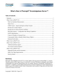
general reference for quasi‐random sequences and methods). Figure 1 shows the relatively high 

discrepancy of a uniform random distribution of 2000 points on the unit square, vs. the much lower 

discrepancy of a 2000 point Sobol sequence of the type used in QRPEM. 

1 

2000 2-dimensional Uniformly Distributed Random Points 

0.9 

0.8 

0.7 

0.6 

0.5 

0.4 

0.3 

0.2 

0.1 

0 

0 0.1 0.2 0.3 0.4 0.5 0.6 0.7 0.8 0.9 1 

1 

2000 2-dimensional Uniformly Distributed Quasi-random Points 

0.9 

0.8 

0.7 

0.6 

0.5 

0.4 

0.3 

0.2 

0.1 

0 

0 0.1 0.2 0.3 0.4 0.5 0.6 0.7 0.8 0.9 1 

Figure 1. Relatively high discrepancy sequence of 2000 uniformly distributed random points (top) vs. 

much lower discrepancy sequence of 2000 uniformly distributed Sobol quasi‐random points (bottom). 

Note the discrepancy is the area of the largest rectangular unpopulated white space that can be found 

within the bounding square. 


The basic concept of a low discrepancy sequence is relatively modern, having originated in the 1960s 

from a variety of contributors. It was later generalized by Niederreiter to (t,m,s) nets (here ‘net ‘ is 

used in an similar but more general sense as ‘grid’) . Practical low discrepancy sequences (some 

common types are Faure, Halton, Niederreiter, Hammersley, and Sobol sequences) first started to 

appear in the late 1960’s. Very fast implementations comparable in speed to the more usual 

pseudorandom number generators are now available for several important cases. Initial applications 

were primarily to numerical integration, particularly in physics and computational finance. Later the 

technique was extended as a potentially more efficient alternative to some, but not all, types of Monte 

Carlo simulation (for example, there are notorious difficulties to applying low discrepancy sequences to 

Markov Chain Monte Carlo based methods such as SAEM, although to some recent progress has been 

made in this area with the introduction of the idea of ‘scrambling’ [6] by Owen and others.) 

The Sobol sequence used in QRPEM is widely regard as being particularly effective for numerical 

integration problems in low dimensional spaces d

TEST 1 – A difficult sparse and highly nonlinear EMAX model. 

Summary of results: QRPEM and NMIMP were compared on a difficult sparse, highly nonlinear PD 

model adapted from a recent set of models used in Mats Karlsson’s lab at Uppsala to compare NM 

SAEM and MONOLIX SAEM to traditional approximate likelihood models. At identical sample sizes of 

500, QRPEM gave excellent results for all parameters in 150 seconds, while NMIMP in 323 seconds gave 

good results on fixed effects but relatively poor estimates for the random effects matrix Omega. The 

sample size for NM IMPEM was then gradually increased to see if the Omega estimates could be 

improved. Indeed, at a sample size of N=200,000, the NMIM Omega results converged almost exactly 

to the QRPEM N=500 Omega results. QR theory in fact predicts convergence at roughly this size, i.e. a 

QR sample size of 500 should be approximately as accurate as a MC sample size of 500 2 = 250000 on 

smooth, low dimensional integrands. NMIMP took 50.2 hours vs. 2.5 minutes for QRPEM to reach the 

same high quality estimate. 

It is important to note that this three order of magnitude time difference is not representative of 

relative timings that should be expected when QRPEM and NMIMP are run in ‘normal’ operating mode. 

Under usual circumstances, both would probably be run with a few hundred samples. In these 

circumstances, QRPEM has proved to be faster by typical factors of 1.5 to 4 than NMIMP run in default 

mode. These relative timings may change as more features are added to QRPEM, or if NMIMP is run in 

some non‐default mode that happens to improve performance on a given model. But we believe the 

real significance is the greatly improved accuracy, precision, and repeatability at equivalent sample sizes 

that QRPEM offers. EM methods like QRPEM, SAEM and MCPEM are often described as ‘exact’ 

likelihood methods as opposed to the approximate likelihood methods like FO and FOCE. This is not 

exactly true. FO and FOCE are indeed approximate likelihood methods, and they produce a certain 

inherent level of accuracy for any given model and data set– there’s nothing the user can do to improve 

it. But SAEM, MCPEM and QRPEM are more correctly described as “likelihood as exact as you want to 

make it” methods. The accuracy of the likelihood depends on the number of samples N in the case of 

QRPEM, and on the number of iterations in the case of SAEM, and the accuracy can be made as high as 

desired if the user is willing to pay for it with computer time. The real advantage of QRPEM is that it 

achieves high accuracy at sample sizes that are computationally reasonable, as opposed to NMIMP 

which often has to be run at very high samples sizes. At a sample size of 300 (the NMIMP default) 

QRPEM obtains results that are often within a few 0.1’s of the true ML ELS OBJ value (see results in 

other test cases below). At this same size, MCPEM and SAEM methods get results with ten times more 

error, so they are within a few 1’s of the ML ELS OBJ value. For some purposes, the MCPEM and SAEM 

results are probably good enough – for example, it is unlikely that the moderate precision MCPEM result 

would lead to a different conclusion in a visual predictive check than the high precision QRPEM result. 

But for other purposes, for example covariate model analysis, the additional precision is important. The 

critical value for determining whether addition of a covariate is statistically significant is an 

improvement of around 3.5 ELS OBJ units. If the method precision is near this level, covariate analyses 

become very problematic. But precision at the QRPEM level is more than adequate for this purpose. 


Details 

At the recent 2011 ACoP conference (and also at the 2010 PAGE conference), Elodie Plan et al [4] 

presented a series of EMAX PD models 

E = E0 + Emax*Dose /(Dose + ED50 

with simulated data in order to compare the performance of NM SAEM and Monolix SAEM to the 

traditional approximate likelihood models (NM IMPEM was not included in the comparison). Here is a 

Hill coefficient that governs the degree of nonlinearity (higher is more nonlinear). 

On several of the test cases SAEM (both Monolix and NM7) gave relatively poor estimates. Perhaps the 

most difficult single case was the sparsest (2 observations per subjects) and most nonlinear (Hill 

coefficient =3). We selected this as a test case for QRPEM and simulated sparse data sets with 1000 

subjects, 2 observations per subject, proportional error model, with the same true parameter values as 

used in the Plan model (our model was different only in the number of subjects, 1000 vs. 100, and the 

fact that we used a fixed value of rather than treating it as a fixed effect to be estimated. 

When run in PHX QRPEM with a sample size of 500, excellent results were obtained for all parameters, 

namely the fixed effects THETA, the random effect parameters OMEGA, and the residual error standard 

deviation. The corresponding NM7 IMPEM results with a sample size of 500 were reasonably good for 

fixed effects but only fair for the random effect Omega parameters, and in particular relatively poor for 

the Omega(EMAX,ED50) parameter. 

True Omega values from simulation are 

E0 EMAX ED50 

0.0900 

0.000 0.490 

0.000 0.245 0.490 

Omega Estimates from QRPEM and NMIMP with N=500 are 

QRPEM N=500 (150 sec) 

NMIMP N=500 (323 sec) 

E0 EMAX ED50 E0 EMA ED50 

0.0939 0.0932 

‐0.00735 0.536 ‐0.0260 0.464 

‐0.00775 0.261 0.472 ‐0.0227 0.137 0 .365 

Note the Omega estimates for QRPEM with a sample size of 500 are considerably different and better 

than the NMIMP estimate with the same sample size, particularly in the omega(EMAX,ED50) element , 

0.261 vs 0.137, and the Omega(ED50,ED50) estimate, 0.472 vs. 0.365. The true values used to simulate 

the data were 0.245 and 0.490, respectively. 


When the sample size for NM IMP is increased to 200,000, the Omega matrix estimate is remarkably 

close to that obtained by QPREP with a sample size of 500: 

NMIMP N=200000 (50.2 hours) 

E0 EMAX ED50 

0.0939 

‐0.00987 0.534 

‐0.0102 0.257 0.471 

As can be seen from the table below, the NM IMP cov(EMAX,ED50) and ELS OBJ value estimates steadily 

improve toward the PHX QRPEM estimate and ELS OBJ value as the sample size increases to very high 

values, so the result for the 200,000 sample size is not a fluke and a sample this large really is required 

to match the QRPEM results. 

NM cov(EMAX,ED50) and ELS OBJ estimates 

N cov(EMAX,ED50) ELS OBJ 

500 0.137 7359.276 

1000 0.158 7351.957 

3000 0.193 7353.849 

10000 0.219 7347.394 

250000 0.225 7343.776 

500000 0.237 7337.368 

2000000 0.257 7340.930 

The QRPEM cov(EMAX,ED50) and ELS OBJ value at ISAMPLE=500 are 0.261 and 7340.241, respectively. 

The 'true value' of cov(EMAX,ED50) used to simulate the data is 0.245. 


TEST 2 – A moderately difficult sparse test model from the 2005 Lyon INSERM Blind Inter‐method 

comparison exercise (see [3] for details of this exercise and the results) 

The original 2005 test model was a 1‐compartment first order oral absorption model with linear first 

order elimination (the usual V, Ke, Ka parameterization was changed to V, Ke, Ka‐Ke to avoid the flipflop 

identifiability problem associated with this model). The original exercise involved 100 sets of 

simulated data with 100 subjects each, approximately 3 observations per subject. All data sets were 

simulated with the same parameter values. For the QRPEM/NMIMP comparison here all data sets were 

merged into a single large set with 10000 subjects and 30000 observations. 

Summary of results: QRPEM was much faster than NMIMP (3208 sec vs. 17502 sec, 210 iterations vs. 

397 iterations with both run with N=300 samples. The QRPEM method ELS OBJ was far better ‐ lower by 

about 55 points (7721.070 vs. 7776.479. Both methods gave parameters in excellent agreement with the 

true values used in the original simulations, except for NMIMP on Omega(Ka‐Ke,Ka‐Ke). This was 

estimated at 0.0220 by QRPEM and 0.0395 by NM IMP vs. a “True” value of 0.0225. The NMIMP 76% 

overestimate is generally consistent with the results found in the original 2005 exercise. All 10 methods 

evaluated at that time had difficulties with overestimating this value, with the best results being 

obtained by SAEM at an average of about a 50% overestimate averaged over the 100 individual data 

sets. The result obtained here by QRPEM (a 2.2 % underestimate) is by far the best result obtained by 

any method. 

Details: 

The Model was a simple one compartment oral first order linear absorption 

Conc =(( Dose*Ka)/V*(Ka‐Ke))*exp(‐Ke*t – exp(‐Ka*t)*exp(eps) 

where eps is a normally distributed random residual error. 

The parameterization was designed to avoid the possibility of flip‐flop associated with this model: 

V=tvV*exp(etaV) 

Ke=tvKe*exp(etaKe) 

Ka=Ke+(tvKa‐Ke)*exp(etaKa‐Ke) 

100 data sets with 100 subjects each with approximately 3 observations per subject were generated by 

simulation, so ‘TRUE” parameter values were known (to the organizers but not the participants). 

Detailed results of the performance of 10 different methods, including SAEM (the precursor to 

MONOLIX), PEM (the precursor to QRPEM), and MCPEM (the precursor to NONMEM IMPEM). Details of 

the original exercise results are given in [3] . Basically, the EM methods in the original exercise all did 

well estimating all the parameters except Omega(Ka‐Ke,Ka‐Ke), with relatively little bias and reasonable 


oot mean square errors. All 10 methods severely overestimated Omega(Ka‐Ke,Ka‐Ke), with SAEM 

being the least biased for this parameter at an average overestimate of 50%. 

Here we concatenated all 100 data sets into a single large data set with 10000 subjects and 

approximately 30000 observations and ran with 300 samples per subject in both QRPEM and NMIMP. 

The detailed estimates of primary interest are 

True QRPEM NMIMP 

tvV 27.2 27.4 27.4 

tvKe 0.232 0.231 0.235 

tvKa‐Ke 0.304 0.311 0.307 

stddeveps 0.250 0.254 0.253 

Omega(V,V) 0.218 0.213 0.214 

Omega(Ke,Ke) 0.655 0.654 0.666 

Omega(Ka‐Ke,Ka‐Ke) 0.0225 0.0220 0.0392 

ELSOBJ 7721.070 7776.479 

RUNTIME 3208 SEC 17502 SEC 

ITERATIONS 210 397 

Note in particular QRPEM achieves a far better estimate of Omega(Ka‐Ke,Ka‐Ke), as well as a much 

better (lower) ELS OBJ value. 


TEST 3: Repeatability and ELS OBJ accuracy test on a relatively easy IV bolus model 

Summary of results: The simplest of the MONOLIX test models accompanying the MONOLXI 2.0 release 

is a rich data single dose 1‐compartment IV bolus model. This was run from a variety of starts with 

QRPEM and NMIMP. Also, very high precision maximum likelihood estimates were obtained with the 

adaptive Gaussian quadrature (AQG) method in Phoenix NLME. All runs gave good estimates in the 

sense that the parameter estimates were in good agreement with the known simulated parameter 

values. However, the QRPEM results were much more repeatable, reproducing each other and the 

correct ML estimate value with 0.1 ELS OBJ units on each run. The NMIMP results were much more 

variable, with results changing by as much as 1.5 EL OBJ units for run to run and typically agreeing with 

the true ML value only within 1.0 units. This repeatability and accuracy is an important consideration 

when performing covariate searches, where imprecision in the ELS OBJ value of the magnitude observed 

in the NMPEM runs may lead to incorrect conclusions regarding the significance of a covariate. 

Details 

AGQ 25 Points ELSOBJ = ‐4041.788 

AGQ 100 Points ELSOBJ= ‐4041.790 

AGQ 400 Points ELSOBJ=‐4041.790 

Further increases in the resolution of the AGQ grid resulted in no changes to either ELSOBJ or parameter 

estimates. 

QRPEM N=300 ELSOBJ=‐4041.749 

QRPEM N=300 start 2 ELSOBJ= ‐4041.749 

QRPEM N=300 start 3 ELSOBJ= ‐4041.749 




Note at three different starts with initial values of random effects changed by as much as 50%, QRPEM 

gave essentially identical results. 

Parameter estimates of the maximum resolution versions of AGQ and QRPEM were identical to at least 

4 significant figures, and the ELSOBJ values were identical to 0.001. We may reasonably conclude that 

both have reached essentially the exact ML estimate. Note that at the ‘typical’ sample size of N=300, 

QRPEM estimates were nearly identical (within 1%) to the ML estimates and the ELSOBJ values were 

within 0.24 units of the true ML values. From a statistical point of view, a 0.24 unit discrepancy is trivial. 

NMIMP N=300 ELSOBJ=‐4040.891 

NMIMP N=300 start2 ELSOBJ= ‐4041.368 

NMIMP N=300 start3 ELSOBJ= ‐4042.353 

Note the much higher variability in NM IMP ELSOBJ values, with a range of 1.5 ELSOBJ points vs. a range 

of 0.000 points over 3 starts for QR PEM. At high precision (N=90000), the NM IMP value was obtained 

as ELSOBJ=‐4040.740, quite close to the ELSOBJ= ‐4040.749 value for QRPEM=300. 


TEST 4 : One compartment single dose models from the 2007 MONOLIX test set 

Background : The MONOLIX 2.0 release in 2007 was accompanied by 150 test cases spread over 24 

basic types of 1‐ and 2‐compartment models, with approximately 6 variations in dosing patterns and 

model parameterizations for each basic model. Here we compared QRPEM, NMIMP, and NMSAEM on 

the 12 base one compartment single dose models with a Ke‐V type of parameterization. The models 

consisted of 6 linear elimination models and 6 nonlinear Michaelis‐Menten elimination models. Despite 

the relative richness of the data, many of these models proved to be quite difficult for NM FOCE, which 

failed to converge on a majority of them. As reported in [5], MONOLIX SAEM succeeded on all models 

in obtaining good estimates in general agreement with known parameter values used to simulate the 

data sets. 

Summary of Results: 

Odd numbered models have linear elimination, even numbered Michaelis‐Menten nonlinear 

elimination. See the Exprimo report in [5] for details of the models and true parameter values. 

Both NMIMP and QRPEM were run at the NMIMP default sampling level of N=300 samples/subject and 

a max iteration count of 2000. NM IMP was run with a convergence criterion CTYPE=3, while NM SAEM 

was run with a maximum of 1000 iterations and CTYPE=1. In all cases NMIMP and QRPEM converged 

well before the maximum iteration limit, while SAEM required the full 1000 iterations. 

NMIMP and QRPEM succeeded on all models, getting parameter estimates in good agreement with 

known parameter simulation values. SAEM succeeded on all but one model, but was judged to have 

failed to get an acceptably good result on that model. Repeated starts from other initial conditions also 

did not succeed, and revealed a large variability for SAEM on this model. 

QRPEM often was significantly faster (typically 1.5X to 3X) than NM IMP for the more complex models), 

and got much closer to the true ML ELS OBJ values as evaluated by the techniques discussed in Test 3. 

NMIMP was faster than NMSAEM by about typical factors of 1.5X to 2X. 

Details ‐ 

Values listed are the ELS OBJ values for each run, as well as the timings. The notation ‘sd’ refers to 

‘single dose’. We plan to add comparisons to other dosage regimens and parameterizations in the near 

future. 

mlx101 sd 

QRPEM ‐4041.749 14 sec 

NMIMP ‐4040.891 20 sec 

NMSAEM ‐4041.471 69 sec 

True ML ELS OBJ value from high precision AGQ : 4041.790 


mlx102 sd 


NMIMP ‐4090.424 165 sec 

NMSAEM ‐4089.632 225 sec 

mlx103 sd 


NMIMP ‐4034.644 20 sec 

NMSAEM ‐4035.201 74 sec 

mlx104 sd 


NMIMP ‐4186.020 176 sec 

NMSAEM ‐4185.848 261 sec 

mlx105 sd 


NMIMP ‐3829.094 23 sec 

NMSAEM ‐3828.736 90 sec 

mlx106 sd 


NMIMP ‐3875.227 221 sec 

NMSAEM ‐3873.968 290 sec 

mlx107 sd 


NMIMP ‐3885.309 24 sec 

NMSAEM ‐3885.061 91 sec 

mlx108 sd 


NMIMP ‐4079.661 567 sec 

NMSAEM ‐4078.293 1051 sec 

mlx109 sd 


NMIMP ‐3230.105 29.5 sec 

NMSAEM ‐3231.311 120 sec 


mlx110 sd 


NMIMP ‐3397.186 133 sec 

NMSAEM ‐3395.371 232 sec 

mlx111 sd (this proved to be a difficult model for SAEM – note the excellent repeatability of the QRPEM 

results relative to NMIMP and NMSAEM) 


QRPEM ‐3511.459 32 sec (alternate start) 

NMIMP ‐3510.741 29 sec 

NMIMP ‐3508.197 50 sec (alternate start) 

NMSAEM ‐3458.423 118 sec , anomalous ELS OBJ value, poor omega 

NMSAEM ‐3484.962 116 (alternate start, still poor Omega estimates) 

mlx112 sd –( as in mlx111 sd, QRPEM is much more repeatable from different starts than NMIMP and 

NMSAEM) 


QRPEM ‐3434.779 301 sec (alternate start) 

NMIMP ‐3434.974 709 sec 

NMIMP ‐3432.923 680 sec (alternate start) 

NMSAEM ‐3431.192 861 sec 

NMSAEM ‐3430.728 842 sec (alternate start) 


TEST 5: Two‐compartment models from the 2007 MONOLIX test set. 

The 12 single dose base case 2‐compartment analogues to the 1‐compartment models discussed in Test 

4 were analyzed with QRPEM and NMPEM. As in the one compartment case, odd‐numbered models 

correspond to linear elimination cases, while even numbered models are considerably more difficult and 

time consuming nonlinear Michaelis‐Menten models. Like the 1‐compartment case, NM FOCE failed to 

converge on most of these models. For each odd numbered model, two data sets were run ‐ a smaller, 

but still rich, single dose data set ‘sd’ and a considerably larger (about 3X as many observations) multiple 

dose data set ‘all’. For the even numbered nonlinear models, currently only sd results are available. 

Summary of Results 

Both QRPEM and NMPEM succeeded on all models, producing good parameter estimates in general 

agreement with the known values used to simulate the data. QRPEM was usually much faster (2X to 5X), 

and also on selected cases where high precision AGQ could be run, far more accurate in ELS OBJ value, 

generally getting the true value within 0.2 ELS OBJ units, as opposed to about 2.0 for NM IMP {data for 

this observation not yet shown) 

Details 

Method/Model Dataset Time ELSOBJ ITERS 

QRPEM201 sd 97 sec 20296.006 80 

NMIMP201 sd 245 sec 20296.391 113 

QRPEM201 all 245 sec 65933.468 60 

NMIMP201 all 223 sec 65932.981 39 

QRPEM202 sd 286 sec ‐4221.047 130 

NMIMP202 sd 1008 sec ‐4220.901 201 


NMIMP203 sd 90 sec 19834.882 41 


NMIMP203 all 122 sec 65133.733 20 


NMIMP204 sd 809 sec ‐4151.040 154 


NMIMP205 sd 222 sec ‐ ‐3801.406 86 

QRPEM205 all 152 sec ‐13696.353 60 


NMIMP205 all 509 sec ‐13696.055 91 


NMIMP206 sd 652 sec ‐4089.790 117 


NMIMP207 sd 213 sec 19554.815 82 


NMIMP207 all 553 sec 64282.751 83 


NMIMP208 sd 902 sec ‐3994.868 86 


NMIMP209 sd 180 Sec ‐3356.903 39 


NMIMP209 all 378 sec ‐13220.921 28 




NMIMP211 sd 557 sec ‐3570.122 179 


NMIMP211 all 1496 sec ‐13488.557 179 


NMIMP 212 sd 1129 sec ‐3692.731 109 


References 

[1] A. Schumitzky. Nonparametric EM Algorithms for Estimating Prior Distributions. App. Math. and 

Computation 45: 143‐158, 1991. 

[2] H. Niederreiter. Random Number Generation and Quasi‐Monte Carlos Methods. SIAM .1992. 

[3] P. Girard and F. Mentre’. A Comparison of Estimation methods in Nonlinear Mixed Effects Models 

Using a Blind Analysis. PAGE 2005. Pamplona, Spain. 

http://www.pagemeeting.org/page/page2005/PAGE2005O08.pdf 

[4] E. Plan, A. Maloney, F. Mentre’, M. Karlsson and J. Bertrand. Performance Comparison of Various 

Maximum Likelihood Nonlinear Mixed‐effects Estimation Methods for Pharmacodynamic Models, 

American Conference on Pharmacometrics. San Diego. April, 2011. http://www.goacop.org/2011/posters 

Also available in an earlier PAGE 2010 version at 

http://www.page‐meeting.org/pdf_assets/4694‐Elodie_Plan_PAGE_Poster.pdf 

[5] C. Laveille, M. Lavielle, K. Chatel, P. Jacqmin . Evaluation of the PK and PK‐PD libraries of MONOLIX: A 

comparison with NONMEM, PAGE 2008; also P.Jacmin, C. Laveille, M. Lavielle, Software Evaluation : 

Simulation of PK Data Sets for Evaluation of the Monolix PK Library, June 6, 2007, Exprimo report. 

[6] A. Owen. Scrambling Sobol and Niederreiter‐Xing points. J. of Complexity 1998. 14:466‐89.

QRPEM – A New Standard of Accuracy, Precision, and ... - Pharsight

Create successful ePaper yourself

Delete template?

Save as template?