A strategy for anisotropic P-wave prestack imaging - PGS

1
A strategy for anisotropic P-wave prestack
imaging
RUBEN D. MARTINEZ AND SHENG LEE
PGS Geophysical, 10550 Richmond Ave., Houston, Texas 77042
Summary
The prestack depth imaging process has been and is continuously evolving with the goal of
accurately position the seismic events in space. To achieve this goal, the prestack imaging
process should account for anisotropy. If the presence of anisotropy is important, then
ignoring it will have a significant impact in the final imaging accuracy. In this paper, we
restrict our discussion to vertical transverse isotropy (VTI) or polar anisotropy.
We propose a strategy that combines anisotropic prestack time and depth imaging. The
strategy consists of a prestack time migration for V(z) and VTI media loop from which the
effective anisotropic (Vnmo and η eff ) parameters are estimated as a function of two-way time.
The strategy continues with the conversion of the effective anisotropic parameters to interval
parameters as functions of depth. Then, the depth imaging loop is executed, here the interval
anisotropic parameters are iteratively refined until the final image is obtained.
The strategy proposed here provides stability to the anisotropic prestack imaging process.
This stability comes from the fact that the anisotropic parameters are first estimated using a
time migration which in turn become the initial parameters for the depth imaging steps.
Introduction
Several methodologies to perform anisotropic prestack imaging have appeared in the
literature. The key for a successful anisotropic imaging is the estimation of the anisotropic
parameters. Some approaches rely on information based on the geologic knowledge of the
area from which appropriate values for the anisotropic parameter, η, are assumed. In other
cases, a simple constant value for η is assumed for the area and the output quality is judged
based on the observed ‘image quality’. Adjustments to the velocities and η are typically
achieved iteratively. But a systematic approach is desired to properly constrain the parameter
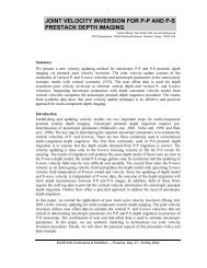
estimation and obtain accurate subsurface images. Figure 1 shows a flow chart which
describes the main steps of the strategy proposed in this contribution.
Anisotropic time imaging.
The first step in our strategy is to perform prestack time migration for V(z) and VTI media
(see Fig.1). This migration approach accounts for the ray bending caused by the vertical
velocity variation with depth and VTI. At least two migration iterations are required to
EAGE 64th Conference & Exhibition — Florence, Italy, 27 - 30 May 2002

2
Amplitude Preserving
Kirchhoff Pre-stack
Time Migration
for V(z) and VTI
Anisotropic Ray
Tracing for P
Waves
• NMO Velocity model vs
time
• η eff model vs time
•Interval Velocity model vs depth
•Interval η model vs depth
•Vertical velocity model vs depth
Controlled
Amplitude
Kirchhoff Prestack
•Sonic logs
•Check shots
•VSP
• Adjust Velocity model in depth
• Adjust Interval η model in depth
Fig.1 Main steps for the proposed anisotropic prestack imaging strategy.
estimate the effective parameters; NMO velocities and effective η. The criteria to decide the
best estimation is when the best focusing (gathers are flat in time) is achieved.
The final results of this step are: an image that is superior to that obtained using a straight ray
prestack time migration and the effective velocities (NMO) and η estimated during the
process. The accuracy of the NMO velocities should be very useful to estimate interval
velocities to be used in the initial iteration of prestack depth migration. Figure 2 shows an
example of a NMO velocity field and the corresponding effective η estimated in this step
using field seismic data.

3
(a)
(b)
Fig.2 (a) Interval velocity field (meters per second in the legend) versus two-way time derived
from the effective time migration velocities; (b) effective η parameter (effective η x 1000 in
the legend) versus two-way time. Both the interval velocities and effective η were smoothed
along layers.
Anisotropic parameters for depth imaging
While prestack time migration for V(z) and VTI media requires two effective parameters
(Vnmo and η eff ), prestack depth migration requires three. These parameters are: interval
velocities (estimated from multichannel seismic data)(V i ), interval vertical velocity (Vo i ) and
the interval anisotropic parameter (η i ). In our strategy (see Fig.1), we propose to compute V i
and η i versus depth from the effective parameters Vnmo and η eff versus two-way time using
the familiar Dix equation for V i and a Dix-type formulation for η i . The parameter Vo i has to
be estimated with help from borehole data, i.e. sonic logs, check shots or zero offset VSP’s.
Anisotropic Depth imaging
Once the interval parameters are calculated from the prestack time migration results, the first
iteration of depth migration is performed. The three interval parameters are used to build
gridded volumes to perform anisotropic ray tracing to generate the traveltimes required for
Kirchhoff depth migration (see Fig.1). The interval anisotropic parameters are adjusted at
every depth migration iteration until the ‘best’ focusing (gathers are flat in depth).
To illustrate the difference between isotropic and anisotropic depth imaging, Figure 3 shows
the results obtained after depth migration. A slight image improvement in the salt flank is
observed in the anisotropic depth imaging result (2 kms)(Fig.3(b)). But more importantly, the
deep seismic horizons apperar at different depths. The isotropic depth imaging produces
deeper horizons than those obtained when VTI is accounted for during depth migration. This
EAGE 64th Conference & Exhibition — Florence, Italy, 27 - 30 May 2002

is particularly clear for the strong event at 4 kms. (black arrows). This depth differences are
mainly driven by the velocities V i and Vo i and are related to the anisotropic parameter δ.
4
(a)
(b)
Fig.3 Results obtained with isotropic (a) and anisotropic (b) depth imaging.
Conclusions.
The proposed strategy provides a stable means for anisotropic prestack imaging and
anisotropic parameter estimation. First, the effective parameters are estimated through
prestack time migration (Vnmo, η eff ) and the process continues with the refinement of the
parameters (V i , Vo i , and η i ) through anisotropic depth migration. The estimated velocities are
accurate after time migration due to the ray bending allowed in the algorithm to account for
V(z) and VTI. The depth imaging loop benefit from this velocity accuracy by assuring a
reliable initial model and therefore reducing the number of iterations necessary to achieve the
final result. Another important point to remark is that isotropic prestack imaging should
always be accomplished prior to the anisotropic equivalent for best results.
Acknowledgements
We would like to thank our colleagues Min Lou and Shelton Ma from PGS Research and DPS
respectively for providing the processing software for the anisotropic parameter estimation
and anisotropic ray tracing stages of the strategy.