Anisotropic prestack depth migration improves the well-ties at ... - PGS
Anisotropic prestack depth migration improves the well-ties at ... - PGS
Anisotropic prestack depth migration improves the well-ties at ... - PGS

Create successful ePaper yourself
Turn your PDF publications into a flip-book with our unique Google optimized e-Paper software.
<strong>Anisotropic</strong> <strong>prestack</strong> <strong>depth</strong> <strong>migr<strong>at</strong>ion</strong> <strong>improves</strong> <strong>the</strong> <strong>well</strong>-<strong>ties</strong> <strong>at</strong> <strong>the</strong> Ewing Bank Oil Field, Gulf<br />
of Mexico<br />
Dario Cegani, ENI E&P, Eduardo Berendson, ENI Petroleum, Clive Hurst, ENI Petroleum, Helen Delome*,<br />
<strong>PGS</strong> Geophysical, USA and Rubén D. Martínez, <strong>PGS</strong> Geophysical, USA<br />
Summary<br />
We successfully applied anisotropic Kirchhoff <strong>prestack</strong><br />
<strong>depth</strong> <strong>migr<strong>at</strong>ion</strong> (AKPreDM) to a 3D d<strong>at</strong>a set from <strong>the</strong><br />
Ewing Bank Oil Field, Gulf of Mexico to accur<strong>at</strong>ely map<br />
<strong>the</strong> target sands in <strong>depth</strong>. Initially, we used isotropic<br />
Kirchhoff <strong>prestack</strong> <strong>depth</strong> <strong>migr<strong>at</strong>ion</strong> (IKPreDM) to perform<br />
<strong>the</strong> mapping of <strong>the</strong> reservoir sands. However, <strong>the</strong> <strong>depth</strong>s<br />
estim<strong>at</strong>ed using <strong>the</strong> seismic d<strong>at</strong>a and those detected <strong>at</strong> <strong>the</strong><br />
<strong>well</strong>s for <strong>the</strong> target sands showed excessive miss-<strong>ties</strong><br />
(approxim<strong>at</strong>ely 1100 feet). The results obtained after <strong>the</strong><br />
applic<strong>at</strong>ion of AKPreDM showed th<strong>at</strong> <strong>the</strong> miss-<strong>ties</strong> were<br />
gre<strong>at</strong>ly reduced within a few tens of feet, <strong>the</strong>refore<br />
providing a better tie with <strong>the</strong> <strong>well</strong> tops. In this paper, we<br />
present <strong>the</strong> methodology employed in this case study,<br />
which includes <strong>the</strong> anisotropic parameter estim<strong>at</strong>ion. We<br />
also discuss <strong>the</strong> <strong>well</strong> tie results obtained after <strong>the</strong><br />
applic<strong>at</strong>ion of AKPreDM and IKPreDM. We conclude th<strong>at</strong><br />
<strong>the</strong> effect of anisotropy (vertical transverse isotropy, VTI)<br />
should be taken into account to obtain seismic <strong>depth</strong><br />
estim<strong>at</strong>es th<strong>at</strong> better tie <strong>the</strong> <strong>well</strong> <strong>depth</strong>s accur<strong>at</strong>ely.<br />
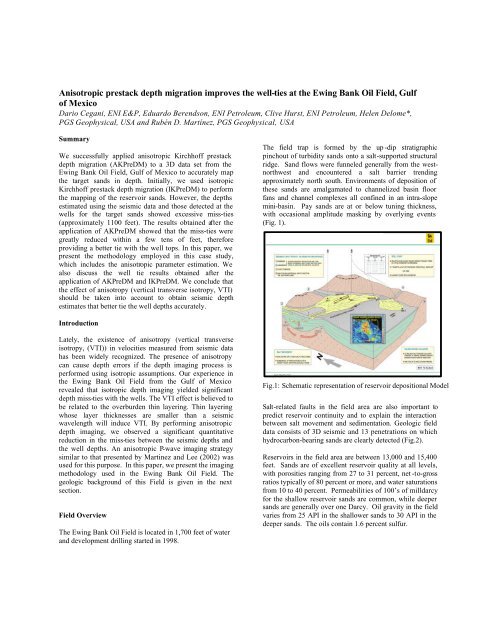
The field trap is formed by <strong>the</strong> up -dip str<strong>at</strong>igraphic<br />
pinchout of turbidity sands onto a salt-supported structural<br />
ridge. Sand flows were funneled generally from <strong>the</strong> westnorthwest<br />
and encountered a salt barrier trending<br />
approxim<strong>at</strong>ely north south. Environments of deposition of<br />
<strong>the</strong>se sands are amalgam<strong>at</strong>ed to channelized basin floor<br />
fans and channel complexes all confined in an intra-slope<br />
mini-basin. Pay sands are <strong>at</strong> or below tuning thickness,<br />
with occasional amplitude masking by overlying events<br />
(Fig. 1).<br />
Introduction<br />
L<strong>at</strong>ely, <strong>the</strong> existence of anisotropy (vertical transverse<br />
isotropy, (VTI)) in veloci<strong>ties</strong> measured from seismic d<strong>at</strong>a<br />
has been widely recognized. The presence of anisotropy<br />
can cause <strong>depth</strong> errors if <strong>the</strong> <strong>depth</strong> imaging process is<br />
performed using isotropic assumptions. Our experience in<br />
<strong>the</strong> Ewing Bank Oil Field from <strong>the</strong> Gulf of Mexico<br />
revealed th<strong>at</strong> isotropic <strong>depth</strong> imaging yielded significant<br />
<strong>depth</strong> miss-<strong>ties</strong> with <strong>the</strong> <strong>well</strong>s. The VTI effect is believed to<br />
be rel<strong>at</strong>ed to <strong>the</strong> overburden thin layering. Thin layering<br />
whose layer thicknesses are smaller than a seismic<br />
wavelength will induce VTI. By performing anisotropic<br />
<strong>depth</strong> imaging, we observed a significant quantit<strong>at</strong>ive<br />
reduction in <strong>the</strong> miss-<strong>ties</strong> between <strong>the</strong> seismic <strong>depth</strong>s and<br />
<strong>the</strong> <strong>well</strong> <strong>depth</strong>s. An anisotropic P-wave imaging str<strong>at</strong>egy<br />
similar to th<strong>at</strong> presented by Martinez and Lee (2002) was<br />
used for this purpose. In this paper, we present <strong>the</strong> imaging<br />
methodology used in <strong>the</strong> Ewing Bank Oil Field. The<br />
geologic background of this Field is given in <strong>the</strong> next<br />
section.<br />
Field Overview<br />
The Ewing Bank Oil Field is loc<strong>at</strong>ed in 1,700 feet of w<strong>at</strong>er<br />
and development drilling started in 1998.<br />
Fig.1: Schem<strong>at</strong>ic represent<strong>at</strong>ion of reservoir depositional Model<br />
Salt-rel<strong>at</strong>ed faults in <strong>the</strong> field area are also important to<br />
predict reservoir continuity and to explain <strong>the</strong> interaction<br />
between salt movement and sediment<strong>at</strong>ion. Geologic field<br />
d<strong>at</strong>a consists of 3D seismic and 13 penetr<strong>at</strong>ions on which<br />
hydrocarbon-bearing sands are clearly detected (Fig.2).<br />
Reservoirs in <strong>the</strong> field area are between 13,000 and 15,400<br />
feet. Sands are of excellent reservoir quality <strong>at</strong> all levels,<br />
with porosi<strong>ties</strong> ranging from 27 to 31 percent, net -to-gross<br />
r<strong>at</strong>ios typically of 80 percent or more, and w<strong>at</strong>er s<strong>at</strong>ur<strong>at</strong>ions<br />
from 10 to 40 percent. Permeabili<strong>ties</strong> of 100’s of milldarcy<br />
for <strong>the</strong> shallow reservoir sands are common, while deeper<br />
sands are generally over one Darcy. Oil gravity in <strong>the</strong> field<br />
varies from 25 API in <strong>the</strong> shallower sands to 30 API in <strong>the</strong><br />
deeper sands. The oils contain 1.6 percent sulfur.
<strong>Anisotropic</strong> <strong>prestack</strong> <strong>depth</strong> <strong>migr<strong>at</strong>ion</strong> <strong>improves</strong> <strong>the</strong> <strong>well</strong>-<strong>ties</strong> <strong>at</strong> <strong>the</strong> Ewing Bank Oil Field, Gulf of Mexico<br />
simultaneously with <strong>the</strong> η eff (Min et. al., 2002). We<br />
proved th<strong>at</strong> smoothing <strong>the</strong> η eff model provided more<br />
stability. After some testing, <strong>the</strong> final η eff model was<br />
determined by averaging <strong>the</strong> interval η values around <strong>the</strong><br />
#1 <strong>well</strong>. We used only one interval η defined in one layer.<br />
The layer was defined between <strong>the</strong> w<strong>at</strong>er bottom and a<br />
surface above <strong>the</strong> reservoir, and <strong>the</strong> interval η value was set<br />
to 0.012. This surface was interpreted (from <strong>the</strong> isotropic<br />
final stack volume) as <strong>the</strong> bottom of <strong>the</strong> sand/shale<br />
sequence in <strong>the</strong> area (see Figs.3 and 4). We concluded th<strong>at</strong><br />
this layer was <strong>the</strong> main cause of <strong>the</strong> VTI effect.<br />
Fig.2 Salt mini-basins in field area. In blue (dark) is <strong>the</strong><br />
sp<strong>at</strong>ial distribution of a key reservoir in <strong>the</strong> field. Yellow<br />
lines show some of <strong>the</strong> <strong>well</strong>s in <strong>the</strong> field.<br />
η=0.012<br />
Depth imaging in <strong>the</strong> presence of anisotropy<br />
We first performed isotropic <strong>depth</strong> imaging resulting in<br />
common image ga<strong>the</strong>rs (CIGs) th<strong>at</strong> were nearly fl<strong>at</strong> in<br />
<strong>depth</strong>, but <strong>the</strong> seismic <strong>depth</strong>s obtained <strong>at</strong> <strong>the</strong> reservoir<br />
levels were off to those detected <strong>at</strong> <strong>the</strong> <strong>well</strong>s. The miss-tie<br />
estim<strong>at</strong>ed <strong>at</strong> <strong>the</strong> oil field was about 1100 ft. This prompted<br />
us to investig<strong>at</strong>e <strong>the</strong> possibility of having velocity<br />
anisotropy effects in <strong>the</strong> area.<br />
To test <strong>the</strong> hypo<strong>the</strong>sis of having velocity anisotropy, we<br />
used <strong>the</strong> anisotropic P-wave imaging str<strong>at</strong>egy proposed by<br />
Martinez and Lee (2002). The most difficult part in<br />
anisotropic imaging is <strong>the</strong> estim<strong>at</strong>ion of <strong>the</strong> parameters th<strong>at</strong><br />
describe <strong>the</strong> vertical transverse isotropy (VTI). Three<br />
parameters are necessary to define a VTI medium: interval<br />
seismic velocity; interval vertical velocity; and <strong>the</strong> interval<br />
anelliptical parameter η.<br />
Fig.3 The one layer η eff model.<br />
Interval seismic velocity model building: The isotropic<br />
final sediment velocity model was used as <strong>the</strong> initial<br />
seismic velocity model for <strong>the</strong> anisotropic <strong>depth</strong> imaging<br />
process.<br />
h model building: The CIGs were stretched to time and <strong>the</strong><br />
isotropic interval velocity model was converted to RMS<br />
velocity in time to pick <strong>the</strong> effective η. The effective η<br />
functions were converted to interval η in <strong>depth</strong> using <strong>the</strong><br />
Dix type formula given in Alkhalifah, T., 1997, which uses<br />
<strong>the</strong> corresponding velocity model.<br />
Many tests were conducted to cre<strong>at</strong>e a stable η eff model.<br />
The effective RMS veloci<strong>ties</strong> were determined<br />
Fig.4 Depth horizon map for <strong>the</strong> base of <strong>the</strong><br />
sand/shale sequence.
<strong>Anisotropic</strong> <strong>prestack</strong> <strong>depth</strong> <strong>migr<strong>at</strong>ion</strong> <strong>improves</strong> <strong>the</strong> <strong>well</strong>-<strong>ties</strong> <strong>at</strong> <strong>the</strong> Ewing Bank Oil Field, Gulf of Mexico<br />
Interval vertical velocity model building: The vertical<br />
velocity model was computed from <strong>the</strong> interval seismic<br />
velocity model and <strong>the</strong> interval vertical veloci<strong>ties</strong> measured<br />
in <strong>well</strong>s using VSP check shots. We transformed both<br />
veloci<strong>ties</strong> from interval to RMS veloci<strong>ties</strong>. We <strong>the</strong>n used a<br />
linear rel<strong>at</strong>ionship assumption between <strong>the</strong> two veloci<strong>ties</strong>,<br />
i.e., V RMS-vert = A + B*V RMS-seis , where <strong>the</strong> coefficients A<br />
and B are constant. The A and B coefficients were obtained<br />
from <strong>the</strong> cross-plots of <strong>the</strong> RMS seismic veloci<strong>ties</strong> in time<br />
<strong>at</strong> <strong>well</strong> loc<strong>at</strong>ions and <strong>the</strong> RMS vertical (<strong>well</strong>) veloci<strong>ties</strong> in<br />
time computed from <strong>the</strong> VSP check shots. Two of <strong>the</strong><br />
straightest <strong>well</strong>s: #1 and #2 were used for this analysis.<br />
Both <strong>well</strong>s were used to compute A and B <strong>at</strong> <strong>the</strong> two <strong>well</strong><br />
loc<strong>at</strong>ions. For <strong>the</strong> #1 <strong>well</strong>, A=395 and B=0.75 (see Figure<br />
5-a). For <strong>the</strong> #2 <strong>well</strong>, A = 425 and B=0.727 (see Figure 5-<br />
b). An anchor was put <strong>at</strong> <strong>the</strong> loc<strong>at</strong>ion (2138, 6660) for zero<br />
anisotropy effect (A=0, B=1). Volumes of A and B (A(x,y)<br />
and B(x,y)) were computed by triangular interpol<strong>at</strong>ion of<br />
<strong>the</strong> 3 values <strong>at</strong> <strong>the</strong> 3 loc<strong>at</strong>ions. Thus, V RMS-vert in time was<br />
computed and converted to interval velocity<br />
V<strong>well</strong>-rms (m/s)<br />
2500<br />
2000<br />
1500<br />
1000<br />
500<br />
#1 Well<br />
0<br />
-500 0 500 1000 1500 2000 2500<br />
V1-rms (m/s)<br />
in <strong>depth</strong> and minor smoothing was applied. The w<strong>at</strong>er layer<br />
was <strong>the</strong>n re-inserted in <strong>the</strong> vertical interval velocity model.<br />
Having <strong>the</strong> interval seismic velocity, interval η and <strong>the</strong><br />
interval vertical velocity models, <strong>the</strong> next step in<br />
AKPreSDM was to perform anisotropic ray tracing for <strong>the</strong><br />
anisotropic traveltimes calcul<strong>at</strong>ion. The traveltimes were<br />
<strong>the</strong>n used in anisotropic Kirchhoff <strong>prestack</strong> <strong>depth</strong> <strong>migr<strong>at</strong>ion</strong><br />
(AKPreSDM). New CIGs were obtained to perform <strong>the</strong><br />
upd<strong>at</strong>e of <strong>the</strong> anisotropic parameters for <strong>the</strong> next iter<strong>at</strong>ion.<br />
The <strong>depth</strong> sections and ga<strong>the</strong>rs were used for QC and <strong>well</strong>tie<br />
analysis. The <strong>depth</strong> miss-tie was small <strong>at</strong> <strong>the</strong> central and<br />
north of <strong>the</strong> field (+41 to +65 ft <strong>at</strong> <strong>the</strong> #1 <strong>well</strong>, and -49 to –<br />
39ft <strong>at</strong> <strong>the</strong> #2 <strong>well</strong>). Meanwhile in <strong>the</strong> Sou<strong>the</strong>rn part of <strong>the</strong><br />
field, <strong>the</strong> miss-<strong>ties</strong> were larger (about -175ft).<br />
Vrms<br />
Linear (Vrms)<br />
Fig. 5-a Cross-plot of RMS vertical (<strong>well</strong>) veloci<strong>ties</strong><br />
versus RMS seismic veloci<strong>ties</strong>.<br />
V<strong>well</strong>-rms (m/s)<br />
2500<br />
2000<br />
1500<br />
1000<br />
500<br />
# 2 Well<br />
0<br />
-500 0 500 1000 1500 2000 2500<br />
V1-rms (m/s)<br />
Fig. 5-b Cross-plot of RMS vertical (<strong>well</strong>) veloci<strong>ties</strong><br />
versus RMS seismic veloci<strong>ties</strong>.<br />
Based on <strong>the</strong>se results, ano<strong>the</strong>r velocity refinement step<br />
was undertaken with <strong>the</strong> objective to reduce <strong>the</strong> <strong>well</strong> <strong>depth</strong><br />
to seismic <strong>depth</strong> miss-tie.<br />
The upd<strong>at</strong>ed velocity functions were re-gridded and<br />
properly smoo<strong>the</strong>d to gener<strong>at</strong>e a new interval seismic<br />
velocity volume. Cross-plots of <strong>the</strong> new RMS seismic<br />
veloci<strong>ties</strong> versus <strong>the</strong> RMS vertical veloci<strong>ties</strong> <strong>at</strong> <strong>the</strong> two <strong>well</strong><br />
loc<strong>at</strong>ions were re-computed to gener<strong>at</strong>e <strong>the</strong> new linear<br />
rel<strong>at</strong>ionship. For <strong>the</strong> #1 <strong>well</strong>, <strong>the</strong> rel<strong>at</strong>ion was very close to<br />
<strong>the</strong> previous iter<strong>at</strong>ion (A=400 and B=0.75), but for <strong>the</strong> #2<br />
<strong>well</strong> a slight change was needed (A = 415 and B=0.739).<br />
The anchor <strong>at</strong> (2138, 6660) for zero anisotropy was still in<br />
effect (A=0, B=1). New volumes of A and B (A(x,y) and<br />
B(x,y)) were computed by triangular interpol<strong>at</strong>ion of <strong>the</strong><br />
three values <strong>at</strong> <strong>the</strong> three loc<strong>at</strong>ions. A new interval vertical<br />
velocity in <strong>depth</strong> (V vert ) was re-cre<strong>at</strong>ed in <strong>the</strong> same way as<br />
<strong>the</strong> previous iter<strong>at</strong>ion. The interval η model was kept<br />
unchanged.<br />
<strong>Anisotropic</strong> Model Verific<strong>at</strong>ion Tests<br />
To prove <strong>the</strong> accuracy of <strong>the</strong> models, a model verific<strong>at</strong>ion<br />
test was conducted to output PSDM ga<strong>the</strong>rs for 10 inlines<br />
and 3 cross-lines: inlines 1926, 1936, 1938, 1942, 1944,<br />
1946, 1950, 1954, 1964, and 1978, cross-lines 5892, 5896,<br />
and 5900. The ga<strong>the</strong>rs and stacks were used for a <strong>well</strong>-tie<br />
analysis. We found th<strong>at</strong> <strong>the</strong> miss-tie away from <strong>the</strong> #1 <strong>well</strong><br />
(especially in <strong>the</strong> Sou<strong>the</strong>rn part of <strong>the</strong> field) was improved<br />
while <strong>at</strong> this <strong>well</strong> loc<strong>at</strong>ion <strong>the</strong> miss-tie was slightly<br />
increased (~+100ft). The ga<strong>the</strong>rs were acceptably fl<strong>at</strong>. We<br />
performed additional analyses to understand <strong>the</strong> possible<br />
factors th<strong>at</strong> would have affected <strong>the</strong> <strong>depth</strong> <strong>ties</strong> and to<br />
propose solutions for better <strong>depth</strong> <strong>ties</strong> without degrading<br />
<strong>the</strong> image quality. We found th<strong>at</strong> <strong>the</strong> VSP check shot of <strong>the</strong><br />
#2 <strong>well</strong> was not useful because <strong>the</strong>re were measurements<br />
only between 3.9 seconds to 4.5 seconds (below <strong>the</strong><br />
sand/shale sequence). So <strong>the</strong> vertical velocity model was<br />
Vrms<br />
Linear (Vrms)
<strong>Anisotropic</strong> <strong>prestack</strong> <strong>depth</strong> <strong>migr<strong>at</strong>ion</strong> <strong>improves</strong> <strong>the</strong> <strong>well</strong>-<strong>ties</strong> <strong>at</strong> <strong>the</strong> Ewing Bank Oil Field, Gulf of Mexico<br />
re-built by using only <strong>the</strong> linear rel<strong>at</strong>ion from <strong>the</strong> #1 <strong>well</strong>.<br />
This rel<strong>at</strong>ion was re-computed by using <strong>the</strong> measurements<br />
above <strong>the</strong> reservoir (3.8 seconds and <strong>at</strong> earlier times). The<br />
new values of A= 385 and B=0.75 were obtained from a<br />
new cross-plot.<br />
The PSDM ga<strong>the</strong>rs for <strong>the</strong> same 10 inlines were output for<br />
this new vertical velocity model. The stacked sections<br />
showed <strong>the</strong> best <strong>depth</strong> <strong>ties</strong> <strong>at</strong> <strong>the</strong> <strong>well</strong> loc<strong>at</strong>ions. The ga<strong>the</strong>rs<br />
were reasonably fl<strong>at</strong>. Figures 6 and 7 show portions of <strong>the</strong><br />
migr<strong>at</strong>ed stacked sections <strong>at</strong> <strong>the</strong> loc<strong>at</strong>ions of <strong>well</strong>s #1 and<br />
#2 respectively.<br />
Fig. 7 Comparison of isotropic (right) and anisotropic<br />
(left) <strong>depth</strong> imaging results <strong>at</strong> <strong>the</strong> #2 <strong>well</strong> loc<strong>at</strong>ion. The<br />
isotropic PSDM image (right) was shifted 1100 ft to try<br />
to tie <strong>the</strong> <strong>well</strong>.<br />
Fig. 6 Comparison of isotropic (right) and anisotropic<br />
(left) <strong>depth</strong> imaging results <strong>at</strong> <strong>the</strong> #1 <strong>well</strong> loc<strong>at</strong>ion. The<br />
isotropic PSDM image (right) was shifted 1100 ft to try<br />
to tie <strong>the</strong> <strong>well</strong>.<br />
Conclusions<br />
Through this case study, we demonstr<strong>at</strong>ed th<strong>at</strong> velocity<br />
anisotropy significantly impacts <strong>the</strong> seismic <strong>depth</strong>s<br />
estim<strong>at</strong>ed using Kirchhofff <strong>prestack</strong> <strong>depth</strong> <strong>migr<strong>at</strong>ion</strong> in <strong>the</strong><br />
Ewing Oil Field.<br />
When <strong>the</strong> <strong>depth</strong> <strong>migr<strong>at</strong>ion</strong> process is performed with<br />
corrections for <strong>the</strong> VTI effect, <strong>the</strong> miss-<strong>ties</strong> with <strong>the</strong> <strong>well</strong><br />
tops are gre<strong>at</strong>ly reduced. The image quality was, in general,<br />
improved, e.g. see figure 7.<br />
As a result of <strong>the</strong> anisotropy corrections, <strong>the</strong> structural<br />
behavior of <strong>the</strong> reservoir sands changed with respect to th<strong>at</strong><br />
obtained with isotropic <strong>depth</strong> <strong>migr<strong>at</strong>ion</strong>. To valid<strong>at</strong>e <strong>the</strong><br />
structural results from both isotropic and anisotropic <strong>depth</strong><br />
<strong>migr<strong>at</strong>ion</strong>s, dipmeter logs may be used to compare <strong>the</strong> dips<br />
estim<strong>at</strong>ed from <strong>the</strong> seismic d<strong>at</strong>a with those of <strong>the</strong> dipmeter<br />
log.<br />
References<br />
Alkhalifah, T., 1997, Velocity analysis using nonhyperbolic<br />
moveout in transversely isotropic media, Geophysics 62,<br />
1839-1845.<br />
Martinez, R.D. and Lee, S., 2002, A str<strong>at</strong>egy for anisotropic<br />
P-wave <strong>prestack</strong> imaging, 72 nd Ann. Intern<strong>at</strong>. Mtg., Soc.<br />
Expl. Geophys., Expanded Abstracts, 149-152.<br />
Acknowledgments<br />
The authors of this paper would like to thank ENI<br />
Petroleum for granting permission to publish this paper.<br />
We also thank ENI Petroleum for providing <strong>the</strong> oil field<br />
background inform<strong>at</strong>ion and migr<strong>at</strong>ed d<strong>at</strong>a sets to illustr<strong>at</strong>e<br />
this paper.