Calculating Phosphorescence Lifetimes

FLUORESCENCE
APPLICATION NOTE
Calculating Phosphorescence Lifetimes with the
Perkin Elmer Model LS-50B
Phosphorescence lifetimes (sometimes referred to as Timed Resolved Fluorescence, TRF)
can be easily calculated with the Perkin Elmer LS-50B. In the procedure described below,
Microsoft Excel® is recommended for calculation of the log of intensities, and the linear
regression of the log values. The procedure described is valid for FLWinLab Rev. 3.00.
Procedure
1. After the LS-50B and FLWinLab have been started, and communication established, click on
the Configuration option under the Utilities menu. Check the Expert Mode option and click
on OK. Next, click on the LS-50B Status option under the Application menu.
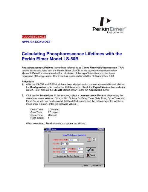
2. Click on the Source icon. In this window, select a Luminescence Mode of phos using the
drop-down arrow selector. Click on OK. Options for Delay Time, Gate Time, Cycle Time, and
Flash Count will now be displayed. All the default values and the entries expected will be in
msec units. To start, enter the following values…
Delay Time: 0.05 msec.
Gate Time: 1.0 msec
Cycle Time: 20 msec
Flash Count: 1
When completed, the window should appear as follows…

Click on Measure and Set Dark Current. Click on OK. The LS-50B Status window may be
left open, or may be minimized.
3. Place sample in holder.
4. Click on the Read option under the Application Menu. Fill in appropriate excitation/emission
wavelengths, and excitation/emission slits for the compound to be measured. Use 5/5 ex/em
slits if correct slit settings are not known. Check the Save on Stop button, and enter a 1
second integration time. Enter an appropriate Destination Filename (i.e., life1.txt). When
completed the Read dialogue should appear similar to the figure below…

Click on the User Info tab and enter the set Delay time (i.e., 0.05) value into the Comments
section. Important: only enter the Delay time value, not other text information, as shown
below.
5. When ready, click on the Green Stoplight button. The sample intensity value will be
displayed. Click on Red Stoplight to stop the read and store the result.
Important: if the intensity is at 999.99 (off-scale), minimize the Read window, and re-open
(maximize) the LS-50B Status window. Click on the source icon and enter a higher value for
the delay time (i.e., 0.1 msec). Re-read sample. If still off-scale, enter a higher delay value
yet, and/or decrease the emission slit. Re-read the sample. If below 999.99 intensity then
continue.
6. Minimize the Read window. Again, maximize the LS-50B Status window. Click on the Source
icon. Enter a Delay value higher than the prior delay value (i.e., 0.1). Click on the Measure
and Set Dark Current button. Click on OK. Maximize the Read window. Again, in the
Comments section, enter the value for the delay time. Click on the Green Stoplight to read
the intensity. Click on the Red Stoplight to end the read. The intensity values should get lower
with increasing delay times for a proper timed resolved experiment.
7. Repeat the above procedure of entering higher and higher delay times, and reading the
intensities under these delay times, recording the delay time numerical value in the
Comments section. Read until the intensity values approach zero. Tailor the experiment to
contain at least six delay time reads. If a misread occurs (i.e., if the proper delay time is not
entered), the resulting file can be edited in Excel.
8. When completed, open the data file in Excel. Note – this file will be stored in the default
FLWinLab data directory C:\FLWINLAB\DATA. A typical file should look similar as below.
The F and G columns contain the intensities and delay times, respectively.
9. The first step in calculating the lifetime is to calculate the natural log of the intensity
values. In the above example, the wells F3 to F9 (column Int.) are to be calculated. Place
cursor in H3 (the column to the right of the Comment column), and type…
=LN (F3)
The natural log of 148.753 (in this example) should be calculated and placed in H3. Copy the
formula in H3 through to H9. The natural log values should now be displayed to the right of
the Comments column as shown in the example below…

10. Next, calculate the linear regression line to the delay time column and log intensity column.
In Excel, this function is LINEST. The result (slope) should be placed below the log data
column in Well H10.
11. The lifetime is the negative reciprocal of the slope. In Well H11 type the following…
= - (1/H10)
12. The lifetime (in msec) will be calculated and placed in H11 as shown in the example
below…In this example for Europium (III) thenoyltrifluoroacetonate (EuTTFA), a lifetime of
0.33 msec was determined.
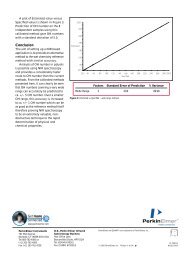
13. If desired, the lifetime graph can be plotted using the Chart tools of Excel, as illustrated
below…
EuTTFA Lifetime
Intensity
6
5
4
3
2
1
0
1 2 3 4 5 6 7
Delay time (ms)