The Focus - Issue 12 - PADT

Contents 

The Focus - Issue 12 

Contents 

A Publication for ANSYS Users 

Feature Articles 

● 

● 

● 

Programming with Tcl/Tk in ANSYS 

Restarting an ANSYS Run 

Testing Elastomers for ANSYS 

On the Web 

● 

● 

ANSYS Releases Variational Design 

Technology 

ANSYS 7.0 New Features 

Resources 

● 

● 

● 

● 

PADT Support: How can we help? 

Upcoming Training at PADT 

About The Focus 

❍ The Focus Library 

❍ Contributor Information 

❍ Subscribe / Unsubscribe 

❍ Legal Disclaimer 

Next in The Focus 

© 2002, by Phoenix Analysis & Design Technologies, Inc. All rights reserved. 

http://www.padtinc.com/epubs/focus/common/contents.asp [11/23/2004 4:47:01 PM]



Programming with Tcl/Tk in 

ANSYS 

by Matt Sutton 


Introduction 

In this article we will explore programming with tcl/tk (pronounced tickle 

tee-kay) in ANSYS. Tcl, an acronym that stands for Tool Command Language, is 

an embedded programming language that was developed by John Ousterhout in 

the late 1980s while he was a professor at Berkeley. Initially, tcl grew out of a 

need for a simple, embeddable command language that Dr. Ousterhout and his 

colleagues could reuse within different integrated circuit design tools that they 

were developing at the time [1]. In a recent article, Dr. Ousterhout outlined the 

requirements he had in mind when he created tcl. 

The notion of embeddability is one of the most unique aspects of Tcl, and it led 

me to the following three overall goals for the language: 

● The language must be extensible: it must be very easy for each application 

http://www.padtinc.com/epubs/focus/2002/0012_1125/article1.htm (1 of 11) [11/23/2004 4:47:52 PM]




● 

● 

to add its own features to the basic features of the language, and the 

application-specific features should appear natural, as if they had been 

designed into the language from the start. 

The language must be very simple and generic, so that it can work easily 

with many different applications and so that it doesn't restrict the features 

that applications can provide. 

Since most of the interesting functionality will come from the application, 

the primary purpose of the language is to integrate or glue together the 

extensions. Thus the language must have good facilities for integration. [1] 

Shortly after developing tcl, Dr. Ousterhouts interests shifted from integrated 

circuit design tools to graphical user interfaces (GUIs). At this time, again in the 

late 1980s, GUIs were still very much in their infancy. Furthermore, the 

manpower needed at that time to develop a usable GUI was rather substantial. 

Driven by a fear that his research team would be under staffed to tackle complex 

GUI development projects, Dr. Ousterhout realized that substantial interactive 

systems could be built out of smaller reusable components, which were then 

programmatically glued together. It was clear to Dr. Ousterhout that the tcl 

language would be ideal as the programmatic glue for such interactive systems, 

if only there existed a set of GUI components from which to build a system. 

Consequently, he begin developing tk in order to fulfill the need for a toolkit of 

reusable GUI components. 

Tcl/tk began to gain popularity throughout the software development community 

primarily via word-of-mouth. Today it is widely used throughout a plethora of 

industries largely because the source code for the tcl interpreter is freely available 

for download from the internet [2]. 

Furthermore, the 5.7 release of ANSYS marked a substantial advancement of tcl 

within ANSYS. Within the 5.7 release, a fully functional tcl interpreter was 

exposed via the ~eui external command. Each subsequent release of ANSYS has 

continued to add functionality based on tcl/tk, culminating in the ANSYS 6.1 

release in which the new GUI is completely implemented with tcl/tk. 

The remainder of this article focuses on programming with tcl/tk in ANSYS. We 

will first briefly look at the tcl language and the tk toolkit in a generic sense. Then 

we will explore ways in which programs written in tcl can be written to interface 

directly with ANSYS. Finally, we will wrap up some loose ends and discuss a few 

of the more advanced aspects of tcl that help mitigate complexity in large 

projects. 





The Tcl/Tk Programming Language 

Tcl is an interpreted command language, and as such, requires an external piece 

of software known as the interpreter, which executes a tcl program stored in a text 

file. Outside of ANSYS, two interpreters are widely used: tclsh and wish. Tclsh 

simply implements the core tcl language, whereas wish extends the tclsh 

interpreter by natively exposing the tk toolkit. Therefore, GUI applications written 

outside of ANSYS should be executed using the wish interpreter. Since wish is a 

superset of tclsh, it can be used exclusively if desired. Inside of ANSYS, the 

equivalent of a wish interpreter is provided by the ~eui external command. Since 

this article focuses on tcl/tk within ANSYS, we will execute all of the example 

programs from within ANSYS via the ~eui command. However, I have often 

found that I am more productive initially if I begin developing a new application 

outside of ANSYS using an off the shelf tcl interpreter [2]. Only after the 

application is functioning correctly do I typically move into ANSYS. 

Lets begin with the prototypical example application used to introduce all 

modern programming languages; the Hello World app. Please follow the steps 

below to create this application. 

1. Launch ANSYS and note the working directory. 

2. Launch you favorite text editor and type in the listing shown in Figure 1. 

Tcl is case sensitive and somewhat non-freeform. Therefore it is imperative 

that you type the program in exactly as it is listed in Figure 1. 

3. Save this file in the current ANSYS working directory with the name 

hello1.tcl 

4. Execute this script in ANSYS using the ANSYS command listed at the 

bottom of Figure 2. 

proc HelloWorld1 {} { 

puts Hello World! 

} 

HelloWorld1 

Figure 1. First "Hello World" application. 

~eui, source [file join [pwd] hello1.tcl] 





Figure 2. Command to execute a tcl script within ANSYS that is located in the 

current working directory. 

Follow these steps and you should see the string Hello World! printed in the 

ANSYS output window. 

As you can see, tcl has a syntax that is very similar to the C programming 

language. It is a structured, procedural language that has a rich set of control 

structures. The first line in our example program declares a procedure named 

HelloWorld1. Procedures in tcl are analogous to functions in C or subroutines 

in FORTRAN. The second line calls a built-in tcl procedure named puts which 

prints a string to the standard output. The third line contains the closing brace for 

the procedure, and the final line simply calls the procedure named HelloWorld1. 

You will notice that there is no main function. In fact, execution in tcl begins with 

the first executable statement, which in this case is the last line. Consequently, 

this program could have simply been written using a single line: puts Hello 

World! 

The fundamental data type in tcl is the string. Consequently, all variables used in 

a tcl program are represented within the tcl interpreter as strings. This provides a 

great deal of flexibility at a small cost in performance. Remember, however, tcl is 

not intended to be a computational workhorse, but rather a glue language, so the 

performance hit for typical glue code should be negligible. The second most 

common data type in tcl is the list. Internally, a list is stored within tcl as a special 

kind of string. A list allows you to effortlessly manipulate a collection of data. 

Before we move to the next example there is one last concept regarding variables 

that needs to be mentioned, that is the concept of scope. Variables within tcl can 

live within one of two scopes: the local or global scope. (Tcl namespaces add an 

additional scope, however, namespaces will not be discussed in this article.) The 

following example demonstrates the concept of local and global variables as well 

as lists and function arguments. 

proc Hello2 {People} { 

global Salutation 

foreach Person $People { 

puts Hello $Person 

} 

set NumberOfPeople [llength $People] 

if { $NumberOfPeople > 1 } { 

puts I said hello to $NumberOfPeople people. 




} else { 

puts I said hello to one person. 

} 

puts $Salutation 

} 

set Salutation Good-bye! 

Hello2 [list Fred Jane Bob] 

Figure 3. Second "Hello" application. 

To execute the code in Figure 3, follow the same steps mentioned above. 

However, save the code in Figure 3 with the name hello2.tcl. Substitute the file 

name hello2.tcl for hello1.tcl in the command given in Figure 2. You should see 

the following output in the ANSYS output window: 

Hello Fred 

Hello Jane 

Hello Bob 

I said hello to 3 people. 

Good-bye! 

Figure 4. Output from hello2.tcl. 

The example program in Figure 3 is somewhat more substantial, but it succinctly 

demonstrates many of the features of tcl. Most of the programmatic constructs 

should be familiar except perhaps the foreach construct. The foreach construct is 

used to iterate over the contents of a tcl list. The list is passed into the function 

Hello2 via the People variable. The global variable, Salutation is set to 

Good-bye! outside of the procedure Hello2 on the second to last line. 

In the next example, we will use the tk toolkit to create a simple GUI. The GUI 

will consist of a single button that, when pressed, will invoke the Hello2 

procedure shown in Figure 3. Figure 4 shows the code. 

destroy .tplvl 

set t [toplevel .tplvl] 

set b1 [button .tplvl.b1 command Hello2 Jim \ 

text Say Hello ] 

pack $b1 

proc Hello2 {People} { 

global Salutation 





foreach Person $People { 

puts Hello $Person 

} 

set NumberOfPeople [llength $People] 

if { $NumberOfPeople > 1 } { 

puts I said hello to $NumberOfPeople people. 

} else { 

puts I said hello to one person. 

} 

puts $Salutation 

} 

set Salutation Good-bye! 

Figure 5. Second "Hello" application. 


Again, to execute this code, follow the procedure outlined above. However, save 

this file as hello3.tcl and change the ~eui command listed in Figure 2 accordingly. 

You should see the following window on your screen. 

Figure 6. Tk window for the example in Figure 5. 

Lets analyze the first five lines in Figure 5 since they are different from the code 

in Figure 4. The first two lines are necessary when programming in tcl/tk within 

ANSYS. The first line destroys any previous instance of the window shown in 

Figure 6. If no instance of this window exists, then the first line simply returns. 

The second line actually creates a new toplevel window into which we can add 

additional tk widgets to form the GUI for our application. We are implicitly 

storing the returned value from the toplevel call into the variable t. 

The tk toolkit uses an implicit hierarchical syntax to impose parent-child 

relationships between widgets. The root window of any tk application is 

referenced in the code as the . window. All other windows are children on the 

root window .. So, in Figure 5 on line two, we are creating a new toplevel 

window named tplvl whose parent is the root window .. This relationship is 

encoded in the name of the window, which is .tplvl. The encoding is analogous 

to the file structure used on most modern operating systems, especially UNIX. 

The separator for encoding the parent child relationship is the .. 





On the third and fourth lines we are creating a button that will be a child of the 

new toplevel window we just created. This is accomplished by encoding the 

parent child relationship into the name of the button. The name of the button is 

given as the first argument to the button command, which is .tplvl.b1. So, 

following the naming convention used by tk, we see that the button, b1, is a child 

of the toplevel window, tplvl, who is a child of the root window . This 

parent-child relationship insures that when the window shown in Figure 6. is 

created by the tk toolkit, the button will appear inside the toplevel window. 

When you press the button, Say Hello, the tk toolkit will translate that event into 

a call to the procedure Hello2. This link between pressing a button and executing 

some tcl code is created via the command argument to the button function. As 

you can see on the third line in Figure 5, the command argument is followed by a 

string. This string contains the name of a procedure, Hello2, followed by 

arguments to that procedure. This creates the implicit link between the users 

action of pressing the button and a command that is executed. 

The fifth line in figure 5 contains the command pack $b1. As mentioned above, 

this command is responsible for placing the button onto the toplevel window. The 

pack command in tk works much like packing a box with smaller rectangular 

items. Once all the items are packed, and just prior to displaying the window, the 

tk toolkit shrinks the outer box, in this case the toplevel window, around the 

smaller boxes so that all of the slack space is taken up. The packing mechanism is 

a powerful tool for placing widgets on a window because it allows the tk 

framework to reposition widgets on the screen as a window is resized. 

The tk toolkit provides two additional mechanisms for placing widgets on the 

screen. They are the grid command and the place command. The grid command is 

similar in power to the pack command. It differs slightly in methodology in that it 

allows you to place widgets into cells within a virtual grid that overlays a 

window. A powerful feature of the tk toolkit is that both the pack and grid 

commands can be use in conjunction within the same window. Furthermore, by 

exploiting the hierarchical nature of tk, along with certain grouping widgets like 

the frame widget, extremely complex user interfaces can be constructed. Though 

a detailed discussion of such techniques is beyond the scope of this article, 

additional information on these commands can be found in references 3, 4 and 5. 

The tk toolkit has a substantial assortment of standard widgets. In addition, 

several free add-on packages such as Bwidgets, Iwidgets, incr tcl, etc& exist 

which provide higher level GUI widgets. A list of the standard widgets is shown 

in Table 1. 




Widget Description 

button Creates a standard pushbutton 

canvas Creates a canvas on which graphic primitives can be drawn 

checkbuttonCreates a standard check button 

entry Creates a single line text entry box 

frame Creates a virtual frame useful for grouping widgets 

label Creates a static text label 

listbox Creates a standard list box 

menu Creates either a popup menu or a standard application menu 

menubuttonCreates a menu item with an associated on/off state 

message Creates a small message window 

radiobutton Creates a standard exclusive radio button 

scale Creates a sliding scale control 

scrollbar Creates a standard scroll bar 

text Creates a multi-line text widget with extensive formatting capabilities 

toplevel Creates a new toplevel window into which widgets can be placed 

Table 1. Standard tk widgets. 


Programming Tcl/tk in ANSYS Just 

think APDL 

Now that we have introduced tcl/tk in a generic sense, we next move to writing a 

small tcl/tk application that interacts directly with ANSYS. This application will 

simply create a node at a given location in the x-y plane. As you will see, 

interacting with ANSYS through tcl is extremely straightforward. In a nutshell, 

you simply construct APDL commands as strings within tcl and then send them to 

ANSYS. Consider the code shown in Figure 7. 

destroy .tplvl 

set t [toplevel .tplvl] 

wm title $t Create Node 

set xLab [label $t.lx text X:] 

set yLab [label $t.ly text Y:] 

set xEntry [entry $t.ex textvariable x] 

set yEntry [entry $t.ey textvariable y] 

set b1 [button $t.b1 command CreateNode \ 

text Create Node ] 

grid $xLab row 0 column 0 

grid $xEntry row 0 column 1 





grid $yLab row 1 column 0 

grid $yEntry row 1 column 1 

grid $b1 row 2 column 0 columnspan 2 

proc CreateNode {} { 

global x y 

set NextNode [ans_getvalue NODE,0,NUM,MAXD] 

ans_sendcommand /prep7 

ans_sendcommand n,$NextNode,$x,$y 

} 

Figure 7. Application to create a node in ANSYS. 

To execute the code shown in Figure 7, enter the text into a text file named 

createnode.tcl and save this file in the current ANSYS working directory. Next 

issue the command shown in Figure 2 substituting createnode.tcl for hello1.tcl. 

When this code is executed a window resembling the one shown in Figure 8 

should appear. 

Figure 8. Create node dialog. 

The interesting code in this example is contained within the CreateNode 

procedure. All of the code above the CreateNode procedure is responsible for 

creating and displaying the various widgets within the dialog box. Please refer to 

the previous section to gain an overview of what this code does. [3,4,5] 

The CreateNode procedure is called whenever the button Create Node is pressed. 

The first line within this procedure declares two variables, x and y, as global 

variables. These variables are attached to the two entry boxes adjacent to the X: 

and Y: labels. Whenever a user enters a number into one of the text boxes, the tk 

toolkit updates the corresponding variable to contain the value entered by the 

user. By declaring these variables as global variables in the procedure 

CreateNode, we gain access to the values that the user typed into the two entry 

boxes. 





The next line in the CreateNode procedure creates a local variable named 

NextNode. This variable stores the result from a call to a procedure named 

ans_getvalue. The ans_getvalue procedure is the first of the two primary 

procedures used to communicate with ANSYS via tcl. This procedure mimics the 

*GET APDL command. In fact, the single argument to the ans_getvalue 

procedure is a string containing fields 3 through 8 of the *GET command in 

comma delimited format. Therefore, any parameter from an ANSYS database that 

is accessible via the *GET APDL command can also be accessed and stored in a 

tcl variable via the ans_getvalue procedure. So, by interpreting the argument as a 

*GET command, we see that we are simply asking ANSYS to return the next 

higher node number not yet defined in the database. We will then use this number 

to create a unique node at a given position. 

The next two lines in the CreateNode procedure are calls to a function named 

ans_sendcommand. This is the second of the two primary procedures used to 

communicate with ANSYS. As mentioned above, the first procedure, 

ans_getvalue, is used to extract data from the ANSYS database. The 

ans_sendcommand procedure, however, is the compliment of the ans_getvalue 

procedure. This procedure is used to send specific APDL commands to ANSYS. 

The single argument to this function is a string comprising a valid APDL 

command. As you can see, the first call to ans_sendcommand sends the /prep7 

command to ANSYS to force ANSYS to enter the preprocessor. The second call 

to the ans_sendcommand is more interesting. This call constructs, via variable 

substitution, an ANSYS command to create a node. As you can see, we build up 

the command by substituting the value of the NextNode variable into the second 

field of the ANSYS N command, and then the value of the x and y variables into 

the subsequent fields of the N command. 

So, as an example, lets say there are no nodes currently defined in the database. 

The user types 0.5 into the X: entry and 1.5 into the Y: entry and then presses 

the Create Node button. This causes the CreateNode procedure to be called. 

When the call to ans_getvalue is executed, a return value of 1 is stored in the 

NextNode variable since no nodes are currently defined in the database. The tk 

toolkit has already stored 0.5 in the x variable and 1.5 in y variable. Since we 

declared these variables as global, we have access to their values within the 

CreateNode procedure. So, when the second call to ans_sendcommand is 

executed, the tcl interpreter substitutes the values for these three variables into the 

procedure argument before passing control to the ans_sendcommand. This 

variable substitution results in a string equal to n,1,0.5,1.5. The 

ans_sendcommand then takes this string and feeds it to the ANSYS APDL 




command interpreter. Finally, the command interpreter executes this command 

just as if you had typed it into the command window. The result then is a new 

node at the location specified by the user. 

Conclusion 

Weve covered quite a bit of information in this article culminating in a 

description of how the tcl programming language interfaces with ANSYS. 

However, the key idea when programming in tcl for ANSYS was shown to be 

quite simple; that is Just think APDL. By using a combination of the 

ans_getvalue and ans_sendcommand procedures along with the tk toolkit, 

complex, highly interactive, and visually pleasing applications can be created 

within ANSYS that customize its functionality for a given process. Though we 

have covered a substantial amount of territory in this article, weve really only 

highlighted a few aspects of programming in tcl. Hopefully, this introduction has 

successfully whetted youre appetite for programming in tcl within ANSYS. If so, 

I suggest that you peruse through the references sited at the end of this article to 

become more grounded in tcl/tk programming. 

References 


[1] www.tcl.tk/doc/tclHistory.html 

[2] www.activestate.com/Solutions/Programmer/Tcl.plex 

[3] Raines, P. & J. Tranter, Tcl/Tk in a Nutshell, OReilly, 1999 

[4] Harrison, M. & M. McLennan, Effective Tcl/Tk Programming, 

Addison-Wesley, 1998. 

[5] Foster-Johnson, E., Graphical Applications with Tcl/Tk, M&T Books, 2/ed, 

1997. 





by Ted Harris 


Youve just run your deflection analysis and checked the results, only to realize that you 

forgot a load step. Or you just ran a contact analysis but found that your contact stiffness 

was too low. Another possibility is that you ran your nonlinear analysis and it converged 

for part of the load but not all of the load. Do you have to rerun the whole thing to fix it? 

The answer is, No, because you can perform a restart analysis to pick up where you left 

off. 

ANSYS always allows you to restart from the last converged substep of the last load 

step, or in other words from the last set of good results in your model. Additionally, with 

some foresight you can have ANSYS create restart files at certain intervals in your 

analysis. Restarts can be performed for any of the time points for which these restart files 

have been written. 

The original type of restart in ANSYS is called a single-frame restart. This allows us to 

restart from the last converged solution. The single-frame restart requires a .db file saved 

in the same state as when the solution was initiated, the .emat file, if created, the .tri file 

if the frontal solver is being used, and the .esav or .osav files. Note that if your solution 

does not converge, ANSYS will automatically save the .db file for you. 

The newer type of restart, the multi-frame restart, made its debut in ANSYS 5.6. This 

allows us to specify multiple restart points, if desired. To modify the behavior from the 

default, which is to allow a restart from the last converged substep, we utilize the 

RESCONTROL command. RECONTROL is available in the GUI through the solution 

controls dialog box (Main Menu > Solution > Analysis Type > Soln Controls). The 

right side of the Soln Options tab contains the input fields for the RESCONTROL 

command. 





We have the option to specify a total number of restart files to write, as well as a 

frequency at which they will be written, such as every third substep. Note that by default, 

only a single set of restart files will be written, for the last converged substep of the last 

load step. 

The files used in a multi-frame restart are the jobname.rdb file, which is a version of the 

.db file that has been automatically saved in the state the database was in at the start of 

the solution, the jobname.ldhi file, which contains the load history, and the jobname.rnnn 

file(s), which contain element saved data and solution settings for each restart point. 

These last files will have names of jobname.r001 for the first restart point, jobname.r002 

for the second restart point, etc. 

In order to perform a restart, we must have left the solution module since the last solution 

was completed. Otherwise, ANSYS thinks we want to continue with a subsequent load 

step. An exception is an unconverged solution, from which a restart can be initiated 

while still in the solution module. 

In most cases we will be doing a multi-frame restart, even if from the last converged 

substep, because this is the default behavior in ANSYS. 

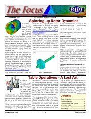
To restart an analysis, we click on Main Menu > Analysis Type > Restart. The 

following image shows a typical result of performing that operation: 





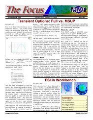
The white listing window shows us the available restart points for our analysis. In the 

case shown, we have a single restart point at load step 1, sub step 7. This corresponds to 

time 0.8 of our solution. We input the load step and sub step numbers for the desired 

restart point into the grey window, as shown. The action continue means that our 

analysis will attempt to progress with the solution. The other available actions are, end 

load step, and create results file. Typically we want our analysis to continue. 

The procedure to do a restart analysis is as follows: 

1. If you are still in ANSYS, leave the solution module and return to it by entering 

FINISH and then /SOLU or click on Main Menu > Finish or Main Menu > 

General Postproc and then return to Main Menu > Solution. 

2. Specify a restart analysis by issuing ANTYPE,,REST (Main Menu > Solution > 

Restart). 

3. Make the changes necessary to the loads, boundary conditions, solution options, 

etc. for the restart. For example, you can increase the number of substeps to 

enhance the convergence process, or change the loads to model a different loading 

condition. 





4. 

5. 

In case you used the Frontal solver (not the default), specify whether the 

triangularized matrix, jobname.tri, will be reused. See the documentation on the 

KUSE command for more information. 

Initiate the restart solution by issuing the SOLVE command. (Main Menu > 

Solution > Solve > Current LS). 

At this point, the solution will continue. Any results sets on the results file for load 

step/sub step/time points after the specified restart point will be deleted. If the restart 

solution is successful, new results sets will be added to the results file at the appropriate 

load step/sub step/time point indices. 

By default ANSYS will utilize the multi-frame restart files, which again will allow us to 

at least perform a restart from the last converged substep of the last load step. We can use 

RESCONTROL prior to the initiation of our first solution to specify more restart points. 

The drawback in specifying lots of restart points is that our restart files will take up more 

and more room on our hard disk. 

Note that for surface to surface contact elements, we must set KEYOPT(10) to 1 or 2 in 

order for the contact stiffness, FKN, to be changed between load steps or in a restart. 

This step is no longer necessary in ANSYS 7.0, however. 

An additional capability of the multi-frame restart is to add results sets to the results file. 

This can be done for load step/sub step/time points for which restart files have been 

written but for which no results were initially written to the results file. 

Restarts are useful in allowing us to explore a different load history than we originally 

planned as well as in recovering from an unconverged solution. We can hopefully make 

changes to our model to get a converged solution without having to run the entire 

solution again. 

More information can be found in the on-line Help System, in the Basic Analysis 

Procedures Guide, Section 3.16, entitled Restarting an Analysis. 





by Kurt Miller of Axel Products, Inc. 

Introduction 


The objective of the testing described herein is to define and to satisfy the input 

requirements of mathematical material models for elastomers that exist in 

ANSYS. 

The testing of elastomers for the purpose of defining material models is often 

misunderstood. The appropriate experiments are not yet clearly defined by 

national or international standards organizations. This difficulty derives from the 

complex mathematical models that are required to define the nonlinear and the 

nearly incompressible attributes of elastomers. 

Most of these models are referred to as hyperelastic material models and they 

include Mooney-Rivlin and Ogden models. However, most models share common 

test data input requirements. In general, stress and strain data sets developed by 

stretching the elastomer in several modes of deformation are required and fitted 

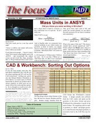
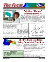
to sufficiently define the variables in the material models. A typical set of 3 stress 

strain curves appropriate for input into fitting routines is shown is shown in 

Figure 1. 





Figure 1. A Typical Final Data Set for Input into the ANSYS Curve Fitter. 

Testing in Multiple Strain States 

The modes of deformation each put the material into a particular state of strain. 

One objective of testing is to achieve pure states of strain such that the stress 

strain curve represents the elastomer behavior only in the desired state. The 

purpose of fitting multiple states of strain rather than just tension is that 

hyperelastic material models may easily create non-physical results in strain states 

not represented in the experimental data. 

For incompressible elastomers, the basic strain states are simple tension, pure 

shear and equal biaxial extension. For slightly compressible situations or 

situations where an elastomer is highly constrained, a volumetric compression test 

may be needed to determine the bulk behavior. 

Simple Tension Strain State 

The most significant requirement for simple tension is that in order to achieve a 

state of pure tensile strain, the specimen must be much longer in the direction of 

stretching than in the width and thickness dimensions. The objective is to create 

an experiment where there is no lateral constraint to specimen thinning. A 

non-contacting strain measuring device such as a video extensometer or laser 

extensometer is required to measure strain where the pure strain condition exists. 





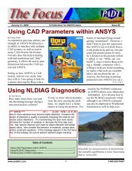
Figure 2. A Tension Experiment using a Video Extensometer. 

Pure Shear Strain State 

The pure shear experiment used for analysis is not what most of us would expect. 

The experiment appears at first glance to be nothing more than a very wide tensile 

test. However, because the material is nearly incompressible, a state of pure shear 

exists in the specimen at a 45-degree angle to the stretching direction. The most 

significant aspect of the specimen is that it is much shorter in the direction of 

stretching than the width. The objective is to create an experiment where the 

specimen is perfectly constrained in the lateral direction such that all specimen 

thinning occurs in the thickness direction. 





Figure 3. A Pure Shear Experiment using a Laser Extensometer. 

Equal Biaxial Strain State 

For incompressible or nearly incompressible materials, equal biaxial extension of 

a specimen creates a state of strain equivalent to pure compression. Although the 

actual experiment is more complex than the simple compression experiment, a 

pure state of strain can be achieved which will result in a more accurate material 

model. The equal biaxial strain state may be achieved by radial stretching a 

circular disc. 





Figure 4. A Biaxial Extension Experiment. 

Volumetric Compression 

Volumetric compression is an experiment where the compressibility of the 

material is examined. In this experiment, a cylindrical specimen is constrained in 

a fixture and compressed. The actual displacement during compression is very 

small and great care must be taken to measure only the specimen compliance and 

not the stiffness of the instrument itself. The initial slope of the resulting 

stress-strain function is the bulk modulus. This value is typically 2-3 orders of 

magnitude greater than the shear modulus for elastomers. 

Using Slow Cyclic Loadings to Create 

Stress Strain Curves 

The structural properties of elastomers change significantly during the first 

several times that the material experiences straining. This behavior is commonly 

referred to as the Mullins effect. If an elastomer is loaded to a particular strain 





level followed by complete unloading to zero stress several times, the change in 

structural properties from cycle to cycle as measured by the stress strain function 

will diminish. When the stress strain function no longer changes significantly, the 

material may be considered to be stable for strain levels below that particular 

strain maximum. 

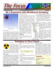
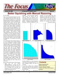
If the elastomer is then taken to a new higher strain maximum, the structural 

properties will again change significantly. One example of this behavior is shown 

in Figure 5 where an elastomers is strained to 20% strain for 10 repetitions 

followed by straining to 50% for 10 repetitions and followed by straining to 100% 

for 10 repetitions. 

Figure 5. Multiple Strain Cycles of an Elastomer at 3 Maximum Strain Levels. 

Observations 

Several observations can be made regarding this behavior that is true to a varying 

degree for all elastomers. 

1. The stress strain function for the 1st time an elastomer is strained is never 

again repeated. It is a unique event. 





2. 

3. 

4. 

5. 

The stress strain function does stabilize after between 3 and 20 repetitions 

for most elastomers. 

The stress strain function will again change significantly if the material 

experiences strains greater than the previous stabilized level. In general, the 

stress strain function is sensitive to the maximum strain ever experienced. 

The stress strain function of the material while increasing strain is different 

than the stress strain function of the material while decreasing strain. 

After the initial straining, the material does not return to zero strain at zero 

stress. There is some degree of permanent deformation. 

Limitations of Hyperelastic Material 

Models 

Most material models in commercially available finite element analysis codes 

allow the analyst to describe only a subset of the structural properties of 

elastomers. This discussion revolves around hyperelastic material models such as 

the Mooney-Rivlin and Ogden formulations and relates to those issues which 

effect testing. 

1. The stress strain functions in the model are stable. They do not change with 

repetitive loading. The material model does not differentiate between a 1st 

time strain and a 100th time straining of the part under analysis. 

2. There is no provision to alter the stress strain description in the material 

model based on the maximum strains experienced. 

3. The stress strain function is fully reversible so that increasing strains and 

decreasing strains use the same stress strain function. Loading and 

unloading the part under analysis is the same. 

4. The models treat the material as perfectly elastic meaning that there is no 

provision for permanent strain deformation. Zero stress is always zero 

strain. 

The Need for Judgment 

Because the models use a simple reversible stress strain input, one must input a 

stress strain function that is relevant to the to loading situation expected in the 

application. Naturally, this may be difficult because the very purpose of the 





analysis is to learn about the stress strain condition in the part. However, there are 

a few guidelines that may be considered. 

1. If the focus of the analysis is to examine the first time straining of an 

elastomeric part, then use the first time stress strain curves from material 

tests. This might be the case when examining the stresses experienced 

when installing a part for the first time. 

2. If the focus of the analysis is to understand the typical structural condition 

of a part in service, use stress strain curves derived by cycling a material 

until it is stable and extracting the stabilized increasing strain curve. 

3. If the focus of the analysis is to understand the unloading performance of a 

part in service by examining the minimum stress conditions, extract a 

stabilized decreasing strain curve. 

4. Perform experiments at strain levels that are reasonable for the application. 

Large strains that greatly exceed those that the part will experience will 

alter the material properties such that they are unrealistic for the application 

of interest. 

5. Stabilize the material at 2 or more different levels to cover a broader range 

of performance and to measure just how sensitive the structural properties 

are to maximum strain levels. 

Conclusion 

Physical testing of elastomers for the purpose of fitting material models in finite 

element analysis requires experiments in multiple states of strain under carefully 

considered loading conditions. The material models themselves have limitations 

and these limitations must also be considered. 

More technical downloads on the testing of plastics and elastomers may be found 

at: www.axelproducts.com/pages/Downloads.html. 





Axel Products, Inc. 

Testing Services 

Hyperelastic Properties of 

Elastomers 

Elastic Plastic Properties of 

Plastics 

Simple Tension, Pure Shear, Simple Shear 

Equal Biaxial Extension, Bulk 

Compression 

Data for: Ogden, Mooney-Rivlin, 

Arruda-Boyce 

Long Term Creep & Stress 

Relaxation 

Tension, Compresion and Shear 

Bulk Compression, Thin Films 

Determination Modulus, Poisson's 

Ratio, Yield Strains ... 

Data for: Elastic-Plastic, Orthotropic 

... 

Basic Thermal Properties 

Instrumented CSR 

Relaxation and Recovery Sequence 

Long Term Creep 

Dynamic & Viscoelastic Tests 

Dynamic Vibrations 

High Strain Rate Experiments 

Acoustic Frequency Experiments 

Static and Dynamic Component 

Tests 

Thermal Conductivity, Diffusivity 

Specific Heat 

Thermal Expansion and Glass 

Transition 

Durability and Crack Growth 

Static Tearing Energy 

Crack Growth under Dynamic 

Loadings 

Dynamic Characterization of Bushings 

Load-deflection with Imaging 

Friction 





The Focus is a periodic electronic publication published by PADT, aimed at the 

general ANSYS user. The goal of the feature articles is to inform users of the 

capabilities ANSYS offers and to provide useful tips and hints on using these 

products more effectively. The Focus may be freely redistributed in its entirety. 

For administrative questions, please contact Rod Scholl at PADT. 

The Focus Library 

All past issues of The Focus are maintained in an online library, which can be 

searched in a variety of different ways. 

Contributor Information 

Please dont hesitate to send in a contribution! Articles and information helpful to 

ANSYS users are very much welcomed and appreciated. We encourage you to 

send your contributions via e-mail to Rod Scholl. 

Subscribe / Unsubscribe 

To subscribe to or unsubscribe from The Focus, please visit the PADT 

e-Publication subscriptions management page. 

Legal Disclaimer 


Phoenix Analysis and Design Technologies (PADT) makes no representations 

about the suitability of the information contained in these documents and related 

graphics for any purpose. All such document and related graphics are provided as 

is without warranty of any kind and are subject to change without notice. The 

entire risk arising out of their use remains with the recipient. In no event, 

including inaccurate information, shall PADT be liable for any direct, 

consequential, incidental, special, punitive or other damages whatsoever 

(including without limitation, damages for loss of business information), even if 

PADT has been advised of the possibility of such damages. 

The views expressed in The Focus are solely those of PADT and are not 

necessarily those of ANSYS, Inc. 

http://www.padtinc.com/epubs/focus/common/end.htm [11/23/2004 4:47:53 PM]

The Focus - Issue 12 - PADT

Create successful ePaper yourself

Delete template?

Save as template?