Transient Options: Full vs. MSUP FSI in Workbench - PADT
Transient Options: Full vs. MSUP FSI in Workbench - PADT
Transient Options: Full vs. MSUP FSI in Workbench - PADT

You also want an ePaper? Increase the reach of your titles
YUMPU automatically turns print PDFs into web optimized ePapers that Google loves.
September 8, 2006 The Focus Issue 51<br />
September 8, 2006 A Publication for ANSYS Users Issue 51<br />
By Rod Scholl<br />
<strong>Transient</strong> <strong>Options</strong>: <strong>Full</strong> <strong>vs</strong>. <strong>MSUP</strong><br />
Ever try to do a transient analysis over a<br />
small time doma<strong>in</strong>… and get the feel<strong>in</strong>g<br />
maybe you’re us<strong>in</strong>g the wrong tool? Ever<br />
watch time march pa<strong>in</strong>fully forward <strong>in</strong> milliseconds<br />
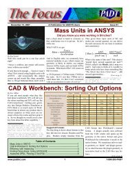
and still get spikey response<br />
curves out of /Post26 like this one?<br />
Perhaps you’ve overlooked the <strong>MSUP</strong> option<br />
on the TRNOPT command.<br />
TRNOPT,FULL – The Default<br />
The full transient analysis uses the force<br />
equation you might expect:<br />
And the ma<strong>in</strong> requirement is that one<br />
chooses time steps small enough to capture<br />
the system response (and of course required<br />
resolution on <strong>in</strong>put BC’s). If you’re not<br />
<strong>in</strong>terested <strong>in</strong> any response due to fundamental<br />
vibration modes… mean<strong>in</strong>g all your<br />
loads are applied at rates well below the<br />
first fundamental mode… then time step<br />
size probably isn’t that critical… But then<br />
aga<strong>in</strong>, why not just do a static solution<br />
given the quasi-static nature of the problem?<br />
More likely the first frequency of the system<br />
and hence its response is around or<br />
below the boundary condition <strong>in</strong>put frequency<br />
– which means one needs to take<br />
small time steps. When watch<strong>in</strong>g the l<strong>in</strong>es<br />
on the screen (see l<strong>in</strong>k on how) creep along,<br />
I f<strong>in</strong>d lots of time to do little calculations<br />
like this. A good m<strong>in</strong>imum rule is 8 po<strong>in</strong>ts<br />
on each ½ s<strong>in</strong> curve… or:<br />
1 / (highest frequency of <strong>in</strong>terest * 16)<br />
But then aga<strong>in</strong>… this is be<strong>in</strong>g quite skimpy.<br />
If the excitation is only expected to excite<br />
the lowest fundamental mode… then this<br />
might be doable depend<strong>in</strong>g on your problem<br />
def<strong>in</strong>ition. But if you need the 3rd<br />
mode… or 8th mode… or aren’t sure, and<br />
just need “as many as you can”… then we<br />
may be talk<strong>in</strong>g about A LOT of time<br />
steps… If your DOF count is high… this<br />
might take, well, way too long.<br />
TRNOPT,<strong>MSUP</strong><br />
The alternative is to use the Modal Superposition<br />
Method (TRNOPT,<strong>MSUP</strong>). This<br />
method first solves the mode shapes up to<br />
the specified highest response frequency of<br />
<strong>in</strong>terest. Then given an <strong>in</strong>put profile of<br />
BC’s <strong>in</strong> the time doma<strong>in</strong>, it is a simple<br />
matter of superposition to predict the response<br />
(handled <strong>in</strong>ternally <strong>in</strong> ANSYS with<br />
just a few commands). You can even take<br />
large time steps <strong>in</strong> regions of the time doma<strong>in</strong><br />
where you have little <strong>in</strong>terest. Read<br />
By Doug Oatis<br />
the theory manual to conv<strong>in</strong>ce yourself that<br />
this is more than just an approximation and<br />
will yield accurate predictions.<br />
Whats the catch?<br />
With <strong>MSUP</strong> one has to CHOOSE which<br />
higher modes to ignore. And by ignore…<br />
they just will not be present. If this mode is<br />
excited <strong>in</strong> your part, and it fails… they may<br />
come look<strong>in</strong>g for you.<br />
But with FULL method, one has to<br />
CHOOSE time step size. This thereby determ<strong>in</strong>e<br />
which responses are ignored, depend<strong>in</strong>g<br />
on the times step size used (if<br />
AUTOTS is off) or by the roll of the dice if<br />
one allows AUTOTS to by chance skip over<br />
peak responses. If the response curve is<br />
spiky as shown above, it will hopefully be<br />
noticed and more time po<strong>in</strong>ts requested…<br />
However, many peaks are just pla<strong>in</strong> stepped<br />
over and you are none the wiser. If the<br />
skipped response is excited and your part<br />
fails… they may come look<strong>in</strong>g for you.<br />
The difference here be<strong>in</strong>g with <strong>MSUP</strong> you<br />
can claim you didn’t have “time” or<br />
“budget” to <strong>in</strong>vestigate us<strong>in</strong>g the outdated<br />
8086 XT grafted on to the Tandy 1000<br />
motherboard they supplied you – whereas<br />
with FULL, the missed frequency of response<br />
will look less “deliberate” and therefore<br />
you will be burned by (Cont. on Pg. 2.)<br />
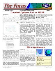
<strong>FSI</strong> <strong>in</strong> <strong>Workbench</strong><br />
One topic that hasn’t been discussed <strong>in</strong><br />
quite a while has been the <strong>FSI</strong> (Fluid-Structure<br />
Interaction) capability with<strong>in</strong> ANSYS<br />
<strong>Workbench</strong>. This article is aimed at describ<strong>in</strong>g<br />
a one-way analysis, where the<br />
pressure results are taken from CFX and<br />
mapped onto a structural analysis. If needed,<br />
a two-way analysis is available (with the<br />
appropriate license) where the fluid and<br />
structural doma<strong>in</strong>s are solved until both are<br />
<strong>in</strong> equilibrium.<br />
For a one-way <strong>FSI</strong> analysis, the underly<strong>in</strong>g<br />
assumption is that the deflections caused <strong>in</strong><br />
the structure do not signifi-<br />
(Cont. on Pg. 3.)<br />
Contents<br />
<strong>Full</strong> <strong>vs</strong>. <strong>MSUP</strong> ................................1<br />
<strong>FSI</strong> <strong>in</strong> <strong>Workbench</strong> ...........................1<br />
The Magic of PGR ..........................3<br />
Welcome to CFX.............................4<br />
4D Table Macro...............................5<br />
www.padt<strong>in</strong>c.com 1 1-800-293-<strong>PADT</strong>
September 8, 2006 The Focus Issue 51<br />
(<strong>Full</strong> <strong>vs</strong>. <strong>MSUP</strong>, Cont.)<br />
the angry mob of eng<strong>in</strong>eer non-believers.<br />
What’s the OTHER catch?<br />
Because the <strong>MSUP</strong> method requires a modal<br />
solution, the memory required for a given<br />
model is higher with <strong>MSUP</strong> than with the<br />
FULL method. I have found that if one has<br />
models this large, though, the FULL method<br />
is still prohibitive due to solve times for<br />
most common excitation pulses. And thus<br />
on today’s computers at least, speed and not<br />
memory is the limit<strong>in</strong>g factor on solv<strong>in</strong>g<br />
transients with small time steps.<br />
An example -Try this one: Note the listed<br />
solve times. (I have to admit this script is<br />
adapted from one I found on my computer,<br />
and I don’t know who the orig<strong>in</strong>al author<br />
was. So I thank you and apologize for not<br />
giv<strong>in</strong>g you credit.) Also, this wasn’t set up<br />
to skip a transient peak dur<strong>in</strong>g a run – but<br />
that would be an even stronger demonstration<br />
for the value of the <strong>MSUP</strong> method.<br />
Below is a test case that attempts to capture<br />
the response of frequencies of the first five<br />
modes.<br />
In this last case, the number of time steps<br />
was chosen to yield a solve time of 1.8 hrs<br />
to be equal to the <strong>MSUP</strong> method tested<br />
above. You can see what k<strong>in</strong>d of spikey<br />
response one gets for an equivalent solve<br />
time…<br />
You can download the files used at:<br />
ftp.padt<strong>in</strong>c.com/public/downloads/full_ms<br />
up.zip<br />
(<strong>FSI</strong>, Cont.)<br />
cantly impact the fluid doma<strong>in</strong>. One example<br />
is the pressurization of an actuator cap,<br />
seen below.<br />
To beg<strong>in</strong>, you must first create the fluid<br />
doma<strong>in</strong> volume and mesh. Design Modeler<br />
is an excellent choice to do this with its Fill<br />
and Enclosure utilities. After the volume is<br />
created, you can use Simulation, CFX-<br />
Mesh, or ICEM-CFD to create the mesh.<br />
For the novice fluid mesher (of which I<br />
consider myself), Simulation or CFX-Mesh<br />
are the best choices. For the power-meshers<br />
out there, ICEM is your song.<br />
If you use CFX-Mesh or ICEM, you can<br />
create named selections/parts out of the<br />
surfaces that <strong>in</strong>terface with the solid and<br />
pass them to CFX-Pre. For this example, I<br />
only looked at the stresses <strong>in</strong> the cap, so I<br />
made a named selection out of all the surfaces<br />
that match up with the cap.<br />
After you’ve solved the fluid doma<strong>in</strong>, you<br />
can post-process as usual. Once you’re<br />
ready to solve the structural, you can reopen<br />
Design Modeler and prep the geometry<br />
for the structural analysis. For this example,<br />
I removed the p<strong>in</strong>-holes on the<br />
actuator cap, and suppressed out all bodies<br />
except for the cap.<br />
Once you br<strong>in</strong>g the geometry <strong>in</strong>to Simulation,<br />
go through your normal setup (i.e.<br />
def<strong>in</strong>e material properties, specify mesh<br />
controls, etc.). When you’re ready to load<br />
the part, simply apply a pressure to all the<br />
faces that match up to your fluid doma<strong>in</strong>. In<br />
the details w<strong>in</strong>dow for the pressure, change<br />
the ‘Constant’ to be ‘CFX Results’. You’ll<br />
then be prompted to select the result file<br />
(filename.res), region, and time step (if<br />
applicable). The regions will be listed for<br />
every surface that you have applied a<br />
boundary condition <strong>in</strong> CFX. For this example,<br />
I manually applied a wall BC to the <strong>FSI</strong><br />
faces (even though all unconstra<strong>in</strong>ed faces<br />
have a wall applied to them). This enabled<br />
me to easily pick the region of the CFX<br />
model to pull the pressures from.<br />
After you specify the result file, region, and<br />
time step, <strong>Workbench</strong> will go off and <strong>in</strong>terpolate<br />
the pressures onto the structural face.<br />
You’ll see 3 static isotropic pictures appear<br />
below the ‘Pressure’ <strong>in</strong> the tree. These will<br />
show the pressure values <strong>in</strong>terpolated from<br />
the CFX model. After you solve the model,<br />
you’ll see an additional 3 pictures show<strong>in</strong>g<br />
the pressures applied to the structural model.<br />
With a decent mesh, you should see the<br />
exact same pictures on both the CFX and<br />
Structural side.<br />
So now you’re probably th<strong>in</strong>k<strong>in</strong>g, “Well,<br />
that’s great, but what does this really do for<br />
me?” The short answer is that it allows you<br />
to better simulate your environment. Instead<br />
of assum<strong>in</strong>g some sort of pressure<br />
distribution, you can use the actual gradient<br />
and better simulate reality. One th<strong>in</strong>g you<br />
must always keep <strong>in</strong> m<strong>in</strong>d, however, is to<br />
(Cont. on Pg. 3.)<br />
www.padt<strong>in</strong>c.com 2 1-800-293-<strong>PADT</strong>
September 8, 2006 The Focus Issue 51<br />
(<strong>FSI</strong>, Cont.)<br />
make sure you’re apply<strong>in</strong>g the proper pressure<br />
differential across the part. You need<br />
to make sure that the pressure calculated<br />
from CFX-Post represents absolute pressure.<br />
If not, you will need to pressurize the<br />
outer portion of your model to get the proper<br />
delta.<br />
The two-way <strong>FSI</strong> analysis is a bit more<br />
complicated, requir<strong>in</strong>g ANSYS Classic<br />
knowledge <strong>in</strong> order to setup the Fluid and<br />
Structural <strong>in</strong>terfaces (so each solver can<br />
pass <strong>in</strong>fo back and forth). The setup for this<br />
analysis should become easier <strong>in</strong> future<br />
releases as more ANSYS technologies are<br />
brought underneath the <strong>Workbench</strong> <strong>in</strong>terface.<br />
Faster Results from Smaller<br />
Files: The Magic of PGR<br />
By Eric Miller<br />
Did you ever get frustrated by how long it<br />
sometimes takes to make a large and complex<br />
plot <strong>in</strong> ANSYS? Did you wonder why<br />
ANSYS has never done anyth<strong>in</strong>g to speed<br />
up plott<strong>in</strong>g and create smaller results files?<br />
Well guess what, they did do someth<strong>in</strong>g<br />
years ago but most users don’t know it is<br />
there or have not made it a habit to use. The<br />
secret is the PGR file and a set of commands<br />
created to use it.<br />
Standard and Power Graphics<br />
Before delv<strong>in</strong>g <strong>in</strong> to the PGR file, it is a<br />
good idea to look at why the RST files that<br />
ANSYS makes are so big and why plots<br />
take so long. The answer is actually pretty<br />
simple and when you th<strong>in</strong>k about it, makes<br />
sense and like a lot of th<strong>in</strong>gs falls under the<br />
old 80-20 rule. Approximately 80% (+/-<br />
15% or so depend<strong>in</strong>g on your actual needs)<br />
of the time users are plott<strong>in</strong>g nodal result<br />
values on the external surface of their models.<br />
But, sometimes you need to have <strong>in</strong>ternal<br />
<strong>in</strong>formation, you want to do the nodal<br />
averag<strong>in</strong>g differently, you want to look at<br />
results on a per-element basis, or you want<br />
to calculate the quality of your model by<br />
look<strong>in</strong>g at the variation <strong>in</strong> results from element<br />
to element. For the 20% of the time<br />
you need to have the result that ANSYS<br />
calculated for each element at each node on<br />
the element.<br />
To understand this better th<strong>in</strong>k back to what<br />
happens <strong>in</strong> a solve. The program solves for<br />
the displacement of each node (DOF), then<br />
uses those values at each node <strong>in</strong> each element<br />
to calculate a stress and stra<strong>in</strong> for that<br />
node and that element based upon the formulation<br />
and material properties of the element.<br />
ANSYS stores the results for each<br />
node <strong>in</strong> each element <strong>in</strong> the result file. A<br />
s<strong>in</strong>gle nodal value for each node is not calculated<br />
until the user requests a plot. When<br />
this happens, the program must read the<br />
element based nodal results, average over<br />
each element that shares a given node, then<br />
store the result<strong>in</strong>g value <strong>in</strong> memory.<br />
So, the RST file is bigger than one would<br />
expect because each element stores results<br />
for each node on the element. If a node is<br />
shared by six elements, all the stress and<br />
stra<strong>in</strong> <strong>in</strong>formation is stored six times! Also,<br />
all that data must be read <strong>in</strong>to memory,<br />
sorted, averaged by node number, then plotted.<br />
That takes time and memory and is<br />
repeated for every plot.<br />
So to save memory and time, ANSYS <strong>in</strong>troduced<br />
the PowerGraphics option many<br />
years ago. This changed the averag<strong>in</strong>g algorithm<br />
to only look at nodes on the surface<br />
of an object when do<strong>in</strong>g the averag<strong>in</strong>g. This<br />
reduced the amount of memory required<br />
and speeds up the averag<strong>in</strong>g calculation. It<br />
also, as most of you should have noticed by<br />
now, produces different results (search<br />
powergraphics at www.xansys.net).<br />
Solv<strong>in</strong>g the Time and File Issue<br />
After <strong>in</strong>troduc<strong>in</strong>g Power-<br />
(Cont. on Pg. 4.)<br />
Advantages &<br />
Disadvantages of<br />
PowerGraphics?<br />
Even if you don’t use the PGR file,<br />
you can change the default plott<strong>in</strong>g to<br />
or from PowerGraphics with the<br />
/GRAPHICS command. When us<strong>in</strong>g<br />
this option you can realize the follow<strong>in</strong>g<br />
advantages:<br />
Faster plott<strong>in</strong>g<br />
Curved element edges on quadratic<br />
elements<br />
Captures discont<strong>in</strong>uity from different<br />
materials<br />
Displays top and bottom stresses on<br />
shells at the same time<br />
Allows use of Query command to<br />
pick and see results on elements<br />
But there are some drawbacks:<br />
Does not work for circuit elements<br />
Averag<strong>in</strong>g only uses elements with<br />
faces on the surface<br />
M<strong>in</strong> and Max values are for surface<br />
elements only<br />
No element coord<strong>in</strong>ate system plott<strong>in</strong>g<br />
To understand how stresses change,<br />
look at the example below. To get the<br />
stresses on the top surface: <strong>in</strong> full<br />
graphics, stress from the green and red<br />
dotted element corners are averaged.<br />
For PowerGraphics, only the green dotted<br />
ones are used.<br />
www.padt<strong>in</strong>c.com 3 1-800-293-<strong>PADT</strong>
September 8, 2006 The Focus Issue 51<br />
Graphics, the next logical step was to bypass<br />
the RST file and store the<br />
PowerGraphics <strong>in</strong>formation <strong>in</strong> a file dur<strong>in</strong>g<br />
the solve. Now you have a much smaller<br />
file, your averag<strong>in</strong>g is done only once, and<br />
you need a lot less memory.<br />
To use this file you simply need to<br />
tell ANSYS to create the PGR file<br />
dur<strong>in</strong>g a solve, or if you forget<br />
about the command and want to do<br />
it after you have solved, you can<br />
generate a PGR file from a result<br />
file. The easiest way to do this is to<br />
use the GUI as shown <strong>in</strong> Figure 1.<br />
From the GUI you can see all the<br />
options that are available to you<br />
through the GUI or the PGWRITE<br />
command. Look<strong>in</strong>g at these commands<br />
you can see that the PGR file<br />
offers a lot of control.<br />
First off, you can specify the filename.<br />
This way you can do th<strong>in</strong>gs<br />
like create a separate file for each<br />
load step or, if you are us<strong>in</strong>g the command<br />
to extract key <strong>in</strong>fo from an exist<strong>in</strong>g RST<br />
file, you can create a PGR for each type of<br />
result data you want to store.<br />
This is often done by chang<strong>in</strong>g the sett<strong>in</strong>gs<br />
on the next option, which controls the type<br />
of results to store. S<strong>in</strong>ce users usually only<br />
By: J Luis Rosales, PhD<br />
<strong>PADT</strong> has had the privilege of work<strong>in</strong>g<br />
with the world-class CFD program, CFX,<br />
for the past three years. Dur<strong>in</strong>g this time,<br />
we have solved small and simple models of<br />
a few thousand nodes to large and complex<br />
models with many millions of nodes.<br />
Before mov<strong>in</strong>g onto specific <strong>in</strong>struction,<br />
such as import<strong>in</strong>g a mesh from another tool<br />
(a good topic for a future article) let’s start<br />
with a CFX overview.<br />
want stress results, choos<strong>in</strong>g only that option<br />
can make the file much smaller.<br />
By default, the PGR file only uses average<br />
nodal values on the surface of your model.<br />
But if you need the <strong>in</strong>ternal <strong>in</strong>formation you<br />
can set it with the next option. You can also<br />
tell ANSYS to store unaveraged data,<br />
although do<strong>in</strong>g so k<strong>in</strong>d of destroys the<br />
po<strong>in</strong>t of us<strong>in</strong>g the PGR file. Lastly,<br />
you can tell the program to only store<br />
the <strong>in</strong>ternal <strong>in</strong>formation that is required<br />
for special plots like sections<br />
and vectors. This is a lot less data<br />
than the <strong>in</strong>ternal nodal <strong>in</strong>formation.<br />
Although it is much more efficient to<br />
create the file as part of the solution,<br />
you can always create it from an exist<strong>in</strong>g<br />
results file <strong>in</strong> POST1. When do<strong>in</strong>g<br />
so you should be aware of a few<br />
th<strong>in</strong>gs. First, you need to do a SET<br />
and a PGWRITE for each result set<br />
you want to store. Second, the results<br />
are stored <strong>in</strong> the current result coord<strong>in</strong>ate<br />
system (RSYS).<br />
To use your PGR file you need to tell AN-<br />
SYS to not use the RST and po<strong>in</strong>t it to your<br />
smaller file with PGRPH,ON. Also, to get<br />
at different results sets, you simply use the<br />
PGRSET command <strong>in</strong>stead of the SET<br />
command. And, if you want to look at a<br />
subset of nodes <strong>in</strong> the PGR file, use the<br />
PGSELE command. That is about it.<br />
How much Better is it?<br />
To get a feel for the difference, we dusted<br />
off our handy-dandy generic low pressure<br />
turb<strong>in</strong>e disk and blade model (shown to the<br />
left as eye candy for the otherwise dull<br />
article) and did a static stress solution on it<br />
with PGWRITE turned on. Here are some<br />
statistics:<br />
Number of Nodes: 399,870<br />
Number of Elements: 268,507<br />
RST files size:<br />
PGR file size:<br />
Plot RST:<br />
ANSYS CFX: Welcome to CFX<br />
CFX is composed of three modules similar<br />
to the ANSYS architecture: CFX-Pre (a<br />
preprocessor), CFX-Solver (the solution<br />
solver) and CFX-Post (a post processor).<br />
These modules are started from a CFXlauncher<br />
w<strong>in</strong>dow. CFX-Pre assumes you<br />
already have a meshed model and does not<br />
create the mesh. It is basically used to<br />
def<strong>in</strong>e the problem, apply boundary conditions<br />
and set up a few solver sett<strong>in</strong>gs.<br />
CFX-Solver takes a *.def file created by<br />
CFX-Pre and solves the model to produce a<br />
solution. CFX-Solve can be as easy as<br />
click<strong>in</strong>g the solve button for a simple serial<br />
run to sett<strong>in</strong>g up a large distributed run for<br />
a multi-million node model. CFX-Post is<br />
easily one of the best post-process<strong>in</strong>g tools<br />
that we have used for CFD results. The<br />
regular CFX tutorials do a very nice job of<br />
<strong>in</strong>troduc<strong>in</strong>g users to the features available <strong>in</strong><br />
CFX-Post; however, some <strong>in</strong>formation that<br />
may be of <strong>in</strong>terest to users may be covered<br />
<strong>in</strong> future Focus articles. Also, CFX is a<br />
more advanced tool than the FLTORAN<br />
CFD code available <strong>in</strong> ANSYS. Flotran is<br />
of course still available.<br />
So pull out the CFX <strong>in</strong>stallation files, get a<br />
temp license from your ASD (if necessary)<br />
– and poke around the <strong>in</strong>terface of this new<br />
member to the ANSYS family.<br />
615,120 MB<br />
50,790 MB<br />
8.3 msec<br />
Plot PGR:<br />
5.5 msec<br />
Faster, Smaller is Better<br />
The first th<strong>in</strong>g that the data above po<strong>in</strong>ts out<br />
is that computers have gotten so fast (we ran<br />
on a DUAL Opteron with 8GB of RAM)<br />
that the speed difference for a fairly normal<br />
model is small. But for larger models the<br />
difference becomes significant, and the files<br />
size change is significant.<br />
So, next time you start grumbl<strong>in</strong>g about<br />
shuffl<strong>in</strong>g around multi-gigabyte RST files,<br />
remember the lowly PGR file and give it a<br />
try.<br />
www.padt<strong>in</strong>c.com 4 1-800-293-<strong>PADT</strong>
September 8, 2006 The Focus Issue 51<br />
Awesome APDL: Writ<strong>in</strong>g a 4D Table to a File<br />
This month’s APDL macro is a nice example<br />
of how to write data from a four dimensional<br />
array to a text file. It was created<br />
because a customer needed to <strong>in</strong>terpolate<br />
data based on X, Y, Z position and time.<br />
Once they made their table they wanted to<br />
store it <strong>in</strong> a text file for review.<br />
On first glance a simple task but it turns out<br />
that you need someth<strong>in</strong>g special because the<br />
*MWRITE command only handles three<br />
dimensional arrays. So the solution is to<br />
write a 3D array for each of the fourth<br />
dimensions.<br />
This clever solution also shows how you<br />
can use the *cfwrite command to have a<br />
macro create a macro. This is how you can<br />
do text replacement on commands that<br />
don’t support it outwrite, like the *vwrite<br />
command. In this case, we use it so the<br />
name of the table can be a variable.<br />
Enjoy, and notice that we avoided the use of<br />
a tacky Twilight Zone joke...<br />
*dim,tabled,tab4,5,3,2,2<br />
! Loop on each dimension,<br />
! fill<strong>in</strong>g the table with some data<br />
*do,i,0,5<br />
*do,j,0,3<br />
*do,k,1,2<br />
*do,l,1,2<br />
tabled(i,j,k,l)=i+10*j+100*k+1000*l<br />
*enddo<br />
*enddo<br />
*enddo<br />
*enddo<br />
! Get a name from the user<br />
*ask,tab_name,Enter Table<br />
name,'tabled'<br />
!>>>> END OF PART1<br />
! Part 2 works on a table def<strong>in</strong>ed<br />
! by tab_name and can be<br />
! used <strong>in</strong> a generic way<br />
!<br />
! dimension size for<br />
*get,d_tabi,parm,%tab_name%,dim,x<br />
*get,d_tabj,parm,%tab_name%,dim,y<br />
*get,d_tabk,parm,%tab_name%,dim,z<br />
*get,d_tabl,parm,%tab_name%,dim,4<br />
k=1<br />
! Open a file to create the writ<strong>in</strong>g<br />
macro <strong>in</strong><br />
*cfopen,dtable,mac<br />
! write out the command for<br />
! writ<strong>in</strong>g stuff<br />
*vwrite<br />
('*mwrite,%arg1%(0,0,k,l),d_test-<br />
%arg2%,txt')<br />
! Write out the format <strong>in</strong>fo<br />
*do,i,1,d_tabj+1<br />
*vwrite<br />
('%10.4F '$)<br />
*enddo<br />
! Done creat<strong>in</strong>g macro<br />
*cfclose<br />
!Loop on 4th dimension, call<strong>in</strong>g<br />
! the macro you made<br />
*do,l,1,d_tabl<br />
dtable,tab_name,l<br />
*endd<br />
There have been lots of improvements to contact <strong>in</strong> recent years. Sheldon Imaoka shares a great<br />
PowerPo<strong>in</strong>t that summarizes everyth<strong>in</strong>g at: ansys.net/ansys/papers/nonl<strong>in</strong>ear/contact_tech.pdf<br />
Ever thought about work<strong>in</strong>g for ANSYS, Inc? They have some nice jobs open right now. To see<br />
what is open, visit: ansys.recruitmax.com/candidates/default.cfm?szCategory=joblist<br />
Resources<br />
Upcom<strong>in</strong>g Tra<strong>in</strong><strong>in</strong>g Classes<br />
Month Start End # Title Location<br />
Sep ‘06 7-Sep 8-Sep 301 Heat Transfer Albq, NM<br />
11-Sep 13-Sep 101 Introduction to ANSYS, Part 1 Tempe, AZ<br />
18-Sep 21-Sep 802 Advanced APDL & Custom. Tempe, AZ<br />
25-Sep 26-Sep 201 Basic Structural Nonl<strong>in</strong>earities Tempe, AZ<br />
27-Sep 28-Sep 204 Adv. Contact and Bolt Pret. Tempe, AZ<br />
Oct ‘06 2-Oct 4-Oct 101 Introduction to ANSYS, Part 1 Albq. NM<br />
5-Oct 6-Oct 203 Dynamics Tempe, AZ<br />
9-Oct 10-Oct 100 Eng<strong>in</strong>eer<strong>in</strong>g with FE Analysis Irv<strong>in</strong>e, CA<br />
16-Oct 18-Oct 104 ANSYS <strong>Workbench</strong>, Intro Albq, NM<br />
19-Oct 19-Oct 105 ANSYS <strong>Workbench</strong>, Struc NL Albq, NM<br />
25-Oct 27-Oct 902 Multiphysics for MEMS Tempe, AZ<br />
Nov ‘06 1-Nov 3-Nov 101 Introduction to ANSYS, Part 1 Tempe, AZ<br />
8-Nov 9-Nov 107 ANSYS WB DesignModeler Tempe, AZ<br />
13-Nov 14-Nov 301 Heat Transfer Irv<strong>in</strong>e, CA<br />
16-Nov 17-Nov 102 Introduction to ANSYS, Part 2 Tempe, AZ<br />
27-Nov 28-Nov 604 Introduction to CFX Tempe, AZ<br />
L<strong>in</strong>ks<br />
News<br />
MatWeb now supports the creation of <strong>Workbench</strong> XML<br />
material files. Visit www.matweb.com to see <strong>PADT</strong>’s<br />
favorite on-l<strong>in</strong>e material repository<br />
Want to know which third party vendors are partnered<br />
with ANSYS, Inc? Visit<br />
www.ansys.com/corporate/partnerships.asp for a summary<br />
- Ch<strong>in</strong>a chooses ANSYS as standard <strong>in</strong> national<br />
eng<strong>in</strong>eer<strong>in</strong>g exam l<strong>in</strong>k<br />
- More Great F<strong>in</strong>ancial News:<br />
Highly Successful Second Quarter<br />
Name as Fortune Small Bus<strong>in</strong>ess Fastest<br />
Grow<strong>in</strong>g Companies for Third Consecutive<br />
Year l<strong>in</strong>k<br />
The Focus is a periodic publication of Phoenix Analysis & Design Technologies (<strong>PADT</strong>).<br />
Its goal is to educate and enterta<strong>in</strong> the worldwide ANSYS user community. More <strong>in</strong>formation<br />
on this publication can be found at: http://www.padt<strong>in</strong>c.com/epubs/focus/about<br />
www.padt<strong>in</strong>c.com 5 1-800-293-<strong>PADT</strong>
September 8, 2006 The Focus Issue 51<br />
www.padt<strong>in</strong>c.com 6 1-800-293-<strong>PADT</strong>