Be a Superhero with Workbench Scripting Radiation is Your ... - PADT

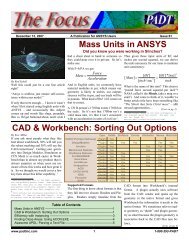
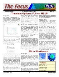
November 3, 2006 The Focus Issue 53 

November 3, 2006 A Publication for ANSYS Users Issue 53 

By Doug Oatis 

Be a Superhero with Workbench Scripting 

As a continuation to last month’s riveting 

article about beam modeling, I decided to 

dive into something a little more mysterious 

about Workbench – Customization and 

Scripting. As many of you know, you can 

still use APDL in command snippets in 

Workbench, but if you want to run macros 

interactively in Workbench, you need to 

By Rod Scholl 

It turns out it’s pretty 

easy to add radiation to a 

thermal model. The help 

manual can be very helpful 

in this area (as usual) 

but it leaves out the pep 

talk that indicates how easy it is to implement. 

Also, I just think radiation is neato 

and I look for any excuse I can to include it. 

When to add it? 

The implementation effort is just about the 

same as adding convection, except there is 

an impact on solve time given its highly 

non-linear nature. If you have a transient 

analysis, this impact will be negligible. If 

you are doing a steady state analysis, it 

might take 20 solves to reach a solution, 

thereby making a 20X impact on solution 

times. Yet, given that thermal models don’t 

require much mesh density and only have 1 

write them in JScript. 

I’ll take this moment right now to admit that 

I am not a computer science person. I took 

a couple of years of C++ in high school, 

played around with Python, and I know a 

little HTML. I’m probably most adept at 

using APDL, in fact, I would have been 

happy had the April Fool’s article 

about ANSYS buying Windows 

and rewriting the source 

code in APDL been true. All 

things considered, I’ve found 

JScript to be different, but not 

terribly difficult to learn. So this 

will hopefully be the beginning 

to a couple of articles about 

scripting in Workbench. A good 

JScript reference is the MS’s 

JScript Tour. 

Some quick notes that I’ve 

picked up through my JScripting 

journey: 

DOF per node, this often isn’t a problem 

either. 

Try a quick hand-calc of the heat load compared 

to your input loads to see how significant 

the impact of radiation is in your 

case. 

A is the area 

is the emissivity (somewhere between 0 

and 1) 

T is the temperature (must be in absolute 

so add 273 to your Celcius temps to get to 

kelvin, or 460 to your farenheits to get 

Rankine) 

is the Stefan Boltzman constant: 

0.119E-10 Btu/hr/in2/°R4 

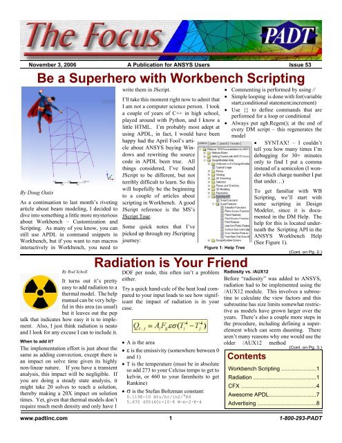
Figure 1: Help Tree 

Radiation is Your Friend 

Commenting is performed by using // 

Simple looping is done with for(variable 

start;conditional statement;increment) 

Use {} to define commands that are 

performed for a loop or conditional 

Always put agb.Regen(); at the end of 

every DM script – this regenerates the 

model 

SYNTAX! – I couldn’t 

tell you how many times I’m 

debugging for 30+ minutes 

only to find I put a comma 

instead of a semicolon (I wonder 

which charge number I put 

that under…) 

To get familiar with WB 

Scripting, we’ll start with 

some scripting in Design 

Modeler, since it is documented 

in the DM Help. The 

help for this is located underneath 

the Scripting API in the 

ANSYS Workbench Help 

(See Figure 1). 

Radiosity vs. /AUX12 

Before “radiosity” was added to ANSYS, 

radiation had to be implemented using the 

/AUX12 module. This involves a subroutine 

to calculate the view factors and this 

subroutine has size limits somewhat restrictive 

as models have grown larger over the 

years. There’s also a couple more steps in 

the procedure, including defining a superelement 

which can seem daunting. There 

aren’t many reasons why one would use the 

older /AUX12 method 

Contents 

(Cont. on Pg. 2.) 


Workbench Scripting ......................1 

Radiation ........................................1 

CFX ................................................4 

Awesome APDL..............................7 

Advertising ......................................8 

www.padtinc.com 1 1-800-293-PADT


(Scripting, Cont.) 

What I read in the help dealt with ‘Line 

from Points Feature’. There is a sample 

script listed, and you can learn a bit by 

reading it after reviewing some JScript basics. 

What I did with this script is take it 

and supercharge it (well, not really) using 

looping and conditional statements to automatically 

build up major portions of a beam 

derrick. 

The only prerequisite for making this script 

is consistency in creating your point file. 

For my example, I created a 5-tier derrick 

with a point at each corner. This allows 

easing looping to build up the legs (vertical 

beams) and each horizontal tier. The only 

user input required is to specify how many 

tiers and legs there are. 

Without further delay, here’s my script: 

1 Define a “Points from File” object, give 

it a name, and specify the file location 

(the file used is also available on the ftp 

site). Make sure to update the file location 

on the 3rd line 

2 Specify how many groups (horizontal 

sections) and how many legs 

3 Create a “Lines from Point” object and 

loop through the groups joining the 

same point number together 

4 Create another “Lines from Point” object, 

specify operation as add frozen, 

and the loop through and join sequential 

points together in each group. 

You’ll notice that I regenerate after every 

operation. Also, notice that I have j=2 for 

larger loop for the level creation. This is 

because I decided I didn’t want to create a 

beam level on the “ground”. Also notice the 

if statement so I can join Point 4 to Point 1. 

To run, simply go File > Run Script in 

Design Modeler. You should see the model 

shown at the start of the article (Minus the 

Superhero) Now you can go and impress 

your friends! 

You can download a copy of the script and 

input files from: 

ftp.padtinc.com/public/downloads/DM_pnt 

_bm_script.zip . 

doug_point=agb.FPoint(agc.FPointConstruction, 

agc.FPointCoordinateFile); 

doug_point.Name="DougsFile"; //Watch syntax on naming 

doug_point.CoordinateFile="D:\\ANSYS\\Tower3.txt"; 

// Change for your File 

agb.Regen(); 

group_num=5; 

num_legs=4; 

var dp1; 

var dp2; 

//Time to make the legs in one operation 

d_line=agb.LinePt(); 

d_line.Name="Legs"; 

for(j=1;j


(Radiation, Cont.) 

rather than the new “Radiosity” method… 

but both are supported. Some people find 

that /AUX12 is easier to achieve convergence 

in radiation-dominated problems. 

However, for larger models, if you use 

/AUX12 expect 20gb view factor files and 

loooong pauses during calculation of the 

viewfactor matrix where you will all but 

swear the code is crashed… just keep waiting. 

Also, I suspect there is residual stigma 

against implementing radiation because of 

the slightly more complicated /AUX12 procedure, 

whereas Radiosity is easier. 

These example scripts should come in 

handy if you are new to radiation. 

tradiation.mac: 

Radiation with Radiosity Solver (No 

Space Node) 

tspacenode3d.mac: 

Radiation with Radiosity Solver and 

Space Node 

tradaux12.mac: 

Radiation with /AUX12 method 

tradiation2d.mac: 

Radiation with Radiosity Solver (No 

Space Node) 2D 

tspacenode.mac: 

Radiation with Radiosity Solver and 

Space Node 2D 

To implement Radiosity, you simply apply 

a surface effect boundary condition (SF, 

SFA, SFL, etc.) directly on the element or 

geometry (or on a surface effect element 

like SURF152) – and specify an enclosure 

number. This enclosure number groups 

surfaces into sets where radiation is only 

evaluated for surfaces with the same enclosure 

number – this is similar to using REAL 

ID’s to define which contacts elements 

should be paired. You can always group all 

surfaces into a single enclosure, but on big 

models you might gain some time by breaking 

them up into sets and thereby making 

the view factor calculation less expensive. 

To implement the AUX12 method, you are 

basically building the view factors as a 

MATRIX50, and a different method to calculate 

form factors. This form factor matrix 

is read in as a superelement. (Note that 

there is no expansion pass, because there 

are no DOF’s in this element.) 

View Factor Calculation 

The AUX12 method on an element-by-element 

basis checks for the portion of the 

surface visible to one-another and thereby 

arrives at an AREA*Emmisivity value for 

each element combination as a percentage 

(0 to 1) of the total hemisphere visible to the 

element. 

As you may guess this is numerically intensive 

as element count grows. Using the 

older /AUX12 method you will have to 

specify a number of rays via the VTYPE 

command. The larger the number, the more 

computational time required. A couple 

times when I’ve varied the number I found 

that the default of 20 for 3-D still loses a 

little more accuracy than I’d prefer, and 

generally I use the maximum of 100. This 

is more computationally expensive, but not 

dramatically so… seems that once you are 

up to 20 rays, its easier to add more without 

too much expense. You might want to try 

two different values, like 20 and 30, and 

convince yourself that your number of rays 

is sufficient. Many folks just stick with the 

default, which in most cases is fine. 

With the radiostiy method, a cube rather 

than a sphere is used for the projecting 

surface, for which the manual, and several 

web resources dig into the theory on the 

minor loss in accuracy. Luckily you don’t 

need to understand any of this to implement 

it. In this case I also use an option of 100 

rather than the default of 10… but maybe 

I’m just paranoid to get the last 1% of error 

out of an analysis. 

You can always view the created matrix, via 

VFOPT or WRITE – which can be a fun 

exercise to take a couple elements and compare 

a quick hand-calc to the computed 

view factor. 

Emissivities 

Knowing the emissivity of a surface is often 

tricky. For all the accuracy I add with high 

ray tracing numbers, its probably made 

moot by the inaccuracy of most emmisivity 

numbers. Expect poor sources for emisivities 

– and note that oxidation and other 

factors often change the emissivity of a 

surface over product life. Further, surfaces 

actually have different emissivites (or absorbtions) 

for different ranges of the spectrum. 

Thus a single emissivity number is an 

approximation suited for many applications 

– but if you are dealing with radiation dominated 

problems with non-black body 

sources (meaning the whole spectrum isn’t 

being emitted or absorbed for material reasons) 

you will need a different tool than 

ANSYS such as CFX. 

Space Node 

As you expect the energy should balance. 

A space node is often used for this. For all 

the rays that don’t see another element, this 

exchange can be assigned to a space node. 

The advantage of this is one can specify the 

temperature nonzero of space. This can be 

0 Kelvin, if it’s truly radiating to “space” 

but more often you might choose a 

“background” temperature to represent the 

unmodeled portion of the system – such as 




(Radiation, Cont.) 

the outer shell of an engine, or room temperature. 

A nice advantage of the space node, given 

that you assign a DOF temperature to it, is 

you can check reaction loads at that node, 

and energy balance to see what amount of 

energy is leaking into space. Without a 

spacenode, you have to assume the missing 

energy went to space, but you will not ahve 

a verifiable way to account for this. In my 

experience a space node never hurts, and is 

defined with just three commands, 

N,800000 

!or some other unused node number 

SPCNOD,1,80000 

!for enclosure 1 

D,80000,temp,50 

!for 50 degree space temperature. 

Note, that a space node is one of those rare 

cases where no element must be associated 

with the node. 

Getting Convergence 

Because of the T*4 nonlinearity, convergence 

isn’t necessarily a breeze, although in 

most cases it’s trivial. ANSYS provided a 

few different methods for doing this, but I 

prefer the transient method. The other 

methods (such as QSOPT) are actually automated 

versions of this technique, so they 

are no faster, or more stable, just saves you 

By J. Luis Rosales, PhD 

typing a few commands. 

Basically, you will specify a starting temperature 

(such as IC,ALL,TEMP,700), and 

then run a transient analysis for it to reach 

steady-state. You will have to plot your 

results (in /POST26) to verify that you have 

reached near-equilibrium. The pic below 

shows a run perhaps terminated a little 

soon, but its up to the analyst the accuracy 

needed. 

For particularly hairy radiation problems 

you might not be able to chose a uniform 

starting temperature that yields convergence. 

This has been the rare case for me, 

but when encountered, I make intelligent 

guesses for a few different regions. In an 

extreme case, this too does not converge, 

and I first run a steady state conduction 

solution on my initial condition guesses 

(without radiation present) then add radiation 

and resolve. Something about the 

smooth temperature gradients eases convergence. 

Likely none of this will matter to 

you and a single IC command at ANY 

temperature will do the trick. You also 

might find that the /AUX12 converges more 

readily than radiosity, so you can always go 

back to that. 

Strange Brew: 

I can’t let an article on radiation go by 

without a nod to the film “Strange Brew’ 

(http://www.imdb.com/title/tt0086373/). 

Or more accurately the film within the film 

Strange Brew: 

Bob McKenzie: Fleshy-headed mutant. Are 

you friendly? 

Doug McKenzie: No way, eh? Ra-... radiation 

has made... me an enemy of civilization. 

I looked all over the web for a picture of the 

other mutant to go with this… and came up 

empty handed. But if you recall, the mutant 

was a guy with panty-hose on his head, with 

two oranges for eyes. Ahhh, they just don’t 

make fine cinema like they used to… 

CFX: Transforming Mesh Assemblies 

The purpose of 

this article is to 

demonstrate the 

process of rotating, 

translating, 

scaling and 

reflecting a 

mesh model in 

CFX. Once a model is brought into CFX, it 

can be further manipulated to easily setup 

the desired problem. Four example problems 

will be shown with each demonstrating 

one of the aforementioned 

transformations. These examples are intended 

to help users of CFX simplify the 

meshing process. 

Example 1: Model Rotation 

An image of a sector model for a simplified 

motor is shown in Fig. 1 in the CFX-Pre 

viewer window. The model is an annular 

cavity with a protrusion from the inner radial 

wall. The conditions are that the outer 

wall is kept stationary while the inner wall 

and protrusion rotate at a constant velocity. 

The sidewalls in the circumferential direction 

can be modeled as periodic in this case, 

however, the full geometry can easily be 

constructed using the built-in transformation 

functions in CFX-Pre. 

The files for this article can be found at: 

ftp.padtinc.com/public/downloads/radia 

tion.zip 

Figure 1: Sector Model for Simplified 

Rotating Motor 



(CFX, cont.) 

The new full 3D model can now easily be 

By highlighting the name Assembly under 

the MESH tab, the Transform Mesh Assembly 

icon can be selected. The CFX-Pre 

screen will appear as shown in Fig. 2. 

setup in CFX-Pre and solved. The steps 

required to setup this model and others will 

be given in a future article. The rotation 

capability in CFX-Pre can be used as shown 

in this example or to rotate models into 

different positions as needed. 

Figure 2: CFX-Pre Window 

Below the Mesh tab window inside the 

Definition tab you will see the Target Assemblies 

and Transformation selection pulldown 

windows. There is only one assembly 

but many transformation types. In this example, 

the model will be rotated to create a 

full 3D model. Select the Rotation option if 

it is not already selected. Under Apply 

Rotation, the Rotation Option and Axis 

should be set to Principal Axis and Z. In 

this example, the model is positioned so that 

it rotates about the z-axis, but any arbitrary 

position is fine as long as the axis coordinates 

are known. Also under the Apply 

Rotation selection window, the Rotation 

Angle Option and the Rotation Angle 

should be set to Specified and 90 [degree]. 

Below those options click on the selection 

box for Multiple Copies and enter 3 for the 

# of Copies. It is a good idea to also toggle 

on the box for Glue Matching Assembles. 

This will help you avoid having to set up 

GGI interfaces between the wedges. After 

rotation, the model will appear as shown in 

Fig. 3. 

Figure 3: Full 3D Simplified Model 

The image of a single unit in an array of 

heated blocks is shown in Fig. 4. The 

protruding block has a constant heat flux 

over its surface and is one block of a 4x4 

array of blocks. The entire array can be 

meshed in an external meshing package, but 

building the full array can easily be done by 

importing a single block unit into CFX-Pre. 

The translation capability in CFX-Pre will 

now be used to construct the full 3d Model 

of the 4x4 array. 

After importing the single unit into CFX- 

Pre, highlight the assembly name and click 

on the Transform Mesh Assembly icon. A 

new Definition tab will appear below the 

Mesh tab window. 

Figure 4: Single Unit of a Simplified 

Array of Heated Blocks 

Again, under the Definition tab the name of 

the assembly should be selected for the 

Target Assemblies pull-down window and 

Translation should be selected for the 

Transformation pull-down window. The 

single block unit will first be copied to 

create the front row units. Under Apply 

Translation, Deltas should be selected for 

the Method. Enter a value of 0.1 for the Dx 

component and leave the Dy and Dz components 

with 0.0. Check the box for Multiple 

Copies and enter a value of 3 for the # 

of Copies. Ensure the Glue Matching Assemblies 

is selected and click the Apply 

button. Figure 5 shows the result of using 

the translation function in CFX-Pre to create 

the front row of the 4x4 block array. 

Figure 5: CFX-Pre View After Creating 

the Front Row 

Figure 6: CFX-Pre View After Creating 

the Complete 4x4 Array 

The next step is to create the full 4x4 array. 

This can be done easily in CFX-Pre. Returning 

to the Definition tab, select the new 

assembly in the Target Assemblies pulldown 

window, which will now consist of 

the group of 4 single units. Change the 

value of Dx to 0.0 and the value of Dy to 

0.1. Keep the value for the # of Copies to 3 

and keep the Glue Matching Assemblies 

box selected. The new 4x4 array will appear 

as shown below in Fig. 6. 

The complete 4x4 array is now a single 

assembly but the individual blocks can still 

be selected to apply not uniform heating 

throughout the array. The current example 

shows one use of translation function. The 

current 4x4 array would not be too hard to 

create in a mesh program but a much larger 

repeatable model of say 10x10 or larger can 

more easily be handled in CFX-Pre using 

the translation capabilities. 

Example Problem 3: Model Scaling 

One obvious use of the scaling capability in 

CFX-Pre is to resize models that were imported 

using the wrong units. A quick and 

simple example is to use the model in the 

previous translation problem. The single 

unit will be copied once without being 

glued and the copied model will be scaled 

down as a comparison. The 




The model can be arbitrarily positioned and 

reflected as long as the reflection plane is 

known. In this case, the reflection plane is 

(CFX, cont.) 

single unit once imported appears as shown 

in Fig. 4. Using the same steps described 

above, a single copy is made and the view 

is as shown in Fig. 7. 

Figure 7: CFX-Pre View After a 

Single Copy with Translation 

Note, when not gluing the copy to the original, 

two separate assemblies will result. 

Under the Definition tab, select the newly 

created assembly under the Target Assemblies 

pull-down window. Select Scale for 

the Transformation type. Although the 

scaling can be uniform or non-uniform, a 

uniform scaling will be used. Under Apply 

Scale, select Uniform for Method and 0.5 

for the Scale Factor. Set the Scale Origin to 

0.10, 0.0, 0.0 and click on OK. The resulting 

view in the CFX-Pre viewer is shown in 

Fig. 8. 

The current example scaled the copy down 

and moved the origin to provide the view 

given in Fig. 8. The origin location will be 

dependent on the model. 

Example Problem 4: Model Reflection 

An image of a half symmetry model is 

shown in Fig. 9 below. The reflection capability 

in CFX-Pre is perfect for reflecting 

the model to provide a full 3D model. A 

PADT Scrap Book: 

Figure 8: Original and Scaled Down Unit 

symmetry model is useful for steady symmetric 

flow past the cylinder. However, 

once the flow becomes unstable, a full 3D 

model is required. Instead of building and 

meshing a new model, the current model 

can be reflected. Under the Definition tab, 

select the name of the assembly representing 

the symmetry model, in the Target Assemblies 

pull-down window. After 

Transformation, select the Reflection option. 

Figure 9: Half Symmetry Model of 

Flow Past a Vertical Cylinder 

the XZ plane. Under Apply Reflection, 

select the XZ Plane after Method and use a 

value of 0.0 after Y. Again, toggle on the 

box for Glue Matching Assemblies and 

click Ok. The view in the CFX-Pre viewer 

will appear similar to Fig. 10. 

The interface will be glued so it does not 

have to be GGI manually. The current 

model could also have been built using the 

Translate and Rotate capabilities in combination 

but reflection is much easier. 

Figure 10: CFX-Pre View After Reflecting 

The Half-Symmetry Cylinder Model 

Summary 

The Rotate, Translate, Scale and Reflect 

capabilities in CFX-Pre give the user the 

option of manipulating imported models. 

Sometimes it is easier to use these capabilities 

than to build the full mesh in a meshing 

package. The combination of these functions 

will allow the user to position the 

model in almost any orientation. Since the 

positioning of a model should be done in a 

CAD package, the user may rarely use them 

but the current article was written to raise 

attention to their presence. 

Filling White Space With Random Snapshots 

Grabbed off People’s Hard Drives 

On the way to an ANSYS, Inc. Meeting in Lyon, 

Eric Miller Spent a Few Days in Paris 

Doug Oatis and David Mastel Spent a Day Climbing Picacho Peak (the mountain 

half way between Phoenix and Tucson. They found a Friend on the way 



Awesome APDL: GTHT, Hot Spot Locations 

Just the other day I needed to select some 

areas by location rather then number. To do 

this you can use the undocumented *get 

command for finding the “hot spot” or selection 

location of a line, area or volume. 

This macro, GTHT is a general macro that 

returns the X,Y,Z selection location for 

whatever entity type you want, in the coordinate 

system you need. Since *get returns 

the location in the global coordinate system, 

it uses *vfun to convert the location into a 

local CSYS. 

You then use 

xSEL,S,LOC,X 

xSEL,R,LOC,Y 

xSEL,R,LOC,Z 

(where x is l, a, or v) to select what you need. 

The macro is presented here with 

TST1.MAC which shows how to use it. 

! GTHT.MAC: GET ENTITY HOT SPOTS 

! 

_typ = arg1 ! ARG1: Type 

! 1 = Line 

! 2 = Area 

! 3 = Volume 

_nm = arg2 ! ARG2: Ent Number 

_lbl = arg3 ! ARG3: String Label 

! Put in '' 

_cs = arg4 ! ARG3: Coordinate 

! System to show 

! Results In 

! Create temp arrays 

*dim,_acnt,,3 

*dim,_temp,,1,3 

! Get Hot Spot Info in put it 

! in _acnt 

*if,_typ,eq,1,then !LINE 

*vget,_acnt(1),40,_nm,8,3,,,4 

*endif 

*if,_typ,eq,2,then ! AREA 

*vget,_acnt(1),60,_nm,6,2,,,4 

*endif 

*if,_typ,eq,3,then ! VOLUME 

*vget,_acnt(1),80,_nm,6,2,,,4 

*endif 

! Transfer _ACNT to _TEMP 

! so we can use *vfun 

_temp(1,1) = _acnt(1) 

_temp(1,2) = _acnt(2) 

_temp(1,3) = _acnt(3) 

! Change from global to _CS 

*vfun,_temp(1),local,_temp(1),_cs 

hs_%_lbl%_x = _temp(1,1) 

hs_%_lbl%_y = _temp(1,2) 

hs_%_lbl%_z = _temp(1,3) 

!Clean up Parameters 

_typ= $_nm= $_tag= $_acnt= $_temp= 

!---- TST1.MAC 

block,-1,1,-1,1,-1,1 

local,11,1,0,0,0,0,90 

gtht,1,3,'l11',11 

gtht,2,2,'ar' 

gtht,3,1,'vl' 

lsel,s,loc,x,hs_l11_x 

lsel,r,loc,y,hs_l11_y 

lsel,r,loc,z,hs_l11_z 

asel,s,loc,x,hs_ar_x 

asel,r,loc,y,hs_ar_y 

asel,r,loc,z,hs_ar_z 

vsel,s,loc,x,hs_vl_x 

vsel,r,loc,y,hs_vl_y 

vsel,r,loc,z,hs_vl_z 

Linearized Stress in Workbench Simulation: Every once in a while someone asks how to get linearize 

stress in Workbench. You can certainly do it with APDL, but you can also do it in WB using 

JSCRIPT. Pierre THIEFFRY from the ANSYS, Inc. Has created a great tool for this that is also a 

more advanced example for Workbench Customization. Visit the Workbench Portal on the Customer 

portal and Search for “Stress linearization in Workbench” to find his posting. 

Resources http://www1.ansys.com/customer/wb/wb-home.asp 

Upcoming Training Classes 

Month Start End # Title Location 

Nov ‘06 1-Nov 3-Nov 101 Introduction to ANSYS, Part 1 Tempe, AZ 

8-Nov 9-Nov 107 ANSYS WB DesignModeler Tempe, AZ 

13-Nov 14-Nov 301 Heat Transfer Irvine, CA 

16-Nov 17-Nov 102 Introduction to ANSYS, Part 2 Tempe, AZ 

27-Nov 28-Nov 604 Introduction to CFX Tempe, AZ 

Dec ‘06 6-Dec 8-Dec 101 Introduction to ANSYS, Part 1 Irvine, CA 

11-Dec 13-Dec 104 ANSYS Worbench, Intro Tempe, AZ 

14-Dec 14-Dec 105 ANSYS Workbench, Struc NL Tempe AZ 

18-Dec 18-Dec 106 ANSYS WB DesignXplorer Tempe, AZ 

Jan ‘07 10-Jan 12-Jan 101 Introduction to ANSYS, Part 1 Tempe, AZ 

18-Jan 19-Jan 100 Engineering with FE Analysis Tempe, AZ 

25-Jan 26-Jan 801 ANSYS Cust. With APDL Tempe, AZ 

29-Jan 31-Jan 104 ANSYS WB Simulation, Intro Tempe, AZ 

Links 

News 

There has been a great discussion on XANSYS about 

reports for analsysis. Visit the archive at 

www.xansys.org and search on “Improving FE Education” 

to see the entire thread. 

The University of Alberta has nice collection of ANSYS 

tutorials at: http://www.mece.ualberta.ca/tutorials/ansys/ 

- ANSYS, Inc. Turns in Another Great Quarter 

for Wall Street link 

- ANSYS Releases Icewave(TM) 1.1 Software 

for Electromagnetic Compatibility and 

Interference Analyses link 

The Focus is a periodic publication of Phoenix Analysis & Design Technologies (PADT). 

Its goal is to educate and entertain the worldwide ANSYS user community. More information 

on this publication can be found at: http://www.padtinc.com/epubs/focus/about 



The Shameless 

Advertising Page 

CFD Simulation Services 

PADT Knows Flow 

Outsource your next CFD Job to the PADT’s CFD Experts 

www.padtinc.com 1-800-293-PADT

Be a Superhero with Workbench Scripting Radiation is Your ... - PADT

Create successful ePaper yourself

Delete template?

Save as template?