Transient Options: Full vs. MSUP FSI in Workbench - PADT

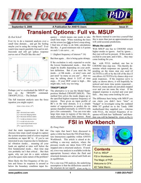
September 8, 2006 The Focus Issue 51 

September 8, 2006 A Publication for ANSYS Users Issue 51 

By Rod Scholl 

Transient Options: Full vs. MSUP 

Ever try to do a transient analysis over a 

small time domain… and get the feeling 

maybe you’re using the wrong tool? Ever 

watch time march painfully forward in milliseconds 

and still get spikey response 

curves out of /Post26 like this one? 

Perhaps you’ve overlooked the MSUP option 

on the TRNOPT command. 

TRNOPT,FULL – The Default 

The full transient analysis uses the force 

equation you might expect: 

And the main requirement is that one 

chooses time steps small enough to capture 

the system response (and of course required 

resolution on input BC’s). If you’re not 

interested in any response due to fundamental 

vibration modes… meaning all your 

loads are applied at rates well below the 

first fundamental mode… then time step 

size probably isn’t that critical… But then 

again, why not just do a static solution 

given the quasi-static nature of the problem? 

More likely the first frequency of the system 

and hence its response is around or 

below the boundary condition input frequency 

– which means one needs to take 

small time steps. When watching the lines 

on the screen (see link on how) creep along, 

I find lots of time to do little calculations 

like this. A good minimum rule is 8 points 

on each ½ sin curve… or: 

1 / (highest frequency of interest * 16) 

But then again… this is being quite skimpy. 

If the excitation is only expected to excite 

the lowest fundamental mode… then this 

might be doable depending on your problem 

definition. But if you need the 3rd 

mode… or 8th mode… or aren’t sure, and 

just need “as many as you can”… then we 

may be talking about A LOT of time 

steps… If your DOF count is high… this 

might take, well, way too long. 

TRNOPT,MSUP 

The alternative is to use the Modal Superposition 

Method (TRNOPT,MSUP). This 

method first solves the mode shapes up to 

the specified highest response frequency of 

interest. Then given an input profile of 

BC’s in the time domain, it is a simple 

matter of superposition to predict the response 

(handled internally in ANSYS with 

just a few commands). You can even take 

large time steps in regions of the time domain 

where you have little interest. Read 

By Doug Oatis 

the theory manual to convince yourself that 

this is more than just an approximation and 

will yield accurate predictions. 

Whats the catch? 

With MSUP one has to CHOOSE which 

higher modes to ignore. And by ignore… 

they just will not be present. If this mode is 

excited in your part, and it fails… they may 

come looking for you. 

But with FULL method, one has to 

CHOOSE time step size. This thereby determine 

which responses are ignored, depending 

on the times step size used (if 

AUTOTS is off) or by the roll of the dice if 

one allows AUTOTS to by chance skip over 

peak responses. If the response curve is 

spiky as shown above, it will hopefully be 

noticed and more time points requested… 

However, many peaks are just plain stepped 

over and you are none the wiser. If the 

skipped response is excited and your part 

fails… they may come looking for you. 

The difference here being with MSUP you 

can claim you didn’t have “time” or 

“budget” to investigate using the outdated 

8086 XT grafted on to the Tandy 1000 

motherboard they supplied you – whereas 

with FULL, the missed frequency of response 

will look less “deliberate” and therefore 

you will be burned by (Cont. on Pg. 2.) 

FSI in Workbench 

One topic that hasn’t been discussed in 

quite a while has been the FSI (Fluid-Structure 

Interaction) capability within ANSYS 

Workbench. This article is aimed at describing 

a one-way analysis, where the 

pressure results are taken from CFX and 

mapped onto a structural analysis. If needed, 

a two-way analysis is available (with the 

appropriate license) where the fluid and 

structural domains are solved until both are 

in equilibrium. 

For a one-way FSI analysis, the underlying 

assumption is that the deflections caused in 

the structure do not signifi- 

(Cont. on Pg. 3.) 

Contents 

Full vs. MSUP ................................1 

FSI in Workbench ...........................1 

The Magic of PGR ..........................3 

Welcome to CFX.............................4 

4D Table Macro...............................5 

www.padtinc.com 1 1-800-293-PADT


(Full vs. MSUP, Cont.) 

the angry mob of engineer non-believers. 

What’s the OTHER catch? 

Because the MSUP method requires a modal 

solution, the memory required for a given 

model is higher with MSUP than with the 

FULL method. I have found that if one has 

models this large, though, the FULL method 

is still prohibitive due to solve times for 

most common excitation pulses. And thus 

on today’s computers at least, speed and not 

memory is the limiting factor on solving 

transients with small time steps. 

An example -Try this one: Note the listed 

solve times. (I have to admit this script is 

adapted from one I found on my computer, 

and I don’t know who the original author 

was. So I thank you and apologize for not 

giving you credit.) Also, this wasn’t set up 

to skip a transient peak during a run – but 

that would be an even stronger demonstration 

for the value of the MSUP method. 

Below is a test case that attempts to capture 

the response of frequencies of the first five 

modes. 

In this last case, the number of time steps 

was chosen to yield a solve time of 1.8 hrs 

to be equal to the MSUP method tested 

above. You can see what kind of spikey 

response one gets for an equivalent solve 

time… 

You can download the files used at: 

ftp.padtinc.com/public/downloads/full_ms 

up.zip 

(FSI, Cont.) 

cantly impact the fluid domain. One example 

is the pressurization of an actuator cap, 

seen below. 

To begin, you must first create the fluid 

domain volume and mesh. Design Modeler 

is an excellent choice to do this with its Fill 

and Enclosure utilities. After the volume is 

created, you can use Simulation, CFX- 

Mesh, or ICEM-CFD to create the mesh. 

For the novice fluid mesher (of which I 

consider myself), Simulation or CFX-Mesh 

are the best choices. For the power-meshers 

out there, ICEM is your song. 

If you use CFX-Mesh or ICEM, you can 

create named selections/parts out of the 

surfaces that interface with the solid and 

pass them to CFX-Pre. For this example, I 

only looked at the stresses in the cap, so I 

made a named selection out of all the surfaces 

that match up with the cap. 

After you’ve solved the fluid domain, you 

can post-process as usual. Once you’re 

ready to solve the structural, you can reopen 

Design Modeler and prep the geometry 

for the structural analysis. For this example, 

I removed the pin-holes on the 

actuator cap, and suppressed out all bodies 

except for the cap. 

Once you bring the geometry into Simulation, 

go through your normal setup (i.e. 

define material properties, specify mesh 

controls, etc.). When you’re ready to load 

the part, simply apply a pressure to all the 

faces that match up to your fluid domain. In 

the details window for the pressure, change 

the ‘Constant’ to be ‘CFX Results’. You’ll 

then be prompted to select the result file 

(filename.res), region, and time step (if 

applicable). The regions will be listed for 

every surface that you have applied a 

boundary condition in CFX. For this example, 

I manually applied a wall BC to the FSI 

faces (even though all unconstrained faces 

have a wall applied to them). This enabled 

me to easily pick the region of the CFX 

model to pull the pressures from. 

After you specify the result file, region, and 

time step, Workbench will go off and interpolate 

the pressures onto the structural face. 

You’ll see 3 static isotropic pictures appear 

below the ‘Pressure’ in the tree. These will 

show the pressure values interpolated from 

the CFX model. After you solve the model, 

you’ll see an additional 3 pictures showing 

the pressures applied to the structural model. 

With a decent mesh, you should see the 

exact same pictures on both the CFX and 

Structural side. 

So now you’re probably thinking, “Well, 

that’s great, but what does this really do for 

me?” The short answer is that it allows you 

to better simulate your environment. Instead 

of assuming some sort of pressure 

distribution, you can use the actual gradient 

and better simulate reality. One thing you 

must always keep in mind, however, is to 




(FSI, Cont.) 

make sure you’re applying the proper pressure 

differential across the part. You need 

to make sure that the pressure calculated 

from CFX-Post represents absolute pressure. 

If not, you will need to pressurize the 

outer portion of your model to get the proper 

delta. 

The two-way FSI analysis is a bit more 

complicated, requiring ANSYS Classic 

knowledge in order to setup the Fluid and 

Structural interfaces (so each solver can 

pass info back and forth). The setup for this 

analysis should become easier in future 

releases as more ANSYS technologies are 

brought underneath the Workbench interface. 

Faster Results from Smaller 

Files: The Magic of PGR 

By Eric Miller 

Did you ever get frustrated by how long it 

sometimes takes to make a large and complex 

plot in ANSYS? Did you wonder why 

ANSYS has never done anything to speed 

up plotting and create smaller results files? 

Well guess what, they did do something 

years ago but most users don’t know it is 

there or have not made it a habit to use. The 

secret is the PGR file and a set of commands 

created to use it. 

Standard and Power Graphics 

Before delving in to the PGR file, it is a 

good idea to look at why the RST files that 

ANSYS makes are so big and why plots 

take so long. The answer is actually pretty 

simple and when you think about it, makes 

sense and like a lot of things falls under the 

old 80-20 rule. Approximately 80% (+/- 

15% or so depending on your actual needs) 

of the time users are plotting nodal result 

values on the external surface of their models. 

But, sometimes you need to have internal 

information, you want to do the nodal 

averaging differently, you want to look at 

results on a per-element basis, or you want 

to calculate the quality of your model by 

looking at the variation in results from element 

to element. For the 20% of the time 

you need to have the result that ANSYS 

calculated for each element at each node on 

the element. 

To understand this better think back to what 

happens in a solve. The program solves for 

the displacement of each node (DOF), then 

uses those values at each node in each element 

to calculate a stress and strain for that 

node and that element based upon the formulation 

and material properties of the element. 

ANSYS stores the results for each 

node in each element in the result file. A 

single nodal value for each node is not calculated 

until the user requests a plot. When 

this happens, the program must read the 

element based nodal results, average over 

each element that shares a given node, then 

store the resulting value in memory. 

So, the RST file is bigger than one would 

expect because each element stores results 

for each node on the element. If a node is 

shared by six elements, all the stress and 

strain information is stored six times! Also, 

all that data must be read into memory, 

sorted, averaged by node number, then plotted. 

That takes time and memory and is 

repeated for every plot. 

So to save memory and time, ANSYS introduced 

the PowerGraphics option many 

years ago. This changed the averaging algorithm 

to only look at nodes on the surface 

of an object when doing the averaging. This 

reduced the amount of memory required 

and speeds up the averaging calculation. It 

also, as most of you should have noticed by 

now, produces different results (search 

powergraphics at www.xansys.net). 

Solving the Time and File Issue 

After introducing Power- 


Advantages & 

Disadvantages of 

PowerGraphics? 

Even if you don’t use the PGR file, 

you can change the default plotting to 

or from PowerGraphics with the 

/GRAPHICS command. When using 

this option you can realize the following 

advantages: 

Faster plotting 

Curved element edges on quadratic 

elements 

Captures discontinuity from different 

materials 

Displays top and bottom stresses on 

shells at the same time 

Allows use of Query command to 

pick and see results on elements 

But there are some drawbacks: 

Does not work for circuit elements 

Averaging only uses elements with 

faces on the surface 

Min and Max values are for surface 

elements only 

No element coordinate system plotting 

To understand how stresses change, 

look at the example below. To get the 

stresses on the top surface: in full 

graphics, stress from the green and red 

dotted element corners are averaged. 

For PowerGraphics, only the green dotted 

ones are used. 



Graphics, the next logical step was to bypass 

the RST file and store the 

PowerGraphics information in a file during 

the solve. Now you have a much smaller 

file, your averaging is done only once, and 

you need a lot less memory. 

To use this file you simply need to 

tell ANSYS to create the PGR file 

during a solve, or if you forget 

about the command and want to do 

it after you have solved, you can 

generate a PGR file from a result 

file. The easiest way to do this is to 

use the GUI as shown in Figure 1. 

From the GUI you can see all the 

options that are available to you 

through the GUI or the PGWRITE 

command. Looking at these commands 

you can see that the PGR file 

offers a lot of control. 

First off, you can specify the filename. 

This way you can do things 

like create a separate file for each 

load step or, if you are using the command 

to extract key info from an existing RST 

file, you can create a PGR for each type of 

result data you want to store. 

This is often done by changing the settings 

on the next option, which controls the type 

of results to store. Since users usually only 

By: J Luis Rosales, PhD 

PADT has had the privilege of working 

with the world-class CFD program, CFX, 

for the past three years. During this time, 

we have solved small and simple models of 

a few thousand nodes to large and complex 

models with many millions of nodes. 

Before moving onto specific instruction, 

such as importing a mesh from another tool 

(a good topic for a future article) let’s start 

with a CFX overview. 

want stress results, choosing only that option 

can make the file much smaller. 

By default, the PGR file only uses average 

nodal values on the surface of your model. 

But if you need the internal information you 

can set it with the next option. You can also 

tell ANSYS to store unaveraged data, 

although doing so kind of destroys the 

point of using the PGR file. Lastly, 

you can tell the program to only store 

the internal information that is required 

for special plots like sections 

and vectors. This is a lot less data 

than the internal nodal information. 

Although it is much more efficient to 

create the file as part of the solution, 

you can always create it from an existing 

results file in POST1. When doing 

so you should be aware of a few 

things. First, you need to do a SET 

and a PGWRITE for each result set 

you want to store. Second, the results 

are stored in the current result coordinate 

system (RSYS). 

To use your PGR file you need to tell AN- 

SYS to not use the RST and point it to your 

smaller file with PGRPH,ON. Also, to get 

at different results sets, you simply use the 

PGRSET command instead of the SET 

command. And, if you want to look at a 

subset of nodes in the PGR file, use the 

PGSELE command. That is about it. 

How much Better is it? 

To get a feel for the difference, we dusted 

off our handy-dandy generic low pressure 

turbine disk and blade model (shown to the 

left as eye candy for the otherwise dull 

article) and did a static stress solution on it 

with PGWRITE turned on. Here are some 

statistics: 

Number of Nodes: 399,870 

Number of Elements: 268,507 

RST files size: 

PGR file size: 

Plot RST: 

ANSYS CFX: Welcome to CFX 

CFX is composed of three modules similar 

to the ANSYS architecture: CFX-Pre (a 

preprocessor), CFX-Solver (the solution 

solver) and CFX-Post (a post processor). 

These modules are started from a CFXlauncher 

window. CFX-Pre assumes you 

already have a meshed model and does not 

create the mesh. It is basically used to 

define the problem, apply boundary conditions 

and set up a few solver settings. 

CFX-Solver takes a *.def file created by 

CFX-Pre and solves the model to produce a 

solution. CFX-Solve can be as easy as 

clicking the solve button for a simple serial 

run to setting up a large distributed run for 

a multi-million node model. CFX-Post is 

easily one of the best post-processing tools 

that we have used for CFD results. The 

regular CFX tutorials do a very nice job of 

introducing users to the features available in 

CFX-Post; however, some information that 

may be of interest to users may be covered 

in future Focus articles. Also, CFX is a 

more advanced tool than the FLTORAN 

CFD code available in ANSYS. Flotran is 

of course still available. 

So pull out the CFX installation files, get a 

temp license from your ASD (if necessary) 

– and poke around the interface of this new 

member to the ANSYS family. 

615,120 MB 

50,790 MB 

8.3 msec 

Plot PGR: 

5.5 msec 

Faster, Smaller is Better 

The first thing that the data above points out 

is that computers have gotten so fast (we ran 

on a DUAL Opteron with 8GB of RAM) 

that the speed difference for a fairly normal 

model is small. But for larger models the 

difference becomes significant, and the files 

size change is significant. 

So, next time you start grumbling about 

shuffling around multi-gigabyte RST files, 

remember the lowly PGR file and give it a 

try. 



Awesome APDL: Writing a 4D Table to a File 

This month’s APDL macro is a nice example 

of how to write data from a four dimensional 

array to a text file. It was created 

because a customer needed to interpolate 

data based on X, Y, Z position and time. 

Once they made their table they wanted to 

store it in a text file for review. 

On first glance a simple task but it turns out 

that you need something special because the 

*MWRITE command only handles three 

dimensional arrays. So the solution is to 

write a 3D array for each of the fourth 

dimensions. 

This clever solution also shows how you 

can use the *cfwrite command to have a 

macro create a macro. This is how you can 

do text replacement on commands that 

don’t support it outwrite, like the *vwrite 

command. In this case, we use it so the 

name of the table can be a variable. 

Enjoy, and notice that we avoided the use of 

a tacky Twilight Zone joke... 

*dim,tabled,tab4,5,3,2,2 

! Loop on each dimension, 

! filling the table with some data 

*do,i,0,5 

*do,j,0,3 

*do,k,1,2 

*do,l,1,2 

tabled(i,j,k,l)=i+10*j+100*k+1000*l 

*enddo 

*enddo 

*enddo 

*enddo 

! Get a name from the user 

*ask,tab_name,Enter Table 

name,'tabled' 

!>>>> END OF PART1 

! Part 2 works on a table defined 

! by tab_name and can be 

! used in a generic way 

! 

! dimension size for 

*get,d_tabi,parm,%tab_name%,dim,x 

*get,d_tabj,parm,%tab_name%,dim,y 

*get,d_tabk,parm,%tab_name%,dim,z 

*get,d_tabl,parm,%tab_name%,dim,4 

k=1 

! Open a file to create the writing 

macro in 

*cfopen,dtable,mac 

! write out the command for 

! writing stuff 

*vwrite 

('*mwrite,%arg1%(0,0,k,l),d_test- 

%arg2%,txt') 

! Write out the format info 

*do,i,1,d_tabj+1 

*vwrite 

('%10.4F '$) 

*enddo 

! Done creating macro 

*cfclose 

!Loop on 4th dimension, calling 

! the macro you made 

*do,l,1,d_tabl 

dtable,tab_name,l 

*endd 

There have been lots of improvements to contact in recent years. Sheldon Imaoka shares a great 

PowerPoint that summarizes everything at: ansys.net/ansys/papers/nonlinear/contact_tech.pdf 

Ever thought about working for ANSYS, Inc? They have some nice jobs open right now. To see 

what is open, visit: ansys.recruitmax.com/candidates/default.cfm?szCategory=joblist 

Resources 

Upcoming Training Classes 

Month Start End # Title Location 

Sep ‘06 7-Sep 8-Sep 301 Heat Transfer Albq, NM 

11-Sep 13-Sep 101 Introduction to ANSYS, Part 1 Tempe, AZ 

18-Sep 21-Sep 802 Advanced APDL & Custom. Tempe, AZ 

25-Sep 26-Sep 201 Basic Structural Nonlinearities Tempe, AZ 

27-Sep 28-Sep 204 Adv. Contact and Bolt Pret. Tempe, AZ 

Oct ‘06 2-Oct 4-Oct 101 Introduction to ANSYS, Part 1 Albq. NM 

5-Oct 6-Oct 203 Dynamics Tempe, AZ 

9-Oct 10-Oct 100 Engineering with FE Analysis Irvine, CA 

16-Oct 18-Oct 104 ANSYS Workbench, Intro Albq, NM 

19-Oct 19-Oct 105 ANSYS Workbench, Struc NL Albq, NM 

25-Oct 27-Oct 902 Multiphysics for MEMS Tempe, AZ 

Nov ‘06 1-Nov 3-Nov 101 Introduction to ANSYS, Part 1 Tempe, AZ 

8-Nov 9-Nov 107 ANSYS WB DesignModeler Tempe, AZ 

13-Nov 14-Nov 301 Heat Transfer Irvine, CA 

16-Nov 17-Nov 102 Introduction to ANSYS, Part 2 Tempe, AZ 

27-Nov 28-Nov 604 Introduction to CFX Tempe, AZ 

Links 

News 

MatWeb now supports the creation of Workbench XML 

material files. Visit www.matweb.com to see PADT’s 

favorite on-line material repository 

Want to know which third party vendors are partnered 

with ANSYS, Inc? Visit 

www.ansys.com/corporate/partnerships.asp for a summary 

- China chooses ANSYS as standard in national 

engineering exam link 

- More Great Financial News: 

Highly Successful Second Quarter 

Name as Fortune Small Business Fastest 

Growing Companies for Third Consecutive 

Year link 

The Focus is a periodic publication of Phoenix Analysis & Design Technologies (PADT). 

Its goal is to educate and entertain the worldwide ANSYS user community. More information 

on this publication can be found at: http://www.padtinc.com/epubs/focus/about

Transient Options: Full vs. MSUP FSI in Workbench - PADT

Create successful ePaper yourself

Delete template?

Save as template?