The Ideal Profile AnalasisPhD Thesis by Thierry Worch

THESE/AGROCAMPUS OUEST
In Partnership with OP&P PRODUCT RESEARCH
To obtain the diploma of:
DOCTEUR DE L’INSTITUT SUPERIEUR DES SCIENCES AGRONOMIQUES, AGRO‐
LIMENTAIRES, HORTICOLES ET DU PAYSAGE
Specialization: Mathematic – Physics – Computer science
Doctorial school: Vie‐Agro‐Santé
Presented by:
Thierry WORCH
The Ideal Profile Analysis: From the validation to the statistical analysis of
Ideal Profile data.
Defended July the 9 th in front of the commission
Composition of the jury: Christopher FINDLAY President
Compusense Inc.
Marc DANZART
Reviewer
AgroParisTech, Massy
Halliday MACFIE
Reviewer
Hal MacFie Sensory Training Ltd
Jérôme PAGES
Advisor
Agrocampus Ouest, Rennes
Sébastien LE
Co‐advisor
Agrocampus Ouest, Rennes
Pieter PUNTER
Co‐advisor
OP&P Product Research, Utrecht
i

1
1 Illustration : Marion VIALADE
iii

Table of Contents
1. Introduction .................................................................................................................................. 11
2. The Ideal Profile Method in Practice. ........................................................................................... 19
2.1. Presentation of the Ideal Profile Method ............................................................................. 21
2.2. Complementary studies and justification of the point of views adopted ............................. 45
2.2.1. Correction of the ideal data .......................................................................................... 47
2.2.2. Justification of the correction ....................................................................................... 48
2.2.2.1. Relationship between perceived and ideal ratings ............................................... 48
2.2.2.2. Justification of the correction by translation ........................................................ 49
2.2.2.3. Should the ideal ratings be also standardized? ..................................................... 53
2.2.2.4. Conclusion ............................................................................................................. 56
2.2.3. Extension of the uniqueness of the ideal ratings at the consumer level ...................... 57
2.2.4. Extension of the typology of the consumers and attributes ......................................... 58
2.3. Conclusion ............................................................................................................................. 63
3. Consistency of the Ideal Profiles .................................................................................................. 67
3.1. Sensory Consistency of the Ideal Profiles .............................................................................. 71
3.1.1. Assessment of the consistency of the ideal profiles ..................................................... 73
3.1.2. Extension to L‐PLS, presentation of the methodology .................................................. 89
3.1.2.1. Algorithms ............................................................................................................. 90
3.1.2.2. Adaptations to our study ....................................................................................... 92
3.1.2.3. Results and discussion (perfume project) ............................................................. 93
3.1.2.4. Conclusions concerning the L‐PLS procedure........................................................ 96
3.1.3. Conclusions on the sensory consistency of the ideal data ............................................ 97
3.1.3.1. At the panel level ................................................................................................... 97
3.1.3.2. At the consumer level............................................................................................ 99
3.2. Hedonic Consistency of the Ideal Profiles ........................................................................... 101
3.2.1. Extension of the consistency of the ideal data ............................................................ 103
3.2.2. Complementary results on the simulations ................................................................ 113
3.2.2.1. Comparison of and ............................................................. 113
3.2.2.2. Error α in the selection of models ....................................................................... 118
3.2.3. General conclusions on the hedonic consistency of the ideal data ............................ 121
v

3.2.3.1. Quality of the individual models ......................................................................... 123
3.2.3.2. Significance of the liking potential ...................................................................... 125
3.2.3.3. (hedonic) consistency of the ideal profiles.......................................................... 126
4. The Ideal Profiles as a Tool for Optimization ............................................................................. 129
4.1. Pre‐Treatment of the Data .................................................................................................. 131
4.1.1. Clustering ..................................................................................................................... 133
4.1.2. Single vs. multiple ideals ............................................................................................. 137
4.2. The Ideal Product used as Reference .................................................................................. 149
4.2.1. Presentation of the IdMap .......................................................................................... 151
4.2.2. Complementary comparison between IdMap and PrefMapD .................................... 168
4.2.2.1. Level of acceptance in the PrefMapD ................................................................. 168
4.2.2.2. Stability of the PrefMapD .................................................................................... 172
4.3. Optimization Procedure using Ideal Profiles ....................................................................... 175
4.3.1. Review of the existing methodologies ........................................................................ 177
4.3.2. Proposition of a Product Based Optimization ............................................................. 178
5. General Conclusions: Validation of the IPA ............................................................................... 195
5.1. Description of the study ...................................................................................................... 197
5.1.1. The products ................................................................................................................ 197
5.1.2. The consumers ............................................................................................................ 197
5.1.3. Method ........................................................................................................................ 197
5.1.4. Preliminary study of the sensory space of the creams ............................................... 198
5.1.5. Preliminary study of the ideal product space.............................................................. 199
5.2. Consistency of the ideal data (§3.)...................................................................................... 201
5.2.1. Sensory consistency (§3.1) .......................................................................................... 201
5.2.2. Hedonic consistency (§3.2).......................................................................................... 203
5.3. Optimization of the tested products (§4.)........................................................................... 206
5.3.1. Segmentation of the panel and uniqueness of the ideal (§4.1).................................. 206
5.3.2. Determination of the sensory profile of the ideal product of reference (§4.2).......... 208
5.3.3. Optimization of the products according to the ideal of reference (§4.3)................... 210
5.4. Formulation of two new products ....................................................................................... 212
5.4.1. New sensory task ......................................................................................................... 212
5.4.2. Results: liking scores of the products .......................................................................... 213
vi

6. References................................................................................................................................... 217
7. Annexes ....................................................................................................................................... 223
7.1. Experts vs. Consumers ......................................................................................................... 225
7.2. Implementation in R ............................................................................................................ 239
7.2.1. The R‐Project and SensoMineR ................................................................................... 241
7.2.2. The Ideal Profile Analysis in R ...................................................................................... 241
7.2.2.1. Measuring the influence of the tested products on the ideal ratings ................ 241
7.2.2.2. Checking for multiple ideals ................................................................................ 242
7.2.2.3. Consistency of the ideal data .............................................................................. 242
7.2.2.4. Use of the ideal data ........................................................................................... 242
7.2.2.5. References ........................................................................................................... 243
Acknowledgements ............................................................................................................................ 245
vii

To all of you,
who are making my life
closer to Ideal.

1. Introduction

1. Introduction
For the Food and Cosmetics industry, optimization and innovation are important steps in product
development. This requires a good understanding of the products, both from a sensory point of view as well as
from a hedonic point of view. In other words, we need to understand how the products are perceived and how
the products are appreciated. Taken separately, this information is not sufficient for product improvement. But
combined, it is: we can determine which sensory characteristics drive the hedonic judgments. This relationship
is usually defined using statistical methods (Daillant‐Spinnler, MacFie, Beyts, & Hedderley, 1996). Once the
relationship between sensory characteristics and the hedonics is set, the industry can focus on these sensory
characteristics for product optimization (Moskowitz, 1995; Moskowitz, & Krieger, 1998).
First we need to gather the sensory and hedonic descriptions of the products. Current practice consists of
first asking subjects to describe the products according to a list of sensory attributes. This practice is known as
“descriptive analysis” (such as QDA®, Stone, Sidel, Woosley, & Singleton, 1974; Spectrum TM , Meilgaard, Civille,
& Carr, 2006) and results in “sensory profiles”. In descriptive analysis, subjects are asked to evaluate the
presented products in a monadic sequence and to rate the perceived intensity for each of them according to
the pre‐established list of sensory attributes. The products are presented one after the other according to a
pre‐established experimental design which takes care of order and carry over effects (MacFie, Bratchell,
Greenhoff, & Vallis, 1989). In general, the subjects who participate in these tests are either specialists who
know the family of products tested well, and hence are qualified as “experts” (e.g. oenologist tasting wine), or
people who are trained accordingly in order (1) to understand the sensory attributes used, (2) to detect the
differences between the products (discrimination of the products) and (3) to rate them adequately (consensus
between subjects) and repeatably (repeatability of the ratings) on the scale of notation used.
In parallel to the descriptive analysis to obtain the sensory profiles of the products, another test is
performed. During this test, subjects are asked to rate the same products on overall liking. In order to have
successful products, they must satisfy consumers. Hence, we need the judgments of the consumers about their
liking or acceptance of the products (i.e. consumers’ hedonic judgments).
After collecting the sensory and hedonic descriptions of the products they are linked in order to define
which sensory characteristics drive the hedonic judgments (Rivière, Monrozier, Rogeaux, Pagès, & Saporta,
2006). For this, we often use the preference mapping techniques (Carroll, 1972; Greenhoff, & MacFie, 1995;
Jaeger, Wakeling, & MacFie, 2000; Danzart, 2009a). In practice, two types of preference mapping techniques
exist: internal preference mapping (MDPref, Carroll, 1972) and external preference mapping (PrefMap, Carroll,
1972). A comparison of these two techniques is done by van Kleef, van Trijp, and Luning (2006).
Internal preference mapping starts with the hedonic ratings provided by the consumers, the sensory
profiles of the products being projected as supplementary variables in the hedonic space based on the linear
relationships between the hedonic data and the sensory attributes. External preference mapping starts with
the sensory description of the products. In this case, the hedonic scores provided by the consumers are
regressed in the sensory dimensions of product space on the sensory of the products. A common limitation in
sensory perception is related to the saturation of the sensory attributes. Indeed, the products which are not
sweet enough or on the other hand which are too sweet will not be fully appreciated. Hence, it is important to
consider this saturation effect within the individual models in order to define the optimal intensity of the
sensory attributes. To do so, quadratic effects as well as the interaction between the two first dimensions of
the sensory space are added to the linear effects (Danzart, 1998) within the individual models in the external
preference mapping. The individual models thus created are then applied to each point of the sensory space,
which allows defining a zone of acceptance for each consumer. These individual zones of acceptances are
13

1. Introduction
combined in order to define a global surface plot at the panel level. From this global surface plot we can define
the zone of the space in which the associated product would be accepted by a maximum of consumers (Mao, &
Danzart, 2008). The characteristics of this “ideal” product can then be defined and used as reference for the
optimization of the existing products, or for the formulation of a new potentially successful product (Danzart,
2009b; Moskowitz & Krieger, 1998; van Trijp, Punter, Mickartz, & Kruithof, 2007).
In order to get closer to the market, more importance should be given to the consumer. In this case, we
would prefer to use the sensory descriptions of the products obtained from consumers over the sensory
descriptions of the products obtained from experts or trained panelists. Thus, we would ask to the same
consumer to perform both tasks simultaneously, which results in sensory profiles and the hedonic judgments.
This procedure has the advantage that we can link the appreciation to the sensory perception of the products
directly for each consumer. This link hence seems more direct.
The "intensive" use of consumers for sensory tests is not accepted by everybody in the sensory
community. In the literature, numerous critics concerning the use of consumers for tests other then hedonic
have been formulated: (1) "…as with any untrained panel, beyond the overall acceptance judgment there is no
assurance that the responses are reliable or valid“ (Stone, & Sidel, 1993) and (2) “…consumers can only tell you
what they like or dislike” (Lawless, & Heymann, 1999). According to these authors, the use of consumers for
sensory descriptive tasks is not appropriate as consumers lack two major qualities: consensus and repeatability
to which we should add the uncertainty of the good comprehension of the meaning of the sensory attributes.
Moreover, Earthy, MacFie, and Hedderley (1997) showed that associating sensory questions with hedonic
questions can have an inconvenient halo effect. Although this effect is not always verified in practice (Popper,
Rosenstock, Schaidt, & Kroll, 2004), the long and thoughtful perception of the products can affect the hedonic
judgment of the consumers. This seems to be the price to pay if we wish to obtain sensory profiles from
consumers.
Other authors are more optimistic concerning the use of consumers to obtain sensory profiles. Moskowitz
(1996) and Husson, Le Dien, and Pagès (2001) have shown through different studies that consumers can
describe the sensory characteristics of the products with a precision comparable to the one obtained from
experts. In that case, the larger size of the consumer panel counterbalances the lack of training. On the other
hand, the use of consumers puts a restriction on the choice of sensory attributes used in the test. With
consumers, only “simple” sensory attributes can be used, we cannot use technical or chemical terms.
Since the use of consumers for descriptive tasks is highly important for the rest of this study, we had to
check the capacity of the consumers to provide valid sensory profiles of products. For that matter, we decided
to compare sensory profiles obtained from consumers with profiles obtained from experts for the same
products. This study is at the origin of the paper entitled “How reliable are the consumers? Comparison of
sensory profiles from consumers and experts” from Worch et al. presented in Annex (§7.1). In this example, we
have shown that the capacity of consumers in describing the sensory aspect of the products has the same
quality of discrimination and repeatability as that of experts.
Although the sensory and hedonic descriptions are obtained from the same consumers, we still need to
link them together. However, it can happen in some cases that the sensory descriptions and the hedonic
judgments are “independent”. This would correspond to the situation where the major sensory differences
which are detected do not influence the appreciation of the products for those consumers. In this case, the
user will not be able to find links between the hedonic and the sensory descriptions of the products (Faber,
14

1. Introduction
Mojet, & Poelman, 2003). This is the reason why integrating a reference to the hedonic within the description
of the products attribute by attribute has been considered. Such a task needs the use of consumers.
A first way of doing so consists in asking consumers to describe the perceived intensity of the products in
function of the representation they have of their ideal (Moskowitz, 1972; Shepherd, Smith, & Farleigh, 1989). In
this case, the consumers mention whether the product is too much, just about right or too little for each of the
attributes considered. The scale of notation thus used is known as JAR scale (Meullenet, Xiong, & Findlay, 2007;
Rothman, & Parker, 2009). In this case, the difference between the perceived intensity and the ideal intensity is
measured. However, the notion of “just about right” can be confusing. Indeed, for the consumers, does the jar
level refer to the acceptance of the product or to a preference (Gacula, Rutenbeck, Pollack, Resurreccion, &
Moskowitz, 2007)?
In the same purpose of integrating a reference to the hedonic in the description of the products attribute
by attribute, a second method consists in asking the consumers directly to describe their ideals, thus gathering
the hedonic and descriptive aspects of the products simultaneously (Moskowitz, 1972; Szcezsniak, Loew, &
Skinner, 1975). In practice, during such test, the consumers are asked to rate both the perceived and ideal
intensity of the products on a list of predefined attributes. In this case, the consumers are asked to rate their
ideal product on the same attributes and the same scale of notation as the tested products.
This technique, known as the Ideal Profile Method (IPM), is used by several professionals in industry.
Nevertheless, only few articles in the literature concerning the analysis of this particular data can be found.
Moreover, those articles only describe the testing protocol used and the final analysis of the data gathered.
From a practical point of view, these studies show that the use of ideal data brings useful information for the
optimization of products (Hoggan, 1975; Moskowitz, Stanley, & Chandler, 1977; Cooper, Earle, & Triggs, 1989).
However, the methodology of the IPM can be questioned. Indeed, the ideal profiles are fragile data since they
are provided by consumers who are describing fictive (ideal) products. So, which value can be granted to these
data? To which extent can the use of ideal profiles guide product optimization?
In order to answer these questions, we will have to get deeper insight in this data and thus try to better
understand how they are obtained.
This PhD document is first describing the Ideal Profile Method as it is used at OP&P Product Research. In
this case, the methodology consists in asking the consumers to describe their ideal for each product tested,
providing variability of ideal data between and within consumers. By studying the variability within consumers
we gain better insight in these data and can we study the impact of the tested product on the ideal.
Additionally, the study of the variability between consumers helps evaluating the degree of homogeneity at the
panel level.
In a second step, the value that can be granted to the ideal data is evaluated. To do so, a methodology to
measure the consistency of the ideal profiles has been set up. This methodology evaluates the link existing
between the sensory, hedonic and ideal descriptions by checking on the one hand whether the consumers
describe their ideal with similar sensory characteristics as the most appreciated product and on the other hand
whether the ideal product they defined is associated with a higher liking score than the tested products.
Once the consistency of the ideal data (as mentioned above) is checked, these data can be used to guide
on improvement. To do so, the principle of the external preference mapping technique adapted to our ideal
data is used. Hence, we have been adapting the treatment of the consumer data by integrating the variability
between and within consumers of the ideal data. This new procedure of optimization implies (1) the definition
of groups of consumers and homogeneous subcategories of products, (2) the choice of a consensual ideal
products used as reference to match in the optimization process (IdMap) and finally (3) the development of
15

1. Introduction
methodologies allowing the optimization of products based on the consensual ideal product defined previously
while taking into consideration the link between the perception of an attribute and the appreciation of the
products. To do so, the difference between the perceived and ideal intensity of each attribute is weighted
according to whether the attribute is a strong driver of liking or not.
The entire methodology developed through this PhD allows the complete analysis of the ideal data (from
checking for the consistency to the optimization of the products) and is referenced here as the Ideal Profile
Analysis (IPA).
The different parts of this thesis are articulated through one or many articles submitted or published in
Food Quality and Preference, to which are added “complement to the articles” presenting extensions or
justifications of the choices made for the methodology proposed.
Since The Ideal Profile Method has been applied for many years at OP&P Product Research, Utrecht, the
Netherlands, I had access to a large database. The methodologies developed in my PhD have been applied
systematically to a selection of 24 projects involving all types of food products (dairy products, candy bars,
soups, water, etc.). The choice of the projects has been based on the number of products involved (minimum
of 7 products) and of the experimental design used (only full designs). From these meta‐analyses were
extracted general tendencies related to the ideal descriptions. A list of the projects including the number of
products and consumers involved in the tests is presented Table 1.1.
project
#
products
#
consumers
#
attributes
project
#
products
#
consumers
#
attributes
Applesauce 8 180 23 Cream yoghurt 2 10 128 23
Beer 8 84 32 Ice cream 12 84 35
Croissants 9 151 26 Soup 1 9 109 25
Donuts 1 8 126 36 Soup 2 9 104 28
Donuts 2 8 167 28 Flavoured water 10 83 21
Licorice 9 80 22 Lemon water 9 100 23
Coffee 8 77 16 Candy bar 7 81 30
Meal salad 10 82 29 Vanilla dessert 8 76 30
Water 8 163 18 Milk drink 7 88 38
Perfume 14 103 21 Yoghurt 1 8 84 27
Rye bread 8 157 38 Yoghurt 2 9 117 29
Cream yoghurt 1 7 128 29 Organic yoghurt 8 127 34
Table 1.1: List of the 24 datasets considered for the meta‐analysis.
16

1. Introduction
Work accomplished
Articles
Articles accepted
Worch, T., Lê, S., Punter, P., & Pagès, J. (2013). Ideal Profile Method (IPM): the ins and outs. Food Quality and
Preference. In press (http://dx.doi.org/10.1016/j.foodqual.2012.08.001)
Worch, T., Lê, S., Punter, P., & Pagès, J. (2012). Construction of an Ideal Map (IdMap) based on the ideal
profiles obtained directly from consumers. Food Quality and Preference, 26, 93‐104.
Worch, T., Lê, S., Punter, P., & Pagès, J. (2012). Extension of the consistency of the data obtained with the Ideal
Profile Method: Would the ideal products be more liked than the tested products? Food Quality and
Preference, 26, 74‐80.
Worch, T., Lê, S., Punter, P., & Pagès, J. (2012). Assessment of the consistency of ideal profiles according to
non‐ideal data for IPM. Food Quality and Preference, 24, 99‐110.
Worch, T., Dooley, L., Meullenet, J.F., & Punter, P. (2010). Comparison of PLS dummy variables and Fishbone
method to determine optimal product characteristics from ideal profiles. Food Quality and Preference, 21,
1077‐1087.
Worch, T., Lê, S., & Punter, P. (2010). How reliable are the consumers? Comparison of sensory profiles from
consumers and experts. Food Quality and Preference, 21, 309‐318.
Jaeger, S.R., Bava, C.M., Worch, T., Dawson, J., & Marshall, D.D. (2011). The food choice kaleidoscope. A
framework for structured description of product, place and person as sources of variation in food choices.
Appetite, 56, 412‐423.
Articles submitted
Worch, T., & Ennis, J.M. Investigating the single ideal assumption using Ideal Profile Method. Submitted to Food
Quality and Preference.
Oral presentation (the name of the speaker is underlined)
Worch, T., Lê, S., Punter, P., & Pagès, J. Validation of the ideal profiles provided directly from consumers. 12 th
Agrostat Meeting, Paris, France.
Worch, T. The Ideal Profile Method. As part of the workshop: Current status and future directions for
alternative descriptive sensory methods workshop. 9 th Pangborn Meeting, Toronto, Canada.
Worch, T., Lê, S., & Pagès, J. Validation of the ideal data using Multivariate Analysis: the ideal products? Space
as a link between the products and their preferences. 50 th anniversary of CARME, Rennes, France.
Worch, T., Lê, S., Punter, P., & Pagès, J. Can the consumers express their needs? Use of Ideal Profiles to
understand and validate what is in the consumers’ mind. 2 nd Meeting of the Society of Sensory
Professional, Napa, USA.
Worch, T., Lê, S., Punter, P., & Pagès, J. What is in the consumer’s mind? Understanding and (external)
validation of Ideal Profile data. 4 th EuroSense conference, Vitoria‐Gasteiz, Spain.
Worch, T., Lê, S., Punter, P., & Pagès, J. Can we trust consumers’ ideal? Study of the relationship between the
consumers’ preference and their ideals. 10 th Sensometrics meeting, Rotterdam, the Netherlands.
17

1. Introduction
Punter, P., & Worch, T. The Ideal Profile Method: combining classical profiling with JAR methodology. 1st SPISE
meeting, HoChiMinh‐City, Vietnam.
Dooley, L., Worch, T., Meullenet, J.F., & Punter, P. Comparison of PLS and the Fishbone method to determine
optimal product characteristics. 8 th Pangborn Meeting, Firenze, Italy.
Worch, T., Lê, S., & Punter, P. How reliable are the consumers? Comparison of sensory profiles from consumers
and experts. 9 th Sensometrics meeting, St Catherines, Canada.
Worch, T., & Delcher, R. Evaluation of the panel and panelists performances in R. As part as the workshop on
Panel Performance, 9 th Sensometrics meeting, St Catherines, Canada.
Posters
Worch, T., Lê, S., Punter, P., & Pagès, J. Analyses of ideal data obtained by Ideal Profile Method to better
understand consumers and their needs. 9 th Pangborn Meeting, Toronto, Canada.
Worch, T., & Punter, P. Evaluation of the stability of the PCA products’ map in function of the data taken in
consideration. 10 th Agrostat Meeting, Louvain‐la‐Neuve, Belgium.
18

2. The Ideal Profile Method
in Practice.

2.1. Presentation of the
Ideal Profile Method

2. The Ideal Profile Method in Practice
In this section, the presentation of the Ideal Profile Method as well as a methodology developed for
understanding how consumers define their ideal is presented. This is done through the paper from Worch, Lê,
Punter, and Pagès (2013) entitled “The Ideal Profile Method (IPM): the ins and outs” published in Food Quality
and Preference, and completed with justifications of the correction and studies extending the analysis of the
variability between and within consumers of the ideal data. In this paper, the notations used for the rest of the
documents are presented.
As a reminder, the analyses developed along this document were applied to dataset from 24 different case
studies. More information concerning these studies is given in Table 1.1, page 16.
Journal:
Title:
Food Quality and Preference
Ideal Profile Method (IPM): the ins and outs.
Authors: Worch, T., Lê, S., Punter, P., & Pagès, J.
Abstract:
Keywords:
Reference:
The Ideal Profile Method is a sensory methodology mixing classical profiling (such as
QDA®) and JAR scale. It is performed by consumers who are asked to rate each product on
both their perceived and ideal intensities for a list of attributes. In the same test, consumers
also rate the products on liking.
The strength of such methodology is that it brings a lot of information about the products
and the consumers. Indeed each consumer provides the sensory profile of the products (i.e.
how do they perceive the products), their liking ratings (i.e. how do they appreciate the
products) as well as their ideal profiles (i.e. what are their expectations).
The ideal profiles are directly actionable to guide for products’ improvement. However,
this particular information should be carefully managed since it is obtained from consumers
and it describes virtual products. It relies on three main assumptions: (1) consumers should
rate a unique and stable ideal product, (2) consumers can describe different ideals and (3) the
ideal profiles provided by consumers should be consistent with the other descriptions (sensory
and hedonic).
The study of these assumptions on 24 projects help understanding the consumers and
how they define their ideals. It comes out that, although some consumers’ ideal ratings are
slightly influenced positively by the products, most of the consumers are reliable. Indeed, the
consumers rate unique ideal products which are consistent according to the sensory and
hedonic descriptions also provided. It also appears that it needs all to make a world, as
consumers show differences in their ideal products.
Consumer, ideal profiles, multiple ideals, descriptive analysis.
Worch, T., Lê, S., Punter, P., & Pagès, J. (2013). Ideal Profile Method (IPM): the ins and outs.
Food Quality and Preference, http://dx.doi.org/10.1016/j.foodqual.2012.08.001
23

2.1. Presentation of the Ideal Profile Method
1. Introduction
In sensory analysis, one of the main objectives is to characterize a set of products according to the way they are
perceived. To do so, a common practice consists in asking subjects to rate the products on the perceived intensities of a list
of attributes. This practice, also known as descriptive analysis (such as QDA®, Stone, Sidel, Oliver, Woolse, & Singleton,
1974), results in the definition of the sensory profile of the products, that is to say, a description of how these products are
perceived by the subjects. In fine, the objective of such methodology is to obtain a product space, which is a map
positioning the products that are perceived as similar close to each other, and placing apart those that are perceived as
different. For this task, the subjects considered are usually experts or trained panelists (i.e. subjects who have training
sessions during which they have learned to recognize and rate the perceived intensities of the pre‐established list of
attributes).
Although this methodology is extensively used, some alternative methods have been developed. These methods differ
according to the points of view adopted. Subjects can:
• be free in the choice of attributes used to describe the products in a sequential monadic way, as for example
in Free Choice Profiling (Williams, & Langrons, 1984) or Flash Profiling (Sieffermann, 2002; Dairou, &
Sieffermann, 2002);
• assess the entire product set simultaneously, as for example in Napping® (Pagès, 2005) or Ultra Flash Profile
(Perrin, Symoneaux, Master, Asselin, Jourjon, & Pagès, 2008);
• use holistic approaches to compare the products as in the case of Free Sorting Task (Lawless, 1989; Cadoret,
Lê, & Pagès, 2009), Hierarchical Sorting Task (Cadoret, Lê, & Pagès, 2011) or Sorted Napping (Pagès, Cadoret,
& Lê, 2010).
All these methodologies are defined as rapid methodologies because no or short training is required (Dehlholm,
Brockhoff, Meinert, Aaslyng, & Bredie, 2012). The different alternatives highlight different approaches, for example:
detailed vs. short description of the products, analytic vs. holistic approaches, use of trained panelists/experts vs. naïve
consumers (Gazano, Ballay, Eladan, & Sieffermann, 2005; Nestrud, & Lawless, 2008).
Due to the fact that consumers are being more and more involved in the product development process, their points of
view are currently often required. Moskowitz (1996), Husson, Le Dien, and Pagès (2001) and more recently Worch, Lê, and
Punter (2010) showed in different studies that consumers can profile products while meeting the requirements of
discrimination, consensus and reproducibility of a sensory panel. This is particularly true when the attributes which are
evaluated are not complex and understandable by naïve consumers.
It has also been shown that subjects can use an internal imagined product as reference to compare products (Booth,
Conner, & Marie, 1987). Such comparison is done when using tasks involving Just About Right (JAR) scales, in which
consumers are asked to rate the intensity of the products on each attribute by indicating whether the intensity of that
attribute is just about right, too strong, or too weak. The idea behind this is that if consumers can rate the perceived
intensities of the products in function of an imagined ideal that works as a reference, one can also expect them to be able
to rate their ideal explicitly.
Moskowitz (1972) worked on this idea and proposed to extend the classical sensory evaluation by integrating the
opinion of the subjects who test the food in the optimization process. To do so, he proposed to give the subjects the
opportunity to suggest the degree on a scale to which they would alter products for the given attribute set so that the
products would be closer to the representation of their ideals. Depending on the study, the subject was either asked to rate
the ideal directly (IPM type of measurement), or to rate the perceived intensity relatively to this ideal (JAR type of
measurement). Some years later, Szczesniak, Loew, and Skinner (1975) proposed a derivative of the texture profile
technique (Brandt, Skinner, & Coleman, 1963) using consumers. In their study, apart from providing descriptions of the
texture of the products, the consumers were also requested to rate the ideal intensity on the specific texture attributes.
Hoggan (1975) applied a similar technique for optimizing beers, by including taste attributes as well. In these two studies,
the ideal intensity was rated only once by each consumer.
The Ideal Profile Method (IPM), which is presented in this paper, is a variant of these methodologies. After presenting
in detail the protocol as used routinely at OP&P Product Research (Utrecht, The Netherlands), guidelines for a better
understanding of how consumers define and rate their ideals towards a product are given.
2. The Ideal Profile Method, in practice
The Ideal Profile Method (IPM) is a descriptive analysis performed by consumers where additional questions about the
ideal intensities and liking are asked. In practice, each consumer assesses a series of products, and rates each product on
the same set of sensory attributes. The products are presented in randomized monadic sequence in order to avoid firstorder
and carry‐over effects (MacFie, Bratchell, Greenhoff, & Vallis, 1989). For each attribute, both the perceived and ideal
intensities are rated on the same type of scale (here, an unstructured scale with unique unlabeled anchors at 10% and 90%
is used). So, if the first question is: "Please rate the sweetness of this product", the second question will be: "Please rate
your ideal sweetness for this product". This methodology has been adopted with the aim to mimic the JAR scale, but using
the perceived and ideal intensities instead of the difference with an imagined ideal.
24

2. The Ideal Profile Method in Practice
At the end of the task, each consumer has rated as many times the profile of his/her "ideal product" (also called ideal
profile) as he/she has tested products using the same set of attributes. Thus, if a consumer rates the profiles of P products,
he/she also rates P times his/her ideal profile. As mentioned earlier, also hedonic questions are asked for each product
using a 9‐point category scale, after the sensory and ideal ratings. So summarizing, at the end of the test, each consumer
has provided information about his/her sensory and hedonic appraisal of the products as well as the description of his/her
ideal product (Figure 1).
Figure 1: Data provided by each consumer during the IPM.
Unlike experts or trained panelists, consumers do not take part in any prior training. For this reason, the size of the
panel must be larger: in practice the authors use a panel size of around 100 consumers, which is considered to be a reliable
number of participants in this kind of tasks (Moskowitz, 1997).
Another option of this methodology would be to ask the consumers to rate their ideal profiles only once. In this latter
case, each consumer would rate P+1 profiles vs. 2*P as in the methodology described above. Since Szczesniak et al. (1975)
concluded that it makes little difference in the results whether the ideal product is described before or after tasting the set
of samples, the ideal intensities could be rated either at the end of test, after the consumers have tasted and rated all the
products, or at the beginning, before consumers have even started tasting the products. As this perspective has not been
tested by the authors yet, no comparative information concerning the outcomes can be given.
3. Material and method
3.1. Material
To illustrate the statistical methodology for a better understanding of the ideal profiles provided by consumers, 24
datasets obtained with the IPM are used. A summary of the 24 datasets is given in Table 2.
project # of products # of consumers project # of products # of consumers
Applesauce 8 180 Cream yoghurt 2 10 128
Beer 8 84 Ice cream 12 84
Croissant 9 151 Soup 1 9 109
Donuts 1 8 126 Soup 2 9 104
Donuts 2 8 167 Flavoured water 10 83
Licorice 9 80 Lemon water 9 100
Coffee 8 77 Candy bar 7 81
Meal salad 10 82 Vanilla dessert 8 76
Water 8 163 Milk drink 7 88
Perfume 14 103 Yoghurt 1 8 84
Rye bread 8 157 Yoghurt 2 9 117
Cream yoghurt 1 7 128 Organic yoghurt 8 127
Table 2: List of the dataset considered.
As all the datasets were obtained in a similar way, only one of them (the perfume dataset, Worch et al., 2010) will be
described in detail here. It concerned 12 luxurious women perfumes (Table 3) rated on 21 attributes (listed in Table 3) by
103 Dutch consumers in two 1‐hour sessions.
25

2.1. Presentation of the Ideal Profile Method
Products Type Attributes
Angel Eau de Parfum Intensity Spicy
Cinema Eau de Parfum Freshness Woody
Pleasures Eau de Parfum Jasmine Leather
Aromatics Elixir Eau de Parfum Rose Nutty
Lolita Lempicka Eau de Parfum Chamomile Musk
Chanel N⁰5 Eau de Parfum Fresh lemon Animal
L’Instant Eau de Parfum Vanilla Earthy
J’Adore (EP) Eau de Parfum Citrus Incense
J’Adore (ET) Eau de Toilette Anis Green
Pure Poison Eau de Parfum Sweet fruit
Shalimar Eau de Toilette Honey
Coco Mademoiselle Eau de Parfum Caramel
Table 3: List of products and attributes.
Note: during the test, the products Pure Poison and Shalimar were duplicated.
Further in the document, particular results from two other studies are presented. These results are obtained from (1) a
case study on croissants involving 151 consumers who rated 9 products on both perceived and ideal intensity for 26
attributes, and (2) a yoghurt study (cream yoghurt 1) involving 128 Dutch consumers who rated 7 products on 29 attributes.
In both cases, the products were also rated on overall liking.
3.2. Notation
Let P denote the number of products tested, A the number of attributes used to describe the products and J the
number of consumers who participated in the test. The following notation will be used to describe the data obtained from
IPM (vectors are in bold):
: intensity perceived by the consumer j for the product p and the attribute a;
. ; 1: : vector of intensities perceived by the consumer j for the P products and the attribute a;
. : average over the index p; average intensity perceived by the consumer j on attribute a over the P products (Table
1a);
.
Consumer j Attribute 1 … Attribute a … Attribute A
Product 1
…
Product p
…
Product P
.
Table 1a: Organization and notation of the sensory data provided by each consumer.
: ideal intensity of the attribute a provided by the consumer j after testing the product p;
. ; 1: : vector of ideal intensities of the attribute a provided by the consumer j for the P products;
.: average over the index p; average ideal intensity of the attribute a provided by the consumer j over the P products
(Table 1b);
.
Consumer j Attribute 1 … Attribute a … Attribute A
Product 1
…
Product p
…
Product P
.
Table 1b: Organization and notation of the ideal data provided by each consumer.
26

2. The Ideal Profile Method in Practice
: hedonic judgment provided by the consumer j for the product p;
. ; 1: : vector of hedonic judgments provided by the consumer j for the P products.
As mentioned in the previous section, in the studies performed, consumers rated as many times their ideal profile as
they test products. If the set of samples preferably belong to the same category and type, normally people would rate their
ideal attributes of the products tested in a consistent way (all of them being very similar, if not the same. Each consumer
will be assigned a unique ideal profile which corresponds to the averaged ideal rating he/she gave for each attribute. This
averaged ideal profile is denoted .. .; 1: and is defined by (Eq.1):
. ∑
.. . ; 1:
(1)
Since consumers do not use the scale in the same way, it is important to correct their averaged ideal profiles before
comparing them. The correction for the use of the scale is done by translating the consumers’ averaged ideal profile
according to the averaged perceived intensities they also provided. It is done by subtracting the averaged perceived
intensities over the P products for each consumer and each attribute from his averaged ideal profile (Eq.2). This ideal profile
corrected is noted .. .
̃. . . (2)
.. ̃. ; 1:
Additional explanations concerning this correction are given in the Appendix.
3.3. Method
The aim of gathering ideal information from consumers is to optimize products. Since companies cannot create an
optimized product for each single consumer, a solution that would satisfy a maximum number of consumers should be
considered. For that matter, most of the optimization procedures found in the literature (Szczesniak et al., 1975; Hoggan,
1975; Cooper, Earle, & Triggs, 1989) use the averaged ideal product for the entire panel of consumers as a reference to
match. Although this averaged ideal product is not the optimal product for all the consumers (in practice, it is often
observed that a small proportion of consumers appreciate more the least liked products of the majority), it has been shown
it would be a satisfying solution (Hoggan, 1975).
Still, one can be interested in the differences between consumers in their ideal profiles. For such analysis, considering
the averaged ideal profile for each consumer is often required. Since consumers rate their ideal for each product tested,
one should check first whether the consumers rate repeatedly a unique ideal or if the ideals for each tested products are
different. This could be the case for products which are very different from a sensory point of view.
Two questions arise: At the panel level, do all the consumers share a common ideal product, or do consumers differ in
their definition of the ideal product? At the consumer level, do consumers have (and rate) a single ideal, or do they rate
multiple ideals?
To answer these questions, the variability of the ideal ratings is studied. This variability will be analyzed in three
different ways:
• the variability of the ideal ratings according to the tested products;
• the variability of the ideal ratings within consumers;
• the variability of the ideal ratings between consumers.
The study of the variability of the ideal ratings at these different levels helps concluding whether the consumers
describe one or multiple ideals. It can be check both at the panel (based on all attributes or for each attribute separately)
and consumer level.
3.3.1. Do consumers rate one or multiple ideals?
In practice, it is common to test products with similar sensory characteristics and similar usage. In this case, one would
say that the products tested should belong to the same “category” (e.g. soda drinks, cookies, dairy products, etc.).
However, depending on the purpose of the test, the products tested can vary slightly (e.g., natural crisps from different
brands, which, it could be said, belong to the same subcategory of product) or largely (e.g., using coke drinks, orange soda
drinks, or iced teas, in a soda test, which would belong to different subcategories).
The optimization procedure often assumes that consumers would associate the products tested to one unique ideal
product. This assumption seems fair for products with very similar sensory characteristics; However, it shows limits when
products are more different (the sensory characteristics of an ideal orange soda drink do not necessarily match the sensory
characteristics of the ideal coke drink for a same consumer). In the latter case, it could happen that consumers have
multiple ideals, one for each subgroup (or subcategory) of products. The different subcategories of products can be defined
according to different sensory characteristics, which can either be due to the recipes solely (e.g., coke vs. orange flavored
27

2.1. Presentation of the Ideal Profile Method
types of soda), or to the context of usage too (e.g., perfume for the day or for the night). In that case, it is important to
optimize each product according the ideal product of its corresponding subcategory.
In practice, defining subcategories of products is very subjective. Some consumers might consider a group of products
as from the same subcategory (and hence will associate them to one unique ideal) while some others would not (and hence
will provide multiple ideals). By considering that each subcategory of product is associated to one unique ideal, we will
propose a methodology (single vs. multiple ideal) which allows checking for subcategories of products within the product
set tested using the ideal information provided by the consumers. Since we are not interested in differences within
consumers here, the procedure proposed is performed at the panel level.
3.3.1.1. Panel level:
Since the optimization procedure is performed at the panel level, one should look for global patterns in the ideal
ratings, to see whether or not the panel (as a whole) is influenced by the tested products. In the case the panel rates one
unique ideal product, the averaged ideal product can be used to optimize all the products. In the contrary, if the panel rates
multiple ideals, the optimization of the different subsets of products should be done according to the adequate ideal
product.
To check for these patterns, an averaged ideal product is calculated over the consumers based on the product in
question: P tested products yield P averaged ideal products. Then, the uniqueness of the ideal descriptions is checked
through the closeness of the profile of the P averaged ideal products. This can be done globally (i.e. based on all attributes)
or for each attribute separately.
When all the attributes are considered together, the uniqueness of the ideal products can be evaluated through the
distance between the projections of the P averaged ideal products into the sensory product space. To do so, the sensory
product space is created by PCA on the sensory profiles of the tested products. The P averaged ideal products are then
projected as supplementary products into that space. If the projections of the different ideal products are close in the
sensory space, consumers rate one unique ideal. In the contrary, if the projections of the P ideal products define clear
different groups on the space, consumers describe multiple ideals.
Since the notion of distance between the projections is subjective, this procedure is enriched by considering the
variability existing around each ideal product via confidence ellipses (Husson, Lê, & Pagès, 2005). These confidence ellipses
are obtained using partial bootstrap (Cadoret, & Husson, 2012): It consists in simulating fictitious panels by resampling
randomly with replacement the original one, and by projecting the averaged ideal profiles (called simulated ideals) obtained
from the simulated panels into the same sensory space. This procedure is iterated a large number of times (in practice 500
times) and confidence ellipses containing 95% of the projections of the corresponding simulated ideals are constructed
around each product.
Inspecting the resulting maps, it could be said that the panel of consumers has rated a unique ideal if the projections of
the ideal products are close in the sensory space, involving an overlap of the confidence ellipses. On the contrary, they have
rated multiple ideals if the projections of the ideal products are far on the space. In this latter situation, the corresponding
confidence ellipses do not overlap. Since observing an overlap of the ellipses is not sufficient to conclude about the
significant differences between ideal products (the differences could be observed on other sensory dimensions of the PCA),
this procedure is completed by the Hotelling T² test. This MANOVA helps defining whether the ideals are significantly
different or not, hence helping to define the number of subcategories of products to consider in the mind of the consumers.
The uniqueness of the ideal descriptions can also be evaluated for each attribute separately. To do so, a two‐way
ANOVA, which measures the product and consumer effects on each ideal attribute, is performed (Eq. 3a).
Where
is the constant, γ pa the product effect, β ja the consumer effect (random) and ε jpa the residual
In this ANOVA, the uniqueness of the ideal ratings for an attribute a is measured through the product effect . One
has to consider the particular case where the product effect is significant. In that situation, the ideal and perceived
intensities are compared to determine whether the differences in the ideal ratings are due to the existence of multiple
ideals or just an artifact due to the sensory differences of the tested products on that attribute. To do so, the value
associated with the product effect in Eq.3a is compared to the corresponding value of the product effect measured for
the perceived intensities on the corresponding attribute (Eq. 3b).
(3b)
Where
is the constant, γ pa the product effect, β ja the consumer effect (random) and ε jpa the residual
To facilitate the interpretation of the result, the ratio is considered. This ratio is considered since and
are comparable values measuring the part of variability related to the products on respectively the perceived and ideal
intensity, and made relative according to the residual of the respective models. In this case, we are directly interested in the
one‐to‐one comparison of the F values. For that reason, the ratio is considered and compared to the value 1. When
consumers rate multiple ideals, a large ratio (close or larger than 1) is expected.
28
(3a)

2. The Ideal Profile Method in Practice
Additionally, for those ideal attributes with a significant product effect, the influence of the tested products on the
ideal ratings is evaluated. To do so, the P coefficients associated with the different products are extracted for each
attribute from Eq. 3a. The link between these coefficients and the sensory descriptions of the products is measured (Table
4) using the correlation coefficient between the perception of the products on an attribute a and the impact of the
products on the ideal ratings of that attribute a. If the correlation coefficient is positive (vs. negative), the consumers rate
their ideals as more intense (vs. less intense) for the attribute a after rating a product perceived as more intense on the
same attribute a. A dragging (vs. compensating) effect is then observed.
Product
Perc.
attr. 1
…
Perc.
attr. a
…
Perc.
attr. A
Influence
on attr. 1
…
Influence
on attr. a
…
Influence
on attr. A
1
…
p .
…
P (active) (supplementary)
Table 4: Organization of the perceived intensities (left)
and of the influence of the products on the ideal ratings (right) submitted to the PCA.
To view simultaneously this relationship for all attributes, a PCA is performed on the averaged table of perceived
intensities, where the influence of the product on the ideal ratings is projected as illustrative variables.
3.3.1.2. Consumer level:
The uniqueness of the ideal ratings on the different attributes can also be evaluated at the consumer level. Let’s
consider that each consumer rates one unique ideal on each attribute. This ideal rating can be defined by Eq. 4a.
where equals the corrected ideal intensity of the consumer j for the attribute a and the residual.
(4a)
The uniqueness of the ideal rating is measured within the residual .
Specifically, when the P ideal ratings provided
by a consumer are close, indicating a low variability of the ideal ratings, the sum of squares of the residual is small.
Inversely, a consumer providing different ideal ratings is associated with a large sum of squares of the residual. The value
per se of the sum of squares does not give any conclusion. Therefore it is compared to the corresponding sum of squares of
the residual obtained from the perceived intensities provided by the same consumer. In other words, the residual is
compared with the residual
obtained from Eq. 4b:
where the averaged perceived intensity of the attribute a by the consumer j and
the residual
(4b)
To facilitate the comparison, the ratio
between the sums of squares is used. For consumers
having one unique ideal product, this ratio is expected to be lower than 1.
3.3.2. How do consumers differ in their representation of their ideal?
For the optimization process, the averaged ideal product for the entire panel is often considered as a reference to
match. But does this averaged ideal product correspond to an optimum product to all consumers? Do they all share a close
ideal?
To answer this question, the focus is on the variability of the averaged ideal profiles provided from each consumer (i.e.
the variability between consumers’ ideals). To evaluate such differences, one might be interested in creating an ideal space
where consumers sharing similar ideals are grouped together and apart from those who have different ideals. Such ideal
space can be obtained by PCA on the corrected averaged ideal profiles (a justification of the use of the corrected averaged
ideal profiles is given in the Appendix). In this analysis, each entity corresponds to the corrected averaged ideal profile ..
provided by a consumer.
The ideal space allows creating a typology of consumers which can be enriched by associating each homogeneous
group of consumers with the closest‐to‐their‐ideal tested product. To do so, the sensory profiles of the products are
projected as illustrative entities in this space (Table 5).
29

2.1. Presentation of the Ideal Profile Method
consumer 1
Attribute 1 … Attribute a … Attribute A
…
consumer j ̃.
…
consumer J
(active)
product 1
…
product p . ..
…
product P
(supplementary)
Table 5: Organization of the ideal profiles used for the construction of the ideal space,
with projection of the products as supplementary.
4. Results
4.1. Single vs. multiple ideals
The uniqueness of the ideal representations has been checked both at the panel and consumer level. At the panel
level, it is checked globally (based on all attributes) and for each attribute separately.
4.1.1. At the panel level
4.1.1.1. Globally
For the croissant project, the projections of the averaged ideal products for the panel are all located in a close area of
the map, in the bottom right corner of the sensory space (Figure 2). Since the confidence ellipses constructed around the
ideal products all overlap, it could be concluded that at the panel level, consumers are rating one single ideal. However, this
conclusion is to relativize since the first two dimensions only explain around 55% of the total variance, and important
differences might also be seen on higher dimensions. But since all the p‐values associated to the Hotelling T² test are not
significant (see Table 6) in this particular project, the optimization of all the products can be done based on one unique
ideal which would be the averaged over all these individual ideals.
Figure 2: 95% confidence ellipses associated to the averaged ideal products of the panel for the croissant project.
30

2. The Ideal Profile Method in Practice
1 2 3 4 5 6 7 8 9
1 1,000 0,687 0,206 0,530 0,907 0,492 0,337 0,784 0,986
2 0,687 1,000 0,564 0,795 0,759 0,325 0,235 0,278 0,602
3 0,206 0,564 1,000 0,795 0,375 0,038 0,026 0,055 0,151
4 0,530 0,795 0,795 1,000 0,768 0,122 0,080 0,227 0,439
5 0,907 0,759 0,375 0,768 1,000 0,289 0,186 0,606 0,838
6 0,492 0,325 0,038 0,122 0,289 1,000 0,948 0,415 0,590
7 0,337 0,235 0,026 0,080 0,186 0,948 1,000 0,276 0,421
8 0,784 0,278 0,055 0,227 0,606 0,415 0,276 1,000 0,819
9 0,986 0,602 0,151 0,439 0,838 0,590 0,421 0,819 1,000
Table 6: P‐values obtained with the Hotelling T² test showing the significant differences between each pair of products for
the croissant study.
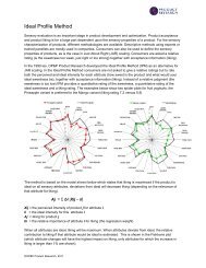
Figure 3a shows the results obtained for the cream yoghurt 1 project. In this dataset, it can be seen that the
confidence ellipses associated to the ideal product 7 is different from the other ideals. Indeed, the confidence ellipse of the
ideal product 7 is not overlapping the confidence ellipses associated to the other ideal products. This separation is observed
on the second dimension. Hence it involves different ideal intensities (Figure 3b) for the attributes fresh taste, sour odour,
fruity taste (stronger ideal intensity for 7) and sweet taste, sweet odour, amount fruit (weaker ideal intensity for 7). This
result is confirmed by the p‐value obtained with the Hotelling T² test given in Table 7. A closer look at this table also shows
a significant difference between the product 3 and the five other products. Indeed, the confidence ellipse associated to the
product 3 does not overlap with the other ellipses on the second dimension. In this case, it would also be recommended to
optimize the product 3 separately. However, since the difference between the ideal product associated to 3 and the ideal
product common to the five other products would be small, for this project, it would be recommended to optimize the
product 7 based on its corresponding ideal, and to optimize the six other products together based on their common ideal.
Figure 3a: 95% confidence ellipses associated to the averaged ideal products of the panel for the cream yoghurt 1 project.
31

2.1. Presentation of the Ideal Profile Method
Figure 3b: Correlation circle associated to the product space obtained for the cream yoghurt 1 project.
1 2 3 4 5 6 7
1 1,000 0,402 0,032 0,184 0,628 0,498 0,000
2 0,402 1,000 0,005 0,813 0,851 0,431 0,000
3 0,032 0,005 1,000 0,006 0,027 0,001 0,000
4 0,184 0,813 0,006 1,000 0,601 0,157 0,000
5 0,628 0,851 0,027 0,601 1,000 0,333 0,000
6 0,498 0,431 0,001 0,157 0,333 1,000 0,000
7 0,000 0,000 0,000 0,000 0,000 0,000 1,000
Table 7: P‐values obtained with the Hotelling T² test showing the significant differences between each pair of products for
the cream yoghurt 1 study.
4.1.1.2. For each attribute
At the attribute level, the definition of a single ideal was done by comparing the ratio of F values associated to the
product effect on the different perceived and ideal intensities. Figure 4 shows the ratio across attributes for the different
projects. As can be seen, most of the ratios are smaller than 1, meaning that the consumers described one unique ideal for
the majority of the attributes. However, for some projects, such as the beer or candy bar projects, ratios larger than 1 are
observed. For these attributes (length of the after taste, bitter taste and musty taste for the beers; saltiness and crunchiness
for the candy bar) of these products, consumers seemed to rate multiple ideals.
32

2. The Ideal Profile Method in Practice
Figure 4: Distribution of the ratio of the F of the product effects for the perceived and ideal intensities in each project.
4.1.1.3. Influence of the products on the ideal ratings
In order to check whether the ideal ratings are independent from the products tested, a two‐way ANOVA measuring
the product and consumer effects on each ideal attribute was performed. In this ANOVA, we are only interested in the
product effect which is expected not to be significant. However, this is not always true. For some consumers and attributes,
the product effect is significant. It is the case for 13 out of 21 attributes in the perfume example. To check the nature of this
product effect, the individual coefficients were extracted from this ANOVA (Eq. 3a) and were associated with the
perceived intensities (Table 4). A PCA was performed on the product profiles and the coefficients were projected as
supplementary variables in this analysis.
Figure 5 shows that the correlation between pairs of corresponding attributes is always strong and positive. When
products were perceived as more intense, consumers tended to rate their ideal as more intense. This phenomenon can be
defined as a dragging effect of the perceived intensities on the ideal ratings observed for each attribute. This dragging
effect was observed in all datasets.
Figure 5 Relationship between the perceived intensities and the influence of the products on the ideal ratings for the
perfume dataset (significant level for the attributes: ***

2.1. Presentation of the Ideal Profile Method
The next step was to measure the impact of this dragging effect. To do so, the averaged ideal ratings . were
compared to the averaged perceived intensities . , and the magnitude of the influence of the products on the ideal
ratings was measured.
The simultaneous representation of the averaged perceived intensities and the averaged ideal ratings (Figure 6) allows
quantifying the dragging effect. For the perfume dataset, no impact is observed for the attribute intensity (Figure 6a),
although the products are different. However, for freshness (Figure 6b), a dragging effect is observed: the fresher the
product, the higher the ideal freshness. But although the products are clearly different in freshness, the ideal ratings only
vary a little. It seems here that consumers rated one unique ideal for freshness.
Figure 6: Influence of the perceived intensities (boxplot) on the ideal ratings (dotted line) for a non significant (intensity, a)
and a significant (freshness, b) attribute.
4.1.2. At the consumer level
To check for uniqueness of the ideal, the ratio
was considered (Eq. 4).
When consumers rate unique ideals, the variability of the ideal ratings is low compared to the one associated with the
products. For all the dataset considered, the majority of the ratios were lower than 1 (Figure 7), the median being often
lower than 0.5. Given that the variability of the ideal ratings was much smaller than the variability of the perceived
intensities, it can be concluded that for the majority of consumers, one unique ideal was found.
Figure 7: Ratio of the sum of squares of the residual obtained with each project.
Note: for graphical reasons, all ratio larger than 2 is forced at 2.
34

2. The Ideal Profile Method in Practice
This corresponds for example to the consumer 12535 (perfume dataset) for whom both perceived and ideal intensities
are represented Figure 8a. This is what one can expect from consumers (i.e. consumers providing close ideal ratings which
are independent of the product tested). In some rare occasions, the ratio might take larger values, showing that consumers
might describe multiple ideals. For consumer 13313, the ratio was close to 1 (Figure 8b) which means that he/she rated the
ideal with the same variability as the products. For some other consumers, this ratio was even larger. A closer inspection at
the ideal descriptions seems to show that they had difficulties describing their ideals. For consumer 13645 (Figure 9a), the
high ratio is due to a non‐discrimination of the products and not to a description of different ideals. For consumer 13121
(Figure 9b), the high ratio seem to be due to some difficulties in understanding or rating the products on some attributes.
Indeed, this consumer rated both the perceived and ideal intensities identical (using only values between 15 and 20 on a
100‐point scale) for the entire set of attributes (with the exception of freshness and intensity).
Figure 8: Raw perceived and ideal intensities provided by two particular consumers (perfume dataset): (a): the consumer is
associated to a ratio 1 ; (b): the consumer has a ratio ~1.
35

2.1. Presentation of the Ideal Profile Method
4.2. Variability of the averaged ideal profiles
In order to study the variability between consumers’ ideals, a PCA was performed on the corrected averaged ideal
profiles. To characterize groups of consumers sharing a similar ideal, the tested products were projected as supplementary
entities into the resulting space.
Since consumers were corrected for their different use of the scale, the first dimension of the PCA obtained with the
perfume dataset opposes consumers (i.e. 2909) who described their ideals as less intense for all attributes to consumers
(i.e. 13645) who described their ideals as more intense for all attributes (Figure 10). As the projection of the products as
supplementary entities are not well separated on the first dimension, the dimensions 2 and 3 were considered for further
interpretation (Figure 11). Here, the ideal space opposes the consumers 11169 and 12872 on the 2 nd dimension (Figure
11a). This corresponds to consumers describing their ideals respectively with strong oriental notes vs. consumers describing
their ideals with strong fresh and fruity notes (Figure 11b). The projection of the products as supplementary entities
associated ideal products described with strong oriental notes (i.e. consumer 1169) with the products Shalimar, Angel and
Aromatic Elixir. Ideal products with strong fresh and fruity notes were associated with the products J'Adore, Coco
Mademoiselle and Pleasures (i.e. consumer 3670). The 3rd dimension shows the particular case of the consumers describing
their ideals with strong honey, caramel and vanilla notes. These consumers (i.e. consumer 13311) have ideals whose
profiles are close to those of Lolita Lempicka and Cinema.
Figure 10a: Ideal space (dimensions 1 and 2) with projection of the products as supplementary entities.
Figure 10b: Variables representation associated with the ideal space (dimensions 1 and 2).
36

2. The Ideal Profile Method in Practice
Figure 11a: Ideal space (dimensions 2 and 3) with projection of the products as supplementary entities.
Figure 11b: Variables representation associated with the ideal space (dimensions 2 and 3).
Although all consumers did not share the same ideal, it was possible to define groups of consumers sharing similar
ideals. These groups could then be characterized by the products via their proximity in the space. However, some
consumers were located far away from these groups, their ideal ratings being more extreme (Figure 11a). For these
particular consumers, the characteristics of their ideal products were similar to the ones of the products, but required much
stronger intensities.
This remark can be seen as a limitation of the IPM. Indeed, for some attributes (more precisely the ones with hedonic
connotations such as freshness for mint gum, natural taste for fruit juice or throat burn for chocolate), the ideal level will
never be achieved as consumers will always ask for more (or less). This is why the ideal ratings provided by consumers
should be used as guidance to an improvement and not as a strict recipe. Moreover, in the process of optimizing products,
it is important to consider both the deviation between the perceived and the ideal intensity for each product and each
attribute, and the impact of that attribute on liking. Some methods for optimization which take these two parameters into
consideration are given in Worch, Dooley, Meullenet, and Punter (2010). The methods presented in this article provide
some estimation of the drop in liking score for each product for not being ideal.
37

2.1. Presentation of the Ideal Profile Method
4.3. Summary
To summarize the results obtained previously, one can model the ideal ratings provided by the consumers. When
consumers rated one unique ideal, the simple model used to characterize the ideal rating was presented (Eq. 4a). When
consumers rated multiple ideals (based on all attributes), the same procedure can be applied to each subset of products
associated with a unique ideal. The corresponding model obtained at the panel level is given Eq. 5:
(5)
However, the study of the relationship between the ideal and perceived intensities showed that the ideal ratings could
be influenced by the perceived intensities of the products. The model can be extended by considering this influence. The
direct relationship between the perceived intensity and the ideal rating is considered and a regression factor is added (Eq.
6):
(6)
with the slope of the regression line of the perceived on the ideal intensity provided by the consumer j for the
attribute a.
It has also been shown that it takes all kinds to make a world. Consumers do not necessarily share a common ideal.
Hence, it is important to include the differences between consumers in the model. Not being interested in these consumers
specifically, the consumer effect is set as random. The following model of analysis of covariance is obtained (Eq. 7):
where is the consumer effect set as random.
(7)
The diversity of consumers was not only measured through the direct differences between their ideals (measured by
the consumer effect) but also through the different influence of the products on the ideal ratings. While rating the ideal
intensity of an attribute a, some consumers might have been positively influenced by the products while others might have
been influenced negatively or not at all. The interaction between the influence of the perceived intensities on the ideal
ratings and the consumer is added to the previous model (Eq. 8):
: (8)
In this analysis of covariance, the interaction : measures the influence of the products on the ideal ratings
for each consumer.
With this model, the ideal information as well as the impact of the different factors on the ideal ratings (tested
products, differences between consumers) can be estimated at once for each attribute. This can only be done if the ideal
ratings have been rated multiple times by each consumer. A more detailed study of the coefficients of this ANCOVA can
help to better understand the ideal ratings.
5. Conclusions
The IPM is a sensory evaluation methodology combining classical profiling with ideal ratings measured from
consumers. It provides additional information (ideal profiles) which can be useful for product optimization (Worch et al.,
2010). However, the IPM provides more detailed information than JAR scales (Van Trijp, Punter, Mickartz, & Kruithof, 2007)
as both the perceived and ideal intensities for each attribute are measured, while only deviations from ideals are measured
with JAR scales. This is why many practitioners have applied methods measuring ideal information in the past 40 years.
Due to the diversity of the data acquired with IPM, Worch, Lê, Punter, and Pagès (2012a, 2012b) proposed a
methodology which checks the sensory and hedonic consistency of the ideal information. This consistency is checked by
evaluating the agreement between the different types of data (sensory, hedonic, and ideal). In practice, consistent ideal
ratings could be considered to be efficient since they validate all types of data at once. However, in practice, those cases
where the three data sets are not in agreement would normally be interpreted as an inconsistency of the ideal ratings,
since it is hard to imagine consumers providing good ideal ratings on one hand, and hedonic judgments which are not
related to the sensory descriptions on the other hand. However, it has to be said that these apparently “inconsistent” ideal
ratings can be really consistent if it happens to be that consumers rate their ideals according to other criteria than liking.
For example, consumers on a diet, could like more those sweeter products, but would give a consistent ideal product which
is low in sweetness, since they have health concerns. Such cases have not been taken into consideration here, but would be
highly suggested.
In this context, one should be cautious when improving the products. Such verification of the consistency of the
dataset is not possible with other methodologies such as the JAR scale since all the information (sensory, ideal, and
hedonic) is needed. However, for these methodologies, other validations (e.g. significance testing) based on bootstrap
techniques could be performed.
38

2. The Ideal Profile Method in Practice
With the IPM, the ideal information provided from consumers is directly actionable for product optimization. In order
to avoid any misuse of this information, it is important to understand how consumers define their ideal. Some clues can be
given by the study of the variability of the ideal ratings at both the panel and consumer level, as well as between and within
consumers.
From our experience, in most cases, consumers associated the product set to one unique ideal when based on all
attributes. However, when attributes are considered separately, multiple ideals could be observed for some of them. At the
consumer level, some show large variability in their ideal ratings. This is either due to 1) difficulties with rating their ideal
intensities, 2) difficulties with the task, or 3) because they consider the products tested coming from different
subcategories.
When projects include products belonging to one unique subcategory, it could be interesting to ask the ideal only once
to consumers. By doing so, the methodology is simplified for the consumers. However, since it has been shown that
consumers were influenced by the products tested while rating their ideal intensities, it might be preferable to ask for their
ideal intensities prior to the products evaluation. Since the consumers cannot use a tested product as a reference to
describe his/her ideal product anymore, using a structured labeled scale for the entire task would be helpful in that
situation.
In the optimization process based on ideal products measured directly from consumers, the averaged ideal product
calculated over the panel is often considered. By doing so, one supposes that consumers share close ideal profiles. This
hypothesis was checked in a second step by studying the variability of the averaged ideal ratings between consumers. From
this analysis, it was shown that consumers differ in their conception of their ideals, highlighting that “it takes all kinds to
make a world”. Hence considering one averaged ideal for the entire panel as a reference to match in the optimization
process might not lead to an optimal solution. Other ideal solutions might satisfy the consumers more: Among them, we
can mention the solution obtained with the Ideal Mapping technique (IdMap, Worch, Lê, Punter, & Pagès, 2012c) which
consists in taking the averaged ideal profile common to a maximum of consumers only. In this latter, the ideal product is
more targeted since it is optimal for the larger subgroup of consumers sharing a common ideal.
In summary, we consider that IPM is a valuable methodology for products’ optimization.
Appendix
For the evaluation of the variability of the ideal profiles between consumers, a map is created positioning the
consumers together based on the proximity of their ideal products. Such ideal space has been obtained by performing a
PCA on so‐called corrected averaged ideal profiles .. . These profiles correspond to the averaged ideal profiles of the
consumers after correcting for the difference in use of the scale. Hence, the data considered for each consumer is the
difference ̃. between his/her averaged ideal score . and his/her averaged perceived score of the products . .
By doing so, all consumers are translated by setting their averaged perceived intensity at the same origin, and the
differences between consumers only concern the ideal profiles they provided. For a consumer j, a positive (vs. negative)
difference ̃. means the ideal is described as more (vs. less) intense than the averaged perceived intensity of the tested
product.
In order to check whether the correction is relevant, the same methodology for studying the variability of the ideal
products between consumers is performed on the non‐corrected data. A PCA is performed on the averaged ideal profiles ..
directly. Since the dimensions of the PCA are not interpreted, the variable names are hidden.
In order to check whether the consumers’ differences in their use of the scale has an impact on the results, the
averaged perceived intensities . from each consumer are projected as illustrative variable on this PCA (Table A1).
Ideal att. 1 … Ideal att. a … Ideal att. A Perc. att. 1 … Perc. att. a … Perc. att. A
Cons. 1
…
Cons. j . .
…
Cons. J (active) (illustrative)
Table A1: Organization of the data used to justify the correction of the ideal profiles.
In this case, the PCA is performed on the averaged ideal profiles .. and the averaged perceived intensities .. are projected
as illustrative variables.
It is considered here that, if a consumer j 1 uses a higher part of the scale than a consumer j 2 to describe the products,
then j 1 will also use a higher part of the scale than j 2 to describe the same ideal. When the ideal data are not corrected from
the use of the scale, the PCA might separate these consumers while they should belong to the same group, as they share
the same ideal.
In the case where the ideal space opposes consumers according to differences in the use of the scales, the projection
of the averaged perceived intensities . would be highly positively correlated to the averaged ideal attributes ..
Otherwise, the projections would be orthogonal.
39

2.1. Presentation of the Ideal Profile Method
The PCA performed on the non‐corrected ideal profiles returns the following results (Figure A1). The correlation circle
(Figure A1b) shows that the first dimension is strongly positively correlated with all the attributes. This particular situation ‐
also known as size effect‐ explains 54% of the variance. It opposes consumers who scored their ideal low on all attributes
(i.e. 4238) to consumers who scored all attributes high (i.e. 8118) (Figure A1a). This difference between consumers can
either be related to their ideal (some want an ideal which is not intense for all attributes while some other look for an ideal
that is more intense on all attributes), or to the scaling behavior of the consumers themselves (some using only the low part
of the scale while some use only the high part of the scale).
Figure A1: First and second dimensions of the ideal space obtained with the non‐corrected averaged ideal profiles.
To conclude about the nature of the differences between consumers, the averaged perceived intensities . are
projected as illustrative (Figure A2).
Figure A2: Projection of the averaged perceived intensities as illustrative variables in the ideal space.
The consumers’ averaged perceived intensities for each attribute are also projected along the first dimension and are
highly positively correlated with the corresponding ideal attributes. In other words, a similar size effect is observed with the
perceived intensities, meaning that consumers who rated the products using the higher (vs. lower) part of the scale tended
to use the scale in the same manner when rating their ideal intensities. This is observed for all attributes. Hence, the
differences between consumers highlighted by the first dimension of the PCA are related to a different use of the scale and
not to their ideals.
40

2. The Ideal Profile Method in Practice
Since the differences in the use of the scale are an important part of the variability, it is important to correct it. Hence,
using the corrected averaged ideal profiles instead of the non‐corrected averaged ideal profiles seems relevant. However,
one has to be sure that the ideal data are corrected for the differences in the use of the scale.
To check that, the consumers’ differences (i.e. the averaged perceived intensities . ) are also projected on the ideal
space obtained from the corrected averaged ideal profiles .. (Table A2).
Ideal att. 1 … Ideal att. a … Ideal att. A Perc. att. 1 … Perc. att. a … Perc. att. A
Cons. 1
…
Cons. j ̃. .
…
Cons. J (active) (illustrative)
Table A2: Organization of the data used to justify the correction of the ideal profiles.
In this case, the PCA is performed on the corrected averaged ideal profiles .. and the averaged perceived intensities .. are
projected as illustrative variables.
The PCA performed on the corrected averaged ideal profiles, in which the averaged perceived intensities per consumer
are projected as illustrative (Table A2), highlights another size effect on the first dimension (Figure A3). Indeed, all the
corrected ideal attributes are once again highly positively correlated with the first dimension.
Figure A3: Projection of the averaged perceived intensities in the ideal space obtained from the corrected averaged ideal
profiles.
The projections as illustrative variables of the averaged perceived intensities are orthogonal to the corrected ideal
attributes. The ideal data are corrected from the differences in the use of the scale. The size effect highlighted here on the
first dimension is related to differences in the consumers’ ideals, meaning that some consumers (i.e. 2909) described their
ideal as less intense than what they perceived for all attributes while for some others (i.e. 13645), the ideal should be more
intense on all attributes than what they perceived. Further interpretation of this ideal space is given in the article.
As a conclusion, the correction of the ideal data from the consumers’ differences in the use of the scale is done by
translating their ideal ratings according to their averaged perceived intensity.
Acknowledgement
The authors would like to thank the reviewers for their valuable comments which helped improving considerably this
manuscript, as well as Prof. Danzart and Betina Piqueras for their valuable input related to the topics covered in this paper.
41

2.1. Presentation of the Ideal Profile Method
References
Booth, D.A., Conner, M.T., & Marie, S. (1987). Sweetness
and food selection: measurement of sweetners’
effects on acceptance. In Sweetness (ed. J.
Dobbing), Springer‐Verlag: London.
Brandt, M.S., Skinner, E.Z., & Coleman, J.A. (1963).
Texture profile method. Journal of Food Science,
28: 404.
Cadoret, M., & Husson, F. (2012). Confidence ellipses in
holistic approaches. Oral presentation in 12 th
European Symposium on Statistical Methods for
the Food Industry, Feb.‐March, Paris, France.
Cadoret, M., Lê, S., & Pagès, J. (2009). A Factorial
Approach for Sorting Task data (FAST). Food
Quality and Preference, 20, 410‐417.
Cadoret, M., Lê, S., & Pagès, J. (2011). Statistical analysis
of hierarchical sorting data. Journal of Sensory
Studies, 26, 96‐105.
Cooper, H.R., Earle, M.D., & Triggs, C.M. (1989). Ratios of
Ideals – A New Twist to an Old Idea. In Product
Testing with Consumers for Research Guidance.
ASTM STP 1035, L.S. Wu, Ed., American Society for
Testing and Materials, Philadelphia, 54‐63.
Dairou, V., & Sieffermann, J.M. (2002). A comparison of
14 jams characterized by conventional profile and
a quick original method, the Flash Profile. Journal
of Food Science, 67, 2, 826‐834.
Dehlholm, C., Brockhoff, P.B., Meinert, L., Aaslyng, M.D.,
& Bredie, W.L.P. (2012). Rapid Descriptive Sensory
Methods: Comparison of Free Multiple Sorting,
Partial Napping, Napping, Flash Profiling and
Conventional Profiling. Food Quality and
Preference, 26, 267‐277.
Gazano, G., Ballay, S., Eladan, N., & Siefferman, J.M.
(2005). Flash profile and flagrance research: Using
the words of the naïve consumers to better grasp
the perfume’s universe. In ESOMAR fragrance
research conference, 15‐17 May 2005, New York,
USA.
Hoggan, J. (1975). New Product Development. MBAA
Technical Quarterly, 12, 81‐86.
Husson, F., Le Dien, S., & Pagès, J. (2001). Which value
can be granted to sensory profiles given by
consumers? Methodology and results. Food
Quality and Preference, 12, 291‐296.
Husson, F., Lê, S., & Pagès, J. (2005). Confidence ellipse
for the sensory profiles obtained by principal
component analysis. Food Quality and preference,
16, 245‐250.
Lawless, H.T. (1989). Exploration of fragrance categories
and ambiguous odors using multidimensional
scaling and cluster analysis. Chemical Senses, 14,
349‐360.
MacFie, H.J., Bratchell, N., Greenhoff, K., & Vallis, L.V.
(1989). Designs to balance the effect of order of
presentation and first‐order carry‐over effects in
hall tests. Journal of Sensory Studies, 4, 129‐148.
Moskowitz, H.R. (1972). Subjective ideals and sensory
optimization in evaluating perceptual dimensions
in food. Journal of Applied Psychology, 56, 60‐66.
Moskowitz, H.R. (1996). Experts versus consumers: A
comparison. Journal of Sensory Studies, 11, 19‐37.
Moskowitz, H.R. (1997). Base size in product testing: a
psychophysical viewpoint and analysis. Food
Quality and Preference, 8, 247‐255.
Nestrud, M.A., & Lawless, H.T. (2008). Perceptual
mapping of citrus juices using projective mapping
and profiling data from culinary professionals and
consumers. Food Quality and Preference, 19, 431‐
438.
Pagès, J. (2005). Collection and analysis of perceived
product inter‐distances using multiple factor
analysis: Application to the study of 10 white wines
from the Loire Valley. Food Quality and Preference,
16, 642‐649.
Pagès, J., Cadoret, M., & Lê, S. (2010). The Sorted
Napping: a new holistic approach in sensory
evaluation. Journal of Sensory Studies, 25, 637‐658.
Perrin, L., Symoneaux, R., Maître, I., Asselin, C., Jourjon,
F., & Pagès, J. (2008). Comparison of three sensory
methods for use with the Napping® procedure:
Case of ten wines from Loire Valley. Food Quality
and Preference, 19, 1‐11.
Sieffermann, J.M. (2002). Flash profiling. A new method
of sensory descriptive analysis. In AIFST 35 th
convention, July 21‐24, Sidney, Australia.
Stone, H., Sidel, J., Oliver, S., Woosley, A., & Singleton,
R.C. (1974). Sensory evaluation by quantitative
descriptive analysis. Food Technology, 28, 24‐34.
Szczesniak, A.S., Loew, B.L., & Skinner, E.Z. (1975).
Consumer texture profile technique. Journal of
Food Science, 40, 1253‐1256.
Van Trijp, H.C.M., Punter, P.H., Mickartz, F., & Kruithof,
L. (2007). The quest for the ideal product:
Comparing different methods and approaches.
Food Quality and Preference, 18, 729‐740.
42

2. The Ideal Profile Method in Practice
Williams, A.A., & Langron, S.P. (1984). The use of freechoice
profiling for the evaluation of commercial
ports. Journal of the Science of Food and
Agriculture, 35, 558‐568.
Worch, T., Dooley, L., Meullenet, J.F., & Punter, P.H.
(2010). Comparison of PLS dummy variables and
Fishbone method to determine optimal product
characteristics from ideal profiles. Food Quality
and Preference, 21, 1077‐1087.
Worch, T., Lê, S., & Punter, P.H. (2010). How reliable are
the consumers? Comparison of sensory profiles
from consumers and experts. Food Quality and
Preference, 21, 309‐318.
Worch, T., Lê, S., Punter, P.H., & Pagès, J. (2012a).
Assessment of the consistency of the ideal profiles
according to non‐ideal data for IPM. Food Quality
and Preference, 24, 99‐110.
Worch, T., Lê, S., Punter, P.H., & Pagès, J. (2012b).
Extension of the consistency of the data obtained
with the Ideal Profile Method: Would the ideal
products be more liked than the tested products?
Food Quality and Preference, 26, 74‐80.
Worch, T., Lê, S., Punter, P., & Pagès, J. (2012c).
Construction of an Ideal Map (IdMap) based on the
ideal profiles obtained directly from consumers.
Food Quality and Preference, 26, 93‐104.
43

2.2. Complementary studies and
justification of the point of views adopted

2. The Ideal Profile Method in Practice
In this paper, it has been shown that the ideal information provided by consumers can be noised by
consumers’ variability due to differences in the use of the scale. Instead of using the raw ideal data, the
difference between ideal and perceived intensity is considered. This difference (also called correction) is
defined and justified here. Moreover, to understand the consumers’ ideals, the variability of the ideal ratings
was studied between and within consumers. An extension of this analysis is also presented here.
2.2.1. Correction of the ideal data
In order to "correct" the ideal profiles from the differences in the use of the scale, a transformation of the
ideal data was proposed in the article §2.1. However, other corrections could be considered. Rather than
considering the raw ideal intensities as provided by each consumer, they can be made relative to the
perceived intensities also provided by the same consumer as proposed in Figure 2.1:
1.
2.
3.
4.
5.
y jpa
y j.a z jpa z j.a
Figure 2.1: Different possible correction of the ideal data.
Attribute a
1:
The difference between the ideal intensity of the attribute a (provided by the consumer j for the product
p) and the perceived intensity of the attribute a (provided by the consumer j for the product p). This approach
is interesting for the optimization of the products at the consumers’ level (JAR scale inverse).
2: . .
The difference between the ideal and the perceived intensities of the attribute a after averaging over the P
products for the consumer j. This difference represents the ideal intensity for the attribute a of the averaged
ideal product provided by the consumer j, after homogenizing from the different use of the scale. This
approach is the one adopted and this corrected ideal intensity is denoted (Eq.2.1a):
̃. . .
(2.1a)
with
.. ̃. ; 1: : vector of ideal intensities averaged over the index p and corrected according to the
averaged intensities perceived by the consumer j considered for the A attributes. This vector is also called
“corrected averaged ideal profile of the consumer j”.
This correction consists in a translation of the ideal information according to the perceived intensity. An
additional step consisting in standardizing this difference can be performed. In that case, the quantity ̃. is
47

Complementary Studies
divided by the standard deviation .
of the perceived intensities provided by the consumer j for the attribute
a (Eq. 2.1b).
standardized ̃. z .
σ .
(2.1b)
For the rest of the document, the translated version of the ideal intensity ̃. is preferred over its
standardized version.
3: .
The difference between the intensity of the attribute a perceived by the consumer j for the product p and
the averaged ideal intensity of the same attribute a provided by the consumer j. This approach is interesting for
the optimization on an individual basis of the products taken separately based on the averaged ideal products.
It is very similar to the first difference presented above.
4: .
The difference between the ideal intensity of the attribute a provided by the consumer j after testing the
product p and the averaged perceived intensity for that attribute a by the consumer j. This difference
corresponds to the corrected ideal intensity of the attribute a provided by the consumer j after testing the
product p. This correction is interesting to study the variability between consumers from all the individual ideal
profiles they provide.
5: .
The difference between the ideal intensity of the attribute a provided by the consumer j after testing the
product p and the ideal intensity averaged over the P products for the same consumer j and the same attribute
a. Here, the transformation is similar to centering the ideal profiles of a consumer. This difference is useful to
measure the variability within each consumer of the ideal profiles he/she provided.
The correction by translating the ideal information according to the averaged perceived intensity is similar
to JAR scale except that in JAR situation, the anchor point used to homogenize the consumers is their ideal. The
consumers rate the products on a list of attributes by indicating whether the perceived intensity is just about
right (the perceived intensity equals the ideal intensity), too little (the perceived intensity is lower than ideal) or
too much (the perceived intensity is higher than ideal).
But is this correction necessary and relevant? After investigating the relationship between the perceived
and ideal intensity ratings provided by each consumer, the advantage of such correction is evaluated at both
the panel and consumer level. Additional analyses comparing results obtained from translated and
standardized ideal intensity are also given.
2.2.2. Justification of the correction
2.2.2.1. Relationship between perceived and ideal ratings
In the article, it was shown that the consumers are influenced by the products tested while rating their
ideals. When a product is perceived as strong for an attribute, the ideal rating of that attribute is also rated
stronger. This result suggests the existence of a relationship between these two ratings. To test this, the
relationship between the perceived and ideal ratings provided by the same consumer was measured. As only
48

2. The Ideal Profile Method in Practice
linear relationships are expected, the correlation coefficient . ; . was computed for each consumer
between the vectors of perceived and ideal intensity for each attribute.
The correlation coefficient was calculated for each consumer and each attribute separately for the 24
different projects. The distribution of these correlation coefficients for each project is given in Figure 2.2
Figure 2.2: Distribution of the correlation coefficients between perceived and ideal intensities
for each consumers and each attribute per project.
In all the projects, the distribution of the correlation coefficients shows a strong linear relationship
between the perceived and ideal ratings. In most cases, the median is larger than 0.5. The perceived and ideal
ratings provided by each consumer are dependent. The larger the perceived intensity rating for a product, the
larger the corresponding ideal rating. This corresponds to the dragging effect presented in the article.
In sensory analysis, it is also known that consumers don’t use the response scale the same way. Since the
ideal ratings and the perceived intensity ratings are correlated, one can expect that the ideal ratings are also
noised by the differences in the consumers’ use of the scale. As this variability is less relevant, it is important to
correct it. This is why a simple but essential correction was proposed in the article. This correction is justified
here both at the panel and consumer level.
2.2.2.2. Justification of the correction by translation
2.2.2.2.1. Justification at the panel level
The importance of correcting the ideal data from the differences in the use of the scale was justified at the
panel level in the Appendix of the article presented in §2.1. This justification was done based on the study of
the variability of the ideal profiles between consumers.
This justification can be extended at the consumers’ level.
49

Complementary Studies
2.2.2.2.2. Justification at the consumers’ level
At the consumers’ level, the justification of the correction of the ideal data is done through an indicator.
The indicator used here is the correlation coefficient ,,
measuring the sensory consistency of the ideal
profiles provided by each consumer. More details about this coefficient are given in the article assessing the
sensory consistency of the ideal profiles (see §3.1.1).
For each consumer, the vector of linear drivers of liking/disliking was calculated using the correlation
coefficient between the vector of perceived intensity for each attribute . and the vector of liking ratings . .
This vector of linear drivers of liking/disliking was compared to the ideal ratings given by the corresponding
consumer j. Again, the correlation coefficient was used. In the article §3.1.1, only the corrected ideal ratings
were considered (Eq. 2.2a). Let’s compare it to the results obtained with the non‐corrected ideal ratings (Eq.
2.2b).
,,
. ; . ; .
. . ,,
The distributions of the correlation coefficients ,,
. ; . ; .
and . . ,,
obtained from the corrected and noncorrected
ideal ratings are compared graphically in Figure 2.3 for the perfume dataset.
(2.2a)
(2.2b)
Figure 2.3: Truncated distribution of the ,,
and . . ,,
obtained with the corrected and non‐corrected ideal ratings.
Note: The distributions reach values larger than 1. This is an artifact due to the estimation of the distribution, the
correlation coefficients being comprised between ‐1 and 1.
The truncated distributions show higher coefficients when the ideal ratings are corrected. In other words,
correcting for the differences in the use of the scales removes noise due to irrelevant variability which results in
higher sensory consistency. This can be explained by the fact that using the difference between the ideal and
the perceived intensity of an attribute gives information about the direction to change. This direction should be
in agreement with the nature of the attribute (i.e. driver of liking or disliking). For drivers of liking (vs. disliking),
the more (vs. the less) the better, so the difference between the ideal and perceived intensity should be
positive (vs. negative). When the ideal data are not corrected, the correlation reflects the intensity ratings
between attributes. In that case, the stronger (vs. weaker) drivers of liking should also be the attribute
associated with the higher (vs. lower) ideal intensity. This is not necessarily true in practice.
50

2. The Ideal Profile Method in Practice
Additionally, the one to one comparison of ,,
the consumers are associated with a ,,
and . . ,,
(Figure 2.4) shows that although most of
coefficient which is higher than the . . ,,
(i.e. consumers
located above the bisection line), it is not always the case. Indeed, in few cases (i.e. 11169), using the non‐
corrected ideal ratings returns a higher coefficient. Still the paired t‐test performed between the ,,
. . ,,
coefficients shows significant differences (Table 2.1).
Mean difference
(corrected‐non corrected)
t‐value df p‐value
t‐test 0.18 4.95 102

Complementary Studies
Figure 2.5: ,,
and . . ,,
coefficients obtained with the corrected (left) and non‐corrected (right)
ideal ratings for the different projects.
The paired t‐test (Table 2.2) performed between the two series of coefficients show significant difference
in favor of ,,
for 15 out of the 24 projects. Still for one project, significant differences were found in favor of
. . ,,
(croissant project). For the 8 remaining projects, no significant differences between the two series of
coefficients were observed. In most of the cases, using the corrected ideal ratings lead to higher correlations.
52

2. The Ideal Profile Method in Practice
Mean difference
(cor.‐non cor.)
t‐value df p‐value
Mean difference
(cor.‐non cor.)
t‐value df p‐value
Applesauce 0.01 0.78 177 0.44 Cream yoghurt2 ‐0.02 ‐0.78 127 0.44
Beer 0.15 6.87 81

Complementary Studies
Figure 2.6: PCA performed on the standardized averaged ideal products
In Figure 2.6, the first dimension is the particular case of the consumer 13645. A closer look at the data
shows that this consumer 13645 had difficulties describing the products as can be seen by his raw perceived
and ideal intensities represented in Figure 9a in the paper from Worch et al. presented in §2.1. Indeed, this
consumer rated all the products with the same (low) perceived intensity ratings for all the attributes. The
corresponding standard deviations are very small (close to 0). Thus, the standardized averaged ideal ratings are
very large.
After removing this particular consumer from the analysis, the result presented Figure 2.7 is obtained.
Figure 2.7: PCA performed on the standardized averaged ideal profiles after removing consumer 13645.
Figure 2.7 shows the same size effect as previously on the first dimension. Since we are not interested in
this size effect, the second and third dimensions are considered (Figure 2.8):
54

2. The Ideal Profile Method in Practice
Figure 2.8: 2 nd and 3 rd dimensions of the PCA performed on the standardized averaged ideals (13645 excluded).
In Figure 2.8, the second dimension opposes the ideal products described as fresh and fruity to the ideal
products described with stronger oriental notes. The third dimension opposes the ideal products described as
intense and woody to the ideal products described with sweet fruit notes. These results are similar to the one
obtained when the averaged ideals were only translated, except for a slight rotation between the dimensions 2
and 3. Concerning the consumers’ ideals, the majority of the ideal points are still projected in the centre of the
map. In other words, the dimensions still seem to be related to a low proportion of particular consumers.
It should be noted that the projection as supplementary entities of the products tested is more spread in
the ideal space. This is due to the standardization of the averaged ideal intensities: when the averaged ideal
ratings are also standardized, the two products clouds (i.e. ideal products and products tested) are of similar
size.
In addition, the distribution of the contribution of each individual in the construction of the dimensions is
compared in three conditions (Figure 2.9): the ideal profiles are corrected by translation only, the ideal profiles
are standardized and the ideal profiles are standardized (after removing consumer 13645).
Figure 2.9: Distribution of the contribution of each individual in the construction of the principal components in the case
where the ideal information are translated, or standardized (with and without consumer 13645).
55

Complementary Studies
In Figure 2.9, it can be seen that in the three situations (translation only, standardization and
standardization without consumer 13645), the contributions are low for the majority of the consumers. Indeed,
they are mainly under 1%, except for a couple of consumers who have a high contribution (between 2 and
25%) in each case. This is particularly true in the standardization case since one consumer alone (i.e. 13645)
contributes to around 77%.
Although the contribution is relatively low for the majority of consumers, the structure is stable since when
we discard from the analysis the highly contributing consumers, we still keep the same structure of the ideal
space. This result is not shown here.
To complete the comparison between corrected and standardized ideal ratings, the criterion defined to
measure the sensory consistency at the consumer level is also used here. The distributions of this criterion
obtained with the raw, the corrected and the standardized ideal scores are compared in Figure 2.10.
Figure 2.10: Distribution of the correlation coefficient measuring the sensory consistency at the consumer level using
the raw, the corrected or the standardized ideal ratings.
In Figure 2.10, it can be seen that both the corrected and standardized ideal return higher coefficient than
the raw ideals. Hence, it is relevant to correct the ideal ratings. However, standardizing the ideal ratings doesn’t
give better results than the corrected one. In the contrary, the corrected ideal scores tend to return higher
correlation coefficient than the standardized one. Based on this criterion, it seems here that standardizing the
ideal data according to the perceived intensity is not necessary.
Although it is not shown here, the results obtained with the Perfume dataset were systematically obtained
with the 23 other projects.
2.2.2.4. Conclusion
Correcting the ideal data for the differences in the use of the scale returned more relevant results at both
the panel and consumer level. For all the projects, the non‐corrected ideal information obtained from
consumers contained a part of noise related to consumers’ differences in their use of the scale. It also
appeared that the ideal ratings are more relevant when they are compared to the perceived intensity ratings of
the tested products. This is why it is advised to use the distance between the ideal and the perceived intensity
56

2. The Ideal Profile Method in Practice
ratings. In that case, we position ourselves in a situation similar to JAR in which a distance between the
perceived intensities of the tested products to an ideal point is rated. However, with JAR, the consumers are
standardized based on their ideal point. On the contrary, with the IPM, the correction of the averaged ideal
ratings proposed uses an averaged product (i.e. the averaged perceived intensity over the products for each
attribute) as anchor point. The latter point seems more realistic as consumers don’t necessarily share the same
ideal product while they should agree a maximum in their descriptions of the products.
It can also be argued that consumers differ in the range of their ratings. In that matter, they should also be
corrected If it seems interesting to standardize (in addition to the translation already performed) the averaged
ideal ratings according to the range of the perceived intensity scores, this extra step seems not necessary. Since
in both cases the results are similar, the decision whether or not it should be done depends on the point of
view adopted by the user. For the rest of the document, the correction of the ideal data only involves the
translation step.
2.2.3. Extension of the uniqueness of the ideal ratings at the consumer level
In the article presented in §2.1, the uniqueness of the ideal ratings provided by each consumer was
measured at the consumer level through the variability of the ideal ratings for each attribute. The ratios of the
sum of squares of the residuals were considered. For a consumer describing a unique ideal ratings, his/her
corresponding ratio is expected to be lower than 1.
Instead of using the sum of squares of the residuals, one could consider the standard deviation of the ideal
ratings provided for each attribute by each consumer. Here again, the standard deviation in itself does not
allow conclusions about the stability of the ratings. This is why it is compared to the standard deviation of the
perceived intensity ratings provided for the same attribute by the same consumer. To facilitate the
interpretation of the results, ratios between standard deviations are considered (Eq. 2.3).
.
(2.3)
.
In this case, since no hypothesis concerning the differences in standard deviations can be formulated, the
raw values are directly compared through the ratio. To simplify the interpretation of the results, a threshold
value of 1 is considered for this ratio. In this case, three situations are observed:
1 :
1 :
1 :
for the consumer j and the attribute a, the variability of the ideal ratings is lower than the
variability of the tested products (expected).
for the consumer j and the attribute a, the ideal ratings are as variable as the variability of
the tested products (slightly problematic).
for the consumer j and the attribute a, the variability of the ideal ratings is larger than the
variability of the tested products (problematic).
As previously, a consumer j rates a unique ideal for an attribute a if the corresponding is lower
than 1. The individual ratios were calculated for each consumer and each attribute, within each project. The
distributions of these ratios are presented in Figure 2.11.
For all the projects the majority of the consumers rates stable ideals. However, for some consumers and
some attributes, this ratio is much larger than 1 meaning that either the consumers have difficulties rating their
ideal, or they have different ideals’ intensities for those attributes.
57

Complementary Studies
Figure 2.11: Standard deviations’ ratios measuring the uniqueness of the ideal ratings for each consumer
and each attribute for the different projects.
Note: For graphical reasons, all ratios larger than 2 are forced at 2.
The part of the analysis presented here involves the variability within consumers of the ideal data. The
study of the variability of the ideal data can also be extended between consumers. This procedure is presented
in the next section.
2.2.4. Extension of the typology of the consumers and attributes
In the article presented in §2.1, it was shown that consumers don’t all share a similar ideal. This was shown
by PCA performed on the corrected averaged ideal profiles .. . The ideal space thus obtained helped defining a
typology of consumers as it positions the ones sharing similar ideals (i.e. going in the same sensory direction)
together and apart from the ones having different ideals (i.e. going in another sensory direction). This typology
of consumers was enriched by the projection of the tested products in this space as illustrative, each tested
product being considered as a particular consumer who would have this product as ideal. By doing so, each
group of similar consumers (i.e. sharing ideals going in the same sensory direction) could be characterized by
the tested products which are the closest to their common ideal.
Although we checked that consumers don’t all share the same ideal, it remains to check how different
these ideals are. To do so, the variability of the averaged ideal products is compared with the variability of the
tested products. This corresponds to answer the following questions: Is the variability around the ideal profiles
larger or smaller than the variability around the tested products? Do consumers’ ideals differ on all attributes
or are there attributes for which a consensus concerning their ideal ratings could be found?
At the consumer level, the variability of the ideal products is studied according to the variability of the
tested products by projected as illustrative the products in the ideal space. For both the ideal and tested
product sets, the standard deviation of the projections along each dimension is computed. The ratio of
standard deviation is calculated (Eq. 2.4). Here again, no hypothesis concerning the standard deviation of the
58

2. The Ideal Profile Method in Practice
projection along each dimension can be formulated. For that reason, a threshold value of 1 is considered for
the ratio.
(2.4)
If this ratio is larger than 1, the ideal products provided by the consumers are more variable than the
tested products. In that case, a segmentation of the consumers according to their ideal could be considered.
On the contrary, if the ratio is lower than 1, the ideal products of the consumers are less variable than the
tested products and a consensual ideal product might be found.
Table 2.3 shows that for the 24 projects, the ratio is always larger than 1. The variability of the averaged
ideal products provided by the consumers is larger than the variability of the tested products. For none of these
projects, a consensual ideal product can be found between the consumers.
project ratio dim1 ratio dim2 ratio dim3 project ratio dim1 ratio dim2 ratio dim3
Applesauce 2,29 2,298 1,704 Cream yoghurt 2 1,365 2,109 2,224
Beer 4,082 5,584 4,023 Ice cream 3,448 1,738 1,152
Croissants 2,284 2,969 1,704 Soup 1 1,204 1,782 0,791
Donuts 1 2,713 2,041 3,898 Soup 2 0,866 1,624 0,87
Donuts 2 1,204 3,117 1,59 Flavoured water 2,315 2,635 2,232
Licorice 3,993 5,717 0,839 Lemon water 2,467 3,976 2,617
Coffee 3,216 2,005 3,674 Candy bar 3,504 4,174 4,055
Meal salad 2,146 1,167 0,973 Vanilla dessert 2,122 1,822 2,122
Water 2,34 1,276 1,826 Milk drink 1,902 1,572 1,843
Perfume 3,309 1,32 2,163 Yoghurt 1 1,804 4,073 2,91
Rye bread 6,26 2,894 1,014 Yoghurt 2 2,085 2,301 2,183
Cream yoghurt 1 4,757 3,146 1,234 Organic yoghurt 1,55 2,873 1,13
Table 2.3: Ratio between the variability of the ideal products projections and
the variability of tested products projections on the first three dimensions of the ideal space.
The typology of the consumers (through their ideal products) can be extended to a typology of the ideal
attributes. To do so, the variability of the ideal profiles is compared to the variability of the sensory profiles of
the tested products, for each attribute taken individually. In this case, the variability of the corrected averaged
ideal ratings is compared to the variability of the perceived intensity ratings, for each attribute via the ratio of
standard deviations (Eq. 2.5). For similar reasons as the one mentioned earlier, a threshold value of 1 is
considered here.
..
(2.5)
..
Three types of attributes can be observed (Figure 2.12):
- the ideal ratings are more variable than the perceived intensity ratings (ratio larger than 1);
- the ideal ratings are as variable as the perceived intensity ratings (ratio equal to 1);
- the ideal ratings are less variable than the perceived intensity ratings (ratio smaller than 1).
59

Complementary Studies
perceived intensity for the attribute a
ideal intensity for the attribute a
1 j J
1 j J
1 j J
attr. a
attr. a
attr. a
delta>1
delta=1
delta

2. The Ideal Profile Method in Practice
Figure 2.14: Typology of the attributes for the perfume (left) and soup2 (right) projects.
For all the projects, the variability of the ideal products provided by the consumers is larger than the
variability of the tested products. In other words, the consumers’ expectation is larger than what the product
market offers. In terms of product development, this means that it might be interesting to focus on segments
of consumers and to create a consensual ideal product for each segment. Hence, diversifying the product
market by creating many products (corresponding to the ideal of the different segments of consumers) might
be a better solution than proposing one ideal that would try to satisfy a maximum of consumers.
61

2.3. Conclusion

2. The Ideal Profile Method in Practice
The Ideal Profile Method is a descriptive analysis performed by consumers who are asked to rate products
on both their perceived and ideal intensity. At the end of the test, each consumer provides as much ideal
ratings as perceived intensities. The differences between the ideal ratings obtained are due to several sources
of variability, and the study of this variability across the 24 projects considered helps understanding the
consumers and how they define their ideals. Since this particular information is consumer related (as opposed
to the classical sensory information which is product related), it is important to correct the ideal ratings from
the consumers’ differences in their use of the scale. To do so, several corrections have been proposed and
justified through examples.
Moreover, the study of the variability between products showed that the ideal ratings were positively
influenced by the products. In other words, the more intense a product p on an attribute a, the more intense
the ideal intensity for a. This is true for many attributes across projects. However, it has to be said that
although this influence is observed, it is not very large.
By studying the variability of the ideal ratings within consumers, we can see whether consumers rated an
unique or multiple ideals. To do so, the variability of the ideal ratings is compared to the variability of the
tested products. Additionally, the existence of an unique ideal for the product set studied can be extended at
the panel level. This is done by measuring the stability of the averaged ideal ratings for each product tested.
This information is particularly important for product optimization (see §4.1.2.). The application of this
methodology to the 24 projects showed that in most cases, consumers provides close ideal ratings. However, in
some cases, it can happen that consumers split the set of products in different sub‐categories, each subcategory
being associated to a different ideal product. In this case, it is important to optimize the product
according to the corresponding ideal. An example is given in the paper by Worch and Ennis entitled “A
Complementary Approach to Product Optimization using Two Ideal Point Methods” presented §4.3.3.
Finally, the study of the variability of the ideal ratings between consumers helps understanding the panel
of consumers and eventually helps defining (and understanding) segments of consumers. The typology of
consumers thus obtained can be enriched by the projection of the products tested on the ideal product space.
This variability can also be evaluated more precisely by looking at each attribute separately. In every projects, it
appears that the consumers differ strongly in their representation of the ideals. This suggests that
segmentation might exist in the different projects
In the following sections, the impact of the ideal profiles provided from consumers is evaluated. This
impact is measured first through the consistency of the ideal profiles according to both the sensory and
hedonic descriptions of the products (§3.), and second through the procedure used to guide products on
improvement (§4.). This complete block of analyses (including checking for the consistency and the
optimization procedure) for the ideal data that we propose is referred as the Ideal Profile Analysis (API).
65

3. Consistency of the
Ideal Profiles

3. Consistency of the Ideal Profiles
By definition, an ideal is a conception of something in its absolute perfection. It is regarded as a standard
or model of perfection, or an ultimate object of endeavor. It is considered as the best of its kind. By extension
to sensory analysis, an ideal product can be defined as product with a particular sensory profile which would
maximize liking. In other words, the ideal product is defined by two main characteristics: its sensory profile and
its liking.
During a test performed according to the IPM, consumers are asked to rate their ideal intensities, this
information being used for the procedure of optimization. Since this information is obtained from consumers
who are rating fictive products, its value is questionable. For that reason, it seems important checking for the
consistency of the ideal profiles before use. This procedure is done in two independent steps, 1) checking for
the consistency in terms of perception and 2) checking for the consistency in terms of liking. The following
section is articulated around these two concepts: the consistency of the sensory part referred as the sensory
consistency of the ideal profile and the consistency of the liking ratings referred as the hedonic consistency of
the ideal profile.
The sensory consistency of the ideal profiles is defined according to both the sensory and hedonic
descriptions: the sensory profile of an ideal product is considered (sensory) consistent if it goes in the same
sensory direction as the profile of the most liked product. At the attribute level, this means that consumers
who gave a higher liking rating to the products they perceived as sweeter also described their ideal as rather
sweet. The hedonic consistency of the ideal profiles is defined according to the hedonic description. An ideal
profile is (hedonic) consistent if it would get a higher liking rating than the tested products, if it happens to
exist. Indeed, the ideal profile provided by a consumer should correspond to a product that is more liked than
the tested products.
69

3.1. Sensory Consistency of
the Ideal Profiles

3. Consistency of the Ideal Profiles
The methodology checking for the sensory consistency is presented in the paper from Worch, Lê,
Punter, and Pagès (2012) entitled “Assessment of the consistency of the ideal profiles according to nonideal
data for IPM” and published in Food Quality and Preference. The methodology developed in this
paper is extended to the use of L‐PLS presented in the second part of the next section.
3.1.1. Assessment of the consistency of the ideal profiles
Journal:
Title:
Food Quality and Preference
Assessment of the consistency of ideal profiles according to non‐ideal data for IPM.
Authors: Worch, T., Lê, S., Punter, P., & Pagès, J.
Abstract:
Keywords:
Reference:
The Ideal Profile Method is a sensory method, in which consumers are asked to
describe both the perceived and the ideal intensities on a list of attributes, as well as
answering acceptance questions for each product tested. At the end of test, one gets
from each consumer three blocks of data: the product profiles, their ideal profile and the
acceptance scores of the products.
The ideal profiles can be used to help improving the existing products. But before
using the ideals, one has to assess the consistency of such data by comparing them to the
other descriptions provided (sensory and hedonic). This consistency is defined by
answering two major questions: 1) Are the ideal descriptions in agreement with the
other descriptions? 2) Would the ideal products obtained be more appreciated than the
products tested?
The assessment for consistency of the ideals is performed at both the panel and the
consumer level. In the perfume example used for illustration, it appears that the panel is
globally consistent, although individual consumers show more variability.
Consumer, Ideal Profile Method, Consistency, Ideals, Sensory profiles, Hedonic scores,
Multivariate analysis
Worch, T., Lê, S., Punter, P., & Pagès, J. (2012). Assessment of the consistency of ideal
profiles according to non‐ideal data for IPM. Food Quality and Preference, 24, 99‐110.
73

3.1. Sensory Consistency of the Ideal Profiles
1. Introduction
For food companies, sensory analysis is an important stage in product development. It provides a better
understanding of how products are perceived and appreciated by consumers. With this information the sensory
drivers of liking can be defined and existing products can be improved. The final aim is to estimate the profile of the
ideal
product
1 for a target group of consumers. Because the notion of an ideal product is important for the food industry,
many statistical methodologies have been developed in order to link sensory to hedonic data. Examples are external
preference mapping (PrefMap, Carroll, 1972; Greenhof & MacFie, 1994), Landscape Segmentation Analysis (LSA,
Ennis & Anderson, 2003; Ennis, 2004), Euclidean Distance Ideal Point Mapping (EDIPM, Meullenet, Lovely, Threlfall,
Morris & Striegler, 2008) and Unfolding (Coombs, 1964). Through the years, these methodologies have been used
for a large number of projects, dealing with any kind of product.
Gradually, the use of these methodologies became routine: sensory information from trained panels or experts
is linked to consumer liking, and ideals are estimated statistically thanks to the above mentioned models. However,
sensory and ideal profiles can also be asked directly from the target consumers and we have seen an increase in the
use of methodologies which integrate the measurements of the ideal intensity within the data collection.
In the case of Just About Right scaling (JAR, Rothman & Parker, 2009), consumers rate the perceived intensities
for a product relative to their ideal. They indicate whether the perceived intensity is ideal (or JAR), too intense (too
much) or not intense enough (too little) for a number of sensory attributes.
Alternatively, the ideal intensity can be rated explicitly, as in the case of the Ideal Profile Method (IPM). Here,
the consumers rate both their perceived and ideal intensities for each product and each attribute. This results in a
perceived profile as well as an ideal profile for each product tested.
The ideals obtained from the different methodologies have been compared on several occasions. Van Trijp,
Punter, Mickartz & Kruithof (2007) gave positive arguments concerning the stability of the description of the ideal
product obtained by different methodologies (PrefMap, JAR and IPM [presented as the variant method]). Lovely &
Meullenet (2009) have shown that yoghurts synthesized on the bases of ideals obtained by JAR or estimated
through PrefMap, EDIPM or LSA are similar, especially on attributes that drive liking. Moreover, the synthesized
products were not significantly differently liked. Therefore, the stability of the ideal products highlighted through
these studies seems to validate the use of such methodologies to obtain a direct or indirect description of the ideal
product from consumers.
Because of its simplicity, the JAR scale has been more frequently used than the IPM. But although practitioners
apply this methodology, it has been criticized for the following reasons: (1) the uncertainty that consumers
understand the attributes correctly (Stone & Sidel, 1985), (2) the risk that the descriptions of the ideal products are
too far from the actual products since consumers always want more (Issanchou, 2009), (3) the risk of influencing the
liking description of the products by adding JAR questions (Popper, Rosenstock, Schraidt & Kroll, 2004). Epler,
Chambers IV & Kemp (1998) have shown that the ideal sugar content of lemonade is better estimated from the
hedonic judgments alone than in combination with the JAR scale.
As it is more frequently used in practice, the above mentioned criticisms concern primarily the JAR scale. But
since the IPM also use consumers to measure ideal intensities, those criticisms can be extended to this
methodology.
Despite the criticisms, the use of the JAR scale intensified over time. Several more or less complex statistical
methodologies have been developed to analyze JAR data (from the simple counting table through Penalty Analysis
to Multivariate analysis, Meullenet, Xiong & Findlay, 2007). During the 5th Pangborn meeting (Boston, Ma, USA, July
2003), an entire workshop has been dedicated to the analysis of JAR data (Workshop summary, 2004). Lesniauskas
& Carr (2004) concluded that an analysis of JAR data should answer the three key questions: (1) Are some products
more JAR than others? (2) If the product is not JAR, in which direction should it be moved? (3) How much is
acceptance affected when a product is not JAR?
For the IPM, one can fear that describing their ideals on a large set of attributes is a difficult task for consumers.
Hence, the ideal profiles obtained with IPM will contain noise, as the consumers might answer randomly to the
questions about their ideal, with the consequences that these ideal profiles could be in disagreement with the
sensory/hedonic descriptions of the products which the consumers provided.
Since the ideal descriptions play an important role in the process of product improvement, one has to be sure
that they are reliable and valid. Hence, in order to avoid any misinterpretation, it is important to ensure a priori the
quality of the ideal data. Although this verification step seems important, in practice it has often been forgotten.
Gacula, Rutenbeck, Pollack, Resurreccion & Moskowitz (2007) have tried to better understand whether consumers
consider the JAR level as related to acceptance or preference for the products. In their paper, Van Trijp & al. (2007)
1 The ideal product is defined as being a product with particular sensory characteristics, which would maximize
liking for the group of consumers considered.
74

3. Consistency of the Ideal Profiles
proposed a quick validation of the ideal descriptions obtained with IPM. But since the validation step is not the main
purpose of those papers, it is often either absent, or incomplete.
Therefore, the authors want to propose a methodology to check for the reliability of the ideal descriptions
obtained from consumers by IPM. This check is done in two steps: (1) by checking the consistency of the ideal
descriptions provided by consumers with the sensory profiles and hedonic judgments they also provided and (2) by
verifying that the ideal products described by consumers would be more appreciated than the tested products
actually are.
These checks are necessary if we want to use the ideal descriptions as guidance for improvement.
2. Notation
Let P denotes the number of products tested, A the number of attributes used to describe the products and J
the number of consumers used for the test.
Let’s recall that in the IPM, each consumer rates each product tested on both perceived and ideal intensity for a
set of attributes. In practice, for the attribute sweetness, if the first question asked is “how sweet is this product?”
the second would be “what would be your ideal sweetness for this product?” At the end of the test, one will get as
many ideal profiles as sensory profiles from each consumer.
In this paper, the following notation will be used to describe the data obtained from IPM (the vectors are in
bold):
: intensity perceived by the consumer j for the product p and the attribute a;
. ; 1: : vector or intensities perceived by the consumer j for the P products and the attribute a;
. : average over the index p; average intensity perceived by the consumer j on attribute a over the P products.
(Table 1)
.
Consumer j Attribute 1 … Attribute a … Attribute A
Product 1
…
Product p
…
Product P
.
Table 1: Organization and illustration of the notation for the sensory data.
: ideal intensity of the attribute a provided by the consumer j after testing the product p;
. ; 1: : vector of ideal intensities of the attribute a provided by the consumer j for the P
products;
.: average over the index p; average ideal intensity of the attribute a provided by the consumer j over the P
products.
: hedonic judgment provided by the consumer j for the product p;
. ; 1: : vector of hedonic judgments provided by the consumer j for the P products.
In practice, although we have P descriptions of the ideal profiles per consumer, we only are interested in the
averaged ideal profile per attribute . for each consumer.
This averaged ideal profile is corrected for the different use of the scale by centering the consumers’ ideal
profile according to their averaged perceived intensities. In practice, this is done by subtracting the averaged
perceived intensities over the P products for each consumer and each attribute from his averaged ideal profile
(Equation 1). This implies that the corrected ideal descriptions given by consumers correspond to their ideal
descriptions relatively to their averaged perception of the products. Hence, each consumer is associated with an
ideal profile rated in function of his/her averaged perceived intensity.
This ideal profile corrected is noted ̃...
̃. . . (1)
75

3.1. Sensory Consistency of the Ideal Profiles
3. Material and Methods
3.1. Material:
In order to illustrate the methodology presented below, the dataset presented by Worch, Lê & Punter (2010) is
used. It concerns 12+2 luxurious women perfumes (Table 2). Each product has been rated on 21 attributes (listed in
Table 2) by 103 Dutch consumers. For each perfume and each attribute, both the perceived and ideal intensities
have been rated on 100mm line scales. After rating each product on perceived and ideal intensity, they rated their
overall liking on a structured 9 point category scale.
The 14 samples were presented in a sequential monadic order, taking care of order and carry over effects
(MacFie, Bratchell, Greenhoff & Vallis, 1989) in two 1 hour sessions (7 products being presented in each session).
Products Type Attributes
Angel Eau de Parfum Intensity Spicy
Cinema Eau de Parfum Freshness Woody
Pleasures Eau de Parfum Jasmine Leather
Aromatics Elixir Eau de Parfum Rose Nutty
Lolita Lempicka Eau de Parfum Chamomile Musk
Chanel N⁰5 Eau de Parfum Fresh lemon Animal
L’Instant Eau de Parfum Vanilla Earthy
J’Adore (EP) Eau de Parfum Citrus Incense
J’Adore (ET) Eau de Toilette Anis Green
Pure Poison Eau de Parfum Sweet fruit
Shalimar Eau de Toilette Honey
Coco Mademoiselle Eau de Parfum Caramel
Table 2: List of products and attributes.
Note: during the test, the products Pure Poison and Shalimar were duplicated.
3.2. Methods: consistency of the ideal data
The consistency of the ideal data is checked according to two questions:
1) Are the ideal descriptions provided by a consumer consistent with his perception and appreciation of the
products?
2) Is the ideal description obtained from a consumer potentially an ideal product? In other words, would it
be more appreciated than the products, if it would exist?
Because the consistency can be separated into two points, the checking process should also be done in two
steps: first by checking the consistency of the ideal profiles according to the descriptions of the products, and
second by comparing the estimated liking scores for the ideal products to the actual liking scores given to the
products.
In both cases, the checking process is done at the global level (panel) and at the individual level (consumer).
3.2.1. Ideal descriptions vs. Sensory and Hedonic descriptions
In this part, we define the consistency with respect to the sensory and hedonic descriptions. The sensory profile
of an ideal product is considered consistent if it shares the same characteristics as the profile of the most
appreciated product. If we consider it at the attribute level, this means that consumers who prefer the products
they perceived as sweeter also describe their ideal as rather sweet. If, for a given consumer, the hedonic scores
given to the products are represented in function of the perceived intensity for each attribute, the ideal description
is consistent if it is given in the area of maximum acceptance of the product. In order to validate the ideal data, this
relationship between hedonic, sensory and ideal descriptions should be observed on all attributes.
3.2.1.1. Consistency at the panel level
In the relationship between hedonic, sensory and ideal, the link is made through the ideal. Indeed, the ideal
product can be defined as a product with particular sensory characteristics which maximize the hedonic judgment.
In order to analyze the relationship between hedonic, sensory and ideal, we first put our attention on the
consumers through their ideal descriptions. To do so, the consumers are represented together in the same space
according to their ideal profiles. In this ideal space, one might be interested in defining groups of consumers sharing
similar ideals, each group being characterized by using simultaneously the sensory and the hedonic descriptions of
the products. To do so, each group is associated on one hand to the products with the closest profiles (sensory) and
on the other hand to the most appreciated products (hedonic). Finally, the ideal descriptions are consistent if a
group with similar ideals is associated to the same products seen through sensory and hedonic.
76

3. Consistency of the Ideal Profiles
In practice, the ideal data are aggregated to the two other blocks of data (hedonic on one hand, sensory on the
other hand, see Table 3), and the tables (ideal, sensory and acceptance) are analyzed 2 by 2. First, the ideal product
space is created. Next, the link between ideal profiles and hedonic judgments is studied. In this case, each group of
consumers sharing a similar ideal is linked to the products they prefer. Next, the link between ideal descriptions and
the sensory profiles of the products is studied. The consumers are then linked to the products for which their
sensory profiles are similar to their average ideal profile. Finally, the link between hedonic judgment and sensory
profile, within the ideal product space, is measured. This link is strong if consumers, whose ideal profiles are close to
the sensory profile of a product p, are also the consumers who prefer p. It can be measured through the relative
position of the corresponding product obtained from the different blocks of data (sensory or hedonic), within the
ideal product space.
Attr. 1 … Attr. a … Attr. A Product 1 h … Product p h … Product P h
Consumer 1
…
Consumer j ̃. .
…
Consumer J (a) (b)
Product 1 d
…
Product p d
. ..
…
Product P d
(c)
Table 3: Consistency between ideal, sensory and hedonic data.
a represents the corrected average ideal profiles provided by consumers (active).
b represents the hedonic judgments of the actual products (supplementary variables).
c represents the sensory profile of the actual products (supplementary entities).
In practice, the ideal product space is obtained by performing a Principal Components Analysis on the table of
corrected average ideal profiles (Table 3a). In this analysis, one statistical entity represents the corrected average
ideal profile from a consumer.
In this ideal product space, the hedonic judgments of the products are projected as supplementary variables.
This vector of hedonic judgments (noted p h ) is centered by consumer. Hence, each supplementary variable
represents the preference for one product (Table 3b). In this analysis, the link between ideal and hedonic data is
measured through the correlation coefficient between the ideal intensities of each attribute and the preference for
each product. If the supplementary variable p h (i.e. corresponding to the preference for the product p) is highly
correlated with the ideal attribute a, the more the ideal profile has a high score for the attribute a, the more the
consumer prefers p compared to the other products.
Simultaneously, the sensory profiles of the products (noted p d ) are projected as supplementary entities in the
ideal product space (Table 3c). In this case, each product is considered as a particular consumer who would have
the product under consideration as ideal. The link between the ideal profiles and the products is measured by the
distance in the space: a consumer, whose ideal is close to a product p d in the ideal product space, described an ideal
profile which is close to the sensory profile of the product p d .
Finally, from the panel point of view, the consistency of the ideal data is measured through the direct
correspondence between identical entities (i.e. the products) described according to their liking or sensory aspects
within the ideal product space. If the relationships between ideal data and hedonic judgments (Table 3a and 3b), or
ideal data and sensory descriptions (Table 3a and 3c) are evident, there is no formal link between hedonic
judgments and sensory descriptions of the products (Table 3b and 3c). However, empirically, one can expect that
consumers who said to appreciate a product p h more should also describe their ideal profile as closer to the sensory
profile of p d then to any other product. Similarly, from the sensory point of view, if the preference of a product p h is
strongly correlated to the description of the ideal attribute a, one can expect that the product p h should be
described as more intense on that attribute a than the other products. In both cases, if the different descriptions
are consistent with each other, the projection in the ideal product space of the product p d will be closer to the ideal
of consumers who preferred p h to the other products.
An illustration based on a simple example is given in Appendix.
Remark: Only linear relationships between ideal data and the other descriptions (sensory and hedonic) are
computed: the quadratic relationships are not taken into consideration here.
3.2.1.2 Consistency at the consumers’ level
In order to check the consistency at the consumers’ level, we will check that, for each consumer, his drivers of
liking (resp. disliking) correspond to the attributes for which his expectations in terms of ideal intensities are high
(resp. low).
77

3.1. Sensory Consistency of the Ideal Profiles
To do so, a table with of drivers of liking/disliking is calculated and will be compared to ideal profiles. For this
comparison, the correlation coefficient ,,
between the averaged corrected ideal profile and the vector of drivers
of liking/disliking is calculated for each consumer (Equation 2).
In practice, the table of drivers of liking/disliking is obtained by measuring for each consumer and each attribute
the correlation coefficient . ; between his perceived intensities and his appreciation of the product. This
coefficient is high and positive if the consumer in question has a higher appreciation for the products with a high
intensity for the attribute considered as a driver of liking. Inversely, it is high and negative if the consumer in
question has a lower appreciation for the products with a strong intensity for that attribute, considered then as a
driver of disliking. Likewise, it is close to 0 if that attribute doesn’t influence his appreciation of the products.
Remark: If for an attribute a, some products are considered as not intense enough while some others are too
intense on a, a saturation effect is observed. In this case, our methodology will show some limitation. In the
empirical situation where all the products tested are defined on one side only of the saturation curves, the
methodology proposed is suitable.
,,
. ; ; . (2)
with . ; the vector of drivers of liking/disliking associated to the consumer j and . his average
corrected ideal profile.
As the ideal description is making the link between sensory and hedonic, one can expect that a consumer
associates a strong ideal intensity (resp. weak) to the drivers of liking (resp. drivers of disliking). Hence, the
consumers are consistent if they are associated to a coefficient ,,
close to 1.
For simplicity, only linear relationships are considered at first in this methodology. This is in agreement with the
consistency at the panel level which only uses linear combination via PCA. But if necessary, this methodology can be
extended by considering quadratic relationships as well. To do so, the use of dummy variables is proposed (see
Xiong & Meullenet, 2006).
3.2.2. Ideal liking scores vs. Hedonic scores
In this part, we define the consistency of the ideal data in relation to liking scores. By definition, ideal data
obtained from IPM are consistent with respect to hedonic scores if the hedonic scores given to the ideal products
are higher than the hedonic scores given to the products themselves.
In practice, the liking scores assigned to the ideal products are unknown. Hence, they must be estimated.
Therefore, for each consumer, a model expressing his liking in function of his perception of the products is
estimated. In Worch & al. (2010), many types of models have been compared. In this paper, to be consistent with
the previous analyses, we limit ourselves to the particular case of PLS regression, where only linear effects are
considered (Equation 3).
(3)
In this model which is associated to the consumer j, µ represents the constant, the residual and the
weight of the attribute a on overall liking for j. Three cases occur:
‐ 0, attribute a is considered as a driver of liking for j;
‐ 0, attribute a is considered as a driver of disliking for j;
‐ 0, attribute a is not considered as driving of liking/disliking for j.
Because the ideal profiles are described with the same attributes as the products, one can apply for each
consumer his description of the average ideal product to his corresponding individual model. This allows the
estimation of the liking score |.. of the ideal profile provided by the consumer considered. This estimated liking
score |.. is then compared to the liking scores given to the products by the same consumer. One can expect
to have an estimated liking score |.. which is higher than the liking scores given to the products.
3.2.2.1. Consistency at the panel level
Globally, the distribution of the hedonic scores assigned to the products is compared to the estimated hedonic
scores associated to the ideal products. This comparison gives an overall idea whether the panel is consistent or
not. Here, one can expect that the estimated hedonic scores are globally distributed on a higher part of the scale
than the hedonic scores given to the products.
3.2.2.2 Consistency at the consumers’ level
The comparison can also be done individually. In that case, we check whether or not the estimation of the
hedonic score related to the ideal profile from a consumer is higher than the hedonic scores he assigned to the
products.
78

3. Consistency of the Ideal Profiles
In practice, in order to simplify the presentation of the results, the estimated liking scores associated to the
ideal profiles are centered and standardized according to the mean and standard deviation of the liking scores given
to the products. For each consumer, the mean . and standard deviation of the liking scores are calculated
over the set of products. The mean . is then subtracted from the estimated liking score |.. for the average ideal
profile. This difference is divided by the standard deviation (Equation 4).
.. |.. .
(4)
In this analysis, the quality (in terms of fit) of the individual model is important. Hence it must be taken into
account while measuring the hedonic scores of the ideal profiles. Here, the goodness of fit is measured through the
R² coefficient associated with the individual models. Therefore, the standardized estimations |.. of the ideal
profiles are graphically represented in function of the R² of the individual models. For consumers who have a low R²
(R² < 0.5), no conclusion can be drawn concerning their ideal profiles. This low R² can either be explained by the lack
of variability in the liking scores, or by the incompleteness of the model which doesn’t consider non‐linear
relationship between sensory and hedonic for the consumer considered. However, for consumers with good fitting
models (R²≥0.5), two scenarios can be observed: (1) the standardized estimation is low and the ideal profile
provided from that consumer cannot be considered as consistent; (2) the standardized estimation is high and the
ideal profile provided from that consumer can be considered as consistent.
In addition, since the consumers describe their ideal profiles equally often as they test products, one can
estimate the liking score for each ideal description provided. The liking score given to each product can be then
compared to the estimated liking score |.. of the ideal profile described after testing the product considered. For
each consumer, the number of times the estimated liking score for the ideal product related to a product p is
greater than the actual liking score of that product p is counted.
4. Results
4.1. Consistency of the ideal data:
4.1.1. Ideal descriptions vs. Sensory and Hedonic descriptions
As mentioned earlier, the consistency of the ideal data is measured by the link between the ideal, the sensory
and the hedonic descriptions.
4.1.1.1. Consistency at the panel level
To do so, first the ideal product space is created by PCA performed on the table of corrected average ideal
profiles (Table 3a). The Figure 1a shows that most of the ideal profiles are projected in the center of the graphic.
Due to the transformation considered, the center of the graphic corresponds to the average perception of the
products for every consumer. Hence, most consumers share a common ideal, which is close to the products tested
as their ideal descriptions are close to their averaged perceived intensities. Still, some ideal profiles are specific for
the first or second dimension. This means that some consumers have a different ideal from the others (for example
consumers 13645 and 8588).
Figure 1: Ideal product space (left, a) and correlation circle associated (right, b) obtained by PCA.
79

3.1. Sensory Consistency of the Ideal Profiles
The correlation circle associated to this ideal product space (Figure 1b) highlights that all attributes are highly
positively correlated with the first dimension. This means that the first dimension opposes consumers who have an
ideal which is more intense for all attributes (positive side of the first dimension) while some others have an ideal
which is less intense on all attributes (negative side of the first dimension). This is also called size effect along the
first dimension of the PCA. Because the ideal profiles have been corrected for the difference in use of the scales,
this size effect is only related to the consumers’ expectations. Thus, the first dimension opposes consumers (i.e.
13645) with an ideal more intense on all attributes and consumers (i.e. 2909) having as ideal a discrete perfume (i.e.
a perfume less intense on all attributes) (Table 4).
The second dimension opposes the attributes with fresh and fruity connotations to attributes with oriental
connotations. Hence, the second dimension of the PCA opposes consumers (i.e. 8588) with an ideal with strong
fresh and fruity notes to consumers (i.e. 13618) with an ideal with strong oriental notes (incense, leather, earthy).
2909 13645 8588 3541 13618 Angel J'Adore (EP)
Intensity ‐3,46 15,93 3,58 ‐3,97 ‐6,24 7,60 ‐1,28
Freshness ‐17,79 11,96 22,37 8,63 ‐12,30 ‐8,69 9,09
Jasmin ‐7,93 21,12 18,98 ‐6,18 9,54 ‐3,73 0,93
Rose ‐10,93 29,34 ‐5,61 5,63 ‐12,60 ‐5,04 4,03
Camomille ‐7,71 25,21 9,26 ‐4,71 2,25 0,42 ‐1,00
Fresh lemon ‐10,76 34,65 37,13 18,23 ‐5,79 ‐6,40 5,50
Vanilla ‐5,87 23,95 18,73 8,43 5,70 4,95 ‐1,51
Citrus ‐9,25 27,10 26,21 4,43 ‐4,01 ‐1,55 4,68
Anis ‐19,33 34,50 ‐13,58 ‐2,01 4,99 4,42 ‐1,06
Sweet Fruit ‐9,13 24,73 36,55 ‐6,18 4,95 ‐2,13 7,60
Honey ‐17,84 34,63 ‐5,86 ‐1,56 11,37 8,39 ‐0,23
Caramel ‐6,67 28,03 14,30 7,81 5,20 8,20 ‐0,99
Spicy ‐14,77 26,71 ‐12,69 ‐2,72 2,06 5,22 ‐5,63
Woody ‐7,56 16,95 ‐38,42 2,59 15,15 8,90 ‐4,80
Leather ‐12,13 12,03 ‐22,71 0,53 15,26 8,03 ‐4,06
Nutty ‐6,62 28,57 17,97 3,67 10,85 6,32 ‐3,56
Musk ‐15,67 31,71 ‐40,13 ‐1,01 8,30 6,17 ‐6,02
Animal ‐6,90 7,62 ‐9,41 ‐8,33 12,48 6,90 ‐3,60
Earthy ‐11,59 9,59 ‐21,91 2,42 15,01 7,59 ‐3,69
Incense ‐11,81 33,80 ‐34,61 ‐4,64 5,60 5,53 ‐5,22
Green ‐23,92 32,14 8,55 ‐4,60 ‐7,40 ‐4,11 5,43
Table 4: Corrected average ideal profiles provided from consumers 2909, 13645, 8588, 354, and 13618 and
centered profiles from the actual products Angel and J’Adore (EP).
The liking ratings (Table 3b) of the products are not well projected as supplementary variable on the first
dimension. The squared correlation coefficients associated with these projections on the first dimension are low
(between 0 and 0.06) showing a poor quality of representation. This means that there is no linear link between
preferences and the ideal descriptions along the first dimension. Thus, no particular preference pattern can be
observed for consumers who described their ideal with stronger/weaker notes for all attributes.
On the second dimension, the projection of these liking ratings is much better (Figure 2): for that dimension, the
squared correlation coefficients are between 0 and 0.3 showing a linear relationship between the ideal descriptions
and the preferences of the products.
80

3. Consistency of the Ideal Profiles
Figure 2: Projection as supplementary variables of the hedonic judgments (set as preference)
given to the actual products.
Similarly, the sensory profiles of the products (Table 3c) are projected as supplementary entities onto the ideal
product space (Figure 3). Here, each product p is considered as a particular consumer, who would have p as an
ideal. Again, the projection of the product only occurs along the second dimension. Indeed, the consumers who
describe their ideal with stronger/weaker intensities on all attributes cannot be characterized by any particular
product as none of them is stronger/weaker than all the other products on all attributes. Hence, the products are
associated with a low quality of representation of the products along the first dimension (cos² is between 0 and
0.36). The ideal profiles described by these consumers have different characteristics than the products.
Figure 3: Projection as supplementary entities of the actual product profiles.
Because the first dimension is not linearly related to hedonic, it will be discarded from the analysis. Hence, the
second and third dimension of the PCA are considered (Figure 4).
81

3.1. Sensory Consistency of the Ideal Profiles
Figure 4a (left): Correlation circle associated to the 2 nd and 3 rd dimensions of the ideal space.
Figure 4b (right): 2 nd and 3 rd dimensions of the ideal space
Note: in blue are represented the projections as supplementary of the sensory profiles of the products.
On the second dimension (Figure 4a), the projection of the hedonic ratings shows some preference patterns.
The consumers who described their ideal with strong fresh and fruity notes prefer the products J’Adore and Pure
Poison while the consumers who described their ideal with stronger oriental notes prefer the products Shalimar and
Angel (Table 5). On the negative side of the third dimension, we can see that the consumers who described their
ideal with strong vanilla, honey and caramel notes also prefer the products Lolita Lempicka and Cinema.
The projection of the sensory profiles of the products as supplementary entities on the space (Figure 4b) locate
the products Shalimar, Angel and Aromatics Elixir on the negative side of the second dimension. They are opposed
to the products J’Adore, Pleasures and Coco M elle . On the third dimension, the projections locate the products Lolita
Lempicka, Angel and Cinema on the negative side of the third dimension; they are opposed to Aromatic Elixir, Coco
M elle and Chanel N°5.
8588 13618
Angel
2
7
Aromatics Elixir
1
7
Chanel N°5
1
2
Cinema
7
8
Coco M elle 9 3
J'Adore (EP)
9
3
J'Adore (ET)
9
6
L'Instant
2
8
Lolita Lempicka
4
7
Pleasures
6
6
Pure Poison
7
6
Pure Poison 2
7
4
Shalimar
1
7
Shalimar 2
1
7
Table 5: Hedonic scores given by the consumers 8588 and 13618 to the actual products.
Please note that no products are projected on the positive extremity of the second and third dimensions: this
can be explained by the fact that some ideal profiles are described with much stronger fresh and fruity (second
dimension) or caramel, vanilla and honey (third dimension) notes than the products actually are.
82

3. Consistency of the Ideal Profiles
The projections of the ideal products from the consumers 13618 and 13073 are close to the products Shalimar
and Angel: the ideal profiles from these consumers are close to the sensory profile of Shalimar and Angel. Similarly,
the projections of the ideal products from the consumers 8840 and 3541 are close to the products J’Adore (ET and
EP): the ideal profiles from these consumers are close to the sensory profile of J’Adore (ET and EP) (Table 4).
Finally, the consistency of the ideal data according to the other descriptions (sensory and hedonic) is measured
through the link between the preferences (Figure 4a) and the position of the products (Figure 4b) within the ideal
product space.
On the second dimension, the consumers who described their ideal with strong oriental notes have an ideal
profile close to the profiles from the products Angel or Shalimar. The projection of their centered liking scores as
supplementary variables also shows that the consumers who have an ideal with strong oriental notes prefer
Shalimar and Angel to the other products. Thus, the consumers (as for instance 13618) whose ideal profiles are
close to the sensory profile of Shalimar or Angel also prefer Shalimar and Angel. Inversely, the consumers who
described their ideal with strong fresh and fruity notes have an ideal profile far from Shalimar’s. Thus, the products
J’Adore (EP and ET) have the closest profiles to these ideals. The projection as supplementary variable of the
centered liking scores also shows that consumers with a fresher and fruitier ideal prefer J’Adore and Pure Poison
over the other products. Thus, the consumers (for instance 8588) whose ideal profiles are closer to J’Adore (EP and
ET) than to any other product also prefer J’Adore (EP and ET).
Similarly, on the third dimension, the consumers who described their ideal with strong caramel, honey and
vanilla notes have an ideal profile close to the profiles of the products Lolita Lempicka and Cinema (for instance
12535). The projection of their hedonic score as supplementary variables also shows that the consumers who have
an ideal with strong caramel, honey and vanilla notes also like Lolita Lempicka and Cinema more. Thus, the
consumers whose ideal descriptions share the same characteristics as Lolita Lempicka and Cinema also prefer Lolita
Lempicka and Cinema.
Overall, the ideal descriptions are consistent with the sensory and hedonic descriptions of the products. Indeed,
the consumers say they prefer the products which are close (in terms of sensory) to their ideal. In terms of
consistency according to the other descriptions given by the consumers, this study provides an argument for the
consistency of the ideal data.
4.1.1.2. Consistency at the consumers’ level
At the consumer level, the consistency between ideal, sensory and hedonic descriptions is measured through
the correlation coefficients between drivers of liking/disliking and the corrected ideal data. The distribution of these
individual correlation coefficients ,,
is given Figure 5.
Figure 5: Distribution of the individual correlation coefficient ,,
measured for each consumer between the
corrected ideal data and the drivers of liking. Note: at 5%, the one‐tailed test with 19 degrees of freedom returns a
critical value of 0.37 for the correlation coefficient.
83

3.1. Sensory Consistency of the Ideal Profiles
According to the significance table for the one sided test with 19 degrees of freedom, the correlation coefficient
is significant at 5% when it is greater than 0.37. Hence, 80 out of 103 consumers show a significant correlation
coefficient at 5%. This amount of consumers drops to 67 out of 103 (65%) if we increase the correlation coefficient
threshold at 0.50 and to 40 out of 103 (39%) for a correlation coefficient threshold of 0.70.
We can conclude that for most of the consumers, linear relationships are sufficient to define drivers of
liking/disliking. Hence, the quadratic relationships are not considered.
The majority of consumers is consistent in their ideal description according to the sensory and hedonic
descriptions it also provides.
4.1.2. Ideal descriptions vs. Hedonic scores
The consistency of the ideal data with respect to hedonic data is measured by comparing the hedonic score of
the ideal profiles with the hedonic scores assigned to the products. Because the hedonic scores for the ideal profiles
are unknown, they are estimated thanks to individual models expressing the liking scores in function of the
perception of the products for each consumer. For each consumer, the liking score estimated for each individual
ideal profile is compared to the liking scores the individual assigned to the products.
4.1.2.1. Consistency at the panel level
In order to give an overall assessment of the liking scores, box plots showing the distribution of the liking scores
assigned to the products and estimated for the ideals are compared Figure 6.
Figure 6: Distributions of the hedonic scores provided (actual products) or estimated (ideal products) by PLS
regression
The distribution of the liking scores for the products show that the entire range of the scale has been used
(scores going from 1 to 9). However, the estimated liking scores for the ideal profiles only use the top of the scale
(scores going from 4 to 9, with few outliers). Thus, the ideal products have higher liking ratings than the products.
This is confirmed by the averaged liking score for the products and the estimated liking score for the ideal products:
the average liking score is 5.64 for the products versus 6.60 for the ideal products. The ideal products are more
appreciated than the products.
4.1.2.2. Consistency at the consumers’ level
In order to simplify the presentation of the results, the estimated liking scores for the ideal profiles are
standardized relative to the mean and standard deviation of the liking scores given to the products. In the
interpretation of the results, the quality of the individual models is also taken into account through the R²
coefficient (Figure 7).This allows us to remove consumers for whom the model doesn’t fit the data sufficiently (and
thus for whom it is impossible to draw conclusions about the hedonic power of the ideal product).
84

3. Consistency of the Ideal Profiles
Figure 7: Standardized liking scores of the ideal products estimated by PLS regression represented in function of the
quality of the individual model (R² coefficient).
It appears here that 20% of consumers have an individual model which doesn’t fit the data (R² < 0.5). Although
this proportion is not negligible, the results are comforting since for the majority of the consumers, we can draw
conclusions about the hedonic power of the ideal product. Moreover, the proportion of non‐fitting consumers
might be decreased by using quadratic effects as well. But here again, it seems not to be of high necessity. Among
the consumers with a model considered as sufficiently good (R² ≥ 0.5), only 8% has (e.g. 11169) a standardized
estimate which is negative. Hence, for the vast majority of consumers (72% of consumers, 11174 and 13048 can be
cited as example), the stated ideal product can be considered as a potential ideal. And for 46% of consumers, the
standardized estimate is even greater than 0.5.
Since each consumer described equally often his ideal profile as he tested products, one can estimate the liking
score of each ideal profile. Hence, for each consumer, 14 liking scores for his ideal product can be estimated. These
estimates can be compared to the liking scores given to the corresponding products. One can count how many
times the ideal profile has an estimated liking score greater than the actual liking score for product p. This count is
equal to 14 (resp. 0) if for each product, the liking score estimated for the ideal product is greater (resp. lower) than
the actual liking score provided to the corresponding product.
For the majority of the consumers, this count is higher or equal to 7 (Figure 8). On average, 9.2 ideal products
have an estimated liking score higher than the liking score of the corresponding product. Still, for some consumers,
it can happen that this count is low. In these particular cases, it seems that the ideal description doesn’t coincide
with a potential ideal product. However, for the majority of consumers, the ideal descriptions can be “assimilated”
to potential ideals. These consumers are consistent in their ideal description.
85

3.1. Sensory Consistency of the Ideal Profiles
Figure 8: Distribution of the number of ideal products for which the estimation of the liking score is greater than the
liking score provided to the corresponding actual product.
5. Conclusions and discussions
Despite the objections, sensory methodologies which measure directly the ideal intensities (JAR, IPM) are
widely used by practitioners to guide food companies in their product optimization process. The study presented
here provides arguments for the use of such methodologies. Indeed, it gives a way to “validate” the consistency of
the ideal data obtained from consumers using the IPM. This validation process checks for consistency of the ideal in
relation to the sensory and hedonic data in two steps: (1) by studying the relationship between ideal, sensory and
hedonic descriptions; (2) by comparing the hedonic scores estimated for the ideal products with the liking scores
given to the products. These two steps are done at both the panel and the consumers’ level.
In the example used for illustration, the results are in favor of the use of IPM. The ideal data are consistent from
the panel point of view. From the consumer point of view, the results are more variable: although the majority of
consumers provide consistent ideals, this is not the case for all of them. The methodology of IPM does not work for
a minority of consumers. Several explanations for this lack of fit are possible: (1) the individual model doesn’t fit the
data; (2) the ideal product has a low hedonic power compared to the products; (3) the ideal descriptions disagree
with the other descriptions of the products; (4) quadratic effects should be considered, as here we limited ourselves
to linear relationships. Therefore, it seems important to quantify the number of consumers who are actually able to
describe correctly their ideal before using these data to improve the products. In order to minimize the random
error associated to ideal descriptions, a possible selection a priori of the “good consumers” can be considered.
Although this consistency check seems to be essential for the good understanding of ideal data, it can only be
applied to data collected by IPM. Indeed, as mentioned by Van Trijp & al. (2007), the use of JAR scales doesn’t
provide all the information required for the consistency check (i.e. sensory profiles of the products and of the ideal
products). Hence, another methodology should be considered for JAR data.
Once checked, the data can be used to guide improvement of the products (Worch, Dooley, Meullenet &
Punter, 2010). As the ideal is related to the notion of liking, these data could also be used in order to cluster
consumers with similar or common ideal patterns.
Please note that during the collection of ideal data using the IPM, each consumer describes his ideal profile
equally often as he describes the products. For simplification, in order to provide to the users a methodology which
is not too complex, the variability of the ideal profiles within consumer has not been taken into account. Each
consumer has been associated to his average ideal profile .. Nevertheless, a more detailed study of this variability
remains a direction of research, which could help in the better understanding on how consumers define their ideal.
Acknowledgments
The authors would like to thank the reviewers for their interesting and valuable comments.
86

3. Consistency of the Ideal Profiles
Appendix A: Demonstration through a simple example
Let’s consider the example illustrated Table A1. This fake example is constructed as following: 5 consumers
tested 3 products which they described on 5 attributes by using IPM. Hence, each consumer also described 3 times
his ideal profile on the same attributes. Finally, he scored his appreciation of the products.
The product 1 is described as intense on attributes 1 and 2, averaged on attribute 3 and not intense on
attributes 4 and 5. It is opposed to the product 3, which is not intense on attribute 1 and 2, averaged intense on
attribute 3 and intense on attributes 4 and 5. The product 3 is a particular case on the attribute 3 (particularly
intense), and is averaged intense for the 4 other attributes.
The consumers 1 and 2 both described their ideal with similar profiles as the product 1 (intense on attribute 1
and 2, averaged intense for attribute 3, not intense for attributes 4 and 5). Hence, they preferred the product 1 and
rejected the product 3. Inversely, the consumers 4 and 5 described their ideal with similar profiles as the product 3
(not intense on attributes 1 and 2, averaged intense on attribute 3, and intense on attributes 4 and 5). Thus, these
consumers preferred the product 3 and rejected the product 1. Finally, the consumer 3 described his ideal with
similar profile as the product 2 (particular on attribute 3). Hence, this consumer prefers the product 2 than the two
other products.
Attr. 1 Attr. 2 Attr. 3 Attr. 4 Attr. 5 Product 1 Product 2 Product 3
consumer 1 76 72 41 24 22 8 4 2
consumer 2 73 74 42 23 24 8 4 2
consumer 3 50 50 75 50 50 5 8 5
consumer 4 23 26 41 75 72 2 4 8
consumer 5 24 23 42 74 74 2 4 8
product 1 74 73 41,5 23,5 23
product 2 51 49 75 51 49
product 3 23,5 24,5 41,5 74,5 73
Table A1: Illustration based on a small faked example.
The Principal Component Analysis returns the results presented Figure A.1. The first dimension of the PCA
performed on the ideal profiles separate the ideal products from consumers 1 and 2 with the ideal products from
the consumers 4 and 5 (Figure A.1a). The second dimension of the PCA is related to the particular case of the
consumer 3. The correlation circle (Figure A.1b) associated shows that the ideal profiles from consumers 1 and 2 are
intense on attributes 1 and 2, and not intense on attributes 4 and 5. Inversely, the ideal profiles from the consumers
4 and 5 are not intense on attributes 1 and 2, but are intense on attributes 4 and 5. The second dimension is only
due to the attribute 3, which is particularly intense for the ideal profile provided from consumer 3.
Figure A1: Ideal product space (left, a) and correlation circle (right, b) obtained for the small example.
87

3.1. Sensory Consistency of the Ideal Profiles
The projection as supplementary variables of the hedonic judgments (set as preference, Figure A.2a) shows that
the preference of the product 1 is highly positively correlated with the attributes 1 and 2. In other words, the
consumers who described their ideal profiles with strong intensity on the attributes 1 and 2 prefer the product 1. In
the same way, the preference of the product 2 is highly correlated with the attribute 3 and the preference of the
product 3 is highly correlated with the attributes 4 and 5.
In the same time, the products are projected as supplementary entities into the product space (Figure A.2b). In
this case, each product is considered as a particular consumer, who would have the product considered as ideal.
The projection shows that on the first dimension, the consumers 1 and 2 have an ideal which is really close to
product 1. The consumers 4 and 5 have an ideal which is close to product 3. On the second dimension, the
consumer 3 has an ideal similar to product 2.
Figure A2: Projection of the preference data as supplementary variables (left, a) and of the sensory profiles as
supplementary entities (right, b) into the ideal product space.
By reading simultaneously the two graphics presented Figure A.2, one can see whether the data are consistent
or not. If the ideal data are consistent, they should make the link between sensory and hedonic; hence, the
preference of the product p (an arrow in the variable representation) should point in the direction of the projection
of the sensory profile of the product p.
This example shows that the consumers 1 and 2 have an ideal profile close to the one of product 1. Indeed,
these profiles are intense for the attributes 1 and 2, averaged for the attribute 3 and not intense for the attributes 4
and 5. The projection of the preference data also shows that the product 1 is preferred when the consumers also
described their ideal with strong intensities for the attributes 1 and 2. This makes sense compared to what was
stated before. Hence, if the data are consistent as it is the case in this simple example, the consumers who
described their ideals with similar sensory characteristics than a product p should also appreciate this product p
more than the other products.
References
Carroll, J.D. (1972). Individual differences and
multidimensional scaling. In Shepard, R.N., Romney, A.K.,
& Nerloves, S. Multidimensional scaling: theory and
applications in the behavioral sciences. Academic Press,
New York.
Coombs, C.H. (1964). Preference choice data. A theory of
data. Wiley.
Ennis, D.M. (2004). Statistical and psychological aspects
of Thurstonian modeling. In 7th Sensometrics Meeting,
Davis, CA, USA, August 2004
Ennis, D.M., & Anderson, J.L. (2003). Identifying Latent
Segments. IFPress, 6(1), 2‐3.
88

3. Consistency of the Ideal Profiles
Epler, S., Chambers IV, E., & Kemp, K.E. (1998). Hedonic
scales are a better predictor than Just About Right scales
of optimal sweetness in lemonade. Journal of Sensory
Studies, 13, 191‐197.
Gacula, M., Rutenbeck, S., Pollack, L., Resurreccion,
A.V.A., & Moskowitz, H.R. (2007). The Just About Right
intensity scale: functional analyses and relation to
hedonics. Journal of Sensory Studies, 22, 194‐211.
Greenhoff, K., & MacFie, H.J.H. (1994). Preference
Mapping in Practice. In MacFie, H.J.H. & Thomson,
D.M.H. Measurement of food preferences (pp.137‐166).
Glasgow: Blackie Academic & Professional.
Issanchou, S (2009). Détermination directe d’un idéal
sensoriel. Evaluation sensorielle, manuel méthodologique
(3ème éd.). Paris: Lavoisier.
Lesniauskas, R.O., & Carr, T. (2004). Basic analyses of JAR
scale data in Workshop Summary: Data analysis
workshop: getting the most out of just about right data.
Food Quality and Preference, 15, 895‐897.
Lovely, C., & Meullenet, J.F. (2009). Comparison of
preference mapping techniques for the optimization of
strawberry yogurt. Journal of Sensory Studies, 24, 457‐
478.
MacFie, H.J., Bratchell, N., Greenhoff, K., & Vallis, L.V.
(1989). Designs to balance the effect of order of
presentation and first order carry over effects in hall
tests. Journal of Sensory Studies, 4, 129‐148.
Meullenet, J.F., Lovely, C., Threlfall, R., Morris, J.R., &
Striegler, R.K. (2008). An ideal point density plot method
for determining an optimal sensory profile for
Muscadine grape juice. Food Quality and Preference, 19,
210‐219.
Meullenet, J.F., Xiong, R., & Findlay, C.J. (2007). Analysis
of Just About Right Data. Multivariate and Probabilistic
Analyses of Sensory Science Problems. IFT Press,
Blackwell Publishing.
Popper, R., Rosenstock, W., Schraidt, M., Kroll, B.J.
(2004). The effect of attribute questions on overall liking
ratings. Food Quality and Preference, 15, 853‐858.
Rothman, L., & Parker, M. (2009). Just About Right (JAR)
Scales: Design, Usage, Benefits, and Risks. ASTM Manual
63.
Stone, H., & Sidel, J.L. (1985). Measurement. Sensory
Evaluation Practices. Academic Press.
Van Trijp, H.C.M., Punter, P.H., Mickartz, F., & Kruithof,
L. (2007). The quest for the ideal product: Comparing
different methods and approaches. Food Quality and
Preference, 18, 729‐740.
Worch, T., Lê, S., & Punter, P. (2010). How reliable are
the consumers? Comparison of sensory profiles from
consumers and experts. Food Quality and Preference, 21,
309‐318.
Worch, T., Dooley, L., Meullenet, J.F., & Punter, P.H.
(2010). Comparison of PLS dummy variables and
Fishbone method to determine optimal product
characteristics from ideal profiles. Food Quality and
Preference. 21, 1077‐1087.
Worch, T., Lê, S., Punter, P.H. & Pagès, J. (2010). Can we
trust consumers’ ideal? Study of the relationship
between the consumer’s preference and their ideal. 10th
Sensometrics meeting, Rotterdam, the Netherlands, July
25‐28.
Workshop Summary: Data analysis workshop: getting
the most out of just about right data. Food Quality and
Preference, 15, 891‐899.
Xiong, R, & Meullenet, J.F. (2006). A PLS dummy variable
approach to assess the impact of jar attributes on liking.
Food Quality and Preference, 17, 188‐198.
The methodology which allows checking for the sensory consistency of the ideal profiles at the panel level
involves a combination of tables forming an L‐shape. This particular structure is a typical format to use in L‐PLS.
In the following section, the results obtained with L‐PLS are presented as a complement to this article.
3.1.2. Extension to L‐PLS, presentation of the methodology
In sensory analysis, it is common usage to link datasets obtained from different sources. In consumer
analysis, the search of drivers of liking can involve multivariate models relating an independent set of variable X
(sensory or physical descriptions of the products) to a dependent set Y (consumer’s liking of the product).
When X and Y have strong inter‐correlated columns, the use of a multiple regression is not possible and
methods like Partial Least Squares Regression (PLS‐R) or Regression on Principal Components (PCR) are
89

3.1. Sensory Consistency of the Ideal Profiles
required. But it can happen that the number of sets to link increases, and model building requires extension of
these classical methodologies.
L‐PLS modeling allows building relationships between datasets from multiple sources of variation
(Martens, Anderssen, Flatberg, Gidskehaug, Hoy, Westad, Thybo, & Martens, 2005). An example of L‐PLS is
given by Lengard, and Kermit (2006) or Lengard, Mage, and Kermit (2008): segments of consumers, which differ
in product liking, can be explained by the differences in sensory characteristics of the products (sweet, salty,
etc.) and in consumers’ characteristics (age, gender, etc.). In this example, the three datasets form an L‐shape
(Table 3.1), thus the name L‐PLS.
Consumer 1 … Consumer J
Age
Gender Z’
…
Background K
Consumer 1 … Consumer J Attribute 1 … Attribute A
Product 1 Product 1
… Y … X
Product P
Product P
Table 3.1: L‐shape structure of the data submitted to L‐PLS analysis.
The three blocks of data in L‐PLS relate dependent variables Y (P x J, consumer liking data) to matrices X (P
x A, sensory and /or physical product properties) and Z (J x K, consumer background). The model requires Y to
be related to structures in both X and Z, the goal being to find relevant patterns in Y among the sensory
descriptions X and among the consumer descriptors Z. If such X/Y/Z relationships do exist, the method should
be able to reveal consumer segments with different product liking patterns, and indicate which product
properties and which consumer descriptors explain these differences.
Note: To describe the different algorithms, the notation proposed by Lengard, and Kermit (2006) is used.
3.1.2.1. Algorithms
Let’s consider a matrix X with P samples described on A attributes (regressor), and the matrix Y with J
predicted variables (response) for the same number of samples as X. A multiple regression can be defined by
(Eq. 3.1):
(3.1)
where B is a matrix of regression coefficients and F a matrix of residuals.
The PLS regression is based on the loadings (P and Q) and scores (T and U) resulting from the PCA with I
remaining factors of X and Y, respectively (Eq. 3.2).
(3.2a)
(3.2b)
Here, and are the residuals for X and Y after I factors are considered. PLS regression maximizes the
explained covariance between X and Y by , derived from (Eq. 3.3):
(3.3)
90

3. Consistency of the Ideal Profiles
where w represents the loading weights for X and is obtained by singular value decomposition (SVD) of
(i going from 1 to I). The regression coefficients are given by (Eq. 3.4):
(3.4)
In the L‐PLS, the regression model presented in Eq. 3.2 also depends on a third matrix Z. The regression
model becomes (Eq. 3.5):
(3.5a)
(3.5b)
(3.5c)
Here, C is obtained by projecting Y on and . Components can be extracted in an extended version of the
eigenvalue found in PLS regression (Eq. 3.6).
(3.6)
where w are the loading weights for X and may be calculated by SVD on
(i going from 1 to I).
An alternative of the L‐PLS algorithm can be obtained by a stepwise procedure using only 2‐block PLS
regression. First, the correlation matrix G (P x K) measured between Z and Y is calculated. A new matrix
combining Y and G is created ( |). Finally, a PLS II regression using X as predictors and as data
to be predicted is performed. To add the products on the map of loadings, the matrix Id (P x P) of dummy
variables is also added to the data table X. The final datasets used in the 2‐block PLS regression are given in
Table 3.2 and Table 3.3.
X=
1
…
p
…
P
1 … p … P Att. 1 … Att. a … Att. A
1
0
0
0
…
1
…
0
Table 3.2: X matrix used in the two‐block PLS‐regression.
It is the concatenation of the sensory descriptions of the products and the dummy variables matrix Id.
0
0
1
Dummy variables
ypa
Sensory characteristics
Y=
1
…
p
…
P
1 … k … K Cons. 1 … Cons. j … Cons. J
cor(yp. ; zk.)
Correlation coefficients
Table 3.3: Y matrix to be explained in the two‐block PLS‐regression.
It is the concatenation of the G matrix of correlations and the matrix of hedonic judgments given by the consumers.
To perform the L‐PLS, the matrixes need to be centered and/or scaled:
ypj
Consumer liking
91

3.1. Sensory Consistency of the Ideal Profiles
- in the X matrix, the dummy variables are kept unchanged, while the intensities (sensory
descriptors or physical variables) are centered and scaled by column;
- in the Y matrix, the correlations are centered and scaled by column while the matrix of liking
scores is centered by rows (to avoid differences due to the use of the scale) and columns (similar
to PCA).
For our study, some adaptations need to be done since the objectives differ.
3.1.2.2. Adaptations to our study
In the article presented in §3.2.1, the sensory consistency of the ideal profiles is evaluated by looking at
the relationship between the ideal, sensory and liking data. More precisely, the ideal profiles are considered
consistent if they make the link between the sensory and hedonic descriptions of the products. In other words,
the sensory consistency is checked by projecting the sensory profiles and the hedonic ratings on the ideal space
and by looking at the correspondence between the products’ configurations (obtained from the sensory and
the hedonic descriptions).
The procedure to analyze this L‐shaped dataset (a PCA with double projections as illustrative) can be
replaced by L‐PLS regression. The previous Y matrix corresponds here to the averaged ideal profiles defined by
the different consumers (Ideal, Z, J rows and A columns), the previous X matrix corresponds to the matrix of
overall liking scores (Hedonic, H, J rows and P columns) while the previous Z matrix corresponds to the sensory
profiles of the products (Sensory, Y, P rows and A columns) (Table 3.4).
Product 1
…
Product p
…
Product P
Attribute 1 … Attribute a … Attribute A
.
Y
(Sensory)
Attribute 1 … Attribute a … Attribute A Product 1 … Product p … Product P
Consumer 1 Consumer 1
…
…
Consumer j ̃. Consumer j .
… Z … H
Consumer J (Ideal) Consumer J (Hedonic)
Table 3.4: L‐shape structure of the ideal data submitted to L‐PLS regression.
Here, the aim of the L‐PLS regression is not to explain the ideal profiles from the consumers based on the
hedonic and sensory descriptions of the products, but in using the ideal profiles as a potential link between the
sensory profiles of the products and their liking ratings. This is possible as the L‐PLS regression allows looking at
the common part in H and Z that would explain Y. To keep continuity with the article presented §3.2.1, the
corrected averaged ideal profiles are considered for each consumer. The hedonic ratings are also centered by
consumer.
For programming reasons, the alternative algorithm of the L‐PLS regression is used. It needs the
computation of the correlation matrix G measured between the Ideal and the Sensory matrix. This matrix G (J
rows and P columns) highlights the relationship between each consumer’s averaged ideal profile and the
sensory profiles of the products. Hence, at the intersection between the row j and the column p, one has:
92

3. Consistency of the Ideal Profiles
- a strong and positive correlation cor( .. ; .. ): the consumer j describes his ideal with similar
characteristics as the product p;
- a strong and negative correlation cor( .. ; .. ): the consumer j describes his ideal with opposite
characteristics than the product p;
- a correlation cor( .. ; .. ) close to 0: there is no relation between the ideal and the product p for
the consumer j.
By definition, consumers describe consistent ideals if they describe their ideals with similar characteristics
as the product they like the most. In mathematical terms, this means that when the ideal profile of a consumer
j is highly positively correlated to the profile of a product p (i.e. the ideal profile of the consumer considered
shares similar characteristics as the product p), j should like p more than the other products. By applying this to
the entire set of samples, a consistent ideal would lead to a high and positive correlation coefficient between
the vector of correlations measured between the averaged ideal profiles from a consumer and the different
product profiles on one hand and the liking scores given by that consumer to the products on the other hand.
To check that, a two‐block PLS‐II regression is performed. It aims at estimating the global Y matrix (Table 3.6) in
function of the global X matrix (Table 3.5).
Table 3.5: X matrix used in the two‐block PLS‐regression.
It is the concatenation of the hedonic descriptions of the products and the dummy variables matrix Id.
Table 3.6: Y matrix to be explained in the two‐block PLS‐regression.
It is the concatenation of the G matrix of correlations and the matrix of ideal profiles given by the consumers.
3.1.2.3. Results and discussion (perfume project)
The L‐PLS regression was performed on three components. The Figure 3.1a shows the ideal product space,
each point representing the corrected averaged ideal profile from one consumer. Variability in the ideal
descriptions provided by the consumers is observed. On the first dimension, the ideal profile from the
consumer 8588 is opposed to the ideal profiles from the consumers 13618 and 6889. The second dimension
opposes the ideal profile from the consumer 13645 and the ideal profiles from the consumers 12471 and 2909.
93

3.1. Sensory Consistency of the Ideal Profiles
The correlation circle (Figure 3.1b) helps describing the differences in the ideal profiles. The first dimension
opposes consumers who described their ideals with strong fresh and fruity notes to consumers who described
their ideals with strong oriental notes. The second dimension shows a “size effect”, as it opposes the
consumers who described their ideal as stronger for all attributes to consumers who describe their ideal as less
intense on all attributes.
Consumer 8588 described a rather fresh and fruity ideal product compared to 6889 and 13618 who
described their ideals with strong oriental notes. Consumer 13645 has an ideal product which should be
intense on all attributes while consumers 12471 and 2909 described their ideal as less intense on all attributes.
Figure 3.1: Ideal product space (a, left) and variable representation (b, right) obtained from the L‐PLS.
In the process of checking for the consistency of the ideal data, the relationship between the hedonic and
sensory descriptions of the products within this ideal space is of first interest. To do so, the liking of the
products and the correlation between ideal profiles on one hand and the sensory profiles on the other hand
are represented simultaneously (Figure 3.2). On the first dimension, similar products are projected close to
each other on the map. This means that consumers who described their ideal profiles with similar
characteristics as p also liked more p. Hence, the liking ratings of each product p match with the correlation
between the averaged ideal profiles and the sensory profile of p. More precisely, the consumers who described
their ideal as similar to Pure Poison or J’Adore (strong fresh and fruity notes) also liked more Pure Poison and
J’Adore. On the other side of the first dimension, the consumers who described their ideal with similar
characteristics than Shalimar and Aromatics Elixir (strong oriental notes) also liked more Shalimar and Aromatic
Elixir.
The second dimension does not separate the products according to the liking ratings, but only to the
differences between the ideal profiles from consumers. It opposes consumers with weaker intensities for all
attributes to consumers with strong ideals (stronger intensities for all attributes). Hence, there is a discrepancy
between likings and correlations on the second dimension.
94

3. Consistency of the Ideal Profiles
Figure 3.2: Representation of the liking of the products and the correlation
between the ideal profiles from consumers and the sensory profiles of the products.
Figure 3.3 shows the first and third dimensions. The third dimension opposes the consumers 11215 and
13645 (Figure 3.3a). On this dimension, the distinction between consumers is related to the attributes vanilla,
caramel and honey. Hence, the consumer 13645 described his ideal with strong vanilla, caramel and honey
notes while 11215 did not (Figure 3.3b).
Figure 3.3: Ideal space (a, left) and variable representation (b, right) obtained by L‐PLS (1 st and 3 rd dimensions).
On the third dimension, a good correspondence between products is again observed (Figure 3.4). For both
the correlation and liking, the third dimension opposes Aromatic Elixir, Chanel N˚5 and Shalimar (not intense
95

3.1. Sensory Consistency of the Ideal Profiles
for vanilla, caramel and honey) to Cinema, L’Instant and Lolita Lempicka (intense for vanilla, caramel and
honey).
Figure 3.4: Representation (1 st and 3 rd dimensions) of the products’ liking and the correlation
between the ideal profiles from consumers and the sensory profiles of the products.
The products are more separated by the correlations then by the liking ratings. The differences in the
consumers’ ideals are larger for these products then the liking ratings would suggest.
3.1.2.4. Conclusions concerning the L‐PLS procedure
The methodology presented for the assessment of the consistency of ideal data is a multi‐block study,
where the global dataset forms a L‐shape. Hence, as an alternative for the PCA with double projection as
illustrative proposed in the article §3.2.1, L‐PLS regression can be used.
Both analyses show similar results and allow the user to see the relationship between the sensory and the
hedonic descriptions of the products, within the ideal product space. But since the analyses differ in their
properties, some differences were observed. The main difference between the two studies is related to the
importance given to the dimensions. In the article, a PCA was performed and the sensory and hedonic
descriptions of the products were projected as illustrative. In that case, the dimensions only takes into
consideration the variability of the ideal profiles without taking the relationship between sensory and hedonic
data in consideration. Therefore, the first dimension of the PCA opposes consumers who described their ideals
as less intense on all attributes to consumers who described their ideals as intense on all attributes. The second
dimension opposes consumers who described their ideal with strong fresh and fruity notes to consumers who
described their ideal with strong oriental notes. It appears that only the second dimension is related to
consumers’ liking ratings, as consumers with ideals described as not‐intense at all or as intense on all attributes
didn’t show any particular liking pattern. The third dimension opposes consumers describing their ideal with
strong vanilla, caramel and honey notes to consumers who don’t. In the L‐PLS analysis, the relationship
96

3. Consistency of the Ideal Profiles
between sensory and hedonic descriptions is taken into consideration in the construction of the dimensions. In
that case, the first dimension opposes directly consumers who described their ideal with fresh and fruity notes
to consumers who described their ideal with strong oriental notes. The second dimension opposes the
consumers who described their ideals as less intense on all attributes to the consumers who described their
ideals as intense on all attributes. Here, it appears that only the first dimension is related to liking. The third
dimension is similar to the third dimension obtained in the PCA.
Although the two analyses returned similar results, a rotation is observed between the two techniques.
Depending on the point of view adopted, the decision whether to use PCA with double projection as illustrative
or L‐PLS regression has to be made. This decision depends whether the user wants to focus on the variability of
the ideal profiles (PCA) or on the relationship between sensory and hedonic descriptions, within the ideal space
(L‐PLS).
3.1.3. Conclusions on the sensory consistency of the ideal data
The methodology developed in the article §3.2.1 for checking the sensory consistency of the ideal profiles
is applied to the 24 projects and general conclusions are drawn.
3.1.3.1. At the panel level
The sensory consistency is measured by the relationship between the corresponding products obtained
through the sensory and hedonic descriptions, within the ideal space. This relationship is either measured by
PCA with double projection as illustrative (as proposed §3.2.1), or by L‐PLS regression (§3.2.2). To facilitate the
interpretation of the results, an indicator measuring the sensory consistency is proposed. As the consistency is
evaluated by the relationship between the sensory and the hedonic configurations within the ideal space, the
correlation coefficient between these two configurations calculated for each dimension is used (3 dimensions
are considered here).
In practice, the correlation coefficients are measured between the supplementary scores (sensory) and the
supplementary loadings (hedonic) in the PCA. In the L‐PLS regression, the correlation coefficients are measured
between the loadings of the X matrix (hedonic) and the loadings of the Y matrix (correlation between sensory
and ideal descriptions). This is possible as the configurations involve the same elements (i.e. the products).
Figure 3.5 shows the results of this indicator obtained from the PCA (a) and the L‐PLS regression (b). For
most of the projects the correlation coefficients are high, at least for the two first dimensions. This shows a
high correspondence between the sensory and hedonic configurations within the ideal space. The ideal
descriptions are (sensory) consistent. Still, for some projects (e.g. cream yoghurt 1 and candy bar with the PCA,
coffee with L‐PLS), it is not the case. For these projects, the consistency of the ideal descriptions is
questionable: either the consumers were not able to describe a consistent ideal according to the sensory and
hedonic descriptions of the products, or the linear relationship was not sufficient to explain this consistency.
97

3.1. Sensory Consistency of the Ideal Profiles
Figure 3.5: Correlation coefficients measured between the different projections of similar products
in the PCA (a) and in L‐PLS regression (b) on the three first dimensions.
Between the PCA and the L‐PLS approaches, similar results were observed. The projects showing
consistent ideal profiles with the PCA approach also show consistent ideal profiles with the L‐PLS approach.
Likewise, the projects showing inconsistent ideal profiles with the PCA also show inconsistency with the L‐PLS
approach (except for candy bar). A deeper look at the results shows that the L‐PLS regression returns slightly
higher correlations on the first dimension than the PCA. This is due to the differences in the approaches: in the
PCA, the first dimension explains the most variability in X (without taking Y into consideration) while in the L‐
PLS, the first dimension maximizes the relationship between X and Y. Therefore, a difference in favor of L‐PLS
was expected (as it has been seen with the perfume example). When higher dimensions are considered, the
PCA shows globally higher correlation coefficients than the L‐PLS.
Note: Instead of using the correlation coefficient, one could consider taking the RV coefficient between the
configurations. However, this solution seems not appropriate as the RV coefficient performs “rotations” to find
the best link between configurations. Hence highly inconsistent consumers (i.e. consumers who said they liked
98

3. Consistency of the Ideal Profiles
the products described with opposite characteristics to their ideals more) will also be associated to high RV
coefficients.
3.1.3.2. At the consumer level
In the article presented in §3.1.1, the sensory consistency of the ideal profiles was measured through the
indicator ,,
. This indicator measures the linear relationship between the corrected averaged ideal profile
and the vector of linear drivers of liking/disliking for the same consumer. This methodology shows limitations
since it only considers linear relationships between the perception of the attributes and the appreciation of the
products for each consumer while attributes have a level of saturation. However, in practice, we are often
working with products in which the saturation level of the attributes is not reached. In this case we are located
in a direction where the more (or the less) the better. In this case, a consumer j is providing a consistent ideal
profile if he/she is associated to a coefficient ,,
close to 1. This methodology is applied to the 24 projects
and the distributions of the individual indicators are represented in Figure 3.6.
Figure 3.6: Distribution of the ,,
coefficients showing the (sensory) consistency of the consumers for each project.
For most of the projects, the distribution shows high ,,
coefficients. The majority of consumers are
consistent. Nevertheless, in each project, some consumers are associated to low ,,
coefficient. This is either
due to an inconsistency of these consumers, or to the limitation of the methodology. Indeed, here, only the
linear relationship is measured, but for these consumers, it might not be sufficient to describe the relationship
between sensory, ideal and hedonic.
For most of the projects, the ideal profiles are (sensory) consistent with sensory and hedonic descriptions
of the products, both at the panel and consumer levels. Still, there are some projects in which this consistency
is questionable. This inconsistency can either be due to an inconsistency of the ideal profiles, or to a limit in the
methodology as only linear relationships between sensory and hedonic are used while quadratic effects might
need to be considered as well. At the panel level, the results obtained with the PCA approach were very similar
99

3.1. Sensory Consistency of the Ideal Profiles
to the ones obtained with the L‐PLS approach. Although the L‐PLS seems to give higher correlation on the first
dimension, this difference is not strictly significant at 5% (p‐value of the paired t‐test is equal to 0.07). For the
second dimension, the PCA approach gives significantly higher correlation coefficients (p‐value=0.04). For the
third dimension, no significant differences are observed. These results can be explained by the eventual
rotations observed between dimensions (e.g. the perfume project) due to the different approaches.
At the consumer level, the majority of consumers are consistent for almost every project, although this is
not the case for all of them. This inconsistency can either be due to inconsistent ideal profiles or to the
limitation of the methodology which only considers linear relationship between sensory and hedonic ratings.
As it only concerns a minority of consumers, the quadratic relationship was not considered. It has to be said
that all the consumer are not good subjects for sensory test, and the bad consumers only generate random
noise. Depending on the point of view adopted, the inconsistent consumers can either be kept or discarded
from further analyses. When the inconsistency is caused by random factors, they can be kept as the effects will
average out. Since consumers are not trained and only selected on product use or demographics, a certain
percentage will be unable to perform the requested task. For the rest of the document, these consumers will
be kept in the analyses.
100

3.2. Hedonic Consistency of
the Ideal Profiles

3. Consistency of the Ideal Profiles
The methodology checking for the hedonic consistency is presented in the paper from Worch et al. entitled
“Extension of the consistency of the data obtained with the Ideal Profile Method: Would the ideal products be
more liked than the tested products?”. Additional results on the simulations and the comparison of the models
and are given in the second section as a complement.
3.2.1. Extension of the consistency of the ideal data
Journal:
Title:
Food Quality and Preference
Extension of the consistency of the data obtained with the Ideal Profile Method:
Would the ideal products be more liked than the tested products?
Authors: Worch, T., Lê, S., Punter, P., & Pagès, J.
Abstract:
Keywords:
Reference:
The Ideal Profile Method is a sensory method in which, for each product tested,
consumers are asked to rate both the perceived and ideal intensities of a list of attributes. In
addition, they are also required to indicate how much they like each product. At the end of the
task, three blocks of data are collected from each consumer: the product profiles, their ideal
profile and the liking ratings.
The ideal profiles can be used to help improving the existing products. However, this
information should be carefully managed since (1) it is obtained from consumers, and (2) it
describes a virtual product. In order to use the full potential of the ideal profiles, and to avoid a
possible misinterpretation of the data, one has to ensure that the information collected is
consistent.
The process checking for the consistency of the ideal profiles proposed here is based on
the liking ratings: an ideal product should achieve higher hedonic ratings than the tested
products, if it would be tested. But since the liking scores of the ideal products are unknown,
they are estimated first. However, the comparison between liking scores (estimated for the
ideals, measured for the tested products) would only make sense if the ideal descriptions have
not been randomly given. For that matter, a hypothesis test checking for the significance of the
ideal profiles is defined.
In the perfume example provided, it appears that most of the consumers did not describe
their ideals randomly. In addition, the estimations of the ideals liking scores are high compared
to those given to the tested products. Hence, for most of the consumers, the ideal profiles are
considered as consistent according to the potential liking of their ideal profiles.
Consumer, Ideal Profile Method, liking, consistency, permutation test, PLS, PCR.
Worch, T., Lê, S., Punter, P., & Pagès, J. (2012). Extension of the consistency of the data
obtained with the Ideal Profile Method: Would the ideal product be more liked than the tested
products? Food Quality and Preference, 26, 74‐80.
103

3.2. Hedonic Consistency of the Ideal Profiles
1. Introduction
The Ideal Profile Method (IPM) is a method which aims at acquiring sensory data from consumers. During this test,
products are presented in a sequential monadic order taking care of order and carry over effects (MacFie, Bratchell,
Greenhoff & Vallis, 1989) to consumers, who are asked to describe them on a set of given attributes for both perceived and
ideal intensities. During the task, the same consumers are also asked to provide hedonic ratings of the products.
In this sense, the IPM can be seen as a combination of QDA® (profiling products, Stone, Sidel, Oliver, Woosley &
Singleton, 1974) and JAR scaling (providing ideal profiles).
The application potential of the data provided from the IPM is large as three types of information are obtained from
each consumer: the sensory profiles of the products (i.e. how consumers perceive the products), the vector of hedonic
scores (i.e. how much consumers like the products) as well as the ideal profiles (i.e. what are the consumers’ expectations)
(Van Trijp, Punter, Mickartz & Kruithof, 2007).
Gathering this diverse information, and more specifically the ideal profiles, is crucial as it can help manufacturers to
improve existing products (Worch, Dooley, Meullenet & Punter, 2010). In this sense, the IPM can also be seen as an
alternative to statistical methods such as the external preference mapping (PrefMap, Carroll, 1972) or the Landscape
Segmentation Analysis (LSA, Ennis, 2005) which aims at estimating global or individual ideal profiles from sensory profiles
(usually provided from experts or trained panels) and consumers’ liking scores. However, this information (the ideal
descriptions) is delicate as (1) it comes directly from consumers and (2) it describes virtual products.
In order to use the full potential of the ideal descriptions, and to avoid any possible misinterpretation of this data
which could lead to an incorrect reformulation of the tested products, one has to be sure that the information collected is
relevant. Hence, it is important to check the consistency the ideal data before use. The procedure proposed here is
performed in two steps.
The first part consists in checking the sensory consistency of the ideal profiles. In this case, the consistency of the ideal
data is defined according to both the sensory and hedonic descriptions: the sensory profile of an ideal product is considered
consistent if it goes in the same sensory direction as the profile of the most liked product. At the attribute level, this means
that consumers who gave a higher liking rating to the products they perceived as sweeter also described their ideal as
rather sweet.
The second part consists in checking the hedonic consistency of the ideal profile provided by a given consumer. In
theory, the ideal descriptions should correspond to a product that is more liked than the tested products, if it happens to
exist. As the liking of the ideal profile (also called liking potential of the ideal product) is unknown, it has to be estimated.
For that reason, a model explaining the liking scores in function of the way products are perceived is constructed for each
consumer. The model is then applied to the ideal descriptions, and the liking potential of the ideal product is estimated.
This estimated liking potential is compared to the liking scores given to the products. Finally an ideal profile is considered
consistent (in terms of the liking potential of the ideal profile) if the estimation of its liking potential is superior to the liking
scores given to the products.
As a methodology checking for the sensory consistency of the ideal profiles has already been proposed by Worch, Lê,
Punter & Pagès (2012), this paper focuses on the procedure checking for the hedonic consistency of the ideal profile.
Henceforth, when we mention consistency it will refer to that of the liking potential.
Although the principle of the procedure checking for the consistency is rather simple, it is based on a strong hypothesis
that has to be checked beforehand. This hypothesis assumes that consumers do not describe their ideal in a random way.
For that reason, a hypothesis test checking for the significance of the estimated liking potential of the ideal products is set
up. In practice, this test compares the real estimation of the liking potentials of the ideal products measured (i.e. in the real
situation) to the estimates of liking potentials obtained in random situations. As one can expect, not random ideal
description should yield a higher estimation than the ones obtained in random situations.
This procedure is also based on a more technical choice related to the selection of the individual models to use for the
estimation of the liking potentials of the ideal products.
These two last aspects (significance of the estimated liking potential and the selection of the individual models to use)
will be developed in this article, and the methodology developed here will be illustrated with a real IPM example.
2. Notation
Let P denote the number of products tested, A the number of attributes used to describe the products and J the
number of consumers used for the test.
Let’s recall that in the IPM, each consumer rates each tested product on both perceived and ideal intensity for a set of
attributes. In practice, for the attribute sweetness, if the first question asked is “how sweet is this product?” the second
would be “what would be your ideal sweetness for this product?” At the end of the test, one will get as many ideal profiles
as sensory profiles from each consumer. During the test, the consumers also score the products on overall liking.
In this paper, the following notation will be used to describe the data obtained from IPM (the vectors are in bold):
: intensity perceived by the consumer j for the product p and the attribute a;
. ; 1: : vector of intensities perceived by the consumer j for the P products and the attribute a;
104

3. Consistency of the Ideal Profiles
1)
. : average over the index p; average intensity perceived by the consumer j on attribute a over the P products. (Table
.
Consumer j Attribute 1 … Attribute a … Attribute A
Product 1
…
Product p
…
Product P
.
Table 1: Organization and illustration of the notation for the sensory data
: ideal intensity of the attribute a provided by the consumer j after testing the product p;
. ; 1: : vector of ideal intensities of the attribute a provided by the consumer j for the P products;
.: average over the index p; average ideal intensity of the attribute a provided by the consumer j over the P
products.
: hedonic judgment provided by the consumer j for the product p;
. ; 1: : vector of hedonic judgments provided by the consumer j for the P products.
The ideal profile is always taken relative to the products tested, for each attribute. Given the data collection
methodology, an ideal intensity is therefore subject to (at least) two sources of noise: residual inherent in all measurements
and the influence of the product tested.
In order to reduce this noise, only the averaged ideal profile per attribute . for each consumer is considered in
practice, although each consumer provides P descriptions of his/her ideal profiles.
3. Material and methods
3.1. Material
In order to illustrate the methodology presented below, the dataset presented by Worch, Lê & Punter (2010) is used. It
concerns 12 luxurious women perfumes among which two were duplicated (Table 2). Each product has been rated on 21
attributes (listed in Table 2) by 103 Dutch consumers (44 men and 59 women). The women selected all used luxurious
perfume daily while the men had a girlfriend or wife who used perfume regularly. Additionally, the men had to name at
least two luxurious women perfumes. In this way, the consumers selected were (directly or indirectly) users of this type of
products.
Products Type Attributes
Angel Eau de Parfum Intensity Spicy
Cinema Eau de Parfum Freshness Woody
Pleasures Eau de Parfum Jasmine Leather
Aromatics Elixir Eau de Parfum Rose Nutty
Lolita Lempicka Eau de Parfum Chamomile Musk
Chanel N⁰5 Eau de Parfum Fresh lemon Animal
L’Instant Eau de Parfum Vanilla Earthy
J’Adore (EP) Eau de Parfum Citrus Incense
J’Adore (ET) Eau de Toilette Anis Green
Pure Poison Eau de Parfum Sweet fruit
Shalimar Eau de Toilette Honey
Coco Mademoiselle Eau de Parfum Caramel
Table 2: List of products and attributes.
Note: the products Pure Poison and Shalimar have been duplicated
For each perfume and each attribute, both the perceived and ideal intensities have been rated on 100mm line scales.
After rating each product on perceived and ideal intensity, overall liking was rated on a structured 9‐point category scale.
The 14 samples were presented in a sequential monadic order, taking care of order and carry‐over effects (MacFie et
al., 1989) in two 1‐hour sessions (7 products being presented in each session).
105

3.2. Hedonic Consistency of the Ideal Profiles
3.2. Methods
In the ideal situation, when consumers describe their ideal profiles, they describe fictive products which they should
like more than the products tested, if they would physically exist. In other words, the ideal products provided by consumers
should have a higher liking potential than the products themselves. This property has to be checked at the individual level,
i.e. for each consumer separately. Unfortunately, the liking potentials of the individual ideal products are unknown, as they
cannot be measured directly. So they have to be estimated.
To do so, individual models expressing the consumers’ appreciations in function of their perception of the products are
constructed. These individual models are then applied to the ideal descriptions the consumers provided, and the liking
potentials of the ideal products are estimated.
Remark: Consumers provide p descriptions of their ideal profiles. In this study, the ideals’ variability within a consumer
is not taken into consideration. Indeed, for simplification purposes, the averaged ideal profiles are used. However the
methodology developed here can be applied to the individual ideal profiles provided by each consumer separately, the
variability of the ideal profiles provided by each consumer being taken into consideration.
The procedure checking for the hedonic consistency of the ideal profiles is summarized Figure 1. In this procedure, the
ideal profile described by each consumer is consistent if the estimated liking potential (noted . | .. ) of the ideal product is
higher than the likings scores given to the actual products by the consumer considered.
But this comparison (estimated liking potential of the ideal product vs. liking scores given to the products) is only
meaningful if we are sure that the ideal description provided by a consumer is not given randomly. In order to check this,
the significance of the estimated liking potential of the ideal product has to be tested first.
Figure 1: Procedure used to estimate the liking potential of the averaged ideal profile from a consumer.
3.2.1. Significance test of the liking potential of the ideal profiles
Here, the focus is on the procedure of significance testing associated with the estimated liking potential of the ideal
profile, as it seems less straightforward than the one checking for the consistency of the ideal profiles presented above.
According to Worch et al. (2012), an ideal profile is consistent if: 1) Its sensory profile agrees with both the sensory and
hedonic ratings provided of the tested products, and 2) its estimated liking potential is high. On the contrary, an ideal
profile is non‐consistent if: (1) Its sensory profile does not match the given sensory and hedonic profiles of the tested
products, and/or (2) its estimated liking potential is low. In this latter case, obtaining a low liking potential implies,
obviously, a mismatch between all the ratings (those of the tested products and ideal ones). This could be due to many
factors, for instance, not including a relevant attribute in the list for that consumer, or that his/her performance was poor
(he/she gave random ideal ratings).
For that reason, testing the significance of the ideal product is done by comparing the estimated liking potential
( | .. ) obtained in the real situation (denoted as the real estimated liking potential) to estimated liking potential (noted
| .. ) obtained in random situations. As the difference between the real and the random situations is the consistency of
the ideal data with the other descriptions, one can expect that in the real situation, the ideal description fits the individual
models constructed and hence is associated to a large estimated liking potential while in the random situations, this would
not be the case. The estimated liking potential is expected to be larger in the real than in the random situations.
So the test performed is a one‐tailed test, and the null and alternative hypotheses are defined by:
H 0 : “the ideal profile is associated to a low liking potential.”
H 1 : “the ideal profile is associated to a high liking potential.”
Another definition of these hypotheses can be:
H 0 : “the ideal profile is defined randomly: no structure is observed in the ideal profile”
H 1 : “the ideal profile is not defined randomly: a structure is observed in the ideal profile”
To perform the test, the distribution under H 0 of the liking potential related to the averaged ideal product is estimated
for each consumer. The procedure used here to obtain this distribution under H 0 consists in simulating many random
situations (in practice 500) and to compute | .. every time. The real estimated liking potential is then positioned on this
distribution according to the usual approach of hypothesis testing in statistics. Specifically, we count (in percentage) how
many times the liking potential obtained in random situation is higher than the real estimated liking potential ( | ..
| .. ), this percentage being used as a p‐value.
106

3. Consistency of the Ideal Profiles
In practice, the random situations are obtained by random permutation of the individual hedonic judgments. This
permutation procedure aims at putting consumers in situations where they would score their liking randomly without
generating new liking scores.
So for each consumer taken separately, random functions maintaining the marginal distributions of the liking scores
are modeled based on the perceived intensities. These individual models have no particular reason to generate high liking
potentials when averaged ideal profiles are applied. In other words, the procedure proposed here measures the consistency
of the hedonic judgments with the averaged ideal profile of each consumer.
A summary of the simulation procedure is given Figure 2.
Figure 2: Procedure used to estimate the distribution of the liking potential under H 0 .
A high observed liking potential | .. is simple to interpret as it shows agreement between all types of data at once. In
the opposite case, one can wonder whether the low estimation is caused by wrong hedonic judgments or incorrect ideal
profiles. Obviously, this cannot be formally answered. However, it is hard to imagine a consumer providing a "good" ideal
profile on one hand, and hedonic judgments which are not related to the sensory descriptions on the other hand (unless
important attributes are not asked: in such situation (incomplete description), this particular case could be observed). Thus,
for abusive but pragmatic reasons, the inconsistency between ideal profiles and hedonic judgments is interpreted as nonconsistent
ideal profiles.
3.2.2. Models
In order to estimate the liking potential of the ideal products, various families of models are considered and compared.
Because each family of models is applied to each consumer, as many individual models as there are consumers are
estimated for each family.
3.2.2.1. PLS‐regression:
The first family of models considered is based on a PLS‐regression. Hence, it is denoted as . For each consumer,
the liking scores are expressed in function of the perception of the products (Equation 1). The PLS‐regression is performed
on one component only: for that reason, the regression weights associated with the predictors (i.e. the perceived
intensities . ) are, to a multiplicative factor, the correlation coefficients between the liking scores . and the perceived
intensities . (Husson & Pagès, 2003). In this regression, only the complete model is considered; no selection of significant
attributes is performed.
:
(1)
With
: the constant
: the regression weight associated to the attribute a on overall liking for the consumer j
: the residual
3.2.2.2. Danzart:
The second family of models considered is based on Principal Component Regression (PCR). For each consumer, a PCA
is performed on the product profile .. provided. The liking scores are then regressed on the first two dimensions of that
PCA. In the regression, the linear effects, the quadratic effects and the interaction between the two first dimensions are
considered in the model (Equation 2). This model corresponds to the quadratic model used in PrefMap by Danzart (1998). It
is hence denoted .
In the regression on principal components, a descending selection of the best model is performed.
: (2)
With
: the constant
: the regression weight associated to the dimension i on overall liking for the consumer j
: the regression weight associated to the squared dimension i on overall liking for j
107

3.2. Hedonic Consistency of the Ideal Profiles
: the regression weight associated to the interaction between dimensions 1 and 2 on overall liking for j
: the residual
3.2.2.3. PCR:
The last family of models considered is also based on PCR. However, as opposed to , the liking scores are
regressed on the first five principal components (as it uses the same amount of degrees of freedom as ), and only
linear effects are considered here (Equation 3). This model is denoted as .
Here again, a selection of the best model is performed (following the same procedure as ).
:
(3)
With
: the constant
: the regression weight associated to the dimension i on overall liking for the consumer j
: the residual
For each family of models, the liking potential | .. of each averaged ideal product is estimated. But in that process, it
is important to look at the quality of the individual models. The quality can be evaluated through the goodness of fit (R², or
eventually the adjusted R² when possible) and through the significance of the individual models (p‐value) within each
family. Because the degrees of freedom can differ from one consumer to another, both criteria are used. These criteria are
also used to compare the different families of models together. To do so, the distributions of the R² and of the p‐values are
graphically represented and compared. In practice, an (adjusted) R² coefficient, which is higher than 0.5, is considered as
acceptable.
Note: the consumers for whom the model doesn’t fit the data (for instance because they have no variability in their
liking scores) have to be identified. In practice, these consumers will be dismissed before any simulation and will be
counted separately. This elimination is done based on a α‐risk of 10% due to the low number of degrees of freedom.
4. Results
4.1. Foreword: quick comparison of the models
For the assessment of the reliability of the ideal descriptions, the liking potentials of the ideal products have to be
estimated. Three families of models ( , and ) are used for that matter.
The families of models and include in their methodology a selection of the best individual models. In
some cases, this selection leads to the "elimination" of certain consumers as it is not always possible to explain the
appreciation with the sensory dimensions selected, no dimension being significant. For the perfume, it is the case for 17
consumers with and for 18 consumers with (with an overlap of 10 consumers). Hence, 86 models are
retained for vs. 85 for .
In , no global test assessing the significance of the individual models exist. Hence all individual models are
retained unless the consumer gives the same hedonic score to all the products. This particular situation is not observed
here.
However, the assessment of the reliability is only relevant if the different individual models fit the data well. This can
be checked by looking at the goodness of fit ((adjusted) R²) associated to the different families of models.
4.1.1. Goodness of fit of the individual models for the different families
The goodness of fit of the individual models is given by the R² coefficient. As the R² coefficient depends on the number
of degrees of freedom, which varies here from one consumer to another, the adjusted R² is preferred for and
. Since the notion of degrees of freedom is ambiguous in PLS regression, no adjusted R² can be calculated for .
The R² coefficient is considered here.
The distribution of the (adjusted) R² associated to the different families is represented Figure 3. It seems here that for
all the three families of models, the (adjusted) R² coefficients are globally high (i.e. higher than 0.5). So for most consumers,
the liking scores are well predicted, as the individual models fit the data. Hence, these individual models are reliable and
can be used to estimate the liking potential of the different averaged ideal products.
108

3. Consistency of the Ideal Profiles
Density
0.0 0.5 1.0 1.5 2.0 2.5 3.0 3.5
Danzart
PCR
PLS
0.0 0.2 0.4 0.6 0.8 1.0
(adjusted) R²
Figure 3: Distribution of the (adjusted) R² associated to the individual models for the different families
Figure 3 suggests that the best predictive family of models is . But this might be an artifact due to the use of the
R² instead of the adjusted R² which is used for the other families. Figure 3 also suggests that defines individual
models better than . Hence, adding more linear effects in the model seems to add more relevant information
than quadratic effects and interaction.
4.1.2. Significance of the estimated liking potential of the individual averaged ideal products
The next step in the procedure checking for the hedonic consistency consists in checking whether the ideal
descriptions are obtained randomly or not. To do so, the significance of the liking potential of the averaged ideal products is
tested. This test is done based on simulations.
Some individual distributions under H 0 of the liking potential of the averaged ideal products are given Figure 4. These
distributions are obtained with the . Because similar distributions are obtained with and , they are
not shown here.
13090
12872
13538
Density
0.0 0.1 0.2 0.3 0.4 0.5 0.6 0.7
(1) pvalue= 0.002
Density
0.00 0.05 0.10 0.15 0.20
(2) pvalue= 0
Density
0.0 0.5 1.0 1.5
(3) pvalue= 0.022
0 2 4 6 8
0 2 4 6 8
0 2 4 6 8
ideal product likig score
ideal product likig score
ideal product likig score
13073
10147
8118
Density
0.0 0.2 0.4 0.6 0.8 1.0 1.2
(4) pvalue= 0.743
Density
0.0 0.2 0.4 0.6 0.8 1.0 1.2
(5) pvalue= 0.453
Density
0 2 4 6 8
(6) pvalue= 0.725
0 2 4 6 8
0 2 4 6 8
0 2 4 6 8
ideal product likig score
ideal product likig score
ideal product likig score
Figure 4: Individual distributions of liking potentials under H 0 for averaged ideal profiles obtained with .
The vertical line corresponds to the observed liking potential.
109

3.2. Hedonic Consistency of the Ideal Profiles
For most of the consumers, the distribution curves are similar to the one presented in the plots (1), (2) or (3). This is
confirmed by the distribution of the p‐values associated to the real estimated liking potential of the averaged ideal products
(Figure 5).
Please note that for some consumers, the distributions of the liking potential obtained in random situations are
bimodal (i.e. plots (2) and (5)). For those consumers, two types of individual models are estimated returning respectively
low or high liking potentials, intermediate values are not often found. This particular phenomenon can be explained by the
also bimodal distribution of the liking scores given by these consumers to the products: these consumers tend to separate
the products into two groups, one associated to low and one associated to high liking scores. For the other consumers, the
distribution of the liking potential obtained in random situations is unimodal (i.e. plots (1), (3) and (4)) akin a normal
distribution. For one consumer (plot (6)), the estimated liking potential is (almost) constant. This consumer didn’t
discriminate the products in terms of liking. This is a particular case of as for and , the model
selection procedure tends to remove these consumers, because no model can be found.
For most of the consumers, the observed liking potential is significant at the 5% threshold (Figure 5). It is the case for
50% of the consumers with , 40% of the consumers with and 75% of the consumers with . These
percentage increase respectively at 63%, 64% and 84% when the 10% threshold is considered.
In other words, the null hypothesis is rejected for most of the consumers for the three families of models. Hence, the
ideal products are associated with a high estimated liking potential that couldn’t be obtained randomly, showing that the
ideal descriptions are consistent with the other descriptions (sensory and hedonic) and showing that the ideal profiles are
not random descriptions.
Density
0.00 0.05 0.10 0.15 0.20
PCR
PLS
5% 10%
Danzart
0 20 40 60 80 100
P-value (%)
Figure 5: Distributions of the p‐values of the observed liking potentials obtained with the different families of models.
Still, differences between families of models are observed. They can be explained by the differences between the
models: the addition of extra linear effects instead of quadratic effects and interaction ( ) as well as the
selection of the best models improve the quality of the adjustment, and hence the results ( ).
In the rest of the document, checking for the hedonic consistency of the ideal profiles is done by using only, as it
seems to be the most adequate family of models.
4.2. Liking potential of the averaged ideal profiles vs. liking scores of the products
Besides the significance of the estimated liking potential of the averaged ideal products, one still needs to check
whether the ideal description provided by a consumer is consistent. To do so, the estimated liking potential of the averaged
ideal products is compared to the liking scores given to the products, for each consumer.
The liking potential of an averaged ideal profile has no value on its own. Indeed, it only makes sense when it is
compared to the liking scores given to the products. Hence estimated liking potentials of the averaged ideal products are
made relative to the liking scores of the products. Therefore, the estimated liking potential of each averaged ideal product
is standardized according to the liking scores given to the products by the consumer considered. For each consumer, the
averaged liking score given to the products is subtracted from the estimated liking potential of his/her averaged ideal
product. The difference is then standardized by dividing it by the standard deviation of the liking scores given to the
products (Equation 4).
110

3. Consistency of the Ideal Profiles
| .. .
.
(4)
with
| .. : the liking potential of the averaged ideal profile provided by the consumer j
. : the averaged liking score given to the products by the consumer j
. : the standard deviation of the liking scores given to the products by the consumer j
By definition, this standardized liking potential is high for consumers who described consistent ideal profiles. As the
quality of the individual models is of main interest for the good estimation of the liking potentials of the ideal products,
these standardized liking potentials are represented in function of the adjusted R² of the corresponding individual models
(Figure 6).
Standardized Liking Potential
-1.0 -0.5 0.0 0.5 1.0 1.5 2.0 2.5
3763 171
13048
12574
11174
2936
13292 9589
8588
8840 12872
3670 11350
9872
13428
11947 3541 6889 7622
13648
12291 3371
1361810967 11074 12924
11536 5582
7679 5014
13311
12292
11215
12471 13090 12280 1761 6584
553
11381 1661 8096
2996
12706 12656 12774
13617 9775
991 2909
7797
4238 9492 3242
10147 11677 12547 11776
12535 9623 2119 12742 2529 10815 9373
6940
11574 6695
13121
1679
1801
6667
9821 10639
12138 3764
11811
1755
12072 4640 9651
6931
13073
11169
9772
Significance:
p

3.2. Hedonic Consistency of the Ideal Profiles
The liking potential of the averaged ideal product from each consumer is estimated and compared to the liking scores they
gave to the products. The significance of these estimated liking potentials has also been tested by comparing them to
situations where consumers would rate their liking scores randomly.
In the perfume example, the results support the use of IPM. Indeed, for most of the consumers, the ideal descriptions
are reliable: the ideal descriptions are not obtained randomly (i.e. the real estimated liking potentials are significant) and
the estimated liking potentials of the averaged ideal products are higher than the liking scores provided for the products
themselves. This is especially true when the relationship between the hedonic judgments and the sensory descriptions is
strong (i.e. individual models with a high goodness of fit). However, when this relationship is weak, it is difficult to draw
conclusions about the reliability of the ideal descriptions. Indeed, in that case, the estimated liking potentials are usually
not significant, and it is unclear whether it is due to the lower quality of the predictive model, or to unreliable ideal
descriptions.
In addition, the liking potentials of the averaged ideal profiles have been estimated according to different families of
models ( , and ). In our example, seems to be the best family of models to use. Compared to
, the advantage of lies in adding more linear effects at the expense of quadratic effects and interaction in
the individual models. However, in our study, the comparison between and is more limited as the criteria used
are not equivalent from one family of models to another.
For the good understanding and the good use of ideal descriptions provided by consumers, this step checking for
consistency seems essential, but it can only be applied to data collected according to the IPM. Indeed, for JAR data,
important information such as the sensory profiles of the products and the individual ideal profiles is missing. It is also a
good complement to the assessment of the consistency of the ideal descriptions proposed by Worch et al. (2012), which
aims at studying the sensory consistency of the ideal profiles by measuring the relationship between the ideal descriptions
and the sensory and hedonic ratings of the products. The consistent ideal profiles can then be used to improve the
products.
According to the IPM, each consumer describes as many times his/her ideal profile as he/she describes products. In
order to provide a simplified methodology, the variability within consumers of the ideal descriptions has not been
considered in this paper, each consumer being associated to his/her averaged ideal profile .. .
References
Carroll, J.D. (1972). Individual differences and
multidimensional scaling. In Shepard, R.N.,
Romney, A.K., & Nerloves, S. Multidimensional
scaling: theory and applications in the behavioral
sciences. Academic Press, New York.
Danzart, M. (1998). Quadratic model in preference
mapping. 4 th Sensometric Meeting, Copenhagen,
Denmark, August 1998.
Ennis, D.M. (2005). Analytic approaches to accounting
for individual ideal points. IFPress, 8(2), 2, 3.
Husson, F., & Pagès, J (2003). Nuage plan d’individus et
de variables supplémentaires. Revue de statistique
appliquée, 51(4), 83‐93.
MacFie, H.J., Bratchell, N., Greenhoff, K., & Vallis, L.V.
(1989). Designs to balance the effect of order of
presentation and first‐order carry‐over effects in
hall tests. Journal of Sensory Studies, 4, 129‐148.
Van Trijp, H.C.M., Punter, P.H., Mickartz, F., & Kruithof,
L. (2007). The quest for the ideal product:
Comparing different methods and approaches.
Food Quality and Preference, 18, 729‐740.
Worch, T., Dooley, L., Meullenet, J.F., & Punter, P.H.
(2010). Comparison of PLS dummy variables and
Fishbone method to determine optimal product
characteristics from ideal profiles. Food Quality and
Preference, 21, 1077‐1087.
Worch, T., Lê, S., & Punter, P. (2010). How reliable are
the consumers? Comparison of sensory profiles
from consumers and experts. Food Quality and
Preference, 21, 309‐318.
Worch, T., Lê, S., Punter, P.H., & Pagès, J. (2012).
Assessment of the consistency of ideal profiles
according to non‐ideal data for the Ideal Profile
Method. Food Quality and Preference, 24, 99‐110.
Stone, H., Sidel, J., Oliver, S., Woosley, A., & Singleton,
R.C. (1974). Sensory evaluation by quantitative
descriptive analysis. Food Technology, 28, 24‐34.
112

3. Consistency of the Ideal Profiles
In this article, three models are used to estimate the liking potential of the ideal profiles provided from the
consumers. Simulations are also performed in order to check whether the ideals are meaningful or obtained
randomly. A more detailed comparison of the models, and more precisely of and will be
presented in the next section.
3.2.2. Complementary results on the simulations
The (hedonic) consistency of the ideal profile provided by a consumer is based on liking and checks
whether this ideal product would be potentially more liked than the actual products. As the liking potential of
the ideal product cannot be measured, it was estimated and compared to the liking scores provided by this
consumer for the actual products. An ideal profile is consistent if the estimated liking potential is larger than
the liking scores given to the products. This methodology makes sense if the ideal profile provided by a
consumer was not given randomly. This can be checked with the significance test proposed in the article
presented in §3.3.1. This significance test was performed by comparing the estimated liking potential obtained
in the real situation (denoted as real estimated liking potential) with the estimated liking potential obtained in
random situations. The distribution under H 0 (i.e. ideal data are given randomly) of the liking potential related
to the averaged ideal product was estimated for each consumer, and the real estimated liking potential was
positioned on this distribution according to the usual approach of hypothesis testing in statistics.
In principle, these random situations could be obtained by randomly generating all data (sensory profiles,
ideal profiles and hedonic scores), but this procedure is not accurate enough to allow for precise conclusions
about the (hedonic) consistency of the ideal profiles. Another solution is to permute the data in the different
tables separately, while maintaining the marginal distributions. Since the ideal profile should be associated (1)
to a model which gives a good estimate of the hedonic judgment and (2) to a strong hedonic potential, the
sensory descriptions are kept unchanged (i.e. not permuting the sensory profiles) as their consistency is not
challenged here. Another option would be to randomly simulate the averaged ideal profiles. Despite the
realness of that procedure, such simulations do not take into account the relative position of the averaged
ideal profiles compared to the products’ profiles. And by destroying this relationship, an important part of the
realism of the simulated data is lost as the relationship between ideal and perceived intensities no longer
matches. Hence the best solution seems to randomly permute the hedonic judgments only: this corresponds to
situations where consumers would rate the products on liking randomly, while keeping the same hedonic
scores. For each consumer, random functions which maintain the marginal distributions of the liking scores are
modeled based on the perceived intensities. These individual models have no particular reason to generate
high liking potentials when averaged ideal profiles are applied, as no particular link between the liking scores
and the sensory descriptions is expected. In other words, the procedure proposed here measures the
consistency of the hedonic judgments and the sensory description with the averaged ideal profile of each
consumer.
3.2.2.1. Comparison of and
PrefMap users tend to consider a complex quadratic model (including quadratic effects and interaction as
proposed by Danzart) over a simpler linear model including more dimensions. Do the quadratic effects and
interactions bring more information than additional dimensions?
113

3.2. Hedonic Consistency of the Ideal Profiles
In this study, two families of models which only differ in the dimensions considered are compared:
considers the dimension 1 and 2 as well as their quadratic effects and interactions while only
considers the linear effect of the 5 first dimensions. These models were considered since they require the same
amount of degrees of freedom (before any selection).
The comparison of the individual models obtained with and is done by looking at the
relevance of the effects considered. To do so, a procedure testing the significant effects in both families of
models is set up. This procedure is applied for all individuals in each project.
In this procedure, a relevant effect is defined as being an effect that would bring important information to
explain liking. On the contrary, a non‐relevant effect is defined as an effect that would bring information that
could be obtained randomly. In that sense, checking for the relevance of an effect is done by comparing its
relevance at the panel level in real and random situations. For each consumer, a backward selection of the best
model is performed, non‐relevant effects being discarded from the final model. Finally, for each effect, the
amount of consumers for whom this information is relevant to explain liking (i.e. it is kept in the final model
after backward selection) is counted. In practice, the random situations were obtained by permutation of the
individual liking ratings. This permutation procedure aims at putting consumers in situations where they would
rate their liking randomly but without generating new liking scores. In this case, one cannot expect any
particular reason why a sensory dimension (or its quadratic version) could be relevant for the prediction of the
liking ratings. The test performed set up here is a one‐tailed test. The null and alternative hypotheses are
defined by:
H 0 : “the effect is not relevant to explain liking.”
H 1 : “the effect is relevant to explain liking.”
To perform the test, the distribution under H 0 of the relevance of each effect is estimated. This distribution
is obtained by simulating many random situations (in practice 500) and by counting for each simulation the
amount of consumers for whom this effect would be relevant (i.e. the effect is maintained in the final model
after selection). The real amount of consumers having this effect as relevant is then positioned on this
distribution according to the usual approach of hypothesis testing in statistics. Specifically, we count (in
percentage) how many times the number of consumers obtained in random situation is higher than the real
amount of consumers, this percentage being used as a p‐value. A summary of the simulation procedure is given
Figure 3.7.
Figure 3.7: Summary of the simulation procedure used to check the significance of the effects
Finally, and are compared by looking at the relative relevance of each of their effects
tested in the models. If the quadratic effects and interaction are more relevant than the dimensions 3 and
114

3. Consistency of the Ideal Profiles
higher, the use of instead of is justified. In the opposite case, using is more accurate for
predicting the liking ratings based on the sensory dimensions.
For the perfume project, the distributions under H 0 for and are shown Figure 3.8:
Figure 3.8: Distribution under H 0 of the amount of consumers for whom each effect appears to be relevant on liking.
The distributions under H 0 for each effect of the amount of consumers for whom it is relevant show similar
results within the family of model and differ between families. The thresholds at 5% and 10% can be
considered as fixed for the five effects within a family, but are different from one family to another. In this
example, is associated with a larger 95%‐quartile than . In other words, the test associated to
seems stricter.
For the 24 projects, the real amount of consumers is positioned on these distributions. The 95‐quantile is
given for each effect in Table 3.7. The results show that the 95%‐quartiles are always higher for than
for . In other words, the test associated with is always stricter than the one associated with
. And these amounts are always larger than 5% of the total number of consumers present in the panel.
Considering 5% of the consumers as a threshold leads to a wrong approximation. More explanations
concerning this remark are given in §3.2.2.2.
115

3.2. Hedonic Consistency of the Ideal Profiles
Dim1 Dim2 Dim1² Dim2² Dim1*Dim2 Dim1 Dim2 Dim3 Dim4 Dim5 5% #cons.
Applesauce 40 38 45 40 39 39 33 32 31 31 9
Beer 20 20 20 20 21 17 17 16 16 16 4
Croissants 31 29 31 29 30 27 25 23 23 23 8
Donuts1 30 27 33 28 31 29 25 24 24 23 6
Donuts2 41 37 39 36 37 38 31 29 29 30 8
Licorice 19 17 20 16 18 21 13 13 14 13 4
Coffee 18 19 19 19 19 17 15 14 15 16 4
Salad 16 16 17 16 18 14 13 12 12 13 4
Water 36 36 36 36 37 30 29 29 28 29 8
Perfume 18 16 16 16 17 13 12 12 11 12 5
Rye bread 36 34 35 33 35 35 28 27 28 29 8
Cream yoghurt1 35 34 38 35 35 34 31 30 30 30 6
Cream yoghurt2 23 23 25 23 26 22 18 18 18 18 6
Ice cream 15 15 15 14 15 11 12 11 11 12 4
Soup1 23 22 22 23 23 19 18 17 17 16 5
Soup2 23 21 22 21 23 21 18 17 17 17 5
Flavour wat. 16 15 16 15 17 13 12 12 12 12 4
Lemon wat. 22 21 24 20 22 22 17 17 16 16 5
Candy bar 23 24 23 22 23 22 21 20 20 20 4
Vanilla des. 18 18 18 18 18 18 15 16 14 15 4
Milk drink 25 25 26 25 26 23 22 21 22 21 4
Yoghurt1 20 20 20 20 20 17 17 16 16 16 4
Yoghurt2 24 22 24 24 23 20 18 18 18 18 6
Org. yoghurt 29 28 30 28 30 30 24 23 24 23 6
Table 3.7: 95% quartile associated with the different effects for and .
From these quartiles, the corresponding p‐values associated with the relevance of the different effects are
computed (Table 3.8).
116

3. Consistency of the Ideal Profiles
Dim1 Dim2 Dim1² Dim2² Dim1*Dim2 Dim1 Dim2 Dim3 Dim4 Dim5
Applesauce 0,000 0,000 0,123 0,006 0,173 0,000 0,000 0,022 0,821 0,402
Beer 0,000 0,651 0,325 0,506 0,422 0,000 0,012 0,084 0,217 0,831
Croissants 0,000 0,000 0,020 0,227 0,933 0,000 0,000 0,027 0,480 0,193
Donuts1 0,000 0,016 0,000 0,208 0,696 0,000 0,000 0,000 0,000 0,392
Donuts2 0,000 0,054 0,723 0,488 0,873 0,000 0,000 0,199 0,753 0,319
Licorice 0,000 0,000 0,076 0,873 0,101 0,000 0,000 0,025 0,443 0,633
Coffee 0,000 0,000 0,053 0,263 0,211 0,000 0,000 0,092 0,118 0,947
Salad 0,000 0,000 0,284 0,247 0,198 0,000 0,000 0,000 0,272 0,049
Water 0,000 0,000 0,000 0,062 0,037 0,000 0,000 0,000 0,191 0,531
Perfume 0,000 0,000 0,020 0,461 0,373 0,000 0,000 0,000 0,000 0,000
Rye bread 0,000 0,000 0,269 0,827 0,936 0,000 0,000 0,000 0,160 0,160
Cream yoghurt1 0,000 0,102 0,449 0,843 0,551 0,000 0,000 0,354 0,189 0,252
Cream yoghurt2 0,000 0,000 0,031 0,520 0,803 0,000 0,000 0,000 0,087 0,118
Ice cream 0,000 0,000 0,000 0,012 0,711 0,000 0,000 0,000 0,072 0,024
Soup1 0,000 0,000 0,065 0,509 0,370 0,000 0,000 0,000 0,231 0,250
Soup2 0,000 0,000 0,019 0,039 0,019 0,000 0,000 0,000 0,534 0,854
Flavour wat. 0,000 0,000 0,073 0,220 0,646 0,000 0,000 0,000 0,305 0,573
Lemon wat. 0,000 0,000 0,101 0,556 0,010 0,000 0,000 0,000 0,364 0,636
Candy bar 0,000 0,088 0,362 0,038 0,425 0,000 0,000 0,150 0,488 0,950
Vanilla des. 0,000 0,000 0,040 0,520 0,400 0,000 0,000 0,520 0,533 1,000
Milk drink 0,000 0,011 0,736 0,034 0,115 0,000 0,000 0,092 0,690 0,885
Yoghurt1 0,000 0,060 0,229 0,398 0,024 0,000 0,000 0,205 0,012 0,060
Yoghurt2 0,000 0,000 0,078 0,483 0,991 0,000 0,000 0,000 0,017 0,112
Org. yoghurt 0,000 0,000 0,500 0,413 0,452 0,000 0,000 0,016 0,048 0,937
Table 3.8. P‐value associated with the different effects for and .
The first dimension is always highly significant for both families of models. Hence, the first dimension of
the PCA contains always relevant information to describe the liking scores. The second dimension is always
significant for , but not for . Indeed, for 5 out of 24 projects, the second dimension is not
significant at 5% (2 of them also being not significant at 10%). For , Dim1² is significant for 8 projects
(vs. 13) at 5% (vs. 10%) while Dim2² is significant for 5 projects (vs. 6) at 5% (vs. 10%) and the interaction
Dim1:Dim2 for 4 projects at both 5% and 10%. For , Dim3 is significant for 16 projects (vs. 19) while Dim4
is significant for 5 projects (vs. 7) and Dim5 for 3 (vs. 4) projects at 5% (vs. 10%).
From these results, it appears that is associated with more relevant effects than , Dim 3
being more often significant than Dim1², Dim2² or Dim1:Dim2, which only seems to bring relevant information
in few cases. However, it seems like Dim4 and Dim5 do not bring much relevant information since it is rarely
significant. Hence, the most important effects for describing the liking scores are the dimensions 1 and 2,
eventually followed by the dimension 3 and the squared dimension 1 (Dim1²). The dimensions 4 and 5, the
squared dimension 2 (Dim2²) and the interaction between the two first dimensions (Dim1:Dim2) seem to be
less relevant and can be discarded from the analysis.
The quadratic model proposed by Danzart and extensively used in external Preference Mapping seems
sometimes less adequate than a linear model which considers more dimensions. More specifically, the most
relevant effects (ordered according to their importance on explaining the liking scores) are Dim1, Dim2, Dim3
and Dim1², the other effects being less relevant. To improve the methodology, a new family of individual
117

3.2. Hedonic Consistency of the Ideal Profiles
models could be considered. It would be a mix between and , the following effects would be
considered (Equation 3.7):
:
(3.7)
With
: the constant
: the regression weight associated to the dimension i on overall liking for the consumer j
: the regression weight associated to the squared dimension i on overall liking for j
: the residual
3.2.2.2. Error α in the selection of models
In the previous section, it has been shown that the 95% quartile is always higher than 5% of the total
amount of consumers. This is a side effect of the procedure of selecting the adequate model by removing the
non‐significant effect. Explanations concerning this side effect will be given through simulations.
Both D and PCR are based on Principal Components Regressions. In practice, a PCA per consumer
was performed on the sensory profile he/she provided. The adequate dimensions of interest (i.e. 2 for
D and 5 for PCR ) were extracted and the vector of liking ratings was regressed on these dimensions
(permuted in random situations). The number of times each effect was significant (at 5%) in the final model
was counted in real and random situations. Before any counts, backward selection of the best model and/or
filter based on the global F‐test of the model can be used. Finally, the distribution under H 0 associated to each
effect was obtained based on the simulation of the random situations, and the real count obtained was
positioned on that distribution. According to this procedure, one might expect that the significance threshold
obtained is set at 5% of the panel size, but the results obtained previously showed that the threshold was
higher for each project.
Here, different types of simulations depending on the two parameters (selection and filter) are performed.
In this case, the selection consists in keeping only the significant effect while the filter considers only the
significant effects for the models associated with a significant global F‐test. In practice, three different
simulations were used:
- no selection and no filter;
- no selection and filter;
- selection of the best model (filter is useless in that case).
The use of a filter was not necessary when a backward selection of the best model is performed. In the
contrary, when no selection was performed, the full model was considered and the dimensions that were
significant in that model were counted. In this case, an extra filter through the global F‐test was used. In this
case, only the significant effects of the significant models (global F test) were counted.
No selection and no filter
When no selection of the best model was performed, taking 1, 2, 5 or 10 dimensions does not make a
difference as the effects (i.e. dimensions of the PCA) are orthogonal by construction (Figure 3.9). Under H 0 ,
each effect is significant at around 5% of the cases.
118

3. Consistency of the Ideal Profiles
Figure 3.9: Significance of the effects (no filters and no selection performed) with .
No selection and filter
The addition of the filter changes the results. And taking 1, 2, 5 or 10 dimensions into consideration makes
a difference, as it changes the results of the global test (Figure 3.10). In the case where only one dimension was
considered (Figure 3.10a), we were in the previous situation where the global F‐test corresponds to the t‐test
of the first dimension. In that case, adding an extra filter does not change the results, and the 5% threshold is
obtained. When the number of dimension increases (Figure 3.10b, c and d), the F‐test was different from the t‐
test of one particular effect, and the significance threshold was lower than 5%. As we can see, it drops to
around 2.5%. This drop is explained by the addition of the filter: when no filter was applied, all the significant
effects were considered. In the contrary, when a filter was applied, only the significant effects within the
significant models were considered. Hence, this test was stricter.
Figure 3.10: Significance of the effects (no selection; filter) with PCR
when 1 (a), 2 (b), 5 (c) or 10 (d) dimensions are considered.
119

3.2. Hedonic Consistency of the Ideal Profiles
Selection of the best model
When one dimension was considered, we were still in the first situation where the significance threshold
was at 5% (Figure 3.11a). But as soon as more than one dimension was considered, the threshold increased to
5.4% with 2 dimensions (Figure 3.11b), to 7.2% with 5 dimensions (Figure 3.11c) and to 16% with 10
dimensions (Figure 3.11d) in this example.
Figure 3.11: Significance of the effects after selection of the best model with PCR
when 1 (a), 2 (b), 5 (c) or 10 (d) dimensions are considered.
This increase is related to the addition of dimensions in the model. Indeed, when only one dimension was
considered, the significance threshold was at 5% by construction. When a second dimension was added, the
significance threshold increased, each dimension being significant in at least 5% of the cases (which
corresponds to the situations where that dimension was significant on its own) to which was added the cases
where the model was only significant when both dimensions were significant. When a third dimension was
added, a dimension was significant on its own in 5% of the cases to which should be added the situations
where it was significant with one of the two (or the two) others dimensions. At the end, the significant
threshold increased every time a dimension was added to the model, this threshold being minimized by 5%
when one unique dimension was considered.
As soon as a selection of the best model was performed, the significant threshold used in the analysis was
unknown as we were not under H 0 anymore. Indeed, with five dimensions, considering here a threshold at 5%
would be wrong as it corresponds to an alpha error of 7.2%. And unfortunately, no rules determining this
threshold can be formulated. This is why the distribution under H 0 has to be estimated every time. The
variation of the threshold with the projects is shown in Table 3.7.
Still, a tendency is observed: for , the threshold is always lower than for . This might be due
to the independence of all the effects in the case of which is not verified in the case of , where
dependence between the effects can be observed.
120

3. Consistency of the Ideal Profiles
3.2.3. General conclusions on the hedonic consistency of the ideal data
In the article presented in §3.3.1, a methodology for checking the (hedonic) consistency of the ideal
profiles is proposed. The application of this methodology on the 24 projects are presented in here.
In this methodology, the liking potential of the individual averaged ideal profiles is estimated based on 3
types of individual models: , and . In the case of and , a selection of the
best model is performed. This selection can conduct to the elimination of consumers for whom the liking
ratings cannot be explained by the sensory description. Since no selection is performed in the case of ,
only the consumers showing no variability in their liking ratings are discarded in that case. Overall, about 15%‐
25% of consumers were "discarded" for and (Table 3.9), half of them being removed in both
cases. For the other half, the elimination in one case and not the other can be explained by the different nature
of the models. In other words, for 75%‐85% of the consumers, the liking ratings provided can be explained by
at least one of the dimension of the PCA performed on the sensory profiles they provided.
Project # cons. family
# indiv.
models
# common
elimination
signif. at
5%
pct. at
5%
signif. at
10%
Applesauce 180 PLS 178 57 0,320 96 0,539
Danzart 151 36 0,238 71 0,470
PCR 147
17
75 0,510 112 0,762
Beer 84 PLS 82 32 0,390 52 0,634
Danzart 59 14 0,237 31 0,525
PCR 62
14
39 0,629 56 0,903
Croissants 151 PLS 151 69 0,457 97 0,642
Danzart 118 41 0,347 71 0,602
PCR 116
18
79 0,681 100 0,862
Donuts 1 126 PLS 126 41 0,325 56 0,444
Danzart 101 20 0,198 39 0,386
PCR 106
13
41 0,387 70 0,660
Donuts 2 167 PLS 167 82 0,491 106 0,635
Danzart 138 29 0,210 72 0,522
PCR 139
16
84 0,604 111 0,799
Licorice 80 PLS 80 13 0,163 20 0,250
Danzart 64 11 0,172 20 0,313
PCR 60
7
26 0,433 42 0,700
Coffee 77 PLS 75 46 0,613 60 0,800
Danzart 69 19 0,275 36 0,522
PCR 66
7
41 0,621 57 0,864
Meal salad 82 PLS 82 42 0,512 59 0,720
Danzart 64 21 0,328 45 0,703
PCR 70
7
46 0,657 62 0,886
Water 163 PLS 162 51 0,315 69 0,426
Danzart 124 25 0,202 50 0,403
PCR 110
22
55 0,500 72 0,655
Perfume 103 PLS 103 51 0,495 65 0,631
Danzart 86 34 0,395 55 0,640
PCR 85
9
64 0,753 71 0,835
Rye bread 157 PLS 156 84 0,538 114 0,731
pct. at
10%
121

3.2. Hedonic Consistency of the Ideal Profiles
Danzart 132 36 0,273 75 0,568
PCR 139
11
108 0,777 124 0,892
Cream yoghurt 1 128 PLS 128 35 0,273 61 0,477
Danzart 94 14 0,149 28 0,298
PCR 93
19
37 0,398 52 0,559
Cream yoghurt 2 128 PLS 128 35 0,273 57 0,445
Danzart 93 24 0,258 46 0,495
PCR 100
13
47 0,470 75 0,750
Ice cream 84 PLS 84 46 0,548 60 0,714
Danzart 78 32 0,410 51 0,654
PCR 74
3
62 0,838 70 0,946
Soup 1 109 PLS 109 42 0,385 64 0,587
Danzart 78 20 0,256 41 0,526
PCR 81 17 50 0,617 63 0,778
Soup 2 104 PLS 104 43 0,413 63 0,606
Danzart 82 21 0,256 39 0,476
PCR 82
13
45 0,549 67 0,817
Flavored water 83 PLS 81 47 0,580 62 0,765
Danzart 60 30 0,500 41 0,683
PCR 62
15
47 0,758 54 0,871
Lemon water 100 PLS 99 33 0,333 53 0,535
Danzart 80 18 0,225 40 0,500
PCR 79
7
43 0,544 57 0,722
Candy bar 81 PLS 80 29 0,363 40 0,500
Danzart 64 14 0,219 28 0,438
PCR 65
8
32 0,492 45 0,692
Vanilla dessert 76 PLS 75 33 0,440 48 0,640
Danzart 68 17 0,250 37 0,544
PCR 63
6
43 0,683 53 0,841
Milk drink 88 PLS 88 44 0,500 63 0,716
Danzart 77 8 0,104 18 0,234
PCR 73
7
49 0,671 59 0,808
Yoghurt 1 84 PLS 82 24 0,293 46 0,561
Danzart 66 16 0,242 28 0,424
PCR 64
6
36 0,563 51 0,797
Yoghurt 2 117 PLS 115 44 0,383 73 0,635
Danzart 92 23 0,250 54 0,587
PCR 96
11
61 0,635 79 0,823
Organic yoghurt 127 PLS 127 53 0,417 83 0,654
Danzart 104 22 0,212 46 0,442
PCR 102
16
67 0,657 88 0,863
Mean PLS 110,92 44,83 0,41 65,29 0,59
Danzart 88,92 22,71 0,26 44,25 0,50
PCR 89,25 53,21 0,60 70,42 0,80
Std. deviation PLS 16,38 0,11 21,21 0,13
Danzart 8,64 0,09 16,02 0,12
PCR 18,90 0,12 21,98 0,09
Table 3.9: Overview of the results obtained with the different families of models for the different projects.
122

3. Consistency of the Ideal Profiles
The procedure checking for the hedonic consistency of the ideal data is based on individual models
explaining one consumer liking scores in function of his/her perception of the products. Once estimated, the
liking potential of the ideal product is compared to the liking scores given to the products tested. This
procedure only makes sense if two main properties are accepted: (1) the individual models predict well the
hedonic scores based on the sensory descriptions and (2) the consumers provide accurate ideal profiles.
3.2.3.1. Quality of the individual models
Before estimating the liking potentials of the ideal products, one has to be sure that the individual models
used fit well the data. The quality of the individual models is evaluated according to the (adjusted) R².
Figure 3.12 shows that for the 24 projects, the distributions of the (adjusted) R² obtained with the different
families of model are almost always high. The median is always larger than 0.7, except for 5 projects with
and 2 projects with .
123

3.2. Hedonic Consistency of the Ideal Profiles
Figure 3.7: Distribution of the individual (adjusted) R² coefficients
obtained with the different families of models for each project.
The individual models defined according to the different families predict the liking ratings from the sensory
description of the products well. Hence, the individual models obtained here can be used to estimate the liking
potential of the ideal products. A closer look to the results seems to show that the individual models obtained
with show slightly higher goodness of fit than . Hence it seems that adding extra linear effects
brings more actionable information in terms of prediction than quadratic effects and interaction between
dimensions. The comparison with is more difficult since R² coefficients are compared to adjusted R².
124

3. Consistency of the Ideal Profiles
3.2.3.2. Significance of the liking potential
To check the accuracy of the ideal profiles provided from consumers, the statistical test developed in the
article presented in §3.2.1. is used. In this test, the real predicted liking potentials are compared to liking
potentials obtained in random situations. The application to the 24 projects of this significance test shows the
following results (Figure 3.13).
125

3.2. Hedonic Consistency of the Ideal Profiles
Figure 3.13: Distribution of the p‐values showing the accuracy of the averaged ideal profiles.
For most of the projects, the distributions show low p‐values expressing that the ideal ratings are not given
randomly by the consumers. However, depending on the project and family of models considered, differences
in the results are observed. For few projects (5 out of 24), returns p‐values for which the median is higher
than 0.1. For these projects, the accuracy of the ideal profiles is questionable. In these cases, also
returns high p‐values (median higher than 0.1) although they are globally smaller than for .This particular
result was never observed with , the median being always lower than 0.1. For most of the projects (22
out of 24 projects) it is even lower or equal to 0.05.
seems more adequate to find a link between the hedonic and sensory descriptions of the products
than . This confirms the results obtained §3.3.4.1 showing higher adjusted R² coefficient.
3.2.3.3. (hedonic) consistency of the ideal profiles
The two conditions of (1) having individual models predicting well the hedonic scores based on the sensory
descriptions and of (2) having accurate ideal profiles from consumers being checked, the hedonic consistency
of the ideal products can be verified. It is done by comparing the estimation of the liking potential of the ideal
products with the liking scores given to the products. To simplify the results, the estimated liking potential of
the averaged ideal profiles are standardized according to the liking scores provided to the actual products. The
results obtained for the 24 projects are presented in Figure 3.14.
126

3. Consistency of the Ideal Profiles
127

3.2. Hedonic Consistency of the Ideal Profiles
Figure 3.14: Standardized liking potentials of the averaged ideal profiles obtained for each project.
High standardized liking potentials were observed for all the different projects. Indeed, the median is
positive and higher than 0.5 for 20 projects. It is particularly the case for the flavored water project which
shows almost only high and positive standardized liking potentials. However, in most projects, negative
standardized liking potentials were observed. These negative standardized liking potentials correspond to some
consumers providing ideal profiles which cannot be considered consistent.
From this meta‐analysis, the majority of individual ideal profiles obtained from consumers can be
considered as consistent.
128

4. The Ideal Profiles as a
Tool for Optimization

4.1. Pre‐Treatment
of the Data

4. The Ideal Profiles as a Tool for Optimization
Although the ideal profiles are not estimated but measured directly from consumers, the IPM can be
associated to the Ideal Point Methods, such as the Landscape Segmentation Analysis (LSA, Ennis,2005), the
Euclidean Distance Ideal Point Mapping (EDIPM, Meullenet, Lovely, Threlfall, Morris, & Striegler, 2008), and at
some extent the external Preference Mapping (PrefMap, Carroll, 1972, Danzart, 1998) since they are used for
the portfolio optimization. Indeed, for each of these techniques, the ideal profiles obtained (directly or
estimated) are used to guide product developers improving the products.
The optimization part of the Ideal Profile Analysis (IPA) is presented here. After (1) checking for the
consistency both at the sensory and hedonic points of view of the ideal data provided from consumer (see §3.1
and §3.2 for more information), this procedure involves (2) defining homogeneous clusters of consumers
showing similar liking patterns and homogeneous sub‐categories of products associated to an unique ideal
(presented in §4.1), (3) the definition of an adequate ideal product used as a reference to match (presented in
§4.2) and (4) the procedure guiding on improvement, which takes care of the weight of the attributes on the
liking scores. This different point will be presented independently in the following sections (presented in §4.3).
Here again, when applicable, the sections will be articulated around submitted or accepted articles to the
journal Food Quality and Preference and their complementary studies. The methodology developed here is
applied to the 24 previous projects presented in the introduction (see §1.) and general conclusions will be
drawn when possible.
4.1.1. Clustering
For the optimization of the tested products, the ideal profiles provided by the consumers are playing an
important role. But since the ideal information is strongly related to liking, one has to be sure that the
optimization is performed on groups of consumers having the same liking patterns. The clusters can be defined
following the classical methodologies in sensory studies. The different clusters of consumers are thus obtained
based on the consumers´ liking patterns.
For the croissant project, the PCA performed on the consumers preferences (Table 4.1) return the results
presented in Figure 4.1. In this case, the data is centered and scaled by consumer, and the PCA is performed on
the covariance matrix.
Consumer 1
…
Consumer j
Product 1 … Product p … Product P
.
.
…
Consumer J
Table 4.1: Organization of the hedonic scores used to define clusters.
133

4.1. Pre‐Treatment of the Data
Figure 4.1: PCA on the covariance matrix performed on the consumers’ hedonic ratings for the croissant study.
Based on this consumers’ configuration, clusters can be defined. The procedure used here is a hierarchical
clustering on principal component (function HCPC in FactoMineR, Lê, Josse, & Husson, 2008; Husson, Lê, &
Pagès, 2009). In this analysis, since all the dimensions of the PCA are used, using the PCA results or the raw
dataset would return the exact same results. Nevertheless, since the PCA also return a convenient graphical
representation of the consumer space, this procedure is preferred here.
In this example, this procedure would propose to cut the panel of consumers into three classes (Figure
4.2a and Figure 4.2b).
Figure 4.2a: Clusters of consumers based on the hedonic ratings obtained for the croissant study.
134

4. The Ideal Profiles as a Tool for Optimization
Figure 4.2b: Dendrogram associated with the cluster analysis based on hedonic ratings.
Since the ideal ratings are involving liking information, one could consider performing the cluster analysis
on the averaged ideal profiles instead of the liking scores. In this case, consumers belonging to the same cluster
share similar ideal characteristics. To do so, the ideal space is created by PCA (Figure 4.3) on the corrected
averaged ideal profiles .. . (Table 4.2).
Attr. 1 … Attr. a … Attr. A
Consumer 1
…
Consumer j ̃.
…
Consumer J
Table 4.2: Organization of the corrected ideal profiles used to define clusters.
Figure 4.3: PCA performed on the consumers’ corrected ideal profiles for the croissant study.
135

4.1. Pre‐Treatment of the Data
The same clustering methodology is applied to this configuration of consumers. Here again, the procedure
proposes to segment the consumers in three groups (Figure 4.4a and Figure 4.4b).
Figure 4.4a: Clusters of consumers based on the ideal profiles obtained for the croissant study.
Figure 4.4b: Dendrogram associated with the cluster analysis based on the translated ideal ratings.
In this case, the two classifications are independent (p‐value of the test of 0.856). It is actually the case
in most of the projects (Table 4.3).
136

4. The Ideal Profiles as a Tool for Optimization
df p‐value df p‐value
Applesauce 13,75 8 0,09 Cream yoghurt 2 8,83 6 0,18
Beer 4,83 9 0,85 Ice cream 7,22 6 0,30
Croissant 1,33 4 0,86 Soup 1 6,75 9 0,66
Donuts 1 10,11 4 0,04 Soup 2 11,32 6 0,08
Donuts 2 9,86 6 0,13 Flavoured water 8,68 6 0,19
Licorice 13,22 6 0,04 Lemon water 4,88 4 0,30
Coffee 20,21 6 0,00 Candy bar 7,50 6 0,28
Meal salad 2,09 6 0,91 Vanilla dessert 11,37 8 0,18
Water 2,49 4 0,65 Milk drink 4,73 4 0,32
Perfume 6,20 6 0,40 Yoghurt 1 4,52 4 0,34
Rye bread 13,85 6 0,03 Yoghurt 2 4,15 6 0,66
Cream yoghurt 1 4,36 4 0,36 Organic yoghurt 11,66 16 0,77
Table 4.3: Results of the test comparing the cluster solutions obtained from the hedonic or ideal ratings.
The strong independence observed across projects between the clusters obtained from the hedonic and
ideal ratings can be explained by the fact that in the projects used, clear clusters cannot be observed. Indeed,
in most cases, a strong agreement concerning the products can be found (in terms of liking). In other words,
the procedure of clustering used separate consumers on details. In this case, from an ideal point of view,
consumers are separated based on the extreme of their ideal ratings. Since such separation cannot be found in
the hedonic scores, the results of the two cluster analyses can appear to be independent.
Another explanation could be that the main differences in the averaged ideal profiles are related to
attributes which are not driving liking. So depending on the point of view adopted, the use of the hedonic
judgments or the ideal descriptions should be considered. In practice, we define the clusters based on the liking
ratings. This procedure is the usual way to cluster do in sensory analysis. Moreover, for most of the projects
used, no clear clusters can be found, the majority of consumers always agreeing in terms of their appreciation
of the products. In such situation, the procedure force to find cluster and consumers
In practice, when heterogeneous clusters of consumers are observed, we would advise to apply the
following methodology for each cluster separately. By doing so, one would avoid misinterpreting the results
(Cooper et al., 1989).
4.1.2. Single vs. multiple ideals
The procedure checking for single vs. multiple ideals has been introduced in the article entitled “Ideal
Profile Method: the ins and outs” by Worch et al. (§2.1). More details are given in the following paper
submitted to Food Quality and Preference and entitled “Investigating the single ideal assumption using Ideal
Profile Method” from Worch, and Ennis.
137

4.1. Pre‐Treatment of the Data
Journal:
Title:
Authors:
Abstract:
Keywords:
Reference:
Food Quality and Preference
Investigating the single ideal assumption using Ideal Profile Method.
Worch, T., & Ennis, J.M.
Ideal point modeling is a type of multivariate mapping in which consumers are assumed to
use internal ideals in their hedonic evaluation of products. In their calculation processes, these
techniques typically assume that consumers have a unique ideal for the product set tested.
But this assumption is difficult to verify from the liking data alone, and may be violated if
different subcategories of products, such as light and dark chocolate, are included in the same
experiment. In this paper we propose the use of the Ideal Profile Method (IPM) to test this
assumption. In IPM, consumers are asked to rate explicitly their ideals for each product
tested. The variability between products of the averaged ideal ratings can then be used to
check for the assumption of a single ideal. The procedure we describe involves ANOVA and
confidence ellipses associated to the Hotelling T² test. We then consider three cases to
illustrate the use of this methodology in practice.
Ideal Profile Method, Product optimization, Portfolio optimization, Ideal point modeling
Worch, T., & Ennis, J.M. (2013). Investigating the single ideal assumption using Ideal Profile
Method. Food Quality and Preference, submitted.
1. Introduction
A classic question in sensory science is how to best optimize the sensory experience that a single product provides
(Beausire, Norback, & Maurer, 1988; Lagrange, & Norback, 1987; Mattes, & Lawless, 1985; Moskowitz, 1995; Moskowitz, &
Krieger, 1998; Moskowitz, Stanley, & Chandler, 1977; Mullen, & Ennis, 1979; Mullen, & Ennis, 1985; Pangborn, & Pecore,
1982; Vickers, 1988). More recently, as awareness of the importance of consumer segmentation has grown, the question as
to how to best optimize a portfolio of products has become equally important (Ennis, 2003; Ennis, 2004; Ennis, Rousseau, &
Ennis, 2011; Ennis, & Fayle, 2010; Meullenet, Xiong, & Findlay, 2007; Moskowitz, Jacobs, & Lazar, 1985; Teratanavat, Mwai,
& Jeltema, 2012). Multivariate mapping techniques such as preference mapping (Carroll, 1972; Schiffman, Reynolds, &
Young, 1981) have proven valuable in the pursuit of both of these goals and, among these techniques, ideal point modeling
has shown itself to be especially suited to the problem of portfolio optimization. (Ashby, & Ennis, 2002; Busing, Groenen, &
Heiser, 2005; Busing, Heiser, & Cleaver, 2010; Ennis, & Rousseau, 2004; MacKay, 2001; MacKay, Easley, & Zinnes, 1995;
Meullenet, Lovely, Threlfall, Morris, & Striegler, 2008; Tubbs, Oupadissakoon, Lee, & Meullenet, 2010).
Ideal point modeling relies on the assumption that respondents generate preferences and hedonic ratings for tested
products by a (possibly subconscious) comparison of the product experiences with internal ideal experiences (Coombs,
1964). Ideal point modeling seeks to uncover these internal ideals, either by linear algebra (Carroll, 1980; Carroll, & Chang,
1970; Schiffman et al., 1981), or by an unfolding technique (Busing et al., 2005; Ennis, 1993; Ennis, & Johnson, 1994; van de
Velden, Beuckelaer, Groenen, & Busing, 2013; MacKay 2001; Zinnes, & Griggs, 1974). The purpose of such methods is to
estimate the locations of the ideal product for each consumer based on the liking information provided. An important
assumption of these methods, though, is that each consumer has only one ideal product to which each of the testing
products is compared. This assumption is not easily testable within the ideal point framework, and the main contribution of
this paper is to propose a technique for testing this assumption.
To this end we note that instead of inferring consumer ideal point information mathematically, internal ideal profiles
can be sought directly (Moskowitz, 1972; Szczesniak, Loew, & Skinner, 1975). One such approach is JAR scaling: consumers
rate the perceived intensity of each attribute for each product according to an internal reference, and provide the deviation
from their ideal according to whether the product tested is too little, too much or just about right (Rothman, & Parker,
2009). A good overview of this methodology and the data treatment is given in Meullenet et al. (2007). A second solution
consists in asking consumers directly during the data collection procedure (Ideal Profile Method or IPM, Punter, & Worch,
2009; Worch, Lê, Punter, & Pagès, 2012a): in this case, consumers are asked to rate both the perceived and ideal intensity
of each attribute for each product.
Once we uncover these internal ideals, as either ideal points or ideal profiles, we are in a strong position to investigate
consumer segmentation. We can then optimize a portfolio by optimizing products for each of the segments found. See
Ennis et al. (2011) for several examples illustrating this principle.
Recent literature on the above topics has focused on differences between methods (Busing et al., 2010; Gonzàlez,
Sifre, Benedito, & Noguès, 2002; Lovely, & Meullenet, 2009; Rousseau, Ennis, & Rossi, 2012) or on differences in the
guidance for improvement provided (van Trijp, Punter, Mickartz, & Kruithof, 2007; Worch, Dooley, Meullenet, & Punter,
138

4. The Ideal Profiles as a Tool for Optimization
2010). In this paper, we investigate how the Ideal Profile Method (IPM) can complement existing methodologies by testing
the above‐mentioned assumption of one unique ideal per consumer. In the event that different products systematically
trigger different internal ideals, IPM allows us to partition the data so that ideal point methodologies can still be used for
portfolio optimization on subsets of the original set of products. In addition, IPM itself can be used for optimization for the
remaining products. Examples from real case studies will be used to illustrate the proposed methodology.
2. Ideal Profile Method
2.1. Presentation of the method
The Ideal Profile Method is a methodology for sensory data acquisition. It is a descriptive analysis technique, like QDA®
(Stone, Sidel, Oliver, Woosley, & Singleton, 1974), performed by consumers where additional questions about the ideal
intensities and liking are asked.
According to the IPM procedure, each consumer evaluates several products following a sequential monadic design
which takes care of first‐order and carry‐over effects (MacFie, Bratchell, Greenhoff, & Vallis, 1989). The consumers are
asked to rate the products on both perceived and ideal intensity for a list of attributes. Additional hedonic questions are
also asked for each tested product.
2.2. Consistency of the data
In IPM, each consumer provides directly three types of information: the sensory profiles (i.e. how they perceive the
products), the hedonic scores (i.e. how they like the products) and their ideal profiles (i.e. what their expectations are). This
information is directly actionable to guide product improvement. Even so, it should be carefully managed since (1) it is
obtained from consumers and (2) it describes a virtual product. Hence, the consistency of the ideal descriptions should be
checked. With this in mind, Worch, Lê, Punter, and Pagès defined two types of consistency of the ideal data: the sensory
consistency (2012b) and the hedonic consistency (2012c).
2.3. Defining homogeneous subgroups using the ideal
2.3.1. Subgroups of consumers
Once the consistency of the data is checked, the ideal information provided by each consumer can be used for product
improvement. However, in practice, product developers are not interested in improving the products for each consumer
separately, and a common ideal is considered for a homogeneous (i.e. same liking behavior) group of consumers.
With IPM, this ideal is often defined as the averaged ideal product over the entire panel (Cooper, Earle, & Triggs, 1989,
Hoggan, 1975; Szczesniak et al., 1975). It can also be the solution obtained from the Ideal Mapping technique (Worch, Lê,
Punter & Pagès, 2012d), i.e. the averaged ideal profile common to a maximum of consumers sharing a similar ideal.
2.3.2. Single or multiple ideals?
Solutions of considering one ideal product per homogeneous group of consumers only makes sense under the
assumption that the consumers associate the product set tested to one unique ideal. This assumption seems to make sense
when the products tested are close from a sensory point of view (e.g. natural chips from different brands). Although the
assumption of a single ideal per consumer is made by ideal points modeling techniques, it could easily be violated when the
products tested are different from a sensory point of view. For example, a consumer might have one ideal for dark
chocolate candies but a different ideal for similar candies made with milk chocolate – within the context of dark chocolate,
levels of bitterness that would be unacceptable for milk chocolate might even be desirable. In this case it would be useful to
separate the products (i.e. chocolate candies) into different homogeneous subcategories (i.e. the milk subcategory on one
hand and the dark subcategory on the other hand).
Unfortunately, the a priori definition of subcategories is difficult and subjective. Since the line between subcategories
can be very thin, we propose a functional definition of “product subcategory” using the concept of an ideal product.
For this, we consider two products from the same category, (i.e. chocolate candies) to be from the same subcategory
if, within each consumer, they are evaluated using the same ideal. Note that this definition does not imply that all
consumers have the same ideal for the products from a subcategory.
139

4.1. Pre‐Treatment of the Data
3. Using IPM to test for multiple subcategories
In practice, it is difficult to predict a priori whether or not different products cue different ideals and even more
difficult to deduce such information solely from the liking information 1 .
For these reasons, we propose the following alternate approach to investigate whether the products in the product set
were all from the same product subcategory or not. In what follows, we explore whether some products tend to cue
systematically different ideal products than other – in the case of the dark and milk chocolates we might find that the dark
chocolates systematically cue more bitter ideal products, despite the differences that exist between individuals.
For this reason, the procedure checking for single or multiple ideals is not applied at the consumer level, but at the
panel level – for each product we test for a systematic shift in the ideal description across consumers.
3.1. A systematic shift in averaged ideals
In the IPM procedure, the consumers are asked to rate their ideal for each product tested. If the majority of consumers
uses a single ideal to evaluate all of the products, then we would not expect a difference between the average of the ideals
associated with one product and the average of the ideals associated with a second product. On the other hand, if a
product belongs to a different subcategory from the other tested products, and hence cues systematically different ideals in
the consumers, we would expect a systematic shift in the averaged ideal for that product and the average ideals for the
other products. For example, if we average the ideals for a dark chocolate product across all consumers, we expect a more
bitter result than when we average the ideals for a milk chocolate product across all consumers.
By considering all the attributes simultaneously, this systematic shift is highlighted within the product space. When the
attributes are considered separately, this shift is observed through the product effect in a two‐way ANOVA (considering the
product and consumer effects) performed on the ideal attributes. Also, note that we assume that the attributes use in IPM
include attributes that reflect the differences between the possible subcategories – if an incomplete set of attributes is
used, even the approach we propose here will be insufficient.
3.2. Multivariate analysis
The sensory space of the products tested is created by performing a standardized PCA on the table crossing the
products in rows and the sensory attributes in columns (Table 1a). To avoid giving importance to non‐discriminating
attributes (Borgognone, Bussi, & Hough, 2001), a selection a priori of the attributes of interest can be done. This selection
involves a two‐way ANOVA (i.e. including the product and consumer effects) performed on each sensory attribute (i.e.
perceived intensity): all attributes with a product effect not significant at 20% are not included in the construction of the
product space.
Since we are interested in finding a systematic shift across consumers of the ideal ratings, the averaged ideal profiles
are calculated for each product (i.e. averaged over the consumers). P products tested yield P averaged ideal products.
These P averaged ideal products are projected as supplementary entities on the sensory space. An important point is that
the P averaged ideal products are only used to check for the possibility of multiple subcategories within the tested products
– they should not be used for product or portfolio optimization purposes.
If there is a systematic shift in the consumer ideals as we move from one product to another, this shift will be observed
in the relative position of the projection of the averaged ideal products. When consumers associate all the products to one
unique ideal, no systematic shift is observed and all the averaged ideal products are projected in a small area (ideally, all the
projections would be overlapping). On the contrary, if consumers associate the products with multiple ideals, the
projections of the averaged ideal products will be spread on the sensory space.
1 Within the context of unfolding, it is conceivable that one could posit multiple ideal points per consumer and then
attempt to deduce, through model fitting, which ideals points were used to evaluate which products. Given the
mathematical hurdles that already need to be cleared for effective unfolding (e.g. van de Velden et al., 2013), such an
approach would be very complex.
140

4. The Ideal Profiles as a Tool for Optimization
Attribute 1 … Attribute a … Attribute A
Product 1
…
Product p .
…
Product P
(a)
Product 1
…
Product p .
…
Product P
(b)
Cons.1 – Prod. 1
…
Cons.1 – Prod. p
…
Cons. j – Prod. p
…
Cons. J – Prod. P
(c)
Table 1: Organization of the data used for the creation of the confidence ellipses around the averaged ideal products.
Table 1a contains the averaged perceived intensities y . per product which are used for the creation of the sensory space;
Table 1b contains the averaged ideal intensities z . per product which project as supplementary on the sensory space;
Table 1c contains all the ideal information z provided by the consumers: this variability is used to create the confidence
ellipses around the averaged ideal points.
Since the distance between products is somewhat subjective in multivariate analysis, a test is needed, which would
help concluding about the eventual differences between the ideals. The solution proposed consists in using the consumer’s
variability to create confidence ellipses around the averaged ideal products (Husson, Lê, & Pagès, 2005). If all the
confidence ellipses are overlapping, no systematic shift is observed across products and can be concluded that consumers
associated the product set to one unique ideal. On the contrary, if the confidence ellipses are separated, a systematic shift
is observed across products and can be concluded that consumers associated the product set to more than one ideal.
These confidence ellipses can either be constructed according to partial bootstrap, or to total bootstrap (Cadoret, &
Husson, 2012). In our case, since we are dealing with low dimensionality, the two techniques return similar results and only
partial bootstrap is used here. It consists in creating fictive panels of consumers by selecting randomly with replacement
consumers from the original panel and by estimating the average point of each fictive panel by using the barycentric
property of the PCA (Husson, et al., 2005). By reproducing these steps many times, confidence ellipses containing 95% of
the projections obtained from the fictive panels are created.
The confidence ellipses are usually represented on the first two dimensions of the PCA, as these dimensions explained
the maximum of variance. However, the difference between products might be highlighted on further dimensions,
especially if the first two dimensions together only explain a low amount of the total variance. In this case, limiting the
interpretation to the first two dimensions might bring wrong conclusions (e.g. single ideal while products are differentiated
on the third or fourth dimension).
In order to avoid such interpretation error, a Hotelling T² test is performed. This test is a good addition to the visual
inspection of the confidence ellipses since it checks for significance differences between products in a multivariate way.
This test includes in its process all the dimensions associated with an eigenvalue larger than 1.
Based on the visual inspection and on the results of the Hotelling T² test, conclusions are drawn whether the panel
associated the product set tested with one or with multiple ideals. Such conclusion can be also enriched by the univariate
analysis.
3.3. Univariate analysis
At the attribute level, the systematic shift is measured through the product effect from the two‐way ANOVA
performed on each ideal attribute (Equation 1).
(1)
If the majority of consumers is associating the products tested with one unique ideal, no systematic shift is observed
across products. In this case, the product effect is not significant. On the contrary, if the majority of consumers is rating the
ideal intensity of an attribute differently from one product to another (i.e. consumers are associating the product set with
multiple ideals), the product effect will appear to be significant. In practice, the 5% level is considered here.
When multiple ideals are detected, an analysis performed attribute by attribute helps defining on which attributes the
ideals differ the most. A Tukey test can be performed in order to compare the products by pair and create groups of
products which are belonging to the same subcategory (i.e. which are not significantly different by pair).
141

4.1. Pre‐Treatment of the Data
3.4. Product and Portfolio Optimization
When consumers rate multiple ideals, each homogeneous subgroup of products should be optimized separately. The
methods proposed by Worch et al. (2010) such as the PLS on dummy variables and the Fishbone method can be used. In
this case, each subgroup of products would be optimized according to its corresponding ideal product.
When the number of products belonging to a same subcategory is large enough (in practice, a minimum of 6 products
is advised), techniques that assume a single ideal product per consumer, such as the family of ideal point modeling
methods, can be applied to this product subset.
A cautionary note is needed here, however. When we conclude that the testing products contain products from
different subcategories, we must still consider the balance of the experimental design when we form subsets of the original
dataset. Thus, we recommend analyzing the design matrix for artifacts in the sequence effects that could be formed by the
data subsetting. In the event that the design is no longer well balanced after some products are removed from the main set,
we recommend optimizing all of the products individually using PLS on dummy variables.
4. Examples
To illustrate the methodology presented in the previous section, studies performed at OP&P Product Research,
Utrecht, The Netherlands, are used. In all these cases, the Ideal Profile Method presented by Worch, et al. (2012) was used.
More information concerning the projects is given in the results section. However, for confidentiality reasons, the names of
the products and attributes are not given.
Also, in these examples, a part of subjectivity and good sense is needed for interpretation. The conclusions we would
adopt will be argued, but these are not necessarily the only reasonable conclusions.
4.1. Beer
The first project considered is a beer project including 8 beers which were tested following the IPM by 84 Dutch
consumers. Both perceived and ideal intensity were rated on 32 attributes. Through the inspection of the sensory
attributes, 9 of them were discarded from the analysis since they were not discriminating the products at 20%.
The first two dimensions explain 65% of the total variance (Figure 1). The confidence ellipses around the averaged
ideal points seem all superimposed on these two dimensions. A closer look still shows some differences between products
6 and 8 for example. This result is confirmed by the Hotelling T² test performed on the first 5 dimensions (Table 2).
Figure 1: 95% confidence ellipses created around the averaged ideal products on the first two dimensions
for the beer example.
142

4. The Ideal Profiles as a Tool for Optimization
1 2 3 4 5 6 7 8
1 1,000 0,727 0,672 0,781 0,667 0,068 0,123 0,784
2 0,727 1,000 0,666 0,184 0,353 0,096 0,328 0,739
3 0,672 0,666 1,000 0,177 0,231 0,129 0,244 0,438
4 0,781 0,184 0,177 1,000 0,880 0,036 0,090 0,570
5 0,667 0,353 0,231 0,880 1,000 0,089 0,345 0,648
6 0,068 0,096 0,129 0,036 0,089 1,000 0,273 0,013
7 0,123 0,328 0,244 0,090 0,345 0,273 1,000 0,261
8 0,784 0,739 0,438 0,570 0,648 0,013 0,261 1,000
Table 2: P‐value of the Hotelling T² test comparing the products by pair for the beer example.
From these results, it seems that the products 6 and 8 belong to different subcategories and hence should be
optimized separately. However, the gain in quality in terms of optimization seems questionable compared to the eventual
risk of unbalancing the experimental design by working on a subset of the data (full dataset without product 6). For this
reason, we suggest considering all the products as belonging to one unique subcategory of products, and pursuing a
portfolio optimization within this product subcategory.
4.2. Coffee
The second project considered is a coffee study, in which 8 coffees were tested following the IPM by 77 Dutch
consumers. Both perceived and ideal intensity were rated on 16 attributes. No attributes were discarded here since the
product effect was always significant at 20%.
In this study, the first two dimensions of the sensory space explain around 80% of the total variance (Figure 2). On
these dimensions, all the ellipses are clearly overlapping. This would suggest that all products belong to the same
subcategory and are associated to one unique ideal. However, the Hotelling T² test performed on the first three dimensions
(Table 3) suggests differences between products. A closer look to the third dimension seems necessary here.
Figure 2: 95% confidence ellipses created around the averaged ideal products on the first two dimensions
for the coffee example.
143

4.1. Pre‐Treatment of the Data
1 2 3 4 5 6 7 8
1 1,000 0,656 0,163 0,003 0,003 0,000 0,001 0,000
2 0,656 1,000 0,736 0,045 0,017 0,001 0,004 0,001
3 0,163 0,736 1,000 0,316 0,070 0,005 0,024 0,007
4 0,003 0,045 0,316 1,000 0,401 0,098 0,327 0,203
5 0,003 0,017 0,070 0,401 1,000 0,382 0,854 0,857
6 0,000 0,001 0,005 0,098 0,382 1,000 0,760 0,742
7 0,001 0,004 0,024 0,327 0,854 0,760 1,000 0,997
8 0,000 0,001 0,007 0,203 0,857 0,742 0,997 1,000
Table 3: P‐value of the Hotelling T² test comparing the products by pair for the coffee example.
In Figure 3, it appears that the products are different according to attributes Attr3, Attr5 and Attr8 on the third
dimension. The ANOVA and the Tukey posthoc test performed on Attr3, Attr5 and Attr8 confirms this inference (Table 4).
For these attributes, the Tukey test always opposes products 1, 2 and 3 to the products 5, 6, 7 and 8, with product 4 being
somewhat in the middle.
Figure 3: 95% confidence ellipses created around the averaged ideal products on the dimensions 1 and 3
for the coffee example.
1 2 3 4 5 6 7 8
Ideal
Att3
56.12 c 56.14 c 56.53 bc 56.19 c 58.23 abc 60.08 ab 61.34 a 61.03 a
Ideal
Att5
46.72 b 48.9 ab 49.24 ab 50.87 a 52.23 a 51.58 a 51.93 a 50.76 a
Ideal
Att8
60.61 a 60.18 a 59.68 ab 57.62 ab 57.9 ab 56.31 b 57.64 ab 57.74 ab
Table 4: Results of the Tukey test on the attributes of interest for the coffee dataset.
Two products are associated to the same group (characterized by a letter) if they are not significantly different.
Although the groups are not clearly distinctive, we would recommend two subcategories of coffees here, one with the
products 1, 2 and 3 and one with the rest of the products.
4.3. Meal salad
The third project considered is a meal salad study. In this project, 10 salads have been tested following the IPM by 82
Dutch consumers. Both perceived and ideal intensity were rated on 29 attributes. Only one attribute was discarded from
the analysis since it was not discriminating the products.
144

4. The Ideal Profiles as a Tool for Optimization
The first two dimensions of the sensory space explain around 76% of the total variance (Figure 4). On these first two
dimensions, the confidence ellipses are all on a close area and are overlapping. However, it can be seen that the products 3,
9 and 10 are separated from the rest of the group. Here, the product 4 seems to be in‐between the two groups of products.
This result is confirmed by the Hotelling T² test, performed on the first five dimensions here (Table 5).
Figure 4: 95% confidence ellipses created around the averaged ideal products on the first two dimensions
for the meal salad example.
1 2 3 4 5 6 7 8 9 10
1 1,000 0,915 0,000 0,171 0,161 0,023 0,709 0,001 0,000 0,001
2 0,915 1,000 0,000 0,122 0,135 0,016 0,836 0,004 0,001 0,005
3 0,000 0,000 1,000 0,000 0,000 0,000 0,000 0,000 0,321 0,039
4 0,171 0,122 0,000 1,000 0,006 0,001 0,059 0,000 0,102 0,018
5 0,161 0,135 0,000 0,006 1,000 0,930 0,270 0,000 0,000 0,000
6 0,023 0,016 0,000 0,001 0,930 1,000 0,078 0,000 0,000 0,000
7 0,709 0,836 0,000 0,059 0,270 0,078 1,000 0,000 0,000 0,001
8 0,001 0,004 0,000 0,000 0,000 0,000 0,000 1,000 0,000 0,000
9 0,000 0,001 0,321 0,102 0,000 0,000 0,000 0,000 1,000 0,026
10 0,001 0,005 0,039 0,018 0,000 0,000 0,001 0,000 0,026 1,000
Table 5: P‐value of the Hotelling T² test comparing the products by pair for the meal salad example.
Based on these initial results, we would suggest that the product set can be divided into two subcategories. However,
a closer look at the Hotelling T² test shows significant difference between products 9 and 10 (p‐value=0.026), suggesting 3
possible subcategories.
The Tukey posthoc test (Table 6) shows that the differences between these two products concern the attributes Attr4,
Attr14, Attr15 and Attr24 which are less relevant attributes here. Here the same ideal product could be considered for
these two products since they are not significantly different on the “important” attributes.
1 2 3 4 5 6 7 8 9 10
Ideal
Att4
61.61 a 58.91 ab 60.49 a 61.58 a 61.49a 61.1 a 55.04 bc 62.98 a 62.47a 54.08 c
Ideal
Att14
59.42 ab 54.05 cd 59.53 ab 60.78 a 61.96a 60.21 ab 55.03 bcd 59.09 abc 62.42a 52.38 d
Ideal
Att15
54.88 abcd 56.07 abc 53.18 bcd 54.06 abcd 50.21d 50.39 d 53.07 bcd 58.89 a 56.87ab 51.44 cd
Ideal
Att24
31.8 ab 31.43 ab 31.57 ab 29.78 ab 32.08a 32.31 a 30.9 ab 32.84 a 33.12a 27.36 b
Table 6: Results of the Tukey test on the attributes of interest for the meal salad example.
Two products are associated to the same group (characterized by a letter) if they are not significantly different.
In conclusion, in this case, two subcategories of products would be considered, one containing the product 3, 9 and 10,
and one containing the rest of the products. Only product 4 seems to be in the middle and could be assigned to either of
the two subcategories.
145

4.1. Pre‐Treatment of the Data
5. Conclusion
Many of the commonly used tools for portfolio optimization, most notably including the family of ideal point modeling
techniques, rely on the assumption that each consumer uses a single internal ideal product to assess the tested products.
When the products tested are very close in terms of sensory characteristics, this assumption is almost certainly correct.
However, it often happens that the products tested are fairly different from a sensory point of view. In this case, the
assumption of one unique ideal product per consumer could be incorrect. Because of the richness of the data collected
using Ideal Profile Method, it is possible to test this assumption. In other words, it is possible to investigate whether the
tested products all belong to the same product subcategory. Following this investigation, the product set can be split into
multiple subcategories as needed for product and portfolio optimization.
Acknowledgements
We thank Daniel Ennis and Pieter Punter for support and valuable feedback.
References
Ashby, F. G., & Ennis, D. M. (2002). A Thurstone‐Coombs
model of concurrent ratings with sensory and
liking dimensions. Journal of Sensory Studies, 17,
43‐59.
Beausire, R. L. W., Norback, J. P., & Maurer, A. J. (1988).
Development of an acceptability constraint for a
linear programming model in food formulation.
Journal of Sensory Studies, 3(2), 137‐149.
Borgognone, M.G., Bussi, J., & Hough, G. (2001).
Principal component analysis in sensory analysis:
covariance or correlation matrix? Food Quality and
Preference, 12, 323‐326.
Busing, F. M. T. A., Groenen, P. J. K., & Heiser, W. J.
(2005). Avoiding degeneracy in multidimensional
unfolding by penalizing on the coefficient of
variation. Psychometrika, 70(1), 71‐98.
Busing, F. M. T. A., Heiser, W. J., & Cleaver, G. (2010).
Restricted unfolding: Preference analysis with
optimal transformations of preferences and
attributes. Food Quality and Preference, 21(1), 82‐
92.
Cadoret, M., & Husson, F. (2012). Confidence ellipses in
holistic approaches. Oral presentation in 12 th
European Symposium on Statistical Methods for
the Food Industry, Feb.‐March, Paris, France.
Carroll, J.D. (1972). Individual differences and
multidimensional scaling. In Shepard, R.N.,
Romney, A.K., & Nerloves, S. Multidimensional
scaling: theory and applications in the behavioral
sciences. Academic Press, New York.
Carroll, J. D. (1980). Models and methods for
multidimensional analysis of preferential choice
(or other dominance) data. In Lantermann,E., &
Feger, H., Similarity and choice (pp. 234–289).
Bern: Hans Huber.
Carroll, J. D., & Chang, J. J. (1970). Analysis of individual
differences in multidimensional scaling via an N‐
way generalization of ’Eckart–Young’
decomposition. Psychometrika, 35, 283–319.
Coombs, C. H. (1964). A theory of data. New York: Wiley.
Cooper,H.R., Earle, M.D., & Triggs, C.M. (1989). Ratios of
Ideals – A New Twist to an Old Idea. In Product
Testing with Consumers for Research Guidance.
ASTM STP 1035, p54‐63.
Ennis, D. M. (1993). A single multidimensional model for
discrimination, identification, and preferential
choice. Acta Psychologica, 84, 17–27.
Ennis, D.M. (2003). Designing new product portfolios.
IFPress, 6(2), 2‐3. Retrieved from
http://www.ifpress.com.
Ennis, D.M. (2004). Competitive strategies in product
portfolio design. IFPress, 7(1), 2‐3. Retrieved from
http://www.ifpress.com.
Ennis, J. M., & Fayle, C. M. (2010). Portfolio optimization
based on first choice. IFPress, 13(2), 2‐3. Retrieved
from http://www.ifpress.com.
Ennis, D. M., & Johnson, N. L. (1994). A general model
for preferential and triadic choice in terms of
central F distribution functions. Psychometrika,
59(1), 91–96.
Ennis, D.M., & Rousseau, B. (2004). Motivations for
product consumption: Application of a
probabilistic model to adolescent smoking.
Journal of Sensory Studies, 19, 107–117.
Ennis, D.M, Rousseau, B., & Ennis, J. M. (2011). Short
Stories in Sensory and Consumer Science (1st ed.).
Richmond, VA: IFPress.
Gonzàlez, R., Sifre, S., Benedito, J., & Noguès, V. (2002).
Comparison of electromyographic pattern of
sensory experts and untrained subjects during
chewing of Mahon cheese. Journal of Dairy
Research, 69, 151‐161.
146

4. The Ideal Profiles as a Tool for Optimization
Hoggan, J. (1975). New Product Development. MBAA
Technical Quarterly, 12, 81‐86.
Husson, F., Lê, S., & Pagès, J. (2005). Confidence ellipse
for the sensory profiles obtained by principal
component analysis. Food Quality and Preference,
16, 245‐250.
Lagrange, V., & Norback, J.P. (1987). Product
optimization and the acceptor set size. Journal of
Sensory Studies, 2(2), 119‐136.
Lovely, C., & Meullenet, J.‐F. (2009). Comparison of
preference mapping techniques for the
optimization of strawberry yogurt. Journal of
Sensory Studies, 24(4), 457‐478.
MacFie, H.J., Bratchell, N., Greenhoff, K., & Vallis, L.V.
(1989). Designs to balance the effect of order of
presentation and first‐order carry‐over effects in
hall tests. Journal of Sensory Studies, 4, 129‐148.
MacKay, D. (2001). Probabilistic unfolding models for
sensory data. Food Quality and Preference, 12,
427–436.
MacKay, D.B., Easley, R. F., & Zinnes, J. L. (1995). A single
ideal point model for market structure analysis.
Journal of Marketing Research, 32, 433‐443.
Mattes, R. D., & Lawless, H. T. (1985). An adjustment
error in optimization of taste intensity. Appetite,
6(2), 103‐114.
Meullenet, J. F., Lovely, C., Threlfall, R., Morris, J. R., &
Striegler, R. K. (2008). An ideal point density plot
method for determining an optimal sensory
profile for Muscadine grape juice. Food Quality
and Preference, 19(2), 210‐219.
Meullenet, J. F., Xiong, R., & Findlay, C. J. (2007).
Multivariate and probabilistic analyses of sensory
science problems. IFT Press, Blackwell Publishing,
1 st edition, Ames, Iowa, USA.
Moskowitz, H.R. (1972). Subjective ideals and sensory
optimization in evaluating perceptual dimensions
in food. Journal of Applied Psychology, 56, 60‐66.
Moskowitz, H R. (1995). One practitioner’s overview to
applied product optimization. Food Quality and
Preference, 6(2), 75‐81.
Moskowitz, H R, Jacobs, B. E., & Lazar, N. (1985). Product
response segmentation and the analysis of
individual differences in liking. Journal of Food
Quality, 8(2‐3), 169‐181.
Moskowitz, H., & Krieger, B. (1998). International
product optimization: a case history. Food Quality
and Preference, 9(6), 443‐454.
Moskowitz, H.R., Stanley, D. W., & Chandler, J. W.
(1977). The Eclipse method: Optimizing product
formulation through a consumer generated ideal
sensory profile. Canadian Institute of Food Science
and Technology Journal, 10(3), 161‐168.
Mullen, K., & Ennis, D. M. (1979). Rotatable designs in
product development. Food Technology, 33(7),
74‐80.
Mullen, K., & Ennis, D. M. (1985). Fractional factorials in
product development. Food Technology, 39(5),
90‐103.
Pangborn, R.M., & Pecore, S D. (1982). Taste perception
of sodium chloride in relation to dietary intake of
salt. The American journal of clinical nutrition,
35(3), 510‐520.
Punter, P. H., & Worch, T. (2009). The ideal profile
method: Combining classical profiling with JAR
methodology. SPISE 2009 proceeding: Food
consumer insights in Asia.
Rothman, L., & Parker, M. (2009). Just‐About‐Right (JAR)
Scales: Design, Usage, Benefits and Risks. ASTM
Manual, MNL63‐EB.
Rousseau, B., Ennis, D. M., & Rossi, F. (2012). Internal
preference mapping and the issue of satiety. Food
Quality and Preference, 24(1), 67‐74.
Schiffman, S. S., Reynolds, M. L., & Young, F. W. (1981).
Introduction to multidimensional scaling: theory,
methods, and applications. New York, NY:
Academic Press.
Stone, H., Sidel, J., Oliver, S., Woosley, A., & Singleton,
R.C. (1974). Sensory evaluation by quantitative
descriptive analysis. Food Technology, 28, 24‐34.
Szczesniak, A., Loew, B.J., &Skinner, E.Z. (1975).
Consumer texture profile technique. Journal of
Food Science, 40, 1253‐1256.
Teratanavat, R., Mwai, J., & Jeltema, M. (2012). Free‐
Choice in Context Preference Ranking: A New
Approach for Portfolio Assessment. Product
Innovation Toolbox, 291‐302.
Tubbs, J., Oupadissakoon, G., Lee, Y. S., & Meullenet, J. F.
(2010). Performance and representation of
Euclidian Distance Ideal Point Mapping (EDIPM)
using a third dimension. Food Quality and
Preference, 21(3), 278‐285.
Van Trijp, H.C.M., Punter, P.H., Mickartz, F., & Kruithof,
L. (2007). The quest for the ideal product:
Comparing different methods and approaches.
Food Quality and Preference, 17, 387‐399.
Van de Velden, M., Beuckelaer, A. D., Groenen, P. J. F., &
Busing, F. M. T. A. (2013). Solving degeneracy and
stability in nonmetric unfolding. Food Quality and
Preference, 27(1), 85–95.
Vickers, Z. (1988). Sensory specific satiety in lemonade
using a just right scale for sweetness. Journal of
Sensory Studies, 3(1), 1‐8.
Worch, T., Dooley, L., Meullenet, J. F., & Punter, P. H.
(2010). Comparison of PLS dummy variables and
Fishbone method to determine optimal product
characteristics from ideal profiles. Food Quality
and Preference, 21(8), 1077‐1087.
147

4.1. Pre‐Treatment of the Data
Worch, T., Lê, S., Punter, P., & Pagès, J. (2012a). The
Ideal Profile Method (IPM): the ins and outs. Food
Quality and Preference,
http://dx.doi.org/10.1016/j.foodqual.2012.08.001
Worch, T., Lê, S., Punter, P.H., & Pagès, J. (2012b).
Assessment of the consistency of ideal profiles
according to non‐ideal data for IPM. Food Quality
and Preference, 24, 99‐110.
Worch, T., Lê, S., Punter, P.H., & Pagès, J. (2012c).
Extension of the consistency of the data obtained
with the Ideal Profile Method: Would the ideal
products be more liked than the tested products?
Food Quality and Preference, 26, 74‐80.
Worch, T., Lê, S., Punter, P.H., & Pagès, J. (2012d).
Construction of an Ideal map (IdMap) based on
the ideal profiles obtained directly from
consumers. Food Quality and Preference, 26, 93‐
104.
Zinnes, J. L., & Griggs, R. A. (1974). Probabilistic
multidimensional unfolding analysis.
Psychometrika, 39, 327‐350
In the following section, unless mentioned, we position ourselves in a situation where consumers are
homogeneous regarding the hedonic judgment and where all the products belong to the same sub‐category,
meaning that they are related to a single ideal product.
148

4.2. The Ideal Product
used as Reference

4. The Ideal Profiles as a Tool for Optimization
Since the Food Industry cannot formulate one product per consumer (not cost effective), the optimization
procedures presented in the literature (Szczesniak, Loew, & Skinner, 1975; Hoggan, 1975; Cooper, Earle, &
Triggs, 1989) are done according to one ideal product used as a reference to match at the panel level. Hence
the consensus that would satisfy a maximum of consumers has to be found. In practice, the averaged ideal
profile calculated over the entire panel of consumers is often considered.
In the next section, another solution incorporating the individual ideal profiles is presented. This solution is
obtained from a new mapping technique called Ideal Mapping (IdMap). The procedure of this methodology is
developed in “Construction of an Ideal Map (IdMap) based on the ideal profiles obtained directly from
consumers” by Worch et al. Since this methodology is inspired from the external Preference Mapping, a
comparison with this technique is presented in the article and is extended in the follow up section §4.2.2.
4.2.1. Presentation of the IdMap
Journal:
Title:
Food Quality and Preference
Construction of an Ideal Map (IdMap) based on the ideal profiles obtained directly from
consumers.
Authors: Worch, T., Lê, S., Punter, P., & Pagès, J.
Abstract:
Keywords:
Reference:
In this paper, the Ideal Mapping technique is presented. It is similar to the Preference
Mapping technique using the quadratic model proposed by Danzart. Indeed, both methods
start from the sensory product space (i.e. they are both called “external” maps) and aim at
defining areas within the product space that would satisfy a maximum number of consumers.
However many differences are observed between the maps. Among them, there is (1) the
nature of the maps (based on hedonic ratings vs. ideal profiles), (2) the way they are
constructed (individual models vs. variability of the ideal profiles), (3) their meanings (liking
zones vs. ideal zones) and (4) the proportion of consumers they would satisfy (high vs. low).
The application of both methodologies on the two examples shows that the IdMap is
rather a complement to the PrefMap than a substitute. When the final ideal product (i.e.
satisfying a maximum number of consumers) belongs to the product space (e.g. Perfume
dataset), the IdMap confirms the PrefMap solution. When the final ideal product is located
outside the product space (e.g. Croissant dataset), the IdMap can be seen as an extension of
the PrefMap.
Ideal Profile Method, Preference Mapping, confidence ellipses, consumers, optimization
Worch, T., Lê, S., Punter, P., & Pagès, J. (2012). Construction of an Ideal Map (IdMap) based on
the ideal profiles obtained directly from consumers. Food Quality and Preference, 26, 93‐104.
151

4.2. The Ideal Product used as a Reference
1. Introduction
In sensory analysis, a common practice is to ask a panel of experts or trained panelists to rate the products tested on a
set of pre‐defined attributes (Quantitative Descriptive Analysis or QDA®, Stone, Sidel, Oliver, Woolsey & Singleton, 1974).
Meanwhile, consumers evaluate the same products and rate them according to their liking (Central Location Test or CLT).
From these two tests, two different types of information concerning the products are collected: the sensory profile on one
hand and the hedonic scores on the other hand.
In order to better understand the consumers' hedonic judgments, and more especially which sensory attributes
influence positively or negatively their liking, an analysis joining these two types of information ‐sensory description and
hedonic judgments‐ is performed. For instance, the two tables can be combined and analyzed simultaneously. This is the
principle of the Preference Mapping techniques (Greenhoff & MacFie, 1994) which became important in the process of
product development as it guides for products’ improvement.
In practice, two types of Preference Mapping technique exist (Carroll, 1972). These two techniques differ according to
the point of view adopted:
• if the focus is on the hedonic data –the sensory information being projected as supplementary within the
preference space‐ an Internal Preference Mapping (or MDPref) is performed;
• if the focus is on the sensory profiles of the products, the hedonic scores being then regressed on the
sensory dimensions, an External Preference Mapping (or PrefMap) is performed.
In both cases, several derivatives exist. For the internal preference mapping, there are the Consumers' Preference
Analysis (CPA, Lê, Pagès & Husson, 2006) or the Landscape Segmentation Analysis (LSA, Ennis, 2005). For the external
preference mapping, the diversity mainly lies in the choice of the model explaining the individual liking scores in function of
the sensory dimensions (Schlich & McEwan, 1992). It can be more or less complex, going from the linear model to the
quadratic model proposed by Danzart (1998).
At the present time, the model proposed by Danzart (noted here as PrefMapD) is the standard model used in external
preference mapping. It allows constructing a surface plot at the panel level (as an addition of individual surface plots
obtained from each consumer) in which the profiles of an ideal product which belongs to the area where a maximum
proportion of consumers would like the product can be estimated (Danzart, 2009; Mao & Danzart, 2008).
Although many external preference mapping studies involving all types of products have been published in the recent
years (for a short review, see Van Kleef, Van Trijp & Luning, 2006), it is subject to many criticisms. Among them can be
mentioned (Faber, Mojet & Poelman, 2003):
• only the two first sensory dimensions are used to explain the liking scores. Hence, some relevant information
is discarded, which can lead to “irrelevant” models for a non‐negligible number of consumers;
• adding extra dimensions in the circular, elliptic or quadratic models can over‐fit the liking scores. In this case,
the optimization of the products can be due to a small proportion of consumers only, as only a low number
of degrees of freedom are available for the estimation of the parameters.
Therefore, other multi‐table analyses such as Multiple Factor Analysis (MFA, Escofier & Pagès, 2008; Couronne, 1996),
PLS regression (Husson & Pagès, 2003) or the L‐PLS regression ‐when extra information concerning the consumers is
available‐ (Lengard & Kermit, 2006) have been proposed.
In this paper, we propose a variation of PrefMap when sensory data is collected according to the Ideal Profile Method
(IPM, Worch, 2011; Worch, Lê, Punter & Pagès, 2011). In this case, the consumers provide three types of information: the
sensory profiles (i.e. how consumers perceive the products), the hedonic scores (i.e. how they like the products) as well as
their ideal profiles (i.e. what are the consumers’ expectations). This technique takes into consideration the sensory profiles
of the products and the ideal profiles directly provided by consumers for the construction of the map.
2. Material and methods
2.1. Notation
The same notation as the one used in the paper from Worch, Lê, Punter & Pagès (2012) checking for the consistency of
the ideal data obtained from the IPM are used here. Hence, we denote in the rest of the article (the vectors are in bold):
P: number of products tested;
A: number of attributes used to describe the products tested as well as the ideal products;
J: number of consumers.
1)
: intensity perceived by the consumer j for the product p and the attribute a;
. ; 1: : vector or intensities perceived by the consumer j for the P products and the attribute a;
. : average over the index p; average intensity perceived by the consumer j on attribute a over the P products. (Table
152

4. The Ideal Profiles as a Tool for Optimization
.
Consumer j Attribute 1 … Attribute a … Attribute A
Product 1
…
Product p
…
Product P
.
Table 2: Organization and illustration of the notation for the sensory data.
: ideal intensity of the attribute a provided by the consumer j after testing the product p;
. ; 1: : vector of ideal intensities of the attribute a provided by the consumer j for the P products;
.: average over the index p; average ideal intensity of the attribute a provided by the consumer j over the P
products.
: hedonic judgment provided by the consumer j for the product p;
. ; 1: : vector of hedonic judgments provided by the consumer j for the P products.
The difference between consumers related to a different use of the scale is not of great interest here. The averaged
ideal profile from each consumer is hence corrected by subtracting, for each attribute, the averaged intensity that the
consumer perceived for the entire set of products (Eq.1). The corrected averaged ideal profile is denoted .. .
̃. . . (1)
Note: The term corrected refers to a geometric translation of the ideal ratings according to the consumer’s use of the
scale. It is performed in order to readjust all the consumers’ scales together. In other words, corrected refers to corrected
for the scale use. In the rest of the document, we denote as corrected ideal profile the ideal profile from a consumer which
has been corrected from the use of the scale using Eq. 1.
2.2. Materials
To illustrate the methodology presented below, two datasets obtained from the IPM are used: the perfume (Worch, Lê
& Punter, 2010) and the croissant datasets.
Perfume: It concerns 12 luxurious women perfumes among which two were duplicated (Table 2). Each product has
been rated on 21 attributes (listed in Table 2) by 103 Dutch consumers. For each perfume and each attribute, both the
perceived and ideal intensities have been rated on a line scale. After rating each product on perceived and ideal intensity,
overall liking was rated on a structured 9‐point category scale. The 14 samples were presented in monadic sequence, taking
care of order and carry‐over effects (MacFie, Bratchell, Greenhoff & Vallis, 1989) in two 1‐hour sessions.
Products Type Attributes
Angel Eau de Parfum Intensity Spicy
Cinema Eau de Parfum Freshness Woody
Pleasures Eau de Parfum Jasmine Leather
Aromatics Elixir Eau de Parfum Rose Nutty
Lolita Lempicka Eau de Parfum Chamomile Musk
Chanel N⁰5 Eau de Parfum Fresh lemon Animal
L’Instant Eau de Parfum Vanilla Earthy
J’Adore (EP) Eau de Parfum Citrus Incense
J’Adore (ET) Eau de Toilette Anis Green
Pure Poison Eau de Parfum Sweet fruit
Shalimar Eau de Toilette Honey
Coco Mademoiselle Eau de Parfum Caramel
Table 2: List of products and attributes in the perfume study.
Note: The products Pure Poison and Shalimar have been duplicated.
Croissant: Following the same procedure, nine croissants have been tested by 151 Dutch consumers (Table 3). Each
product has been rated on 26 attributes (Table 3). For confidentiality reasons, the product names and their differences in
the recipes will not be mentioned here.
153

4.2. The Ideal Product used as a Reference
2.3. Method
Products
Attributes
Croissant 1 Length External color Butter taste
Croissant 2 Height Internal color Overall taste
Croissant 3 Bending Aroma of butter Sweetness
Croissant 4 Shape Aroma overall Saltiness
Croissant 5 Twist Crispiness Fatty taste
Croissant 6 Consistency of shape Lamination Musty taste
Croissant 7 Consistency of size Firmness Aftertaste intensity
Croissant 8 Layers Moistness of crumb Aftertaste length
Croissant 9 Gloss Chewiness
Table 3: List of products and attributes in the croissant study.
The construction of the Ideal Map is based on the methodology of the PrefMapD. Therefore, a comparison of results
obtained from both methodologies is also presented.
2.3.1. IdMap
2.3.1.1. Definition of the product space
Like for PrefMapD, the IdMap takes as starting point the sensory product space. Thus, the IdMap is defined as an
external map which is directly comparable to PrefMapD. The product space is created from the averaged sensory profiles
. (Table 4a). It is obtained by multivariate analysis (Principal Component Analysis, MFA, Generalized Procrustes Analysis,
etc.). In this case, PCA is used.
2.3.1.2. Projection of the corrected ideal products from each consumer and of the liking scores on that space
In this product space, the corrected ideal products ̃ obtained from each consumer are projected as supplementary
entities (Table 4b). The distribution of the projection of these ideal products provides a first idea on the direction to take to
develop an eventual ideal product satisfying a maximum of consumers (Figure 1).
Attribute 1 … Attribute a … Attribute A Cons. 1 … Cons. j … Cons. J
Product 1
…
Product p . ..
…
Product P (a) (c)
Cons. 1 Product 1
…
Cons. j Product p ̃
…
Cons. J Product P
(b)
Table 4: Organization of the data used for the definition of the sensory space (a)
with projection of the corrected ideal profiles as supplementary entities (b),
and of the liking scores as supplementary variables (c).
154

4. The Ideal Profiles as a Tool for Optimization
Dim 2 (26.14%)
-20 -10 0 10 20 30
-40 -20 0 20 40
Figure 1: Projection of the corrected ideal products provided from the consumers on the sensory product space.
2.3.1.3. Creation of the IdMap as a Density Map.
Dim 1 (45.41%)
To create the IdMap, a first solution consists in measuring the density of points (i.e. ideal products) projected in each
zone of the space (Figure 2).
Figure 2: Ideal Map obtained based on the density of ideal products projected in each zone of the space.
However, the low density of points projected (PxJ for full designs) does not allow the creation of a map which would be
as precise as the one obtained with PrefMapD. Indeed, a high resolution (i.e. square the space in a high number of small
zones) only associates each individual zone with a very small number of projections while a low resolution (i.e. squaring the
space in a lower number but wider zones) creates a "gross" map.
Moreover, this procedure does not take into account important information concerning the variability of the ideal
profiles provided by the same consumer. Indeed, the IdMap created based on the density does not consider the origin of
the projections: in this case, no difference is made whether the ideal products in a same zone are provided by one or many
consumers.
Let’s consider 100 consumers providing 10 ideal profiles each. 1000 points are hence projected on this map. An ideal
product belonging to a zone of the space regrouping 10% of the projections can either be linked to a large number of
consumers (one point per consumer), or to a small number of consumers (the 10 ideal profiles of 10 consumers). In these
cases, the impact is not the same since the creation of such ideal product will not affect the same population (100 vs. 10
consumers).
2.3.1.4. Smoothing procedure: use of confidence ellipses around the averaged ideal products
155

4.2. The Ideal Product used as a Reference
In order to take into account the variability within consumers of their ideal ratings, a confidence ellipse is constructed
around the averaged ideal profile provided by each consumer (Husson & Lê Pagès, 2005). These confidence ellipses are
obtained by partial bootstrap on the products tested.
In practice, a random sampling with replacement of P' among the P tested products is performed (usually, P’ is equal
to P). For each consumer, the corrected ideal profile averaged over the P' products is computed and projected as illustrative
on the sensory space. This corresponds to answering the following question: "where the corrected averaged ideal product
of a consumer would be projected if, instead of rating it according to the P products, he would rate it according to the P’
products?"
This simulation step is iterated many times (500 times in practice) and the confidence ellipses containing 95% of the
projections are constructed around each consumer (Figure 3).
Dim 2 (26.14%)
-15 -10 -5 0 5 10 15
-10 -5 0 5 10 15 20
Dim 1 (45.41%)
Figure 3: Confidence ellipses constructed around the corrected averaged ideal products from each consumer.
Note: In this situation, the consumers are associated to one unique ideal profile that they described P times with a
certain variability highlighted by the confidence ellipses. When the products tested are from different categories (e.g. milk
and dark chocolate), consumers might provide multiple ideals. In such situation, the IdMap should be performed on the
larger subset of products corresponding to one unique ideal.
For each point of the sensory space, the amount (in percentage) of ellipses covering that area is computed. In other
words, for each point of the space, the proportion of consumers having an ideal in each area of the space is measured
(Figure 4). In order to facilitate the interpretation of the results, a color code is associated to each zone of the space: the
larger the proportion of consumers in an area of the space, the lighter the color.
156

4. The Ideal Profiles as a Tool for Optimization
Dim 2(26.1%)
-15 -10 -5 0 5 10 15
1111 10 0 0 0 0 0 0 0 0 0 0 0 0 0 0 0 0 0 0 0 0 0 0 0 0 0 0 0 11 111 1110 0 0 0 0 0 0 0 0 0 0 0 0 0 0 0 0 0 0 0
1111 10 0 0 0 0 0 0 0 0 0 0 0 0 0 0 0 0 0 0 0 0 0 0 0 0 0 0 1 1 1 1 1 1 1 1 1 0 0 0 0 0 0 0 0 0 0 0 0 0 0 0 0 0 0 0 0
1111 110 0 0 0 0 0 0 0 0 0 0 0 0 0 0 0 0 0 0 0 0 0 0 0 0 1111 111 1110 0 0 0 0 0 0 0 0 0 0 0 0 0 0 0 0 0 0 0
1111 110 0 0 0 0 0 0 0 0 0 0 0 0 0 0 1 1 2 2 2 2 110 1 1 1 1 1 1 1 1 1 1 1 0 0 0 0 0 0 0 0 0 0 0 0 0 0 0 0 0 0 0 0
1111 110 0 0 0 0 0 0 0 0 0 0 0 0 0 11222222221 1 1 1 1 1 1 1 1 1 0 0 0 0 0 0 0 0 0 0 0 0 0 0 0 0 0 0 0 0 0
1111 110 0 0 0 0 0 0 0 0 0 0 0 0 1 1 1 2222222221111 111 10 0 0 0 0 0 0 0 0 0 0 0 0 0 0 0 0 0 0 0 0 0
1111 110 0 1 1 1 1 0 0 0 0 0 0 111122222223 2 2 1 1 1 1 1 1 1 0 0 0 0 0 0 0 0 0 0 0 0 0 0 0 0 0 0 0 0 0 0
1111 110 1111 1110 0 0 0 1112 2 2 2 2 2 2 2 3 2 2 2 11 110 0 0 0 0 0 0 0 0 0 0 0 0 0 0 0 0 0 0 0 0 0 0 0
1111 110 1111 1111 0 0 1 1 1 1 1 22222223 2 2 2 11 2 11 1111 0 0 0 0 0 0 0 0 0 0 0 0 0 0 0 0 0 0 0
1111 110 1111 1111 0 0 1 1 1 1 1 2 2 2 2 2 2 2 2 2 2 2 3 2 2 2 1 1 1 1 1 1 1 1 0000000000000000
1111 10 0 1111 1111 10 1 1 1 1 1 222222211 113 2 2 2 2 1111 1111 110 0 0 0 0 0 0 0 0 0 0 0 0
1111 0 0 0 0 1 1 1 1 1 1 1 0 0 0 1112 2 3 3 3 3 3 2 11 13 3 2 2 2 2 1111 1122 21110 0 0 0 0 0 0 0 0 0 0
1110 0 0 0 0 0 11 1111 0 0 0 1 3 3 3 3 4 4 3 3 2222 1 2 3 2 2 2 2 1111 12 2 2 2 2 1 1 1 1 0 0 0 0 0 0 0 0 0
110 0 0 0 0 0 0 0 0 0 0 0 0 0 0 0 223333442 2 2 2 2 3 2 3 2 2 2 3 3 3 3 2 3 2 2 2 2 2 2 111100000000
0 0 0 0 0 0 0 0 0 0 0 0 0 0 0 0 0 1 22222223 2 2 2 2 3 3 3 1 2 2 2 4 3334 4 3 3 2 2 2 2 111111000 000
0 0 0 0 0 0 0 0 0 0 0 0 0 0 0 0 0 1 333333331 2223 3 3 2 3 223 3 3 3 4 4 4 33 32211111110 0 0 0 0
0 0 0 0 0 0 0 0 0 0 0 0 0 0 0 0 1122333332 2 2 2 33 332 3 4 3 2 3344 4443 3 3 2 111111110 0 0 0
0 0 0 0 0 0 0 0 0 0 0 0 0 0 0 0 0 1 22222223 4 4 4 5 4 4 5 33 34 3 3 4 5 4 4 4 4 4 3 3 2 1112 2 2 111 000
0 0 0 0 0 0 0 0 0 0 0 0 0 0 0 0 0 2 2 4 4 4 223 4 4 4 5 77 665 4 4 5 4 5 6 6 6 5 4 4 4 4 3 2 112222111 000
0 0 0 0 0 0 0 0 0 0 0 0 0 0 1 1 1 2 3 4 4 4 334 6 7 6 7 88 9910 8 7 6 5 4 5 77 6 5 5 4 5 3 2 2 1 222221 1 1 0 0
0001 1 1 1 0000 0011 112 2 3 4443 777 78 8 9 911101110 9 8 5 4 5 7 7 6 6 5 5 3 2 2 1 222221 1 1 0 0
0001 1 1 1 1 0 0 0 0 1 1 1 1 22223 5 667 9 9 88111111111111111110 9 7 7 6 7 8 8 6 6 4 2 2 1 222221 1 1 0 0
0000 1 1 1 1 1 2 1 1 1 22 223 3 4 55881010111113131415151313141110111011 9 8888 6 6 3 3 2 2 2 2 2 2 1 1 1 0 0
0000 1 1 1 1 2 2 2 1122 3 3 4 4 8 8111110131112141518191719181914121210101011 8 9 8 5 5 5 5 3 4 222221 1 000
0000 01 2 333332 2 3 5 6 7 9 111515161618201821232322222120181817151514101112 9 8 7 5 5 5 3 4 4 2 3331 0 0 0 0
0000 001 3344 446 7 10 9 101314192021232323252527272626252420201617161514101110 88 5 6 5 66443332 2 2 1 1
0000 0002 4 4 6 7778 9 111314172124242425262726302931323329232019181616161612111110 7 6 7 8 7 554442 2 2 2 1
0000 00002 5 6 7778 101212152125272825262929313432343435342826201716201817141414131010 9 8 7 7 6 6 5 4 3 3 3 2 1
0000 0001 2 44 6 8 7 101213131421263232303031313434353635323329272120161618171415161513101010 9 8 6 6 5 5 4 3 3 3 1
0000 001 1 2 3 4 5 6 7 1012121315232629333536373935353333313029262519191918151615151515131111 9997 665 4 4 332
0000 01 1 1 1 2 3 668 9 11111315222727313237404239373434323227242019191919181716111416151210 8 9 8887 5 4 4 4 2 2
0000 01 1 1 1 1 2 4 6 881010111721253034353841423837343530272625201819191818171413141413101010 8 9 8 8 7 7 4 4 3 2 2
0000 01 1 1 1 1 1 337 8 1010121420232628323438433937373429272722201817161514151313121210 9 8 9 7 8 9 77663 3 2 2
0000 01 1 1 1 1 1 334 5 6 9 1214182021232429323537363529252224222019161414121313121111 9 8887 7 6 6 6 6 5 4 222
0000 01 1 1 1 1 1 1 3 44 5 5 7 1012172020232429323428262520212019201415121310101010 9 10 8 6 7 7 6 5 6 55442 2 2 1
0000 01 1 1 1 1 1 1 1 44 45 6 7 8 101618191824273026252219211917171413151011111011 9 7 6 6 6 5 4 3333332 2 2 2
0000 001 1 1 1 1 1 1 1 4 4 4 4 6 8 991314161719192018171718181512121313 9 1111 9 10 9 6 6 6 4 332 3 3 3 3 3 2 2 2 2
0000 0001111 1111 2 33336 8 10121312101213141415161614111212 9 10 9 1010 9 66 5 5 5 33222221 1 1 1 1
0000 00001 1 1 1 1 1 1 1 2 3 3 4 4 7 7 6 555 6 9 1111111111121111 7 7 7 7 8 8 8 6 5 4 4 4 2 1 1 1 1 1 1 1 1 1 1 1
0000 0000001 1 1 1 1 1 1 1 334 5 5 5 5 4 4 5 7 8 9 8889 10 8 8 7 6 7 8 6 5 7 5 4 4 4 111111111111
0000 0000000 01 1 1 1 1 2 2 4 4 4 55444 5566 7 10 88 7 8 7 8 6 5 7 6 5 5 3 3 3 2 111111111111
0 0 0 0 0 0 0 0 0 0 0 0 0 0 0 0 113334 4 3 3 3 3 3 4 5 6 7777 776 554 5 6 5 44 2 11111111111111
0 0 0 0 0 0 0 0 0 0 0 0 0 0 0 0 1 2 2 2 2 1 2 3 3 3 3 3 4 4 4 5 8 8 7 888 5554 4 4 4 4 2 11111111111111
0 0 0 0 0 0 0 0 0 0 0 0 0 0 0 1 1 2 2 2 1111333 3344 5 6 77 776 6 6 6 5 3332 2 11111111111111
0 0 0 0 0 0 0 0 0 0 0 0 0 0 0 1 1 1 1 1 1 1 1 1 1 2 3 3 3 3 4 4 5 5 5 5 6 5 4443 1 2 2 2 2 2 1 1 1 1 1 1 1 1 1 1 1 1 1
0 0 0 0 0 0 0 0 0 0 0 0 0 0 0 1 1 1 1 1 1 1 1 1 1 2 2 3333 34 5 4 333 2221 1 1 22 221 1 1 1 1 1 1 1 1 1 1 1 1
0 0 0 0 0 0 0 0 0 0 0 0 0 0 0 1 1 1 1 1 1 1 1 1 1 1 1 2233 3332 2 2 2 1111 1112 2 2 1 1 1 1 1 1 1 1 1 1 1 1 1
0 0 0 0 0 0 0 0 0 0 0 0 0 0 0 1 1 1 1 1 1 1 1 1 1 1 1 1 2 2 2 2 3 3 2 2 2 2 1111 1111 2 2 1 1 1 1 1 1 1 1 1 1 1 1 1
0 0 0 0 0 0 0 0 0 0 0 0 0 0 0 1 1 1 1 1 1 1 1 1 1 1 1 1 1 1 2 2 2 2 2 2 2 2 1111 1111 12 1 1 1 1 1 1 1 1 1 1 1 1 1
0 0 0 0 0 0 0 0 0 0 0 0 0 0 0 1 1 1 1 1 1 1 1 1 1 1 1 1 1 1 1 1 2 11 10 1 1 1 1 1 1 1 1 1 1 1 1 1 1 1 1 1 1 1 1 1 1 1 1
0 0 0 0 0 0 0 0 0 0 0 0 0 0 0 1 1 1 1 1 1 1 1 1 1 1 1 1 1 1 1 1 1 0 0 0 0 0 0 0 0 0 0 0 0 0 0 0 1 1 1 1 1 1 1 1 1 1 1 1 1
0 0 0 0 0 0 0 0 0 0 0 0 0 0 0 1 1 1 1 1 1 1 1 1 1 1 1 1 1 1 1 1 1 0 0 0 0 0 0 0 0 0 0 0 0 0 0 0 0 111111111111
0 0 0 0 0 0 0 0 0 0 0 0 0 0 0 0 1111111111111111000 000 0000 0000 00000 1111111 111
0 0 0 0 0 0 0 0 0 0 0 0 0 0 0 0 1111111111111110000 000 0000 0000 0000001 1 1 1 1 1 1 1 1
0 0 0 0 0 0 0 0 0 0 0 0 0 0 0 0 0 1 1 1 1 1 1 1 1 1 1 1 1 1 1 0000 000 0000 0000 0000000 11111111
0 0 0 0 0 0 0 0 0 0 0 0 0 0 0 0 0 0 1111111111110 0 0 0 0 0 0 0 0 0 0 0 0 0 0 0 0 0 0 0 0 0 0 0 1 1 1 1 1 1 1
0 0 0 0 0 0 0 0 0 0 0 0 0 0 0 0 0 0 0 1 1 1 1 1 1 1 1 1 0 0 0 0 0 0 0 0 0 0 0 0 0 0 0 0 0 0 0 0 0 0 0 0 0 0 0 111 111
0 0 0 0 0 0 0 0 0 0 0 0 0 0 0 0 0 0 0 0 0 1 1 1 1 1 0 0 0 0 0 0 0 0 0 0 0 0 0 0 0 0 0 0 0 0 0 0 0 0 0 0 0 0 0 0 1 1 1 1 1
0 0 0 0 0 0 0 0 0 0 0 0 0 0 0 0 0 0 0 0 0 0 0 0 0 0 0 0 0 0 0 0 0 0 0 0 0 0 0 0 0 0 0 0 0 0 0 0 0 0 0 0 0 0 0 0 0 1 1 1 1
0 0 0 0 0 0 0 0 0 0 0 0 0 0 0 0 0 0 0 0 0 0 0 0 0 0 0 0 0 0 0 0 0 0 0 0 0 0 0 0 0 0 0 0 0 0 0 0 0 0 0 0 0 0 0 0 0 0 0 1 1
0 0 0 0 0 0 0 0 0 0 0 0 0 0 0 0 0 0 0 0 0 0 0 0 0 0 0 0 0 0 0 0 0 0 0 0 0 0 0 0 0 0 0 0 0 0 0 0 0 0 0 0 0 0 0 0 0 0 0 0 1
-10 -5 0 5 10 15 20
Dim 1(45.4%)
Figure 4: Proportion of consumers sharing a common ideal for each point of the sensory space.
2.3.1.5. Creation of the IdMap
Finally, the external Ideal Map including contour lines associated with the proportion of consumers is constructed
(Figure 5).
Dim 2
-6 -4 -2 0 2 4 6 8
3
1
7
20
2
15
6
5
30
10
25
4
15
15
10
Dim 1
Figure 5: Ideal Map including contour lines indicating the proportion of consumers.
2.3.1.6. Notion of weight for the consumers
-5 0 5 10 15
In theory, a large confidence ellipse means that the product is associated with a large variability. In our case, a large
variability can be interpreted in two ways:
157

4.2. The Ideal Product used as a Reference
• the consumer considered is associated with a large ideal area;
• the consumer considered has difficulties rating stable ideals.
In practice, it is impossible defining a threshold above which a confidence ellipse would be considered as large as well
as determining the reason of this variability. However, a consumer associated with a large (vs. small) confidence ellipse has
a stronger influence (resp. lower) in the construction of the IdMap. Indeed, a larger (resp. smaller) area of the sensory space
is covered.
For that reason, it might be worthwhile homogenizing consumers. To do so, each consumer is associated with a weight
which is inversely proportional to the size of its corresponding ellipse. Each weighted consumer is thus associated with an
ellipse of area equal to one unit which is spread on the sensory space:
• a consumer rating stable ideal intensities (hence associated with a small ellipse) has a strong weight on each
point of the small surface it covers;
• a consumer rating large ideal intensities (hence associated with a large ellipse) has a small weight on each
point of the wide surface it covers.
The map thus obtained is noted weighted Ideal Map or wIdMap. In this case, the contour lines don’t correspond to the
raw proportion of consumers, but to a corrected proportion according to the different consumers’ weights.
If one assumes that large confidence ellipses correspond to consumers with wide ideal area, the use of the IdMap is
recommended. However, if one assumes that wide ellipses correspond to instability of the ideal ratings, the wIdMap is
preferred.
2.3.1.7. Definition of the ideal product
For the PrefMapD, the coordinates corresponding to the maximum proportion of consumers overlapping can be
extracted. By using the inverse formula from the PCA ‐which aims at estimating the sensory profile of a product based on
the coordinates on the map‐ a potential profile of the ideal product can be estimated based on these coordinates. This
procedure can also be applied to the IdMap technique. As the individual ideal profiles are known, one could also use as
ideal product the averaged ideal profile calculated directly from the consumers sharing an ideal product in this area of the
map.
2.3.2. Comparison of the IdMap and the PrefMapD
Although both methodologies (IdMap and the PrefMapD) are similar, the nature of the data involved differs. And it is
especially according to this difference that both techniques are compared.
2.3.2.1. Link between the maps (a priori)
According to Worch et al. (2012), a consumer is consistent if the ideal product provided shares similar characteristics
with the preferred product. Thus, in the sensory space, the projection as illustrative of the ideal profiles provided by a
consumer must be close to the preferred product. To check that, the corrected ideal profiles of the consumers (Table 4b) on
one hand and the hedonic scores on the other hand (Table 4c) are respectively projected as supplementary entities and
supplementary variables on the sensory space (Table 4a). For a panel composed of consistent consumers, the distribution
of the consumers within the correlation circle (hedonic) is coherent (i.e. going in the same direction) with the distribution of
the projections of their ideal profiles within the sensory space.
This double projection provides a first visual impression about the relationship between IdMap and PrefMapD.
However, it is only approximate as the one to one relationship is not further studied here.
2.3.2.2. Liking threshold and definition of the PrefMapD and IdMap maps
In this study a product is defined as liked by a consumer if the consumer considered would like it more than a certain
threshold value. Similarly, each consumer is associated to an area of liking corresponding to the area of the sensory space
which contains products he/she would like.
The construction of the PrefMapD depends on the threshold value (also called liking threshold), as it determines
whether a product belonging to the sensory space would be liked or not by each consumer. In practice, for a given
consumer, each point of the space is associated with a product whose liking score is estimated based on a model defined
for that consumer. This estimation of the liking score is compared to the liking threshold: if the estimation is larger (resp.
smaller) than the threshold, the product corresponding to this point of the space is liked (resp. rejected) by the consumer.
The larger the threshold, the smaller the surface of liking for each consumer. Thus, increasing the threshold reduces
the chances of overlap between individual areas of liking, hence reducing the proportion of consumers sharing a common
ideal. In this paper, the standard threshold is considered for PrefMapD. It corresponds to the averaged hedonic rating .
each consumer provided to the products. In practice, this threshold means liking on average half of the product space for
each consumer. Thus, the liking area defined for each consumer is wide and is not defining a maximum‐liking area for the
standard PrefMapD.
The use of such a threshold does not occur with the IdMap. However, it is possible to influence (to a lesser extent) the
proportion of consumers sharing a common ideal by adjusting the size of the individual confidence ellipses: the larger the
individual ellipses, the higher the chances of overlap. The size of the ellipses depends on several parameters:
158

4. The Ideal Profiles as a Tool for Optimization
• the variability of the ideal profiles provided by a consumer;
• the p‐value used to create the ellipses (by default, the ellipses contain 95% of the projections, and reducing
this proportion reduces the size of the ellipse);
• the number of products used for the resampling: increasing the number of products in the resampling
procedure reduce the size of the ellipses;
• at some extent, the application of weight to the ellipses as in the wIdMap.
In practice, the confidence ellipses cover only a small area of the product space. By definition, this liking area
corresponds to maximum liking (i.e. ideal product) for each consumer. Thus, we are talking about ideal area with the
IdMap.
The theoretical difference in the meanings of the individual liking and ideal areas in PrefMapD and IdMap is related to
the threshold used. This threshold as well as the surface of the area in each map are schematized Figure 6.
(a)
(b)
acceptance threshold
for PrefMapD
acceptance threshold
for IdMap
Density
Density
Liking scores
Figure 6: Theoretical difference in the "threshold" used to define the individual acceptance area
for PrefMapD (left, a) and IdMap (right, b).
Note: the arrow shows that for the PrefMapD, the acceptance threshold can be adjusted.
2.3.2.3. Comparison of the results through the estimated ideal profiles obtained
Liking scores
Besides the visual comparison of the maps obtained with the two techniques, one can also compare the sensory
profiles of the ideal products both methods would generate. However, a one‐to‐one comparison of the ideal profiles might
not be sufficient, as references are needed. To enrich the comparison, the sensory profiles of the tested products are added
to the comparison. These sensory profiles are standardized on each attribute (Eq. 2a), and the same transformation is
applied to the sensory profiles of the estimated ideal products (Eq. 2b).
Standardization of the sensory profiles of the tested products: . ..
..
(2a)
Standardization of the sensory profiles of the ideal products: . ..
..
(2b)
The P+2 standardized products are represented graphically.
2.3.2.4. Properties of the different maps
The properties of the different maps obtained according to PrefMapD and IdMap are summarized Table 5.
159

4.2. The Ideal Product used as a Reference
Ideal Profiles
Space considered
Interpretation issues
Proportion of
consumers (contour
lines)
PrefMapD
Indirect
Globally estimated from an aggregation of
individual data
No possible validation
Product space only
(the individual estimations belong to the
product space)
Models:
- Strong dependence to the individual
models
- Low number of degrees of freedom
Mechanic dependence to the threshold
considered
High when the threshold is low: there is a
risk of finding unstable maxima
IdMap
Direct
Directly measured at the consumer level,
and then aggregated
Direct validation through the study of the
consistency of the individual data
Extended product space
(the individual ideal data can be outside the
product space)
Ellipses:
- Size: large ideal area or unstable ratings?
- Homogenization of the ellipses? (use of
individual weights)
Mechanic dependence to the size of the
ellipses
Generally low by construction as it
corresponds to a common ideal for a group
of consumers
Meanings of the map Area of non‐rejection (rather than area of Ideal area for each consumer
preference) when the threshold is low
Table 5: Properties and definition of the maps obtained with PrefMapD et IdMap.
3. Results
The methodology presented above is applied to the perfume and to the croissant datasets.
3.1. Measure a priori of the link between the maps
The consistency of the ideal and hedonic data is measured visually in the sensory space by projecting simultaneous the
corrected ideal products from each consumer as supplementary entities and the hedonic ratings as supplementary
variables.
In the perfume example, the projection of the hedonic ratings as supplementary variables highlights homogeneity of
the panel, the majority of consumers preferring the products located on the negative part of the first dimension (Figure 7).
Meanwhile, the projection of the corrected ideal products also suggests homogeneity of the panel, the majority of the
points being located along the negative part of the first dimension.
Dim 2 (17.06%)
-20 -10 0 10 20 30
Dim 2 (17.06%)
-1.0 -0.5 0.0 0.5 1.0
-30 -20 -10 0 10 20
-1.0 -0.5 0.0 0.5 1.0
Dim 1 (68.12%)
Dim 1 (68.12%)
Figure 7: Projections as supplementary entities (left) of the corrected ideal profiles
and as supplementary variables (right) of the liking ratings on the sensory space (perfume example).
160

4. The Ideal Profiles as a Tool for Optimization
In the croissant example, the projection of the hedonic ratings as supplementary variables highlights more
heterogeneity than in the perfume example (Figure 8). However, most of them point to the lower right corner of the space
(positive side on the first dimension and negative side on the second dimension). The projection of the individual ideal
profiles (as supplementary entities) in the same space shows homogeneity of the consumers in their ideal products, the
majority of them being projected into the lower right corner of the sensory space.
Dim 2 (16.31%)
-40 -30 -20 -10 0 10 20
Dim 2 (16.31%)
-1.0 -0.5 0.0 0.5 1.0
-20 -10 0 10 20 30
-1.0 -0.5 0.0 0.5 1.0
Dim 1 (38.4%)
Figure 8: Projections as supplementary entities (left) of the corrected ideal profiles
and as supplementary variables (right) of the liking ratings on the sensory space (croissant example).
As the repartition of both projections is consistent in both examples, one can a priori expect some similarities in the
results of the IdMap and the PrefMapD.
3.2. Comparison of the maps
Dim 1 (38.4%)
In order to construct the different maps, the sensory space has to be defined. This space is obtained by PCA performed
on the sensory profiles of the products (Table 4a).
As it is often the case in PrefMapD, only the first two dimensions are considered in this case.
3.2.1. Perfume example
In the perfume example, the first plane of the PCA (Figure 9) summarizes 85% of the information. The first dimension
opposes J'Adore and Pleasures described as fresh and fruity to Shalimar and Angel described with stronger oriental notes.
The second dimension opposes Angel and Lolita Lempicka described with sweet notes to Aromatic Elixir.
Figure 9: Sensory space obtained for the perfume dataset.
161

4.2. The Ideal Product used as a Reference
The PrefMapD (Figure 10) highlights a stronger liking area along the negative part of dimension 1. Thus, the most liked
products are J'Adore and Coco M elle . The homogeneity of consumers mentioned previously is highlighted here by the large
proportion of consumers liking these products. Indeed, 80% of the consumers would like J'Adore and Coco M elle more than
average. However, one can find an “empty” area in which the corresponding product would be liked by more than 90% of
the consumers. This corresponds to a local ideal product.
Dim 2
-6 -4 -2 0 2 4
60
70
70
70
90
JAdore_EP
50
80
LInstant
Cinema
JAdore_ET
PleasuresCocoMelle
PurePoison PurePoison2
40
LolitaLempicka
Chaneln5
AromaticsElixir
30
30
20
Ang
Shalimar
Shalimar2
-4 -2 0 2 4 6
Dim 1
Figure 10: PrefMapD for the perfume dataset.
The IdMap (Figure 11a) provides similar results, the ideal area shared by a maximum of consumers being also located
on the negative part of first dimension. However, this local ideal product seems a little bit less “extreme” along this
dimension than the one obtained with the PrefMapD. It is shared by 38% of the consumers.
In this example, the ratio in size between the smallest and the largest ellipse is about 1 to 50. In other words,
consumers don’t rate their ideal with the same variability, which means that they don’t have the same weight in the
construction of the map. To adjust the map according to those differences, consumers are homogenized before
constructing the map.
The wIdMap is shown in Figure 11b. In this case, the ideal product shared by a maximum of consumers (35%) is located
in a similar area as for the IdMap. Here, the consensus areas are globally smaller than for the IdMap, although they
correspond to similar proportions of consumers.
162

4. The Ideal Profiles as a Tool for Optimization
Dim 2
-4 -2 0 2 4 6 8
10
10
10
20
JAdore_EP
JAdore_ET
20
30
35
Pleasures
CocoMelle
PurePoison
PurePoison2
LInstant
Cinema
15
25
20
10
LolitaLempicka
Chaneln5
Angel
Shalimar
Shalimar2
AromaticsElixir
Dim 2
-4 -2 0 2 4 6 8
JAdore_EP
JAdore_ET
Pleasures
20
10
20
25
30
20
CocoMelle
PurePoison
PurePoison2
LInstant
Cinema
15
LolitaLempicka
15
Chaneln5
Angel
Shalimar
Shalimar2
AromaticsElixir
-5 0 5
-5 0 5
Dim 1
Figure 11: IdMap (left, a) and wIdMap (right, b) obtained for the perfume dataset.
By using the inverse formula in the PCA, the potential sensory profiles of the ideal products obtained with the
PrefMapD and IdMap are estimated. In the PrefMapD, this ideal product is located at coordinates (‐3, 1), while in the
IdMap, it is located at (‐0.9, 0.6). The sensory profiles thus obtained are given Table 6.
IdMap PrefMapD IdMap PrefMapD
intensity 59,0 56,4 caramel 25,1 24,6
freshness 52,2 56,0 spicy 36,7 34,0
jasmin 39,6 40,7 woody 27,0 24,2
rose 38,1 39,7 leather 21,1 18,6
camomille 29,1 28,7 nutty 28,0 26,5
fresh_lemon 35,5 37,2 musk 32,5 29,9
vanilla 33,1 33,3 animal 20,2 18,5
citrus 30,2 31,5 earthy 20,0 17,6
anis 24,9 24,6 incense 26,5 23,9
sweet_fruit 32,0 34,0 green 27,1 28,7
honey 26,6 26,6
Table 6: Estimation of the sensory profiles of the ideal products obtained with PrefMapD and IdMap (perfume example).
In order to better evaluate the differences between these two profiles, they are standardized on each attribute
according to the profiles of the tested products and represented in Figure 12. The differences between these two products
being mainly observed on the first dimension, the attributes are ordered according to their coordinates on this dimension
(in decreasing order). For a better comparison, the standardized profiles of the products tested are also shown.
The two estimated ideal profiles belong to the product space. The ideal intensity ratings are in the same order of
magnitude as the products tested. A more systematic comparison per attribute of the difference between the perceived
and ideal intensities allows product’s improvement. However, this is not done here.
Dim 1
163

4.2. The Ideal Product used as a Reference
Figure 12: Sensory profiles of the ideal products obtained with PrefMapD and IdMap
standardized according to the profiles of the products tested in the perfume example.
Although both sensory profiles are very similar, the ideal product obtained from the PrefMapD is a little bit more
“extreme” for some attributes than the one obtained from the IdMap.
3.2.2. Croissant example
In the croissant example, the first plane of the PCA (Figure 13) summarizes 55% of the information. The first dimension
opposes the products 7, 6 and 8 described as eat, overall taste, musty taste and lamination to the products 4, 2 and 3
described as firm, moist of crumb and butter and fatty taste. The second dimension opposes the products 3 and 6 defined
by shape, bending and consistency of size to the product 9 defined by saltiness, overall aroma and internal color.
Figure 13: Sensory space obtained for the croissant dataset.
The PrefMapD (Figure 14) highlights an area of maximum liking in the lower right corner of the plane (positive side of
the dimension 1 and negative side of the dimension 2). This corresponds to the results shown in Figure 8. 60% to 70% of
consumers would be satisfied with a product belonging to that area. In comparison to the perfume example, this proportion
is relatively low. This can be explained by the greater heterogeneity of the consumers in this example.
Although there is a potential ideal product in the lower right corner of the plane, the map seems to highlight that the
maximum proportion of consumers liking a product has not been reached, a higher proportion being eventually defined for
a product falling outside the sensory space.
164

4. The Ideal Profiles as a Tool for Optimization
Dim 2
-4 -2 0 2 4
40
7
40
40
6
50
40
8
40
50
50
9
1
50
40
50
5
3
2
50
60
70
60
70
4
50
-4 -2 0 2 4
Dim 1
Figure 14: PrefMapD for the croissant dataset.
In the IdMap (Figure 15a), the area containing the ideal product satisfying a maximum of consumers is also located in
the lower right corner of the space. However, this ideal area is defined outside the product space as it is more extreme
along the 2 nd dimension.
Here again, the ratio in size between the smallest and the largest ellipse is about 1 to 50. The solution obtained after
balancing consumer together is also shown here.
The results of the wIdMap (Figure 15b) are similar to the one of the IdMap. The ideal product satisfying a maximum of
consumers is also located in the lower right corner of the sensory space. However, in this case, areas of consensus are less
well defined and the proportions of consumers are slightly decreasing.
Dim 2
-8 -6 -4 -2 0 2 4
7
6
8
1
9
10
10
5
10
10
15
3
2
15
10
4
15
10
Dim 2
-8 -6 -4 -2 0 2 4
7
6
8
1
9
5
10
10
3
2
10
10
4
10
-4 -2 0 2 4 6 8
-4 -2 0 2 4 6 8
Dim 1
Figure 15: IdMap (left, a) and wIdMap (right, b) obtained for the croissant dataset.
Dim 1
165

4.2. The Ideal Product used as a Reference
By using the inverse formula in the PCA, the potential sensory profiles of the ideal products obtained with the
PrefMapD and IdMap are estimated. In the PrefMapD, this ideal product is located at coordinates (4.3;‐1) while in the
IdMap, it is located at (4.3;‐4.5). The sensory profiles thus obtained are given Table 7.
IdMap PrefMapD IdMap PrefMapD
length 63,3 61,7 crispiness 46,7 51,7
height 59,8 60,5 lamination 48,0 38,9
bending 67,2 47,0 firmness 65,9 64,5
shape 62,2 50,9 moistness_crumb 61,5 60,8
twist 60,9 42,9 eat 33,1 35,1
consistency_shape 40,7 40,9 butter_taste 54,4 51,7
consistency_size 56,0 54,1 overall_taste 25,5 28,4
layers 58,1 56,9 sweetness 39,3 37,1
gloss 49,0 49,6 saltiness 25,5 27,8
external_color 53,4 55,1 fatty_taste 42,8 45,0
internal_color 37,7 43,6 musty_taste 21,3 23,6
butter_aroma 54,0 50,5 aftertaste_intensity 43,3 45,0
overall_aroma 28,0 30,7 aftertaste_length 41,9 43,7
Table 7: Estimation of the sensory profiles of the ideal products obtained with PrefMapD and IdMap (croissant example).
The standardized ideal profiles are shown Figure 16. The difference being mainly along the second dimension, the
attributes are ordered in decreasing order along this dimension.
It shows which attributes (and how) should be changed to improve the products tested. It appears here that the
intensities overall taste and musty taste should be reduced while sweetness, butter taste and butter aroma should be
intensified. And the ideal profiles obtained with PrefMapD and IdMap differ mainly for the attributes musty taste, overall
aroma and saltiness for which IdMap requires less intensity while for lamination, shape, consistency of size and bending it
requires more intensity to get closer to the ideal.
4. Conclusions
Figure 16: Sensory profiles of the ideal products obtained with PrefMapD and IdMap
standardized according to the profiles of the products tested in the croissant example.
The ideal mapping technique is similar to the external preference mapping technique. However, the nature of the data
used is different: for PrefMapD the sensory profiles of the products are combined to the hedonic scores while in the IdMap,
the sensory profiles of the products are associated to ideal ratings. For that matter, the objectives of the techniques are
different: the PrefMapD is used to define zones of maximum liking, and eventually market opportunities while the IdMap
166

4. The Ideal Profiles as a Tool for Optimization
aims at defining (estimated or directly) the profile of an ideal product that could be used to guide product developers for
the improvement of their products. Moreover, the IdMap can also be used to find clusters of consumers based on their
ideals.
In the construction of the maps, the major difference between both techniques is related to the meaning of the liking
area defined for each consumer. In the PrefMapD, the individual surfaces are obtained by comparing the estimations to a
threshold. As the standard value of this threshold corresponds to the average hedonic rating provided by each consumer
for all products, the individual surfaces are large. Hence, they cannot be considered strictly as ideal area. In the IdMap, the
individual surfaces are smaller as they correspond to the ideal surface for each consumer. A consequence is that the
proportion of consumers overlapping is decreased in this case.
In order to get more similar maps (especially in terms of proportions of consumers), one could raise the threshold in
the PrefMapD. The liking areas thus defined correspond to areas where only potentially highly liked products are
considered for each consumer, which corresponds more to an ideal area for each consumer. And by raising the threshold,
the individual surfaces of liking are reduced, which also reduces the likelihood of overlap between consumers.
As opposed to PrefMapD, the IdMap does not require to model the hedonic ratings in function of the sensory
descriptions. The variability of the ideal ratings provided by each consumer is used to define individual ideal surfaces from
which the map is constructed. The confidence ellipses thus obtained can eventually be balanced together depending on the
point of view adopted (wIdMap).
Thus, the IdMap is rather a complement than a substitute for the PrefMapD. It is therefore recommended to combine
both techniques, PrefMapD being thus used to validate IdMap. Meanwhile, IdMap can enrich PrefMapD. Indeed, one can
expect here that the two maps are:
• close and consistent if the ideal product obtained with PrefMapD belongs to the product space;
• consistent and going in the same direction when it is defined outside the product space.
In the two examples considered, the results from IdMap and PrefMapD are consistent. The information provided by
the two maps is complementary (especially in the croissant example). Specifically, when the ideal product is defined outside
the product space, the sensory profile provided directly from the IPM is more stable than the ideal profile estimated from
PrefMapD.
In practice, with the PrefMapD, ideal profiles can also be estimated outside the product space. However, this
procedure is not advised as the validity of the estimation is questionable for products outside the range of values (models
being calibrated to a certain range). More precisely, there is a risk that the quadratic effects become predominant and the
more the product is extreme (and hence far from the product space), the more the products is liked by the consumers.
For that reason, the estimation of an ideal product outside the product space seems more valid with IdMap. In this
case, the interpretation still should be done cautiously as consumers haven’t been confronted with such product. A
validation step which consists in creating a product closer to this part of the space and to test it again with the same
consumers to ensure a higher liking is obtained.
In these two examples, the consumers are homogeneous in their ideal and hedonic ratings. No clusters were found
here. However, in a situation where the panel of consumers is heterogeneous, one may consider to segment the panel in
homogeneous group of consumers first before applying the methodology proposed here on each cluster separately. This
corresponds to the standard methodology for analyzing consumer data when the panel is heterogeneous.
References
Carroll, J.D. (1972). Individual differences and
multidimensional scaling. In Shepard, R.N.,
Romney, A.K., & Nerloves, S. Multidimensional
scaling: theory and applications in the behavioral
sciences. Academic Press, New York.
Couronne, T. (1996). Application de l’analyse factorielle
multiple à la mise en relation de données
sensorielles et de données de consommateurs.
Sciences des Aliments, 16, 23‐35.
Danzart, M. (1998). Quadratic model in preference
mapping. 4 th Sensometric Meeting, Copenhagen,
Denmark, August 1998.
Danzart, M. (2009). Cartographie des préférences. In
Evaluation sensorielle, manuel méthodologique,
3 ème édition, Lavoisier, Paris, p443‐450.
Ennis, D.M. (2005). Analytic approaches to accounting
for individual ideal points. IFPress, 8(2), 2, 3.
Escofier, B., & Pagès, J. (2008). Analyses factorielles
simples et multiples. 4 ème édition, Dunod, Paris.
Faber, N.M., Mojet, J., & Poelman, A.A.M. (2003). Simple
improvement of consume fit in external preference
mapping. Food Quality and Preference, 14, 455‐
461.
Greenhoff, K., & MacFie, H.J.H. (1994). Preference
Mapping in Practice. In MacFie, H.J.H., & Thomson,
D.M.H. (Eds.). Measurement of food preferences.
Glasgow: Blackie Academic & Professional, p137‐
166.
Husson, F., Lê, S., & Pagès, J. (2005). Confidence ellipse
for the sensory profiles obtained by principal
167

4.2. The Ideal Product used as a Reference
component analysis. Food Quality and Preference,
16, 245‐250.
Husson, F., & Pagès, J. (2003). Nuage plan d’individus et
variables supplémentaires. Revue de statistique
appliquée, 51(4), 83‐93.
Lê, S., Husson, F., & Pagès, J. (2006). Another look at
sensory data: How to “have your salmon and eat it,
too”. Food Quality and Preference, 17, 658‐668.
Lengard, V., & Kermit, M. (2006). 3‐Way and 3‐block PLS
regressions in consumer preference analysis. Food
Quality and Preference, 17, 234‐242.
MacFie, H.J., Bratchell, N., Greenhoff, K., & Vallis, L.V.
(1989). Designs to balance the effect of order of
presentation and first‐order carry‐over effects in
hall tests. Journal of Sensory Studies, 4, 129‐148.
Mao, M., & Danzart, M. (2008). Multi‐response
optimisation strategies for targeting a profile of
product attributes with an application on food
data. Food Quality and Preference, 19, 162‐173.
Schlich, P., & McEwan, J.A. (1992). Cartographie des
préférences, un outil statistique pour l’industrie
agro‐alimentaire. Sciences des Aliments, 12, 339‐
355.
Stone, H., Sidel, J., Oliver, S., Woosley, A., & Singleton,
R.C. (1974). Sensory evaluation by quantitative
descriptive analysis. Food Technology, 28, 24‐34.
Van Kleef, E., Van Trijp, H.C.M., & Luning, P. (2006).
Internal versus external preference analysis: An
exploratory study on end‐user evaluation. Food
Quality and Preference, 17, 387‐399.
Worch, T. (2011). The Ideal Profile Method. In Current
status and future directions for alternative
descriptive sensory methods workshop. Oral
presentation at the 9 th Pangborn Sensory Science
Symposium, Toronto, Canada, September 2011.
Worch, T., Lê, S., & Punter, P.H. (2010). How reliable are
the consumers? Comparison of sensory profiles
from consumers and experts. Food Quality and
Preference, 21, 309‐318.
Worch, T., Lê, S., Punter, P.H., & Pagès, J. (2011).
Analysis of ideal data obtained by the Ideal Profile
Method to better understand consumers and their
needs. Poster presentation at the 9 th Pangborn
Sensory Science Symposium, Toronto, Canada,
September 2011.
Worch, T., Lê, S., Punter, P.H., & Pagès, J. (2012).
Assessment of the consistency of ideal profiles
according to non‐ideal data for IPM. Food Quality
and Preference, 24, 99‐110.
4.2.2. Complementary comparison between IdMap and PrefMapD
In this section, the distinction between the individual zones related to the consumers’ acceptance/ideal for
the two techniques is made. Let’s call “individual acceptance zone” the surface of the sensory space accepted
by a consumer in PrefMapD and “individual ideal zone” the surface of the sensory space which contains the
ideal product of a consumer in IdMap. At the panel level, the association of the different individual acceptance
or ideal zones defines the “response surface”.
4.2.2.1. Level of acceptance in the PrefMapD
In the article presented §4.2.1, it has been shown that the PrefMapD solution returns an ideal product that
would satisfy a larger proportion of consumers (91% in the perfume example, 71% in the croissant one)
compared to IdMap (40% in the perfume example, 19% in the croissant one). This difference of proportions has
been explained by the difference in the surface of the acceptance zone considered for each consumer: In the
PrefMapD, each product on the map which is more liked than averaged (by default) by a given consumer is
accepted while in the IdMap, only the ideal product is considered. By increasing the level of acceptance in the
PrefMapD, one can expect more similar results between the two techniques. Indeed, in the PrefMapD, the
higher the level of acceptance, the more the individual acceptance zones correspond to individual ideal zones.
However, increasing the level of acceptance reduces the surface of the individual acceptance zone, which
implies reducing the agreement between consumers (i.e. the proportions of consumers agreeing).
168

4. The Ideal Profiles as a Tool for Optimization
In order to quantify the impact of the level of acceptance on the surface of the individual acceptance zone
the surface (in percentage) of the product space which would be accepted by each consumer is calculated at
different levels of acceptance. The levels of acceptance considered are expressed in number of standard
deviations in the liking ratings. Here we use 0, 0.5, 1 and 1.5.
The application of this methodology to the 24 projects shows a stability of the results at a given level of
acceptance (called “seuil” in Figure 4.5). The surface of the individual acceptance zones are similarly distributed
across projects. By construction, these surfaces decrease with the increase of the level of acceptance. This
surface, which covers around 50% of the product space when the level of acceptance is set to 0, decreases to
30% with a level of 0.5, 14% with a level of 1 and 6% with a level of 1.5.
Figure 4.5: Distribution of the individual surfaces of response (in percentage of the total product space)
in function of the level considered, for each project.
The averaged surface of response obtained with the different levels of acceptance is given for each project
Table 4.4.
169

4.2. The Ideal Product used as a Reference
Level=0 Level=0.5 Level=1 Level=1.5 Level=0 Level=0.5 Level=1 Level=1.5
Applesauce 51,9 32 13 5,2 Licorice 50,9 32 12,8 5,4
Beer 49,4 31 15,2 5,2 Milk drink 51,2 30,3 14,6 6
Candy bar 50,6 30,4 14,3 5,1 Org. yoghurt 53,5 32,2 13,8 5,2
Coffee 49,3 28,4 15 6,9 Perfume 52,4 32,3 15 4,8
Cream yoghurt1 51 28,2 14,4 6,8 Rye bread 51,8 31,1 13 5,3
Cream yoghurt2 49,4 29,9 14,5 6,6 Salad 51,4 30,7 14,5 5,4
Croissants 50,7 31,4 13,7 5,7 Soup1 50,6 29,9 12,3 5,5
Donuts1 54 31,2 14,6 5,3 Soup2 47,4 29,2 15 6,8
Donuts2 52,3 29,8 14,6 6,3 Vanilla des. 48,9 27,9 14,3 7
Flavour wat. 49,2 29,7 13,8 6,2 Water 50,1 27,1 14,3 6,8
Ice cream 52,6 30,8 13,8 5,4 Yoghurt1 50,2 30,8 14,7 5,7
Lemon wat. 49,4 27,7 14,4 6,8 Yoghurt2 48,3 29,7 14,8 6
Table 4.4: Averaged surface of response obtained in function of the level considered, for each project.
As in most cases, 50% of the product space would be accepted by each consumer, the assumption made in
the article supposing that it is more a surface of “non‐rejection” than an “ideal” surface in the standard
PrefMapD seems verified. Indeed, it is difficult to consider that half of the surface of the product space would
correspond to a potential ideal product for the majority of consumers. However, as soon as the level of
acceptance increases, the surfaces of the individual acceptance zone shrinks. These individual surfaces
correspond to maximum appreciation, which can be more interpreted as “ideal” products.
By increasing the level of acceptance, the surface of the individual acceptance zones decreases. It also
impacts the proportion of consumers agreeing with a common ideal. Indeed, by decreasing the individual
acceptance zones, the odds to find a consensus between consumers decrease. In other words, the more you
satisfy one particular consumer, the more that consumer will like the product, but the less the product will be
accepted by the rest of the panel. Moreover, an artifact of using a high level of acceptance (which would give
solutions closer to the “ideal”) is that no ideal product might be found for some consumers. This can either be
due to the low estimation of the liking ratings (i.e. inferior to the level of acceptance), to the poor liking
discrimination of the products or to the localization of the “ideal” product outside the product space.
To evaluate the relationship between the level of acceptance and the maximum proportion of consumers,
the maximum proportion of consumers sharing a common ideal is measured at different levels of acceptance
(by going from 0 to 1.5 with a step of 0.1). The results obtained for the different projects are presented in Table
4.5. As expected, the higher the level of acceptance, the smaller the maximum proportion. Although some
patterns can be observed, the relationship between the maximum proportion of consumers and the level of
acceptance cannot be generalized. Indeed, the proportion decreases quickly (from around 80% to 60%) with
the increase of the level of acceptance (from 0 to 0.4). For a level higher than 0.4, the relationship seems then
linear. However, this observation is not true for all projects, some of them showing different patterns.
170

4. The Ideal Profiles as a Tool for Optimization
IdMap
wIdMap
PrefMap
level=0
PrefMap
level=0.5
PrefMap
level=1
PrefMap
level=1.5
IdMap wIdMap PrefMap
level=0
PrefMap
level=0.5
PrefMap
level=1
PrefMap
level=1.5
Applesauce 24,0 18,0 70,0 59,4 44,4 27,8
Cream
yoghurt2
34,0 26,2 82,8 61,7 53,1 48,4
Beer 23,0 27,4 71,4 57,1 41,7 35,7
Ice
cream
29,0 32,0 85,7 59,5 52,4 42,9
Croissants 19,0 16,1 70,9 54,3 43,0 34,4 Soup1 38,0 29,0 80,7 78,0 73,4 66,1
Donuts1 21,0 14,7 84,1 50,8 45,2 40,5 Soup2 52,0 43,1 87,5 71,2 67,3 66,3
Donuts2 17,0 13,9 85,0 54,5 44,9 39,5
Flavour
water
22,0 16,5 73,5 55,4 49,4 44,6
Licorice 24,0 20,2 67,5 50,0 50,0 47,5
Lemon
water
32,0 24,2 72,0 52,0 50,0 47,0
Coffee 23,0 30,3 70,1 55,8 53,2 50,6
Candy
bar
38,0 46,6 71,6 50,6 44,4 37,0
Salad 30,0 25,6 70,7 56,1 46,3 40,2
Vanilla
des.
25,0 15,3 82,9 56,6 51,3 46,1
Water 37,0 34,1 69,3 57,1 54,6 52,8
Milk
drink
30,0 19,7 78,4 60,2 54,5 44,3
Perfume 40,0 35,0 91,3 68,9 51,5 40,8 Yoghurt1 21,0 27,3 75,0 57,1 45,2 35,7
Rye bread 23,0 18,3 67,5 54,8 50,3 42,0 Yoghurt2 33,0 29,1 72,6 51,3 47,9 44,4
Cream
Org.
34,0 27,3 77,3 55,5 50,8 46,1
29,0 25,8 92,9 64,6 52,0 33,9
yoghurt1
yoghurt
Table 4.5: Maximum proportions of consumers sharing a common ideal obtained for IdMap, wIdMap
and PrefMapD (at different level of acceptance).
With high level of acceptance, the individual acceptance zones correspond more to “ideal” products. The
maximum proportions of consumers obtained at different level of acceptance with PrefMapD are compared to
the maximum proportions obtained with IdMap and wIdMap. These results are summarized in Figure 4.6. The
maximum proportions are always higher with PrefMapD than with IdMap or wIdMap, even when the level of
acceptance is set to 1.5. PrefMapD seems more appropriate to find common ideal points between consumers.
This might be due to the fact that the PrefMapD is limited to the sensory space while IdMap and wIdMap allow
extending the product space in the case consumers have ideal products located outside the boundaries.
Figure 4.6: Distribution of the maximum proportions of consumers
obtained with the different techniques across the different projects.
171

4.2. The Ideal Product used as a Reference
4.2.2.2. Stability of the PrefMapD
In the PrefMapD, a response surface is obtained at the panel level by summing up the individual
acceptance zones (Mao, & Danzart, 2008). On this response surface, maxima are often interpreted as “ideal”
products and their estimated profiles are used to optimize the tested products. However, it has been shown
that the results of the PrefMapD (i.e. individual surfaces of response and maximum proportions) depend on the
level of acceptance considered (Delarue, Danzart, & Sieffermann, 2010). In the previous section, we have
studied the influence of the level of acceptance on the individual acceptance zone and on the maximum
proportions. It remains to check the visual stability of the map when the level of acceptance increases.
The two projects (perfume and croissant) presented in the paper are also used here for illustration.
The results obtained in the article (see §4.2.1) for the perfume project showed that the best product
estimated by the PrefMapD was located on the negative part of the first dimension of the sensory space. This
solution was obtained with the standard level of acceptance corresponding to 0. Increasing the level of
acceptance to 0.5 (Figure 4.7a) and 1 (Figure 4.7b) pushes the area of maximum consensus to the negative
extremity of the first dimension. In other words, the best product defined with a level of acceptance of 0 is not
the most appreciated product for most of the consumers but simply a product liked by a maximum of them.
Although a product situated on the negative extremity of the first dimension might not be appreciated by all
the consumers, it would correspond to the ideal product for this group of consumers.
Figure 4.7: PrefMapD obtained with level of acceptance set to 0.5 (a, left) and 1 (b, right) for the perfume project.
In this article, it has also been shown that for the croissant project, the best product estimated by the
PrefMapD was situated on the right bottom corner of the sensory space, most probably outside the product
space, when the acceptance level of was considered. In Figure 4.8 are presented the results of the PrefMapD
with a level of acceptance of 0.5 (Figure 4.8a) and 1 (Figure 4.8b). Although one could expect to find a stable
ideal zone on the bottom right corner, it is actually situated all around the sensory space (positive and negative
extremities of both dimensions).In other words, the strongest structure in liking (i.e. products which would be
highly appreciated by a certain proportion of consumers) is observed on all extremities of the space (except the
left bottom corner).
172

4. The Ideal Profiles as a Tool for Optimization
Figure 4.8: PrefMapD obtained with level of acceptance set to 0.5 (a, left) and 1 (b, right) for the croissant project.
This result is actually generalized to most of the 24 projects: the increase of the level of acceptance
highlights areas of higher appreciation on the extremities of the sensory dimensions. This might be an effect of
the use of quadratic effects in the individual models.
In this situation, the individual models used in the PrefMapD express for each consumer the liking ratings
in function of the 5 following effects: Dim 1 , Dim 2 , Dim 2 1 , Dim 2 2 and the interaction Dim 1 :Dim 2 . The shape of the
different individual response surface expresses different consumer behaviors (Danzart, in SSHA, 2009)). Some
theoretical individual response surfaces are presented Figure 4.9. Among these consumers, some show a
preference (a and f), some show a rejection (b and d) while some others are eclectic as they show similar liking
patterns for products different from a sensory point of view (c and e).
173

4.2. The Ideal Product used as a Reference
Figure 4.9: Few examples of theoretical individual surfaces of response obtained with PrefMapD.
A closer look at these individual response surfaces show that consumers expressing a rejection and eclectic
consumers are associated to high estimations of the liking scores on the extremities of the sensory map. In
those cases, the quadratic effects play an important role in the shape of the individual response surface. And
those quadratic effects mathematically increase strongly the estimation of the liking scores on extreme values.
Hence, increasing the level of acceptance tends to highlight particularly these consumers.
In the case of the IdMap, this property of the map is not observed since it is not based on regression
models. However, the difference of the nature of the map (due to the data involved for their construction) puts
forward complementarities rather than competition between both maps.
174

4.3. Optimization Procedure
using Ideal Profiles

4. The Ideal Profiles as a Tool for Optimization
Now the ideal product, which should be used as a reference to match in the optimization procedure, is
defined, guidance on improvement can be given to the product developers. In this section, different ways for
improvement are considered. First, a review of the methods presented in the literature since the early 70’s is
presented. Then, two new methodologies, which are product based and which take into consideration the link
between the perception of an attribute and the appreciation of the products, are compared. These
methodologies are presented in the paper “Comparison of PLS dummy variables and Fishbone method to
determine optimal product characteristics from ideal profiles” by Worch, Dooley, Meullenet, and Punter (2010)
and published in Food Quality and Preference.
4.3.1. Review of the existing methodologies
The optimization procedure of the tested products is done by comparing the sensory profiles of the
products to the sensory profiles of a referent ideal product. To do so, Szczesniak, Loew, and Skinner (1975)
proposed two graphical comparisons of the tested products’ profiles with the ideal profile. In both cases, the
attributes are ordered in the descending order of average intensity ratings. A connecting line is drawn between
the individual characteristics resulting in a profile. In the first graph, the profiles for several products including
the ideal (i.e. the reference to match) are represented together on the same chart allowing direct comparison.
In the second graph, the ideal intensities define a straight line set at the ‘0’ rating, and the tested products are
represented accordingly using their deviation from the ideal. The latter case is similar to a Just About Right
situation. A similar procedure has been used by Hoggan (1975). The perceived intensity of the beer to optimize
was compared to the perceived intensity of the competitor (and brand leader on the market) on a list of
attributes. These comparisons of the intensities were done graphically using bar charts. For each attribute, a
tick mark corresponding to the ideal level provided by the panel of consumers was added on the graph, this
ideal level being considered as the reference to match to improve the beer. In these two cases, the
optimization is done by direct comparison.
With the IPM, since the perceived and ideal intensity is measured on each attribute for each consumer, the
deviation from ideal can be computed (Szczesniak, Loew, & Skinner, 1975, Cooper, Earle, & Triggs, 1989). The
information considered it then similar to a JAR scale. Hence, the methodology developed to analyze JAR data
can be applied to these deviations. A large overview of the methodologies analyzing JAR data can be found in
Meullenet, Xiong, and Findlay (2007).
Instead of considering the raw ideal intensities or the deviation between perceived and ideal intensity,
Cooper, Earle, and Triggs (1989) proposed to use the ratio between the perceived and ideal intensity. In this
case, the deviation from the ideal is expressed in percentage of change to adopt. However, with this procedure,
the authors point out two main issues:
• depending on the ratio considered, the percentage of change can vary. Let’s consider an absolute
sample score of 4 and an ideal score of 5. The ratio will either be 0.8 (corresponding to a
percentage of change or 20%), or 1.25 (corresponding to a percentage of change of 25%) whether
the ideal intensity is considered as the numerator or the denominator in the ratio;
• for attributes with negative hedonic connotation (i.e. attributes for which the absence is the ideal
level), it can be problematic since a score of 0 for the ideal intensity will return an infinite ratio of
the product to the ideal score.
177

4.3. Optimization Procedure using Ideal Profiles
To avoid the first issues, the authors propose a log transformation of the ratio. In that case,
log(Sensory/Ideal) becomes log(Sensory)‐log(Ideal) or more precisely log(Sensory)–a constant. And this formula
is true whether the ratio is considering the Ideal intensity as numerator or denominator. For the second issue,
the ideal scores of 0 are replaced by scores close to 0 (0.1 can be used in practice).
Additionally to their graphical representation, Szczesniak, Loew, and Skinner (1975) proposed to compare
the products with the ideal by submitting the data to factor analysis. In this case, the comparison is based on all
attributes considered simultaneously. This methodology has also been considered by Cooper et al. (1989).
In 1977, Moskowitz, Stanley, and Chandler proposed a methodology based on models called The Eclipse
Method. It requires the experimenter to have a series of products for which the different formulations (or
recipes) are known. Consumers are then asked to evaluate each product and to rate the perceived intensity on
a list of attributes using the method of magnitude estimation (Moskowitz, & Sidel, 1971). For each attribute, a
separate regression equation predicting the magnitude of that attribute based on the formulation (i.e. physical
ingredients) of the products is estimated. Since the evaluation of the products is performed by consumers, the
experimenter can also ask them to rate on the same scale the intensity they would like to have, for each
attribute, which would correspond to the profile of their ideal product. Finally, the experimenter can turn
around the regression equations defined previously and predict the formulation of a product that would come
close to the ideal product.
In most of these methodologies, the potential link between the perception of an attribute and the
appreciation of the products is not taken into consideration. However, it seems important to consider it since
optimizing products on attributes which are not driving liking is of minor interest. The two procedures
presented in the next section take into consideration whether or not an attributes are drivers of liking and
guide on improvement by suggesting which attributes should be changed in priority to have a bigger impact on
liking.
4.3.2. Proposition of a Product Based Optimization
The two methodologies proposed here guide product improvement by using the ideal profiles obtained
directly from consumers. These methodologies are proposed by Worch, Dooley, Meullenet, and Punter (2010)
and are published in Food Quality and Preference in an article entitled “Comparison of PLS dummy variable and
Fishbone method to determine optimal product characteristics from ideal profiles”.
178

4. The Ideal Profiles as a Tool for Optimization
Journal:
Title:
Food Quality and Preference
Comparison of PLS dummy variables and Fishbone method to determine optimal product
characteristics from ideal profiles.
Authors: Worch, T., Dooley, L., Meullenet, J.F., & Punter, P.
Abstract:
Keywords:
Reference:
Sensory professionals mostly used trained or expert panels for diagnostic purposes and
only use consumers for hedonic assessments. In market research, consumers are not only used
for hedonic assessments, but also for product diagnostic purposes (as is the case with Just‐
About‐Right procedure). In the Ideal Profile Method, consumers are also used for both tasks.
They rate the perceived and ideal intensities and the acceptance of a series of products. The
two information (product description and hedonic data) are then used for product
improvement. In this paper, the results of two methods of analysis ‐ PLS on dummy variables
and Fishbone method ‐ will be compared. The objectives of this study were 1) to compare PLS
and Fishbone method to determine their similarity in predicting the impact of the attributes on
overall liking, and 2) to determine if the methods would return similar or contrasting
conclusions. This methodology has been applied to a study concerning twelve commercially
available women's perfumes. Though the differences in model derivations caused some small
dissimilarities, similar trends were found between products across methods for those
perfumes far from the ideal. There was agreement regarding which attributes are too strong or
too weak, and the order of importance of these attributes for liking. Perfumes that were
already near the consumer's ideal showed greater dissimilarity between the two methods.
PLS dummy variables, Fishbone plots, Ideal profile, Just About Right, Consumer liking
Worch, T., Dooley, L., Meullenet, J.F., & Punter, P. (2010). Comparison of PLS dummy variables
and Fishbone method to determine optimal product characteristics from ideal profiles. Food
Quality and Preference, 21, 1077‐1087.
1. Introduction
In the sensory world, it is common practice to use experts or trained panelists for the sensory description of products
(i.e. Quantitative Descriptive Analysis or QDA®), and consumers for the hedonic evaluation. It is believed that consumers
are not capable of accurate sensory characterization of products without training. In the literature, many warnings are
given concerning the use of consumers for the sensory description of products:
• “…as with any untrained panel, beyond the overall acceptance judgment there is no assurance that the responses
are reliable or valid” (Stone & Sidel, 2004)
• “…consumers can only tell you what they like or dislike” (Lawless & Heymann, 1999)
However, QDA and associated methods, done with experts or trained panels, can be expensive and time consuming
(both in terms of panelist training and testing time). More expeditious and still efficient methods with consumers (Healy &
Miller, 1970; Abdi, Valentin, Chollet & Chrea, 2007; Gazano, Ballay, Eladan, & Sieffermann, 2005; Nestrud & Lawless, 2008)
have been presented in recent years, including Flash Profile (Sieffermann, 2002), Napping® (Pagès, 2005) and Free Sorting
Tasks.
Husson, Le Dien & Pagès (2001) showed that consumers meet the requirements of discrimination, consensus and
reproducibility, Worch, Lê & Punter (2009) found no significant differences between products profiled by trained or
consumer panels, and Moskowitz (1996) showed that consumers can be used for the sensory description of sauces, and
therefore “refutes the notion that consumers are incapable of validly rating the sensory aspects of products”. Hence, the
use of consumers for profiling might be an alternative for experts or trained panelists.
Still, many authors doubt if consumers possess the capability to profile products and suggest using consumers only for
the evaluation of attributes which are easily detectable and differentiated (Meilgaard, Civille, & Carr, 2007; Stone & Sidel,
2004).
In order to put the best possible product on the market, it is essential to understand consumer product perception and
preferences, and relate hedonic responses to sensory product specifications. Several methods have been developed
recently to define and characterize a “consumer ideal product”. The general idea behind these methods is to extract liking
information from consumers and link this information to the sensory characteristics of the products obtained from trained
or expert panels. The characteristics of the ideal product are estimated through statistical methods. Among these methods
are external preference mapping (Greenhoff & MacFie, 1994) and Unfolding (Coombs, 1976).
179

4.3. Optimization Procedure using Ideal Profiles
As the need for ideal product understanding becomes more important in the food industry, methods which directly
measure ideals have been introduced (Issanchou, 2009, Meullenet, Xiong & Findlay, 2007). The Just About Right (JAR)
method, in which consumers are asked to rate a product’s intensity relative to their ideal, uses an implicit ideal. In this case,
consumers are asked to indicate for a number of attributes if the product they tasted is Just About Right, too little/much or
far too little/much compared to their personal ideal product. When consumers can express the difference of the perceived
intensity from an implicit ideal, it is assumed that they have a good representation and understanding of their personal
ideal, and can rate it directly (Ideal Profile Method). In this method, consumers are asked to rate both the perceived and the
ideal intensities for each attribute and each product. At the end of a session, each consumer, who tested P products, will
yield P perceived and P ideal intensities for each attribute.
Asking the ideal intensities for only one reference product or without a reference product is not recommended since
ideals are influenced by the perceived intensities and we want the exact differences between perceived and ideal
intensities for each consumer. Compared to the JAR scale, which only asks the deviations from ideal for each attribute and
product combination, in the Ideal Profile method, both perceived and ideal intensities are asked directly (the JAR question
‘is it just right, too much or too little’ is replaced by the question ‘how strong is it and what would be the ideal strength’).
Disagreement exists in the sensory community as to whether or not consumers are capable of understanding and/or
specifying their ideal. Some believe that consumers are unable to express their needs, are unaware of their needs or have a
limited frame of reference (Stone & Sidel, 2004). Others are less strict and demonstrated limitations of the use of Just
About Right, without completely rejecting it (Epler, Chambers & Kemp, 1998). Others believe that consumers know their
likes and dislikes and can explain the reasons for their opinions (Moskowitz, Munoz, & Gacula, 2003). Most market
researchers belong to this latter school of thought.
Recently, Van Trijp, Punter, Mickartz & Kruithof (2007) compared three methods to obtain ideal profiles: JAR, the
conventional method (combining consumer liking with expert profiles) and a variant (the Ideal Profile method presented in
this paper) and found a high robustness of the ideals despite the methodological dissimilarities.
In this study, the authors agree with the assumption that consumers are able to describe products and specify their
ideal. They compare two different methodologies that can be used to analyze JAR or Ideal Profile data, and which give
guidance for product improvement, based on the deviations from the ideal levels and the relative importance of each
attribute for liking. For the analysis of JAR data, PLS on dummy variables can be used (Xiong & Meullenet, 2006). For the
analysis of Ideal Profile data, a method based on Regression on Principal Components can be used (the Fishbone method).
2. Material and Methods
2.1. Notation
In this document, the following notation is used (bold type being used for vectors):
: intensity perceived by the consumer j for the product p and the attribute a;
. ; 1: : vector or intensities perceived by the consumer j for the P products and the attribute a;
. : average over the index p; average intensity perceived by the consumer j on attribute a over the P products.
: ideal intensity of the attribute a provided by the consumer j after testing the product p;
. ; 1: : vector of ideal intensities of the attribute a provided by the consumer j for the P products;
.: average over the index p; average ideal intensity of the attribute a provided by the consumer j over the P
products.
: overall liking ratings given by the consumer j for product p;
. ; 1: : vector of liking ratings given by the J consumers on product p.
.. ; 1:
: vector of liking ratings given by the J consumers for the P products. In this case, l is appended
1:
vertically (JxP rows and 1 column).
2.2. Materials
The materials used in this study are the same as presented in Worch et al. (2009). Twelve commercially available
luxury perfumes (see Table 1) were tested by 103 Dutch consumers (44 men and 59 women 48 between 18 and 35 years
old, 55 between 45 and 60 years old) at OP&P Product Research (Utrecht, the Netherlands). The women were daily luxury
perfume users, and the men had a girlfriend or wife who used perfume regularly. Additionally, the men had to name at
least two luxurious women perfumes. This criterion was added so they were direct or indirect users of this type of product.
180

4. The Ideal Profiles as a Tool for Optimization
Products
Type
Angel
Eau de Parfum
Cinema
Eau de Parfum
Pleasures
Eau de Parfum
Aromatics Elixir Eau de Parfum
Lolita Lempicka Eau de Parfum
Chanel N⁰5
Eau de Parfum
L’Instant
Eau de Parfum
J’Adore (EP)
Eau de Parfum
J’Adore (ET)
Eau de Toilette
Pure Poison
Eau de Parfum
Shalimar
Eau de Toilette
Coco Mademoiselle Eau de Parfum
Table 1: List of products.
Two products (Pure Poison and Shalimar) were replicated to test for panelist consistency (a total of 14 samples were
tested). A balanced design and sequential monadic serving order was followed to account for order and carryover effects
(MacFie, Bratchell, Greenhoff, & Vallis, 1989). The study was performed on two separate days, with seven products being
tested each day. Perfumes were sprayed onto cotton pads, placed in lidded Styrofoam® cups and replaced hourly.
The consumers rated both perceived and ideal intensities on 21 attributes: Odor intensity, Freshness, Jasmine, Rose,
Camomille, Fresh lemon, Vanilla, Mandarin/Orange, Anise, Sweet fruit/Melon, Honey, Caramel, Spicy, Woody, Leather,
Nutty/Almond, Musk, Animal, Earthy, Incense and Green. A 100mm unstructured line scale, with marks at 10% and 90% was
used. After testing each product, the consumer rated the overall liking on a structured 9 point scale.
2.3. Methods
For the PLS on dummy variables and for the Fishbone method, the aim is to estimate, for each attribute, the possible
gain in liking if that attribute was at its ideal level. Hence, we can define for each product:
(1)
Where
is the potential loss in liking due to the deviations of the product tested from its ideal;
is the liking of the ideal product (where liking is maximized);
is the appreciation of the product tested by the different consumers.
In the Equation 1, is the important parameter to minimize: it measures the difference between the actual
liking and the liking of the ideal product.
2.3.1. PLS on dummy variables
In 2006, Xiong & Meullenet proposed the use of PLS on dummy variables to analyze JAR data. In the Ideal Profile
method, data can be transformed into JAR values by taking (for each consumer) the difference between perceived and ideal
intensities for each product and each attribute ( ). PLS is applied on each product separately, which
creates a product specific model, meaning that each product is given its own unique guidance on improvement. Since each
product is optimized separately, the analysis takes only subject variability into consideration.
Algorithmically, PLS on dummy variables is done in three steps. First, for a given product p, the original dataset is
organized into dummy variables. To do so, the difference is calculated. Depending on its sign, the difference is assigned
to the category too little (attribute ‐), or the category too much (attribute +). Hence, for each attribute, two columns (the so
called dummy variables) with J rows (J being the number of consumers) are created, one taking the positive values of the
difference, and one taking the negative values of the difference. The values from the other column are set to 0 (attribute –
when the difference is positive, or attribute + when the difference is negative).
Dummy variables have better prediction properties for the overall liking (Figure 1) than the original variables. The
construction of the dummy variables and the decision rules are presented in Table 2. Compared to binary dummy variables,
which only take values of 0 and 1, the dummy variables used here take either the value of the difference , or 0.
181

4.3. Optimization Procedure using Ideal Profiles
Figure 1: Prediction of liking when using the original (left) or dummy (right) variables.
Panelist Product Perc. Att Ideal Att Difference Attribute + Attribute ‐
1 p 77.0 49.4 29.6 29.6 0
2 p 43.3 36.4 6.9 6.9 0
… …
j p
0
0 0 0 0
0
… …
J p 35.4 57.0 ‐21.6 0 ‐21.6
Table 2: Decision rule for the construction of the dummy variables, with (resp. ) the perceived (resp ideal) intensity
rated by consumer j for the product p and attribute a.
Second, a PLS regression explaining the overall liking . in function of the dummy variables is performed. A descending
step by step selection of the model is done through jackknifing (Martens & Martens, 2000) until only significant dummy
variables remain in the model. The weights and associated to the significant dummy variables, which have an
impact on liking, are then extracted. For a given attribute a, the comparison of the two regression weights and
helps determining on which region the attribute is more detrimental to overall liking. For instance, if the coefficient is
significantly different from 0 while isn’t, the product considered is described as having too much of the attribute a. This
explains why the liking is not optimal for this product.
Third, the potential gain in liking (called “mean drop” in Xiong & Meullenet (2006)) associated with each dummy
variable is calculated by multiplying the dummy variables by their associated weights and (Equation 2).
gain in liking
gain in liking
β
β
dummyvariable
dummyvariable
Graphically, only the gain in liking associated to the significant dummy variables is shown.
2.3.2. Fishbone method
(2)
Compared to the PLS on dummy variables, the Fishbone method (Punter, 2008; Punter & Worch, 2009) is not product
specific. The impact of each attribute on overall liking is estimated by taking all the products simultaneously in the
regression model. Hence, the variability involved in the analysis is both product and consumer related.
Algorithmically, the Fishbone method is done in four steps. First, a Principal Component Analysis (PCA) ‐ run on the
correlation matrix ‐ is performed on the product x subject x attribute matrix. In this case, one row is one product described
by one subject (hence, we have PxJ rows, P and J being the number of products and subjects respectively).
Second, the overall liking is regressed on the dimensions of the PCA (Equation 3). Backward deletion is performed until
only significant dimensions are kept in the model.
(3)
Where
is the liking of product p by consumer j
is the weight of the dimension a on liking ( 0 for not significant dimensions)
182

4. The Ideal Profiles as a Tool for Optimization
The weight of each attribute on overall liking is then estimated using Equation 4.
∑
Where
is the weight of the attribute a on liking;
is the weight of the dimension i on liking;
is the loading of the attribute a on dimension i.
(4)
Third, for each product p, the difference (noted ) between the averaged ideal . and the averaged perceived
intensities . is calculated for each attribute a. This difference is made relative to the actual perceived intensity of the
product. It is expressed in percentage of change that must be obtained to make the attribute ideal (Equation 5).
100 . . / . (5)
For each attribute, the relative difference is weighted in function of its potential impact on liking. To do so, the
relative difference is multiplied by the attributes’ weight . We obtain the relative difference corrected
(Equation 6).
(6)
For each product, the possible overall gain in liking is computed by subtracting the averaged overall liking of the actual
product to the liking of the ideal product. By default, the liking of the ideal product is set as the maximum value of the liking
scale used (9 in the perfume example). The difference obtained is made relative to the liking of the product tested and is
expressed as percentage (Equation 7).
100 9
./
. (7)
Finally, the potential gain in liking for each product and each attribute is calculated by matching the relative
difference corrected with the overall gain in liking. For a given product p, the sum of the relative difference corrected over
the A attributes is forced to be equal to the overall gain in liking. The scaling factor used is presented Equation 8 and its
calculation is highlighted in the example presented below:
With
∑
(8)
Example: Let’s consider a product described on three attributes Att1, Att2 and Att3. On a 9 point hedonic scale, this
product had a liking rating of 6. To increase from 6 to 9, liking can be increased by 50% (=100*((9 6)/6)). The relative
difference corrected for the three attributes is presented in Table 3 (left).
Relative difference
corrected (%)
Potential gain in
liking (%)
Att1 5 Att1 10
Att2 8 Att2 16
Att3 12 Att3 24
Sum 25 Sum 50
Table 3: Calculation of the potential gain in liking from the relative difference corrected.
In order to match the overall gain in liking (50%) with the sum of the relative difference corrected (25%), we force the
two percentages to be equal. Hence, a scaling factor equal to 2 (=50/25) is applied to the relative difference.
For interpretation purposes, the effects of the attributes are considered independent. If the intensity of an attribute a
for a product p is changed from its perceived level . to its ideal level . without changing the intensity of the other
attributes, then liking would increase with %. But as the attributes are often highly correlated, the effects of the
attributes are somehow linked. Therefore, the conclusions drawn here should only be taken as guidance to improvement,
and not as recipe.
For each attribute and each product, the difference between ideal and perceived intensities (. . ) and the
potential gain in liking are shown in a graph (as this graph looks like a fishbone, it has been named “Fishbone plot”).
In the Fishbone plots, attributes are arranged in increasing order in function of the potential gain in liking (represented as
histogram on the graphic). In order to simplify the graphic, only the attributes with a possible impact on liking of 2% or
higher are shown. As a complement, the difference between ideal and perceived intensities is also shown on the graph
(diamonds).
183

4.3. Optimization Procedure using Ideal Profiles
2.3.3. Comparison of the results of the PLS and the Fishbone methods
In both methods, the main information extracted concerns the potential impact of each attribute on overall liking. This
is shown as a potential gain in liking if that attribute was at its ideal level and is either expressed as potential gain (PLS) or as
percentage ( in the Fishbone method). In PLS, these potential gains can be summed together over all attributes in
order to estimate the potential liking of the ideal product. In the Fishbone method, the ideal liking rating is assumed to be 9
on a 9 point scale, which is why it is expressed as a percentage.
The correlation coefficient is then calculated between the vectors of potential gain in liking related to the different
attributes for PLS and for the Fishbone method.
Note that in PLS, each attribute is related to two coefficients and . As only one coefficient (noted ) per
attribute is necessary, three different cases can be defined:
• the two dummy variables are not significant: the variable is considered as not important and the coefficient
is set to 0;
• only one of the two dummy variables is significant: the variable is considered important and the coefficient
takes the weight or associated to the significant dummy variable;
• both dummy variables are significant: the variable is considered important (see Xiong & Meullenet (2006) for
an example on how to treat this particular case). In the perfume dataset, we are not concerned with such a
situation since none of the paired regression coefficients were significant at the same time.
When an attribute is important, it implies that the intensities of at least one of the corresponding dummy variables
deviate from zero and are not just about right. When an attribute is not important, it implies that either the corresponding
pairs of dummy variables are zero or just about right, or that the attribute does not affect the overall liking.
2.3.4. Validations of the results obtained with the two methods
In order to check the validity of the results, the link between the current and the ideal products must be studied. This
can be done by examining the position of the ideal products in the current product space. To do so, the current product
space is created by applying PCA to the product x attribute matrix .. . , 1: & 1: . In this product space,
the averaged ideal products .. ., 1: & 1: are projected as supplementary entities (Escofier & Pagès,
2008). The attribute representation related to this product space provides an overview of the attributes to be
increased/decreased in intensity to position the current product closer to its ideal. The conclusions drawn here are then
compared to the raw values of the product and its ideal.
When the relationship between both methods is weak, a decision must be made as to which method may be most
appropriate.
2.3.5. Measurement of the repeatability of the methods (duplicated products)
Another way to validate the two methods is to assess the validity of the conclusions they draw. With replicated
products, one can compare the conclusions from one product with its replicate. The two conclusions should converge and
return similar recommendations.
As previously stated, the correlation coefficient is measured between the vector of potential gain related to the A
attributes for a product and its replicate, for each method.
3. Results and discussion
Before applying the methodology described previously to the perfume dataset, the quality of the data must be
checked. The methodology used here to validate the data is the one proposed by Van Trijp et al. (2007). It consists of (1)
checking that the products are different in terms of their attribute levels and overall liking and (2) ensuring the reliability of
ideal levels across the products. A one way analysis of variance measuring the product effect on each variable (perceived
intensity, ideal intensity and overall liking) can be performed. The first point is validated if the product effect is significant
for all the variables involved (perceived intensity and overall liking). The second point is validated if the product effect is not
significant for the variables involved (ideal intensity). The results (Table 4) indicate that the product effect is significant for
all the intensity attributes and the overall liking at 5%, except for jasmine (p value=0.138), camomille (p‐value=0.838) and
anis (p‐value=0.264). Concerning the ideal attributes, the product effect is never significant at 5%, except for the ideal
freshness (p‐value=0.010).
184

4. The Ideal Profiles as a Tool for Optimization
Perceived
intensity
Ideal
intensity
Perceived
intensity
Ideal
intensity
Intensity 0.000 0.616 Caramel 0.000 0.558
Freshness 0.000 0.010 Spicy 0.000 0.974
Jasmine 0.138 0.098 Woody 0.000 0.074
Rose 0.001 0.250 Leather 0.000 0.159
Chamomile 0.838 0.994 Nutty 0.000 0.557
Fresh lemon 0.000 0.448 Musk 0.000 0.835
Vanilla 0.000 0.061 Animal 0.000 0.983
Citrus 0.012 0.999 Earthy 0.000 0.645
Anis 0.264 0.997 Incense 0.000 0.819
Sweet fruit 0.000 0.639 Green 0.000 0.932
Honey 0.000 0.988
Table 4: p‐values related to the product effect in the one‐way ANOVA used for the validation of the Ideal Profile data.
3.1. Results
Table 5 shows the correlation coefficients measured for each product between the gain in liking obtained from the
Fishbone and PLS on dummy variables method. It ranges from 0.60 (Cinema, Lolita Lempicka and Shalimar) showing a
strong linear link between the results from both methods, to 0.33 (J’Adore (EP)), indicating no linear link between the
results from both methods. The average correlation coefficient is 0.30.
Product
R
Angel 0.52
Aromatics Elixir 0.35
Chanel N⁰5 0.53
Cinema 0.60
Coco Mademoiselle 0.30
J’Adore (EP) ‐0.33
J’Adore (ET) 0.42
L’Instant
Not available
Lolita Lempicka 0.60
Pleasures 0.17
Pure Poison ‐0.21
Pure Poison 2 0.39
Shalimar 0.60
Shalimar 2 0.47
Table 5: Correlation coefficient measured between the potential gain in liking for each attribute obtained from the two
methods. For L’Instant, no model can be found in the PLS on dummy variables.
3.1.1. Case of a product showing agreement between both methods: Angel
Figure 2a and 2b show the results for Angel from PLS on dummy variables and from the Fishbone method, respectively.
Figure 2: PLS on dummy variables (left, a) and Fishbone plots (right, b) results for Angel.
185

4.3. Optimization Procedure using Ideal Profiles
In Figure 2a, for all attributes except camomille, one dummy variable is significant, meaning that it is not at its just
about right level. The most important attributes to modify (i.e. those that would increase liking the most) are freshness,
earthy, odor intensity, green, woody and fresh lemon (the attributes are ordered in function of their increasing impact on
liking). Moreover, the sum of the potential gain in liking shows that if all attributes were at their ideal levels, overall liking
for Angel would increase from 4.5 to 6.0.
Figure 2b is a bit stricter, as only 17 out of 21 attributes were selected. The most important attributes from the
Fishbone method are fresh lemon, green, freshness, earthy and jasmine. Aside from providing the potential increase in
liking, it also states how much each attribute should be modified to attain the ideal level (represented in the graphical
display as “diamonds”). For some attributes, such as odor intensity, a large change in terms of intensity is necessary (around
12 points in score), but this does not necessarily induce a big gain in overall liking (only around 4% gain). For other
attributes such as jasmine, a smaller change (around 5 points in score) will generate more gain in liking (around 8%).
In this case, similar attributes have the highest impact on overall liking. The only exception concerns odor intensity
which seems to be one of the most important attributes in PLS, and one of the less important (but still relevant) attributes
in the Fishbone method.
3.1.2. Case of a product showing disagreement between both methods: J’Adore (EP)
Figure 3 (a and b) shows the results for J’Adore (EP) from the PLS on dummy variables and from the Fishbone methods,
respectively.
Figure 3: PLS on dummy variables (left, a) and Fishbone plots (right, b) results for J’Adore (EP).
In PLS on dummy variables (Figure 3a), only 9 out of 21 attributes show an impact on the overall liking. Among these 9
attributes are fresh lemon, odor intensity, honey and freshness. The sum of the potential gain in liking shows that changing
the attributes to their ideal level would only increase the overall liking from 6.6 to 7.3.
The Fishbone method (Figure 3b) also shows that 9 out of 21 attributes affect the overall liking, including spicy, green,
animal, musk, nutty, anise, camomille, rose and jasmine. These attributes all deviate from the ideal level by having too little
in the product (in the graphic, the diamonds all point to the positive side, indicating that the differences . . are all
positive).
In this case, only four attributes are similar between the two methods (honey, nutty, rose and anise). The conclusions
drawn from these data would be different depending of which method was used.
3.1.3. Comparison of the PLS and Fishbone results
For Angel, the correlation coefficient between the estimated potential gain in liking for each attribute from both
methods is relatively high (0.52, see Figure 4). As most of the attributes are close to the first bisectrix, we can conclude that
they agree on the estimation of the potential gain in liking calculated for each attribute. The only minor disagreement
concerns the attributes incense (more important in PLS) and fresh lemon (more important in the Fishbone plots).
186

4. The Ideal Profiles as a Tool for Optimization
Figure 4: Relationship between the potential improvements in liking by attribute suggested by the two methods for Angel.
For J’Adore (EP), there is no similarity between the two methods, as the correlation coefficient between the potential
gain in liking for each attribute is ‐0.33 (see Figure 5). Indeed, the two methods point out different attributes. In PLS,
intensity, fresh lemon, honey, freshness, nutty, citrus and caramel are the most important attributes to change, while spicy,
green, animal, vanilla and woody are the most important for the Fishbone method. The only common attributes are honey,
nutty, rose etc. More generally, for Angel, Chanel N°5, Cinema, Lolita Lempicka and Shalimar, there is a link between the
results from both methods (r>0.5), while for J’Adore (EP) and Pure Poison, the methods seem to present different
conclusions (r

4.3. Optimization Procedure using Ideal Profiles
fresh and flower notes (J’Adore (EP) and (ET) and Pleasures) to the perfumes with oriental notes (the two replicates of
Shalimar and Angel); the second dimension opposes the perfumes with vanilla, honey and caramel notes (Angel, Lolita
Lempicka) to the perfume with spicy and intense notes (Aromatics Elixir).
Figure 6: Product space obtained by PCA
with projection as illustrative of the ideal products (points with a label started with ID)
Figure 7: Variable representation associated to the product space obtained by PCA.
The projection of the ideal perfumes in this product space illustrates that the ideals are located near J’Adore (EP),
Cinema and L’Instant. It appears that the ideal products have fresh, sweet fruit and citrus notes, with some vanilla and
honey odor. With respect to the correlation between attributes, this also corresponds to low ratings in the odor intensity
and spicy notes.
The direct comparison of the profiles for a product and its ideal is possible through the use of spider plots. To bring
Angel closer to its ideal (Figure 8), fruit and flower notes (sweet fruit, fresh lemon, rose, green and freshness) should be
188

4. The Ideal Profiles as a Tool for Optimization
increased and oriental notes (incense, earthy, animal, spicy, leather, musk, etc.) and the odor intensity should be decreased.
These conclusions correspond to those stated in §3.1.1.
Figure 8: Comparison of the perceived and ideal profiles for Angel.
The comparison of the perceived and ideal profiles for J’Adore (EP) (Figure 9) shows that the current product is already
close to its ideal, the only difference being the vanilla, nutty and spicy notes (needs more) and the odor intensity (needs
less). In §3.1.2, we have shown that the conclusions drawn from the two methods disagree, the only agreement being on
honey, nutty, citrus and rose. This disagreement is not important, since both conclusions are realistic. Indeed, as the
attributes are highly correlated (Figure 7), decreasing the perception of freshness (defined as important in the PLS) is
equivalent to increasing the perception of spicy (defined as important in the Fishbone).
Figure 9: Comparison of the perceived and ideal profiles for J’Adore (EP).
189

4.3. Optimization Procedure using Ideal Profiles
One hypothesis to explain the disagreement between the two methods is due to the similarity between the current
product and its ideal. When a product is close to its ideal, it is more difficult to create a clear hierarchy in terms of
importance of the different attributes on liking, as they all might have the same impact. In this case, it is more difficult to
define a model explaining the liking. For instance, for J’Adore (EP), the difference between the perceived and the ideal
intensities is almost constant among the attributes (around 2 points in intensity), which makes the hierarchy difficult to
create. As for Angel, the difference between the perceived and the ideal intensities is larger (and more heterogeneous), the
hierarchy is easier to create and the model is easier to define (which leads to a better agreement between methods).
Moreover, the calculation of the correlation coefficient doesn’t take into account the link existing between attributes.
In PLS, the closeness between perceived and ideal profiles can lead to a particular case where no model is found, as no
dummy variables are significant (as is the case for L’Instant). As all products are used simultaneously in the model, this is
not observed with the Fishbone method.
3.1.5. Reproducibility of the results
In this study, two products (Pure Poison and Shalimar) were replicated. This enables us to measure the consistency of
each method by comparing the results from the two replicates together.
3.1.5.1. Case of Shalimar
Figure 10a and 10b shows that for Shalimar and its replicate, both methods are reproducible. On each Figure, all
attributes are close to the first bisectrix, meaning that from one replicate to another, the two methods give the same
importance to the attributes (on the Fishbone method, only freshness and fresh lemon are slightly shifted showing that
these attributes have a slightly bigger impact on liking for the first replicate than for the second). The correlation coefficient
between the results obtained with the two replicates is 0.93 for the PLS on dummy variables (Figure 10a) and 0.86 for the
Fishbone method (Figure 10b). Overall, the results are consistent for the replicates.
Moreover, the same attributes (freshness, earthy, fresh lemon and green) are important in both methods, the only
difference being that for the Fishbone method, sweet fruit and citrus appear to be important while for the PLS it is not the
case. With respect to the product space (Figure 6), Shalimar is far from its ideal. These results appear to confirm the
statement made in §3.1.4.
Figure 10: Reproducibility of the results obtained with PLS (left, a) and Fishbone (right, b) for Shalimar.
3.1.5.2. Case of Pure Poison
In Figure 11a and 11b, for Pure Poison, the results are less reproducible than for Shalimar. The PLS on dummy variables
(Figure 11a) indicates that each replicate is only defined by a few drivers of liking and from one replicate to another, the
drivers of liking differ. For the first replicate, odor intensity is the main driver of liking while for the second replicate, it’s
freshness, green and musk (odor intensity no longer influences liking). A correlation coefficient of 0.12 is measured between
both replicates. Still, the variable representation (Figure 7) shows similar patterns as the attributes highlighted for the two
replicates are highly correlated. Hence, the conclusions are not in complete disagreement.
For the Fishbone method (Figure 11b), the results are more consistent. The correlation coefficient is 0.78. Green,
jasmine, sweet fruit, earthy and freshness seem to be the most important attributes in both cases.
190

4. The Ideal Profiles as a Tool for Optimization
Figure 11: Reproducibility of the results obtained with PLS (left, a) and Fishbone (right, b) for Pure Poison.
With respect to the product space (Figure 6), it appears that Pure Poison is close to its ideal. As for J’Adore (EP)
(§3.1.2), this closeness makes it difficult to define a model with the PLS on dummy variables method. Hence, the results are
different from one replicate to the other (as only small changes are necessary to make Pure Poison ideal). Concerning the
Fishbone method, the models defined for the two replicates are more similar than with the PLS on dummy variables, and
the conclusions are similar. This is probably due to the way the model is created. In the Fishbone method, all products are
considered simultaneously while for PLS, it is product specific. In this manner, the Fishbone method is more “stable”, but
the model associated to this method over fits the data. Indeed, in the Fishbone method, the model defined might
overestimate the impact of some attribute on overall liking (in this case, several attributes seem to improve a product that
is already close to ideal).
3.2. Discussion and synthesis
Globally, the results are consistent from one analysis to another, especially when the products tested are far from the
ideal. When the products are already close to the ideal, the definition of a model is not always possible with the PLS on
dummy variables (i.e. no significant dummy variables can be found) while the Fishbone method tends to over‐estimate the
importance of some attributes on overall liking. In that case, both methods will show disagreement. Indeed, the correlation
coefficient measured between the results obtained from the two methods is usually low. But it has to be said that the
correlation coefficient doesn’t take into account the link existing between the attributes.
The advantages and disadvantages of both methods are summarized Table 6.
Advantages
Disadvantages
When should we
use it?
PLS dummy variables
The model is product‐related, and product‐specific
improvements are made.
The model estimates attribute weights separately for
each product.
Less idea about what is generally important for a set
of products.
Difficulties to find model when products are close to
the ideal.
Fishbone method
The model is general for a set of product.
The general idea for improvement across all products in the
product set; product adjustments are made based on a
global idea.
The attributes weights are fixed for all products, although
they might change from one product to another.
It can over‐estimate the impact of some attributes on
overall liking when the products are close to ideal.
To define the drivers of liking for one particular To define drivers of liking for a set of products.
product.
Table 6: Advantages and disadvantages of the two analyses.
For further analysis, it may be interesting to compare PLS and Fishbone methods by making both methods product
specific. This would avoid the over estimation of the impact of some attributes on overall liking for the Fishbone, and would
provide a more fair comparison when the products are close to ideal.
Finally, in this example, we didn’t check for clusters of consumers with respect to their liking. As the ideal profiles and
the overall liking are strongly linked, defining clusters might enrich the analysis, as we could give different guidance on
improvement depending on the final target consumers.
191

4.3. Optimization Procedure using Ideal Profiles
Acknowledgement
The authors would like to thank the reviewers for their interesting and valuable comments and suggestions.
References
Abdi, H., Valentin, D., Chollet, S., & Chrea, C. (2007).
Analyzing assessors and products in sorting tasks:
DISTATIS, theory and applications. Food Quality
and Preference, 18, 1‐16.
Coombs, C.H. (1976). A theory of data. Wiley & Sons Inc.
New York.
Escofier, B., & Pagès, J. (2008). Analyses factorielles
simples et multiples: Objectifs, méthodes et
interprétations. 4ème éd., Paris: Dunod.
Epler, S., Chambers IV, E., & Kemp, K. E. (1998). Hedonic
scales are a better predictor than Just About Right
scales of optimal sweetness in lemonade. Journal
of Sensory Studies, 13, 191‐197.
Gazano, G., Ballay, S., Eladan, N., & Sieffermann, J.M.
(2005). Flash profile and flagrance research: Using
the words of the naïve consumers to better grasp
the perfume’s universe. In ESOMAR fragrance
research conference, 15 17 May 2005, New York,
NY.
Greenhoff, K., & MacFie, H.J.H. (1994). Preference
Mapping in Practice. In H.J.H. MacFie & D.M.H.
Thomson (Eds.), Measurement of food preferences
(p. 137‐166), Glasgow: Blackie Academic &
Professional.
Healy, A., & Miller, G.A. (1970). The verb as the main
determinant of the sentence meaning.
Psychometric Science, 20, 372.
Husson, F., Le Dien, S., & Pagès, J. (2001). Which value
can be granted to sensory profiles given by
consumers? Methodology and results. Food
Quality and Preference, 12, 291‐296.
Issanchou, S. (2009). Détermination directe d’un idéal
sensorial. Evaluation sensorielle. (3ème édition,
p225‐234) Lavoisier: Manuel méthodologique.
Lawless, H.T. & Heymann, H. (1999). Sensory evaluation
of food: Principles and practices. New York: Kluwer.
MacFie, H., Bratchell, N., Greenhoff, K., & Vallis, L.V.
(1989). Designs to balance the effect of order of
presentation and first order carry over effects in
hall tests. Journal of Sensory Studies, 4, 129‐148.
Martens, H., & Martens, M. (2000). Modified Jack knife
estimation of parameter uncertainty in bilinear
modeling by partial least squares regression
(PLSR). Food Quality and Preference, 11, 5‐16.
Meilgaard, M.C., Civille, G.V., & Carr, B.T. (2007). Sensory
Evaluation Techniques. (4th edition). Boca Raton,
FL: CRC Press.
Meullenet, J.F., Xiong, R., & Findlay, C.J. (2007). Analysis
of Just About Right Data, in Multivariate and
Probabilistic Analyses of Sensory Science Problem.
(pp207‐235) Blackwell Publishing, IFT Press.
Moskowitz, H.R. (1996). Experts versus consumers: A
comparison. Journal of Sensory Studies, 11, 19‐37.
Moskowitz, H.R., Munoz, A.M., & Gacula, M.C. (2003).
Descriptive panels/experts versus consumers. In
Viewpoints and Controversies in Sensory Science.
Trumbull, CT: Food & Nutrition Press, Inc.
Nestrud, M.A., & Lawless, H.T. (2008). Perceptual
mapping of citrus juices using projective mapping
and profiling data from culinary professionals and
consumers. Food Quality and Preference, 19, 431‐
438.
Pagès, J. (2005). Collection and analysis of perceived
product inter distances using multiple factor
analysis: application to the study of 10 white wines
from the Loire Valley. Food Quality and Preference,
12, 297‐309.
Punter, P.H. (2008). Bridging the Gap between R&D and
Marketing. The Ideal Profile Method. Presented at
the Society of Sensory Professionals meeting,
Cincinnati, Ohio, USA.
Punter, P.H., & Worch, T. (2009). The Ideal Profile
Method: combining classical profiling with JAR
methodology. In SPISE 2009 Proceeding: Food
consumer insights in Asia, Ho Chi Minh City,
Vietnam.
Sieffermann, J.M. (2002). Flash profiling. A new method
of sensory descriptive analysis. In AIFST 35th
convention, Sidney, Australia.
Stone, H., & Sidel, J.L. (2004). Sensory Evaluation
Practices. (3rd edition) London, UK: Elsevier.
Van Trijp, H.C., Punter, P.H., Mickartz, F., & Kruithof, L.
(2007). The quest for the ideal product: Comparing
different methods and approaches. Food Quality
and Preference, 18, 729‐740.
192

4. The Ideal Profiles as a Tool for Optimization
Worch, T., Lê, S., & Punter, P. (2009). How reliable are
consumers? Comparison of sensory profiles from
consumers and experts. Food Quality and
Preference, 21, 309‐318.
Xiong, R., & Meullenet, J.F. (2006). A PLS dummy variable
approach to assess the impact of jar attributes on
liking. Food Quality and Preference, 17, 188‐198.
Through this paper, methodologies which can guide on product improvement were presented. In this case,
PLS on dummy variable is product specific while the Fishbone method defines drivers of liking for the entire set
of products, and then optimizes each product separately.
It has to be said that in this example, the solution of improving Angel by making it closer to J’Adore is not
the purpose since the products have their own identities. In some other cases, improving a less liked product
can be done by making it closer to the most appreciated one.
As a last remark, it has to be said that in this example, we have shown that when the products are close to
their ideal, it seems that the two methods differ in their guidance on improvements. This is not completely
true. Indeed, when different attributes are proposed by the two methods, these attributes are often highly
negatively correlated. Hence modifying (by increasing) the one proposed by one method is often similar to
modify (by decreasing) the one proposed by the second method. The application of these two methodologies
to the 24 projects confirms it.
193

5. General Conclusions:
Validation of the IPA

5. General Conclusions
The methodology of the IPA presented in the previous parts (consistency of the ideal data in §3 and the
optimization procedure in §4) gives insights on how to analyze ideal data. However, at this moment, we cannot
conclude concerning the validity of such procedure of analysis. Indeed, no information has been given
concerning the eventual improvement of the products according to the advice on improvement proposed. The
procedure of the IPA that we proposed can only be validated with the formulation of a new product based on
consistent ideal profiles from consumers, which would actually be more appreciated.
To conclude our study, we present a detailed case study in which the knowledge of the products allow us
formulating an “ideal product” by following the methodology presented in the chapters 3 and 4. This study has
been done with the help of Adeline Gruel and Amandine Crine, students in Agrocampus Ouest, Rennes, in a
master of applied mathematics.
5.1. Description of the study
5.1.1. The products
During a preliminary study, 18 skin creams have been created according to an experimental design
involving 4 factors: (1) the quantity of MF coemulser (ranging from 0.5% to 10%), (2) the quantity of VE
coemulser (ranging from 0.5% to 10%), (3) the quantity of vegetal oil (ranging from 10% to 30%) and (4) the
type of vegetal oil (sesame or macadamia). These creams were created in such a way we could better
understand what we could create, by still having a large and realistic product set.
In a second step, 8 skin creams have been selected from these 18 in order to test the products according to
a complete design. Each consumer’s arm was divided into 4 areas where to apply the cream. Hence, each
consumer can provide the ideal profiles of each of the 8 creams, 4 creams being tested on each arm. This
selection of the 8 out of 18 products has been done according to an annex study (not presented here) which
aimed at creating the product space of the 18 skin creams. This product space was obtained according to the
Napping® method. From this space, we selected 8 skin creams by taking care of maintaining both a large
variability between products within the product space and keeping an optimal design between factors within
the 8 remaining products selected.
5.1.2. The consumers
The 8 skin creams were applied by 72 women aged between 18 and 52 years old. These women were
recruited among the students and teaching staff of Agrocampus Ouest, Rennes, France.
5.1.3. Method
By following the Ideal Profile Method, the consumers rated both the perceived and ideal intensity of the 8
selected creams according to a list of 13 attributes. This list is given Table 5.1. Additionally, 4 acceptance
questions related to visual, texture before and after application and overall liking were asked.
Visuel Texture pendant application Sensation après application
Compact Onctueux Effet filmogène
Aspect gras Etalement Doux
Jaune Texture grasse Frais
Brillant Epais Sensation de gras
Pénétrant
Table 5.1: List of the 13 attributes.
The 8 products were presented to the consumers in a monadic sequence according to a complete design.
197

Validation of the Methodology
5.1.4. Preliminary study of the sensory space of the creams
Before studying the ideal profiles and the relationship they have with the sensory and hedonic descriptions
of the products, let’s first take a look at the sensory space of the products provided by the consumers. This
product space of the 8 skin creams is obtained by PCA performed on the averaged sensory profiles of the
products (table with 8 rows and 13 columns, each row corresponding to one cream and each column
corresponding to one sensory attribute). This product space as well as the corresponding correlation circle are
given in Figure 5.1a and Figure 5.1b.
In this space, the first dimension of the PCA explains around 65% of the total variance. It opposes the
creams 1 and 3 (aspect and texture gras, compact, épais and jaune) to the cream 8 (frais, étalement and
brillant). This first dimension can be interpreted as a dimension of texture opposing the products which are
rather fatty to the products easily applicable on the skin. The second dimension corresponds to the particular
case of the attributes pénétrant, doux, effet de filmographie and sensation de gras. This dimension opposes at
some extends the products 8 and 13. The products being mainly projected along the first dimensions, we can
conclude that the sensory space is one‐dimensional.
Figure 5.1: Sensory space of the skin creams (a, left) and correlation circle associated (b, right).
If we also focus on the hedonic aspects by considering the averaged hedonic score provided by the entire
panel as a supplementary variable, it appears that this variable is strongly correlated to the first dimension, the
products easily applicable (8, 13, 14 and 17) being more appreciated than the fatty ones. Hence, we can notice
that the majority of the sensory attributes are strongly linked to the averaged hedonic scores.
1 3 5 8 13 14 15 17
Averaged hedonic scores 2.47 1.79 3.02 3.38 3.44 3.61 3.33 3.32
Table 5.2: Averaged hedonic scores of the creams.
198

5. General Conclusions
5.1.5. Preliminary study of the ideal product space
Let’s focus now on the ideal product space. This space is obtained by performing a standardized PCA on
the corrected averaged ideal profiles .. (table with 72 rows and 13 columns, each row representing the
averaged ideal profile corrected from one consumer and each column representing one ideal attribute, §2.1).
This ideal space and its corresponding correlation circle are given in Figure 5.2.
The first dimension of this space opposes the ideal products from the consumers 30 and 54 which
described their ideal as rather fatty (jaune, épais, texture and sensation de gras) to the consumers 44 and 53
which described their ideal as more easily applicable and fresh (étalement, pénétrant, onctueux and frais).
Hence, the first dimension of the ideal product space can be interpreted as a dimension of texture opposing
ideal products which are rather fatty to ideal products easily applicable on the skin. The second dimension
opposes the ideal product from the consumer 35 which has a fatty aspect to the ideal products from the
consumer 61 which is glossier.
Figure 5.2: Ideal product space and its corresponding correlation circle.
We can notice that the sensory space (Figure 5.1) and the ideal product space (Figure 5.2) are structurally
similar, the first dimension opposing products which are rather fatty to products which are more easily
applicable and fresh in both cases. From a sensory attributes point of view, the major direction of variability
between ideal products seems to be related to the major direction of variability between products (in terms of
sensory description). Theoretically, this relationship between the two spaces is not expected. This astonishing
relationship between dimensions of variability can be interpreted in different ways. In our example, the
attributes used to discriminate the products are strong drivers of liking or disliking. Since the ideal attributes
referred to the hedonic by definition, the relationship between the two spaces will be justified by the strong
link to the hedonic in both cases. This relationship could also be interpreted as an artifact of the Ideal profile
Method in which the sensory space would strongly influence the ideal product space. This second explanation
seems less realistic here.
199

Validation of the Methodology
In order to characterize the ideal products provided by the consumers according to the tested products,
the sensory profiles of the products are projected in the ideal product space (Figure 5.3). Here, each cream is
considered as the ideal of one consumer.
With this projection, we can first notice that the entire set of creams is projected on the positive side of
the first dimension. Hence, the creams are perceived as too fatty and not enough applicable for the majority of
consumers. In other words, the consumers have rated their ideal as less fatty (low perception and sensation of
fat) and more applicable (étalement, pénétrant) than the creams tested. This observation is in agreement with
the averaged hedonic scores provided by the consumers. Indeed, the less fatty and more applicable creams (8,
13, 14, 17) were more appreciated by the panel of consumers (table 5.2). Hence, the ideal products are going in
the same direction as the more appreciated creams.
Figure 5.3: Projection of the creams in the ideal product space
Additionally, we will propose an indicator to measure the link between the product space (also called
sensory space) and the ideal product space. To do so, we will consider the correlation coefficient between the
configurations of the tested products within the two spaces. More precisely, this consists in measuring the
correlation coefficient between the scores of the tested products in the sensory space and the scores of the
tested products in the ideal product space for each dimension. The results thus obtained for the two first
dimensions are presented in Table 5.3. The correlation coefficient between the two first dimensions being
close to 1, a strong relationship between the two configurations is shown. We could say that the ideal and
sensory configurations have the same structure (along the dimension). Moreover, we can notice that the
sensor configuration of the tested products is also observed along the second dimension of the ideal product
space (r=0.89). However, the second sensory dimension doesn’t have any equivalent in the ideal product space.
200

5. General Conclusions
Dim 1 (idéale) Dim 2 (idéale)
Dim 1 (sensorielle) 0.99 0.89
Dim 2 (sensorielle) ‐0.01 0.17
Table 5.3: Relationship between the configurations of the creams obtained in the sensory and ideal spaces.
From this preliminary study of the sensory space, it seems that the ideal data are consistent according to
the sensory and hedonic descriptions of the products. This is what we are trying to confirm through the study
of the senso‐hedonic consistency of the ideal data according to the IPA (§3)
5.2. Consistency of the ideal data (§3.)
5.2.1. Sensory consistency (§3.1)
The ideal data provided by a consumer are consistent from a sensory point of view if the sensory profiles
associated to the averaged ideal product have similar sensory characteristics as the tested product which she
appreciated the most. From an attribute point of view, this means that the consumers who said they have a
higher appreciation for the products perceived as more intense for an attribute a should also rate their ideals
as rather intense for a. Hence, if a consumer says she has higher appreciation for the products she perceived as
sweeter, we can expect her to have an ideal product rather sweet. This consistency is measured both at the
consumers and pane level (§3.1.1).
In practice, at the panel level, this consistency can be checked graphically within the corrected averaged
ideal product space (72 rows and 13 attributes, each row representing the averaged ideal product corrected of
one consumer and each column representing one ideal attribute) in which are projected the sensory profiles of
the products as supplementary entities (8 rows and 13 columns, each row corresponding to the averaged
sensory profile of one tested product and each column corresponding to one sensory attribute) and the
hedonic scores of the products as supplementary attributes (72 rows and 8 columns, each row corresponding
to the centered hedonic scores provided by one consumer to the products and each column corresponding to
one product). The sensory consistency of the ideal profiles is measured at the consumer level by the relative
position of the tested products projected as supplementary entities in the sensory space of the products with
the liking scores of the products projected as supplementary variables in the ideal attributes space.
Hence, the averaged ideal profiles corrected of the consumers are consistent at the panel level if they are
projected close to the tested products they said they appreciated the most. This can be seen graphically by the
correspondence between the double projections as illustrative of the products. For a consistent panel, we can
expect that each product p considered as a supplementary hedonic variable points in the direction of the
product p projected as a supplementary entity in the sensory space.
In order to simplify the interpretation of the results, we match the sensory space and the ideal product
space by centering the tables. In practice, we make sure that the center of gravity of the tested products cloud
coincides with the center of gravity of the corrected averaged ideal products cloud. The interpretation of the
space thus obtained is as follow: the ideal product of a consumer j is close to the tested product p if the
sensory characteristics (relative to the panel of consumers) of the ideal product provided by j are similar to the
sensory characteristics (relative to the product set) of p. In other words, the consumers who rated their ideals
as more intense for the attribute a are projected close to the product which are more intense for a. In the
cream study, this means that the consumer who has an corrected averaged ideal product as fattier and less
201

Validation of the Methodology
applicable (relatively to the rest of the panel of consumers) will be projected close to the fattiest and less
applicable product tested (relatively to the entire set of products).
In the ideal product space, the double projections of the sensory profiles as supplementary entities (8 rows
and 13 columns) and of the hedonic variables associated to the products as supplementary variables (72 rows
and 8 columns) are represented in Figure 5.4. These double projections show that consumers who described
their ideal as rather fatty and less applicable than the rest of the panel have a higher appreciation for the
products 3 and 5 than the rest of the panel. Consumers who described their ideal as more applicable have a
higher appreciation for the products 8 and 14 than the rest of the panel.
Figure 5.4: Projections of the sensory profiles (a, left) and the hedonic scores (b, right) of the creams in the ideal space.
At the panel level, the consistency of the ideal data is measured through the correspondence of similar
products seen both through the sensory (marked as “P_1” for example) and hedonic descriptions (marked as
“1” for example) within the ideal space. In this case, some correspondences seem good: the consumers who
have a higher appreciation for product 3 than the rest of the panel also seem to describe her ideal with similar
relative characteristics than the product 3 (i.e. a fattier product). Similarly, the consumers who have a higher
appreciation for product 8 rated their ideal with similar relative characteristics than the product 8 (i.e. an ideal
product more easily applicable).
This correspondence is not clear for all products. The consumers who said they have a higher appreciation
for product 5 than the rest of the panel described an ideal with relative sensory characteristics closer to the
one of the product 1 or 3 than of the product 5. Similarly, the consumers who have a higher appreciation for
product 14 than the rest of the panel described an ideal more intense for the attributes étalement, frais,
pénétrant than is suggested by the characteristics of the product 14.
Although the correspondence of the projections is not perfect, a general tendency can be observed. The
correlation coefficient measured between the scores of the supplementary entities (sensory profile of the
products) and the loadings of the supplementary variables (hedonic scores of the products) along the first
dimension of the ideal product space is 0.64 (corresponding to a p‐value=0.087). Hence, one would say that the
ideal data are consistent from a sensory point of view, at the panel level.
202

5. General Conclusions
The ideal data gathered from a consumer is consistent if the averaged ideal profile corrected has the same
characteristics as the product appreciated the most. At the consumer level, this consistency is measured by the
link between the ideal intensity measured on one hand and the vector of linear drivers of liking for this
consumer on the other hand. These vectors of linear drivers of liking are obtained by measuring the correlation
between the perceived intensity for each attribute and the hedonic ratings provided by the consumer
considered. A consumer being consistent if she rates her ideal product with similar characteristics as the ones
of the products she appreciates the most, one can expect that the link is strong, meaning that the correlation
coefficients are high.
The distribution of the correlation coefficients measured for each consumer is presented in Figure 5.5. It
shows high correlation coefficients (the majority is higher than 0.47, corresponding to the critical value at 5%
for a one tailed test). Hence, we can conclude that the ideal profiles are consistent at the consumer level from
a sensory point of view.
Figure 5.5: Distribution of the correlation coefficients measuring the individual sensory consistency of the ideal profiles.
5.2.2. Hedonic consistency (§3.2)
The ideal data are consistent from a hedonic point of view if they correspond to ideal products which
would be more appreciated than the tested products. The hedonic scores of the ideal products cannot be
provided from consumers directly, so they are estimated. We will refer to those as the estimated liking
potential of the ideal profiles. In this study, the model is used.
At the panel level, this consistency is estimated by comparing the distributions of the hedonic scores given
to the tested products on one hand and of the estimated liking potential of the ideal products on the other
hand. These distributions are represented in Figure 5.6. For the model, the median related to the
estimated liking potential of the ideal products is higher than the one related to the hedonic scores of the
tested products. Hence, the ideal data seem consistent from a hedonic point of view at the panel level.
203

Validation of the Methodology
Figure 5.6: Distribution of the hedonic scores provided and of the estimated liking potential.
At the consumer level, the consistency is measured by comparing the estimated liking potential of the
ideal products to the hedonic scores of the tested products. To simplify the interpretation of the results; this
comparison is done based on an indicator called standardized liking potential which is positive if this estimation
is larger than the averaged hedonic score provided by the consumer to the tested products. This threshold
(averaged hedonic score) will be considered as a lower threshold (horizontal red line in Figure 5.7). Indeed, it is
difficult to conceive that a consistent ideal product would be associated to an estimated liking potential which
is inferior than the averaged hedonic score provided to the tested products. More strictly, we could consider
the quantile (at 95%) of the standardized normal distribution as a threshold. In this case, the estimated liking
potential should be larger than 1.64 (horizontal blue line in Figure 5.7). The quality of the individual models
being also of great importance in the estimation of the liking potential, the standardized liking potentials are
represented in function of the adjusted R². An adjusted R² coefficient larger than 0.5 is considered here as large
enough (vertical red line in Figure 5.7).
The standardized liking potentials are represented in Figure 5.7. The majority of the consumers is located
on the right upper part of the graph, meaning that the standardized liking potentials are positive and the
adjusted R² of the corresponding individual model is high (the individual models explaining the hedonic ratings
based on the sensory descriptions provided by the same consumer). Compared to the lower limit defined
previously, the majority of the consumers are consistent. In the contrary, in the skin cream example, only 10
consumers (out of 72) are consistent according the upper limit (standardized normal distribution).
204

5. General Conclusions
Figure 5.7: Representation of the individual standardized liking potential in function of the adjusted R² associated.
Since the majority of the consumers being located between the lower and upper limit, we propose to
compare the averaged liking potentials with the larger hedonic score given to the tested products (Figure 5.8a).
In this case, only 31% of the consumers have an averaged ideal product for which the corresponding estimated
liking potential is larger than the maximal hedonic rating provided to the products.
Rather than associating each consumer to her averaged ideal product, one could consider associating her
to an ideal area. This assumption is made in the Ideal mapping technique when each consumer is associated to
an ideal confidence ellipse constructed around her averaged ideal product (§4.2). In this case, each consumer
could be associated to the ideal product which belongs to that ideal area and which is associated to the largest
estimated liking potential. We can then compare the largest hedonic score provided to the tested products to
the largest liking potential estimated of each consumer. The Figure 5.8b shows that 54% of the consumers have
an ideal for which the maximal liking potential is larger than the maximal hedonic score provided to the
products. For the remaining 46%, the maximal liking potential is close to the maximal hedonic score.
205

Validation of the Methodology
Figure 5.8: Comparison of the maximal hedonic score provided by each consumer with the averaged (a, left) and
maximal (b, right) estimated liking potential.
From these results, one can say that the ideal data are consistent from both at the sensory and hedonic
point of view, both at the panel and consumer level. Hence, these data can be used in order to improve the
products.
5.3. Optimization of the tested products (§4.)
5.3.1. Segmentation of the panel and uniqueness of the ideal (§4.1)
The study of the variability of the ideal profiles showed that the consumers described ideal more or less
extreme (Figure 5.3) from an easy application point of view, compared to the tested products. Indeed, some
consumers described ideal products close to the tested products while some other are far away.
The projection of the averaged ideal products (72 rows and 13 columns) or of the individual ideal products
(72*8 rows and 13 columns) in the sensory space (8 rows and 13 columns) shows a similar consensus between
the ideal products provided by the consumers (Figure 5.9a). Indeed, the panel of consumers described an ideal
more easily applicable and less fatty. Oppositely, we can note however that the variability between the ideal
products is larger than the variability between the tested products. This difference can be observed through
the difference of the size of the ellipses in Figure 5.9a (blue ellipse for the averaged ideal products, light blue
for the individual ideal products and black for the tested products).
The projection in the space of the sensory attributes of the individual hedonic scores provided by the
consumers as supplementary variables (8 rows and 72 columns) shows a strong consensus between consumers
(Figure 5.9b). Indeed, as mentioned §5.1.4, the consumers said they appreciate more the products more easily
applicable and less fatty.
This double projection strengthens the idea of consistency of the ideal data since the consumers seem to
appreciate more the products which are going in the same direction than their ideal products. It also puts
206

5. General Conclusions
forward a strong consensus between consumers, both in their hedonic judgment and in the representation of
their ideal products. Hence, no segmentation of the panel is considered here.
Figure 5.9: Projection of the averaged and individual ideal profiles (a, left) as supplementary entities in the sensory space of
the products and projection of the hedonic scores (b, right) as supplementary variables in the corresponding variable space.
The blue ellipse corresponds to the variability of the averaged ideal products, the light blue corresponds to the variability of
the individual ideal products and the black corresponds to the variability o the tested products.
In this example, it seems that considering the averaged ideal product for the entire panel of consumers as
product of reference to match in the procedure of optimization is a good solution. In view of this solution, and
in order to follow the methodology of the IPA presented previously, we are going to use the solution obtained
from the ideal mapping. The ideal product used as a reference to match in the optimization procedure
corresponds then to the ideal product common to a maximum of consumers.
However, before defining the sensory profile of the ideal products used as a reference, one has to be sure
that the consumers associate the set of products to one unique ideal product. To do so, the averaged ideal
profiles provided according to each tested product by the entire panel of consumers are projected as
supplementary entities in the sensory space. Based on the variability between consumers of the ideal products,
confidence ellipses are constructed around each averaged ideal products (Figure 5.10). Since all the ellipses are
superimposed, one can conclude that in this study, all the pane of consumers associated the set of tested
products to one unique ideal (Figure 5.10).
207

Validation of the Methodology
Figure 5.10: Confidence ellipses checking for the uniqueness of the ideal profile at the panel level.
5.3.2. Determination of the sensory profile of the ideal product of reference (§4.2)
In order to determine the ideal product used as reference to match for the optimization procedure of the
products, we use the ideal mapping technique. For the construction of the ideal map, we considered that a
consumer associated to a large confidence ellipse has a large ideal area (this consumer doesn’t have a well
defined ideal but an ideal which is situated in a larger area). Hence, the ideal mapping technique considered
does not standardize the individual ellipses by applying a weight which would be inversely proportional to the
size of the ellipse. In other words, the IdMap is preferred over the wIdMap for this study (article presented in
§4.2.1.).
The map thus obtained according to the IdMap is presented in Figure 5.11.
208

5. General Conclusions
Figure 5.11: Results of the IdMap.
In this ideal map, the profile of the ideal product common to a maximum of consumers is defined. As
expected, it is located on the negative part of the first dimension, and on the positive part of the second
dimension. Hence, we can expect that the ideal product used as a reference will be more easily applicable on
the skin (more étalement and pénétrant) and less fatty (less sensation and perception de gras) than the tested
products. This is confirmed in Figure 5.12 and in Table 5.4 in which the profile of the ideal product used as a
reference to match is compared to the sensory profile of products 3 (the product the further from the ideal)
and 17 (one of the closest‐to‐the‐ideal product).
Figure 5.12: Sensory profiles of the products 3 and 17 compared to the profile of the ideal product obtained from the
IdMap.
209

Validation of the Methodology
Produit 3 Produit 17 Ideal
Compact 5,58 2,70 3,74
Asp. Gras 4,68 2,47 2,96
Jaune 2,94 1,26 0,99
Brillant 1,59 4,35 3,66
Onctueux 3,01 4,41 4,57
Etalement 2,56 4,52 4,45
Text. Gras 3,97 3,10 2,81
Epais 4,08 2,43 2,80
Pénétrant 2,67 3,00 4,48
Effet Filmo. 4,11 4,10 3,82
Doux 2,52 3,76 5,28
Frais 2,10 2,66 3,95
Sens. Gras 3,98 3,70 1,40
Table 5.4: Profiles of the products 3 and 17 obtained during the first study. These profiles are compared to the profile
of the ideal product used as reference (obtained according to the IdMap).
The ideal product used as reference is common for 14% of the consumers (results from the IdMap).
Although this proportion is low, it is from the same range as the one obtained for the 24 other projects. Hence,
we can notice that the projections of the ideal products of the consumers who have a different ideal than the
one used as reference are still close on the sensory space. The improvement of the products should also have a
positive impact on the hedonic judgment of those consumers.
5.3.3. Optimization of the products according to the ideal of reference (§4.3)
The comparison of the sensory profiles of the products 17 and 3 with the one of the ideal product used as
reference confirms that the product 17 has a sensory profile closer to the ideal than the product 3 (Figure
5.12). As expected, the principal differences observed between the sensory profiles of these products with the
one of the ideal product considered as a reference to match concern the attributes frais, doux, pénétrant
(intensity to increase) and the attributes related to the perception of fat (intensity to decrease).
In order to guide on improvement the attributes to change in priority, the “Fishbone Method” presented in
§4.3 is applied on our data by using the solution obtained with the IdMap as the ideal product of reference to
consider. The optimizations indicated for the products 3 and 17 are shown in Figure 5.13a and in Figure 5.13b.
For the product 3, the entire set of attributes has to be improved. In priority, the attributes frais, doux,
brillant and étalement should be intensified since they would have a larger impact on liking. Oppositely, the
attribute sensation de gras should be decreased. From a hedonic point of view, the potential gain in liking
would be more important if the attributes frais and doux are at their ideal level.
210

5. General Conclusions
Figure 5.13a: Optimization of the product 3 according to the Fishbone method.
For the product 17, the attributes frais, doux and pénétrant should be intensified. Oppositely, the attribute
sensation de gras should be decreased. From the hedonic point of view, the gain in liking would be more
important if the attributes frais, sensation de gras and doux are at their ideal level. In that case, the gain in
liking would be of around 18% for the attribute frais and 10% for the attributes sensation de gras and doux.
Figure 5.13b: Optimization of the product 17 according to the Fishbone method.
211

Validation of the Methodology
5.4. Formulation of two new products
In order to validate the methodology analyzing ideal data according to the IPA, two new products
corresponding to the ideal product defined in the previous study were created. These new products were then
presented to the same consumers who were asked to rate the products according to their hedonic judgment is
realized. We expect here that the consumers have a higher appreciation for the new products as they should
be closer to the “ideal”.
5.4.1. New sensory task
Among the 18 products originally created, there were two products (the products 2 and 9) which had
sensory characteristics close to the one of the ideal product (i.e. the products are more easily applicable and
less fatty). Hence, a second study integrating these two products is realized. In order to keep the same total
number of products in this new study (i.e. 8), these two new products were added to 6 out of the 8 previous
products. These 6 products were selected according to the D‐optimality criteria (Ben Slama, Heyd, Danzart, &
Ducauze, 1998). This second set of 8 products includes the products 1, 2, 3, 5, 8, 9, 15 and 17, the products 13
and 14 being discarded. This new set of 8 products was tested following the same procedure as before (IPM on
the same 13 attributes and acceptance questions) by 65 of the 72 previous consumers.
The sensory profiles of the products 2 and 9 are presented in Figure 5.14. These profiles are also given in
Table 5.5. These two profiles are compared to the profile of the product 17, as it was the product the closest to
the ideal taken as reference in the previous study.
Figure 5.14: Comparison of the sensory profile of the product 17 with the sensory profiles of the new products.
212

5. General Conclusions
Produit 17 Produit 2 Produit 9
Compact 2,97 1,55 3,08
Asp. Gras 2,81 1,73 2,73
Jaune 1,54 1,08 1,04
Brillant 4,23 4,44 4,09
Onctueux 4,35 3,73 4,12
Etalement 4,66 5,30 4,75
Text. Gras 3,06 1,81 2,56
Epais 2,57 1,29 1,85
Pénétrant 3,50 3,55 3,26
Effet Filmo. 4,18 3,34 2,58
Doux 3,91 4,20 3,07
Frais 2,67 3,22 2,88
Sens. Gras 3,75 2,65 1,87
Table 5.5: Profiles of the products 2, 9 and 17 obtained from the first study and compared to the ideal product used as
reference obtained according to the IdMap.
The products 2 and 9 have sensory profiles which are different from the one of the product 17. These
differences are mainly related to the attribute sensation de gras, texture grasse, épais and effet de filmographie
for which the perceived intensity is lower. (Figure 5.14 and Table 5.5).We can also notice a difference in the
perceived intensity between the products 2 and 17 for the attributes étalement and frais (product 2 being less
intense). These differences are not observed between the products 9 and 17. Hence, the comparison of the
sensory profiles of the products 2 and 9 suggest a better improvement for product 2 than for product 9, the
attributes being closer to the ideal level.
The products 2 and 9 have sensory profiles which are closer to the ideal profile used as reference and
defined in the previous study. The attributes which are drivers of liking/disliking have been modified in the
direction of an improvement.
5.4.2. Results: liking scores of the products
Before checking that the two new products created according to the optimization procedure are more
appreciated than the other products, we first need to check that the sensory space obtained in this second
study is still similar to the previous one. This sensory space is obtained by performing a PCA on the sensory
profiles of the products (8 rows and 13 columns). This space is presented in Figure 5.15.
The first dimension thus obtained opposes the products 2, 8 and 9 (étalement, pénétrant, frais and brillant)
to the products 1 and 3 (compact, jaune, aspect and texture gras). Hence, the first dimension opposes the
products easily applicable to the products perceived as fatty. This dimension corresponds to the one obtained
previously in the first test performed, hence showing a stability of the sensory spaces obtained from the
consumers across tests. We can notice that the products 2 and 9, which correspond to the optimized products,
are positioned on the negative extremity of the first dimension (which corresponds to the products more easily
applicable and less fatty). This would correspond to the position of the ideal products in the previous space.
However, we can notice that the product9 is less extreme than the product 8 along that dimension.
213

Validation of the Methodology
Figure 5.15: Sensory space and corresponding correlation circle obtained in the second sensory test.
The validity of the IPA methodology is measured through the hedonic judgments of the optimized
products. One can expect here that these optimized products are more appreciated than the other products.
For that reason, we project the averaged hedonic score for the entire panel as a supplementary variable in the
sensory attribute space. The correlation circle presented in Figure 5.15 shows a strong and positive correlation
with the sensory attributes frais, étalement and brillant, and a strong and negative correlation to the attributes
compact, jaune, épais, aspect and texture de gras. This result confirms the one obtained in the first test, the
more easily applicable and less fatty products being more appreciated. Hence, the products 2, 8 and 9 seem to
be the most appreciated products.
The ideal mapping obtained with the ideal products from the second test confirms the optimization
performed. Indeed, Figure 5.16 shows that the product 2 is closer to the ideal product used as a reference.
214

5. General Conclusions
Figure 5.16: Ideal mapping obtained during the second test.
In order to validate the methodology, let’s focus more particularly on the hedonic judgments. Indeed, the
optimization of the products is measured through the differences in liking of the products. To do so, a two‐way
analysis of variance (measuring the effect product and consumer) is performed for each of the 4 acceptance
variables. For the overall liking and for the texture after application, the t‐test confirms that the product 2 is
the most appreciated product. It is not the case for the product 9. However, concerning the visual aspect and
the texture during application, the product 9 is the second most appreciated product, right after the product 17
(Table 5.6).
Visuel Texture pendant Texture après Globale
Coeff P‐value Coeff P‐value Coeff P‐value Coeff P‐value
Produit 1 ‐0,829 0,000 ‐0,599 0,000 ‐0,199 0,204 ‐0,495 0,001
Produit 2 ‐0,012 0,935 ‐0,187 0,239 0,670 0,000 0,492 0,001
Produit 3 ‐1,194 0,000 ‐0,503 0,002 ‐0,664 0,000 ‐0,904 0,000
Produit 5 ‐0,111 0,470 0,004 0,979 ‐0,018 0,910 ‐0,019 0,900
Produit 8 0,377 0,014 0,363 0,022 0,430 0,006 0,415 0,007
Produit 9 0,620 0,000 0,415 0,009 ‐0,015 0,926 0,219 0,151
Produit 15 0,471 0,002 0,013 0,932 ‐0,215 0,171 0,193 0,205
Produit 17 0,680 0,000 0,493 0,002 0,010 0,949 0,099 0,515
Table 5.6: Results of the t‐test related to the product effect obtained for each acceptance question.
The methodology of the IPA helped us creating better products. This remark is particularly true for the
product 2 as it was more appreciated globally than any other product. Indeed, the closer a product is to the
ideal and the larger its liking score. However, it is not the case for the product 9 for which the optimization was
not sufficient. Indeed, product 9 has a sensory profile which is closer to the one of product 17 than to the one
of the ideal product to match. However, from a “visual” and “texture during application” point of view, the
product 9 is the second most appreciated product (Table 5.6).
215

Validation of the Methodology
To conclude, this study validates the optimization procedure according to the IPA. In this example, the
products, which have the closer to the ideal profiles, were the most appreciated products. Although it was
expected, this result is not guaranteed, the sensory, ideal and hedonic data being measured “independently”.
216

6. References 1
1 Since the published and submitted articles have their own reference list, the following list only concerns the
rest of the document (i.e. published and submitted articles excluded).

6. References
Ben Slama, M., Heyd, B., Danzart, M., & Ducauze, C.J. (1998). Plans D‐optimaux: une statégie de réduction du
nombre de produits en cartographie des préférences. Sciences des Aliments, 18, 471‐483.
Carroll, J.D. (1972). Individual differences and multidimensional scaling. In Shepard, R.N., Romney, A.K., &
Nerloves, S. Multidimensional scaling: theory and applications in the behavioral sciences. Academic Press,
New York.
Cooper,H.R., Earle, M.D., & Triggs, C.M. (1989). Ratios of Ideals – A New Twist to an Old Idea. In Product Testing
with Consumers for Research Guidance. ASTM STP 1035, L.S. Wu, Ed., American Society for Testing and
Materials, Philadelphia, 54‐63.
Daillant‐Spinnler, B., MacFie, H.J.H., Beyts, P.K., & Hedderley, D. (1996). Relationships between perceived
sensory properties and major preference directions of 12 varieties of apples from the southern
hemisphere. Food Quality and Preference, 7(2), 113‐126.
Danzart, M. (1998). Quadratic model in preference mapping. 4th Sensometric Meeting, Copenhagen, Denmark,
August 1998.
Danzart, M. (2009a). Cartographie des Préférences. In SSHA, (2009). Evaluation sensorielle. Manuel
méthodologique. 3ème édition, 431‐439, Lavoisier, Paris.
Danzart, M. (2009b). Recherche d’un produit optimal. In SSHA, (2009). Evaluation sensorielle. Manuel
méthodologique. 3ème édition, 431‐439, Lavoisier, Paris.
Delarue, J., Danzart, M., & Sieffermann, J.M. (2010). Revisiting the definition of preference in preference
mapping studies. In KEER 2010 proceedings, Paris.
Earthy, P.J., MacFie, J.H., & Hedderley, D. (1997). Effect of question order on sensory perception and
preference in central location trials. Journal of Sensory Studies, 12, 215‐237.
Ennis, D.M. (2005). Analytic approaches to accounting for individual ideal point. IFPress, 8(2), 2‐3.
Faber, N.M., Mojet, J., & Poelman, A.A.M. (2003). Simple improvement of consumer fit in external preference
mapping. Food Quality and Preference, 14, 455‐461.
Gacula, M., Rutenbeck, S., Pollack, L., Resurreccion, A.V.A., & Moskowitz, H.R. (2007). The just‐about‐right
intensity scale: Functional analyses and relation to hedonics. Journal of Sensory Studies, 22, 194‐211.
Greenhoff K.; MacFie H.J.H. (1995) Preference mapping in practice. In Measurement of food preferences,
MacFie H.J.H; Thomson D.M.H. (Eds.) 137–166. Glasgow: Blackie.
Hoggan, J. (1975). New Product Development. MBAA Technical Quarterly, 12, 81‐86.
Husson, F., Le Dien, S., & Pagès, J. (2001). Which value can be granted to sensory profiles given by consumers?
Methodology and results. Food Quality and Preference, 12, 291‐296.
Husson, F., Lê, S., & Pagès, J. (2011). Clusters. In Exploratory Multivariate Analysis by Example Using R. A
Chapman & Hall Book, CRC Press, London, UK.
Jaeger, S.R., Wakeling, I.N., & MacFie, H.J.H. (2000). Behavioural extensions to preference mapping: the role of
synthesis. Food Quality and Preference, 11, 349‐359.
Lawless, H.T., & Heymann, H. (1999). Sensory evaluation of food: Principles and practices. New York: Kluwer
Academic/Plenum Publishers.
Lê, S., Josse, J., & Husson. F. (2008). FactoMineR: An R Package for Multivariate Analysis. Journal of Statistical
Software, 25(1).
Lengard, V., & Kermit, M. (2006). 3‐Way and 3‐block PLS regressions in consumer preference analysis. Food
Quality and Preference, 17, 234‐242.
219

6. References
Lengard, V., Mage, I., & Kermit, M. (2008). L‐PLS regression for consumer preference analysis of flavored
waters. Oral presentation in the 10th European Symposium on Statistical Methods for the Food Industry
AGROSTAT 2008, Louvain‐la‐Neuve, Belgium, 23‐25 January 2008.
MacFie, H.J., Bratchell, N., Greenhoff, K., & Vallis, L.V. (1989). Designs to balance the effect of order of
presentation and first‐order carry‐over effects in hall tests. Journal of Sensory Studies, 4, 129‐148.
Mao, M., & Danzart, M. (2008). Multi‐response optimisation strategies for targeting a profile of product
attributes with an application on food data. Food Quality and Preference, 19, 162‐173.
Martens, H., Anderssen, E., Flatberg, A., Gidskehaug, L.H., Hoy, M., Westad, F., Thybo, A., & Martens, M.
(2005). Regression of a data matrix on descriptors of both its rows and of its columns via latent variables:
L‐PLSR. Computational Statistics & Data Analysis, 48, 103‐123.
Meilgaard, M., Civille, G.V., & Carr, B.T. (2006). The SpectrumTM descriptive analysis method. In Sensory
evaluation techniques (4 th ed. Pp. 189‐253). CRC Press.
Meullenet, J.F., Lovely, C., Threlfall, R., Morris, J.R., & Striegler, R.K. (2008). An ideal point density plot method
for determining an optimal sensory profile for Muscadine grape juice. Food Quality and Preference, 19,
210‐219.
Meullenet, J.F., Xiong, R., & Findlay, C.J. (2007). Multivariate and Probabilistic Analyses of Sensory Science
Problems. IFT Press, Blackwell Publishing, 1st edition, Ames, Iowa, USA.
Moskowitz, H.R. (1972). Subjective ideals and sensory optimization in evaluating perceptual dimensions in
food. Journal of Applied Psychology, 56, 60‐66.
Moskowitz, H.R. (1995). One pratitioner’s overview to applied product optimization. Food Quality and
Preference, 6, 75‐81.
Moskowitz, H.R. (1996). Experts versus consumers: A comparison. Journal of Sensory Studies. 11, 19‐37.
Moskowitz, H.R., & Krieger, B. (1998). International product optimization: a case history. Food Quality and
Preference, 9, 443‐454.
Moskowitz, H.R., & Sidel, J.L. (1971). Magnitude and hedonic scales of food acceptability. Journal of Food
Science, 36:677.
Moskowitz, H.R., Stanley, D.W., & Chandler, J.W. (1977). The Eclipse Method: Optimizing Product Formulation
Through a Consumer Generated Ideal Sensory Profile. Canadian Institute of Food Science Technology
Journal, 10, 161‐168.
Nicod, H. (2009). L’organisation pratique de la mesure sensorielle. In SSHA, (2009). Evaluation sensorielle.
Manuel méthodologique. 3ème édition, 50‐62, Lavoisier, Paris.
Popper, R., Rosenstock, W., Scharidt, M., & Kroll, B.J. (2004). The effect of attribute questions on overall liking
ratings. Food Quality and Preference, 15, 853‐858.
Rivière, P., Monrozier, R., Rogeaux, M., Pagès, J., & Saporta, G. (2006). Adaptative preference target:
Contribution of Kano’s model of satisfaction for an optimized preference analysis using a sequential
consumer test. Food Quality and Preference, 17, 572‐581.
Rothman, L., & Parker, M. (2009). Just‐About‐Right (JAR) Scales: Design, Usage, Benefits, and Risks. ASTM
Manual, MNL63‐EB.
Stone, H., & Sidel, J. (1993). Sensory evaluation practices. California: Academic Press.
Stone, H., Sidel, J., Woosley, A., & Singleton, R.C. (1974). Sensory evaluation by quantitative descriptive
analysis. Food Technology, 28, 24‐34.
220

6. References
Szczesniak, A., Loew, B.J., & Skinner, E.Z. (1975). Consumer texture profile technique. Journal of food science.
40, 1253‐1256.
Van Kleef, E., van Trijp, H.C.M., & Luning, P. (2006). Internal versus external preference analysis: An exploratory
study on end‐user evaluation. Food Quality and Preference, 17, 387‐399.
Van Trijp, H.C.M., Punter, P.H., Mickartz, F., & Kruithof, L. (2007). The quest for the ideal product: Comparing
different methods and approaches. Food Quality and Preference, 18, 729‐740.
221

7. Annexes

7.1. Experts vs. Consumers

7. Annexes
Journal:
Title:
Food Quality and Preference
How reliable are the consumers? Comparison of sensory profiles from consumers and experts.
Authors: Worch, T., Lê, S., & Punter, P.
Abstract:
Keywords:
Reference:
This study compares expert and consumer sensory profiles for the same twelve perfumes
in different ways: the discriminatory ability and reproducibility are analyzed through ANOVA
and the panelists’ consensus through the correlation coefficients. Next, the two product
spaces are first analyzed separately for each panel, and then compared through Multiple
Factor Analysis. Finally, the two panels are compared using the confidence ellipses
methodology. These analyses show that the two panels give similar results with respect to the
important criteria for panels (discrimination, consensus, reproducibility). The comparison of
the two products spaces shows high similarity. From the confidence ellipses, it can be
concluded that no significant differences exist for a given product between the two panels.
Hence, in this particular case, the use of consumers appears to be a good alternative to the
classical sensory profile provided by a trained panel.
Experts versus Consumers, Panels comparison, Multiple Factor Analysis, Confidence Ellipses
Worch, T., Lê, S., & Punter, P. (2010). How reliable are the consumers? Comparison of sensory
profiles from consumers and experts. Food Quality and Preference, 21, 309‐318.
1. Introduction
In sensory analysis, one of the most important tools is the quantitative characterization of the perceivable product
attributes. In the literature, this tool is referred to as descriptive analysis, or profiling (two frequently used profiling
methods are Quantitative Descriptive Analysis (QDA®, Stone, Sidel, Oliver, Woosley, & Singleton, 1974) and Spectrum TM
(Meilgaard, Civille, & Carr, 2006)). These methods use trained or expert panels. Because of their routinely use of the type of
products in question, and because of dedicated training sessions, these panels seem to be more able to characterize
products in an accurate way than naïve consumers. On the other hand, hedonic questions are also of great importance and
most practitioners use consumers for hedonic tasks. So trained panels are required for sensory profiles and consumers are
required for hedonic profiles. In the literature, many warnings are given concerning the use of consumers for profiling:
“…as with any untrained panel, beyond the overall acceptance judgment there is no assurance that the responses are
reliable or valid” (Stone, & Sidel, 1993)
“…consumers can only tell you what they like or dislike” (Lawless, & Heyman, 1999)
According to these practitioners, profiling results from consumers lack two essential qualities: consensus between
respondents and reproducibility.
Moreover, it has also been shown, that asking consumers liking and intensity questions in the same test can return an
unwanted halo effects (Earthy, MacFie, & Hedderley, 1997). The potential impact of the attribute questions on the hedonic
ratings is a key point in the objection of the use of getting sensory information from consumers. Since the aim of this paper
is to compare experts’ and consumers’ sensory profiles, this point is not studied here.
In market research, most companies need quick answers about their products. Hence, they don’t always have the
possibility to train panels (which is time consuming). Profiles obtained with consumers can be a good alternative, depending
on the type of tests one is interested in, especially in view of the fact that consumers’ profiles also meet the requirements
discrimination, panelists’ consensus and reproducibility (Husson, Le Dien, & Pagès, 2001). Moskowitz (1996) also showed
that consumers can be used to assess the sensory descriptions of sauces, and hence “refutes the notion that consumers are
incapable of validly rating the sensory aspects of products”.
Because of these two notions (training panels takes time, and consumers are not allowed to profile products), a
number of faster methods for collecting sensory data have been developed. Among them is Free Choice Profiling (Williams,
& Langron, 1984), Flash Profiling (Sieffermann, 2000; Sieffermann, 2002), and Ultra Flash Profiling (Perrin, Symoneaux,
Maître, Asselin, Joujon, & Pagès, 2008). These methods have in common that they avoid training sessions beforehand, and
that they use naïve consumers (Gazano, Ballay, Eladan, & Sieffermann, 2005; Nestud, & Lawless, 2008). Paradoxically, it is
well accepted that consumers can be used for profiling products using these methods, but the use of consumers with
standard QDA ® type profiling using a fixed, predefined vocabulary is still subject to criticism. The question remains: How
reliable are consumers? To answer this question, classical sensory profiles, obtained from an expert and a consumer panel
on the same products, are compared.
227

How reliable are the consumers?
Comparison of sensory profiles from consumers and experts
2. Data
The datasets provided here concern twelve luxurious women perfumes. The list of the perfumes is given Table 1. These
twelve perfumes were profiled by an expert and a consumer panel.
Product
Type
Angel
Eau de Parfum
Cinéma
Eau de Parfum
Pleasures
Eau de Parfum
Aromatics Elixir Eau de Parfum
Lolita Lempicka Eau de Parfum
Chanel N5
Eau de Parfum
L’Instant
Eau de Parfum
J’Adore (EP) Eau de Parfum
J’Adore (ET) Eau de Toilette
Pure Poison Eau de Parfum
Shalimar
Eau de Toilette
Coco Mademoiselle Eau de Parfum
Table 1: List of the products
The expert panel was run in Agrocampus Ouest (Rennes, France) with twelve persons (eleven students and one
teacher) from the Chantal Le Cozic School (esthetic and cosmetic school in Rennes). First, two focus groups, with two
moderators, were conducted. Then, a summary discussion was conducted, and a list of twelve attributes was defined:
Vanille (vanilla), Notes Florales (flower note), Agrume (citrus), Boisé (woody), Vert (green), Epicé (spicy), Capiteux (heady),
Fruité (fruity), Fraîcheur marine (sea freshness), Gourmand (moreish), Oriental (oriental) and Enveloppant (wrapping).
Additionally, a specific training session for the most difficult attributes was performed (perfumed incense was used).
The twelve products were then tested in duplicate, in two one‐hour sessions. A 10 centimeters unstructured line scale was
used for rating the products.
The consumer panel was run at OP&P Product Research (Utrecht, the Netherlands) with 103 naïve Dutch consumers
(44 men and 59 women, 48 between 18 and 35 years old and 55 between 45 and 60 years old). The women all used
luxurious perfume daily, and the men had a girlfriend or wife who used perfume regularly. Additionally, the men had to
name at least two luxurious women perfumes. In this way, consumers who are (directly or indirectly) users of this type of
product, were selected.
The vocabulary for consumers was based on the expert list of attributes. Since the consumers had no experience with
specific perfume attributes, the list was adapted to make it understandable for naïve consumers by using descriptors found
online (the perfume encyclopedia at www.osmoz.com). This resulted in a list of 21 attributes: Odor intensity, Freshness,
Jasmine, Rose, Camomile, Fresh lemon, Vanilla, Mandarin/Orange, Anis, Sweet fruit/Melon, Honey, Caramel, Spicy, Woody,
Leather, Nutty/Almond, Musk, Animal, Earthy, Incense and Green. Actually, this vocabulary has a large correspondence with
the experts’ one.
In order to measure the reproducibility of the consumer panel, two products (Shalimar and Pure Poison) were
duplicated. The fourteen products (twelve original and two replicates) were tested in two one‐hour session (seven products
in each session). A 100 millimeter unstructured line scale, with marks at 10% and 90% was used with consumers
(EyeQuestion v2.2 software developed by Logic8).
In both tests, the experimental design was based on Latin Square balanced for first order and carry‐over effects
(MacFie, Bratchell, Greenhoff, & Vallis, 1989).
Please note that the same line scales were used for experts and consumers, but for experts, the values were recorded
between 0 and 10 while for consumers, they were recorded between 0 and 100.
3. Unidimensional aspects
To measure the quality of the two panels, the following unidimensional measures have been computed: the product
discrimination and the panel reproducibility through ANOVA and the panelists’ consensus through the correlations between
each panelist and the average of the panel without that panelist.
3.1. Expert panel:
For each of the twelve attributes, an ANOVA is performed using the following model:
(1)
where is the scores for the product i given by the consumer k at the session j, is the constant, is the effect of
product i, is the effect of the session j (set as random), is the effect of the panelist k (set as random), is the effect
228

7. Annexes
of interaction between product i and session j, is the interaction between the product i and the consumer k, is
the effect of interaction between the session j and the consumer k and is the residual.
In this case, the product effect expresses the discriminatory ability, while the interaction product x session expresses
the reproducibility of the expert panel. The results of the F‐tests for the discrimination and for the reproducibility are
shown Table 2. The consensus between panelists is usually estimated through the interaction of panelist by product
(Latreille et al., 2006). But as only two products were replicated for the consumers, a proper estimation of the interaction of
consumers by product is not possible. Hence for both expert and consumer panels, the panelists’ consensus is estimated
through the correlation coefficients calculated between the data for each panelist and data averaged over the rest of the
panel (11 experts or 102 consumers). These data are considered as vectors, by rearranging the scaled data of each matrix
on a single column. For the expert data, the averaged table over the two sessions is taken into consideration (vectors of
length 12 products x 12 attributes = 144). The distribution of these coefficients is presented Figure 1a.
Attribute
Effect Épicé Capiteux Fruité Vert Vanille Notes Florales
Product

How reliable are the consumers?
Comparison of sensory profiles from consumers and experts
Attribute
Effect Intensity Freshness Jasmine Rose Camomile Fresh Lemon Vanilla
Product

7. Annexes
Figure 3: Consonance analysis showing the consensus between consumers for the attributes woody (left, a) and jasmine
(right, b). In each case, one arrow represents the attribute considered given by one consumer.
In blue, the average over the panel for this attribute is projected as illustrative.
The consumer panel results show:
• the products are discriminated on all attributes, except for camomile;
• the consumers are reproducible on all attributes, except for “woody”. The spider plots shown Figure 2
confirm this finding;
• the correlation coefficients range between ‐0.1 and 0.60, with an average around 0.25.
• despite the high variability due to the use of consumers, the consonance analysis of the attribute with the
higher panelists’ consensus (woody) show a structure that the attribute with the lower (jasmine) panelists’
consensus does not show (Figure 3).
3.3. Conclusion on the unidimensional analyses:
The two panels show similar qualities with respect to discrimination and reproducibility. There is a difference between
the two panels in the correlation coefficients: they are higher for the experts than for the consumers. This is most likely
caused by the fact that the consumers were not trained. Moreover, for experts, we took the average over sessions, and
looked at the correlation between 144 values, while for the consumers we looked at the correlations between 252 values.
These reasons probably explain the difference observed between the two panels. But since the values are positive, we may
conclude that both panels show consensus, as the averaged correlation coefficients for both panels are significant (with 100
degrees of freedom (i.e. 102 observations), the correlation coefficients become significant at 5% when the values is higher
than 0.195).
4. Multidimensional aspects
For each panel, the product space is computed by Principal Components Analysis on the products’ profile, where one
profile is a table crossing the P products in rows and the K (panel) attributes (K (expert) = 12 and K (consumer) = 21) in columns, and
the cell (p;k (panel) ) is the average score for the product p and the attributes k (panel) .
In order to compare the results given by the experts with those given by the consumers, the two products spaces are
submitted to Multiple Factor Analysis (Escofier, & Pagès, 1998). As a complement, they are also submitted to Generalized
Procrustes Analysis (Gower, 1975). To do these panel comparisons, a complete table, which is the juxtaposition of the two
panel’s sub tables, is created.
4.1. Expert products’ space
This space shows different clusters of products (Figure 4):
• the first dimension (64.21% of the total inertia), opposes the products Pleasures, J’Adore (ET and EP) (high
intensity ratings in Notes Florales, Vert, Agrume, Fraîcheur Marine, Fruité) to Aromatics Elixir, Shalimar and
Angel (high intensity ratings in Épicé, Oriental, Capiteux, Enveloppant);
• the second dimension (21.86%) opposes Aromatics Elixir and Shalimar (high intensity ratings in Boisé) to
Lolita Lempicka and Angel (high intensity ratings in Vanille, Gourmand).
231

How reliable are the consumers?
Comparison of sensory profiles from consumers and experts
Figure 4: Product space (left, a) and variables’ representation (right, b) for the experts.
4.2. Consumer products’ space
This space also shows different clusters of products (Figure 5):
• the first dimension (68.29% of the total inertia), opposes the products J’Adore (ET and EP) and Pleasures
(high intensity ratings in Citrus, Sweet Fruit, Freshness, Green, Jasmine, Rose, Fresh Lemon) to Angel,
Shalimar and Aromatics Elixir (high intensity ratings in Nutty, Animal, Musk, Incense, Leather, Woody, Earthy,
Spicy, Intense);
• the second dimension (17.97%) opposes Aromatics Elixir (high intensity ratings in Intensity) to Lolita
Lempicka (high intensity ratings in Vanilla, Honey, Caramel, Anis).
Figure 5: Product space (left, a) and variables’ representation (right, b) for the consumers.
4.3. Stability of the product spaces
The significance of the consumer product space is measured using a permutation test (Wakeling, Raats, & MacFie,
1991). For each consumer, the products are redistributed randomly: the configuration for each consumer is kept identical,
but the names of the products are reorganized. Next, new average products table over consumers data are computed and
submitted to a PCA. The percentage accounted for the two first dimensions is extracted. This methodology is repeated
many times (in practice 100 times) and the distribution of the percentage accounted for the first plan of the PCA is drawn. If
the percentage of our first plan (68.29+17.97=86.26%) is in the 5% upper limit of this distribution, then we can conclude
that the PCA map is significant for the consumers.
232

7. Annexes
This simulation showed that the consumers’ product space is highly significant, as any simulation can get a percentage
of inertia on the first plan higher than 57.04% (Figure 6). In our case, the variance explained by the first dimension only is
higher than this value (68.29%). The permutation test, performed for the experts’ product space, shows similar results.
Figure 6: Distribution of the percentage of inertia explained by the first PCA plan obtained from permutation tests for the
consumer data.
4.4. Products’ spaces comparisons
The comparison of the two products’ spaces can be treated as a multi‐block analysis, as for example Generalized
Procrustes Analysis (GPA), Multiple Factor Analysis (MFA), Common Components and Specific Weights Analysis (CCSWA)
(Qannari, Wakeling, Courcoux, & MacFie, 2000) or STATIS (Lavit, Escoufier, Sabatier, & Traissac, 1994). The choice was
made to compare them through MFA. As a complement, they are also compared through GPA.
The comparison of the expert and consumer product spaces through MFA is shown Figure 7. It shows that these two
products’ spaces are really close, not to say identical. The RV coefficient (Escoufier, 1973) calculated between the two
configurations is 0.87. The high relation between these two spaces is confirmed by GPA (the similarity coefficient is equal to
0.93), which shows similar results as MFA (therefore the GPA results are not shown).
Figure 7: Comparisons of the expert and the consumer product spaces through MFA: partial points representation (left, a)
and variables’ representation (right, b).
233

How reliable are the consumers?
Comparison of sensory profiles from consumers and experts
The MFA partial points’ representation shows that the products with the more variability are Lolita Lempicka, Shalimar
(the expert panel discriminates these products better in the second dimension) and Angel (the consumer panel shows a
better discrimination for this product in the first dimension). Concerning the description of the products, the variables’
representation shows high correlations between the equivalent attributes (i.e. Fraîcheur Marine and Freshness; Épicé and
Spicy; Vanille and Vanilla). The comparison of the attributes spicy and épicé (Figure 8a) confirms this statement (correlation
= 0.97). Nevertheless, a disagreement between both panels for some attributes such as boisé and woody (Figure 8b) is
observed. In this particular case, the disagreement is clearly due to the product Angel which is described as intense by the
consumers, and as not intense by the experts. Despite this disagreement, the correlation between both panels is high
(correlation = 0.67), which shows that the disagreement is minimal and concerns only one product. In conclusion, no clear
disagreement, resulting in non significant or negative correlation, between the two panels is observed.
Figure 8: Comparison of the attributes Epicé/Spicy (left, a) and Boisé/Woody (right, b).
4.5. Panels’ comparison through the confidence ellipses technique
The confidence ellipses technique (Husson, Le Dien, & Pagès, 2005; Pagès, & Husson, 2005) enables creation of
graphical confidence intervals around the products. It can also be used to compare the profiles provided by different panels
(Lê, Pagès, & Husson, 2008). These confidence ellipses have two important properties:
• if two ellipses are superimposed, the two corresponding products are not significantly different;
• the size of the ellipses is related to the variability existing around the corresponding products: the bigger the
size, the more variability.
With respect to the MFA partial points representation, one ellipse per product and per panel can be estimated. In this
example, 24 ellipses are constructed (Figure 9). It enables comparison of a given product for the two different panels (same
color), or different products within a panel (same type of line). The confidence ellipses are accompanied with a Hotelling T 2
test (Table 4), which provides a p‐value for each pair of products.
Figure 9: Confidence ellipses (at 95%) for the comparison of the two different panels.
234

7. Annexes
By Panel
Expert Angel
Aromatics
Coco J’Adore J’Adore
Lolita
Pure
Chanel N°5 Cinema
Elixir
M elle
L’Instant
Pleasures
(EP) (ET)
Lempicka
Poison
Shalimar
Angel 1.00
Aromatics
Elixir
0.00 1.00
Chanel
N°5
0.00 0.00 1.00
Cinema 0.00 0.00 0.00 1.00
Coco M elle 0.00 0.00 0.00 0.03 1.00
J’Adore
(EP)
0.00 0.00 0.00 0.00 0.03 1.00
J’Adore
(ET)
0.00 0.00 0.00 0.00 0.28 0.36 1.00
L’Instant 0.00 0.00 0.00 0.57 0.07 0.00 0.00 1.00
Lolita
Lempicka
0.03 0.00 0.00 0.00 0.00 0.00 0.00 0.00 1.00
Pleasures 0.00 0.00 0.00 0.00 0.00 0.25 0.05 0.00 0.00 1.00
Pure
Poison
0.00 0.00 0.00 0.00 0.29 0.00 0.05 0.02 0.00 0.00 1.00
Shalimar 0.00 0.75 0.10 0.00 0.00 0.00 0.00 0.00 0.00 0.00 0.00 1.00
Consumer Angel
Aromatics
Coco J’Adore J’Adore
Lolita
Pure
Chanel N°5 Cinema
Elixir
M elle
L’Instant
Pleasures
(EP) (ET)
Lempicka
Poison
Shalimar
Angel 1.00
Aromatics
Elixir
0.00 1.00
Chanel
N°5
0.00 0.00 1.00
Cinema 0.00 0.00 0.00 1.00
Coco M elle 0.00 0.00 0.00 0.00 1.00
J’Adore
(EP)
0.00 0.00 0.00 0.00 0.00 1.00
J’Adore
(ET)
0.00 0.00 0.00 0.00 0.00 0.79 1.00
L’Instant 0.00 0.00 0.00 0.82 0.00 0.00 0.00 1.00
Lolita
Lempicka
0.00 0.00 0.00 0.09 0.00 0.00 0.00 0.28 1.00
Pleasures 0.00 0.00 0.00 0.00 0.08 0.29 0.32 0.00 0.00 1.00
Pure
Poison
0.00 0.00 0.00 0.00 0.96 0.00 0.00 0.00 0.00 0.06 1.00
Shalimar 0.00 0.00 0.00 0.00 0.00 0.00 0.00 0.00 0.00 0.00 0.00 1.00
By Product
Angel Expert Consumer J’Adore (ET) Expert Consumer Coco M elle Expert Consumer
Expert 1.00 Expert 1.00 Expert 1.00
Consumer 0.57 1.00 Consumer 0.80 1.00 Consumer 0.56 1.00
Aromatics Elixir Expert Consumer L’Instant Expert Consumer J’Adore (EP) Expert Consumer
Expert 1.00 Expert 1.00 Expert 1.00
Consumer 0.88 1.00 Consumer 0.94 1.00 Consumer 0.88 1.00
Chanel N°5 Expert Consumer
Lolita
Lempicka
Expert Consumer Pure Poison Expert Consumer
Expert 1.00 Expert 1.00 Expert 1.00
Consumer 0.45 1.00 Consumer 0.64 1.00 Consumer 0.69 1.00
Cinema Expert Consumer Pleasures Expert Consumer Shalimar Expert Consumer
Expert 1.00 Expert 1.00 Expert 1.00
Consumer 0.96 1.00 Consumer 0.52 1.00 Consumer 0.41 1.00
Table 4: P‐values obtained from the Hotelling T 2 test associated to the confidence ellipses.
This analysis shows:
• overall, some products are clearly different (i.e. Angel and Pleasures) while some others are not (i.e. Coco
Mademoiselle and Pure Poison);
• for each product, the two confidence ellipses related to the two panels are always superimposed: the
products are not significantly different from one panel to another. This is confirmed by the p‐values obtained
from the Hotelling T² test shown Table 4;
• within a product, the two ellipses related to the two different panels have the same size: the higher amount
of consumers compensates their higher variability;
• within the panels, pair comparisons of products show differences: the expert panel is able to discriminate
88% of the pairs while the consumers are able to discriminate 86% of the pairs. Moreover, some non
significant pairs are common to both panels (i.e. Cinema and L’Instant), while some other are specific for one
panel (i.e. J’Adore (ET) and Pleasures, or Aromatics Elixir and Shalimar).
235

How reliable are the consumers?
Comparison of sensory profiles from consumers and experts
5. Conclusions and comments
Both panels are similar in terms of discriminatory ability and reproducibility. By looking at the pair comparisons given
by the confidence ellipses, the results are close, even though some specificity for each panel can be observed. In terms of
panelists’ consensus, the experts show more consistencies than the consumers: this might be due to the fact that they have
a better knowledge about this type of product (through their experience and the training sessions). Moreover, they defined
their own list of attributes (for the experts, the attributes they were not able to recognize were removed while for the
consumers, all attributes were imposed), and the experts received additional training on the most difficult ones.
Nevertheless, the consumers “created” a similar product space as the experts. A final difference between consumers and
experts resides in the variability of the results: as the consumers are not trained, we can predict that their results show
more variability. But the sizes of the confidence ellipses seem to show that the higher variability related to the consumers is
compensated by the larger sample size.
In this particular experiment, the performance of naïve consumers does not differ from the performance of a trained
expert panel. Consumers can describe the products in a reliable and repeatable way and do not differ from the trained
experts. This supports the notion that consumers can also be used for classical profiling.
There are advantages and disadvantages in using consumers for classical profiling tasks. An advantage is that they use
the same vocabulary which makes data analysis a lot easier. Another advantage is that they don’t need training and can be
employed at any moment in time. They can be recruited from a specific target group for the problem at hand and also
provides hedonic information. Besides that, using consumers makes it possible to obtain addition information about the
ideal intensities through Ideal Profiling or JAR scaling (Van Trijp, Punter, Mickartz, & Kruithof, 2007). The acquisition of
sensory, ideal and hedonic information in one test from the target group can speed up product development considerably.
Compared to the custom in market research where consumers are also asked hedonic and sensory questions in a Just
About Right format, the use of proper profiling has the considerable advantage that both perceived and ideal intensities can
be obtained instead of a relative judgment.
Disadvantages of using consumers for classical profiling is the larger variability in the ratings due to the lack of training,
for that reason the sample size of consumer panels should be much larger than for experts or trained panels. According to
Moskowitz (1997), the minimum base size to generate stable averages is 40 to 50 panelists per cluster of consumers. He
also states that beyond 80 panelists, the average is not particularly affected by the base size. Hence, where 10 to 12 trained
panelists are required, we advise from our experience the use of 80 to 100 consumers. Consumers are also not suited for
day‐to‐day tests within a company or for quality control. For these instances, a trained panel is much more efficient. There
is also a limitation to the kind of attributes consumers can use: they are not able to use technical or highly specific
attributes.
Software
The analyses were done with R 2.8.0 (R Development Core Team, 2008), with the packages SensoMineR v1.08 (Lê, &
Husson, 2006) and FactoMineR v1.10 (Husson, Lê, Josse, & Mazet, 2007), and with Senstools.
Acknowledgements
The authors would like to thank M. Cousin, M. Penven, M. Philippe and M. Toularhoat, students in applied statistics in
Agrocampus Ouest (Rennes), who managed the expert study. They also would like to thank the reviewers for their
constructive comments.
References
Dijksterhuis, G. (1995). Assessing panel consonance.
Food Quality and Preference, 6, 7‐14.
Escofier, B., & Pagès, J. (1998). Analyses factorielles
simples et multiples. Paris: Dunod.
Escoufier, Y. (1973). Le traitement des variables
vectorielles. Biometrics, 29, 751‐760.
Gazano, G., Ballay, S., Eladan, N., & Sieffermann, J.M.
(2005). Flash Profile and flagrance research: using
the words of the naive consumers to better grasp
the perfume’s universe. In: ESOMAR Fragrance
Research Conference, 15‐17 May 2005, New York,
NY.
Gower, J.C. (1975). Generalized procrustes analysis.
Psychometrika, 20, 33‐51
Earthy, P.J., MacFie, J.H., & Hedderley, D. (1997). Effect
of question order on sensory perception and
preference in central location trials. Journal of
Sensory Studies, 12, 215‐237.
236

7. Annexes
Husson, F., Lê, S., Josse, J. & Mazet, J. (2007).
FactoMineR : Factor Analysis and Data Mining with
R. URL: http://factominer.free.fr.
Husson, F., Le Dien, S., & Pagès, J. (2001). Which value
can be granted to sensory profiles given by
consumers? Methodology and results. Food Quality
and Preference, 12, 291‐296.
Husson, F., Le Dien, S., & Pagès, J. (2005). Confidence
ellipse for the sensory profiles obtained with
principal component analysis. Food Quality and
Preference, 16, 245‐250.
Latreille, J., Mauger, E., Ambroisine, L., Tenehaus, M.,
Vincent, M., Navarro, S. & Guinot, C. (2006).
Measurement of the reliability of sensory panel
performances. Food Quality and Preference, 17,
369‐375.
Lavit, C., Escoufier, Y., Sabatier, R., & Traissac, P. (1994).
The ACT (STATIS method). Computational Statistics
and Data Analysis, 18. 97‐119.
Lawless, H.T., & Heymann, H. (1999). Sensory Evaluation
of Food: Principles and Practices. New York: Kluwer
Academic/Plenum Publishers.
Lê, S. & Husson, F. (2006). SensoMineR: sensory data
analysis with R. URL: http://sensominer.free.fr
Lê, S., Pagès, J., & Husson, F. (2008). Methodology for
the comparison of sensory profiles provided by
several panels: Application to a cross‐cultural study.
Food, Quality and Preference, 19, 179‐184.
Logic8. EyeQuestion: the web based Software for
Sensory and Consumer Research.
URL: http://www.logic8.nl
MacFie, H.J., Bratchell, N., Greenhoff, & Vallis, L.V.
(1989). Designs to balance the effect of order of
presentation and first‐order carry‐over effects in
hall tests. Journal of Sensory Studies, 4, 129‐148.
Meilgaard, M., Civille, G.V. & Carr, B.T. (2006). The
Spectrum TM Descriptive Analysis Method. In Sensory
evaluation techniques (4 th ed., pp 189‐253). CRC
Press.
Moskowitz, H.R. (1996). Experts versus Consumers: a
comparison. Journal of Sensory Studies, 11, 19‐37.
Moskowitz, H.R. (1997). Base size in product testing: a
psychophysical viewpoint and analysis. Food Quality
and Preference, 8, 247‐255.
Nestrud, M.A. & Lawless, H.T. (2008). Perceptual
mapping of citrus juices using projective mapping
and profiling data from culinary professionals and
consumers. Food Quality and Preference, 19, 431‐
438.
Pagès, J., & Husson, F. (2005). Multiple factor analysis
with confidence ellipses: a methodology to study
the relationships between sensory and instrumental
data. Journal of Chemometrics, 19, 138‐144.
Perrin, L., Symoneaux, R., Maître, I., Asselin, C., Jourjon,
F. & Pagès, J. (2008). Comparison of three sensory
methods for use with the Napping ® procedure: Case
of ten wines from Loire valley. Food Quality and
Preference, 19, 1‐11.
Qannari, E.M., Wakeling, I.N., Courcoux, P., & MacFie,
H.J. (2000). Defining the underlying sensory
dimensions. Food Quality and Preference, 11, 151‐
154.
R Development Core Team (2008). R: A language and
environment for statistical computing. R Foundation
for Statistical Computing, Vienna, Austria. ISBN 3‐
900051‐07‐0, URL http://www.R‐project.org
Sieffermann, J.M. (2000). Le profil Flash‐un outil rapide
et innovant d’évaluation sensorielle descriptive. In
AGORAL 2000, XIIèmes rencontres "L’innovation : de
l’idée au succès" (pp. 335‐340), Montpellier, France.
Siefferemann, J.M. (2002). Flash profiling. A new method
of sensory descriptive analysis. In AIFST 35 th
Convention, July 21‐24, Sidney, Australia.
Stone, H., & Sidel, J.L. (1993). Sensory evaluation
practices. California: Academic Press
Stone, H., Sidel, J., Oliver, S., Woosley, A. & Singleton,
R.C. (1974). Sensory evaluation by quantitative
descriptive analysis. Food Technology, 28, 24‐34.
Van Trijp, H.C.M., Punter, P.H., Mickartz, F. & Kruithof, L.
(2007). The quest for the ideal product: Comparing
different methods and approaches. Food Quality
and Preference, 18, 729‐740.
Wakeling, I.N, Raats, M.M. & MacFie, H.J.H. (1993). A
new significance test for consensus in Generalized
Procrustes Analysis. Journal of Sensory Studies, 7,
91‐96.
Williams, A.A. & Langron, S.P. (1984). The use of freechoice
profiling for the evaluation of commercial
ports. Journal of the Science of Food and
Agriculture, 35, 558‐568.
237

7.2. Implementation in R

7. Annexes
7.2.1. The R‐Project and SensoMineR
R (R development Core Team, 2011) is a free software environment for statistical computing and graphics.
For more information, please look at http://www.r‐project.org/. This software environment works with
packages, group of programs developed by R‐users and made freely available through the CRAN
(Comprehensive R Archive Network). Among the large amount of packages providing all types of analyses
(general statistics, univariate and multivariate analyses, etc.) dedicated to all kind of data (genetics, ecology,
etc.), two packages can be mentioned: FactorMineR (Lê, Josse, & Husson, 2008) and SensoMineR (Lê, &
Husson, 2008). FactoMineR is a package dedicated to the factorial analysis in R. An extensive description can be
found in Husson, Lê, and Pagès (2011). SensoMineR is a package dedicated to the analysis of sensory data in R.
The methodology developed during my PhD is made available to R users. Indeed, functions were programmed
in R and were added to the SensoMineR package. The main functions programmed are presented below.
The functions were programed in R under the version 2.12.2 by using the following packages: agrocampus,
gridBase, FactoMineR, pls, plspm and SensoMineR.
Note: In the next section, the following font code is used: the names of the functions are written in bold, the
options are written in italic, and the different values an option can take (when applicable) are written between
“quotes”.
For all this function, the table used as input should be organized according to Table 7.1.
Consumer Product Attr 1 Id_Attr 1 Attr 2 … Attr. a Id_Attr a … Id_Attr A Liking
1 1
1 2
… …
1 P
2 1
… …
j p
… …
J
P
Table 7.1: Organization of the data submitted to R for analysis in R.
In all the functions presented, col.p corresponds to the position of the column related to the product, col.j
corresponds to the position of the column related to the consumers, and col.lik corresponds to the position of
the liking variable. The option id.recogn is used to select automatically in the sequence of the variable names
the ones related to the ideal attributes. In Table 7.1, the sequence to recognize the ideal attributes would be
“Id_”.
7.2.2. The Ideal Profile Analysis in R
7.2.2.1. Measuring the influence of the tested products on the ideal ratings
To measure the influence of the tested product on the ideal ratings, the function influe.ideal is used. For
this function, only the choice in the type of multivariate analysis used to measure the influence is used. In this
case, the parameter analysis either takes the value “PCA” (PCA on the sensory attributes and projection of the
coefficient obtained from the anova as supplementary variables), or “MFA” (a Multiple Factor Analysis is then
performed on each set of variable).
241

Implementation in R
7.2.2.2. Checking for multiple ideals
To check for multiple ideals, the function multi.ideal is used. This function takes as input the dataset and
some parameters for the construction of the ellipses (nbchoix, nbsimul, coord) and returns the sensory space
with the projection of the averaged ideal points (averaged ideal profiles given by panel according to each
tested product) and their corresponding confidence ellipses. Since the space should not be related to attributes
which are not discriminating the products, a procedure based on a two‐way ANOVA cleans a prioiri the dataset.
The option level.search.desc defines which attributes should be discarded: all the attributes associated to a p‐
value larger than the threshold defined by level.search.desc for the product effect are removed from the
analysis.
As a complement, the Hotelling T 2 test is performed on all the dimension of the PCA associated to an
eigenvalue larger than 1.
7.2.2.3. Consistency of the ideal data
Sensory consistency of the ideal data
The function called senso.consist evaluates the (sensory) consistency of the ideal data at the consumer
and/or panel level. The analysis to perform is selected using the option consist which takes the values “panel”,
“consumer” or “both”.
For the consistency at the panel level, the options available are the ones of the PCA from the package
FactoMineR (scale.unit, ncp, axes). For the consistency at the consumer level, the individual ideal profiles can
be corrected from the differences in the use of the scale (correct). If the dataset contains missing values, or if
correlations coefficients computed generate missing values (this can be observed if the consumers give the
same liking ratings to all the products), further calculation cannot be done. Hence, it is possible to replace these
missing values by 0 using the option replace.na. Finally, the correlation coefficients can be represented
graphically (graph=”TRUE”).
Hedonic consistency of the ideal data
The function hedo.consist evaluates the (hedonic) sensory of the ideal data. Depending on the
family.model selected (“PLS”, “Danzart” or “PCR”), the corresponding model is used. When is used, ncp
determines the number of component used for each individual model. When is used, ncp determines the
number of dimensions to consider in the model. For , the ncp option is omitted since the model is
predefined.
Extra simulations testing for the randomness of the ideal information can be performed. To do so, the
number of iteration to be performed in the permutation test needs to be assigned in nbsim. If nbsim=0,
simulations are not performed (only the result for the real estimation is given)
7.2.2.4. Use of the ideal data
IdMap and wIdMap
The Ideal Mapping and weighted Ideal Mapping techniques are programmed in a unique function: IdMap.
In this function, the options related to the construction of the confidence ellipses are available (nbsimul,
nbchoix, alpha, coord). The quality of the map is defined by the value of precision (the space is squared by
adding a horizontal and a vertical line at each precision step). It has to be noted that decreasing the value of
precision increases the quality of the map, but also the calculation time. The levels of the contour plot
242

7. Annexes
(corresponding to specific percentage of consumers sharing a common ideal) can be defined using
levels.contour. Finally, the plot can either be printed in color or in black and white by using the option color. In
the case of pictures in black and white, the level of grey is directly proportional to the percentage of consumers
across studies. This property is not true when using colors. Finally, the consumers can be balanced in the
construction of the surface plot by applying a weight inversely proportional to the surface covered by the
individual ideal ellipses. This is done by using the option cons.eq. When cons.eq=“TRUE”, the wIdMap is
performed.
This function is associated to another plotting function which allows recreating the IdMap or wIdMap but
by zooming on the part of the space of interest. The function thus used is plot.IdMap, which takes the results
of the previous function as a parameter. For this function, the zoom can be done by defining the new
extremities on the dimensions using x1, x2, y1 and y2.
7.2.2.5. References
Husson, F., Lê, S., & Pagès, J. (2011). Exploratory Multivariate Analysis by Example Using R. A Chapman & Hall
Book, CRC Press, London, UK.
Lê, S., & Husson, F. (2008). SensoMineR: A package for sensory data analysis. Journal of Sensory Studies, 23, 14‐
25. URL: http://sensominer.free.fr/
Lê, S., Josse, J., & Husson. F. (2008). FactoMineR: An R Package for Multivariate Analysis. Journal of Statistical
Software, 25(1). URL: http://factominer.free.fr/
R Development Core Team (2011). R: A language and environment for statistical computing. R Foundation for
Statistical Computing, Vienna, Austria. ISBN 3‐900051‐07‐0. URL: http://www.R‐project.org/
243

Acknowledgements

Acknowledgments
First of all, I would like to thank Pieter and Aimee for their kind help through these years spent in The
Netherlands. They were always there for me, ready to help me whenever I would need it. This made my stay in
the Netherlands very comfortable and very pleasant. Besides that, Pieter took me under his wing and helped
me build my career by taking me in many different conferences and presenting me to a lot of people. He
believed in me for this PhD and I will always be grateful for that.
Second, I would like to thank Jérôme Pagès for all the time spent with me during my different stays in
Rennes. All the various and very interesting discussions we had really helped me. Every moment spent with you
was a new opportunity for me to learn something.
In the mean time, I would like to thank Sébastien Lê for all his help, and all the good time spent together all
around the world. His kindness and trust in me really encourage me keeping on moving forward and giving my
best all the time. Without you as advisors, I probably would not have accepted doing a PhD.
I really wish any student to have such wonderful mentors to help them build their career.
Then, I would like to thank Halliday MacFie and Marc Danzart for accepting the hard task of reviewing my
PhD documents, even if, for some unexpected reasons, you were not always in an “ideal situation”. Your
comments really helped me improving this document. I also would like to thank Christopher Findlay for being
part of my jury (president).
Special thanks to all the staff from OP&P who crossed my path during my stay there. The friendly
atmosphere at the office helped me relaxing when I needed it.
Similarly, I also would like to thank all the staff from le Laboratoire de Mathématiques Appliquées, who
always warmly welcomed me and would be available for me whenever I would require some help.
Many thanks to the Logic8 team, and in particular Rignald and Gerben for welcoming me through the years
and trusting me with their data analysis. By working temporarily with you, in such a wonderful atmosphere, I
had the chance to learn a lot and extend my capacities.
Of course, I cannot forget my family, without whom I would not be here. Many thanks to my parents,
Dominique and André, and my sister and brothers: Viviane, Daniel and Antony, who where always there to
support me and encourage me, even if they are not always aware of where I am precisely…We don’t see each
other as much as I wish, but if “le p’ti dernier” is here now, it is mainly thanks to you! I also would like to thank
Marion, for the beautiful illustration.
I cannot forget all my friends from Alsace (Quentin, Ben, Nico, etc.), from Rennes (Mériem, Pierre et Eline,
Audrey, Mag et Steph etc.), as well as in Holland (my basketball teams, and in particular Joost, Sas’, Bart etc.)
who where always there to support me. They understood that sometimes I was busy, but would also be there
and helped me disconnect whenever I would need it.
Of course, I cannot forget Betina, Virginie and Christian, my “symposium” friends who turned to be
excellent “symposium spree” friends. All these official and unofficial meetings throughout Europe were an
excellent way to disconnect by still having very interesting talks among “students”…let’s hope the next one will
come soon again.
And among all of them, special thanks to Raymond for these countless talks and encouragements during all
these years. Without your enthusiasm, it would not have been the same…
Finally, last but definitely not least: to B. Thanks for helping me being better every day, thanks for these
countless moments together, helping me and supporting me with my PhD and with all the rest… or simply:
thanks for being you……
247