LATEX and WinEdt for MA4053
LATEX and WinEdt for MA4053
LATEX and WinEdt for MA4053

Create successful ePaper yourself
Turn your PDF publications into a flip-book with our unique Google optimized e-Paper software.
L A TEX <strong>and</strong> <strong>WinEdt</strong> <strong>for</strong> <strong>MA4053</strong><br />
Stephen J Wills<br />
Abstract<br />
These notes provide a bare bones approach to the L A TEX typesetting<br />
system, <strong>and</strong> in particular using the <strong>WinEdt</strong> program to edit the<br />
final project report <strong>for</strong> the module <strong>MA4053</strong>.<br />
Contents<br />
1 What is L A TEX/TEX? 1<br />
2 Processing documents 1<br />
3 Text-only documents 3<br />
3.1 Basic file structure . . . . . . . . . . . . . . . . . . . . . . . . 3<br />
3.2 Spaces <strong>and</strong> special characters . . . . . . . . . . . . . . . . . . 3<br />
3.3 Breaking . . . . . . . . . . . . . . . . . . . . . . . . . . . . . . 4<br />
3.4 Quotes, dashes, dots <strong>and</strong> accents . . . . . . . . . . . . . . . . 5<br />
3.5 Fonts <strong>and</strong> sizing . . . . . . . . . . . . . . . . . . . . . . . . . . 5<br />
3.6 Environments . . . . . . . . . . . . . . . . . . . . . . . . . . . 6<br />
3.7 Large scale structure . . . . . . . . . . . . . . . . . . . . . . . 8<br />
3.8 Defining comm<strong>and</strong>s etc. . . . . . . . . . . . . . . . . . . . . . 9<br />
4 Inputting mathematics 10<br />
4.1 Text <strong>and</strong> math modes; spacing . . . . . . . . . . . . . . . . . . 10<br />
4.2 Basic constructs . . . . . . . . . . . . . . . . . . . . . . . . . . 11<br />
4.3 Aligning material . . . . . . . . . . . . . . . . . . . . . . . . . 16<br />
4.4 Available symbols . . . . . . . . . . . . . . . . . . . . . . . . . 19<br />
5 Cross-referencing; bibliographies 23<br />
5.1 Internal cross-references . . . . . . . . . . . . . . . . . . . . . 24<br />
5.2 Bibliographies . . . . . . . . . . . . . . . . . . . . . . . . . . . 25<br />
6 Further possibilities 26
1 What is L A TEX/TEX?<br />
L A TEXis a powerful typesetting programme developed in the 1980s by Leslie<br />
Lamport (<strong>and</strong> others), which in essence is actually just a large number of<br />
macros <strong>for</strong> use by the lower level TEX programme written by Donald Knuth.<br />
It is the package <strong>for</strong> producing documents/papers/articles in the (pure) mathematical<br />
community.<br />
Some of the advantages it has over other programmes include<br />
• High quality professional looking output.<br />
• It is (relatively) easily to create complicated mathematical <strong>for</strong>mulae.<br />
• Cross-referencing <strong>and</strong> bibliographies can be achieved painlessly.<br />
• The programs are free <strong>and</strong> available on a wide variety of plat<strong>for</strong>ms.<br />
Moreover there is continual development by a large number of enthusiasts<br />
around the world, resulting in the production of many add-on<br />
packages that increase flexibility.<br />
• The language emphasises the logical structure of the document under<br />
preparation, rather than getting too concerned with fancy fripperies. . .<br />
This last point enables us to draw an analogy with HTML, the language in<br />
which (basic) web pages are written. There the layout is left to the particular<br />
browser the page is being displayed upon, with the author of the page<br />
describing only what fundamental features should be present. A well written<br />
web page should be viewable (<strong>and</strong> readable!) on any browser.<br />
2 Processing documents<br />
When creating a document you will end up dealing with a number of different<br />
files. Most important is the input file which will be named MyFile.tex. This<br />
is a plain ASCII text file <strong>and</strong> can be generated by any text editor. In our case<br />
we shall be using <strong>WinEdt</strong>, an editor specially developed <strong>for</strong> preparing L A TEX<br />
documents, <strong>and</strong> which consequently has a few additional useful features.<br />
Some other widely used editors have similar capabilities (e.g. emacs, which<br />
is available on a large number of plat<strong>for</strong>ms), but in reality one could use<br />
Notepad or Word if one was so inclined.<br />
Having produced the .tex file, one then has two routes depending on the<br />
type of output required, as summarised in figure 1.<br />
1
Have idea<br />
use text editor<br />
.tex file<br />
run L A TEX<br />
run pdfL<br />
<br />
A TEX<br />
<br />
.dvi file<br />
.pdf file<br />
run dvips <br />
.ps file<br />
Figure 1: Steps in the production of a document<br />
Route 1: Be<strong>for</strong>e the introduction of pdf files there was only postscript, as<br />
understood by printers. By running L A TEX on the .tex file, a .dvi file is<br />
produced, which can be viewed, enabling any editing that is necessary<br />
be<strong>for</strong>e it is converted to postscript using dvips, <strong>and</strong> then sent to the<br />
printer. Both the compilation to .dvi <strong>and</strong> conversion to .ps can be<br />
accomplished by clicking on the relevant buttons in <strong>WinEdt</strong>.<br />
In fact this last step of conversion is largely superfluous in day-to-day<br />
use since it is possible to print from YAP, the default application <strong>for</strong><br />
viewing .dvi files.<br />
Route 2: Nowadays one can produce a pdf file direct from the .tex input<br />
by using the programme pdfL A TEX. Again this is done by a single click<br />
in <strong>WinEdt</strong>.<br />
With either route you will end up with a number other files produced as<br />
L A TEX deals with your document, <strong>and</strong> <strong>for</strong> the most part you will not need to<br />
do anything with these. Two that will definitely turn up are MyFile.aux <strong>and</strong><br />
MyFile.log. The first contains a lot of in<strong>for</strong>mation about where equations<br />
<strong>and</strong> sections in your document are to be found — this is discussed further<br />
in Section 5. The second contains a record of all the things L A TEX had to<br />
say about the processing, in particular it contains any error messages that<br />
turn up. These helpfully list the line number in your .tex file that created<br />
the error which helps you to track down what is wrong — with the aid<br />
of the somewhat cryptic error message. Most often it is a missing $ or },<br />
or one environment is ended by another, through incorrect nesting or just<br />
plain <strong>for</strong>getting to finish the previous environment. These comments should<br />
become more clear as we progress. . .<br />
There is an alternative editor to be found on the School’s computers,<br />
namely Scientific Workplace (or Word, the beefed up version). This is the<br />
2
esult of an attempt to produce a WYSIWYG version of L A TEX that feels<br />
a bit more like Microsoft Word. You are still editing L A TEX code, but it is<br />
hidden from you — you see something closer to the final product as you type.<br />
This has some advantages in that you do not have to learn so much about<br />
L A TEX at the outset, but in my opinion any such advantage is out-weighed by<br />
various disadvantages (it produces clunky code, moreover if you want to send<br />
the code to a native L A TEX user you need to do some fiddling; it is harder to<br />
make changes in overall style/control of the document; it is expensive. . . )<br />
3 Text-only documents<br />
3.1 Basic file structure<br />
The .tex file is (essentially) always of the <strong>for</strong>m<br />
\documentclass[options]{article}<br />
preamble<br />
\begin{document}<br />
text of document<br />
\end{document}<br />
Here the first line marks out the fact that we are dealing with a L A TEX 2ε<br />
document, <strong>and</strong> that we are writing an article. The part options will contain<br />
a number of possibilities, e.g. whether we are using A4 paper, want<br />
the equation number to appear on the left or right, etc. Next comes the<br />
preamble to the file, rather than the article. That is, we next supply any<br />
further instructions that will be in <strong>for</strong>ce throughout the document such as<br />
user defined comm<strong>and</strong>s, or requesting the loading of packages. The template<br />
I have supplied to you contains a lot of stuff set up here already. Finally, the<br />
actually text is enclosed by the \begin{document}. . . \end{document} pair.<br />
3.2 Spaces <strong>and</strong> special characters<br />
The amount of space between words in a .tex document is largely irrelevant<br />
<strong>and</strong> ignored. For instance<br />
Nicely typed input<br />
<strong>and</strong><br />
Nicely typed input<br />
both produce the same input. What is important is that a blank line indicates<br />
the end of the current paragraph. So while the two inputs above both produce<br />
3
Nicely typed input<br />
if we typed<br />
Nicely<br />
typed input<br />
instead we would get<br />
Nicely<br />
typed input<br />
Because of their use <strong>for</strong> comm<strong>and</strong>s etc., the following will not print as you<br />
would expect<br />
\ & % { } ^ _ # $ ~<br />
If you want to use any of the first nine of these symbols in some text or<br />
mathematics you must instead enter<br />
\backslash \& \% \{ \} \^ \_ \# \$<br />
respectively.<br />
3.3 Breaking<br />
L A TEX is programmed to work very hard to find the optimal place to break<br />
lines, pages etc., <strong>and</strong> so you are advised to leave it to get on with this task.<br />
However, when preparing the final version of you document, if you are not<br />
happy with a particular break, or if L A TEX cannot find a good place to break<br />
a line <strong>and</strong> needs help, then the following comm<strong>and</strong>s should be used:<br />
\\ \newline \newpage \pagebreak[n]<br />
The first two break the current line, <strong>and</strong> start the next without indentation.<br />
The final two break the page, with the first one leaving all text on the page<br />
where the break takes place together, the final one trying to spread the text<br />
out to fill the space. The n should be replaced with a number 0. . . 4 depending<br />
on how much you want the break to take place (4 being the strongest request).<br />
If you use long <strong>and</strong>/or unusual words then L A TEX may not know hoe to<br />
hyphenate it, <strong>and</strong> can be taught by input of the <strong>for</strong>m sjam\-bok, the symbols<br />
\- showing where a break is permissible. If the unusual word will be used<br />
repeatedly then put \hyphenation{sjam-bok} in the preamble.<br />
One place where typesetting conventions dictate that linebreaks should<br />
not take place is when a particular numbered Theorem or similar is being<br />
referred to. For instance there should not be a break between the 1 <strong>and</strong> the<br />
word Theorem when you type Theorem 1. To prevent this insert ~ between<br />
them, i.e. Theorem~1.<br />
4
3.4 Quotes, dashes, dots <strong>and</strong> accents<br />
Shift+2 should not be used to produce quotation marks. Instead <strong>for</strong> a single<br />
opening quotation mark use the symbol ‘ (found in the top-left of the<br />
keyboard) <strong>and</strong> a closing quotation mark is produced with ’. For double quotation<br />
marks use two of each! The difference between this <strong>and</strong> an erroneous<br />
use of shift+2 is shown by:<br />
”Bad quote” <strong>and</strong> “Good quote”<br />
Other important symbols are hyphens <strong>and</strong> dashes. There are three separate<br />
types of dash: an intraword dash, a numerical range, <strong>and</strong> a dash indicating a<br />
pause in the sentence. These are given by 1, 2 <strong>and</strong> 3 copies of - respectively.<br />
For example<br />
bye-law 1–10 <strong>and</strong> That is true — in this case.<br />
are produced by<br />
bye-law 1--10 That is true --- in this case.<br />
An ellipsis (the symbol . . . ) is produced with \ldots, since typing .<br />
three times produces ... which does not have the correct spacing.<br />
Accented letters such as ã, é <strong>and</strong> ô can be produced by the inputs \~{a},<br />
\’{e} <strong>and</strong> \^{o}.<br />
3.5 Fonts <strong>and</strong> sizing<br />
By default L A TEX documents are set in Computer Modern fonts, which look<br />
fine <strong>and</strong> I would not encourage you to go down the route of trying to change<br />
this. Times Roman, Courier, etc. are available, as are a myriad of <strong>for</strong>eign<br />
scripts (Russian, Korean,. . . ). More important at the moment is the ability<br />
to emphasis words <strong>and</strong> change size. The follow comm<strong>and</strong>s achieve a change<br />
in the shape:<br />
\textit Italics \textbf Bold face<br />
\textup Upright \textrm Roman<br />
\textsf Sans serif \texttt Typewriter style<br />
They can be combined in obvious ways. For example bold sans serif is<br />
achieved by typing \textbf{\textsf{bold sans serif}}. Most of the<br />
time the default is <strong>for</strong> roman upright text so these two comm<strong>and</strong>s are not<br />
immediately useful, except in the statements of theorems <strong>and</strong> the like, when<br />
the default is italics. There is another comm<strong>and</strong>, \emph, that can be used to<br />
emphasis text. In general this achieves the same effect as using \textit, but<br />
5
the philosophical point is that you should be able to make a global change at<br />
a latter stage if you decided <strong>for</strong> instance that emphasis would be better generated<br />
by bold sans serif or underlined typewriter style. See the subsection<br />
on defining comm<strong>and</strong>s later on <strong>for</strong> more in<strong>for</strong>mation.<br />
To change the size of text there are the following comm<strong>and</strong>s, in order of<br />
decreasing size:<br />
\tiny \scriptsize \footnotesize \small<br />
\normalsize \large \Large \LARGE<br />
\huge \Huge<br />
For example the input<br />
{\Large Starting big} <strong>and</strong> {\small getting} {\tiny smaller}<br />
produces<br />
Starting big <strong>and</strong> getting smaller<br />
3.6 Environments<br />
To insert lists, theorems, tables etc. requires the use of the appropriate environment.<br />
The text <strong>for</strong> such an object is enclosed in a \begin{environment}<br />
\end{environment} pair. For example there are three default styles of list<br />
which are itemize, enumerate <strong>and</strong> description. The first produces bullet<br />
points or equivalent <strong>for</strong> each item in the list, the second numbers the entries,<br />
<strong>and</strong> the third permits user defined labelling. For example the list<br />
1. Item 1<br />
2. Item 2<br />
3. Item 3<br />
is produced by<br />
\begin{enumerate}<br />
\item Item 1<br />
\item Item 2<br />
\item Item 3<br />
\end{enumerate}<br />
These lists can be successively nested, giving rise to new numbering or bulleting<br />
styles in the different levels. For example two layers of enumerate<br />
gives<br />
6
1. Item 1<br />
(a) Subitem 1 of first item<br />
(b) Subitem 2 of first item<br />
2. Item 2<br />
The st<strong>and</strong>ard labelling in itemize <strong>and</strong> enumerate can be overridden by input<br />
of the <strong>for</strong>m \item[New label], <strong>and</strong> this is how the user defined labels are<br />
given in the description environment. Two further list types are provided<br />
by the template which are both variants on the enumerate environment. One<br />
is alist which labels the items (a), (b) etc., <strong>and</strong> the other is ilist which<br />
labels the items (i), (ii) etc. These save having to type \item[(a)] etc.<br />
The center environment <strong>and</strong> quote environment are useful <strong>for</strong> displaying<br />
tables <strong>and</strong> quotes in text documents. To produce tables use the tabular<br />
environment. This begins with a comm<strong>and</strong> like \begin{tabular}[cr|lr|],<br />
where the letters l, c <strong>and</strong> r indicate the number of columns <strong>and</strong> whether<br />
the entries should be left justified, centred or right justified. An upright line<br />
indicates that there should be a vertical line separating the columns. To<br />
insert horizontal lines use \hline at the end of the preceding line of entries.<br />
The entries themselves are separated into the relevant columns by & in the<br />
input, <strong>and</strong> the end of the line is indicated by \\. For example the input<br />
\begin{center}<br />
\begin{tabular}{|c|lr} \hline<br />
{\large Centred} & {\large left} & {\large right} \\<br />
{\small centred} & {\small left} & {\small right} \\ \hline<br />
\end{tabular}<br />
\end{center}<br />
produces<br />
Centred left right<br />
centred left right<br />
Not enclosing the tabular environment in the center environment will cause<br />
the table to be set in the middle of the current paragraph.<br />
The most important environments that you will need <strong>for</strong> the project write<br />
up are the so-called theorem-like environments. Since it is impossible to know<br />
from the outset what is required in a given document in terms of theorems,<br />
propositions etc., there is a means by which the user specifies the types<br />
required in the preamble of the document. I have done this in the given<br />
template, creating the following environments:<br />
7
thm propn lemma cor defn note rem rems<br />
<strong>for</strong> producing a Theorem, Proposition, Lemma, Corollary, Definition, Note,<br />
Remark or Remarks respectively. The first five will also produce numbering,<br />
<strong>and</strong> are numbered consecutively together. It is possible to have Theorems<br />
numbered on one scale, Propositions under another etc. The first four italicise<br />
the text inside them, <strong>and</strong> the final four leave it upright.<br />
So the inputs<br />
\begin{thm} \begin{rem}<br />
$E = mc^2$ General relativity is complicated<br />
\end{thm}<br />
\end{rem}<br />
produce<br />
Theorem 3.1. E = mc 2<br />
<strong>and</strong><br />
Remark. General relativity is complicated<br />
respectively. The differing possibilities <strong>for</strong> italic text, bold or italicised labeling<br />
etc., are implemented by AMS-L A TEX, which also provides as st<strong>and</strong>ard<br />
the proof environment. This writes Proof. at the start of your proof <strong>and</strong><br />
the symbol at the end.<br />
3.7 Large scale structure<br />
Any document tends to have a large scale structure starting with front matter<br />
(such as a title, author <strong>and</strong> so on) be<strong>for</strong>e splitting the document into chapters,<br />
sections, etc., possibly with appendices, <strong>and</strong> then ending with a bibliography<br />
<strong>and</strong> maybe an index.<br />
The front matter <strong>for</strong> your project can be achieved by filling in the blanks<br />
in<br />
\title{}<br />
\author{}<br />
\maketitle<br />
\begin{abstract}<br />
\end{abstract}<br />
which appears just after the \begin{document} comm<strong>and</strong>.<br />
The appropriate divisions within a document are produced by comm<strong>and</strong>s<br />
such as<br />
8
\chapter \section \subsection \subsubsection<br />
— this section was started by the input \section{Text-only documents}.<br />
In fact the comm<strong>and</strong>s available depend on the declaration of document type<br />
contained in the \documentclass line at the start of your .tex file. I have set<br />
up the template as an article, so the highest level section is in fact section,<br />
rather than chapter. L A TEX also generates the numbers here automatically,<br />
although it is possible to control just how far down the parts are labelled<br />
through use of the \secnumdepth comm<strong>and</strong>. Bibliographies are dealt with<br />
in section 5.<br />
3.8 Defining comm<strong>and</strong>s etc.<br />
When producing a document it is common to find that certain constructs are<br />
used repeatedly, <strong>and</strong> it would involve a lot of repetitive typing each time the<br />
construct appears. Time can be saved by creating user defined comm<strong>and</strong>s<br />
in the preamble. For example in one set of lecture notes that I prepared I<br />
decided that any term that was being defined should be set in bold sans serif,<br />
which normally would involve typing \textbf{\textsf{term}} each time.<br />
Instead I included the line<br />
\newcomm<strong>and</strong>{\dn}[1]{\textbf{\textsf{#1}}<br />
in the preamble. The \dn in the curly brackets indicates that I am defining<br />
a comm<strong>and</strong> called dn. The 1 in the square brackets indicates that there is<br />
to be one input into the comm<strong>and</strong>. Finally, the actual comm<strong>and</strong> appears<br />
enclosed in the final set of brackets, with the #1 indicated the point where<br />
the (first) input should be used. So now \dn{topological space} produces<br />
topological space. A philosophical viewpoint on the use of such constructs<br />
is that if at a later stage I decide to change how a defined term is displayed<br />
then I need only change the definition of the comm<strong>and</strong> \dn.<br />
If you try to create a comm<strong>and</strong> with a name that is already in use then<br />
L A TEX will complain. If you really want to use that name then there is the<br />
\renewcomm<strong>and</strong> but this is a somewhat dangerous path to go down. It is<br />
not necessary to have inputs in the comm<strong>and</strong>. For example rather than<br />
type \begin{thm} <strong>and</strong> \end{thm} at the beginning <strong>and</strong> end of each of your<br />
theorems you could put<br />
\newcomm<strong>and</strong>{\bt}{\begin{thm}}<br />
\newcomm<strong>and</strong>{\et}{\end{thm}}<br />
in the preamble, <strong>and</strong> then need only type \bt <strong>and</strong> \et. You can also create<br />
new environments in a similar way.<br />
9
4 Inputting mathematics<br />
4.1 Text <strong>and</strong> math modes; spacing<br />
There are two main modes in which L A TEX works. So far we have only made<br />
use of text mode, but more importantly there is also math mode used <strong>for</strong><br />
inputting mathematics — the reason we are dealing with the program in the<br />
first place! There are two ways of including mathematics in a document. It<br />
can either be placed in-line, that is in the middle of the paragraph, or can<br />
be displayed. The first is used <strong>for</strong> relatively small portions of mathematics,<br />
in particular if they are not being emphasised. For large equations or <strong>for</strong><br />
emphasis one should use displayed equations.<br />
Mathematical text within a paragraph is obtained by enclosing the required<br />
comm<strong>and</strong>s between $ <strong>and</strong> $, or \( <strong>and</strong> \), or between \begin{math}<br />
<strong>and</strong> \end{math}. So <strong>for</strong> instance<br />
And Pythagoras said $x^2+y^2=z^2$, <strong>and</strong> all was right-angled.<br />
produces<br />
And Pythagoras said x 2 + y 2 = z 2 , <strong>and</strong> all was right-angled.<br />
On the other h<strong>and</strong>, if we wanted to emphasis the equation then the mathematics<br />
should appear between \begin{equation} <strong>and</strong> \begin{equation}<br />
if the equation is to be numbered, or between \[ <strong>and</strong> \], or $$ <strong>and</strong> $$,<br />
or \begin{displaymath} <strong>and</strong> \end{displaymath}, or \begin{equation*}<br />
<strong>and</strong> \end{equation*} if the equation is not to be numbered. So our example<br />
above could be entered as<br />
And Pythagoras said<br />
\[<br />
x^2+y^2=z^2,<br />
\]<br />
<strong>and</strong> all was right-angled.<br />
to produce<br />
And Pythagoras said<br />
<strong>and</strong> all was right-angled.<br />
x 2 + y 2 = z 2 ,<br />
Letters appearing in math mode are processed by L A TEX as if they are<br />
variables, <strong>and</strong> are usually typeset in italics. However the spacing between<br />
them differs from that in text mode, <strong>and</strong> so a $. . . $ should not be used as a<br />
10
shorth<strong>and</strong> <strong>for</strong> \textit. For example \textit{different} <strong>and</strong> $different$<br />
produce the outputs different <strong>and</strong> different respectively.<br />
It is common to have a few words in a given <strong>for</strong>mula. Indeed, certain<br />
journals are keen that the symbol ∀ should not appear in definitions <strong>and</strong><br />
displayed equations, but should be replaced by ‘<strong>for</strong> all’. When dealing with<br />
in-line mathematics you could come out of math mode <strong>and</strong> re-enter it after<br />
the text part is dealt with. This is not possible in displayed equations, nor in<br />
some circumstances with in-line mathematics. A more robust way of doing<br />
things is to enclose the text part inside \text{. . . }. For example<br />
\begin{equation}<br />
\exists x,y,z \in \mathbb{Z} \text{such that}<br />
x^{101}+y^{101}=z^{101}<br />
\end{equation}<br />
produces<br />
∃x, y, z ∈ Zsuch thatx 101 + y 101 = z 101 (4.1)<br />
This example illustrates another problem/feature of entering mathematics.<br />
As with text mode, spaces between parts of the input are ignored.<br />
Indeed, in math mode they do not even produce a space. One remedy in<br />
the above would be to change \text{such that} to \text{ such that },<br />
since the spaces inside the \text comm<strong>and</strong> are processed in text mode <strong>and</strong><br />
so are not ignored. There can be a need to alter/adjust the spacing between<br />
mathematics <strong>and</strong> comm<strong>and</strong>s <strong>for</strong> doing this include, in increasing order<br />
\! thin negative space \, thin space<br />
\: medium space \; thick space<br />
\␣ interword space \quad space width of M<br />
\qquad biggest space<br />
4.2 Basic constructs<br />
The following are a non-exhaustive list of common constructs in mathematics,<br />
<strong>and</strong> how to obtain them in L A TEX.<br />
Super- <strong>and</strong> subscripts<br />
These are produced by ^ <strong>and</strong> _ respectively. For example the inputs $x^2$<br />
<strong>and</strong> $a_{13}$ produce x 2 <strong>and</strong> a 13 . Note that the curly brackets are required<br />
around the 13 to ensure that both numbers are used as the subscript. Without<br />
them we get a 1 3.<br />
11
Roots<br />
$\sqrt{x}$ produces √ x. To take nth roots use $\sqrt[n]{x+iy}$ to get<br />
n√ x + iy.<br />
Lines, braces, accents<br />
To get a line over the top of some mathematics, enclosed the required code<br />
inside \overline{...}. For example $\overline{x+iy} = x-iy$ produces<br />
x + iy = x − iy. The comm<strong>and</strong> \underline works similarly. There are also<br />
the comm<strong>and</strong>s \overbrace <strong>and</strong> \underbrace which can be combined usefully<br />
with super- <strong>and</strong> subscripts. For example<br />
is produced by<br />
m<br />
m<br />
(a m ) n { }} { { }} {<br />
= ( a · · · a) · · · ( a · · · a)<br />
} {{ }<br />
n<br />
\[<br />
(a^m)^n = \underbrace{(\overbrace{a \cdots a}^m) \cdots<br />
(\overbrace{a \cdots a}^m)}_n<br />
\]<br />
A number of different accents are possible, <strong>for</strong> example âb, ˜T <strong>and</strong> so, as<br />
shown in Table 2. The \widehat <strong>and</strong> \widetilde are reasonably stretchy,<br />
but do have their limits.<br />
Greek <strong>and</strong> other symbols<br />
The Greek alphabet begins α, β, γ,. . . , <strong>and</strong> is produced by \alpha etc. For<br />
uppercase Greek letters change the first letter in the comm<strong>and</strong> to uppercase.<br />
For example $\Gamma$ gives Γ, noting that an uppercase alpha is just A,<br />
given by $A$. Note also that some letters have variants. See Tables 5 <strong>and</strong> 6.<br />
Infinity is given by \infty. There are further variants on the ellipsis<br />
\ldots discussed earlier, which are \cdots (· · · ), \cdot (·), \vdots (.) <strong>and</strong><br />
\ddots ( . ..). Unlike \ldots these variants only work in math mode. The<br />
final two are useful in particular when typesetting large matrices.<br />
Integrals, sums <strong>and</strong> products<br />
These are produced by \int, \sum <strong>and</strong> \prod. The ranges are given by<br />
the appropriate sub- <strong>and</strong> superscripts. For instance ∑ n<br />
i=1 i = 1 n(n + 1)<br />
2<br />
is produced by $\sum_{i=1}^n i = \frac{1}{2} n(n+1)$. These symbols<br />
12
have different sizes <strong>and</strong> place the limits in different places depending on<br />
whether they are used in-line or in a display. For instance when the previous<br />
example is displayed we get<br />
n∑<br />
i=1<br />
i = 1 n(n + 1)<br />
2<br />
where the sum is now given by a bigger symbol <strong>and</strong> the limits are placed on<br />
top <strong>and</strong> bottom, rather than to the side. This can be altered by h<strong>and</strong> — see<br />
the section below.<br />
Multiple integrals can either be achieved by repeating \int the required<br />
number of times (<strong>and</strong> using \! to get better spacing), or, if there is only one<br />
subscript giving the range of integration, then \iint, \iiint, \iiiint <strong>and</strong><br />
\idotsint give ∫∫ , ∫∫∫ , ∫∫∫∫ <strong>and</strong> ∫ ··· ∫ , where the spacing between the<br />
integral signs is done automatically.<br />
Set <strong>and</strong> vector space operations<br />
Unions, intersections <strong>and</strong> set differences are given by the comm<strong>and</strong>s \cup,<br />
\cap <strong>and</strong> \setminus when dealing with a given (finite) numbers of sets.<br />
For unions <strong>and</strong> intersections of families of sets use \bigcup <strong>and</strong> \bigcap.<br />
For example A ∪ B <strong>and</strong> ⋂ ∞<br />
i=1 A i are given respectively by $A \cup B$ <strong>and</strong><br />
$\bigcap_{i=1}^\infty A_i$.<br />
Direct sums (⊕) are given by \oplus, <strong>and</strong> tensor products (⊗) are given<br />
by \otimes, <strong>and</strong> again both of these have the larger variants \bigoplus <strong>and</strong><br />
\bigotimes <strong>for</strong> use on families of vector spaces, rings etc.<br />
As with integrals, the big versions of all of these symbols behave differently<br />
when in displays, compared to in-line use.<br />
Text <strong>and</strong> display styles<br />
Sometimes the change in behaviour concerning placing of limits <strong>and</strong>/or the<br />
size of the symbol <strong>for</strong> comm<strong>and</strong>s such as \int <strong>and</strong> \bigcup are not what you<br />
want to happen. This behaviour can be over-ruled by use of the \textstyle<br />
<strong>and</strong> \displaystyle comm<strong>and</strong>s which change it to the named variety. For<br />
example normally $\bigcup_{i=1}^n A_i$ produces ⋃ n<br />
i=1 A i, but when enclosed<br />
in a \displaystyle comm<strong>and</strong> gives A i . The relevant symbols<br />
n⋃<br />
that<br />
change are listed in Table 7.<br />
13<br />
i=1
Fractions<br />
$\frac{\pi}{2}$ produces π , although when displayed will give the larger<br />
2<br />
result π 2 . To produce textstyle fractions in displayed material either use<br />
the \textstyle comm<strong>and</strong>, or type $\tfrac{\pi}{2}$. The \binom variant<br />
provides binomial coefficients: ( 3<br />
2)<br />
is produced by $\binom{3}{2}$.<br />
Log-like functions<br />
Certain function names are usually set with upright letters, with special<br />
spacing on either side. Rather than have to fiddle around with \mathrm <strong>and</strong><br />
spacing comm<strong>and</strong>s, a number of such functions have been pre-programmed<br />
with comm<strong>and</strong> names like \log, \sin <strong>and</strong> so on — see Table 3. To create new<br />
functions you should use the \DeclareMathOperator comm<strong>and</strong>, rather than<br />
\newcomm<strong>and</strong>, since this sorts out the font type <strong>and</strong> size issues automatically.<br />
It is used in exactly the same way, <strong>for</strong> example<br />
\DeclareMathOperator{\Range}{Ran}<br />
produces Ran V when you type $\Range V$.<br />
Modulo arithmetic<br />
The AMS-L A TEX package provides the comm<strong>and</strong>s \mod, \bmod, \pmod <strong>and</strong><br />
\pod <strong>for</strong> modulo arithmetic. They produce, respectively:<br />
13 = 4 mod 9; 13 = 4 mod 9; 13 = 4 (mod 9); 13 = 4 (9)<br />
Bracketing<br />
St<strong>and</strong>ard parentheses ( <strong>and</strong> ) are given by ( <strong>and</strong> ). Similarly <strong>for</strong> square<br />
brackets [ <strong>and</strong> ]. For curly brackets you need to type \{ <strong>and</strong> }, since { <strong>and</strong> }<br />
are used throughout in giving the arguments of comm<strong>and</strong>s. Further examples<br />
of delimiters, used to give inner products or norms <strong>for</strong> example, can be found<br />
in Table 4.<br />
The size of brackets can be adjusted to accommodate large contents. For<br />
example consider<br />
(<br />
∫ t<br />
0<br />
f(t) 2 dt) 1/2<br />
<strong>and</strong><br />
(∫ t<br />
0<br />
) 1/2<br />
f(t) 2 dt<br />
The brackets in the latter are generated by \left( <strong>and</strong> \right). It is vital<br />
that there is a matching pair of \left <strong>and</strong> \right comm<strong>and</strong>s — but the<br />
14
ackets need not match each other. The comm<strong>and</strong>s \left. <strong>and</strong> \right.<br />
produce the ‘empty’ bracket.<br />
Sometimes the sizing given by \left <strong>and</strong> \right can be a bit excessive.<br />
These can be adjusted by h<strong>and</strong> by using the comm<strong>and</strong>s (in increasing order<br />
of size) \bigl, \Bigl, \biggl <strong>and</strong> \Biggl in front of the left h<strong>and</strong> bracket,<br />
<strong>and</strong> \bigr etc. in front of the right h<strong>and</strong> bracket. Moreover, these no longer<br />
need to match, which can be helpful if the brackets appear on different lines<br />
of a (broken) displayed equation.<br />
Arrays <strong>and</strong> matrices; cases<br />
The st<strong>and</strong>ard math mode version of the tabular environment discussed previously<br />
is the array environment, <strong>and</strong> works in a very similar way. In combination<br />
with brackets given by comm<strong>and</strong>s such as \left( <strong>and</strong> \right) this<br />
gives one method of producing matrices. More efficient, both to type <strong>and</strong> in<br />
terms of the horizontal space used, are the environments matrix, pmatrix,<br />
bmatrix <strong>and</strong> vmatrix from AMS-L A TEX. With these you are not required<br />
to specify in advance the number columns in your matrix, nor the relative<br />
positioning of the entries since they are all assumed to be centred. So<br />
\left( \begin{array}{ccc} 1 & 2 & 3 \\ e^1 & \log 3 & \cos 7<br />
\end{array} \right)<br />
<strong>and</strong><br />
\begin{pmatrix} 1 & 2 & 3 \\ e^1 & \log 3 & \cos 7<br />
\end{pmatrix}<br />
produce ( 1 2 3<br />
e 1 log 3 cos 7<br />
)<br />
<strong>and</strong><br />
( )<br />
1 2 3<br />
e 1 log 3 cos 7<br />
respectively.<br />
To define a function involving many cases either use the array environment<br />
inside brackets given by \left\{ <strong>and</strong> \right., or use the cases<br />
environment. For example<br />
\cos (n\pi) = \begin{cases} -1 & \text{if } n \text{ is odd} \\<br />
+1 & \text{if } n \text{ is even} \end{cases}<br />
gives<br />
cos(nπ) =<br />
{<br />
−1<br />
if n is odd<br />
+1 if n is even<br />
15
Fonts <strong>and</strong> sizes<br />
The comm<strong>and</strong>s <strong>for</strong> changing between type faces in mathematics are similar<br />
to those in <strong>for</strong> use with text. Also, there are calligraphic <strong>and</strong> blackboard<br />
bold versions of the uppercase letters, <strong>and</strong> fraktur versions of both upper<strong>and</strong><br />
lowercase letters.<br />
\mathit Italics \mathrm Roman<br />
\mathbf Boldface \mathsf Sansserif<br />
\mathtt Typewriter \mathcal CALLIGRAPHIC<br />
\mathbb BLACKboardbold \mathfrak Fraktur<br />
There are fewer sizing comm<strong>and</strong>s, <strong>and</strong> these reflect the number of levels<br />
of super- <strong>and</strong> subscripts, <strong>and</strong> whether or not one is in-line or using a<br />
display. The comm<strong>and</strong>s that change the current style are \displaystyle,<br />
\textstyle, \scriptstyle <strong>and</strong> \scriptscriptstyle. For example ordinarily<br />
$e^{y(i)}$ produces e y(i) , whereas $e^{\textstyle y(i)}}$ produces<br />
e y(i) .<br />
4.3 Aligning material<br />
It often happens that even though you are trying to display material that<br />
would look wrong in the text, your equations are too long to fit onto the one<br />
line. Alternatively you are trying to give an account of a number of steps in a<br />
calculation. The following environments give a number of options <strong>for</strong> dealing<br />
with these <strong>and</strong> other circumstances. In what follows the term equation could<br />
equally well mean inequality, or another mathematical expression involving<br />
a binary operation.<br />
If the equation you have is just too long, but there is only one equation<br />
then there are two choices: multline <strong>and</strong> split. The first is an environment<br />
in itself. Each time you want to break the line you should insert \\; the first<br />
line is placed at the left of the page, the final one shifted to the right, <strong>and</strong><br />
any intervening lines are centred. The split environment, on the other h<strong>and</strong>,<br />
has to be used inside the equation or equation* environments. Moreover it<br />
allows <strong>for</strong> alignment between the lines. Again \\ is used to denote the point<br />
to break, <strong>and</strong> & is used to indicate the points to align. Examples include<br />
\begin{multline}<br />
H_c = \frac{1}{2n} \sum^n_{l=0} (-1)^{l} (n-{l})^{p-2}<br />
\sum_{l_1 +\cdots + l_p=l} \prod^p_{i=1} \binom{n_i}{l _i} \\<br />
\cdot [(n-l )-(n_i-l _i)]^{n_i-l _i} \cdot<br />
\Bigl[(n-l )^2 - \sum^p_{j=1} (n_i-l _i)^2 \Bigr]<br />
\end{multline}<br />
16
which produces<br />
H c = 1<br />
2n<br />
n∑<br />
(−1) l (n − l) p−2<br />
l=0<br />
∑<br />
p∏<br />
l 1 +···+l p=l i=1<br />
· [(n − l) − (n i − l i )] n i−li<br />
·<br />
(<br />
ni<br />
l i<br />
)<br />
[<br />
(n − l) 2 −<br />
p∑ ]<br />
(n i − l i ) 2<br />
j=1<br />
(4.2)<br />
Here you might want the items on the second line to line up with the = sign<br />
on the line above, so could use a combination of equation <strong>and</strong> split by<br />
typing<br />
\begin{equation}<br />
\begin{split}<br />
H_c &= \frac{1}{2n} \sum^n_{l=0} (-1)^{l} (n-{l})^{p-2}<br />
\sum_{l_1 +\cdots + l_p=l} \prod^p_{i=1} \binom{n_i}{l _i} \\<br />
&\quad \cdot [(n-l )-(n_i-l _i)]^{n_i-l _i} \cdot<br />
\Bigl[(n-l )^2 - \sum^p_{j=1} (n_i-l _i)^2 \Bigr]<br />
\end{split}<br />
\end{equation}<br />
which produces<br />
H c = 1<br />
2n<br />
n∑<br />
(−1) l (n − l) p−2<br />
l=0<br />
· [(n − l) − (n i − l i )] n i−li<br />
·<br />
∑<br />
p∏<br />
l 1 +···+l p=l i=1<br />
[<br />
(n − l) 2 −<br />
(<br />
ni<br />
l i<br />
)<br />
p∑ ]<br />
(n i − l i ) 2<br />
j=1<br />
(4.3)<br />
Note that the & should come be<strong>for</strong>e the binary relation, so the = in the first<br />
line above. If there is no binary relation in any of the subsequent lines then<br />
you should have &\quad to obtain the appropriate spacing.<br />
There is an unnumbered version of multline, namely multline*, but<br />
no such thing <strong>for</strong> split. Indeed, because a split environment is meant<br />
to go inside another equation-like environment, it is the outer environment<br />
that should be unnumbered. So in our example above we should use the<br />
equation* environment.<br />
For a sequence of aligned equations there is the align environment, together<br />
with the unnumbered version align*. Again the symbol & is used to<br />
denote the alignment points. For example<br />
\begin{align}<br />
a_1 &= b_1+c_1\\<br />
17
a_2 &= b_2+c_2-d_2+e_2<br />
\end{align}<br />
produces<br />
a 1 = b 1 + c 1 (4.4)<br />
a 2 = b 2 + c 2 − d 2 + e 2 (4.5)<br />
In fact you can have (almost) any odd number of & symbols in an align<br />
environment. The odd numbered ones indicate alignment points, <strong>and</strong> the<br />
even ones separate the columns. So<br />
\begin{align*}<br />
a_{11} &= b_{11} & a_{12} &= b_{12}\\<br />
a_{21} &= b_{21} & a_{22} &= b_{22}+c_{22}<br />
\end{align*}<br />
produces<br />
a 11 = b 11 a 12 = b 12<br />
a 21 = b 21 a 22 = b 22 + c 22<br />
If you have a number of equations or expressions to display over more<br />
than one line, but do not need to align them then there are the gather <strong>and</strong><br />
gather* environments. Once more \\ give the line breaks, but should be no<br />
&s present. For example<br />
\begin{gather}<br />
a_1 = b_1+c_1\\<br />
a_2 = b_2+c_2-d_2+e_2 \notag<br />
\end{gather}<br />
produces<br />
a 1 = b 1 + c 1 (4.6)<br />
a 2 = b 2 + c 2 − d 2 + e 2<br />
All of these environments produce output that stretches across the width<br />
of the page. If you need to create a block that is as wide as the text it<br />
produces in order to insert it within further displayed material then there<br />
are the environments aligned <strong>and</strong> gathered. For example<br />
{ }<br />
−1 if n is odd<br />
cos nπ =<br />
= (−1) n<br />
+1 if n is even<br />
is produced by<br />
18
\[<br />
\cos n\pi = \left\{<br />
\begin{aligned} -1 & \text{ if } n \text{ is odd} \\<br />
+1 & \text{ if } n \text{ is even} \end{aligned}<br />
\right\} = (-1)^n<br />
\]<br />
If you have a run of aligned equations <strong>and</strong> wish to include a one or two<br />
word interjection be<strong>for</strong>e the end, whilst retaining the alignment, then there<br />
is the comm<strong>and</strong> \intertext. For example<br />
<strong>and</strong> hence<br />
is produced by<br />
x 2 = 0<br />
x 2 ≮ −10000 × 10000<br />
\begin{align*}<br />
x^2 &= 0 \\<br />
\intertext{<strong>and</strong> hence}<br />
x^2-200 &\not< -10000 \times 10000<br />
\end{align*}<br />
Suppressing <strong>and</strong> changing numbering<br />
If you are using one of the numbered equation environments but do not want<br />
every line to be numbered then insert \notag on those lines where a number is<br />
not required. On the other h<strong>and</strong> if you wish to override the current number,<br />
or supply one if you are using a starred environment then there are the<br />
comm<strong>and</strong>s \tag{n} <strong>and</strong> \tag*{..}. The first produces the number (n) <strong>for</strong><br />
the equation in question. The \tag* produces a similar effect, but without<br />
the bracketing which is useful if you wish to add adornment to that part of<br />
the labelling.<br />
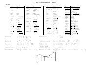
4.4 Available symbols<br />
The following tables list a number of the available symbols. Some require the<br />
loading of extra packages such as latexsym <strong>and</strong> amssymb, but this has been<br />
done <strong>for</strong> you in the template so I have not noted where they are needed. On<br />
the other h<strong>and</strong> the euro symbol in Table 1 needs the package eurosym which<br />
has not been loaded on your behalf. There are many more symbols available<br />
— the document “The Not So Short Introduction to L A TEX 2ε” contains a<br />
more comprehensive list from which the following was derived/filched.<br />
19
Table 1: Non-Mathematical Symbols.<br />
These symbols can also be used in text mode.<br />
† \dag § \S c○ \copyright e \euro<br />
‡ \ddag \P £ \pounds<br />
Table 2: Math Mode Accents.<br />
â \hat{a} ǎ \check{a} ã \tilde{a} á \acute{a}<br />
à \grave{a} ȧ \dot{a} ä \ddot{a} ă \breve{a}<br />
ā \bar{a} ⃗a \vec{a} Â \widehat{A} Ã \widetilde{A}<br />
Table 3: Log-like functions.<br />
arccos \arccos deg \deg lg \lg proj lim \projlim<br />
arcsin \arcsin det \det lim \lim sec \sec<br />
arctan \arctan dim \dim lim inf \liminf sin \sin<br />
arg \arg exp \exp lim sup \limsup sinh \sinh<br />
cos \cos gcd \gcd ln \ln sup \sup<br />
cosh \cosh hom \hom log \log tan \tan<br />
cot \cot inf \inf max \max tanh \tanh<br />
coth \coth inj lim \injlim min \min lim \varliminf<br />
csc \csc ker \ker Pr \Pr lim \varlimsup<br />
Table 4: Delimiters.<br />
( ( ) ) ↑ \uparrow ⇑ \Uparrow<br />
[ [ or \lbrack ] ] or \rbrack ↓ \downarrow ⇓ \Downarrow<br />
{ \{ or \lbrace } \} or \rbrace ↕ \updownarrow ⇕ \Updownarrow<br />
〈 \langle 〉 \rangle | | or \vert ‖ \| or \Vert<br />
⌊ \lfloor ⌋ \rfloor ⌈ \lceil ⌉ \rceil<br />
/ / \ \backslash . (dual. empty)<br />
20
Table 5: Lowercase Greek Letters.<br />
α \alpha θ \theta o o υ \upsilon<br />
β \beta ϑ \vartheta π \pi φ \phi<br />
γ \gamma ι \iota ϖ \varpi ϕ \varphi<br />
δ \delta κ \kappa ρ \rho χ \chi<br />
ɛ \epsilon λ \lambda ϱ \varrho ψ \psi<br />
ε \varepsilon µ \mu σ \sigma ω \omega<br />
ζ \zeta ν \nu ς \varsigma<br />
η \eta ξ \xi τ \tau<br />
Table 6: Uppercase Greek Letters.<br />
Γ \Gamma Λ \Lambda Σ \Sigma Ψ \Psi<br />
∆ \Delta Ξ \Xi Υ \Upsilon Ω \Omega<br />
Θ \Theta Π \Pi Φ \Phi<br />
Table 7: BIG Operators.<br />
∑ ⋃ ∨ ⊕ \sum \bigcup \bigvee \bigoplus<br />
∏ ⋂ ∧ ⊗ \prod \bigcap \bigwedge \bigotimes<br />
∐ ⊔ ⊙ \coprod \bigsqcup \bigodot<br />
∫<br />
∮<br />
⊎<br />
\int \oint<br />
\biguplus<br />
Table 8: Arrows.<br />
← \leftarrow or \gets ←− \longleftarrow ↑ \uparrow<br />
→ \rightarrow or \to −→ \longrightarrow ↓ \downarrow<br />
↔ \leftrightarrow ←→ \longleftrightarrow ↕ \updownarrow<br />
⇐ \Leftarrow ⇐= \Longleftarrow ⇑ \Uparrow<br />
⇒ \Rightarrow =⇒ \Longrightarrow ⇓ \Downarrow<br />
⇔ \Leftrightarrow ⇐⇒ \Longleftrightarrow ⇕ \Updownarrow<br />
↦→ \mapsto ↦−→ \longmapsto ↗ \nearrow<br />
←↪ \hookleftarrow ↩→ \hookrightarrow ↘ \searrow<br />
↼ \leftharpoonup ⇀ \rightharpoonup ↙ \swarrow<br />
↽ \leftharpoondown ⇁ \rightharpoondown ↖ \nwarrow<br />
⇋ \rightleftharpoons ⇐⇒ \iff (bigger spaces) ❀ \leadsto<br />
21
Table 9: Binary Relations.<br />
You can produce corresponding negations by adding a \not comm<strong>and</strong> as<br />
prefix to the following symbols, e.g. \not\sim gives ≁<br />
< < > > = =<br />
≤ \leq or \le ≥ \geq or \ge ≡ \equiv<br />
.<br />
≪ \ll ≫ \gg<br />
= \doteq<br />
≺ \prec ≻ \succ ∼ \sim<br />
≼ \preceq ≽ \succeq ≃ \simeq<br />
⊂ \subset ⊃ \supset ≈ \approx<br />
⊆ \subseteq ⊇ \supseteq ∼ = \cong<br />
⊏ \sqsubset ⊐ \sqsupset ✶ \Join<br />
⊑ \sqsubseteq ⊒ \sqsupseteq ⊲⊳ \bowtie<br />
∈ \in ∋ \ni , \owns ∝ \propto<br />
⊢ \vdash ⊣ \dashv |= \models<br />
| \mid ‖ \parallel ⊥ \perp<br />
⌣ \smile ⌢ \frown ≍ \asymp<br />
: : /∈ \notin ≠ \neq or \ne<br />
Table 10: Binary Operators.<br />
+ + − -<br />
± \pm ∓ \mp ⊳ \triangleleft<br />
· \cdot ÷ \div ⊲ \triangleright<br />
× \times \ \setminus ⋆ \star<br />
∪ \cup ∩ \cap ∗ \ast<br />
⊔ \sqcup ⊓ \sqcap ◦ \circ<br />
∨ \vee , \lor ∧ \wedge , \l<strong>and</strong> • \bullet<br />
⊕ \oplus ⊖ \ominus ⋄ \diamond<br />
⊙ \odot ⊘ \oslash ⊎ \uplus<br />
⊗ \otimes ○ \bigcirc ∐ \amalg<br />
△ \bigtriangleup ▽ \bigtriangledown † \dagger<br />
✁ \lhd ✄ \rhd ‡ \ddagger<br />
✂ \unlhd ☎ \unrhd ≀ \wr<br />
22
Table 11: Miscellaneous Symbols.<br />
. . . \dots · · · \cdots . \vdots<br />
. . . \ddots<br />
\hbar ı \imath j \jmath l \ell<br />
R \Re I \Im ℵ \aleph ℘ \wp<br />
∀ \<strong>for</strong>all ∃ \exists \mho ∂ \partial<br />
′<br />
’ ′ \prime ∅ \emptyset ∞ \infty<br />
∇ \nabla △ \triangle ✷ \Box ✸ \Diamond<br />
√<br />
⊥ \bot ⊤ \top ∠ \angle<br />
\surd<br />
♦ \diamondsuit ♥ \heartsuit ♣ \clubsuit ♠ \spadesuit<br />
¬ \neg or \lnot ♭ \flat ♮ \natural ♯ \sharp<br />
Table 12: AMS Miscellaneous.<br />
\hbar ħ \hslash k \Bbbk<br />
□ \square \blacksquare S \circledS<br />
△ \vartriangle \blacktriangle ∁ \complement<br />
▽ \triangledown \blacktriangledown \Game<br />
♦ \lozenge \blacklozenge ⋆ \bigstar<br />
∠ \angle ∡ \measuredangle ∢ \sphericalangle<br />
\diagup \diagdown \backprime<br />
∄ \nexists Ⅎ \Finv ∅ \varnothing<br />
ð \eth \mho<br />
You will find that within a short time of using L A TEX/<strong>WinEdt</strong> that you<br />
begin to remember the names of the symbols that you use most commonly.<br />
Moreover, rather than have to keep looking at this document or some other<br />
source <strong>for</strong> less frequently used symbols you can make use of tool bars that list<br />
a lot of these. If these bars are not visible then click on the Options folders,<br />
then Appearance, <strong>and</strong> check the Show GUI Page Control.<br />
5 Cross-referencing; bibliographies<br />
All scientific documents place themselves in context by citing related work<br />
<strong>and</strong> source materials, <strong>and</strong> also aid their readers by the use of (internal) crossreferencing.<br />
Both of these tasks are easily accomplished using L A TEX, in a<br />
manner that is also painless when it comes to editing.<br />
23
5.1 Internal cross-references<br />
When you run L A TEX on your file MyFile.tex another file is produced called<br />
MyFile.aux. This contains a lot of in<strong>for</strong>mation about the location of various<br />
parts <strong>and</strong> structures of your document. Some in<strong>for</strong>mation is placed into the<br />
file automatically, other parts you have to tell L A TEX to write there, but all<br />
is then available the next time you compile your document.<br />
In<strong>for</strong>mation that is automatically added to the file includes the page<br />
number where each section, subsection etc. begins, along with the number<br />
of that section. For most other items you need to place a marker at the<br />
point you wish to recall. This is done by the comm<strong>and</strong> \label{marker}. To<br />
make use of this in<strong>for</strong>mation you can then use the comm<strong>and</strong>s \ref{marker},<br />
\eqref{marker} <strong>and</strong> \pageref{marker}. The first produces the number of<br />
the section (or theorem, or equation. . . ) that is being referred to, the second<br />
is really only <strong>for</strong> referring to equations, <strong>and</strong> produces the equation number<br />
in brackets, <strong>and</strong> in an upright font if you are in the middle of an italicised<br />
portion of text, <strong>and</strong> the third gives the page number of the location of the<br />
marker. For instance the code <strong>for</strong> the beginning of this particular section is<br />
\section{Cross-referencing; bibliographies}<br />
\label{referencing}<br />
<strong>and</strong> a paragraph on page 9 ends with<br />
Bibliographies are dealt with in<br />
section~\ref{referencing}.\label{referred to}<br />
The insertion of \label{referencing} allowed me to refer on page 9 to the<br />
fact that we are now in Section 5. More importantly if I were to change this<br />
document at a later stage, perhaps by introducing a new section be<strong>for</strong>e this<br />
one, then the number of this section will change. But this change is recorded<br />
in the .aux file, <strong>and</strong> the correct section number will always be given. Note<br />
also that I included the code \label{referred to} on page 9, so that in<br />
this section I would be referring back to the correct page that referred to this<br />
section...<br />
This machinery can also be used to refer to theorems, propositions, etc.,<br />
as well as particular equations. For example if we were to write<br />
\begin{thm} \label{Fermat}<br />
$x^n + y^n \neq z^n$ <strong>for</strong> all $x,y,z \in \mathbb{Z}, \ n \geq 3$<br />
\end{thm}<br />
then any use of the code Theorem~\ref{Fermat} would replace the part<br />
\ref{Fermat} by the appropriate number <strong>for</strong> the theorem. The same works<br />
24
with equations, although you should take a little care when using align <strong>and</strong><br />
gather that you put the label in the correct place. For example<br />
\begin{align}<br />
a_1& =b_1+c_1 \label{first eqn}\\<br />
a_2& =b_2+c_2-d_2+e_2 \label{second eqn}<br />
\end{align}<br />
produces<br />
a 1 = b 1 + c 1 (5.1)<br />
a 2 = b 2 + c 2 − d 2 + e 2 (5.2)<br />
<strong>and</strong> then equation~\eqref{second eqn} produces ‘equation (5.2)’.<br />
5.2 Bibliographies<br />
A bibliography is produced using the environment thebibliography, which<br />
will be the last environment in your .tex file. The beginnings of one would<br />
look like<br />
\begin{thebibliography}{99}<br />
\bibitem{Slava1} V P Belavkin, Quantum stochastic calculus <strong>and</strong><br />
quantum nonlinear filtering, \emph{J Multivariate Anal}<br />
\textbf{42} (1992), 171--201.<br />
\bibitem{EvansM} M P Evans, Existence of quantum diffusions,<br />
\emph{Probab Theory Related Fields} \textbf{81} (1989),<br />
473--483.<br />
Each item you wish to refer to is begun with the \bibitem comm<strong>and</strong> (cf. the<br />
\item comm<strong>and</strong>s used in lists from subsection 3.6), <strong>and</strong> the text in brackets<br />
after the \bibitem gives the marker with which you will refer to the work.<br />
This produces an ordered list of the works that you are referencing, numbered<br />
1., 2. etc. To cite one of these works you then type something of the <strong>for</strong>m<br />
\cite{Slava1} to refer to the first work above, or \cite[p.480]{EvansM}<br />
if you wished to refer to page 480 of the second work. You can cite multiple<br />
works by putting a comma separated list of markers inside the curly brackets.<br />
If you prefer you can change the labelling of your bibliography — <strong>for</strong> the<br />
above you might use something like [Bel] <strong>and</strong> [Eva], or [B 92] <strong>and</strong> [E 89] to<br />
indicate the name <strong>and</strong>/or year of publication. This is achieved by changing<br />
the \bibitem comm<strong>and</strong>s above to \bibitem[Bel]{Slava1} etc. Also, the<br />
{99} that appears in the first line is an indication of what your largest label<br />
25
in the bibliography will be. Using 99 <strong>for</strong> st<strong>and</strong>ard numbered labels normally<br />
suffices (unless you’ve been reading very widely. . . ), but something like [MMM]<br />
would be better <strong>for</strong> three letter labelling.<br />
6 Further possibilities<br />
This document barely scratches the surface of what is possible within L A TEX,<br />
but should cover most of what you need <strong>for</strong> your project write-up. Most<br />
obviously I have left out all discussion about changing the layout, type size,<br />
font etc. as this would take you further from the goal of producing a report<br />
in a short space of time that conveys your researches of the last few months.<br />
References [1, 3, 4] can be consulted <strong>for</strong> more in<strong>for</strong>mation if you are interested<br />
(at a later date. . . )<br />
Many of the further extensions are achieved by loading additional package.<br />
We are already using some packages produced by the American Mathematical<br />
Society, <strong>and</strong> many more are available already on the computers in<br />
the lab. It is possible to find the relevant documentation there, or, possibly<br />
more easily, by googling <strong>for</strong> it. For example commutative diagrams such as<br />
X 0<br />
f<br />
ϕ<br />
X 1 g<br />
X 2<br />
θ<br />
<br />
Y 1 Y 2<br />
µ<br />
<br />
Z 2<br />
can be produced by the XY-pic package. Searching <strong>for</strong> xypic produces a whole<br />
host of resources.<br />
Similarly using either of the graphics or graphicx packages allows you<br />
to include graphics in your work. If you want to produce postscript output<br />
then the graphics to be included should be in encapsulated postscript <strong>for</strong>mat<br />
(i.e. as an .eps file); <strong>for</strong> pdf output they should be put in as a .pdf file. It<br />
is possible to save the plots from programs such as Maple as .eps files, <strong>and</strong><br />
conversion from that to .pdf is possible with the program epstopdf, which<br />
you can run at the comm<strong>and</strong> prompt.<br />
Once you have the line \usepackage{graphicx} in your preamble, the<br />
comm<strong>and</strong> \includegraphics[options]{filename} at the required point<br />
inserts your file. Some useful options that can be given include:<br />
• scale=1.5 — increases all linear dimensions by 1.5. The factor can be<br />
varied. . .<br />
26
• angle=90 — rotate through 90 degrees, measured anti-clockwise.<br />
• height=100mm — if you want to fix the height. Acceptable units include<br />
mm, cm, in <strong>and</strong> pt. The width option works similarly.<br />
You may want to adjust the horizontal <strong>and</strong> vertical positioning of you figure,<br />
which can be done simply with the \hspace <strong>and</strong> \vspace comm<strong>and</strong>s<br />
respectively. If you want to have side-by-side graphics with captions etc.,<br />
then you may have to learn about the figure <strong>and</strong> minipage environments,<br />
<strong>and</strong> similar constructs — google <strong>for</strong> graphicx <strong>for</strong> more in<strong>for</strong>mation.<br />
References<br />
[1] The Not So Short Introduction to L A TEX 2ε, Tobias Oetiker et. al., 2002.<br />
[2] User’s Guide <strong>for</strong> the amsmath Package (Version 2.0), American Mathematical<br />
Society, 1999.<br />
[These first two are included on the disc with the template.]<br />
[3] L A TEX: A document preparation system, Leslie Lamport, 2nd revised ed.,<br />
Addison-Wesley, Reading, MA, 1994. (686.2 LAMP)<br />
[Note: the first edition is <strong>for</strong> L A TEX 2.09, rather than the current version<br />
of L A TEX 2ε — but is still partly relevant.]<br />
[4] The L A TEX companion, Michel Goossens, Frank Mittelbach, <strong>and</strong> Alex<strong>and</strong>er<br />
Samarin, Addison-Wesley, Reading, MA, 1994. (686.2 GOOS)<br />
[Note: The first edition (1994) is not a totally reliable guide <strong>for</strong> the<br />
amsmath package. I have the recently published second edition.]<br />
27