LATEX and WinEdt for MA4053
LATEX and WinEdt for MA4053
LATEX and WinEdt for MA4053

You also want an ePaper? Increase the reach of your titles
YUMPU automatically turns print PDFs into web optimized ePapers that Google loves.
L A TEX <strong>and</strong> <strong>WinEdt</strong> <strong>for</strong> <strong>MA4053</strong><br />
Stephen J Wills<br />
Abstract<br />
These notes provide a bare bones approach to the L A TEX typesetting<br />
system, <strong>and</strong> in particular using the <strong>WinEdt</strong> program to edit the<br />
final project report <strong>for</strong> the module <strong>MA4053</strong>.<br />
Contents<br />
1 What is L A TEX/TEX? 1<br />
2 Processing documents 1<br />
3 Text-only documents 3<br />
3.1 Basic file structure . . . . . . . . . . . . . . . . . . . . . . . . 3<br />
3.2 Spaces <strong>and</strong> special characters . . . . . . . . . . . . . . . . . . 3<br />
3.3 Breaking . . . . . . . . . . . . . . . . . . . . . . . . . . . . . . 4<br />
3.4 Quotes, dashes, dots <strong>and</strong> accents . . . . . . . . . . . . . . . . 5<br />
3.5 Fonts <strong>and</strong> sizing . . . . . . . . . . . . . . . . . . . . . . . . . . 5<br />
3.6 Environments . . . . . . . . . . . . . . . . . . . . . . . . . . . 6<br />
3.7 Large scale structure . . . . . . . . . . . . . . . . . . . . . . . 8<br />
3.8 Defining comm<strong>and</strong>s etc. . . . . . . . . . . . . . . . . . . . . . 9<br />
4 Inputting mathematics 10<br />
4.1 Text <strong>and</strong> math modes; spacing . . . . . . . . . . . . . . . . . . 10<br />
4.2 Basic constructs . . . . . . . . . . . . . . . . . . . . . . . . . . 11<br />
4.3 Aligning material . . . . . . . . . . . . . . . . . . . . . . . . . 16<br />
4.4 Available symbols . . . . . . . . . . . . . . . . . . . . . . . . . 19<br />
5 Cross-referencing; bibliographies 23<br />
5.1 Internal cross-references . . . . . . . . . . . . . . . . . . . . . 24<br />
5.2 Bibliographies . . . . . . . . . . . . . . . . . . . . . . . . . . . 25<br />
6 Further possibilities 26
1 What is L A TEX/TEX?<br />
L A TEXis a powerful typesetting programme developed in the 1980s by Leslie<br />
Lamport (<strong>and</strong> others), which in essence is actually just a large number of<br />
macros <strong>for</strong> use by the lower level TEX programme written by Donald Knuth.<br />
It is the package <strong>for</strong> producing documents/papers/articles in the (pure) mathematical<br />
community.<br />
Some of the advantages it has over other programmes include<br />
• High quality professional looking output.<br />
• It is (relatively) easily to create complicated mathematical <strong>for</strong>mulae.<br />
• Cross-referencing <strong>and</strong> bibliographies can be achieved painlessly.<br />
• The programs are free <strong>and</strong> available on a wide variety of plat<strong>for</strong>ms.<br />
Moreover there is continual development by a large number of enthusiasts<br />
around the world, resulting in the production of many add-on<br />
packages that increase flexibility.<br />
• The language emphasises the logical structure of the document under<br />
preparation, rather than getting too concerned with fancy fripperies. . .<br />
This last point enables us to draw an analogy with HTML, the language in<br />
which (basic) web pages are written. There the layout is left to the particular<br />
browser the page is being displayed upon, with the author of the page<br />
describing only what fundamental features should be present. A well written<br />
web page should be viewable (<strong>and</strong> readable!) on any browser.<br />
2 Processing documents<br />
When creating a document you will end up dealing with a number of different<br />
files. Most important is the input file which will be named MyFile.tex. This<br />
is a plain ASCII text file <strong>and</strong> can be generated by any text editor. In our case<br />
we shall be using <strong>WinEdt</strong>, an editor specially developed <strong>for</strong> preparing L A TEX<br />
documents, <strong>and</strong> which consequently has a few additional useful features.<br />
Some other widely used editors have similar capabilities (e.g. emacs, which<br />
is available on a large number of plat<strong>for</strong>ms), but in reality one could use<br />
Notepad or Word if one was so inclined.<br />
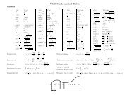
Having produced the .tex file, one then has two routes depending on the<br />
type of output required, as summarised in figure 1.<br />
1
Have idea<br />
use text editor<br />
.tex file<br />
run L A TEX<br />
run pdfL<br />
<br />
A TEX<br />
<br />
.dvi file<br />
.pdf file<br />
run dvips <br />
.ps file<br />
Figure 1: Steps in the production of a document<br />
Route 1: Be<strong>for</strong>e the introduction of pdf files there was only postscript, as<br />
understood by printers. By running L A TEX on the .tex file, a .dvi file is<br />
produced, which can be viewed, enabling any editing that is necessary<br />
be<strong>for</strong>e it is converted to postscript using dvips, <strong>and</strong> then sent to the<br />
printer. Both the compilation to .dvi <strong>and</strong> conversion to .ps can be<br />
accomplished by clicking on the relevant buttons in <strong>WinEdt</strong>.<br />
In fact this last step of conversion is largely superfluous in day-to-day<br />
use since it is possible to print from YAP, the default application <strong>for</strong><br />
viewing .dvi files.<br />
Route 2: Nowadays one can produce a pdf file direct from the .tex input<br />
by using the programme pdfL A TEX. Again this is done by a single click<br />
in <strong>WinEdt</strong>.<br />
With either route you will end up with a number other files produced as<br />
L A TEX deals with your document, <strong>and</strong> <strong>for</strong> the most part you will not need to<br />
do anything with these. Two that will definitely turn up are MyFile.aux <strong>and</strong><br />
MyFile.log. The first contains a lot of in<strong>for</strong>mation about where equations<br />
<strong>and</strong> sections in your document are to be found — this is discussed further<br />
in Section 5. The second contains a record of all the things L A TEX had to<br />
say about the processing, in particular it contains any error messages that<br />
turn up. These helpfully list the line number in your .tex file that created<br />
the error which helps you to track down what is wrong — with the aid<br />
of the somewhat cryptic error message. Most often it is a missing $ or },<br />
or one environment is ended by another, through incorrect nesting or just<br />
plain <strong>for</strong>getting to finish the previous environment. These comments should<br />
become more clear as we progress. . .<br />
There is an alternative editor to be found on the School’s computers,<br />
namely Scientific Workplace (or Word, the beefed up version). This is the<br />
2
esult of an attempt to produce a WYSIWYG version of L A TEX that feels<br />
a bit more like Microsoft Word. You are still editing L A TEX code, but it is<br />
hidden from you — you see something closer to the final product as you type.<br />
This has some advantages in that you do not have to learn so much about<br />
L A TEX at the outset, but in my opinion any such advantage is out-weighed by<br />
various disadvantages (it produces clunky code, moreover if you want to send<br />
the code to a native L A TEX user you need to do some fiddling; it is harder to<br />
make changes in overall style/control of the document; it is expensive. . . )<br />
3 Text-only documents<br />
3.1 Basic file structure<br />
The .tex file is (essentially) always of the <strong>for</strong>m<br />
\documentclass[options]{article}<br />
preamble<br />
\begin{document}<br />
text of document<br />
\end{document}<br />
Here the first line marks out the fact that we are dealing with a L A TEX 2ε<br />
document, <strong>and</strong> that we are writing an article. The part options will contain<br />
a number of possibilities, e.g. whether we are using A4 paper, want<br />
the equation number to appear on the left or right, etc. Next comes the<br />
preamble to the file, rather than the article. That is, we next supply any<br />
further instructions that will be in <strong>for</strong>ce throughout the document such as<br />
user defined comm<strong>and</strong>s, or requesting the loading of packages. The template<br />
I have supplied to you contains a lot of stuff set up here already. Finally, the<br />
actually text is enclosed by the \begin{document}. . . \end{document} pair.<br />
3.2 Spaces <strong>and</strong> special characters<br />
The amount of space between words in a .tex document is largely irrelevant<br />
<strong>and</strong> ignored. For instance<br />
Nicely typed input<br />
<strong>and</strong><br />
Nicely typed input<br />
both produce the same input. What is important is that a blank line indicates<br />
the end of the current paragraph. So while the two inputs above both produce<br />
3
Nicely typed input<br />
if we typed<br />
Nicely<br />
typed input<br />
instead we would get<br />
Nicely<br />
typed input<br />
Because of their use <strong>for</strong> comm<strong>and</strong>s etc., the following will not print as you<br />
would expect<br />
\ & % { } ^ _ # $ ~<br />
If you want to use any of the first nine of these symbols in some text or<br />
mathematics you must instead enter<br />
\backslash \& \% \{ \} \^ \_ \# \$<br />
respectively.<br />
3.3 Breaking<br />
L A TEX is programmed to work very hard to find the optimal place to break<br />
lines, pages etc., <strong>and</strong> so you are advised to leave it to get on with this task.<br />
However, when preparing the final version of you document, if you are not<br />
happy with a particular break, or if L A TEX cannot find a good place to break<br />
a line <strong>and</strong> needs help, then the following comm<strong>and</strong>s should be used:<br />
\\ \newline \newpage \pagebreak[n]<br />
The first two break the current line, <strong>and</strong> start the next without indentation.<br />
The final two break the page, with the first one leaving all text on the page<br />
where the break takes place together, the final one trying to spread the text<br />
out to fill the space. The n should be replaced with a number 0. . . 4 depending<br />
on how much you want the break to take place (4 being the strongest request).<br />
If you use long <strong>and</strong>/or unusual words then L A TEX may not know hoe to<br />
hyphenate it, <strong>and</strong> can be taught by input of the <strong>for</strong>m sjam\-bok, the symbols<br />
\- showing where a break is permissible. If the unusual word will be used<br />
repeatedly then put \hyphenation{sjam-bok} in the preamble.<br />
One place where typesetting conventions dictate that linebreaks should<br />
not take place is when a particular numbered Theorem or similar is being<br />
referred to. For instance there should not be a break between the 1 <strong>and</strong> the<br />
word Theorem when you type Theorem 1. To prevent this insert ~ between<br />
them, i.e. Theorem~1.<br />
4
3.4 Quotes, dashes, dots <strong>and</strong> accents<br />
Shift+2 should not be used to produce quotation marks. Instead <strong>for</strong> a single<br />
opening quotation mark use the symbol ‘ (found in the top-left of the<br />
keyboard) <strong>and</strong> a closing quotation mark is produced with ’. For double quotation<br />
marks use two of each! The difference between this <strong>and</strong> an erroneous<br />
use of shift+2 is shown by:<br />
”Bad quote” <strong>and</strong> “Good quote”<br />
Other important symbols are hyphens <strong>and</strong> dashes. There are three separate<br />
types of dash: an intraword dash, a numerical range, <strong>and</strong> a dash indicating a<br />
pause in the sentence. These are given by 1, 2 <strong>and</strong> 3 copies of - respectively.<br />
For example<br />
bye-law 1–10 <strong>and</strong> That is true — in this case.<br />
are produced by<br />
bye-law 1--10 That is true --- in this case.<br />
An ellipsis (the symbol . . . ) is produced with \ldots, since typing .<br />
three times produces ... which does not have the correct spacing.<br />
Accented letters such as ã, é <strong>and</strong> ô can be produced by the inputs \~{a},<br />
\’{e} <strong>and</strong> \^{o}.<br />
3.5 Fonts <strong>and</strong> sizing<br />
By default L A TEX documents are set in Computer Modern fonts, which look<br />
fine <strong>and</strong> I would not encourage you to go down the route of trying to change<br />
this. Times Roman, Courier, etc. are available, as are a myriad of <strong>for</strong>eign<br />
scripts (Russian, Korean,. . . ). More important at the moment is the ability<br />
to emphasis words <strong>and</strong> change size. The follow comm<strong>and</strong>s achieve a change<br />
in the shape:<br />
\textit Italics \textbf Bold face<br />
\textup Upright \textrm Roman<br />
\textsf Sans serif \texttt Typewriter style<br />
They can be combined in obvious ways. For example bold sans serif is<br />
achieved by typing \textbf{\textsf{bold sans serif}}. Most of the<br />
time the default is <strong>for</strong> roman upright text so these two comm<strong>and</strong>s are not<br />
immediately useful, except in the statements of theorems <strong>and</strong> the like, when<br />
the default is italics. There is another comm<strong>and</strong>, \emph, that can be used to<br />
emphasis text. In general this achieves the same effect as using \textit, but<br />
5
the philosophical point is that you should be able to make a global change at<br />
a latter stage if you decided <strong>for</strong> instance that emphasis would be better generated<br />
by bold sans serif or underlined typewriter style. See the subsection<br />
on defining comm<strong>and</strong>s later on <strong>for</strong> more in<strong>for</strong>mation.<br />
To change the size of text there are the following comm<strong>and</strong>s, in order of<br />
decreasing size:<br />
\tiny \scriptsize \footnotesize \small<br />
\normalsize \large \Large \LARGE<br />
\huge \Huge<br />
For example the input<br />
{\Large Starting big} <strong>and</strong> {\small getting} {\tiny smaller}<br />
produces<br />
Starting big <strong>and</strong> getting smaller<br />
3.6 Environments<br />
To insert lists, theorems, tables etc. requires the use of the appropriate environment.<br />
The text <strong>for</strong> such an object is enclosed in a \begin{environment}<br />
\end{environment} pair. For example there are three default styles of list<br />
which are itemize, enumerate <strong>and</strong> description. The first produces bullet<br />
points or equivalent <strong>for</strong> each item in the list, the second numbers the entries,<br />
<strong>and</strong> the third permits user defined labelling. For example the list<br />
1. Item 1<br />
2. Item 2<br />
3. Item 3<br />
is produced by<br />
\begin{enumerate}<br />
\item Item 1<br />
\item Item 2<br />
\item Item 3<br />
\end{enumerate}<br />
These lists can be successively nested, giving rise to new numbering or bulleting<br />
styles in the different levels. For example two layers of enumerate<br />
gives<br />
6
1. Item 1<br />
(a) Subitem 1 of first item<br />
(b) Subitem 2 of first item<br />
2. Item 2<br />
The st<strong>and</strong>ard labelling in itemize <strong>and</strong> enumerate can be overridden by input<br />
of the <strong>for</strong>m \item[New label], <strong>and</strong> this is how the user defined labels are<br />
given in the description environment. Two further list types are provided<br />
by the template which are both variants on the enumerate environment. One<br />
is alist which labels the items (a), (b) etc., <strong>and</strong> the other is ilist which<br />
labels the items (i), (ii) etc. These save having to type \item[(a)] etc.<br />
The center environment <strong>and</strong> quote environment are useful <strong>for</strong> displaying<br />
tables <strong>and</strong> quotes in text documents. To produce tables use the tabular<br />
environment. This begins with a comm<strong>and</strong> like \begin{tabular}[cr|lr|],<br />
where the letters l, c <strong>and</strong> r indicate the number of columns <strong>and</strong> whether<br />
the entries should be left justified, centred or right justified. An upright line<br />
indicates that there should be a vertical line separating the columns. To<br />
insert horizontal lines use \hline at the end of the preceding line of entries.<br />
The entries themselves are separated into the relevant columns by & in the<br />
input, <strong>and</strong> the end of the line is indicated by \\. For example the input<br />
\begin{center}<br />
\begin{tabular}{|c|lr} \hline<br />
{\large Centred} & {\large left} & {\large right} \\<br />
{\small centred} & {\small left} & {\small right} \\ \hline<br />
\end{tabular}<br />
\end{center}<br />
produces<br />
Centred left right<br />
centred left right<br />
Not enclosing the tabular environment in the center environment will cause<br />
the table to be set in the middle of the current paragraph.<br />
The most important environments that you will need <strong>for</strong> the project write<br />
up are the so-called theorem-like environments. Since it is impossible to know<br />
from the outset what is required in a given document in terms of theorems,<br />
propositions etc., there is a means by which the user specifies the types<br />
required in the preamble of the document. I have done this in the given<br />
template, creating the following environments:<br />
7
thm propn lemma cor defn note rem rems<br />
<strong>for</strong> producing a Theorem, Proposition, Lemma, Corollary, Definition, Note,<br />
Remark or Remarks respectively. The first five will also produce numbering,<br />
<strong>and</strong> are numbered consecutively together. It is possible to have Theorems<br />
numbered on one scale, Propositions under another etc. The first four italicise<br />
the text inside them, <strong>and</strong> the final four leave it upright.<br />
So the inputs<br />
\begin{thm} \begin{rem}<br />
$E = mc^2$ General relativity is complicated<br />
\end{thm}<br />
\end{rem}<br />
produce<br />
Theorem 3.1. E = mc 2<br />
<strong>and</strong><br />
Remark. General relativity is complicated<br />
respectively. The differing possibilities <strong>for</strong> italic text, bold or italicised labeling<br />
etc., are implemented by AMS-L A TEX, which also provides as st<strong>and</strong>ard<br />
the proof environment. This writes Proof. at the start of your proof <strong>and</strong><br />
the symbol at the end.<br />
3.7 Large scale structure<br />
Any document tends to have a large scale structure starting with front matter<br />
(such as a title, author <strong>and</strong> so on) be<strong>for</strong>e splitting the document into chapters,<br />
sections, etc., possibly with appendices, <strong>and</strong> then ending with a bibliography<br />
<strong>and</strong> maybe an index.<br />
The front matter <strong>for</strong> your project can be achieved by filling in the blanks<br />
in<br />
\title{}<br />
\author{}<br />
\maketitle<br />
\begin{abstract}<br />
\end{abstract}<br />
which appears just after the \begin{document} comm<strong>and</strong>.<br />
The appropriate divisions within a document are produced by comm<strong>and</strong>s<br />
such as<br />
8
\chapter \section \subsection \subsubsection<br />
— this section was started by the input \section{Text-only documents}.<br />
In fact the comm<strong>and</strong>s available depend on the declaration of document type<br />
contained in the \documentclass line at the start of your .tex file. I have set<br />
up the template as an article, so the highest level section is in fact section,<br />
rather than chapter. L A TEX also generates the numbers here automatically,<br />
although it is possible to control just how far down the parts are labelled<br />
through use of the \secnumdepth comm<strong>and</strong>. Bibliographies are dealt with<br />
in section 5.<br />
3.8 Defining comm<strong>and</strong>s etc.<br />
When producing a document it is common to find that certain constructs are<br />
used repeatedly, <strong>and</strong> it would involve a lot of repetitive typing each time the<br />
construct appears. Time can be saved by creating user defined comm<strong>and</strong>s<br />
in the preamble. For example in one set of lecture notes that I prepared I<br />
decided that any term that was being defined should be set in bold sans serif,<br />
which normally would involve typing \textbf{\textsf{term}} each time.<br />
Instead I included the line<br />
\newcomm<strong>and</strong>{\dn}[1]{\textbf{\textsf{#1}}<br />
in the preamble. The \dn in the curly brackets indicates that I am defining<br />
a comm<strong>and</strong> called dn. The 1 in the square brackets indicates that there is<br />
to be one input into the comm<strong>and</strong>. Finally, the actual comm<strong>and</strong> appears<br />
enclosed in the final set of brackets, with the #1 indicated the point where<br />
the (first) input should be used. So now \dn{topological space} produces<br />
topological space. A philosophical viewpoint on the use of such constructs<br />
is that if at a later stage I decide to change how a defined term is displayed<br />
then I need only change the definition of the comm<strong>and</strong> \dn.<br />
If you try to create a comm<strong>and</strong> with a name that is already in use then<br />
L A TEX will complain. If you really want to use that name then there is the<br />
\renewcomm<strong>and</strong> but this is a somewhat dangerous path to go down. It is<br />
not necessary to have inputs in the comm<strong>and</strong>. For example rather than<br />
type \begin{thm} <strong>and</strong> \end{thm} at the beginning <strong>and</strong> end of each of your<br />
theorems you could put<br />
\newcomm<strong>and</strong>{\bt}{\begin{thm}}<br />
\newcomm<strong>and</strong>{\et}{\end{thm}}<br />
in the preamble, <strong>and</strong> then need only type \bt <strong>and</strong> \et. You can also create<br />
new environments in a similar way.<br />
9
4 Inputting mathematics<br />
4.1 Text <strong>and</strong> math modes; spacing<br />
There are two main modes in which L A TEX works. So far we have only made<br />
use of text mode, but more importantly there is also math mode used <strong>for</strong><br />
inputting mathematics — the reason we are dealing with the program in the<br />
first place! There are two ways of including mathematics in a document. It<br />
can either be placed in-line, that is in the middle of the paragraph, or can<br />
be displayed. The first is used <strong>for</strong> relatively small portions of mathematics,<br />
in particular if they are not being emphasised. For large equations or <strong>for</strong><br />
emphasis one should use displayed equations.<br />
Mathematical text within a paragraph is obtained by enclosing the required<br />
comm<strong>and</strong>s between $ <strong>and</strong> $, or \( <strong>and</strong> \), or between \begin{math}<br />
<strong>and</strong> \end{math}. So <strong>for</strong> instance<br />
And Pythagoras said $x^2+y^2=z^2$, <strong>and</strong> all was right-angled.<br />
produces<br />
And Pythagoras said x 2 + y 2 = z 2 , <strong>and</strong> all was right-angled.<br />
On the other h<strong>and</strong>, if we wanted to emphasis the equation then the mathematics<br />
should appear between \begin{equation} <strong>and</strong> \begin{equation}<br />
if the equation is to be numbered, or between \[ <strong>and</strong> \], or $$ <strong>and</strong> $$,<br />
or \begin{displaymath} <strong>and</strong> \end{displaymath}, or \begin{equation*}<br />
<strong>and</strong> \end{equation*} if the equation is not to be numbered. So our example<br />
above could be entered as<br />
And Pythagoras said<br />
\[<br />
x^2+y^2=z^2,<br />
\]<br />
<strong>and</strong> all was right-angled.<br />
to produce<br />
And Pythagoras said<br />
<strong>and</strong> all was right-angled.<br />
x 2 + y 2 = z 2 ,<br />
Letters appearing in math mode are processed by L A TEX as if they are<br />
variables, <strong>and</strong> are usually typeset in italics. However the spacing between<br />
them differs from that in text mode, <strong>and</strong> so a $. . . $ should not be used as a<br />
10
shorth<strong>and</strong> <strong>for</strong> \textit. For example \textit{different} <strong>and</strong> $different$<br />
produce the outputs different <strong>and</strong> different respectively.<br />
It is common to have a few words in a given <strong>for</strong>mula. Indeed, certain<br />
journals are keen that the symbol ∀ should not appear in definitions <strong>and</strong><br />
displayed equations, but should be replaced by ‘<strong>for</strong> all’. When dealing with<br />
in-line mathematics you could come out of math mode <strong>and</strong> re-enter it after<br />
the text part is dealt with. This is not possible in displayed equations, nor in<br />
some circumstances with in-line mathematics. A more robust way of doing<br />
things is to enclose the text part inside \text{. . . }. For example<br />
\begin{equation}<br />
\exists x,y,z \in \mathbb{Z} \text{such that}<br />
x^{101}+y^{101}=z^{101}<br />
\end{equation}<br />
produces<br />
∃x, y, z ∈ Zsuch thatx 101 + y 101 = z 101 (4.1)<br />
This example illustrates another problem/feature of entering mathematics.<br />
As with text mode, spaces between parts of the input are ignored.<br />
Indeed, in math mode they do not even produce a space. One remedy in<br />
the above would be to change \text{such that} to \text{ such that },<br />
since the spaces inside the \text comm<strong>and</strong> are processed in text mode <strong>and</strong><br />
so are not ignored. There can be a need to alter/adjust the spacing between<br />
mathematics <strong>and</strong> comm<strong>and</strong>s <strong>for</strong> doing this include, in increasing order<br />
\! thin negative space \, thin space<br />
\: medium space \; thick space<br />
\␣ interword space \quad space width of M<br />
\qquad biggest space<br />
4.2 Basic constructs<br />
The following are a non-exhaustive list of common constructs in mathematics,<br />
<strong>and</strong> how to obtain them in L A TEX.<br />
Super- <strong>and</strong> subscripts<br />
These are produced by ^ <strong>and</strong> _ respectively. For example the inputs $x^2$<br />
<strong>and</strong> $a_{13}$ produce x 2 <strong>and</strong> a 13 . Note that the curly brackets are required<br />
around the 13 to ensure that both numbers are used as the subscript. Without<br />
them we get a 1 3.<br />
11
Roots<br />
$\sqrt{x}$ produces √ x. To take nth roots use $\sqrt[n]{x+iy}$ to get<br />
n√ x + iy.<br />
Lines, braces, accents<br />
To get a line over the top of some mathematics, enclosed the required code<br />
inside \overline{...}. For example $\overline{x+iy} = x-iy$ produces<br />
x + iy = x − iy. The comm<strong>and</strong> \underline works similarly. There are also<br />
the comm<strong>and</strong>s \overbrace <strong>and</strong> \underbrace which can be combined usefully<br />
with super- <strong>and</strong> subscripts. For example<br />
is produced by<br />
m<br />
m<br />
(a m ) n { }} { { }} {<br />
= ( a · · · a) · · · ( a · · · a)<br />
} {{ }<br />
n<br />
\[<br />
(a^m)^n = \underbrace{(\overbrace{a \cdots a}^m) \cdots<br />
(\overbrace{a \cdots a}^m)}_n<br />
\]<br />
A number of different accents are possible, <strong>for</strong> example âb, ˜T <strong>and</strong> so, as<br />
shown in Table 2. The \widehat <strong>and</strong> \widetilde are reasonably stretchy,<br />
but do have their limits.<br />
Greek <strong>and</strong> other symbols<br />
The Greek alphabet begins α, β, γ,. . . , <strong>and</strong> is produced by \alpha etc. For<br />
uppercase Greek letters change the first letter in the comm<strong>and</strong> to uppercase.<br />
For example $\Gamma$ gives Γ, noting that an uppercase alpha is just A,<br />
given by $A$. Note also that some letters have variants. See Tables 5 <strong>and</strong> 6.<br />
Infinity is given by \infty. There are further variants on the ellipsis<br />
\ldots discussed earlier, which are \cdots (· · · ), \cdot (·), \vdots (.) <strong>and</strong><br />
\ddots ( . ..). Unlike \ldots these variants only work in math mode. The<br />
final two are useful in particular when typesetting large matrices.<br />
Integrals, sums <strong>and</strong> products<br />
These are produced by \int, \sum <strong>and</strong> \prod. The ranges are given by<br />
the appropriate sub- <strong>and</strong> superscripts. For instance ∑ n<br />
i=1 i = 1 n(n + 1)<br />
2<br />
is produced by $\sum_{i=1}^n i = \frac{1}{2} n(n+1)$. These symbols<br />
12
have different sizes <strong>and</strong> place the limits in different places depending on<br />
whether they are used in-line or in a display. For instance when the previous<br />
example is displayed we get<br />
n∑<br />
i=1<br />
i = 1 n(n + 1)<br />
2<br />
where the sum is now given by a bigger symbol <strong>and</strong> the limits are placed on<br />
top <strong>and</strong> bottom, rather than to the side. This can be altered by h<strong>and</strong> — see<br />
the section below.<br />
Multiple integrals can either be achieved by repeating \int the required<br />
number of times (<strong>and</strong> using \! to get better spacing), or, if there is only one<br />
subscript giving the range of integration, then \iint, \iiint, \iiiint <strong>and</strong><br />
\idotsint give ∫∫ , ∫∫∫ , ∫∫∫∫ <strong>and</strong> ∫ ··· ∫ , where the spacing between the<br />
integral signs is done automatically.<br />
Set <strong>and</strong> vector space operations<br />
Unions, intersections <strong>and</strong> set differences are given by the comm<strong>and</strong>s \cup,<br />
\cap <strong>and</strong> \setminus when dealing with a given (finite) numbers of sets.<br />
For unions <strong>and</strong> intersections of families of sets use \bigcup <strong>and</strong> \bigcap.<br />
For example A ∪ B <strong>and</strong> ⋂ ∞<br />
i=1 A i are given respectively by $A \cup B$ <strong>and</strong><br />
$\bigcap_{i=1}^\infty A_i$.<br />
Direct sums (⊕) are given by \oplus, <strong>and</strong> tensor products (⊗) are given<br />
by \otimes, <strong>and</strong> again both of these have the larger variants \bigoplus <strong>and</strong><br />
\bigotimes <strong>for</strong> use on families of vector spaces, rings etc.<br />
As with integrals, the big versions of all of these symbols behave differently<br />
when in displays, compared to in-line use.<br />
Text <strong>and</strong> display styles<br />
Sometimes the change in behaviour concerning placing of limits <strong>and</strong>/or the<br />
size of the symbol <strong>for</strong> comm<strong>and</strong>s such as \int <strong>and</strong> \bigcup are not what you<br />
want to happen. This behaviour can be over-ruled by use of the \textstyle<br />
<strong>and</strong> \displaystyle comm<strong>and</strong>s which change it to the named variety. For<br />
example normally $\bigcup_{i=1}^n A_i$ produces ⋃ n<br />
i=1 A i, but when enclosed<br />
in a \displaystyle comm<strong>and</strong> gives A i . The relevant symbols<br />
n⋃<br />
that<br />
change are listed in Table 7.<br />
13<br />
i=1
Fractions<br />
$\frac{\pi}{2}$ produces π , although when displayed will give the larger<br />
2<br />
result π 2 . To produce textstyle fractions in displayed material either use<br />
the \textstyle comm<strong>and</strong>, or type $\tfrac{\pi}{2}$. The \binom variant<br />
provides binomial coefficients: ( 3<br />
2)<br />
is produced by $\binom{3}{2}$.<br />
Log-like functions<br />
Certain function names are usually set with upright letters, with special<br />
spacing on either side. Rather than have to fiddle around with \mathrm <strong>and</strong><br />
spacing comm<strong>and</strong>s, a number of such functions have been pre-programmed<br />
with comm<strong>and</strong> names like \log, \sin <strong>and</strong> so on — see Table 3. To create new<br />
functions you should use the \DeclareMathOperator comm<strong>and</strong>, rather than<br />
\newcomm<strong>and</strong>, since this sorts out the font type <strong>and</strong> size issues automatically.<br />
It is used in exactly the same way, <strong>for</strong> example<br />
\DeclareMathOperator{\Range}{Ran}<br />
produces Ran V when you type $\Range V$.<br />
Modulo arithmetic<br />
The AMS-L A TEX package provides the comm<strong>and</strong>s \mod, \bmod, \pmod <strong>and</strong><br />
\pod <strong>for</strong> modulo arithmetic. They produce, respectively:<br />
13 = 4 mod 9; 13 = 4 mod 9; 13 = 4 (mod 9); 13 = 4 (9)<br />
Bracketing<br />
St<strong>and</strong>ard parentheses ( <strong>and</strong> ) are given by ( <strong>and</strong> ). Similarly <strong>for</strong> square<br />
brackets [ <strong>and</strong> ]. For curly brackets you need to type \{ <strong>and</strong> }, since { <strong>and</strong> }<br />
are used throughout in giving the arguments of comm<strong>and</strong>s. Further examples<br />
of delimiters, used to give inner products or norms <strong>for</strong> example, can be found<br />
in Table 4.<br />
The size of brackets can be adjusted to accommodate large contents. For<br />
example consider<br />
(<br />
∫ t<br />
0<br />
f(t) 2 dt) 1/2<br />
<strong>and</strong><br />
(∫ t<br />
0<br />
) 1/2<br />
f(t) 2 dt<br />
The brackets in the latter are generated by \left( <strong>and</strong> \right). It is vital<br />
that there is a matching pair of \left <strong>and</strong> \right comm<strong>and</strong>s — but the<br />
14
ackets need not match each other. The comm<strong>and</strong>s \left. <strong>and</strong> \right.<br />
produce the ‘empty’ bracket.<br />
Sometimes the sizing given by \left <strong>and</strong> \right can be a bit excessive.<br />
These can be adjusted by h<strong>and</strong> by using the comm<strong>and</strong>s (in increasing order<br />
of size) \bigl, \Bigl, \biggl <strong>and</strong> \Biggl in front of the left h<strong>and</strong> bracket,<br />
<strong>and</strong> \bigr etc. in front of the right h<strong>and</strong> bracket. Moreover, these no longer<br />
need to match, which can be helpful if the brackets appear on different lines<br />
of a (broken) displayed equation.<br />
Arrays <strong>and</strong> matrices; cases<br />
The st<strong>and</strong>ard math mode version of the tabular environment discussed previously<br />
is the array environment, <strong>and</strong> works in a very similar way. In combination<br />
with brackets given by comm<strong>and</strong>s such as \left( <strong>and</strong> \right) this<br />
gives one method of producing matrices. More efficient, both to type <strong>and</strong> in<br />
terms of the horizontal space used, are the environments matrix, pmatrix,<br />
bmatrix <strong>and</strong> vmatrix from AMS-L A TEX. With these you are not required<br />
to specify in advance the number columns in your matrix, nor the relative<br />
positioning of the entries since they are all assumed to be centred. So<br />
\left( \begin{array}{ccc} 1 & 2 & 3 \\ e^1 & \log 3 & \cos 7<br />
\end{array} \right)<br />
<strong>and</strong><br />
\begin{pmatrix} 1 & 2 & 3 \\ e^1 & \log 3 & \cos 7<br />
\end{pmatrix}<br />
produce ( 1 2 3<br />
e 1 log 3 cos 7<br />
)<br />
<strong>and</strong><br />
( )<br />
1 2 3<br />
e 1 log 3 cos 7<br />
respectively.<br />
To define a function involving many cases either use the array environment<br />
inside brackets given by \left\{ <strong>and</strong> \right., or use the cases<br />
environment. For example<br />
\cos (n\pi) = \begin{cases} -1 & \text{if } n \text{ is odd} \\<br />
+1 & \text{if } n \text{ is even} \end{cases}<br />
gives<br />
cos(nπ) =<br />
{<br />
−1<br />
if n is odd<br />
+1 if n is even<br />
15
Fonts <strong>and</strong> sizes<br />
The comm<strong>and</strong>s <strong>for</strong> changing between type faces in mathematics are similar<br />
to those in <strong>for</strong> use with text. Also, there are calligraphic <strong>and</strong> blackboard<br />
bold versions of the uppercase letters, <strong>and</strong> fraktur versions of both upper<strong>and</strong><br />
lowercase letters.<br />
\mathit Italics \mathrm Roman<br />
\mathbf Boldface \mathsf Sansserif<br />
\mathtt Typewriter \mathcal CALLIGRAPHIC<br />
\mathbb BLACKboardbold \mathfrak Fraktur<br />
There are fewer sizing comm<strong>and</strong>s, <strong>and</strong> these reflect the number of levels<br />
of super- <strong>and</strong> subscripts, <strong>and</strong> whether or not one is in-line or using a<br />
display. The comm<strong>and</strong>s that change the current style are \displaystyle,<br />
\textstyle, \scriptstyle <strong>and</strong> \scriptscriptstyle. For example ordinarily<br />
$e^{y(i)}$ produces e y(i) , whereas $e^{\textstyle y(i)}}$ produces<br />
e y(i) .<br />
4.3 Aligning material<br />
It often happens that even though you are trying to display material that<br />
would look wrong in the text, your equations are too long to fit onto the one<br />
line. Alternatively you are trying to give an account of a number of steps in a<br />
calculation. The following environments give a number of options <strong>for</strong> dealing<br />
with these <strong>and</strong> other circumstances. In what follows the term equation could<br />
equally well mean inequality, or another mathematical expression involving<br />
a binary operation.<br />
If the equation you have is just too long, but there is only one equation<br />
then there are two choices: multline <strong>and</strong> split. The first is an environment<br />
in itself. Each time you want to break the line you should insert \\; the first<br />
line is placed at the left of the page, the final one shifted to the right, <strong>and</strong><br />
any intervening lines are centred. The split environment, on the other h<strong>and</strong>,<br />
has to be used inside the equation or equation* environments. Moreover it<br />
allows <strong>for</strong> alignment between the lines. Again \\ is used to denote the point<br />
to break, <strong>and</strong> & is used to indicate the points to align. Examples include<br />
\begin{multline}<br />
H_c = \frac{1}{2n} \sum^n_{l=0} (-1)^{l} (n-{l})^{p-2}<br />
\sum_{l_1 +\cdots + l_p=l} \prod^p_{i=1} \binom{n_i}{l _i} \\<br />
\cdot [(n-l )-(n_i-l _i)]^{n_i-l _i} \cdot<br />
\Bigl[(n-l )^2 - \sum^p_{j=1} (n_i-l _i)^2 \Bigr]<br />
\end{multline}<br />
16
which produces<br />
H c = 1<br />
2n<br />
n∑<br />
(−1) l (n − l) p−2<br />
l=0<br />
∑<br />
p∏<br />
l 1 +···+l p=l i=1<br />
· [(n − l) − (n i − l i )] n i−li<br />
·<br />
(<br />
ni<br />
l i<br />
)<br />
[<br />
(n − l) 2 −<br />
p∑ ]<br />
(n i − l i ) 2<br />
j=1<br />
(4.2)<br />
Here you might want the items on the second line to line up with the = sign<br />
on the line above, so could use a combination of equation <strong>and</strong> split by<br />
typing<br />
\begin{equation}<br />
\begin{split}<br />
H_c &= \frac{1}{2n} \sum^n_{l=0} (-1)^{l} (n-{l})^{p-2}<br />
\sum_{l_1 +\cdots + l_p=l} \prod^p_{i=1} \binom{n_i}{l _i} \\<br />
&\quad \cdot [(n-l )-(n_i-l _i)]^{n_i-l _i} \cdot<br />
\Bigl[(n-l )^2 - \sum^p_{j=1} (n_i-l _i)^2 \Bigr]<br />
\end{split}<br />
\end{equation}<br />
which produces<br />
H c = 1<br />
2n<br />
n∑<br />
(−1) l (n − l) p−2<br />
l=0<br />
· [(n − l) − (n i − l i )] n i−li<br />
·<br />
∑<br />
p∏<br />
l 1 +···+l p=l i=1<br />
[<br />
(n − l) 2 −<br />
(<br />
ni<br />
l i<br />
)<br />
p∑ ]<br />
(n i − l i ) 2<br />
j=1<br />
(4.3)<br />
Note that the & should come be<strong>for</strong>e the binary relation, so the = in the first<br />
line above. If there is no binary relation in any of the subsequent lines then<br />
you should have &\quad to obtain the appropriate spacing.<br />
There is an unnumbered version of multline, namely multline*, but<br />
no such thing <strong>for</strong> split. Indeed, because a split environment is meant<br />
to go inside another equation-like environment, it is the outer environment<br />
that should be unnumbered. So in our example above we should use the<br />
equation* environment.<br />
For a sequence of aligned equations there is the align environment, together<br />
with the unnumbered version align*. Again the symbol & is used to<br />
denote the alignment points. For example<br />
\begin{align}<br />
a_1 &= b_1+c_1\\<br />
17
a_2 &= b_2+c_2-d_2+e_2<br />
\end{align}<br />
produces<br />
a 1 = b 1 + c 1 (4.4)<br />
a 2 = b 2 + c 2 − d 2 + e 2 (4.5)<br />
In fact you can have (almost) any odd number of & symbols in an align<br />
environment. The odd numbered ones indicate alignment points, <strong>and</strong> the<br />
even ones separate the columns. So<br />
\begin{align*}<br />
a_{11} &= b_{11} & a_{12} &= b_{12}\\<br />
a_{21} &= b_{21} & a_{22} &= b_{22}+c_{22}<br />
\end{align*}<br />
produces<br />
a 11 = b 11 a 12 = b 12<br />
a 21 = b 21 a 22 = b 22 + c 22<br />
If you have a number of equations or expressions to display over more<br />
than one line, but do not need to align them then there are the gather <strong>and</strong><br />
gather* environments. Once more \\ give the line breaks, but should be no<br />
&s present. For example<br />
\begin{gather}<br />
a_1 = b_1+c_1\\<br />
a_2 = b_2+c_2-d_2+e_2 \notag<br />
\end{gather}<br />
produces<br />
a 1 = b 1 + c 1 (4.6)<br />
a 2 = b 2 + c 2 − d 2 + e 2<br />
All of these environments produce output that stretches across the width<br />
of the page. If you need to create a block that is as wide as the text it<br />
produces in order to insert it within further displayed material then there<br />
are the environments aligned <strong>and</strong> gathered. For example<br />
{ }<br />
−1 if n is odd<br />
cos nπ =<br />
= (−1) n<br />
+1 if n is even<br />
is produced by<br />
18
\[<br />
\cos n\pi = \left\{<br />
\begin{aligned} -1 & \text{ if } n \text{ is odd} \\<br />
+1 & \text{ if } n \text{ is even} \end{aligned}<br />
\right\} = (-1)^n<br />
\]<br />
If you have a run of aligned equations <strong>and</strong> wish to include a one or two<br />
word interjection be<strong>for</strong>e the end, whilst retaining the alignment, then there<br />
is the comm<strong>and</strong> \intertext. For example<br />
<strong>and</strong> hence<br />
is produced by<br />
x 2 = 0<br />
x 2 ≮ −10000 × 10000<br />
\begin{align*}<br />
x^2 &= 0 \\<br />
\intertext{<strong>and</strong> hence}<br />
x^2-200 &\not< -10000 \times 10000<br />
\end{align*}<br />
Suppressing <strong>and</strong> changing numbering<br />
If you are using one of the numbered equation environments but do not want<br />
every line to be numbered then insert \notag on those lines where a number is<br />
not required. On the other h<strong>and</strong> if you wish to override the current number,<br />
or supply one if you are using a starred environment then there are the<br />
comm<strong>and</strong>s \tag{n} <strong>and</strong> \tag*{..}. The first produces the number (n) <strong>for</strong><br />
the equation in question. The \tag* produces a similar effect, but without<br />
the bracketing which is useful if you wish to add adornment to that part of<br />
the labelling.<br />
4.4 Available symbols<br />
The following tables list a number of the available symbols. Some require the<br />
loading of extra packages such as latexsym <strong>and</strong> amssymb, but this has been<br />
done <strong>for</strong> you in the template so I have not noted where they are needed. On<br />
the other h<strong>and</strong> the euro symbol in Table 1 needs the package eurosym which<br />
has not been loaded on your behalf. There are many more symbols available<br />
— the document “The Not So Short Introduction to L A TEX 2ε” contains a<br />
more comprehensive list from which the following was derived/filched.<br />
19
Table 1: Non-Mathematical Symbols.<br />
These symbols can also be used in text mode.<br />
† \dag § \S c○ \copyright e \euro<br />
‡ \ddag \P £ \pounds<br />
Table 2: Math Mode Accents.<br />
â \hat{a} ǎ \check{a} ã \tilde{a} á \acute{a}<br />
à \grave{a} ȧ \dot{a} ä \ddot{a} ă \breve{a}<br />
ā \bar{a} ⃗a \vec{a} Â \widehat{A} Ã \widetilde{A}<br />
Table 3: Log-like functions.<br />
arccos \arccos deg \deg lg \lg proj lim \projlim<br />
arcsin \arcsin det \det lim \lim sec \sec<br />
arctan \arctan dim \dim lim inf \liminf sin \sin<br />
arg \arg exp \exp lim sup \limsup sinh \sinh<br />
cos \cos gcd \gcd ln \ln sup \sup<br />
cosh \cosh hom \hom log \log tan \tan<br />
cot \cot inf \inf max \max tanh \tanh<br />
coth \coth inj lim \injlim min \min lim \varliminf<br />
csc \csc ker \ker Pr \Pr lim \varlimsup<br />
Table 4: Delimiters.<br />
( ( ) ) ↑ \uparrow ⇑ \Uparrow<br />
[ [ or \lbrack ] ] or \rbrack ↓ \downarrow ⇓ \Downarrow<br />
{ \{ or \lbrace } \} or \rbrace ↕ \updownarrow ⇕ \Updownarrow<br />
〈 \langle 〉 \rangle | | or \vert ‖ \| or \Vert<br />
⌊ \lfloor ⌋ \rfloor ⌈ \lceil ⌉ \rceil<br />
/ / \ \backslash . (dual. empty)<br />
20
Table 5: Lowercase Greek Letters.<br />
α \alpha θ \theta o o υ \upsilon<br />
β \beta ϑ \vartheta π \pi φ \phi<br />
γ \gamma ι \iota ϖ \varpi ϕ \varphi<br />
δ \delta κ \kappa ρ \rho χ \chi<br />
ɛ \epsilon λ \lambda ϱ \varrho ψ \psi<br />
ε \varepsilon µ \mu σ \sigma ω \omega<br />
ζ \zeta ν \nu ς \varsigma<br />
η \eta ξ \xi τ \tau<br />
Table 6: Uppercase Greek Letters.<br />
Γ \Gamma Λ \Lambda Σ \Sigma Ψ \Psi<br />
∆ \Delta Ξ \Xi Υ \Upsilon Ω \Omega<br />
Θ \Theta Π \Pi Φ \Phi<br />
Table 7: BIG Operators.<br />
∑ ⋃ ∨ ⊕ \sum \bigcup \bigvee \bigoplus<br />
∏ ⋂ ∧ ⊗ \prod \bigcap \bigwedge \bigotimes<br />
∐ ⊔ ⊙ \coprod \bigsqcup \bigodot<br />
∫<br />
∮<br />
⊎<br />
\int \oint<br />
\biguplus<br />
Table 8: Arrows.<br />
← \leftarrow or \gets ←− \longleftarrow ↑ \uparrow<br />
→ \rightarrow or \to −→ \longrightarrow ↓ \downarrow<br />
↔ \leftrightarrow ←→ \longleftrightarrow ↕ \updownarrow<br />
⇐ \Leftarrow ⇐= \Longleftarrow ⇑ \Uparrow<br />
⇒ \Rightarrow =⇒ \Longrightarrow ⇓ \Downarrow<br />
⇔ \Leftrightarrow ⇐⇒ \Longleftrightarrow ⇕ \Updownarrow<br />
↦→ \mapsto ↦−→ \longmapsto ↗ \nearrow<br />
←↪ \hookleftarrow ↩→ \hookrightarrow ↘ \searrow<br />
↼ \leftharpoonup ⇀ \rightharpoonup ↙ \swarrow<br />
↽ \leftharpoondown ⇁ \rightharpoondown ↖ \nwarrow<br />
⇋ \rightleftharpoons ⇐⇒ \iff (bigger spaces) ❀ \leadsto<br />
21
Table 9: Binary Relations.<br />
You can produce corresponding negations by adding a \not comm<strong>and</strong> as<br />
prefix to the following symbols, e.g. \not\sim gives ≁<br />
< < > > = =<br />
≤ \leq or \le ≥ \geq or \ge ≡ \equiv<br />
.<br />
≪ \ll ≫ \gg<br />
= \doteq<br />
≺ \prec ≻ \succ ∼ \sim<br />
≼ \preceq ≽ \succeq ≃ \simeq<br />
⊂ \subset ⊃ \supset ≈ \approx<br />
⊆ \subseteq ⊇ \supseteq ∼ = \cong<br />
⊏ \sqsubset ⊐ \sqsupset ✶ \Join<br />
⊑ \sqsubseteq ⊒ \sqsupseteq ⊲⊳ \bowtie<br />
∈ \in ∋ \ni , \owns ∝ \propto<br />
⊢ \vdash ⊣ \dashv |= \models<br />
| \mid ‖ \parallel ⊥ \perp<br />
⌣ \smile ⌢ \frown ≍ \asymp<br />
: : /∈ \notin ≠ \neq or \ne<br />
Table 10: Binary Operators.<br />
+ + − -<br />
± \pm ∓ \mp ⊳ \triangleleft<br />
· \cdot ÷ \div ⊲ \triangleright<br />
× \times \ \setminus ⋆ \star<br />
∪ \cup ∩ \cap ∗ \ast<br />
⊔ \sqcup ⊓ \sqcap ◦ \circ<br />
∨ \vee , \lor ∧ \wedge , \l<strong>and</strong> • \bullet<br />
⊕ \oplus ⊖ \ominus ⋄ \diamond<br />
⊙ \odot ⊘ \oslash ⊎ \uplus<br />
⊗ \otimes ○ \bigcirc ∐ \amalg<br />
△ \bigtriangleup ▽ \bigtriangledown † \dagger<br />
✁ \lhd ✄ \rhd ‡ \ddagger<br />
✂ \unlhd ☎ \unrhd ≀ \wr<br />
22
Table 11: Miscellaneous Symbols.<br />
. . . \dots · · · \cdots . \vdots<br />
. . . \ddots<br />
\hbar ı \imath j \jmath l \ell<br />
R \Re I \Im ℵ \aleph ℘ \wp<br />
∀ \<strong>for</strong>all ∃ \exists \mho ∂ \partial<br />
′<br />
’ ′ \prime ∅ \emptyset ∞ \infty<br />
∇ \nabla △ \triangle ✷ \Box ✸ \Diamond<br />
√<br />
⊥ \bot ⊤ \top ∠ \angle<br />
\surd<br />
♦ \diamondsuit ♥ \heartsuit ♣ \clubsuit ♠ \spadesuit<br />
¬ \neg or \lnot ♭ \flat ♮ \natural ♯ \sharp<br />
Table 12: AMS Miscellaneous.<br />
\hbar ħ \hslash k \Bbbk<br />
□ \square \blacksquare S \circledS<br />
△ \vartriangle \blacktriangle ∁ \complement<br />
▽ \triangledown \blacktriangledown \Game<br />
♦ \lozenge \blacklozenge ⋆ \bigstar<br />
∠ \angle ∡ \measuredangle ∢ \sphericalangle<br />
\diagup \diagdown \backprime<br />
∄ \nexists Ⅎ \Finv ∅ \varnothing<br />
ð \eth \mho<br />
You will find that within a short time of using L A TEX/<strong>WinEdt</strong> that you<br />
begin to remember the names of the symbols that you use most commonly.<br />
Moreover, rather than have to keep looking at this document or some other<br />
source <strong>for</strong> less frequently used symbols you can make use of tool bars that list<br />
a lot of these. If these bars are not visible then click on the Options folders,<br />
then Appearance, <strong>and</strong> check the Show GUI Page Control.<br />
5 Cross-referencing; bibliographies<br />
All scientific documents place themselves in context by citing related work<br />
<strong>and</strong> source materials, <strong>and</strong> also aid their readers by the use of (internal) crossreferencing.<br />
Both of these tasks are easily accomplished using L A TEX, in a<br />
manner that is also painless when it comes to editing.<br />
23
5.1 Internal cross-references<br />
When you run L A TEX on your file MyFile.tex another file is produced called<br />
MyFile.aux. This contains a lot of in<strong>for</strong>mation about the location of various<br />
parts <strong>and</strong> structures of your document. Some in<strong>for</strong>mation is placed into the<br />
file automatically, other parts you have to tell L A TEX to write there, but all<br />
is then available the next time you compile your document.<br />
In<strong>for</strong>mation that is automatically added to the file includes the page<br />
number where each section, subsection etc. begins, along with the number<br />
of that section. For most other items you need to place a marker at the<br />
point you wish to recall. This is done by the comm<strong>and</strong> \label{marker}. To<br />
make use of this in<strong>for</strong>mation you can then use the comm<strong>and</strong>s \ref{marker},<br />
\eqref{marker} <strong>and</strong> \pageref{marker}. The first produces the number of<br />
the section (or theorem, or equation. . . ) that is being referred to, the second<br />
is really only <strong>for</strong> referring to equations, <strong>and</strong> produces the equation number<br />
in brackets, <strong>and</strong> in an upright font if you are in the middle of an italicised<br />
portion of text, <strong>and</strong> the third gives the page number of the location of the<br />
marker. For instance the code <strong>for</strong> the beginning of this particular section is<br />
\section{Cross-referencing; bibliographies}<br />
\label{referencing}<br />
<strong>and</strong> a paragraph on page 9 ends with<br />
Bibliographies are dealt with in<br />
section~\ref{referencing}.\label{referred to}<br />
The insertion of \label{referencing} allowed me to refer on page 9 to the<br />
fact that we are now in Section 5. More importantly if I were to change this<br />
document at a later stage, perhaps by introducing a new section be<strong>for</strong>e this<br />
one, then the number of this section will change. But this change is recorded<br />
in the .aux file, <strong>and</strong> the correct section number will always be given. Note<br />
also that I included the code \label{referred to} on page 9, so that in<br />
this section I would be referring back to the correct page that referred to this<br />
section...<br />
This machinery can also be used to refer to theorems, propositions, etc.,<br />
as well as particular equations. For example if we were to write<br />
\begin{thm} \label{Fermat}<br />
$x^n + y^n \neq z^n$ <strong>for</strong> all $x,y,z \in \mathbb{Z}, \ n \geq 3$<br />
\end{thm}<br />
then any use of the code Theorem~\ref{Fermat} would replace the part<br />
\ref{Fermat} by the appropriate number <strong>for</strong> the theorem. The same works<br />
24
with equations, although you should take a little care when using align <strong>and</strong><br />
gather that you put the label in the correct place. For example<br />
\begin{align}<br />
a_1& =b_1+c_1 \label{first eqn}\\<br />
a_2& =b_2+c_2-d_2+e_2 \label{second eqn}<br />
\end{align}<br />
produces<br />
a 1 = b 1 + c 1 (5.1)<br />
a 2 = b 2 + c 2 − d 2 + e 2 (5.2)<br />
<strong>and</strong> then equation~\eqref{second eqn} produces ‘equation (5.2)’.<br />
5.2 Bibliographies<br />
A bibliography is produced using the environment thebibliography, which<br />
will be the last environment in your .tex file. The beginnings of one would<br />
look like<br />
\begin{thebibliography}{99}<br />
\bibitem{Slava1} V P Belavkin, Quantum stochastic calculus <strong>and</strong><br />
quantum nonlinear filtering, \emph{J Multivariate Anal}<br />
\textbf{42} (1992), 171--201.<br />
\bibitem{EvansM} M P Evans, Existence of quantum diffusions,<br />
\emph{Probab Theory Related Fields} \textbf{81} (1989),<br />
473--483.<br />
Each item you wish to refer to is begun with the \bibitem comm<strong>and</strong> (cf. the<br />
\item comm<strong>and</strong>s used in lists from subsection 3.6), <strong>and</strong> the text in brackets<br />
after the \bibitem gives the marker with which you will refer to the work.<br />
This produces an ordered list of the works that you are referencing, numbered<br />
1., 2. etc. To cite one of these works you then type something of the <strong>for</strong>m<br />
\cite{Slava1} to refer to the first work above, or \cite[p.480]{EvansM}<br />
if you wished to refer to page 480 of the second work. You can cite multiple<br />
works by putting a comma separated list of markers inside the curly brackets.<br />
If you prefer you can change the labelling of your bibliography — <strong>for</strong> the<br />
above you might use something like [Bel] <strong>and</strong> [Eva], or [B 92] <strong>and</strong> [E 89] to<br />
indicate the name <strong>and</strong>/or year of publication. This is achieved by changing<br />
the \bibitem comm<strong>and</strong>s above to \bibitem[Bel]{Slava1} etc. Also, the<br />
{99} that appears in the first line is an indication of what your largest label<br />
25
in the bibliography will be. Using 99 <strong>for</strong> st<strong>and</strong>ard numbered labels normally<br />
suffices (unless you’ve been reading very widely. . . ), but something like [MMM]<br />
would be better <strong>for</strong> three letter labelling.<br />
6 Further possibilities<br />
This document barely scratches the surface of what is possible within L A TEX,<br />
but should cover most of what you need <strong>for</strong> your project write-up. Most<br />
obviously I have left out all discussion about changing the layout, type size,<br />
font etc. as this would take you further from the goal of producing a report<br />
in a short space of time that conveys your researches of the last few months.<br />
References [1, 3, 4] can be consulted <strong>for</strong> more in<strong>for</strong>mation if you are interested<br />
(at a later date. . . )<br />
Many of the further extensions are achieved by loading additional package.<br />
We are already using some packages produced by the American Mathematical<br />
Society, <strong>and</strong> many more are available already on the computers in<br />
the lab. It is possible to find the relevant documentation there, or, possibly<br />
more easily, by googling <strong>for</strong> it. For example commutative diagrams such as<br />
X 0<br />
f<br />
ϕ<br />
X 1 g<br />
X 2<br />
θ<br />
<br />
Y 1 Y 2<br />
µ<br />
<br />
Z 2<br />
can be produced by the XY-pic package. Searching <strong>for</strong> xypic produces a whole<br />
host of resources.<br />
Similarly using either of the graphics or graphicx packages allows you<br />
to include graphics in your work. If you want to produce postscript output<br />
then the graphics to be included should be in encapsulated postscript <strong>for</strong>mat<br />
(i.e. as an .eps file); <strong>for</strong> pdf output they should be put in as a .pdf file. It<br />
is possible to save the plots from programs such as Maple as .eps files, <strong>and</strong><br />
conversion from that to .pdf is possible with the program epstopdf, which<br />
you can run at the comm<strong>and</strong> prompt.<br />
Once you have the line \usepackage{graphicx} in your preamble, the<br />
comm<strong>and</strong> \includegraphics[options]{filename} at the required point<br />
inserts your file. Some useful options that can be given include:<br />
• scale=1.5 — increases all linear dimensions by 1.5. The factor can be<br />
varied. . .<br />
26
• angle=90 — rotate through 90 degrees, measured anti-clockwise.<br />
• height=100mm — if you want to fix the height. Acceptable units include<br />
mm, cm, in <strong>and</strong> pt. The width option works similarly.<br />
You may want to adjust the horizontal <strong>and</strong> vertical positioning of you figure,<br />
which can be done simply with the \hspace <strong>and</strong> \vspace comm<strong>and</strong>s<br />
respectively. If you want to have side-by-side graphics with captions etc.,<br />
then you may have to learn about the figure <strong>and</strong> minipage environments,<br />
<strong>and</strong> similar constructs — google <strong>for</strong> graphicx <strong>for</strong> more in<strong>for</strong>mation.<br />
References<br />
[1] The Not So Short Introduction to L A TEX 2ε, Tobias Oetiker et. al., 2002.<br />
[2] User’s Guide <strong>for</strong> the amsmath Package (Version 2.0), American Mathematical<br />
Society, 1999.<br />
[These first two are included on the disc with the template.]<br />
[3] L A TEX: A document preparation system, Leslie Lamport, 2nd revised ed.,<br />
Addison-Wesley, Reading, MA, 1994. (686.2 LAMP)<br />
[Note: the first edition is <strong>for</strong> L A TEX 2.09, rather than the current version<br />
of L A TEX 2ε — but is still partly relevant.]<br />
[4] The L A TEX companion, Michel Goossens, Frank Mittelbach, <strong>and</strong> Alex<strong>and</strong>er<br />
Samarin, Addison-Wesley, Reading, MA, 1994. (686.2 GOOS)<br />
[Note: The first edition (1994) is not a totally reliable guide <strong>for</strong> the<br />
amsmath package. I have the recently published second edition.]<br />
27