Digital Phase Modulation: - Ok1mjo.com

Digital Phase Modulation:
A Review of Basic Concepts
James E. Gilley
Chief Scientist
Transcrypt International, Inc.
jgilley@transcrypt.com
August 7, 2003
1 Introduction
The fundamental concept of digital communication is to move digital information
from one point to another over an analog channel. More specifically, passband digital
communication involves modulating the amplitude, phase or frequency of an
analog carrier signal with a baseband information-bearing signal. By definition, frequency
is the time derivative of phase; therefore, we may generalize phase modulation
to include frequency modulation.
Ordinarily, the carrier frequency is much greater than the symbol rate of the
modulation, though this is not always so. In many digital communications systems,
the analog carrier is at a radio frequency (RF), hundreds or thousands of MHz, with
information symbol rates of many megabaud. In other systems, the carrier may be
at an audio frequency, with symbol rates of a few hundred to a few thousand baud.
Although this paper primarily relies on examples from the latter case, the concepts
are applicable to the former case as well.
Given a sinusoidal carrier with frequency: f c , we may express a digitally-modulated
passband signal, S(t ), as:
S(t )= A(t )cos(2πf c t+ θ(t )), (1)
where A(t ) is a time-varying amplitude modulation and θ(t ) is a time-varying phase
modulation. For digital phase modulation, we only modulate the phase of the carrier,
θ(t ), leaving the amplitude, A(t ), constant.
2 BPSK
We will begin our discussion of digital phase modulation with a review of the fundamentals
of binary phase shift keying (BPSK), the simplest form of digital phase
modulation. For BPSK, each symbol consists of a single bit. Accordingly, we must
choose two distinct values of θ(t ), one to represent 0, and one to represent 1. Since
1

there are 2π radians per cycle of carrier, and since our symbols can only take on two
distinct values, we can choose θ(t ) as follows. Let θ 1 (t ), the value of θ(t ) that represents
a one, be 0, and let θ 0 (t ), the value of θ(t ) that represents a zero, be π. Doing
so, we obtain:
S 0 (t ) = √ E s cos(2πf c t+ π), (2)
S 1 (t ) = √ E s cos(2πf c t+ 0),
where E s is the peak amplitude of the modulated sinusoidal carrier, S 0 (t ) is the
BPSK signal that represents a zero, and S 1 (t ) is the BPSK signal that represents a
one.
2.1 Phase Modulation Equals Amplitude Modulation
The expressions for S(t ) given in (2) clearly show BPSK as a form of phase modulation.
However, since: cos(θ+π)=−cos(θ), we can rewrite S 0 (t ) and S 1 (t ) as:
S 0 (t ) = − √ E s cos(2πf c t ),
S 1 (t ) = √ E s cos(2πf c t ).
These expressions for S(t ) show BPSK as a form of amplitude modulation, where
A 0 (t ) = −1 and A 1 (t ) = +1. This begs the question: Is BPSK phase modulation or
amplitude modulation? Both possibilities are correct, since the two are equivalent,
as demonstrated by the trigonometric identity we used to convert between the two
forms.
The modulation process is probably easier to understand when viewed from the
perspective of amplitude modulation. For the example above, the carrier signal is
Es cos(2πf c t ), and the amplitude modulation is a square wave that has an amplitude
of ±1 and a period of T , the duration of one symbol. Fig. 1 illustrates how we
create BPSK by multiplying a sinusoidal carrier by rectangular bit pulses.
2.2 An Alternate Choice of θ(t )
In the previous example, we chose θ 0 (t ) = π and θ 1 (t ) = 0. We could also chose
θ 0 (t )=+ π 2 and θ 1(t )=− π 2
. This results in:
S 0 (t ) = √ E s cos(2πf c t+ π ), (3)
2
S 1 (t ) = √ E s cos(2πf c t− π 2 ).
Using the identities sin(θ)=cos( π 2
− θ), cos(−θ)=cos(θ), and sin(−θ)=−sin(θ), we
can re-write (3) as:
S 0 (t ) = − √ E s sin(2πf c t ),
S 1 (t ) = √ E s sin(2πf c t ).
2

1
carrier
0
−1
1
modulation
0
−1
1
BPSK
0
−1
Figure 1: BPSK Modulation
1
carrier
0
−1
1
modulation
0
−1
1
BPSK
0
−1
Figure 2: BPSK Modulation
3

The result is once again a sinusoidal carrier multiplied by rectangular bit pulses,
though the carrier is now sine instead of cosine, as shown in Fig. 2. Although this
BPSK signal looks quite different from the one shown in Fig. 1, both represent the
same bit pattern. The only difference is a carrier phase offset, caused by our choices
of θ(t ).
2.3 Carrier and Symbol Timing
In the examples thus far, the duration of each symbol, T , is exactly one carrier cycle;
or, to put it another way, there are two carrier half cycles per symbol. Furthermore,
the symbol transitions occur when the unmodulated carrier phase is zero. Neither
of these criteria is strictly necessary. For example, we may choose a symbol rate that
is incommensurate with the carrier frequency, in which case, the symbol transitions
will occur at many different carrier phases, and the symbol duration may be some
irrational ratio of carrier cycles. This is illustrated in Fig. 3.
1
carrier
0.5
0
−0.5
−1
1
modulation
0.5
0
−0.5
−1
1
BPSK
0.5
0
−0.5
−1
Figure 3: BPSK Modulation
2.4 Frequency Spectrum
To understand the frequency spectrum of BPSK, we make use of the following property
of the Fourier transform: multiplying two signals in the time domain is equivalent
to convolving these two signals in the frequency domain. Therefore, the frequency
spectrum of BPSK must be the convolution of the carrier spectrum and the
symbol spectrum.
4

Because the carrier is a pure sinusoid, the carrier spectrum is an impulse located
at the carrier frequency. Convolution of any spectrum with a frequency impulse
centers this spectrum about the frequency of the impulse. Therefore, the BPSK spectrum
is the spectrum of the baseband symbols, centered about the carrier frequency.
The spectrum of the baseband symbols is rather complicated. The symbols are
rectangular pulses, and would be a perfect square wave if the data sequence was an
infinitely long string of alternating zeros and ones. The spectrum of a square wave
is an infinite series of weighted impulses at all odd harmonics of the fundamental
frequency. However, the symbol waveform is not a square wave, due to the random
nature of the data sequence. Instead, this waveform contains rectangular pulses
having widths that are integer multiples of one symbol, T . This creates a spectrum
that contains not only the fundamental symbol frequency and its odd harmonics,
but also all integer sub-harmonics of the fundamental, along with their odd harmonics.
Fig. 4 shows the spectrum of baseband symbols, as well as the spectrum of BPSK
created from these symbols. For the example shown here, the carrier frequency is
1500 Hz, the symbol frequency is 600 Hz and the sampling frequency is 8 KHz.
−20
baseband symbols
−25
PSD (dBW/Hz)
−30
−35
−40
−45
−50
−55
−4000 −3000 −2000 −1000 0 1000 2000 3000 4000
frequency (Hz)
−30
BPSK
PSD (dBW/Hz)
−40
−50
−60
−70
0 500 1000 1500 2000 2500 3000 3500 4000
frequency (Hz)
Figure 4: BPSK Frequency Spectrum
2.5 Bandwidth
In all the examples thus far, the information-bearing modulation (i.e. the rectangular
bit pulses) has not been filtered. Although the power in the spectral sidelobes
falls off as the frequency increases, these sidelobes continue on to infinite frequency.
5

Hence, unfiltered BPSK has theoretically infinite bandwidth. In order to limit the
bandwidth, the baseband information signal must be filtered. This is also called
‘pulse shaping’, since we are filtering the data to give it a shape that has more desirable
spectral properties than a rectangular pulse.
We expect a rectangular pulse to have a very broad frequency spectrum, due to
the sharp transitions at the pulse edges. If we smooth the baseband pulse edges, we
should be able to reduce the bandwidth of the pulse. When selecting a pulse shape,
we must be careful to prevent inter-symbol interference (ISI). We can prevent ISI by
choosing a pulse shape that has zero amplitude at integer multiples of the symbol
rate. Such a pulse is called a ‘Nyquist’ pulse. Unfortunately, a true Nyquist pulse is of
infinite time duration, so we must use a truncated Nyquist pulse. The most popular
truncated Nyquist pulse is the raised-cosine pulse.
2.6 Pulse Shaping
In our previous examples, we represented the baseband symbols with rectangular
pulses that had amplitudes of ±1 and widths of T . We may also think of the baseband
symbols as weighted impulses to which we apply a pulse shape. The top graph
of Fig. 5 shows a baseband information sequence consisting of weighted impulses.
The middle graph of Fig. 5 shows this same signal after applying a rectangular pulse
shape to the impulses. The bottom graph of Fig. 5 shows the signal if we filter the
impulses with a raised-cosine pulse shaping filter.
impulse
1
0
−1
rectangular
1
0
−1
raised cosine
1
0
−1
Figure 5: Baseband Pulse Shaping
The difference between the rectangular and raised-cosine pulse shapes is very
6

easy to see in these time domain signals. Less evident, but more important, are the
differences between the frequency spectrum of these signals. The smoother transitions
of the raised-cosine pulse result in a signal that uses less bandwidth than those
of the rectangular pulse. To illustrate this, Fig. 6 provides a comparison between the
spectrum of the rectangular pulses and the raised-cosine filtered pulses. The dotted
−20
−40
−60
power spectral density (dBW/Hz)
−80
−100
−120
−140
−160
−180
−4000 −3000 −2000 −1000 0 1000 2000 3000 4000
frequency (Hz)
Figure 6: Shaped Spectrums
trace near the top of Fig. 6 is the spectrum of the rectangular pulses, while the solid
trace near the bottom of Fig. 6 is the spectrum of the raised-cosine shaped pulses.
The raised-cosine filter has not only narrowed the main spectral lobe, it has also
nearly eliminated the sidelobes.
In most digital communications systems, we split the task of pulse shaping equally
between the transmitter and the receiver. In order to do this, we must use the squareroot
of the raised-cosine filter response at both the transmitter and the receiver. This
way, the product of the two filter responses will result in an overall raised-cosine response
having zero ISI. Note that a signal which has only been filtered by one of the
square-root raised-cosine filters (e.g. the signal on the channel) does not exhibit
zero ISI.
2.7 The Eye Diagram
One consequence of pulse shaping is the need for accurate symbol timing recovery
at the receiver. With rectangular pulse shaping, the symbol transitions are vertical
lines. With raised-cosine pulse shaping, the symbol boundaries are hard to identify,
since they are smooth and gradual. An eye diagram provides an easy way to observe
the transitions between symbols and inspect the symbol timing.
7

An eye diagram is simply the baseband signal repeatedly plotted over an interval
of one symbol. The maximal opening of the eye indicates the center of the symbol,
which is also the optimal time for the receiver to take a sample. The transitions
between symbols cause the eye to close at the edges.
Fig. 7 shows a typical eye diagram for BPSK with raised-cosine pulse shaping. At
1.5
1
0.5
relative amplitude
0
−0.5
−1
−1.5
−0.5 −0.4 −0.3 −0.2 −0.1 0 0.1 0.2 0.3 0.4 0.5
symbol timing
Figure 7: BPSK Eye Diagram
the center of the symbol, the eye converges to two points: ±1, while at the symbol
edges, the eye takes on many different values. The exact shape of the eye is determined
by the filter roll-off factor as well as the number of samples per symbol.
3 QPSK
Digital phase modulation need not be limited to the simple binary case. By grouping
bits together and choosing the phase modulation accordingly, we obtain M-ary PSK.
BPSK is the result when M = 2. For M = 4, we group the bits into pairs, called ‘dibits’,
and the resulting signal is known as quadrature phase shift keying (QPSK).
3.1 Symbol Mapping
In QPSK, we have four symbols, each representing a particular dibit value. Therefore,
we must select four values for θ(t ), the time-varying phase modulation of our
digital passband signal. Suppose we use the map listed in Table 1 to assign phase
modulation to each of the four possible symbols. The mapping shown in Table 1
8

dibit θ(t )
00 + 3π 4
01 − 3π 4
10 + π 4
11 − π 4
Table 1: QPSK Symbol Map
results in the following expressions for the QPSK signal, S(t ):
S 00 (t ) = √ E s cos(2πf c t+ 3π 4
), (4)
S 01 (t ) = √ E s cos(2πf c t− 3π 4 ),
S 10 (t ) = √ E s cos(2πf c t+ π 4 ),
S 11 (t ) = √ E s cos(2πf c t− π 4 ).
Using the identity: cos(a+b)=cos(a)cos(b)−sin(a)sin(b), we can rewrite (4) in a
more intuitive form as:
2Es
2Es
S 00 (t ) = − cos(2πf c t )− sin(2πf c t ),
2
2
2Es
2Es
S 01 (t ) = − cos(2πf c t )+ sin(2πf c t ),
2
2
2Es
2Es
S 10 (t ) = + cos(2πf c t )− sin(2πf c t ),
2
2
2Es
2Es
S 11 (t ) = + cos(2πf c t )+ sin(2πf c t ).
2
2
In this form, we have expressed QPSK in terms of an amplitude modulated quadrature
carrier. A quadrature carrier may be thought of as either a complex exponential,
e +j ω c t , or the equivalent sum of sinusoids in phase quadrature, cos(ω c t )+ j sin(ω c t ).
3.2 Modulating a Quadrature Carrier
Expressing S(t ) as an amplitude modulated quadrature carrier allows us to conceptualize
QPSK as the sum of two BPSK signals, which are in phase quadrature with
2Es
2Es
each other. The carrier signals are
2
cos(2πf c t ) and
2
sin(2πf c t ), and the signals
that amplitude modulate these carriers are square waves that have amplitudes
of±1 and periods of one symbol, T .
Fig. 8 illustrates how we create QPSK by summing two sinusoidal carriers that
have been amplitude modulated with rectangular bit pulses. In Fig. 8, the top three
graphs show the in-phase (real) channel, and the next three graphs show the quadrature
(imaginary) channel. The bottom graph shows the QPSK signal resulting from
the sum of the in-phase and quadrature BPSK signals.
9

1
0
−1
1
0
−1
1
0
−1
1
0
−1
1
0
−1
1
0
−1
1
0
−1
in−phase carrier
in−phase modulation
in−phase BPSK
quadrature carrier
quadrature modulation
quadrature BPSK
QPSK
Figure 8: QPSK Modulation
3.3 Constellation Diagram
A constellation diagram shows the symbol locations in complex signal space. The
horizontal axis is the real or in-phase component, which is also the amplitude of the
cosine portion of the quadrature carrier. The vertical axis is the imaginary or quadrature
component, which is also the amplitude of the sine portion of the quadrature
carrier. The instantaneous energy, or amplitude, of a symbol is its distance from the
origin. The phase angle of a symbol is its angular displacement from the positive
horizontal axis.
The QPSK signal constellation resulting from the symbol map of Table 1 is shown
in Fig. 9. The four symbols are represented by black circles, and are labelled according
to the mapping of Table 1. The dashed circle represents a locus of constant signal
energy, meaning any point on this circle requires the same amount of transmitter
power. For the mapping we have chosen, the magnitude of the real and imaginary
components of each symbol are identical, and are equal to± 2Es
2
.
3.4 Symbol Mapping Rationale
We map the four symbols to the signal constellation by choosing the values of θ(t )
for each. Although there are many possible choices, the mapping listed in Table 1 is
preferred for several reasons, as we shall now see.
A QPSK receiver must divide the signal constellation into decision regions, then
use these regions to identify the value of the received signal. For the constellation
shown in Fig. 9, the decision region boundaries are the real and imaginary axes.
10

Imaginary
S 01 S 11
Real
S 00
S 10
Figure 9: QPSK Signal Constellation
11

This makes the decision process very simple, since the receiver only needs to decide
whether the signal magnitude is greater than zero or less than zero for both the
in-phase and quadrature components. We could have chosen a symbol mapping
that would rotate the constellation of Fig. 9 by π 4
radians, placing the symbols directly
on the axes. However, in that case, the decision region boundaries would be
half-way between the two axes, adding complexity to the receiver.
Noise may cause the received signal to move out of the correct decision region.
When this happens, the receiver will make an error in its symbol decision. Each
symbol represents two bits; therefore, a symbol error may result in either one or two
bits being in error. In order to minimize the bit error probability, we use a technique
known as Grey mapping. Grey mapping requires symbols that are adjacent to each
other in the signal constellation to differ by only one bit, as opposed to two bits.
For each symbol in the constellation, the nearest neighbors will differ by only one
bit, while the symbol furthest away will differ by two bits. This minimizes the bit
error probability, since the probability of noise with a large amplitude is less than
the probability of noise with a small amplitude.
3.5 Spectral Containment
QPSK carries twice as many bits as BPSK because QPSK uses two carriers that are in
phase quadrature with each other. For a given carrier frequency and symbol rate, a
QPSK signal will have the same frequency spectrum as a BPSK signal. In the example
above, the symbols were represented with rectangular pulses, resulting in a very
wide bandwidth. As was the case with BPSK, we must filter the baseband symbols
prior to modulating them onto the carrier, in order to control the signal bandwidth.
Once again, we use raised-cosine filtering for pulse shaping, but this time, we have
two baseband signals we must filter: the in-phase channel and the quadrature channel.
A raised-cosine filter allows us to choose the amount of ‘excess’ bandwidth as
one of our design parameters. The excess bandwidth, also known as the ‘roll-off’
factor, controls the smoothness of the pulse shape and determines the signal bandwidth.
As a rule of thumb, the bandwidth, B, of a PSK signal is:
B= f s ym· (1+α),
where f s ym is the symbol rate, and α is the filter roll-off factor.
To make the bandwidth as small as possible, we should make the filter roll-off
factor as small as possible; however, doing so yields a signal that is difficult to recover
symbol timing from. All symbol timing recovery schemes rely on abrupt transitions
in the baseband signal in order to achieve timing synchronization. As we
increase the amount of lowpass filtering we apply to the baseband signal, the symbol
transitions become so smooth that they are impossible to identify. Reasonable
filter roll-off factors are from 0.25 to 0.5.
12

3.6 Transition Diagram
The transition diagram is similar to the constellation diagram, in that they both show
the QPSK signal in complex signal space. However, the transition diagram shows
the signal transitions between symbols, whereas the constellation diagram does not.
Fig. 10 shows a QPSK transition diagram. At the center of each symbol, the signal will
1
0.5
imaginary
0
−0.5
−1
−1 −0.5 0 0.5 1
real
Figure 10: QPSK Transition Diagram
be located at one of the four corners of the constellation. At all other times, the signal
will be transitioning between symbols. The exact shape of the transition diagram is
determined by the filter roll-off factor as well as the number of samples per symbol.
3.7 Signal Envelope
We generally regard PSK as a form of constant-envelope modulation, since we are
modulating the phase instead of the amplitude of the carrier signal. However, since:
√
Es cos(ω c t+ θ(t ))= √ E s cos(ω c t )cos(θ(t ))− √ E s sin(ω c t )sin(θ(t )),
phase modulation of a sinusoidal carrier is equivalent to amplitude modulation of
a quadrature carrier. This leads us to wonder whether or not PSK is truly constantenvelope
modulation. The answer can be found in the transition diagram.
13

The transition diagram shows the signal in complex signal space, plotted over
some period of time. At any instant, the signal amplitude is simply the distance from
the origin to a specific point on the transition diagram. In order to have a constant
envelope, the signal must always be equally distant from the origin.
For unfiltered QPSK, the symbols are simply rectangular pulses, and the transitions
between symbols are instantaneous. In this case, the transition diagram is a
square. Although it has straight lines between all four symbols, these transitions occur
in zero time; therefore, the signal must be at one of the four corners of the square
at all times, resulting in a constant envelope signal.
However, when we apply a pulse shaping filter to the symbols, the envelope is
no longer constant. This is clearly evident in the transition diagram shown in Fig. 10.
Since the symbols have been filtered, the transitions are no longer instantaneous,
and the signal can take on any value shown in the transition diagram.
Fig. 11 shows a typical QPSK signal (thin lines) and its envelope (thick lines).
Clearly, the envelope is not constant, since it becomes zero for brief instants when-
1
0.8
0.6
0.4
0.2
amplitude
0
−0.2
−0.4
−0.6
−0.8
−1
time
Figure 11: QPSK Signal and Envelope
ever there is a π radian phase transition, which occurs when the next symbol is diagonally
opposite of the present symbol.
The signal envelope is important on channels which suffer from amplitude distortion,
especially channels which are hard limited. If a signal does not have a nearlyconstant
envelope, it will be severely distorted on such a channel. This can result in
bandwidth expansion, intersymbol interference, and quadrature channel crosstalk.
If the distortion is severe, it may not be possible for the receiver to recover the modulation.
14

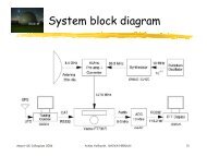
3.8 Transmitter
Fig. 12 shows a block diagram of a typical QPSK transmitter. The nibbler partitions
Pulse
Shaping
Filter
bitstream
input
Nibbler
Carrier
Oscillator
QPSK
output
- ð/
2
Phase
Shifter
Pulse
Shaping
Filter
Figure 12: QPSK Transmitter
the continuous input bitstream into dibits, and routes one bit to the in-phase branch
of the modulator, and the other bit to the quadrature branch of the modulator. The
nibbler also converts each zero to a signal amplitude of -1, and each one to a signal
amplitude of +1.
The pulse shaping filter is a square-root raised-cosine filter that limits the bandwidth
of the QPSK signal. When combined with another square-root raised-cosine
filter at the receiver, the overall response provides a signal with zero ISI.
The carrier oscillator generates cos(2πf c t ), which is phase shifted to sin(2πf c t )
by the− π 2
phase shifter, providing a quadrature carrier to the mixers.
The mixers modulate the in-phase and quadrature carriers with the filtered baseband
signals. The output of both mixers is a BPSK signal. The summer adds the
outputs of the two mixers together to produce QPSK.
3.9 Receiver
All digital receivers must, in general, perform three tasks: estimate the carrier phase
(and frequency), recover the symbol timing and estimate the most likely value of the
received symbol. In order to understand the importance of these tasks, we return to
the expression for a phase modulated signal:
S(t )= √ E s cos(2πf c t+ θ(t )), (5)
15

where E s is the (constant) amplitude of the modulated carrier, f c is the carrier
frequency, θ(t ) is the time varying phase modulation, with the initial phase of the
carrier assumed to be zero for convenience.
In the case of QPSK, θ(t ) ∈ {± π 4 ,± 3π 4
}, and changes (at most) once per symbol.
This is still true when we introduce pulse shaping filters to control signal bandwidth,
though the filters do cause the trajectories between constellation points to differ
from those of the unfiltered case. Using a QPSK signal as an example, we will now
investigate each of the three major tasks the receiver must perform.
3.9.1 Synchronous Down Conversion
The first task of the receiver is to down-convert, or heterodyne, the passband modulation
from the carrier frequency to baseband (DC). In order to do this, the receiver
must know the correct frequency and phase of the carrier. If the frequency and
phase of the local oscillator (LO) in the receiver are precisely matched to those of the
transmitter, the baseband modulation can be recovered. To illustrate this, suppose
the transmitted QPSK signal is S(t ), given in (5),and the complex LO of the receiver
is X (t ):
X (t )= √ E s e −j 2πf c t = √ E s cos(2πf c t )− j √ E s sin(2πf c t ).
When we mix the received QPSK signal with the receiver LO, we get a complex baseband
signal, R(t ):
R(t )= √ E s cos(2πf c t+ θ(t ))·√E
s e −j 2πf c t ,
which simplifies to in-phase (real), R I (t ), and quadrature (imaginary), R Q (t ), components:
R I (t )
R Q (t )
= E s
2 {cos(2π2f c t+ θ(t ))+cos(θ(t ))},
= E s
2 {−sin(2π2f c t+ θ(t ))−sin(−θ(t ))}.
Lowpass filtering removes the double frequency terms, leaving:
R I (t )
R Q (t )
= E s
cos(θ(t )),
2
= E s
sin(θ(t )).
2
R I (t ) and R Q (t ) are the projections of θ(t ), our phase modulation, onto the real and
imaginary axes, respectively. We can recover θ(t ) by noting: sin(x)/cos(x)=tan(x),
and: arctan(tan(x))= x. This leads to:
θ(t )=arctan(R Q (t )/R I (t )),
which is the information-bearing phase modulation placed onto the carrier at the
transmitter. For BPSK, we could uniquely identify the transmitted symbol with only
one projection, but for QPSK, we need both projections in order to identify the transmitted
symbol.
16

3.9.2 Why Asynchronous Down Conversion Fails
The expressions for R I (t ) and R Q (t ) are only valid for a coherent LO; one where the
frequency and phase are precisely matched to the transmitted signal. If these conditions
are not satisfied, then it will not be possible to accurately recover the phase
modulation. To see why this is so, suppose the transmitted signal is given as (5), but
the receiver local oscillator is now:
X (t )= √ E s e −j (2πf c t+δ) ,
where δ is a fixed phase offset between the LO and the transmitted carrier. When we
mix the received QPSK signal with the LO, we obtain:
which simplifies to:
R I (t )
R Q (t )
R(t )= √ E s cos(2πf c t+ θ(t ))·√E
s e −j (2πf c t+δ) ,
= E s
2 {cos(2π2f c t+ θ(t )+δ)+cos(θ(t )−δ)},
= E s
2 {−sin(2π2f c t+ θ(t )+δ)−sin(δ−θ(t ))}.
After lowpass filtering and further simplification, we end up with:
R I (t )
R Q (t )
= E s
cos(θ(t )−δ),
2
= E s
sin(θ(t )−δ).
2
These are not the desired projections of the baseband modulation. The phase offset
between the carriers of the transmitter and the receiver has manifested itself as a
constant phase offset in the recovered baseband signal. This shows up in the constellation
diagram of the receiver as a constant angular offset of the entire constellation.
If there is a frequency offset between the LO and the transmitted carrier, the
situation is worse still. Suppose the LO is:
X (t )= √ E s e −j 2πf x t ,
where f x is the LO frequency, which is different from the true carrier frequency.
When we mix the received QPSK signal with the LO, we obtain:
which simplifies to:
R(t )= √ E s cos(2πf c t+ θ(t ))·√E
s e −j 2πf xt ,
R I (t )
R Q (t )
= E s
2 {cos(2π[f c + f x ]t+ θ(t ))+cos(2π[f c − f x ]t+ θ(t ))},
= E s
2 {−sin(2π[f c + f x ]t + θ(t ))−sin(2π[f x − f c ]t− θ(t ))}.
17

After lowpass filtering and further simplification, we end up with:
R I (t )
R Q (t )
= E s
2 cos(2π[f c − f x ]t+ θ(t )),
= E s
2 sin(2π[f c − f x ]t+ θ(t )).
The frequency offset between the carriers of the transmitter and the receiver has
manifested itself as a frequency offset in the recovered baseband signal. If we examine
the constellation diagram of a baseband signal that has a constant frequency
offset, the entire constellation will rotate at a rate equal to the frequency offset.
Referring to Fig. 9, the symbol decision regions for QPSK are simply the four
quadrants. If a phase or frequency offset causes the constellation points to rotate
off of their nominal positions, the receiver may make errors in deciding which symbol
was received. Thus, the receiver must correctly estimate the transmitted carrier
phase and frequency.
3.9.3 Symbol Timing Recovery
Assuming the receiver has successfully down converted the modulation from passband
to baseband, the next task the receiver must perform is symbol timing recovery.
Each received symbol must be sampled at the proper time in order to obtain the
best immunity from noise. The receiver must sample the symbol at the point where
the ‘eye’ of the eye diagram (see Fig. 7) is open the widest.
When sampling at the correct time, the receiver need only decide whether the
value of the received signal represents a ‘0’ or a ‘1’. In the case of QPSK, we have both
an in-phase and quadrature component to the received symbol, and will thus recover
two bits for each symbol. If we sample the symbol at any point other than
where the eye is at its maximal opening, our decision will be degraded by intersymbol
interference (ISI). With Nyquist pulse shaping, ISI is only zero at one instant
in each symbol interval.
3.9.4 Symbol Demodulation
Once the receiver has identified the correct symbol timing, it must sample each symbol
and estimate the most likely value of the transmitted symbol. The receiver may
produce either a hard output, consisting of two bits for each symbol, or a soft output,
consisting of a quantized estimate of the value of each symbol. For the symbol
mapping given in Table 1, the receiver can produce a hard output by assigning the
sign of the in-phase sample to the first bit of each dibit, and the sign of the quadrature
sample to the second bit of each dibit. The receiver produces a soft output by
quantizing the amplitudes of the in-phase and quadrature samples of each symbol.
3.9.5 Phase Ambiguity
We assume the receiver LO phase is perfectly matched to that of the transmitted
QPSK. However, most phase estimators leave a degree of ambiguity in their estimate.
18

Most commonly, the phase estimator produces a result which may be wrong by a
factor of an integer multiple of π 2
radians. When the carrier phase estimate is off
by this factor, the demodulated bits will be wrong, because the receiver is, in effect,
using a different symbol mapping than the transmitter. In general, a fixed framesync
pattern is sent by the transmitter to resolve any phase ambiguity at the receiver.
3.9.6 Block Diagram
Fig. 13 shows a block diagram of a typical QPSK receiver. The input QPSK signal is
Pulse
Shaping
Filter
QPSK
input
- ð/
2
Phase
Shifter
Carrier
Oscillator
Estimate
Carrier
Phase
Recover
Symbol
Timing
Estimate
Symbol
Value
bitstream
output
Pulse
Shaping
Filter
Figure 13: QPSK Receiver
mixed with a quadrature local oscillator, which heterodynes the modulation from
the carrier frequency to baseband. Since QPSK requires a coherent receiver, the carrier
phase of the LO must be phase synchronized to the received QPSK.
The pulse shaping filter is a lowpass square-root raised-cosine filter that removes
the double-frequency term from the down-converted quadrature baseband signal.
This filter also completes the Nyquist pulse shaping of the signal, resulting in zero
ISI at the optimal sampling time.
The filtered baseband signal feeds a carrier phase estimator that adjusts the local
oscillator phase, forcing it into phase synchronization with the received QPSK signal.
The carrier phase estimator and its associated connection to the LO is typically the
most challenging portion of the receiver design.
The filtered baseband signal also feeds a symbol timing recovery block. This
block determines the optimal symbol timing, and takes a sample of the signal when
the eye of the eye diagram is at its widest opening. This too, is often a challenging
portion of the receiver design.
The last block of the receiver takes an optimally-timed sample of the filtered
baseband signal and forms an estimate of the transmitted symbol. This estimate
is then converted to a dibit and supplied as the output bitstream.
19

4 DPSK
Thus far, we have only considered the possibility of a coherent demodulator for receiving
PSK. A coherent demodulator requires the receiver local oscillator to have its
carrier phase and frequency precisely matched to the transmitted carrier. However,
if we are willing to sacrifice some bit-error-rate performance in exchange for a reduction
in receiver complexity, there is an alternative to the coherent demodulator,
and this is the motivation for differential phase shift keying (DPSK).
Instead of creating an independent phase-coherent local oscillator, we can use
the PSK signal itself as the local oscillator. To do this, we delay the received PSK
signal by exactly one symbol, then mix this delayed signal with the incoming PSK.
This technique is called intermediate frequency (IF) differential demodulation. We
previously defined a PSK signal in (5). If we delay this PSK signal by one symbol, the
value of t becomes (t − T ), where T is the duration of one symbol. If we mix the
received PSK signal with a one-symbol delayed copy of itself, we obtain:
R(t ) = √ E s cos(2πf c t+ θ(t ))·√E
s cos(2πf c (t− T )+θ(t− T ))
= E s
2 {cos(2π2f c t− 2πf c T + θ(t )+θ(t− T ))+cos(2πf c T + θ(t )−θ(t− T ))}.
After lowpass filtering, we have:
R(t )=cos(2πf c T + θ(t )−θ(t− T )).
The term, 2πf c T is a constant, and under certain conditions, may disappear
completely. The phase angle of the present symbol is θ(t ), and the phase angle of
the previous symbol is θ(t− T ). Therefore, the term θ(t )−θ(t− T ) is simply the angular
difference between the present and previous symbols. Thus, by mixing a PSK
signal with a one-symbol delayed copy of itself, we obtain a signal that tells us the
phase difference between the present symbol and the previous symbol.
Another possibility is to use an asynchronous local oscillator to down convert
the PSK from the carrier frequency to baseband, then differentially decode the baseband
signal. This technique is called baseband differential demodulation. Suppose
our PSK signal, S(t ), is (5), and our local oscillator is:
X (t )= √ E s e −j (2πf x t+δ) ,
where f x is the frequency of the LO, and δ is some arbitrary phase. The output of the
down converter will be:
which simplifies to:
R(t )= √ E s cos(2πf c t+ θ(t ))·√E
s e −j (2πf x t+δ) ,
R I (t )
R Q (t )
= E s
2 {cos(2π[f c + f x ]t + θ(t )+δ)+cos(2π[f c − f x ]t+ θ(t )−δ)},
= E s
2 {−sin(2π[f c + f x ]t+ θ(t )+δ)−sin(2π[f x − f c ]t− θ(t )+δ)}.
20

After lowpass filtering and further simplification, we have:
R I (t )
R Q (t )
= E s
2 cos(2π[f c − f x ]t+ θ(t )−δ),
= E s
2 sin(2π[f c − f x ]t + θ(t )−δ).
Next, we calculate arctan(R Q (t )/R I (t )) to extract ̸ R(t ), the argument of the filtered
baseband signal. Finally, we subtract a one-symbol delayed version of ̸ R(t ) from
itself to form ̸ R(t )−̸ R(t− T ). The result is:
2π[f c − f x ]t+ θ(t )−δ−2π[f c − f x ](t− T )−θ(t − T )+δ.
If f x ≈ f c , then the term [f c − f x ] is very small, and can be considered nearly zero over
a one symbol interval. With this approximation, we are left with θ(t )−θ(t − T ), the
phase difference between the present symbol and the previous symbol
Of course, both of these differential receivers are only able to determine the
phase difference between symbols, not the absolute phase of a given symbol. Therefore,
at the transmitter, we must encode our information as a phase difference, rather
than as an absolute phase. To do this, we will assign a phase difference, ∆θ, to
each symbol. Table 2 lists one possible symbol mapping for differential QPSK. To
dibit ∆θ(t )
00 0
01 + π 2
10 − π 2
11 π
Table 2: Differential QPSK Symbol Map
encode the symbols, the transmitter starts with the initial phase value, θ(t = 0),
which may be set to zero for convenience. Then the transmitter follows the rule:
θ(n)=θ(n− 1)+∆θ n , where n is the symbol number, and∆θ n is the value from Table
2 corresponding to the nth symbol. The remainder of the transmitter is identical
to an ordinary QPSK transmitter.
With differential PSK, the receiver does not need a phase-coherent local oscillator.
This leads to a vastly simpler receiver design than that required by PSK. However,
differential PSK suffers from degraded bit-error-rate performance, since the
amount of noise in the received signal is effectively doubled, due to mixing a noisy
signal with a noisy signal instead of a clean local oscillator.
Although the example presented above is differential QPSK (DQPSK), M-ary DPSK
is possible for any value of M, with DBPSK and DQPSK being the most common.
DQPSK can be further modified to obtain π/4-DQPSK, perhaps the most versatile
member of the DPSK family.
21

5 π/4-DQPSK
π/4-DQPSK is a variation of DQPSK, and as such, has four possible symbols. Standard
QPSK maps each of the four symbols to a unique phase angle in an absolute
manner. In other words, the symbol S 00 always maps to θ(t )=+ 3π 4
. π/4-DQPSK uses
differential encoding; therefore, the mapping between symbols and phase angles is
no longer absolute. We begin our study of π/4-DQPSK by exploring the mapping
between symbols and phase angles.
5.1 Symbol Mapping
Consider the symbol mapping of Table 3. Although this table looks similar to the
symbol
∆θ
00 − 3π 4
3π
01
4
10 − π 4
11
π
4
Table 3: π/4-DQPSK Symbol Map
one for QPSK, the value retrieved from this table is the phase increment,∆θ, instead
of the phase angle, θ. At the start of each symbol interval, we use ∆θ to compute θ
according to:
θ new = θ old +∆θ,
then we use θ to shift the phase of the carrier according to:
S(t )= √ E s cos(2πf c t+ θ(t )).
Since ∆θ∈{± π 4 ,± 3π 4
}, each successive symbol will advance the carrier phase by
an odd integer multiple of π 4
. Assuming the initial phase shift at time t = 0 is zero,
the possible phase angles of π/4-DQPSK are {0, π 4 , π 2 , 3π 4 ,π, 5π 4 , 3π 2 , 7π 4 }.
For π/4-DQPSK, we create a baseband signal by using the symbol mapping provided
in Table 3. We first map each dibit to a phase increment,∆θ. Next, we add each
phase increment to the previous phase, θ, reducing the result modulo 2π as necessary.
The result is a sequence of phase angles, which we use to create a complex
baseband signal as:
M(t )= e +j θ(t ) ,
where θ(t ) is one of the eight possible phase angles listed above. This completes the
mapping of dibits to the eight constellation points.
5.2 Constellation
π/4-DQPSK has an eight point constellation, as shown in Fig. 14. Although this constellation
consists of the same eight points as that of 8-PSK, π/4-DQPSK and 8-PSK
22

Imaginary
Real
Figure 14: π/4-DQPSK Constellation Diagram
23

are very different forms of PSK. The π/4-DQPSK constellation consists of two fourpoint
subsets that are offset by π 4
radians from each other. Fig. 14 shows one of these
subsets in dark gray, and the other in light gray.
Since we are always adding an odd multiple of π 4
radians to the phase, the signal
must alternate between these two four-point subsets every symbol. This means, at
each symbol transition, the signal must move from a dark gray point to a light gray
point, or from light gray point to a dark gray point. Moving from a light gray point to
a light gray point, or from a dark gray point to a dark gray point, is forbidden.
5.3 Transition Diagram
Fig. 15 shows the transition diagram for π/4-DQPSK.
1.5
1
0.5
imaginary
0
−0.5
−1
−1.5
−1.5 −1 −0.5 0 0.5 1 1.5
real
Figure 15: π/4-DQPSK Transition Diagram
At each of the eight points in the constellation, shown as black circles, there are
four allowable transitions to the other points in the constellation, shown as thick
black lines. Each transition corresponds to one of the four possible symbol values.
None of the transitions pass through the origin. This helps make the signal envelope
more nearly constant than that of QPSK. Additionally, all eight constellation points
are on the unit circle. This means they all have the same total energy.
As was the case with QPSK, we must filter the baseband signal with a raisedcosine
filter to control the bandwidth. This is done in exactly the same manner
24

as it was for QPSK, with both the I and Q components of the baseband signal being
filtered with a raised-cosine filter. When the baseband signal is filtered with a
raised-cosine pulse shaping filter, the transitions become those shown in light gray
in Fig. 15.
5.4 Eye Diagram
When we view either the in-phase or quadrature component of the baseband signal
transitions versus time, the result is the eye diagram shown in Fig. 16. The eye al-
1.5
1
0.5
relative amplitude
0
−0.5
−1
−1.5
0.5 0 0.5 0 0.5
symbol timing
Figure 16: π/4-DQPSK Eye Diagram
ternates between two levels and three levels at every symbol. This is quite different
from the eye diagram of QPSK, and is due to the alternating subsets of the constellation.
Fig. 14 helps to visualize the projections of the constellation points onto the real
or imaginary axis. The light gray subset of the constellation will project to the two
2
points: ±
2
The dark gray subset of the constellation will project to three points:
0, ±1. Therefore, as the signal alternates between these two subsets, the eye will
alternate between two levels and three levels at every symbol, as shown in Fig. 16.
5.5 Transmitter
Fig. 17 shows a block diagram of a π/4-DQPSK transmitter. The thin lines of Fig. 17
show real signals, and the thick lines show complex signals.
The nibbler partitions the continuous input bitstream into dibits, then supplies
these dibits to the symbol mapper. The symbol mapper maps dibits to points in the
π/4-DQPSK constellation. It does this by looking up the value of ∆θ (from Table 3)
25

input
bitstream
Nibbler
Symbol
Mapper
Shaping
Filter
Carrier
Heterodyne
dqpsk
output
Figure 17: π/4-DQPSK Transmitter
that corresponds to the dibit, then adding this value of ∆θ to the previous value of
θ. We assume the value of θ at time t = 0 is zero, though it can be set to any integer
multiple of π 4
if desired.
Once the symbol mapper has determined the new value of θ, it creates a complex
baseband symbol corresponding to this phase angle. Table 4 lists the real and
imaginary values of the baseband symbol for all possible values of θ.
θ real imaginary
0 +1 0
π
4
+ 2
2
π
+
3π
4
− 2
2
+
2
2
2
0 +1
π -1 0
2
2
5π
4
− 2
2
− 2
2
3π
2
0 -1
7π
4
+
2
2
−
2
2
Table 4: π/4-DQPSK Symbol Table
The symbol mapper then passes the real and imaginary values of each symbol
to the pulse shaping filter. As was the case for QPSK, the pulse shaping filter is a
square-root raised-cosine filter that limits the bandwidth of the signal. Finally, a
quadrature carrier oscillator heterodynes the modulation from baseband to the carrier
frequency.
5.6 Receiver
Although π/4-DQPSK may be demodulated several different ways, the baseband differential
receiver is the easiest to implement in a sampled signal environment. The
baseband differential receiver uses an asynchronous local oscillator to down convert
the π/4-DQPSK from the carrier frequency to baseband, then differentially decodes
the baseband signal. In the section on differential PSK, we showed the argument of
the baseband signal to be:
̸ R(t )=2π[f c − f x ]t+ θ(t )−δ,
where f c is the π/4-DQPSK carrier frequency, f x is the local oscillator frequency, θ(t )
is the phase modulation, and δ is the arbitrary phase of the local oscillator. If we
26

subtract a one-symbol delayed version of this signal from itself, we obtain:
2π[f c − f x ]t+ θ(t )−δ−2π[f c − f x ](t− T )−θ(t − T )+δ.
If the local oscillator frequency is close to the π/4-DQPSK carrier frequency, then the
term [f c − f x ] is essentially zero over one symbol, and the baseband differential signal
is approximately: θ(t )−θ(t − T ), the phase difference between the present symbol
and the previous symbol
Fig. 18 shows a block diagram of the baseband differential receiver. The local
Pulse
Shaping
Filter
arctan
One
Symbol
Delay
-
+
Symbol
Timing
Recovery
Asynchronous
Quadrature
Oscillator
Figure 18: π/4-DQPSK Baseband Differential Receiver
oscillator generates a quadrature carrier that is close to the frequency of the π/4-
DQPSK carrier, but having an arbitrary phase offset. The receiver mixes the asynchronous
LO with the received π/4-DQPSK, to heterodyne the modulation to baseband.
The baseband signal is complex, as indicated by the thick line in Fig. 18. A
square-root raised-cosine lowpass filter removes mixer products from the complex
baseband signal, and also completes the Nyquist pulse shaping.
The output of the pulse shaping filter is processed by an arctangent function to
recover the argument, or angle, of the signal. Next, the receiver places the argument
of the baseband into a one-symbol delay line, then subtracts the output of the delay
line from the input of the delay line. The resulting signal is the difference between
the phase of the present and previous symbols. This phase difference is fed to the
symbol timing recovery block for final demodulation.
5.7 Symbol Timing Recovery
The symbol timing recovery function must estimate the symbol timing; that is, it
must locate the symbol boundaries. Once the symbol timing has been established,
the receiver must sample the signal, then estimate the most likely transmitted symbol,
based on this sample.
The input signal presented to the symbol timing recovery mechanism is ∆θ,
the phase difference between the present sample and the sample one symbol ago.
At the ideal sampling times, ∆θ will converge to one of the four possible values:
π
4 , 3π 4 , 5π 4 , 7π 4
. At all other times, ∆θ diverges from these four values and takes on
many values in the range from zero to 2π. This observation is the key to determining
the symbol timing.
27

Since the filtered baseband signal has a Nyquist pulse shape, θ(t ) will have zero
ISI at one point in each symbol. Likewise,∆θ will also exhibit zero ISI at one point in
each symbol, since it is, by definition, the difference between θ(t ) over exactly one
symbol. At all times other than the ideal sampling time,∆θ will be corrupted by ISI.
We can use this fact to determine the symbol timing.
In many systems, symbol timing recovery is accomplished by inserting a fixed
synchronization pattern into the modulation, then searching for this pattern at the
receiver. This makes symbol timing recovery easy, at the expense of consuming
bandwidth that could be used to carry information.
In addition to determining the correct symbol timing, the receiver must also estimate
the transmitted symbol value that the received signal represents. Since ∆θ
should ideally be± π 4 or± 3π 4
, the decision regions for the received symbols are simply
the four quadrants of complex signal space, and the decision boundaries are the
real and imaginary axes.
5.8 Bit Error Rate Performance
The theoretical bit error rate performance of π/4-DQPSK on a static AWGN channel
is given by:
P b = e −2 E b ∞∑
N 0 { ( 2−1) i I i ( 2 E b
)− 1 N 0 2 I 0( 2 E b
)}.
N 0
This is plotted for E b
N 0
i=0
from 0 dB to 12 dB in Fig. 19. The solid black curve is π/4-
π/4−DQPSK
QPSK
10 −1 E b
/N 0
(dB)
10 −2
bit error rate
10 −3
10 −4
10 −5
10 −6
0 2 4 6 8 10 12
Figure 19: π/4-DQPSK BER on Static AWGN Channel
DQPSK, while the light gray curve is conventional QPSK. As expected, π/4-DQPSK
28

performs about 2 to 3 dB worse than QPSK on an AWGN channel. However, on fading
channels, π/4-DQPSK may perform better than QPSK.
References
[1] Sandeep Chennakeshu, Gary J. Saulnier, “Differential Detection of π 4 -Shifted-
DQPSK for Digital Cellular Radio”, IEEE Trans. Veh. Technol., vol. 42, no. 1, pp.
46-57, Feb. 1993
[2] Kamilo Feher, “Modems for Emerging Digital Cellular-Mobile Radio System”,
IEEE Trans. Veh. Technol., vol. 40, no. 2, pp. 355-365, May 1991.
[3] Steven H. Goode, Hentry L. Kazecki, Donald W. Dennis, “A Comparison of
Limiter-Discriminator, Delay and Coherent Detection for π 4
QPSK”, Proc. IEEE
Veh. Technol. Conf., Orlando, FL, pp. 687-694, May 1990.
[4] Chia-Liang Liu, Kamilo Feher, “Noncoherent Detection of π 4
-QPSK in a CCI-
AWGN Combined Interference Environment” Proc. IEEE Veh. Technol. Conf., pp.
83-94, San Francisco, CA, May 1989.
[5] John G. Proakis, Digital Communications (4th Edition), McGraw-Hill, 2000.
[6] Bernard Sklar, Digital Communications: Fundamentals and Applications (2nd
Edition), Prentice Hall, 2001.
[7] Nelson R. Sollenberger, Justin C. I. Chuang, “Low-Overhead Symbol Timing and
Carrier Recovery for TDMA Portable Radio Systems”, IEEE Trans. Commun., vol.
38, no. 10, pp. 1886-1892, October 1990.
29