Technical Guidance For Deriving Environmental ... - Oekotoxzentrum

Technical Report - 2011 - 055 

Common Implementation Strategy 

for the Water Framework Directive (2000/60/EC) 

Guidance Document No. 27 

Technical Guidance For Deriving 

Environmental Quality Standards

Europe Direct is a service to help you find answers 

to your questions about the European Union 

New freephone number: 

00 800 6 7 8 9 10 11 

A great deal of additional information on the European Union is available on the Internet. 

It can be accessed through the Europa server (http://ec.europa.eu). 

ISBN : 978-92-79-16228-2 

DOI : 10.2779/43816 

© European Communities, 2011 

Reproduction is authorised provided the source is acknowledged. 

Disclaimer: 

This technical document has been developed through a collaborative programme involving the European Commission, 

all the Member States, the Accession Countries, Norway and other stakeholders and Non-Governmental Organisations. 

The document should be regarded as presenting an informal consensus position on best practice agreed by all partners. 

However, the document does not necessarily represent the official, formal position of any of the partners. Hence, the 

views expressed in the document do not necessarily represent the views of the European Commission.

Common Implementation Strategy 

for the Water Framework Directive (2000/60/EC) 

Guidance Document No. 27 

Technical Guidance For Deriving 

Environmental Quality Standards

FOREWORD 

The EU Member States, Norway, and the European Commission in 2000 have jointly developed a 

common strategy for implementing Directive 2000/60/EC establishing a framework for Community 

action in the field of water policy (the Water Framework Directive). The main aim of this strategy is 

to allow a coherent and harmonious implementation of the Directive. Focus is on methodological 

questions related to a common understanding of the technical and scientific implications of the 

Water Framework Directive. In particular, one of the objectives of the strategy is the development 

of non-legally binding and practical Guidance Documents on various technical issues of the 

Directive. These Guidance Documents are targeted to those experts who are directly or indirectly 

implementing the Water Framework Directive in river basins. The structure, presentation and 

terminology are therefore adapted to the needs of these experts and formal, legalistic language is 

avoided wherever possible. 

Under the WFD Common Implementation Strategy, an Expert-Group (EG) on Environmental 

Quality Standards (EQS) was initiated in 2007 to produce guidance on establishment of the EQSs 

in the field of water policy. This activity was led by UK and the Joint Research Centre and 

supported by the Working Group E (WG-E). The Working Group E is chaired by the Commission 

and consists of experts from Member States, EFTA countries, candidate countries and more than 

25 European umbrella organisations representing a wide range of interests (industry, agriculture, 

water, environment, etc.). 

The enclosed Technical Guidance has been developed to support the derivation of EQSs for 

priority substances and for river-basin-specific pollutants that need to be regulated by Member 

States according to the provisions of the WFD. The Commission intends to use the Technical 

Guidance to derive the EQSs for newly identified priority substances and to review the EQSs for 

existing substances. 

Article 16 of the Water Framework Directive (WFD, 2000/60/EC) requires the Commission to 

identify priority substances among those presenting significant risk to or via the aquatic 

environment, and to set EU Environmental Quality Standards (EQSs) for those substances in 

water, sediment and/or biota. In 2001 a first list of 33 priority substances was adopted (Decision 

2455/2001) and in 2008 the EQSs for those substances were established (Directive 2008/105/EC 

or EQS Directive, EQSD). The WFD Article 16 requires the Commission to review periodically the 

list of priority substances. Article 8 of the EQSD requires the Commission to finalise its next review 

by 2011, accompanying its conclusion, where appropriate, with proposals to identify new priority 

substances and to set EQSs for them in water, sediment and/or biota. 

The Scientific Committee on Health and Environmental Risks (SCHER) adopted its opinion on 

Technical Guidance for Deriving Environmental Quality Standards in October 2010 1 . The Water 

Directors endorsed the Guidance during their informal meeting under the Hungarian Presidency in 

Budapest (26-27 May 2011). 

This Guidance Document is a living document that will need continuous input and improvements 

as application and experience build up in all countries of the European Union and beyond. The 

Water Directors agreed to make publicly available the Guidance in its current form in order to 

present it to a wider public as a basis for carrying forward ongoing implementation work. 

The Water Directors would like to thank the leaders of the activity and the members of the Working 

Group E for preparing this high quality document. The Water Directors also commit themselves to 

assess and decide upon the necessity for reviewing this document in the light of scientific and 

technical progress and experiences gained in implementing the Water Framework Directive and 

Environmental Quality Standards Directive. 

1 http://ec.europa.eu/health/scientific_committees/environmental_risks/docs/scher_o_127.pdf

Guidance Document No: 27 

Technical Guidance For Deriving Environmental Quality Standards 

CONTENTS 

1. INTRODUCTION.................................................................................................................................................. 9 

1.1 Environmental Quality Standards (EQSs) under the Water Framework Directive........................................ 9 

1.2 Scope of the guidance .................................................................................................................................... 10 

1.3 Links to chemical risk assessment ................................................................................................................. 11 

1.4 Structure of guidance ..................................................................................................................................... 12 

2. GENERIC ISSUES ................................................................................................................................................ 12 

2.1 Use of EQSs in waterbody classification ....................................................................................................... 12 

2.2 Overview of the steps involved in deriving an EQS ...................................................................................... 13 

2.3 Receptors and compartments at risk .............................................................................................................. 13 

2.4 Identifying the assessments to be performed (receptors at risk) .................................................................... 15 

2.4.1 Water column ..................................................................................................................................... 16 

2.4.2 Sediments............................................................................................................................................ 16 

2.4.3 Biota .................................................................................................................................................. 17 

2.5 Selecting an overall standard ......................................................................................................................... 20 

2.6 Data – acquiring, evaluating and selecting data............................................................................................. 21 

2.6.1 Types of data required for deriving QSs............................................................................................. 21 

2.6.2 Quality assessment of data.................................................................................................................. 23 

2.6.3 ‘Critical’ and ‘supporting’ data............................................................................................................. 24 

2.6.4 Data gaps - non testing methods......................................................................................................... 25 

2.7 Calculation of QSs for substances occurring in mixtures .............................................................................. 26 

2.8 Using existing risk assessments ..................................................................................................................... 26 

2.8.1 Risk assessments under Existing Substances Regulations (ESR)....................................................... 26 

2.8.2 Pesticide risk assessments under 91/414/EEC.................................................................................... 27 

2.9 Extrapolation.................................................................................................................................................. 27 

2.9.1 Mode of action.................................................................................................................................... 28 

2.9.2 Field and mesocosm data.................................................................................................................... 28 

2.9.3 Background concentrations................................................................................................................. 29 

2.10 Dealing with metals ....................................................................................................................................... 29 

2.10.1 Why metals are different..................................................................................................................... 29 

2.11 Expression and implementation of EQSs....................................................................................................... 30 

2.11.1 Accounting for exposure duration ...................................................................................................... 30 

2.11.2 Including aspects of water management and monitoring into the final decision about EQSs ............ 30 

2.11.3 Expression of EQSs for water............................................................................................................. 31 

3 STANDARDS TO PROTECT WATER QUALITY ............................................................................................. 33 

3.1 General approach ........................................................................................................................................... 33 

5



3.2 Derivation of QSs for protecting pelagic species........................................................................................... 33 

3.2.1 Relationship between water column QS and MAC-QS...................................................................... 33 

3.2.2 Preparing aquatic toxicity data ........................................................................................................... 34 

3.2.3 Combining data for freshwater and saltwater QS derivation .............................................................. 35 

3.3 Deriving a QS fw, eco ......................................................................................................................................... 36 

3.3.1 Derivation of a QS for the freshwater community (QS fw, eco ) ............................................................. 36 

3.3.2 Derivation of a QS for the saltwater pelagic community (QS sw, eco ) ................................................... 45 

3.4 Deriving a MAC-QS...................................................................................................................................... 49 

3.4.1 Deriving a MAC-QS for the freshwater pelagic community (MAC-QS fw, eco ) ................................... 50 

3.4.2 Derivation of a MAC-QS for the saltwater pelagic community (MAC-QS sw, eco )............................... 52 

3.5 Deriving EQSs for metals .............................................................................................................................. 54 

3.5.1 Metal specific mechanisms of action.................................................................................................. 54 

3.5.2 Generic guidance on setting quality standards for metals in water and sediments ............................. 54 

3.6 Estimating background levels of metals ........................................................................................................ 63 

3.6.1 General comments .............................................................................................................................. 63 

3.6.2 Estimating backgrounds for freshwater .............................................................................................. 64 

3.6.3 Estimating background concentrations for saltwaters......................................................................... 65 

3.7 Data requirements for deriving QSs for metals.............................................................................................. 67 

3.8 Assessing compliance with a water-column EQS for organic compounds .................................................... 69 

3.8.1 Option to translate an EQS for dissolved water into an equivalent EQS for total water and/or 

suspended particulate matter............................................................................................................... 69 

3.9 Deriving quality standards for water abstracted for drinking water (QS dw, hh ) ............................................... 71 

3.9.1 Overview ............................................................................................................................................ 71 

3.9.2 QS dw, hh for drinking-water abstraction ............................................................................................... 72 

4 DERIVATION OF BIOTA STANDARDS ........................................................................................................... 75 

4.1 Introduction.................................................................................................................................................... 75 

4.2 Protection goals.............................................................................................................................................. 75 

4.3 Expression of a biota standard ....................................................................................................................... 76 

4.4 Deriving a biota standard to protect against the secondary poisoning of predators ....................................... 77 

4.4.1 Identifying the critical data................................................................................................................. 77 

4.4.2 Data requirements............................................................................................................................... 78 

4.4.3 Expressing toxicological endpoints as a concentration in food .......................................................... 78 

4.4.4 Extrapolation to derive a QS biota, secpois ................................................................................................ 79 

4.5 Protection of humans against adverse health effects from consuming contaminated fisheries products ....... 82 

4.6 Metals ............................................................................................................................................................ 82 

4.7 Monitoring compliance with biota standards................................................................................................. 83 

4.7.1 Biota monitoring................................................................................................................................. 83 

4.7.2 Converting QSs expressed as biota concentrations into equivalent water concentrations.................. 84 

5. STANDARDS TO PROTECT BENTHIC (SEDIMENT DWELLING) SPECIES.............................................. 93 

5.1 Introduction.................................................................................................................................................... 93 

5.2 Derivation of sediment standards................................................................................................................... 93



5.2.1 Derivation of EQS sediment for the protection of freshwater benthic organisms .................................... 94 

5.2.2 Metals and the need to cope with bioavailability issues ..................................................................... 103 

5.2.3 Dealing with bioaccumulated/biomagnified substances ..................................................................... 104 

5.2.4 Protection of saltwater benthic organisms .......................................................................................... 104 

5.2.5 Derivation of sediment QS for transitional waters.............................................................................. 105 

5.3 Using sediment QS that are subject to high uncertainty ..................................................................... 106 

5.3.1 Overview ............................................................................................................................................ 106 

5.3.2 Assessing the bioavailable fraction..................................................................................................... 108 

6. LIMITATIONS IN EXPERIMENTAL DATA – USE OF NON-TESTING APPROACHES.............................. 111 

6.1 Grouping of substances / category approach.................................................................................................. 112 

6.2 QSARs ........................................................................................................................................................... 113 

6.3 Analogue approach / read-across ................................................................................................................... 115 

7. CALCULATION OF QS FOR SUBSTANCES OCCURRING IN MIXTURES.................................................. 117 

8 REFERENCES....................................................................................................................................................... 119 

APPENDIX 1: DATA COLLECTION, EVALUATION AND SELECTION............................................................ 127 

APPENDIX 2: PROFORMA FOR EQS DATASHEET ............................................................................................. 175 

APPENDIX 3: BIOCONCENTRATION, BIOMAGNIFICATION AND BIOACCUMULATION.......................... 185 

APPENDIX 4: INVESTIGATION OF FURTHER METHODOLOGIES TO IMPROVE THE PROTECTION 

OF PREDATORS AGAINST SECONDARY POISONING RISK ............................................................................ 189 

APPENDIX 5: GLOSSARY........................................................................................................................................ 197 

APPENDIX 6: OVERVIEW OF TEMPORARY STANDARDS FOR EQS DERIVATION..................................... 199 

APPENDIX 7: LEADERS OF THE ACTIVITY / MEMBERS OF THE EXPERT GROUP..................................... 201 

TABLES 

Table 2.1 Essentiality of metals and metalloids to living organisms ........................................................................... 29 

Table 3.1 Summary of MAC-QS recommendation based on relationship with QS for direct ecotoxicity.................. 34 

Table 3.2 Assessment factors to be applied to aquatic toxicity data for deriving a QS fw, eco ........................................ 38 

Table 3.3 Assessment factors to be applied to aquatic toxicity data for deriving a QS sw, eco ....................................... 47 

Table 3.4 Assessment factors to derive a MAC-QS fw, eco ............................................................................................. 50 

Table 3.5 Assessment factors to derive a MAC-QS sw, eco ............................................................................................ 52 

Table 3.6 Example freshwater background concentrations based on river basin and hydrometric area levels 

obtained from different sources ................................................................................................................................... 65 

Table 4.1 Conversion factors for converting NOAELs (dose) from mammalian toxicity studies into NOECs 

(concentration) ............................................................................................................................................................. 79 

Table 4.2 Assessment factors for the extrapolation of mammalian and bird toxicity data into QS biota , secpois (EC, 

2003) ............................................................................................................................................................................ 80 

Table 4.3 Assessment factors for the extrapolation of mammalian and bird toxicity data into QS biota,secpois in a 

refined assessment........................................................................................................................................................ 81 

Table 4.4 Considerations in expressing a biota standard as a concentration in prey or in the water column............... 85 

Table 4.5 Default BMF values for organic substances ................................................................................................ 87 

Table 4.6 Metals and metalloids classified by essentiality to living organisms........................................................... 89 

Table 5.1 Assessment factors applied to spiked sediment tests (ECHA, 2008)........................................................... 96 

Table 5.2 QSPRs for soil and sediment sorption for different classes (Sabljic et al, 1995)......................................... 100 

7



Table 5.3 Assessment factors for derivation of the QS sediment, sw eco based on the lowest available NOEC/EC10 

from long-term tests (ECHA, 2008)............................................................................................................................ 105 

Table 5.4 Interpretation of bioavailability measurements............................................................................................ 108 

Table 5.5 Solubility products of metal sulphides......................................................................................................... 109 

Table 1. Sources and estimation methods to be screened for physicochemical parameters......................................... 129 

Table 2. Overview and default table structure for identity and physicochemical parameters listed for each 

compound..................................................................................................................................................................... 130 

Table 3: Classification of water according to salinity.................................................................................................. 141 

Table 4: Used abbreviations for exposure times. ......................................................................................................... 142 

Table 5. Summary statistics derived from toxicity studies and their use in EQS derivation........................................ 143 

Table 2. Conversion factors from NOAEL into NOEC for several species................................................................. 152 

Table 3. Default BMF values for organic substances................................................................................................... 156 

Table 4: Sources for the retrieval of human toxicological threshold limits. ................................................................ 158 

FIGURES 

Figure 1.1Role of EQSs in waterbody classification ................................................................................................... 9 

Figure 2.1Key steps involved in deriving an EQS ....................................................................................................... 13 

Figure 2.2Receptors for which an assessment may be required................................................................................... 14 

Figure 2.3Overview of assessments needed and selection of an ‘overall’ EQS........................................................... 15 

Figure 3.1 Recommended general scheme for deriving QSs and the consideration of bioavailability and 

background corrections................................................................................................................................................ 56 

Figure 3.2 Distribution of dissolved zinc concentrations in the Mersey hydrometric area (UK)................................. 65 

Figure 3.3 Schematic overview of the derivation of the quality standard for drinking water abstraction from 

surface water (QSdw, hh)............................................................................................................................................. 74 

Figure 4.1 Steps involved in deriving a biota standard ................................................................................................ 76 

Figure 5.1 Overview of process for deriving a sediment standard............................................................................... 94 

Figure 5.2 Process for the derivation of a QSsediment................................................................................................ 101 

Figure 5.3 Tiered assessment framework for sediments .............................................................................................. 107 

Figure 6.1: Application of non-testing methods........................................................................................................... 112 

Figure 6.2.Stepwise procedure for category development ........................................................................................... 113 

Figure 6.3 Stepwise approach to applying QSARs ...................................................................................................... 114 

Figure 6.4. Stepwise procedure for the analogue approach.......................................................................................... 115



1. INTRODUCTION 

1.1 Environmental Quality Standards (EQSs) under the Water Framework 

Directive 

Article 16 of the Water Framework Directive (WFD) (EC 2000) sets out the strategy against 

chemical pollution of surface waterbodies. The chemical status assessment is used 

alongside the ecological status assessment to determine the overall quality of a waterbody. 

Environmental Quality Standards (EQSs) are tools used for assessing the chemical status of 

waterbodies. The EQS Directive (EC 2008a) establishes the maximum acceptable 

concentration and/or annual average concentration for 33 priority substances and 8 other 

pollutants which, if met, allows the chemical status of the waterbody to be described as 

‘good’. 

EQSs for the 33 substances identified by the EU as Priority Substances (PSs) and Priority 

Hazardous Substances (PHSs) are derived at a European level and apply to all Member 

States. They are also referred to as Annex X substances of the WFD. 

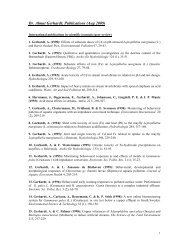
In addition, the WFD (Annex V, section 1.2.6) establishes the principles to be applied by the 

Member States to develop EQSs for Specific Pollutants that are ‘discharged in significant 

quantities’. These are also known as Annex VIII substances of WFD. Compliance with EQSs 

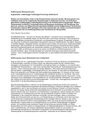
for Specific Pollutants forms part of the assessment of ecological status (Figure 1-1). EQSs 

are therefore key tools in assessing and classifying chemical status and can therefore affect 

the overall classification of a waterbody under the WFD (Figure 1.1). In addition, EQSs will 

be used to set discharge permits to waterbodies, so that chemical emissions do not lead to 

EQS exceedance within the receiving water. 

Biological 

Lowest 

CLASSIFICATION 

Ecology 

High 

Physico-chemical quality 

ECOLOGICAL 

STATUS 

Lowest 

Lowest 

Good 

Mod 

Annex VIII pollutants (EQS) 

Background 

Pass 

Fail 

Pass/fail 

Poor 

Bad 

Chemical 

Annex X + 8 other pollutants 

CHEMICAL 

STATUS 

Pass/fail 

Figure 1.1 

Role of EQSs in waterbody classification 

9



Whilst establishing the principles of EQS derivation, Annex V, Section 1.2.6 of the Water 

Framework Directive does not provide the necessary detail for practitioners to develop EQSs 

in a consistent manner, or cover all the scientific issues that may be encountered. 

In 2005, a technical guidance document was prepared (Lepper, 2005) for the purpose of 

EQS derivation. This covered many of the key technical issues involved in deriving EQSs 

however the science has since moved on requiring the need for an update of the guidance. 

The risk assessment paradigm on which the technical guidance for EQS derivation is based 

(ECHA, 2008) relies on worst-case assumptions. Whilst this is entirely legitimate within a 

tiered assessment framework, to ensure environmental protection, when this paradigm is 

applied to EQS derivation it can lead to unworkable and/or unrealistically low EQS values 

(CSTEE 2 , 2004; Lepper 2005). One of the factors leading to unmanageable water column 

standards is the very low concentrations that arise for some substances with low water 

solubility, or a tendency to bioaccumulate through the food web. If these substances pose a 

significant risk through indirect toxicity (i.e. secondary poisoning resulting from food chain 

transfer), and their analysis is more feasible in other environmental matrices, such as biota 

and/or sediments, then a biota standard or sediment standard may be required alongside, or 

instead of, the water column EQS, as referred to in the EQS Directive 2008/105/EC (Art 3, 

para 2). For this reason, guidance on the derivation of biota and sediment EQSs is required. 

There is also a need for further guidance on setting EQSs for metals in ways that allow 

speciation and bioavailability to be accounted for. Furthermore, we are now in a position to 

refine the guidance for the derivation of water column standards in the light of technical 

advances and experience of EQS setting gained in recent years. These issues are amongst 

those covered in this new guidance. 

1.2 Scope of the guidance 

This guidance document addresses the derivation of environmental quality standards for 

water, sediment and biota. It addresses the need for further guidance highlighted above and 

responds to comments made by the Scientific Committee on Toxicity, Ecotoxicity and the 

Environment (CSTEE, 2004) and by the Scientific Committee on Health and Environmental 

Risks (SCHER) in 2010. It also takes account of the principles highlighted in a SETAC 

(Society for Environmental Toxicology and Chemistry) workshop on environmental standards 

that took place in 2006 (SETAC, 2009) so that the latest scientific thinking on setting and 

implementing environmental standards is reflected. 

This guidance applies to the derivation of EQSs for PSs, PHSs and Specific Pollutants. 

The guidance focuses on the steps required to derive EQSs that comply with the 

requirements of Annex V of the WFD. It assumes that the chemicals for which EQSs are 

required have been identified, i.e. the guidance does not cover chemical prioritisation. 

However, it does address some aspects of the way an EQS is implemented, where this has a 

direct bearing on the way an EQS is derived and expressed, e.g. assessing compliance with 

an EQS. The guidance does not cover issues relating to sampling and chemical analysis: 

these are covered by separate guidance on monitoring (EC, 2010). 

The quantity of data available for deriving an EQS can vary. Where an EQS can be derived 

on the basis of a large dataset there may be only small uncertainties in the final outcome. If, 

however, only a very small dataset is available, the residual uncertainties can be large. 

Uncertainty is accounted for by the use of assessment factors (AFs) but, clearly, there is a 

considerable difference in the robustness and reliability of such EQSs compared to those 

2 Scientific Committee on Toxicity, Ecotoxicity and the Environment



based on extensive data sets, and it may even be inadvisable to implement such EQSs. This 

technical guidance does not recommend when uncertainties are so large that an EQS should 

not be implemented, or used in only an advisory capacity. That decision is for policymakers 

but this could come under review as we gain more experience in setting and using 

environmental standards for the WFD. However, the scientist has an important role in 

advising the policymaker about the major uncertainties and key assumptions involved 

in deriving an EQS. This is particularly important for EQSs which are to be applied 

across Europe (e.g. for Priority Substances or Priority Hazardous Substances). It is 

also important to highlight to the policymaker the practical steps which might be taken to 

reduce uncertainty (e.g. generation of additional ecotoxicity data) and the benefits these 

would have e.g. reducing the size of AFs. The scientist should also advise policymakers 

when uncertainties are small and the resulting EQS is correspondingly robust. With this in 

mind, a proforma technical report is appended (Appendix 2) to prompt the assessor for the 

information that should be reported, including advice to policymakers. 

A further point to add is that confidence about regulatory decisions involving EQSs can also 

be affected by the way in which an EQS is implemented, eg how compliance is assessed. 

Although detailed monitoring guidance lies outside the scope of this guidance, it is useful to 

consider implementation issues during EQS setting. Although the final decision about EQS 

values should reflect the scientific risk, those responsible for EQS derivation are encouraged 

to discuss implications for water management practices with policy makers and those 

responsible for implementing an EQS. These might include, for instance, implications for 

permitting and emission controls, sampling (e.g. whole water vs filtered samples), statistical 

aspects of compliance assessment, availability of suitable analytical methods, the impact of 

residual uncertainty in the EQS and a threshold for the relevance of a specific pollutant for 

which an EQS is needed (e.g. exceedance of 50% of the EQS). 

This guidance is intended for use by environmental scientists with an understanding of the 

principles of risk assessment. A detailed appreciation of the principles and practice of 

environmental chemistry and ecotoxicology is also recommended. Much of this guidance will 

be familiar to those used to dealing with effects assessments under REACH (Registration, 

Evaluation and Authorisation of Chemicals) (Regulation (EC) 1907/2006). 

1.3 Links to chemical risk assessment 

It is important to highlight some conceptual differences between EQS derivation and the 

estimation of a PNEC (Predicted No Effect Concentration) from chemical risk assessment or 

TER (Toxicity Exposure Ratio) for a pesticide. For example: 

 

 

 

 

the concept of an overall threshold (Sections 2.3 and 2.4) that protects all receptors and 

routes is a feature of EQS derivation that does not normally apply in chemical risk 

assessment 

whereas there are opportunities to refine a risk assessment in the light of new data, this 

is often not the case in EQS derivation; although additional data may sometimes be 

voluntarily provided, we cannot usually demand the commissioning of new studies so 

have to utilise what is available to us 

an exceedance of the EQS will not normally trigger a refinement of the standard 

an underlying requirement of the WFD is to protect the most sensitive waters in Europe. 

For metal EQSs, where bioavailability is to be accounted for (Section 2.10) there is 

therefore a requirement to protect a higher proportion of waterbodies than for PNECs 

estimated as part of a risk assessment 

11



 

in EQS derivation, field and mesocosm data have an important role as lines of evidence 

in helping define the standard (through helping reduce uncertainty) but would not be 

regarded as ‘higher tier’ data that would replace laboratory-based ecotoxicity data as 

done in the assessment of the impact of pesticides. 

A PNEC derived as part of a risk assessment will provide a key step in the derivation 

of an EQS and, in some cases, the PNEC from a risk assessment will be identical to 

the EQS. However, for the reasons outlined above, it will not be sufficient to simply 

adopt the PNEC as the EQS as a matter of course. Nevertheless, the process of deriving 

environmental standards is similar to that used in the effects (i.e. hazard) assessment that is 

required for a risk assessment for chemicals. For the purposes of the WFD, short and longterm 

effects are of concern, though greater emphasis is placed on risks from long-term or 

continuous exposure. Authoritative guidance on effects assessment for chemicals has been 

developed, notably the technical guidance developed for industrial chemicals (now under 

REACH (ECHA, 2008)) and pesticides under Directive 91/414/EEC. Annex V of the WFD 

refers directly to the methodology described for the Existing Substances Regulation (ESR) 

(now under REACH). Furthermore, the guidance for undertaking risk assessment of 

pesticides allows for short term impacts and recovery. As far as possible, the technical 

guidance for EQSs described here is consistent with the guidance for effects assessments 

performed for chemical risk assessment under REACH. 

1.4 Structure of guidance 

Generic issues and principles that apply to the derivation of EQSs across all media and 

receptors are outlined in Section 2. The guidance is separated into sections dealing with 

different environmental media, ie derivation of EQSs for the water column are considered in 

Section 3, those for biota in Section 4 and those for sediment in Section 5. Risks from metals 

pose particular challenges and the guidance reflects the latest scientific developments for 

taking account of speciation and bioavailability in deriving thresholds and assessing 

compliance with these EQSs. Detailed guidance for deriving EQSs for metals in water, biota 

and sediment is given in the respective Sections. Recognising the growing importance of 

computational and non-testing methods in the estimation of environmental hazard, guidance 

on the use of such methods when deriving EQSs is given in Section 6. Finally, Section 7 

outlines how to estimate EQSs for mixtures. 

At various points in the guidance, we refer to Appendices and scientific background 

documents to accompany the guidance. These are intended to provide more detailed 

explanations for the technical advice given here. 

2. GENERIC ISSUES 

2.1 Use of EQSs in waterbody classification 

The WFD establishes a framework for protection of all surface waters and groundwaters, with an 

obligation to prevent any deterioration of status, and to achieve good status, as a rule by 2015. The 

overall good status is reached for a certain waterbody if both ecological and chemical status are 

classified as good. 

EQSs established at EU level by the EQS Directive (2008/105/EC) for the 33 priority substances 

and 8 other pollutants are used within the WFD to assess the chemical status of a waterbody. 

Good chemical status is achieved where a surface waterbody complies with all the environmental 

quality standards listed in Part A of Annex I of EQS Directive and applied according with the



requirements set in Part B of Annex I of the same directive. If not, the waterbody shall be recorded 

as failing to achieve good chemical status. 

For Annex VIII substances (Specific Pollutants), each Member State shall establish their EQSs 

according to Annex V, Section 1.2.6 of WFD. Specific Pollutants are supporting parameters for 

biological quality elements, thus they contribute among other parameters to the ecological status 

classification. If the EQSs for these substances are not met, the waterbody can not be classified 

as either ‘Good’ or ‘High’status, even if the biological quality is ‘Good’ or ‘High’ (Figure 1.1). 

2.2 Overview of the steps involved in deriving an EQS 

Figure 2.1 illustrates the key steps that are involved in deriving an EQS, irrespective of the 

compartment or receptor at risk. The key steps are broadly consistent across all media/receptors. 

However, the detail within each step can differ markedly between compartments and receptors. 

Identify receptors and 

compartments at risk 

Identify assessments that need to be undertaken (Section 2.4) 

Collate and quality assess 

data 

Identify physicochemical properties of substances and collect ecotoxicity 

(and possibly computational) data for use as input to standard-setting 

process. Details in Section 2.6 and throughout guidance 

Extrapolation 

Extrapolation to threshold concentration using deterministic or 

probabilistic methods applied to toxicity data from laboratory, 

mesocosms or field studies. Principles outlined in Section 2.8 and 

methods detailed throughout guidance 

Propose EQS 

Propose threshold concentration that applies in water column, sediment 

or biota. Identify key assumptions and uncertainties. Selection of overall 

EQS (Section 2.5) 

Implement EQS 

Design of compliance assessment regime and monitoring requirements 

Figure 2.1 

Key steps involved in deriving an EQS 

2.3 Receptors and compartments at risk 

EQSs should protect freshwater and marine ecosystems from possible adverse effects of 

chemicals as well as human health via drinking water or ingestion of food originating from aquatic 

environments. Several different types of receptor therefore need to be considered, i.e. the pelagic 

and benthic communities in freshwater, brackish or saltwater ecosystems, the top predators of 

these ecosystems and human health. 

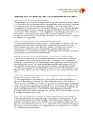
The receptors and media of concern to EQS setting covered in this guidance are illustrated in 

Figure 2.2. 

13



Environmental compartment 

Water Sediment Biota 

Humans Yes No Yes 

(consumption 

of fish 

products) 

Receptor(s) 

at risk 

Figure 2.2 

Sediment 

dwelling biota 

Pelagic 

biota 

Top 

predators 

(birds, 

mammals) 

No Yes No 

Yes No Yes 

(secondary 

poisoning) 

Yes No Yes 

(secondary 

poisoning) 

Receptors for which an assessment may be required 

Yes = potential risks to receptor need to be considered in EQS derivation 

No = risks do not need to be addressed in EQS derivation 

Not all receptors need to be considered for every substance. This depends on the environmental 

fate and behaviour of the substance i.e. if a substance does not bioaccumulate (or doesn’t have 

high intrinsic toxicity), there is no risk of secondary poisoning and so a biota standard is not 

required. However, where a possible risk is identified, quality standards should be derived for that 

receptor (Figure 2.3). Criteria to help identify which of the assessments are needed for a particular 

substance are given in Section 2.4. Where several assessments are performed, the lowest (most 

stringent) of the thresholds will be selected as an ‘overall’ EQS as illustrated in Figure 2.3 and 

detailed in Section 2.5. 

In this way, all relevant protection objectives should be taken into account. Moreover, all direct and 

indirect exposure routes in aquatic systems i.e. exposure in the waterbody via water and sediment 

or via bioaccumulation, as well as possible exposure via drinking water uptake, are accounted for. 

Figure 2.3 presents the routes taken into account for the freshwater compartment, similar routes 

are considered for the saltwater compartment, but indicated with different subscripts (fw is replaced 

by sw in the figure below) See appendix 6 for clarification of the temporary standards used during 

EQS derivation. 

14



* QS dw,hh can only be adopted as the lowest QS water for waters intended for drinking water use 

** unless monitoring in biota is strongly preferred. Under these circumstances, calculate QS biota that is 

equivalent to lowest (i.e. most protective) QS water and select this value as EQS biota 

Figure 2.3 

Overview of assessments needed and selection of an ‘overall’ EQS 

The mode of toxic action for a chemical is not always known but, when carrying out an 

assessment, all relevant modes of toxicity need to be considered. No plausible toxicological hazard 

should be excluded from consideration. Stressors for which an EQS could be derived, but do not 

act by chemical toxicity (e.g. temperature, pH) may require a different approach than that 

described here. Such physical stressors lie outside the scope of this guidance. 

2.4 Identifying the assessments to be performed (receptors at risk) 

According to Article 3 of the EQS Directive, quality standards shall apply to contaminant 

concentrations in water, sediments and/or biota. As illustrated in Figure 2-3, an assessment for 

several compartments is needed when a substance could pose a risk through direct toxicity 

in the water column, to predators through the food chain, or to benthic (sediment-dwelling) 

biota. On the other hand, a QS is not required if a substance will not pose a risk to a 

particular compartment. For instance, a quality standard for sediment is not necessary if the 

substance is unlikely to partition to, or accumulate in, sediment. Similarly, quality standards for 

biota are not required if a substance does not bioaccumulate (or doesn’t have high intrinsic 

15



toxicity), in which case it is reasonable to conclude that there is no risk of secondary poisoning of 

top predators, or to human health from consumption of fishery products. 

The criteria for identifying which assessments are required are outlined below. 

2.4.1 Water column 

An assessment to protect pelagic (i.e. water column) organisms from direct toxicity to chemicals is 

always undertaken. A drinking water threshold is also required for waters used for drinking water 

abstraction. For these waters, existing health-based standards from either the Drinking Water 

Directive 98/83/EC or World Health Organization (WHO) could be used, if available, as the basis 

for the QS derivation, as described in Section 3.9. If no existing standards are available, an 

assessment of risks to human health from drinking water will be required. However, a QS to protect 

waterbodies designated for drinking water abstraction is required only when it is lower (i.e. more 

stringent) than the water column QS to protect aquatic life. A derivation is not required if existing 

drinking water standards are less stringent (i.e. higher) than the water column QS to protect 

aquatic life. 

In the derivation of QSs to protect human health two major exposure routes are considered 

(consumption of fishery products and consumption of drinking water). There may be other routes of 

exposure, such as exposure during recreation (dermal exposure, ingestion of water). These routes 

are of minor importance compared to the other routes considered (see for example Albering et al, 

1999) and are therefore not considered in this guidance. 

2.4.1.1 EQSs for transitional waters 

Separate EQSs are recommended for freshwaters and saltwaters. However, transitional (e.g. 

estuarine) waters are intermediate in salinity which can vary on a diurnal cycle. For waters with a 

low salinity, supporting communities that are closely related to freshwater ecosystems, the 

freshwater scheme is more appropriate. At salinity levels between 3 and 5‰ there is a minimum 

number of species present and this can be considered as a switch from communities that are 

dominated by freshwater species to communities that are dominated by saltwater species. 

Therefore, EQSs in this document are not reported for ‘transitional ánd marine waters’, but either 

for freshwaters or saltwaters. As a default, we recommend a salinity of 5‰ as the cutoff unless 

other evidence suggests a different cutoff is appropriate for a particular location. For instance, 

Bothnian Sea (inner BalticSea) is a brackish water body that has a salinity of around 5‰, and has, 

so far, been treated as a saltwater system. 

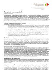
2.4.2 Sediments 

Not all substances require an assessment for a sediment standard. The criteria for triggering an 

assessment are consistent with those under REACH Regulation (EC) No 1907/2006 (ECHA, 2008, 

Chapter R.7b). In general, substances with an organic carbon adsorption coefficient (K oc ) of



Evidence of Sorption Potential 

Log Koc ≥3? 

OR 

Log Kow ≥3? 

OR 

Is there other evidence of accumulation in sediments (e.g. sediment monitoring data)? 

OR 

Is there evidence of high toxicity to benthic organisms? 

YES 

CONDUCT SEDIMENT EQS ASSESSMENT 

NO 

NO ASSESSMENT REQUIRED 

2.4.3 Biota 

The criteria determining whether or not a biota standard is needed are more complex. A standard 

would be required if there was a risk of secondary poisoning of predators (e.g. mammals or birds) 

from eating contaminated prey (QS biota,secpois ), or a risk to humans from eating fishery products 

(QS biota, hh food ). 

The triggers are based on those used to determine whether a secondary poisoning assessment is 

necessary for a substance under REACH Regulation (EC) No 1907/2006 (ECHA, 2008) 3 . The 

triggers for derivation of a QS biota, hh food are dominated by hazard properties whereas a QS biota sec pois 

is triggered by the possibility of accumulation in the food chain in conjunction with hazard 

properties. There are differences between how metals and organic substances are dealt with, and 

these are highlighted below. 

3 The criteria used to determine whether a substance is Persistent, Bioaccumulative and Toxic (PBT) or very 

Persistent and very Bioaccumulative (vPvB) under Annex XIII of REACH are more stringent and not suitable 

for use as a screening decision tree since a substance meeting the PBT/vPvB criteria would require stricter 

management control than standard setting. 

17



2.4.3.1 Protection of predators from secondary poisoning 

(1) Organic substances 

Step 1: Evidence of Bioaccumulation Potential 

Is measured BMF>1 or BCF (BAF) ≥100? 

OR 

If no valid measured BMF or BCF (BAF) is available, is Log Kow ≥ 3 ? 

OR 

Is there other evidence of bioaccumulation potential (e.g. biota monitoring data, structural alerts)? 

PROVIDED THAT there is no mitigating property such as rapid degradation (ready biodegradability 

or hydrolysis half-life



chains, even for inorganic metal forms. It is especially important to look for evidence of organometallic 

species being formed in some compartments, or if the range over which homeostasis 

occurs is relatively small (e.g. selenium). Therefore, a useful first step is to review the information 

available for the metal in question in order to assess whether an in-depth secondary poisoning 

assessment is needed. 

A lack of biomagnification should not be interpreted as lack of exposure or no concern for trophic 

transfer. Even in the absence of biomagnification, aquatic organisms can bioaccumulate relatively 

large amounts of metals and this can become a significant source of dietary metal to their 

predators (U.S. EPA 2007; Reinfelder et al. 1998). 

For metals, a BCF should not be used. This is because the model of hydrophobic partitioning, 

giving a more or less constant ratio C biota /C water with varying external concentration, does not apply 

to metals. For a number of metals an inverse relationship between BCF and external (water-) 

concentration is observed (McGeer et al., 2003). Consequently, BCFs and BAFs are not constant 

with water concentration. Furthermore, some metals are essential for life and many organisms 

possess mechanisms for regulating internal concentrations, especially essential metals such as 

copper and zinc. 

Instead, a case-by-case evaluation of the possibility of dietary toxicity is required: 

 

 

 

 

Information on metal mode of action and homeostatic (internal regulation) controls 

Information on essentiality 

Information on biomagnification (BMF). An example of a study relevant in addressing this 

question is Ikemoto et al (2008a) 

Information on major toxicities i.e. whether main risks are through direct toxicity to pelagic 

organisms or secondary poisoning. With regards to the potential for secondary poisoning the 

assessment of the mode of toxic action in both prey and predator is a key consideration. If 

there is no evidence of biomagnification (i.e. BMF



a substance known or suspected to affect reproduction (Cat. I-III, R-phrases R60, R61, R62, 

R63 or R64) or 

 

 

possible risk of irreversible effects (R68) or 

the potential to bioaccumulate (see protection of top predators) plus danger of serious 

damage to health by prolonged exposure (R48) or harmful/toxic/fatal when swallowed 

(R22/R25/R28). 

Note that applicability of these toxicological triggers should follow from R or H phrases, but 

information obtained from evaluation of toxicological data not necessarily reflected in classification 

and labelling phrases should not be neglected. It may warrant derivation of a risk limit for human 

health based on the consumption of fishery products. 

The H-statements will soon replace the R-phrases in EU chemicals legislation via the 

Classification, Labelling and Packaging Regulation (2008) (EC, 2008). The conversion between H 

and R phrases is provided below. Check the status of the R and H phrases. For those substances 

where R or H phrases have not been harmonised at the EU-level, consultation with (a) human 

toxicological expert(s) is needed. 

R22 

R25 

R28 

R40 

R45 

R46 

R48 

R60 

R61 

R62 

R63 

R64 

R68 

H302: Harmful if swallowed 

H301: Toxic if swallowed 

H300: Fatal if swallowed 

H351: Suspected of causing cancer 

H350: May cause cancer 

H340: May cause genetic effects 

H373: May cause damage to organs through prolonged or repeated exposure 

H360: May damage fertility or the unborn child 

H360: May damage fertility or the unborn child 

H361: Suspected of damaging fertility or the unborn child 

H361: Suspected of damaging fertility or the unborn child 

H362: May cause harm to breast-fed children 

H341: Suspected of causing genetic effects 

2.5 Selecting an overall standard 

Standards for water, sediment and biota are derived independently and they should all be made 

available for possible implementation. Where several assessments are performed for the same 

compartment (e.g. water: protection of pelagic species, protection of human health from drinking 

water; biota: protection of biota from secondary poisoning, protection of human health from 

consuming fisheries products), the lowest standard calculated for the different objectives of 

protection will normally be adopted as the overall quality standard for that compartment. An 

exception will be when the drinking water route results in the lowest (most stringent) QS but a 

waterbody is not designated as a source of drinking water. It is not sufficient to simply report the 

20



‘overall’ EQS; the assessor must make available all the relevant QSs and their derivations. 

Standards for freshwater and saltwaters will be derived independently so the overall EQS saltwater 

may be different to the overall EQS freshwater . 

To select an overall EQS, quality standards will need to be expressed in the same units (i.e. 

mass/volume). This means that biota standards must be ‘back-calculated’ to the corresponding 

water concentration. This is referred to in Figure 2-3 and further guidance is given in Section 2.5.1. 

Finally, sediment QSs are dealt with independently of water column and biota standards. This 

leads to selection of a separate, overall EQS sediment . 

2.5.1 Converting biota standards into an equivalent water concentration 

Procedures for converting biota standards into water column concentrations are given in Section 

4.7.2. It should be noted that the conversion from a biota standard into an equivalent water 

concentration can introduce uncertainty, especially for (a) highly lipophilic substances and (b) 

metals. 

(a) Where it is necessary to convert a biota QS into an equivalent water column concentration 

for a highly lipophilic substance, the uncertainties may be taken into account by performing 

the conversion for extreme BAF values as well as the typical BAF value. If the QS for water 

lies within the range of possible extrapolated values of the QS for biota, when considering 

the uncertainties of the extrapolation, it is not possible to determine with high confidence 

which is the ‘critical’ QS. These should be reported as key uncertainties, outlining the 

implications for implementing an EQS. 

As explained in Section 2.4.3.1, BCF data for metals may be unreliable. Instead, BAF or 

BMF data are preferable. To compare a biota standard with water column standards, refer 

to Section 4.7.1.2. 

(b) For an organic substance, if the log K OW ≥3 criterion is met, but no experimental evidence is 

available on BCF or BMF then the assessor should estimate BCF or BMF from log K OW and 

translate the biota standard to a water concentration for comparison with water column 

standards (Section 4.7.1.2). If the estimated QS for biota is the most stringent (i.e. lowest) 

value, then further investigation to improve BCF and BMF values would be necessary, 

otherwise there is a risk of developing an unrealistically low QS value for water. 

2.6 Data – acquiring, evaluating and selecting data 

Comprehensive and quality assessed data are key inputs to QS derivation. Indeed most of the 

resource required for QS derivation is expended on collecting and assessing data. Appendix 1 

provides detailed guidance on how to locate relevant data, evaluate the data to assess their 

suitability for QS derivation, and select data that will be used to determine a QS. 

A brief summary of the main types of data required for deriving QSs is provided below (Section 

2.6.1), along with details of the quality assessment of data (Section 2.6.2), and the identification of 

‘critical’ and ‘supporting’ data (Section 2.6.3). 

2.6.1 Types of data required for deriving QSs 

2.6.1.1 Data on physical and chemical properties 

Properties which can be very important when interpreting laboratory and field ecotoxicity are water 

solubility, vapour pressure, photolytic and hydrolytic stability, and molecular weight (when 

assessing risks of bioaccumulation). Such data will make it clear when steps to control exposure 

concentrations in ecotoxicity experiments are particularly important. This, in turn, helps assess how 

21



reliable a toxicity study is (Section 2.6.2). In addition, partition coefficients are needed when 

deriving a sediment QS when derived using EqP, to conduct transformation calculations (e.g. from 

mass/volume [mg/L] to mass/mass [mg/kg]). These coefficients (K) include, for example: Koctanolwater 

(K ow ), K suspended particulate matter – water (K susp-water ), K sediment – water (K sed-water ), 

K organic carbon (K oc ). 

2.6.1.2 Ecotoxicological data 

According to Annex V of the WFD, the base set of taxa that should be used in setting quality 

standards for water are algae and/or macrophytes, Daphnia (or representative invertebrate 

organisms for saline waters), and fish in relation to water column standards. For sediment QSs, the 

range of species should be expanded to include benthic species (Section 5). However, for the 

purpose of quality standard setting, the data should not be restricted to this base set. All available 

data for any taxonomic group or species should be considered, provided the data meet 

quality requirements for relevance and reliability (Section 2.6.2). This may include data for 

alien species and even exotic species 5 , although care should be taken with data generated from 

experiments using species from extreme environments (e.g. thermophiles, halophytes). 

If there are indications of endocrine activity (e.g. bioassays), but not studies are available that allow 

assessment of adverse effects through this mechanism, this should be highlighted as an 

uncertainty in the technical report. 

Often, multiple data are available for the same species and endpoint (e.g. several studies 

assessing acute toxicity to Daphnia). Unless there is a clear reason for differences between toxicity 

(e.g. different test conditions, different exposure periods, different life stages or forms of the 

substance tested, like different metal species), any variation in toxicity may simply reflect random 

error and the valid data may be aggregated into a single value for each species and endpoint. 

Detailed guidance on data aggregation is given in Appendix 1 

Finally, using ecotoxicological data to derive QSs for metals requires additional considerations. 

These are dealt with in detail in the relevant sections. 

2.6.1.3 Mammalian toxicity data 

QSs to protect human health utilise information about effects on mammals from oral exposure, 

repeated dose toxicity, carcinogenicity, mutagenicity and effects on reproduction, typically No 

Observable Adverse Effect Level (NOAEL), Acceptable Daily Intake (ADI) and Tolerable Daily 

Intake (TDI) values identified in the human health section of risk assessments performed under the 

REACH regime. Oral Reference Doses (RfD), ADI or TDI values adopted by national or 

international bodies such as the World Health Organization may also be used. For some 

substances, a threshold level cannot be established (e.g. some genotoxic carcinogens). For these, 

risk values corresponding to an additional risk of, e.g., cancer over the whole life of 10 -6 (one 

additional cancer incident in 10 6 persons taking up the substance concerned for 70 years) may be 

used, if available. 

To assess the risk of secondary poisoning of predators, bird and mammal toxicity data are also 

used. Further details are to be found in Appendix 1. 

5 This is because test species not only represent species that occur in European waterbodies but to ensure a 

range of sensitivities is represented in the dataset with the result that any resulting QS is more likely to 

protect the range of species sensitivities found in nature. 

22



2.6.1.4 Data on bioaccumulation 

Data on bioaccumulation (bioconcentration, biomagnification and/or the octanol-water partition 

coefficient (K ow )) are required if a substance has a potential to bioaccumulate (i.e. it exceeds the 

trigger-values given in Section 2.4.4). Where data are available that give different indications of 

bioaccumulation potential, preference should be given to field observations on bioaccumulation 

and biomagnification factors (BAFs, BMFs) or experimentally derived BCFs and BMFs (and TMFs 

– Trophic Magnification Factor), if available. 

Further details on how to obtain and evaluate data on bioaccumulation can be found in Appendix 1. 

2.6.2 Quality assessment of data 

A rigorous assessment of the data is needed to ensure that data are reliable and relevant. This 

will normally entail a review of the original study report, especially for critical data that are likely to 

have a major impact on the QS (Section 2.6.3). 

Reliability refers to the inherent quality of the method used to conduct the test. A reliable 

study requires all relevant details about the test to be described. Relevance means the extent 

to which a test provides useful information about the hazardous properties of a chemical. Only 

reliable, relevant data should be considered valid for use in setting a quality standard. 

2.6.2.1 Reliability 

Guidance on the principles of data validation and the aspects to be considered is given in 

Appendix 1, based on REACH guidance. Data are assigned a score according to the reliability of 

the study. 

Further assessment of data generated or assessed under Community legislation such as 

Regulations (EC) 793/93 and 1488/94 (existing chemicals) or Directives 91/414/EC (plant 

protection products) or 98/8/EC (biocides) is required unless the data published in the risk 

assessment reports under these legal frameworks have already been subjected to data quality 

assurance controls and peer-review. The same applies to peer-reviewed data or guidance values 

(e.g. Tolerable Daily Intakes or Drinking Water values) published by (inter)national organisations 

such as the World Health Organization (WHO), the United Nations Food and Agriculture 

Organization (FAO), the Organisation for Economic Development (OECD) or the OSPAR 

Convention for the Protection of the Marine Environment of the North-East Atlantic; 

Studies on pesticides may be performed on technical material or formulated product. Preference is 

given to data using technical material because toxicity of the active ingredient is less prone to 

modification by other formulation ingredients, but specific guidance on treatment of 

ecotoxicological data for pesticides when formulations have been tested is given in Appendix 1. 

Not all studies on plant protection properties are suitable for EQS derivation because the exposure 

regimes are sometimes very short to simulate specific exposure scenarios (mesocosm studies for 

example). 

Studies that have been performed to ‘Good Laboratory Practice’ (GLP), to international (e.g. 

OECD) test guidelines and submitted under a regulatory regime may be taken at ‘face value’ 

without further review. This is because they have already been reviewed by a competent authority 

and there is a precedent for their acceptability. An exception to this would be if ecotoxicity studies 

submitted as part of a regulatory dossier have been performed in such a way that they might not 

be relevant to QS derivation e.g. unusual exposure regimes or very short test durations. 

Detailed guidance for the selection of data to be used for standard setting is provided in Appendix 

1, but the following principles are highlighted here: 

23



24 

1. Only data that can be considered as valid may be used, irrespective of the source of the 

data. Admissible data are not confined to GLP studies. 

2. Data should be collated in a database with quality scores clearly assigned to each datum. 

Only those considered as valid (see Appendix 1, section "Toxicity data") should be 

used as ‘critical’ data (Section 2.6.3) in deriving an EQS. 

3. If a QS for a particular receptor cannot be derived because the required data are lacking, 

this should be flagged. 

Again, metals data require additional considerations and these are covered in Section 2.10. 

2.6.2.2 Relevance 

A study can be well conducted and fully reported but the test endpoint may have little ecological 

significance. Studies used for EQS derivation should be those where the test endpoint can be 

related to ecologically significant hazards. For practical purposes, this means effects that can be 

linked to population sustainability and particularly: 

a. survivorship of adults 

b. time taken to develop (particularly to reach reproductive age) 

c. reproductive output 

Most standard test methods include one or more of these endpoints. However, the assessor may 

be faced with data from studies describing endpoints that do not include direct measurements of 

survival, development or reproduction but, rather, describe e.g. behavioural effects, anatomical 

differences between control and treatment groups, effects at the tissue or sub-cellular level, such 

as changes in enzyme induction or gene expression. Generally these are unsuitable as the basis 

for EQS derivation. However, some other endpoints are relevant. For example, anatomical 

changes to gonad development that would prevent successful reproduction, or changes in 

behaviour if the effect described would impair competitive fitness may be relevant. Avoidance 

reactions may also be relevant if populations are likely to avoid a contaminated habitat where they 

would normally be present. Further examples are given in Appendix 1 . 

2.6.3 ‘Critical’ and ‘supporting’ data 

Not all data have an equal influence on QS derivation. Critical data are ecotoxicity data (typically 

NOECs/EC10s or LC/EC50) for sensitive species and endpoints that are used as the basis for 

extrapolation and hence determine – or strongly influence - the value of the QS. Section 3 details 

the various approaches for extrapolation in particular deterministic and probabilistic methods. 

Critical data play a key role where a deterministic approach to extrapolation is used (i.e. an AF is 

applied) because the AF is applied to the lowest credible NOEC/EC10 or LC/EC50 (the critical 

datum). If a species sensitivity modelling approach is adopted, a distinction between critical and 

supporting data does not apply. This is because all the data are used in the model extrapolation 

and so, all the data can be regarded as critical (as long as they are reliable and relevant). 

Supporting data are those data that are not described as critical data. They include data that are 

not among the most sensitive species/endpoints, studies that have estimated a non-standard 

summary statistic e.g. a LOEC is reported but no NOEC, field or mesocosm experiments that are 

difficult to interpret, or where a study might be sound but is not fully reported. Supporting data are 

not used directly for QS derivation when using the deterministic approach but can help inform the 

derivation of the QS by, for example, identifying sensitive taxa, determining if freshwater and 

saltwater datasets can be combined for QS derivation, averaging or aggregating the data in order 

to identify the critical data, and selecting an appropriate AF. All reliable and relevant data are used



when deriving a QS using the probabilistic approach, ie SSDs. Experiments that are clearly 

flawed should not be used in any way, even as supporting data. 

It is essential that all available toxicity data, both critical and supporting , are subject to rigorous 

quality assessment and are comprehensively reported as all data may be used, eg in the derivation 

of an SSD, for aggregation of data for the same species and end point and for comparison of fresh 

and saltwater data. Further guidance can be found in Appendix 1. 

2.6.4 Data gaps - non testing methods 

A lack of experimental data can lead to high uncertainty in the derivation process, possibly 

resulting in over-precautionary QSs. Whilst the generation of well-targeted experimental data can 

be critical in helping reduce uncertainty, it can be expensive and time-consuming. Under these 

circumstances there is a useful role for computational methods to fill data gaps, including 

quantitative structure–activity relationships (QSARs) for predicting toxicity and quantitative 

structure-property relationships (QSPRs) for estimating physicochemical properties. ‘Read across’ 

approaches can also be useful to infer the properties of chemicals for which data are absent, 

based on the properties of closely related analogues. Such approaches are now recommended in 

chemical risk assessment (ECHA 2008). Chemical regulation activity and the effort to reduce 

animal testing under REACH may lead to an increased regulatory acceptance of this type of 

information and new tools for deriving non-test data. The use of QSARs to predict toxicity has 

been examined in the following European research projects: 

DEMETRA (Emilio Benfenati: Quantitative Structure-Activity Relationships (QSAR) for Pestide 

Regulatory Purposes; Elsevier 2007, ISBN: 978-0-444-52710-3): Prediction of five ecotoxicological 

endpoints: Acute toxicity trout, daphnia, quail (oral and dietary exposure), and bee 

CAESAR http://www.caesar-project.eu/: Prediction of five toxicological endpoints: 

Bioconcentration factor, skin sensitisation, carcinogenicity, mutagenicity, developmental 

toxicity 

Detailed guidance on non-testing approaches is given in Section 6 but possible applications are 

briefly summarised below. 

2.6.4.1 Predictive models (QSARs, QSPRs) 

The most likely application for computational methods is to fill non-critical data gaps (Section 2.6.3) 

in the dataset for acute aquatic toxicity, especially when a deterministic assessment is to be 

followed. It is vital that computational methods are used within their legitimate operating domains; 

further guidance on QSARs and their use is given in Section 6. 

2.6.4.2 Analogue approaches 

Further non-testing methods include ‘read across’ and ‘category’ approaches. The most likely 

application of read-across is to fill data gaps, when the setting of a QS for mixtures, eg 

polyaromatic hydrocarbons (PAHs) is preferred compared to the QS for individual substances 

(Section 2.6.5). 

Section 6 outlines another approach for inferring the properties, including ecotoxicological 

properties, of substances for which data are lacking. Essentially, it uses a category building 

approach in which chemical analogues are arranged by some physicochemical property (e.g. log 

Kow) and data from close neighbours are used to fill data gaps by interpolation. The approach can 

have value in demonstrating that additional AFs are not justified when using data for one 

substance to derive a QS for another closely related one. However, the following criteria must be 

met: 

25



There is a consistent and reliable trend within a category that is relevant to the endpoint of 

interest (e.g. log K ow increases as ecotoxicity increases) 

 

If toxicity is the endpoint of interest, reliable measured toxicity is needed to identify the most 

sensitive trophic group 

Reliable measured data for the endpoint of interest, allowing interpolation to a value for the 

substance of interest (i.e. where there is a data gap) 

 

QSARs may be used to support read across but cannot be used to replace measured values 

Predictive and analogue methods may be used for generating supporting data but are not 

suitable for predicting toxicity to be used as critical data. Furthermore, the range of 

substances to which these models can be applied is limited to chemicals with certain 

physicochemical and mode of action properties and are not suitable for all substances. 

2.7 Calculation of QSs for substances occurring in mixtures 

Some mixtures are intentionally emitted with a known and largely constant composition, but 

change after entry into environment, for example pesticide and biocide preparations. Other 

mixtures are released with a partly unknown, reasonably constant composition, but change after 

entry into the environment. In such circumstances an EQS for mixtures of substances may be 

preferable to deriving EQSs for the individual constituent substances. Section 7 provides guidance 

on the approaches that can be adopted if a mixture based approach is preferred. 

2.8 Using existing risk assessments 

In the interests of economy and consistency, it is sensible to utilise existing assessments, or at 

least the data on which they are based. As noted in section 1, the effects assessments conducted 

for chemical and pesticide risk assessments share many of the same principles and practices as 

those used to estimate an QS. Sections 2.8.1 and 2.8.2 provide guidance on the use of such 

assessments as a basis for deriving QSs, when they are available. 

2.8.1 Risk assessments under Existing Substances Regulations (ESR) 

For some industrial chemicals, detailed evaluations and risk assessments will already have been 

prepared under Regulation (EC) No. 793/93 or Directives 98/8/EC, and published in Risk 

Assessment Reports (RARs). We recommend that the Predicted No Effect Concentrations 

(PNECs) derived from this process are normally adopted as QSs because the assessments and 

associated data will have undergone thorough peer review. This also promotes consistency 

between chemical assessment and control regimes. 

However, there are some circumstances that could prompt a review of the RAR PNEC, including: 

If new, potentially critical, ecotoxicity data (i.e. sensitive species or endpoints) has become 

available since the publication of the RAR. 

 

If there is new evidence for a mode of toxic action that was not considered in the RAR e.g. new 

evidence of endocrine disrupting properties. 

Where species sensitivity distribution modelling has been used for extrapolation, there can 

sometimes be finely balanced arguments about the size of the AF applied to the HC5 to 

account for uncertainty. For example, where the PNEC for a metal is close to background 

levels, this would encourage a review of uncertainties and how best to account for them so that 

a compliance assessment regime for the EQS can be practically implemented. 

26



2.8.2 Pesticide risk assessments under 91/414/EEC 

Many pesticides currently on the EU market have been reviewed under the Plant Protection 

Products Directive (91/414/EEC) which includes an assessment of freshwater ecotoxicity data. The 

data are peer-reviewed by a competent authority, they usually follow standard (OECD) test 

methods, and are performed to GLP so the studies are fully auditable. Non-regulatory data, ie data 

that do not conform to GLP and were not covered by the dossier submitted to the regulatory body 

may also be included in the review. However, some aspects of risk assessment under 91/414/EEC 

are different to the approaches taken under REACH to derive PNECs and on which the derivation 

of EQSs is based. For example: 

 

 

 

 

 

The 91/414/EEC assessment is based on a field margin ditch scenario close to the point of 

application, which would not normally apply under the WFD: the WFD seeks to provide 

protection to all waterbodies, including lakes, rivers, transitional and coastal waters. 

The 91/414/EEC assessment makes an allowance for recovery from impacts. This does not 

feature at all in the Annex V methodology under WFD 

Under 91/414/EEC the risk is expressed as a Toxicity Exposure Ratio (TER), based on a 

direct comparison of toxicity values (without assessment factors) to predictions of 

concentrations in the environment (PEC). Hence risk assessment under 91/414/EEC does 

not use AFs applied to the toxicity side of the risk equation, but to the risk quotient, yielding 

a TER. 

Algal toxicity data are dealt with differently under REACH and 91/414/EEC. This can lead to 

different outcomes when algae are the critical data determining the threshold (Lepper, 

2005). 

Under 91/414/EEC, acute toxicity data are never used to extrapolate to chronic toxicity 

values; risk assessment for chronic exposure is carried out using only chronic toxicity data 

because this is a minimum requirement for registration. 

Although a risk assessment under 91/414/EEC should not be used directly to set a QS, the 

list of endpoints produced for the review process and published on the internet by the 

Commission, provides a valuable data set. These data must, however, be supplemented 

with other ecotoxicity data where they are available, and also meet quality criteria. 

2.9 Extrapolation 

Derivation of all QSs requires some form of extrapolation from the available data to estimate a 

threshold that takes account of uncertainties such as inter- and intra-species variation and 

laboratory to field extrapolation. 

Two main approaches are possible, the deterministic and probabilistic methods. Essentially the 

deterministic approach takes the lowest credible toxicity datum and applies an AF (which may be 

as low as 1 or has high as 10000) to extrapolate to a QS, the AF allowing for the uncertainties in 

the available data. Probabilistic methods adopt species sensitivity distribution (SSD) modelling in 

which all reliable toxicity (usually NOEC) data are ranked and a model fitted. From this, the 

concentration protection a certain proportion of species (typically 95%) can be estimated (the 

HC5). 

Laboratory and (where available mesocosm) data are used to derive QSs that account for direct 

toxicity of chemicals to pelagic and sediment-dwelling organisms. Where there are insufficient data 

for a probabilistic approach, a deterministic approach is adopted (Section 3). Where there are 

sufficient data, both deterministic and probabilistic approaches to extrapolation will normally be 

performed (Section 3). Species sensitivity distribution models explicitly account for differences in 

27



sensitivity between species but, as Section 3 explains, a further AF is applied to the HC5 arising 

from model extrapolation to account for ‘residual’ uncertainties that are not accounted for by the 

SSD model. In a deterministic approach, larger AFs are typical, depending on the quantity and type 

of data available. 

The purpose of these AFs is to account for the uncertainty that is not accounted for already in the 

experimental toxicity data or modelling (in the case of a probabilistic assessment). A basic principle 

of extrapolation is that, where uncertainty is high, larger AFs are necessary. Guidance on the size 

of these AFs is given in Section 3. The REACH guidance makes clear the possibility of flexibility in 

the size of the AF but any change from the ‘default’ AF (either to increase it, making the QS more 

stringent or to decrease it, making the QS less stringent) should be justified. 

Useful lines of evidence that may be used to inform the extrapolation (and possibly influence the 

size of AF applied) include mode of action data, effects data from the field, and background 

concentration data for naturally occurring substances as outlined below. 

2.9.1 Mode of action 

If there are indications of adverse effects via endocrine activity (e.g. bioassays) or other specific 

effects that have not been adequately reflected in bird or mammals studies used to derive the 

NOAELoral (e.g. only 28day studies are available), an additional assessment factor may be 

considered to cover the anticipated effects. 

On the other hand, uncertainty is reduced when there are relevant test endpoints from ecotoxicity 

studies that are highly relevant to a substance’s mode of toxic action. An example would be fish life 

cycle studies for a chemical that is known to affect the reproductive physiology of vertebrates. 

Similarly, if a substance has a specific mode of toxic action, and reliable data for taxa that would be 

expected to be particularly sensitive are available (e.g. data for a range of insects for an insecticide 

that acts by inhibiting acetyl cholinesterase activity, or data for blue-green algae when dealing with 

chemicals that have bactericidal properties) then, again, an important aspect of uncertainty is 

reduced. Under these conditions, a smaller AF than the default value may be justified. 

It follows that uncertainty may be increased if data for sensitive taxa are missing when 

dealing with substances with a specific mode of action like insecticides, herbicides or 

antibiotics. 

2.9.2 Field and mesocosm data 

Annex V of the WFD states that: 

28 

“…the standard thus derived should be compared with any evidence from field studies. Where 

anomalies appear, the derivation shall be reviewed to allow a more precise safety factor to 

be calculated.” 

Field data, whilst rarely being suitable as the critical data for deriving a QS, can be used to 

corroborate (or challenge) the choice of AF. Crane et al. (2007), describe techniques for estimating 

a field threshold based on chemical exposure and biological data from matched locations and 

sampling occasions in the field. Field data also have a key role in deriving sediment standards 

(Section 5.2.1.3). In principle, where there is evidence of a mismatch, this would prompt 

consideration of the reasons why there is a discrepancy between the QS derived using laboratory 

data and experience in the field. Given the variability in field data (and indeed in laboratory 

ecotoxicity data), small differences between a laboratory-based QS and field data should not be 

given undue weight. We suggest that differences larger than an order of magnitude would, 

however, warrant further investigation and, if justified, a revision of the AF.



Mesocosm studies usually employ only a single contaminant stressor but biological impacts seen 

in the field may be attributable to several stressors, including non-chemical stressors. This can 

impair interpretation of matched chemical and biological data. However, if a ‘one-sided’ analysis is 

undertaken, i.e. calculate the maximum concentration that still permits good biological quality, the 

resulting threshold will be a conservative estimate. Analysis of mesocosm or field data may 

suggest the laboratory-based QS is over-protective (the QS based on laboratory data is lower than 

the field threshold). However, if the laboratory data do not include species that are known to be 

sensitive to the contaminant, a reduction of the AF cannot be justified. 

2.9.3 Background concentrations 

Another line of evidence that could affect the final QS is information about background levels for 

naturally occurring substances e.g. metals and some organics which occur widely in nature e.g. 

polycyclic hydrocarbons and some cyanides. The size of the AF should not normally result in a QS 

that is below the natural background level unless an ‘added risk’ approach to compliance 

assessment is to be adopted (Section 3.5). However, if uncertainties in the extrapolation are 

largely responsible for the QS being below the background level (e.g. an AF > 50 is required), this 

must be highlighted in the datasheet as a key uncertainty for the policymaker. 

2.10 Dealing with metals 

2.10.1 Why metals are different 

Unlike most organic substances, metals are neither created nor destroyed by biological or 

chemical processes. Rather, they are transformed from one chemical form to another. Because 

metals are naturally occurring, many organisms have evolved mechanisms to regulate their 

accumulation and storage. Moreover some metals are essential nutrients so, when they are not 

present in sufficient concentrations, can limit growth, survival and reproduction of the organisms. 

Excess amounts of certain metals, on the other hand, are potentially toxic. Table 2-1 summarises 

the essentiality status for some environmentally relevant metals. 

These features, along with the fact that metals naturally occur as inorganic forms in environmental 

compartments (e.g. sediments) and are cycled through the biotic components of an ecosystem, 

complicate the evaluation of toxicity data for inorganic metal substances and have a major 

influence on the way we derive QSs for metals. 

Table 2.1 

Essential 

Essentiality of metals and metalloids to living organisms 

Non-essential 

Cr, Co, Cu, Fe, Mn, Mo, Ni, Se, Zn 

As, Sb, Cd, Pb, Hg, Tl, Ag, Sn 

When evaluating toxicity data to derive quality standards for metals, total metal concentrations are 

not usually directly related to ecotoxicological effects because many abiotic and biotic processes 

can modify the availability of metals, even rendering them unavailable for uptake. This means that 

the fraction available for uptake and toxicity may be a very small part of the total metal present. 

Due to several physicochemical processes, metals exist in different chemical forms which might 

differ in (bio)availability. Thus, the (bio)availability of metals in both laboratory tests and in the ‘real” 

environment may be affected by several physicochemical parameters such as the pH, hardness of 

water and the dissolved organic carbon (DOC). Organic carbon (OC) and sulphides levels are key 

influencing factors for the sediment compartment. As geographically distinct watersheds show 

distinct geochemical characteristics, the degree to which different aquatic systems can safely 

accommodate metal loadings will vary. For this reason, ecotoxicity data, derived for the same 

29



species and same endpoint may vary widely when artificial/natural waters or sediments are used 

as test media. 

The Water Framework Directive explicitly acknowledges the issues of (bio)availability and naturally 

occurring concentrations for metals. The Daughter Directive to the WFD on EQSs (2008/105/EC) 

(EC, 2008) states in Annex I, part B.3: 

Member States may, when assessing the monitoring results against the EQS, take into account: 

(a) natural background concentrations for metals and their compounds, if they prevent 

compliance with the EQS value; and 

(b) hardness, pH or other water quality parameters that affect the bioavailability of 

metals. 

Ideally, the derivation of QSs for metals requires an explicit consideration of (bio)availability using 

speciation models or, failing that, to utilise dissolved concentrations instead of total concentrations. 

Background concentrations may also need to be taken into account. Guidance on both 

bioavailability and backgrounds is provided in more detail in the Sections dealing with specific 

media (See Section 3.5, 4.7 and 5.2). 

Guidance on deriving EQSs for metals is provided in Section 3.5. 

2.11 Expression and implementation of EQSs 

2.11.1 Accounting for exposure duration 

Depending on the release pattern of a chemical and its environmental fate, chemical exposure may 

occur over long periods - or even continuously - in biota, in sediments, and even in the water 

column. In the water column, exposure may also occur intermittently for short periods e.g. 

coinciding with storm events or short periods of chemical use. 

In order to cover both long- and short-term effects resulting from exposure, two water 

column EQSs will normally be required: 

(i) 

a long-term standard, expressed as an annual 6 average concentration (AA-EQS) and 

normally based on chronic toxicity data 

and 

(ii) a short-term standard, referred to as a maximum acceptable concentration EQS 

(MAC-EQS) which is based on acute toxicity data. 

Where EQSs are derived for biota and sediment, they are always expressed as a long-term 

standard. It is not appropriate to derive a short-term standard for these compartments 

because exposure will typically be over long periods of time. 

2.11.2 Including aspects of water management and monitoring into the final 

decision about EQSs 

Although uncertainty is taken into account during extrapolation through the use of modelling and/or 

AFs applied to critical data, small datasets invariably lead to greater uncertainty in the EQS. Under 

6 When the exposure pattern for a substance is known to be episodic e.g. many pesticides, the averaging 

period may be a shorter period than a year. This is case-specific but is determined by the expected exposure 

pattern, not toxicology (EC 2000/60/EC) 

30



some circumstances, the policymaker responsible for implementing a standard may decide that a 

standard is too uncertain to be used in a statutory context, i.e. the policymaker may decide the 

risks of implementing an imprecise standard outweigh any benefits, or that it is only appropriate to 

use the EQS in an advisory context. As explained earlier, the role of the scientist deriving an EQS 

is to advise the policymaker on the nature and importance of unresolved uncertainties, and the 

steps that could be taken to resolve them (e.g. conducting further ecotoxicity tests), so that 

decisions about how to implement the standard can be made in an informed way. 

2.11.3 Expression of EQSs for water 

The overall EQS for water that is derived as described above is expressed as a dissolved 

concentration. Water column EQSs may also be expressed as a total (dissolved + particulate) 

concentration or concentration associated with SPM. In most cases the dissolved concentration 

will be preferred. However, for substances that are highly adsorbed to suspended matter the EQS 

might be based on suspended matter concentrations, which can be more appropriate for 

calculating substance fluxes in river systems. For such substances, this may be preferable to 

expressing the EQS as a total water concentration because this is dependent on the highly 

variable suspended matter concentration in water (which is a function of seasonality, turbidity and 

so on) and so may be highly uncertain. Emission controls are usually based on total 

concentrations in discharges too. When faced with such situations, the assessor should agree 

thepreferred method of EQS expression/compliance assessment with policy makers or river basin 

managers. 

31



3 STANDARDS TO PROTECT WATER QUALITY 

3.1 General approach 

QSs for the protection of pelagic communities (organisms inhabiting the water column) are 

required for all substances. This Section covers the protection of freshwater and saltwater pelagic 

communities from both long-term and short-term exposure, as well as those in transitional waters. 

In addition, this Section also covers the assessment of risks to human health from drinking 

water. 

For the water column, four different QS values can be derived: 

A QS based on direct ecotoxicity (QS fw, eco or QS sw, eco (Section 3.2), 

 

A QS based on secondary poisoning of predators (QS biota sec pois fw or QS biota sec pois fw ) 7 (Section 

4.4), 

A QS based on human consumption of fishery products (QS biota , hh food ) 7 (Section 4.5) 

and 

A QS for human consumption of drinking water (QS dh,hh ) (Section 3.9) 

As explained in Section 2.4.3, the QS biota, sec pois and QS biota, hh only need to be derived if specific 

trigger values are met. The lowest of these values is set as the overall EQS, although the drinking 

water standard is only adopted as an overall standard for waters intended for drinking water 

abstraction. 

As explained in Section 2.5.1, in order to select an overall EQS, it will be necessary to translate 

biota and human health standards (ie biota, hh) into an equivalent water concentration, so they can 

be compared directly with other water column QSs. Some jurisdictions may also prefer to assess 

compliance with these standards by sampling the water column rather than biota. The conversion 

of biota QSs into their equivalent water column concentrations is covered in Section 4.7.2. 

The particular requirements for deriving water column standards for metals are dealt with in 

Section 3.5. 

3.2 Derivation of QSs for protecting pelagic species 

3.2.1 Relationship between water column QS and MAC-QS 

As explained in Section 2.11, two QSs are required for the water compartment to cover both longterm 

and short-term exposure to a chemical: 

(i) an annual average concentration (QS) to protect against the occurrence of prolonged 

exposure, and 

(ii) a maximum acceptable concentration (MAC-QS) to protect against possible effects from 

short term concentration peaks. The temporary standard during derivation is termed MAC- 

QS to distinguish this value from the QS mentioned in (i) 

7 The QS biota, sec pois and QS biota, hh food are based on biota standards and are unlikely to be implemented as 

annual average concentrations in practice. They may be converted to equivalent water concentrations e.g. to 

set an overall EQS or to enable compliance assessment using water samples instead of biota sampling. 

33



Whilst derivation of the QS typically employs chronic toxicity data, the MAC-QS always relies on 

acute data. When data are sparse or the ratio between acute effects and chronic no-effects is 

narrow, the estimated MAC-QS can sometimes be more stringent than the QS. It is also possible 

that the effects observed in chronic studies are due to the initial contact with the test substance, 

rather than to prolonged exposure. In that case it is also reasonable that the MAC-QS and QS are 

similar. When the MAC-QS is lower than the QS, a further analysis should be presented in which 

the possible causes are discussed. When acute and chronic critical data for the QS derivation 

relate to the same species, and the acute L/EC50 is lower (more stringent) than the chronic NOEC, 

the data should be re-evaluated and justified, and/or an EC10 should be derived instead of a 

NOEC to derive the QS if the statistical analysis to derive the NOEC has insufficient discriminating 

power. Since effects of chronic exposure normally occur at lower concentrations than those of 

acute exposure, MAC-QS values below the QS make little toxicological sense.Therefore, where 

the derivation of the MAC-QS leads to a lower value than the QS, the MAC-QS is set equal to 

the QS for direct ecotoxicity. This is summarised below in Table 3.1. 

Table 3.1 Summary of MAC-QS recommendation based on relationship with QS for direct 

ecotoxicity 

Relationship between estimated AA 

and MAC 

Recommendation 

MAC-QS < QS 

Set MAC-QS equal to AA-QS 

MAC-QS > AA-QS 

Derive MAC-QS. 

3.2.2 Preparing aquatic toxicity data 

Aquatic toxicity data are the key inputs to the derivation of water column standards for direct 

ecotoxicity. Before the assessor can derive QSs the available data must be properly assessed for 

reliability and relevance. This is because all data contribute to the final outcome, especially when a 

probabilistic analysis (SSD) is performed. Guidance on data quality assessment is detailed in 

Appendix 1. 

Before starting the extrapolation steps, the following steps are also taken: 

 

 

Data are aggregated when there are multiple data for the same species and endpoint 

(Section 2.6.1.2); 

Analyses are performed to see whether freshwater and saltwater data can legitimately be 

combined. This is covered in detail in Section 3.2.3. 

As an aid to properly understanding the available data, the assessor should plot all the data 

graphically so that he/she can develop (and communicate) an appreciation of the quantity of data 

and spread of species and effects over a range of concentrations. A convenient way to do this is to 

separate acute and chronic data for freshwater and saltwater species, rank effect concentrations or 

NOECs, and simply plot the cumulative ranks against concentration. This can be achieved simply 

in Excel (or using the ETX programme (Van Vlaardingen et al., 2004)), ideally identifying the 

different taxonomic groups by different symbols so any particularly sensitive or tolerant taxa 

become immediately obvious. This presentation helps inform an understanding of acute: chronic 

ratios. It also identifies outliers and different sensitive groups, especially if groups are given 

different symbols. 

34



3.2.3 Combining data for freshwater and saltwater QS derivation 

3.2.3.1 Organic compounds 

In principle, ecotoxicity data for freshwater and saltwater organisms should be pooled for organic 

compounds, if certain criteria are met. Where the criteria for combining data are met (see 

below), the pooled datasets are then used to derive both freshwater and saltwater QSs, but 

with different assessment factors (see Sections 3.3.1 and 3.3.2). 

The presumption that for organic compounds saltwater and freshwater data may be pooled must 

be tested, except where a lack of data makes a statistical analysis unworkable. In those cases 

where there are too few data (either freshwater or saltwater) to perform a meaningful statistical 

comparison and there are no further indications (spread of the data, read-across, expert 

judgement 8 ) of a difference in sensitivity between freshwater vs saltwater organisms, the data sets 

may be combined for QS derivation. 

To enable a robust comparison, it is important that a comprehensive set of data is included. For 

compounds with a specific mode of action, this should include particularly sensitive taxonomic 

group(s). This reinforces the need for a search strategy for ecotoxicological data that is as wide as 

possible. 

Where there are sufficient toxicity data in both the freshwater and saltwater datasets to enable a 

statistical comparison, the following procedure should be followed. The null hypothesis is that 

freshwater and saltwater organisms do not differ in their sensitivity to the compound of interest; i.e. 

they belong to the same statistical population: 

1. All freshwater data are collected and tabulated (note: this data set contains one toxicity 

value per species). Next, a logarithmic transformation of each of these toxicity values is 

performed. 

2. All saltwater data are collected and tabulated (note: this data set contains one toxicity value 

per species). Next, a logarithmic transformation of each of these toxicity values is 

performed. 

3. Using an F-test, determine whether the two log-transformed data sets have equal or 

unequal variances. Perform the test at a significance level (α) of 0.05. 

4. A test for differences between the data sets e.g. a two tailed t-test where the data are 

normally distributed (with or without correction for unequal variances, depending on the 

results of step 3), is performed. Perform the test at a significance level (α ) of 0.05 9 . 

5. Especially for compounds with a specific mode of action, it is important to identify 

particularly sensitive taxonomic groups and perform a separate statistical analysis for this 

specific group. If enough data are available to make a comparison for individual or related 

taxonomic groups (e.g., insects, crustaceans, arthropods, fish, vertebrates), this may help 

to determine if there are differences between saltwater and freshwater species. 

8 Information on a closely related compound(s) may be used (‘read across’) (See Section 6). The toxicity 

data of the related compound should not be used, but toxicological information or knowledge may be used to 

underpin conclusions. Any use of information from related compounds should be well documented. This can 

be especially useful when differences are expected for a compound but the dataset is too small to to perform 

a meaningful statistical comparison. 

9 Beware of confounding factors. For example: (i) a specific group of organisms might be more sensitive 

than other organisms, (ii) over representation of results from one study or species from a specific taxonomic 

group in one of the two data sets might cause bias in the results. Results of statistical tests become 

increasingly meaningful with increasing sample size. 

35



When a significant difference in sensitivity cannot be shown, the two data sets remain 

combined for QS derivation and the QS fw, eco and the QS sw, eco are derived using the same 

data set. However, different extrapolations should be used for the two compartments 

(detailed in Sections 3.3 and 3.4). 

When a difference in sensitivity is demonstrated based on toxicity, the freshwater and 

saltwater data sets should not be pooled and QSs for both compartments should be derived 

using the respective data sets separately and the appropriate extrapolation method. 

3.2.3.2 Metals 

Freshwater and saltwater toxicity data for metals should be separated a priori. This is because 

differences in toxicity between freshwater and saltwater species are likely because of differences in 

metal speciation and bioavailability as well as (osmo)regulation. Datasets should only be combined 

when there is no demonstrable difference in sensitivity. If metals effects data are expressed as 

dissolved metal concentrations, freshwater and saltwater sensitivities can be compared to assess 

whether they can be combined, as described for organic substances (Section 3.2.3.1). 

However, when metal bioavailability correction is being considered for the freshwater QS, such 

correction can not be extrapolated to the marine environment and therefore freshwater and marine 

NOECs can not be combined. 

3.3 Deriving a QS fw, eco 

3.3.1 Derivation of a QS for the freshwater community (QS fw, eco ) 

For the derivation of the QS fw, eco combined toxicity data sets (with one toxicity value per species) of 

freshwater and saltwater species may be used (see Section 3.2.3), if after evaluation of the 

freshwater and saltwater toxicity data it appears that the data can be pooled. Where data permit, 

the QS fw, eco is derived in three ways: 

1. deterministic approach: assessment factor applied to the lowest credible datum (‘AF method’, 

Section 3.3.1.1) 

2. probabilistic approach using species sensitivity distribution modeling (‘SSD method’, Section 

3.3.1.2), 

and 

3. using results from model ecosystem and field studies (Section 3.3.1.3). 

The methodology is consistent with the REACH provisions for effects assessment for substances 

that are released continuously. If the conditions to use the SSD-method for the derivation of 

quality standards are met, it should always be used. However, a QS should also be derived 

using the AF method, and, where valid data exist, also using model ecosystems. In all three 

methods, remaining uncertainty is taken into account by applying an assessment factor. This 

implicitly means that the resulting QS, whether it is derived using the AF method, the SSD method, 

or using model ecosystem studies, are all considered reliable. It is possible, however, that the 

results differ. These should be covered in the report on the derivation of the QS, with an 

explanation of possible discrepancies in the results and the reason for choosing the final method. If 

all methods can be performed, the final QS fw, eco should preferably be based on the results from the 

SSD method or the model ecosystem-studies, since these entail a more robust approach towards 

assessing ecosystem effects. It cannot be stated beforehand which method is preferred, the 

selection of the final QS fw, eco remains subject to expert judgement. The SSD gives a robust 

estimate of the range of sensitivities to be encountered in an ecosystem, but it is still based on 

single species data, and species-interactions at the ecosystem level are not covered. In the case of 

mesocosm studies, it is often not possible to disentangle the exact cause-effect relationships, but 

36



they may point to long-term effects on the ecosystem that cannot be shown in single-species 

laboratory studies (i.e. indirect effects, predator-prey interactions). The relevance of the ecosystem 

structures of the available model ecosystem studies is an important consideration. In any case, 

both the SSD and mesocosm should include species that are likely to be sensitive. If sensitive 

species are not available, nor represented in the mesocosm studies, the deterministic approach 

may still be preferred, because it makes greater allowance for uncertainty. 

Rarely, there may not be appropriate data for the water column available but there are suitable 

tests with benthic studies (e.g. only sediment tests with chironomids for an insecticide). In such a 

case it might be considered to apply the equilibrium partitioning method (section 5.2.1.2) in a 

reversed way from how it is usually applied. However, in such a case it must be considered 

whether exposure to the substance is primarily through the aqueous phase. This means that for 

highly hydrophobic substances, where food ingestion contributes significantly to the exposure, this 

approach could not be applied. 

3.3.1.1 Extrapolation using assessment factor method 

For substances with small datasets, the deterministic approach or assessment factor method (AF 

method) is the only realistic option because the data requirements of the SSD method (Section 

3.3.1.2) are too demanding. The quantity and types of data available determines the assessment 

factors used (Table 3.2). The procedures for estimating an AA-QS fw, eco are the same as the 

aquatic effects assessment and the calculation of the PNEC (≈ AA-QS water ) described in the 

guidance prepared for REACH (ECHA, 2008). 

If an assessment factor equal to or higher than 100 is used, this implies a high level of 

uncertainty and it should always be highlighted in a ‘residual uncertainty’ paragraph in the 

technical report describing the derivation of the AA-QS freshwater, eco , together with possible 

ways to reduce this uncertainty (e.g. perform an additional toxicity test for a specific 

species). 

When only short term toxicity data are available an assessment factor of 1000 will be applied to the 

lowest L(E)C50 of the relevant available toxicity data, irrespective of whether or not the species 

tested is a standard test organism (see notes to Table 3.2). A lower assessment factor will be 

applied to the lowest NOEC derived in long term tests with a relevant test organism. 

The algal growth inhibition test of the base set is, in principle, a multigeneration test. However, for 

the purposes of applying the appropriate assessment factors, the EC50 is treated as a short term 

toxicity value. The NOEC from this test may be used as an additional NOEC when other long-term 

data are available. In general an algal NOEC should not be used unsupported by long term 

NOECs of species of other trophic levels. However if the short term algal toxicity test is the most 

sensitive of the short term tests, the NOEC from this test should be supported by the result of a 

test on a second species of algae. The investigations with bacteria (eg growth tests) are regarded 

as short term tests. Additionally, blue-green algae should be counted among the primary 

producers due to their autotrophic nutrition i.e. they assume the same status as green algae. 

The assessment factors presented in Table 3.2 should be considered as general factors that under 

certain circumstances may be changed. In general, justification for changing the assessment factor 

could include one or more of the following: 

 

 

 

 

evidence from structurally similar compounds (Evidence from a closely related compound 

may demonstrate that a higher or lower factor may be appropriate); 

knowledge of the mode of action (some substances, by virtue of their structure, may be 

known to act in a non-specific manner); 

the availability of test data from a wide selection of species covering additional taxonomic 

groups other than those represented by the base-set species; 

the availability of test data from a variety of species covering the taxonomic groups of the 

base-set species across at least three trophic levels. In such a case the assessment factors 

37



may only be lowered if these multiple data points are available for the most sensitive 

taxonomic group. 

Specific comments on the use of assessment factors in relation to the available data set are given 

in the notes below Table 3.2. 

Table 3.2 

Assessment factors to be applied to aquatic toxicity data for deriving a QS fw, eco 

38 

Available data 

Assessment factor 

At least one short-term L(E)C50 from each of 

three trophic levels (fish, invertebrates (preferred 

1000 a) 

Daphnia) and algae) (i.e. base set) 

One long-term EC10 or NOEC (either fish or 

Daphnia) 

100 b) 

Two long-term results (e.g. EC10 or NOECs) from 

species representing two trophic levels (fish 

50 c) 

and/or Daphnia and/or algae) 

Long-term results (e.g. EC10 or NOECs) from at 

least three species (normally fish, Daphnia and 

10 d) 

algae) representing three trophic levels 

Species sensitivity distribution (SSD) method 5-1 (to be fully justified case by case) e) 

Field data or model ecosystems Reviewed on a case by case basis f) 

a) The use of a factor of 1000 on short-term toxicity data is a conservative and protective factor and is 

designed to ensure that substances with the potential to cause adverse effects are identified. It 

assumes that the uncertainties identified above make a significant contribution to the overall 

uncertainty. For any given substance there may be evidence that this is not so, or that one particular 

component of the uncertainty is more important than any other. In these circumstances it may be 

necessary to vary this factor. This variation may lead to a raised or lowered assessment factor 

depending on the available evidence. A factor lower than 100 should not be used in deriving an QS fw, 

eco from short-term toxicity data. 

Variation from a factor of 1000 should not be regarded as normal and should be fully supported by 

accompanying evidence. 

b) An assessment factor of 100 is applied to a single long-term result (e.g. EC10 or NOECs) (fish or 

Daphnia) if this result was generated for the trophic level showing the lowest L(E)C50 in the shortterm 

tests. 

If the only available long-term result (e.g. EC10 or NOECs) is from a species (standard or nonstandard 

organism) which does not have the lowest L(E)C50 from the short-term tests, applying an 

assessment factor of 100 is not regarded as protective of other more sensitive species.. Thus the 

hazard assessment is based on the short-term data and an assessment factor of 1000 applied. 

However, the resulting QS based on short-term data may not be higher than the QS based on the 

long-term result available. 

An assessment factor of 100 can also be applied to the lowest of two long-term results (e.g. EC10 or 

NOECs) covering two trophic levels when such results have not been generated from that showing 

the lowest L(E)C50 of the short-term tests. This should, however, not apply in cases where the 

acutely most sensitive species has an L(E)C50 value lower than the lowest long term result (e.g. 

EC10 or NOECs) value. In such cases the QS might be derived by using an assessment factor of 

100 to the lowest L(E)C50 of the short-term tests 

. 

c) An assessment factor of 50 applies to the lowest of two long term results (e.g. EC10 or NOECs) 

covering two trophic levels when such results have been generated covering that level showing the 

lowest L(E)C50 in the short-term tests. It also applies to the lowest of three long term results (e.g. 

EC10 or NOECs) covering three trophic levels when such results have not been generated from that



trophic level showing the lowest L(E)C50 in the short-term tests. This should however not apply in 

cases where the acutely most sensitive species has an L(E)C50 value lower than the lowest long 

term result (e.g. EC10 or NOECs) value. In such cases the QS might be derived by using an 

assessment factor of 100 to the lowest L(E)C50 of the short-term tests. 

d) An assessment factor of 10 will normally only be applied when long-term toxicity results (e.g. EC10 

or NOECs) are available from at least three species across three trophic levels (e.g. fish, Daphnia, 

and algae or a non-standard organism instead of a standard organism). 

When examining the results of long-term toxicity studies, the QS fw, eco should be calculated from the 

lowest available long term result. Extrapolation to the ecosystem can be made with much greater 

confidence, and thus a reduction of the assessment factor to 10 is possible. This is only sufficient, 

however, if the species tested can be considered to represent one of the more sensitive groups. This 

would normally only be possible to determine if data were available on at least three species across 

three trophic levels. It may sometimes be possible to determine with high probability that the most 

sensitive species has been examined, i.e. that a further long-term result (e.g. EC10 or NOECs) from 

a different taxonomic group would not be lower than the data already available. In those 

circumstances, a factor of 10 applied to the lowest long term result (e.g. EC10 or NOECs) from only 

two species would also be appropriate. This is particularly important if the substance does not have 

a potential to bioaccumulate. If it is not possible to make this judgment, then an assessment factor of 

50 should be applied to take into account any interspecies variation in sensitivity. A factor of 10 

cannot be decreased on the basis of laboratory studies. 10 

e) Basic considerations and minimum requirements as outlined in Section 2.6.1.2. 

f) The assessment factor to be used on mesocosm studies or (semi-) field data will need to be 

reviewed on a case-by-case basis (see Section 3.3.1.3 for further guidance). 

Not all circumstances can be dealt with in these footnotes and specific cases may require specific 

considerations with respect to the choice of the AF. Any deviation from the scheme should be 

explained. To help with some questions that might arise, further guidance is offered below: 

1. The base set (acute data for fish, Daphnia, algae) is complete, but chronic data are only available for 

one trophic level of the base set: This relates to footnotes a and b because we have to decide 

whether to use an AF of 100 applied to chronic data or 1000 applied to acute data. An AF of 100 is 

applied to the lowest chronic NOEC or EC10 but (a) it has to be either Daphnia or fish and (b) the 

NOEC or EC10 should be from the same trophic level as that of the lowest acute L(E)C50. If (a) and 

(b) are not the case, an AF of 1000 is applied to the lowest L(E)C50 and the two results are 

compared: lowest L(E)C50/1000 versus NOEC (or EC10)/100; the lowest value is selected as QS fw, 

eco. 

2. The base set is complete, but chronic data are only available for two trophic levels from the base set: 

This relates to footnotes b and c. An assessment factor of 50 is applied to the lowest chronic NOEC 

or EC10, if such chronic data are available from two trophic levels from the base set. The trophic 

levels of the NOECs and/or EC10s should include the trophic level of the lowest acute L(E)C50. If 

the trophic level for the lowest acute L(E)C50 is not included in the chronic data (NOECs and/or 

EC10s) then: 

- an assessment factor of 100 is applied to the lowest NOEC or EC10 if the lowest L(E)C50 is 

higher than the lowest NOEC or EC10; 

- an assessment factor of 100 is applied to the lowest L(E)C50 if the lowest L(E)C50 is lower than 

the lowest NOEC or EC10. 

3. The base set is complete and chronic data for each of the trophic levels of the base set are 

available: 

This relates to footnote c and d. An assessment factor of 10 is applied to the lowest chronic NOEC 

or EC10 if chronic data are available from all three trophic levels of the base set. The trophic levels 

10 However, this only refers to the deterministic approach. If the SSD approach is used, which is also based 

on laboratory data, a lower assessment factor than 10 can be used (1-5). 

39



of NOECs and/or EC10s should include the trophic level of the lowest acute L(E)C50. If acute 

toxicity data are available for trophic levels not covered in the chronic toxicity data, and the trophic 

level of the lowest L(E)C50 is not included in that of the NOECs and/or EC10s then: 

- an assessment factor of 50 is applied to the lowest NOEC or EC10 if the lowest L(E)C50 is higher 

than the lowest NOEC or EC10; 

- an assessment factor of 100 is applied to the lowest L(E)C50 if the lowest L(E)C50 is lower than 

the lowest NOEC or EC10. 

4. The base set is not complete, because data are missing 

Although the table refers specifically to Daphnia, any reliable data for small crustaceans would be 

acceptable. In practice, Daphnia data will be the most readily available, but other species such as 

Ceriodaphnia, Gammarus, or Acartia, the latter in the case of the marine environment, can be 

considered to fill the gap when data for Daphnia are missing. A similar approach can be followed 

when data for algae or cyanophytes are missing, but macrophyte data are present. If there is 

evidence that the missing trophic level would not be the potentially most sensitive species (e.g. 

Daphnia in case of a herbicide) or when it can be assumed that the available species are potentially 

sensitive (i.e. insect and Daphnia data in case of an insecticide, where algae are missing), the 

assessment scheme can be followed as if the base set were complete. 

5. Insect growth regulators 

For this specific type of pesticides, Daphnia may not be the most sensitive species. Within the 

context of pesticide authorisation, it is advised that insects should be tested when for an insecticide 

the toxicity to Daphnia is low (i.e. 48 h EC50 > 1 mg/L, 21 d NOEC > 0.1 mg/L; EC, 2002). This 

means that where the presence of acute and chronic data for algae, Daphnia and fish normally 

allows for an AF of 10, in this case additional information from insects is considered necessary. 

In line with the REACH guidance (ECHA, 2008), data for bacteria representing a further taxonomic 

group may only be used if non-adapted pure cultures were tested. Studies with bacteria (e.g. 

growth tests) are regarded as short-term tests. Consequently, NOECs or EC10 values derived 

from bacterial studies may not be used in the derivation of the QS fw, eco using assessment 

factors. EC50 values from bacterial tests may be used but they cannot substitute any of the 

other trophic levels (acute data on algae, Daphnia, fish) for completion of the base set. The 

same principle applies to toxicity data using protozoans. Nevertheless, NOECs or EC10 values 

from bacterial studies are valuable and should be tabulated amongst the toxicity data because they 

are relevant as inputs in an SSD. 

Blue-green algae should be counted among the primary producers due to their autotrophic nutrition 

(ECHA, 2008). Thus, cyanobacteria (blue-green algae or Cyanophyta) belong to the trophic level of 

primary producers. This means that data from (both chronic and acute) tests with 

cyanobacteria are considered as additional algal data and are treated in the same way (i.e. if 

they represent the lowest endpoint, the AF will be based on cyanobacteria, even when data 

for green algae are present). They can also be used to complete the base set where there 

are no algal data. 

When there are indications that a substance may cause adverse effects via disruption of the 

endocrine system of mammals, birds, aquatic or other wildlife species, the assessor should 

consider whether the assessment factor would be sufficient to protect against effects caused by 

such a mode of action, or whether a larger AF is needed (Section 2.9.1). 

Use of non-testing methods to reduce uncertainty 

Emphasis is placed on experimental toxicity data for deriving an EQS. However, non-testing 

methods (e.g. QSARs, read-across methods) are also available which can be used to predict 

toxicity of certain organic chemicals and endpoints. They should not be used to generate critical 

data to derive an EQS, but predicted data can play a role in reducing uncertainty and thereby 

influence the size of AF chosen for extrapolation. Detailed guidance on the use of non-testing 

methods is given in Section 6. 

40



3.3.1.2 Extrapolation using SSDs 

Statistical extrapolation in line with the provisions of the REACH guidance (ECHA, 2008), namely 

the species sensitivity distribution method (SSD), can be used for the derivation of EQSs for water. 

Extensive information on the backgrounds and use of SSDs is given in Posthuma et al. (2002). 

To construct an SSD, toxicity data are log-transformed and fitted to a distribution function from 

which a percentile (normally the 5 th percentile; often referred to as the HC5) of that distribution is 

used as the basis for an EQS. Several distribution functions have been proposed. The US EPA 

(1985) assumes a log-triangular function, Kooijman (1987) and Van Straalen and Denneman 

(1989) a log-logistic function, and Wagner and Løkke (1991) a log-normal function. Aldenberg and 

Slob (1993) and Aldenbeg and Jaworska (2000) further refined the way to estimate the uncertainty 

of the 95th percentile by introducing confidence levels. The log-normal distribution is a pragmatic 

choice from the possible range of distributions because its mathematical properties are welldescribed 

(methods exist that allow for most in depth analyses of various uncertainties) although 

others are permissible 

Data requirements 

For estimating a QS fw, eco the input data to the SSD should be quality-assessed chronic NOEC or 

EC10 data according to the criteria recommended in Section 2.6.2. As for deterministic 

extrapolation, data should first be aggregated to one toxicity value per species, and statistical 

comparisons undertaken to decide if freshwater and saltwater data can be pooled. In practice, the 

same dataset is used for both the deterministic and probabilistic methods. 

Ideally the dataset for an SSD should be statistically and ecologically representative of the 

community of interest (Posthuma et al., 2002). An EQS should be protective for the wide range of 

surface waters and communities that can occur within Europe. Given this broad scope of protection 

of the WFD, the requirements of the REACH guidance with respect to the number of taxa and 

species to be included in the dataset (ECHA, 2008) are followed, ie the output from an SSD-based 

QS is considered reliable if the database contains preferably more than 15, but at least 10 

NOECs/EC10s, from different species covering at least 8 taxonomic groups. For estimating a QS fw, 

eco, the following taxa would normally need to be represented: 

• Fish (species frequently tested include salmonids, minnows, bluegill sunfish, channel 

catfish, etc.) 

• A second family in the phylum Chordata (e.g. fish, amphibian, etc.) 

• A crustacean (e.g. cladoceran, copepod, ostracod, isopod, amphipod, crayfish etc.) 

• An insect (e.g. mayfly, dragonfly, damselfly, stonefly, caddisfly, mosquito, midge, etc.) 

• A family in a phylum other than Arthropoda or Chordata (e.g. Rotifera, Annelida, Mollusca, 

etc.) 

• A family in any order of insect or any phylum not already represented 

• Algae 

• Higher plants 

SSDs for substances with a specific mode of action 

For a substance exerting a specific mode of action, SSDs should be constructed using 

(a) the entire dataset (i.e. all taxa, so that the relative sensitivities of taxa can be examined) and 

41



(b) only those taxa that are expected to be particularly sensitive (e.g. for a herbicide acting by 

photosynthetic inhibition, this would be data for higher plants and algae). 

In other words, the minimum requirements to perform an SSD should be also be met for a 

compound with a specific mode of action, in order to be able to demonstrate deviations from the 

expected distribution. If there is clear evidence of a ‘break’ in the distribution between the sensitive 

and other species, or poor model fit, the HC5 should be estimated using only data from the most 

sensitive group, provided that the minimum number of 10 datapoints is present. If other evidence is 

available that indicates there might be a specific sensitive group of species, for example, ‘readacross’ 

data from a structurally similar substance, this could also be used. 

Testing goodness of fit 

Different parametric distributions e.g. log-logistic, log-normal or others may be used. For example, 

the Anderson–Darling goodness of fit test can be used in addition to the Kolmogorov-Smirnov-test, 

to help choose a parametric distribution for comprehensive data sets, because it gives more weight 

to the tails of the distribution. Further details are given in REACH guidance (ECHA, 2008). The 

following guidance is offered: 

Whatever the model fitted to a distribution, results should be discussed with regards to the 

graphical representation of the species distribution and the different p-values (~probability value: 

the likelihood of wrongly rejecting a statistical hypothesis when it is true) obtained with each test. (p 

< 0.05 means a probability of < 5%). 

The choice of a distribution function other than the log-normal or log-logistic distribution should be 

clearly explained. 

If the data do not fit any distribution, the left tail of the distribution (the lowest effect concentrations) 

should be analysed more carefully. If a subgroup of species is particularly sensitive and, if there 

are sufficient data, an SSD may be constructed using only this subgroup. However, this should be 

underpinned if possible by some mechanistic explanation e.g. high sensitivity of certain species to 

this particular chemical. 

The SSD method should not be used in cases where there is a poor data fit to all available 

distributions. 

Calculating the HC5 

The method of Aldenberg and Jaworska (2000) is considered most appropriate because it enables 

the calculation of a confidence interval (normally the 90% interval) for the HC5. This method is 

used in the ETX-computer program (Van Vlaardingen et al., 2004). 

The HC5 according to Aldenberg and Jaworska is calculated as follows: 

Log HC5 = Xm-k*s 

Where: 

Xm = mean of log-transformed NOEC and EC10 data 

k= extrapolation constant depending on protection level and sample size (according to Aldenberg 

and Jaworska, 2000) 

s=standard deviation of log-transformed data 

The extrapolation constant k is taken from Aldenberg and Jaworska (2000). Three values are 

given for k. The 5%ile cu-off value (HC5) is calculated with the median estimate for k and, in 

addition, the confidence limits are calculated using the upper and lower estimates of k. 

42



The median estimate of the HC5 (sometimes denoted as HC5-50) is used as the basis of the QS. 

SSD modelling deals explicitly with differences in sensitivity between species. According to the 

requirements set out above, an SSD can only be constructed when data are plentiful but there may 

still be some residual uncertainty that needs to be accounted for in the final QS. For this reason, 

the HC5 is divided by an additional AF: 

QS = HC5 / AF 

Choice of AF applied to HC5 

An AF of 5 is used by default but may be reduced where evidence removes residual uncertainty. 

The exact value of the AF depends on an evaluation of the uncertainties around the derivation of 

the HC5. As a minimum, the following points have to be considered when determining the size of 

the assessment factor (ECHA, 2008): 

 

 

 

 

the overall quality of the database and the endpoints covered, e.g., if all the data are 

generated from “true” chronic studies (e.g., covering all sensitive life stages); 

the diversity and representativity of the taxonomic groups covered by the database, and the 

extent to which differences in the life forms, feeding strategies and trophic levels of the 

organisms are represented; 

knowledge on presumed mode of action of the chemical (covering also long-term exposure). 

Details on justification could be referenced from structurally similar substances with 

established mode of action; 

statistical uncertainties around the HC5 estimate, e.g., reflected in the goodness of fit or the 

size of confidence interval around the 5th percentile, and consideration of different levels of 

confidence (e.g. by a comparison between the median estimate of the HC5 with the lower 

estimate (90% confidence interval) of the HC5); 

comparisons between field and mesocosm studies, where available, and the HC5 and 

mesocosm/field studies to evaluate the level of agreement between laboratory and field 

evidence. 

3.3.1.3 Use of field and mesocosm studies for derivation of the QS fw, eco 

Field studies and simulated ecosystem studies such as microcosm and mesocosm experiments 

(e.g. ponds and streams) are frequently used to assess the environmental risks posed by 

pesticides. They can be a valuable tool to assess the impact of a chemical on populations or 

communities of aquatic ecosystems under more realistic environmental conditions than is 

achievable with standard single-species laboratory studies. If such studies are available, and they 

fulfil the criteria regarding reliability and relevance as defined below, they may be used either as 

the basis of QS fw, eco derivation or, when an SSD is used, to help select the size of AF applied to 

the HC5. This section specifically deals with the use of mesocosm studies for derivation of the 

QS fw, eco . The use of mesocosm data for derivation of the MAC-QS is addressed in Section 3.4.1.3. 

Mesocosms 

For more detailed guidance on the conduct and evaluation of micro- or mesocosm studies see e.g. 

Hill et al. (1994), Giddings et al. (2002) and De Jong et al. (2008). The following criteria should be 

addressed when assessing mesocosm data: 

 

 

 

 

Adequate and unambiguous experimental set-up 

Realistic community 

Adequate description of exposure patterns, especially in the compartment of interest e.g. 

water column 

Sound statistical evaluation 

43



 

Sensitive endpoints that are in accordance with the mode of action of the chemical 

Irrespective of the framework under which the studies were originally conducted, these basic 

principles apply to all simulated ecosystem studies. However, there may be some features that are 

of particular importance to QS derivation since the objectives of risk assessment under Council 

Directive 91/414/EEC and QSs under the WFD are not entirely compatible. The following points 

are particularly important: 

1. For QS fw, eco derivation, exposure in the test system must be properly characterised. Therefore 

a prerequisite for using a field or mesocosm study is that the concentration of the substance is 

measured over the course of the experiment so that time-weighted average concentrations 

(TWA) within a well-defined time window can be calculated for persistent active ingredients. 

2. All effects observed (and all NOECs derived), must be related to the respective TWA 

concentration. It is not acceptable to use the initial concentration as the basis for assessment 

unless there is evidence that this level of exposure has been maintained. 

3. This means that, for QS fw, eco derivation, mesocosm studies with rapidly dissipating compounds 

(with half-lives of hours) cannot be used unless steps have been taken to replenish the test 

substance at intervals consistent with the substance’s half-life in the environment. For 

experiments with a repeated pulse application it should be evaluated on a case-by-case basis 

whether long-term exposure can be considered to be maintained. 

4. In risk assessment of plant protection products, the potential for recovery following removal of 

the chemical stressor is normally taken into account. This principle does not apply in QS 

derivation i.e. a temporary impact is not normally tolerated, especially when deriving a QS fw, eco 

which is intended to protect against long-term exposure when recovery conditions might never 

actually occur. 

5. The scope of protection of an EQS under the WFD is broader than that of the “acceptable 

concentration” in the risk assessment of pesticides. The EQS must be protective for all types of 

surface waters and communities, not just the type covered by a particular mesocosm or field 

study. We therefore need to assess whether the test system can be considered as 

representative for the full range of waterbodies that might be subject to pesticide exposure. 

Higher tier (e.g. mesocosm) studies in the context of the pesticide risk assessment are 

normally focused on shallow, eutrophic, waterbodies occurring in the immediate vicinity of 

agricultural areas. An EQS under the WFD, however, must also assure protection for 

waterbodies that differ significantly from this paradigm, for instance those with a wide range of 

flow regimes, subject to point source inputs of plant protection products (e.g. formulation 

plants), occurring in different climatic zones, or with different trophic status. Preferably, the 

available (semi-)field data should cover this wide range of water types, but in reality this is not 

the case and therefore the guidance presented here should be considered when deciding on 

the choice of the AF (see below). 

6. In general, the more similar the test system is to the field situation, the higher its relevance for 

risk assessment and EQS setting. Differences between experimental mesocosms and the field 

can result in either an over- or underestimation of the response of the field ecosystem. 

 

Species composition: more relevant NOECs are likely to arise when the species 

composition in a mesocosm is representative of that found in the field. This does not mean 

that the species composition in a micro- or mesocosm experiment should be exactly the 

same as that in the field; it is more important that a sufficient number of representatives of 

sensitive taxonomic groups are present, especially taxa that are expected to be sensitive 

given the substance’s mode of action (e.g. insect larvae in a study with an insecticide that 

acts by disrupting moulting). Maltby et al. (2005) showed that taxonomy plays a more 

important role than habitat and geographical region in predicting the sensitivity of water 

44



organisms to pesticides with a specific toxic mode of action. Furthermore, the 

representativeness of the biological traits of the tested species is important. In general, 

vertebrates are not incorporated in mesocosm studies. If laboratory data suggest 

vertebrates belong to the most sensitive group, little weight should be given to a mesocosm 

study without vertebrates. 

Avoidance and drift: examples are known from the literature (for example, Gammarus 

pulex; see Schulz and Liess, 1999) of organisms that detect and avoid toxic substances by 

moving to areas with lower concentrations. Sessile organisms cannot avoid exposure. 

Although avoidance and drift are relevant endpoints, in general, laboratory and mesocosm 

studies do not accommodate avoidance reactions. 

Selecting an AF to apply to a mesocosm NOEC 

According to the REACH guidance, the AF applied to mesocosm studies or (semi-) field data will 

need to be reviewed on a case-by-case basis (footnote ‘f’ to Table 3.2 ), but no guidance is given 

with respect to the range of AFs to be applied. Brock et al. (2008) compared micro/mesocosm 

experiments for several chemicals in which long-term exposure was simulated. They estimated a 

geographical extrapolation factor based on the ratio of the upper and lower limit of the 95% 

confidence interval of NOECs for toxic effects. These factors ranged between 1.4 and 5.4. This 

suggests that, where there is (a) only a single model ecosystem study, and (b) sensitive taxa are 

included in the study of a compound with a specific mode of action, an assessment factor of 5 

would account for variation in the NOECs. When additional, confirmative mesocosm studies are 

available, the AF may be lowered. Further discussion around the selection of AFs on mesocosm 

studies is to be found in Giddings et al (2002). 

In determining the size of AF to be applied, the following should be considered: 

− 

− 

− 

− 

− 

What is the overall quality of the micro- or mesocosm study/studies from which the NOEC has 

been derived? 

What is the relationship between the mode of action of the investigated substance and the 

species represented in the available micro- or mesocosm studies? Are sensitive species 

represented? 

Do the available micro- or mesocosm studies include vulnerable species or representatives of 

taxonomic groups (e.g. families, orders) of vulnerable species that are part of the aquatic 

ecosystems to be protected? 

Do the available micro- or mesocosm studies represent the range of flow regimes that should 

be protected by the EQS? Consider specific populations of species inhabiting the lotic and 

lentic water types to be protected. 

How representative are the mesocosm studies: do they represent the range of trophic statuses 

of waterbodies that should be protected by the EQS? 

3.3.2 Derivation of a QS for the saltwater pelagic community (QS sw, eco ) 

The QS sw, eco protects the saltwater ecosystem from potential chronic toxic effects. For the 

derivation of the QS sw, eco combined toxicity data sets (with one toxicity value per species) of marine 

and freshwater species may be used when the provisions for pooling data are met (see Section 

3.2.3). As with estimation of the QS FW, ECO , the QS SW, ECO may be derived by several different 

approaches: 

 

 

a deterministic approach using assessment factors applied to a critical datum, 

a probabilistic approach using SSD modelling, and 

45



using mesocosm data (although field and mesocosm studies are rarely available for 

saltwater) 

3.3.2.1 Extrapolation using the AF method 

The procedures for the marine effects assessment as described in the REACH guidance (ECHA, 

2008) are adopted here, i.e. specific AFs for marine effects assessment (Table 3.3) are applied to 

the lowest credible data (critical data) to derive the QS sw, eco . The AFs (Table 3.3) for deriving the 

QS sw, eco are higher than those used for freshwater. This is justified by the need to account for the 

additional uncertainties associated with extrapolation for the marine ecosystem, especially the 

general under-representation in the experimental dataset of specific marine key taxa and possibly 

a greater species diversity. As a result, the QS , eco is often more stringent than the corresponding 

standard derived for the freshwater environment. 

Even when based on the same set of data, the QS sw, eco may differ therefore from the QS fw, eco . 

Where data are available for additional marine taxonomic groups, the uncertainties are reduced 

and so the magnitude of the AF applied to a data set can be lowered (Table 3.3). 

Data from studies with marine test organisms other than algae, crustaceans and fish, and/or 

having a life form or feeding strategy differing from that of algae, crustaceans or fish can be 

accepted as additional marine taxonomic groups and will allow a reduction in the AF applied 

(provided that the toxicity data are reliable and relevant). Marine species from taxa other than 

algae, crustaceans and fish include: 

Macrophyta. e.g. Sea grass (Zosteraceae) 

Mollusca. e.g. Mytilus edulis, Mytulis galloprovincialis. 

Rotifers. e.g. Brachyonus plicatilis. 

Hydroids (e.g. hydroids: Cordylophora caspia, Eirene viridula ); 

Annelida. e.g. Neanthes arenaceodentata. 

Echinoderms (e.g. sea urchins: Arbacia punctulata, Strongylocentrotus purpuratus, 

Strongylocentrotus droebachiensis, Echinocardium cordatum, Paracentrotus lividus, 

Psammechinus miliaris, or asteroids: Asterias rubens). 

In addition, marine organisms that belong to the taxa algae, crustaceans or fish but have a different 

life form or feeding strategy than the representatives in the freshwater toxicity dataset can be 

considered additional marine taxonomic groups and may also allow a reduction in the size of the 

AF: 

 

 

Macro-algae. e.g. Enteromorpha sp., Fucus sp and Champia sp. 

Crustaceans (including crabs) are found in both freshwater and marine water. However, crabs, 

for example, have a life form and feeding strategy very much different from Daphnia sp., which 

is the test organism which is nearly always present in the freshwater toxicity data set, or other 

common freshwater crustaceans. Thus, such species can be used to reduce the AF where 

other crustaceans may not. Examples of crabs used in toxicity tests include Cancer magister, 

Cancer pagurus, Carcinus maenas and Cancer anthonyi. 

46



Table 3.3 

Assessment factors to be applied to aquatic toxicity data for deriving a QS sw, eco 

Data set 

Lowest short-term L(E)C50 from freshwater or saltwater 

representatives of three taxonomic groups (algae, crustaceans and 

fish i.e. base set) of three trophic levels 

Lowest short-term L(E)C50 from freshwater or saltwater 

representatives of three taxonomic groups (algae, crustaceans and 

fish) of three trophic levels, plus two additional marine taxonomic 

groups (e.g. echinoderms, molluscs) 

One long-term result (e.g. EC10 or NOEC) (from freshwater or 

saltwater crustacean reproduction or fish growth studies) 

Two long-term results (e.g. EC10 or NOEC) from freshwater or 

saltwater species representing two trophic levels (algae and/or 

crustaceans and/or fish) 

Lowest long-term results (e.g. EC10 or NOEC) from three 

freshwater or saltwater species (normally algae and/or crustaceans 

and/or fish) representing three trophic levels 

Two long-term results (e.g. EC10 or NOEC) from freshwater or 

saltwater species representing two trophic levels (algae and/or 

crustaceans and/or fish) plus one long-term result from an additional 

marine taxonomic group (e.g. echinoderms, molluscs) 

Lowest long-term results (e.g. EC10 or NOEC) from three 

freshwater or saltwater species (normally algae and/or crustaceans 

and/or fish) representing three trophic levels + two long-term results 

from additional marine taxonomic groups (e.g. echinoderms, 

molluscs) 


10,000 a) 

1000 b) 

1000 b) 

500 c) 

100 d) 

Notes: 

General note: 

Evidence for varying the assessment factor should in general include a consideration of the availability of data 

from a wider selection of species covering additional feeding strategies/ life forms/ taxonomic groups other than 

those represented by the algal, crustacean and fish species (such as echinoderms or molluscs). This is 

especially the case, where data are available for additional taxonomic groups representative of marine species. 

More specific recommendations with regard to issues to consider in relation to the data available and the size 

and variation of the assessment factor are indicated below. 

When there are indications that a substance may cause adverse effects via disruption of the endocrine 

system of mammals, birds, aquatic or other wildlife species, it should be considered whether the assessment 

factor would also be sufficient to protect against effects caused by such a mode of action, or whether an 

increase of the factor would be appropriate. 

a) The use of a factor of 10,000 on short-term toxicity data is a conservative and protective factor and is 

designed to ensure that substances with the potential to cause adverse effects are identified. It assumes that 

uncertainties identified above make a significant contribution to the overall uncertainty. For any given 

substance there may be evidence that this is not so, or that one particular component of the uncertainty is 

more important than any other. In these circumstances it may be necessary to vary this factor. This variation 

may lead to a raised or lowered assessment factor depending on the evidence available. Except for 

substances with intermittent release, as defined in ECHA (2008), under no circumstances should a factor 

lower than 1000 be used in deriving a QS sw, eco from short-term toxicity data. 

Evidence for varying the assessment factor could include one or more of the following: 

- evidence from structurally similar compounds which may demonstrate that a higher or lower factor may be 

appropriate. 

- knowledge of the mode of action as some substances by virtue of their structure may be known to act in a 

non-specific manner. A lower factor may therefore be considered. Equally a known specific mode of action 

may lead to a higher factor. 

- the availability of data from a variety of species covering the taxonomic groups of species across at least 

three trophic levels. In such a case the assessment factors may only be lowered if multiple data points are 

50 

10 e) 

47



available for the most sensitive taxonomic group (i.e. the group showing acute toxicity more than 10 times 

lower than for the other groups). 

Variation from an assessment factor of 10,000 should be fully reported with accompanying evidence. 

b) An assessment factor of 1000 is applied where data from a wider selection of species are available 

covering additional taxonomic groups (such as echinoderms or molluscs) other than those represented by 

algal, crustacean and fish species; if data are at least available for two additional taxonomic groups 

representative of marine species. 

An assessment factor of 1000 is applied to a single long-term result (e.g. EC10 or NOEC) (freshwater or 

saltwater crustacean or fish) if this result was generated for the taxonomic group showing the lowest L(E)C50 

in the short-term algal, crustacean or fish tests. 

If the only available long-term result (e.g. EC10 or NOEC) is from a species which does not have the lowest 

L(E)C50 in the short-term tests, applying an assessment factor of 1000 is not regarded as protective of other 

more sensitive species.. Thus, the hazard assessment is based on the short-term data with an assessment 

factor of 10,000 applied. However, normally the lowest QS sw, eco should prevail. 

An assessment factor of 1000 can also be applied to the lowest of the two long-term results (e.g. EC10 or 

NOEC) covering two trophic levels (freshwater or saltwater algae and/or crustacean and/or fish) when such 

results (e.g. EC10 or NOEC) have not been generated for the species showing the lowest L(E)C50 of the 

short-term tests. 

This should not apply in cases where the acutely most sensitive species has an L(E)C50-value lower than 

the lowest long term value. In such cases the QS sw, eco might be derived by applying an assessment factor of 

1000 to the lowest L(E)C50 of the short-term tests. 

c) An assessment factor of 500 applies to the lowest of two long term results (e.g. EC10 or NOEC) covering 

two trophic levels (freshwater or saltwater algae and/or crustacean and/or fish) when such results have been 

generated covering those trophic levels showing the lowest L(E)C50 in the short-term tests with these 

species. Consideration can be given to lowering this factor in the following circumstances: 

- It may sometimes be possible to determine with a high probability that the most sensitive species covering 

fish, crustacea and algae has been examined, that is that a further longer-term result (e.g. EC10 or NOEC) 

from a third taxonomic group would not be lower than the data already available. In such circumstances an 

assessment factor of 100 would be justified; 

- a reduced assessment factor (to 100 if only one short-term test, to 50 if two short-term tests on marine 

species are available) applied to the lowest long term result (e.g. EC10 or NOEC) from only two species may 

be appropriate where: 

- short-term tests for additional species representing marine taxonomic groups (for example echinoderms or 

molluscs) have been carried out and indicate that these are not the most sensitive group, and; 

- it has been determined with a high probability that long-term results (e.g. EC10 or NOEC) generated for 

these marine groups would not be lower than that already obtained. This is particularly important if the 

substance does not have the potential to bioaccumulate. 

An assessment factor of 500 also applies to the lowest of three long term results (e.g. EC10 or NOEC) 

covering three trophic levels, when such results have not been generated from the taxonomic group showing 

the lowest L(E)C50 in short-term tests. This should, however, not apply in the case where the acutely most 

sensitive species has an L(E)C50 value lower than the lowest long term result (e.g. EC10 or NOEC) value. In 

such cases the QS sw, eco might be derived by applying an assessment factor of 1000 to the lowest L(E)C50 in 

the short-term tests. 

d) An assessment factor of 100 will be applied when longer-term toxicity results (e.g. EC10 or NOEC) are 

available from three freshwater or saltwater species (algae, crustaceans and fish) across three trophic levels. 

The assessment factor may be reduced to a minimum of 10 in the following situations: 

- where short-term tests for additional species representing marine taxonomic groups (for example 

echinoderms or molluscs) have been carried out and indicate that these are not the most sensitive group, 

and it has been determined with a high probability that long-term results (e.g. EC10 or NOEC) generated for 

these species would not be lower than that already obtained; 

- where short-term tests for additional taxonomic groups (for example echinoderms or molluscs) have 

indicated that one of these is the most sensitive group acutely and a long-term test has been carried out for 

that species. This will only apply when it has been determined with a high probability that additional long term 

results (e.g. EC10 or NOEC) generated from other taxa will not be lower than the long term results already 

available. 

e) A factor of 10 cannot be decreased on the basis of laboratory studies only. It may be permitted if justified 

by mesocosm or field data. 

48



3.3.2.2 Extrapolation using the SSD approach for deriving an QS sw, eco 

In principle, for quality standards referring to saltwater, the same approach as described in Section 

3.3.1.2 can be used. Marine and freshwater toxicity data are combined, unless evaluation of 

the freshwater and saltwater toxicity data shows that the data can not be pooled. In such a 

case, the combined data set can be used to establish a common SSD that is relevant for 

both freshwater and saltwater effects assessment (Section 3.2.3). 

If a combined dataset is used, the AF of 1-5 applied to the HC5 estimated from the SSD should 

only be applied for coastal and territorial waters if the data set used to establish the SSD 

comprises long-term NOECs or EC10s for at least 2 additional typically marine taxonomic groups, 

other than fish, crustaceans and algae. When there are no additional marine taxonomic groups in 

the dataset, an AF of 10 is applied in addition to the AF of 1-5 to deal with residual uncertainty. 

This is analogous to the additional AF of 10 for QS sw, eco derivation in the deterministic method. 

When only one additional marine taxonomic group (as defined above) is present in the dataset, an 

AF of 5 is used in addition to the AF of 1-5. This is consistent with the provisions of REACH for 

marine effects assessment where a larger AF is recommended to cover the increased uncertainty 

resulting from the larger diversity of marine ecosystems and the limited availability of effects data 

for marine life forms. 

When freshwater and saltwater datasets cannot legitimately be combined, constructing an SSD 

with ecotoxicological data for marine organisms has the same requirements regarding the quantity 

and quality of input data as described in Section 3.3.1.2. However, taxa that are poorly represented 

in the marine environment, like insects and higher plants, may be replaced by more typical marine 

taxa such as, e.g., molluscs, echinoderms, annelids, specific marine species of crustaceans or 

coelenterata. This means that the additional marine species are automatically present in this noncombined 

dataset, and no additional AF is needed in addition to the AF of 1-5 applied to the HC5. 

3.3.2.3 Use of simulated ecosystem studies for deriving an QS sw, eco . 

Saltwater mesocosm or field studies can be used for QS sw, eco derivation and the guidance for the 

freshwater situation (Section 3.3.1.3) also applies here. Marine mesocosm data often apply solely 

to small pelagic organisms such as calanoid copepods, and such studies will therefore seriously 

under-represent many taxa e.g. benthic epifauna. Thus, it should be taken into account how 

representative the marine mesocosm study is, when determining the assessment factor to be 

applied and which standard will be selected as final QS sw, eco (ie AF method, SSD method or 

mesocosm). 

Freshwater ecosystem studies could be used for marine effects assessment. However, in such a 

case an extra assessment factor of 10 should be applied to derive the QS sw, eco in addition to the 

factor applied for the derivation of the QS fw, eco . However, preference may be given to the 

deterministic or SSD approach, if the laboratory studies do contain additional marine taxonomic 

groups. 

3.4 Deriving a MAC-QS 

For deriving a MAC-QS, the REACH guidance for effects assessment of substances with 

intermittent release is adopted. If enough short-term EC50/LC50 data are available to construct an 

SSD this extrapolation approach should be used as well as the deterministic approach, as detailed 

in Section 3.4.1. Relevant mesocosm studies may be available (especially for pesticides) and 

these can be used to derive the final MAC-EQS, as described in Section 3.4.1.3 Field monitoring 

data are unlikely to have a useful part to play in informing the estimation of a MAC-QS because 

they typically describe changes in biology arising from long-term exposure, so they are more 

relevant to AA derivation. Any discrepancies in the results obtained with the different extrapolation 

approaches need to be discussed and the decision for the preferred MAC-QS derivation justified. 

49



Predicted data using QSAR models or ‘read across’ approaches can be used as supporting 

information but not as a basis for the derivation of a QS. 

Under some circumstances, a MAC-QS may not be justified, eg for substances that exert only sublethal 

effects after prolonged exposure. Steroid oestrogens would be one example. 

3.4.1 Deriving a MAC-QS for the freshwater pelagic community (MAC-QS fw, eco ) 


For exposures of short duration, acute toxicity data are relevant and the AFs to use are given in 

Table 3.4. Combined acute toxicity data sets for freshwater and saltwater species may be used if 

the data can be pooled (Section 3.2.3). Where there are at least 3 short term tests using species 

from three trophic levels (base set), an AF of 100 applied to the lowest L(E)C50 is normally used to 

derive the MAC-QS fw, eco . Under some circumstances an AF less than 100 may be justified, e.g. 

For substances which do not have a specific mode of action (e.g. acting by narcosis only), if the 

available data show that interspecies variations are low (standard deviation of the log transformed 

L(E)C50 values is < 0.5) an AF



trophic levels (algae, Daphnia, fish). If the standard deviation of the log transformed L(E)C50 

values is < 0.5, an assessment factor of 10 could be applied, otherwise an assessment factor of 

100 should be applied. 

c) Lowest assessment factor to be applied. 

For the specific group of insect growth regulators, acute data do not give information on delayed 

effects and cannot be used for derivation of the MAC-QS because the test duration is too short to 

detect long-term effects of a single peak of exposure. In general, for compounds with a (very) high 

acute to chronic ratio, the possibility of delayed effects resulting from a single peak should be 

considered and the chronic data should be consulted. 

3.4.1.2 Extrapolation using the SSD approach 

The same approach as described in Section 3.3.1.2 can be applied. However, instead of long-term 

NOECs, acute L(E)C50 data are the appropriate input data. Combined acute toxicity data sets for 

marine and freshwater species may be used, if, after evaluation of the freshwater and saltwater 

toxicity data, the data can be pooled (Section 3.2.3). 

The resulting HC5 refers to a 50% effect concentration for 5% of the species, not a no-effect 

concentration for 5% of the species, because the input of the SSD are L(EC)50 values. An AF is 

therefore needed to extrapolate to the MAC-QS fw, eco .(to account for the effects to no-effects 

extrapolation. This AF should normally be 10, unless other lines of evidence (e.g. acute 

EC50:acute EC10 (or NOEC) ratios are narrow, or criteria presented in Section 2.9) suggest that a 

higher or lower one is appropriate. 

3.4.1.3 Use of simulated ecosystem studies in deriving a MAC-QS fw, eco 

General guidance regarding the derivation of a QS from micro/mesocosm studies is given in 

Section 2.9.2. For determining the MAC-QS fw, eco, experiments simulating short-term exposure are 

most relevant. 

For substances that do not dissipate quickly, the MAC-QS fw, eco values should be based on 

measured time weighted average (TWA) concentrations, and biological effects determined over a 

time span that is representative for most acute toxicity studies (i.e. 48–96 h). Measurement of 

exposure concentrations should take account of both spatial and temporal changes within the 

mesocosm. Furthermore it is important to determine which part of the exposure profile is most 

relevant. For example, if the peak concentration causes the effect, the actual initial concentration in 

the cosms is relevant, as well as the concentration at various time intervals (hours in the case of 

rapidly-dissipating compounds). An understanding of the exposure phase that is most relevant to 

any toxic effects (the Ecologically Relevant Concentration, ERC) is important because it (a) 

influences how the assessor interprets the mesocosm data and (b) how the resulting MAC-EQS 

should be expressed (e.g. a 24h or a 1 month peak). Such properties must be drawn to the 

attention of policy makers because it will affect how compliance is assessed, or indeed whether a 

MAC-EQS for compliance monitoring can be feasibly implemented at all. Such an EQS may still 

have value for planning purposes. 

3.4.1.4 Application of an assessment factor to the threshold concentration from a mesocosm to 

derive a MAC-QS fw, eco 

For substances for which the mode of action and/or the most sensitive taxa are known, an 

assessment factor ranging from 1-5 is applied to the lowest threshold concentrations from the 

available mesocosms, with the same considerations as given for the derivation of the QS fw, eco 

(Section 3.3.1.3). 

Brock et al. (2006, 2008) compared the outcome of 6 mesocosm studies with the insecticides 

chlorpyrifos and lambda-cyhalothrin that simulated short-term exposure. They looked at the spread 

51



(= ratio of the upper and lower limit of the 95% confidence interval) of the threshold concentrations 

for toxic effects. The spreads were 2.9 for chlorpyrifos and 2.6 for lambda cyhalothrin. They 

concluded that for a substance with a specific mode of toxic action, an AF of 3 can be applied, 

provided that the study is well-performed. This can be lowered depending on the number of 

available mesocosms. 

3.4.2 Derivation of a MAC-QS for the saltwater pelagic community (MAC-QS sw, eco ) 

The MAC-QS for coastal and territorial waters (MAC-QS sw, eco ) is intended to protect the saltwater 

ecosystem from potential acute toxic effects exerted by transient exposure to toxic chemicals. 

These peak concentrations can, for instance, occur at fish farms, in connection with batch effluent 

releases on the ebb tide, or when a ship is cleaned. For transitional waters, the guidance in 

Section 2.4.4.1 is relevant. 

To derive a MAC-QS for saltwater, the same approach as described for the QS sw, eco can be 

applied in principle. However, instead of using long-term NOECs, acute L(E)C50 data will serve as 

input data. Combined acute toxicity data sets for marine and freshwater species may be used, if 

analysis shows that the data can be pooled (Section 3.2.3.). 


As in the derivation of the QS sw, eco , when additional information on the sensitivity of specific 

saltwater taxonomic groups is available, the additional assessment factor of 10 can be lowered to 5 

(one additional marine taxonomic group) or 1 (two or more additional marine taxonomic groups), 

see Section 3.2 for explanation of what is meant by ‘additional marine taxonomic groups’. The AFs 

to be used when deriving a MAC-QS sw, eco are given in Table 3.5. 

Table 3.5 Assessment factors to derive a MAC-QS sw, eco 

Toxicity data Additional information Assessmen 

t factor 

Base set not complete – – a) 

At least one short-term L(E)C50 

from each of three trophic levels of 

the base set (fish, crustaceans and 

algae) 




algae) 




algae) + one short-term L(E)C50 

from an additional specific 

saltwater taxonomic group 




algae) + one short-term L(E)C50 

from an additional specific 

saltwater taxonomic group 

52 

Acute toxicity data for different species do 

not have a higher standard deviation than a 

factor of 3 in both directions b) OR known 

mode of toxic action and representative 

species for most sensitive taxonomic group 

included in data set 






1000 

100 

500 

50







algae) + two or more short-term 

L(E)C50s from additional specific 

saltwater taxonomic groups 




algae) + two or more short-term 

L(E)C50s from additional specific 

saltwater taxonomic groups 

Notes. 







100 

10 c) 

a) When the base set is not complete, a MAC-QS sw, eco cannot be derived. It should be considered if the base 

set could be completed with non-testing data(See Section 6). Non-testing data should not be used as 

critical data in the derivation of MAC-QS sw, eco . 

b) To assess the span of the acute toxicity data, all reliable acute toxicity data collected are used, with a 

minimum of three LC50 or EC50 values, for species representing each of the base set trophic levels (algae, 

Daphnia, fish). If the standard deviation of the log transformed L(E)C50 values is < 0.5, an assessment 

factor of 10 should be applied, otherwise an assessment factor of 100 should be applied. 

c) Lowest assessment factor to be applied. 

3.4.2.2 Extrapolation using SSD approach 

The same approach as described in Section 3.3.1.2 can be applied. However, instead of long-term 

NOECs and EC10s, acute L(E)C50 data (one value per species) are the appropriate input data. 

Combined acute toxicity data sets for marine and freshwater species may be used, if after 

evaluation of the freshwater and saltwater toxicity data, the data can be pooled (Section 3.2.3). 

This would result in the same HC5 for freshwater and saltwater assessments but, given the greater 

uncertainties in extrapolation for the marine environment, a larger AF is required than that used to 

deal with residual uncertainty in the freshwater MAC-QS. 

For the MAC-QS fw,eco , the default AF to be used on the HC5 is 10. However when the datasets for 

fresh- and saltwater are combined, for a MAC-QS sw, eco derivation an additional assessment factor 

of 10 is used to deal with residual uncertainty, resulting in a total AF of 100. In line with the 

derivation of the QS sw, eco , when one typically marine taxonomic group is present in the dataset, an 

additional AF of 5 is used on top of the default AF of 10 and when two typically marine taxonomic 

groups are present, no additional assessment factor is necessary. When separate datasets are 

used to calculate an SSD for MAC-QS derivation, it follows that the necessary amount of data for 

marine taxa are available to calculate an SSD, and an additional AF on top of the default AF of 10 

is no longer necessary. 

3.4.2.3 Use of simulated ecosystem studies in deriving a MAC-QS sw, eco 

For the derivation of the MAC-QS sw, eco the highest initial concentration in a simulated ecosystem 

study that caused no ecologically relevant effects may be used. Further guidance regarding the 

derivation of the MAC-QS from micro/mesocosm studies is given in Section 2.9.2. Freshwater 

mesocosms should not be used in the derivation of an MAC-QS sw, eco . 

53



3.5 Deriving EQSs for metals 

Many of the principles outlined below also apply to all naturally occurring substances, including 

metalloids. 

3.5.1 Metal specific mechanisms of action 

Advances in our understanding of the physiological processes that control the uptake of inorganic 

metals and toxicity in aquatic systems indicate that for most metals (e.g. Cd, Cu, Zn, Ni, Pb, Ag), 

the primary target tissues are ‘respiratory organs (gills or gill-like structures)’ at the interface 

between the organism and the waterbody. Indeed, bioavailable metal species (especially free 

metal ions) have a high affinity for negative binding sites at gills and gill-like surfaces. Some 

metals, such as copper and zinc, are taken up and eliminated through the sodium, potassium or 

calcium channels of the cellular membranes, and are often mediated by specific transport systems 

(e.g. cation ATPases) 11 . Excessive uptake of metal ions can, thereby, cause impairment of the 

physiological gill functions; the primary toxicity symptom is often an inhibition of active ion transport 

(Na + , K + , Cl – ) that results in ionic imbalances ultimately leading to toxicity (e.g. ICMM fact sheet No. 

7; Pagenkopf, 1983; Playle et al, 1992; Di Toro et al., 2001; Grosell et al., 2002; Landner and 

Reuther, 2004). 

The understanding of the interactions between metal species, water characteristics and 

ionoregulatory impairment of the respiratory organs, as well as acute and chronic toxicity, has 

formed the basis for metal bioavailability models. The potential for additional toxicity through 

dietary intake also has been assessed for a range of metals (Cu, Zn, Ni), and the data from 

laboratory settings (waterborne versus dietborne toxicity, assessment of potential for secondary 

posioning), mesocosms contaminated with metals (ECI, 2008) and field exposure assessments 

(Crane et al., 2007; Tipping et al., 2007) demonstrated that metal EQSs derived from water-only 

exposures and the application of metal bioavailability models are, at least for the metals 

investigated, also protective for dietborne exposures as well as of ecosystem structures and 

functioning. 

Research data on metal speciation, metal bioavailability and metal ecotoxicity have been applied in 

the EU risk assessments for cadmium, zinc, nickel and copper and in the context of the WFD for 

cadmium (hardness correction) 12 . The models created through such work have allowed a 

reduction in the intraspecies variability of several orders of magnitude by the normalisation of acute 

and chronic toxicity data and they adequately predict metal toxicity within a factor of 2. 

3.5.2 Generic guidance on setting quality standards for metals in water and 

sediments 

Look Out! 

In case of use of bioavailability correction in deriving a QS, the following 

consideration should be also taken into account: 

Use a QS reference that protects at least 95% of the surface waters 

instead of 90% in order to follow a precautionary approach. 

Ensure that the use of BLM in upstream parts of a river basin should 

11 Other metals and metalloids may be associated with other uptake mechanisms; for example, arsenic and 

polonium are often associated with the uptake of phosphorus. 

12 Chronic biotic ligand models (BLMs) have been built and validated in the laboratory and in the field for 

several metals (Zn, Ni, Cu and to some extent Cd), and the models allow the prediction of chronic metal 

toxicity in a wide range of waters worldwide. Acute BLMs are available for a much wider range of metals. 

54



 

 

 

not lead to environmental problems in downstream inland-, 

transitional- or marine waters, either in the water phase and/or in the 

sediment and/or in biota due to a changes in bioavailability. 

Investigate trend monitoring to evaluate the accumulation of pollutants 

in sediment. 

Ensure that the efforts to reduce emissions (source oriented track) by 

improving techniques are not diminished. 

Reconsider the applicability of bioavailability corrections by evaluating 

the state of play, for instance every 6 years. 

The following generic guidance relates to deriving QSs for metals in water and sediments. For 

guidance on deriving standards for biota and secondary poisoning, see Section 4.6; for more 

detailed guidance on sediments, see Section 5.2.2, for an explanation of the specific temporary 

standards used to derive an EQS see appendix 6 

The methods used to incorporate availability/bioavailability corrections will depend on the 

availability of data and models and metal-specific considerations (e.g. importance of metal–DOC 

binding in aquatic systems, and availability of a metal-specific biotic ligand model (BLM)). 

Figure 3.1 and the text below outline the different steps that allow QSs for metals to be derived for 

freshwater, marine and benthic compartments in a way that accounts for (bio)availability and 

background concentrations. The guidance provided is focused on the setting of an AA-EQS, based 

on chronic ecotoxicity data (NOECs/EC10s) and chronic bioavailability models. A similar approach 

can nevertheless also be followed when a MAC-EQS is to be derived, based on acute data 

(EC50s) and acute BLMs. 

Because of the differences in iono- and osmoregulatory environments, there may be differences in 

the toxicity of a substance, and especially of a metal, to freshwater and saltwater species, and it is 

important to check for such differences. Thus, data should only be pooled if the sensitivity of 

saltwater species cannot be shown to be significantly different from the sensitivity of freshwater 

species. Availability corrections for freshwater cannot currently be directly translated to saltwater 

conditions; therefore, pooling of freshwater and saltwater data should be avoided when availability 

corrections have been applied. 

55



Evaluate/compile ecotox data. If possible, express data on dissolved basis (water) or dry weight basis (sediment) 

STEP 1 : Generate a QS generic 

no 

Bio-availability models available? 

(BLM, regression, speciation) 

yes 

Is between-species extrapolation possible? 

no 

yes 

Keep QS generic 

No bio-availability correction – option 1 

STEP 2- baseline bioavailability correction 

QS generic 

Bio-availability correction – option 2 – BioF approach 

STEP 2 - full bioavailability correction 

QS reference 

Bio-availability correction – option 2 or 3 

yes 

STEP 3 - use ARA – Background correction 

QS generic or QS reference, ARA 

Is the QS reference < background level? 

no 

Keep TRA - no background correction 

QS generic or QS reference, TRA 

Figure 3.1 

Recommended general scheme for deriving QSs and the consideration of 

bioavailability and background corrections 

TRA = total risk approach, ARA = added risk approach (The ARA should not be used in combination with 

bioavailability correction) 

3.5.2.1 Deriving the QS for freshwater 

There are three main steps in deriving the QS which are outlined in Figure 3.1. These three steps 

are the development of a ‘generic’ QS using ecotoxicity data (Step 1), a QS using bioavailability 

considerations (Step 2) and a QS accounting for natural backgrounds (Step 3). 

The available toxicity data first needs to be compiled and evaluated (See Section 2.6.2.). The 

quality criteria to be used are the same as those used for organic substances, but some metalspecific 

issues are to be considered as outlined below. 

56



STEP 1 

For the water compartment the first step is simply to express the toxicity data on the basis of the 

dissolved concentration, after filtration using 0.45-µm filters. Any matrix effects related to the 

filtration of samples should be assessed 13 . 

If dissolved concentrations in the test media are not given, the relationship between the total and 

dissolved metal concentrations in ecotoxicity media should be checked if possible, taking the 

following into account: 

 

 

For some metals and soluble metal salts (e.g. Zn, Cu) tested in artificial media (and especially 

when tested in semistatic or flow-through systems), no additional conversion into a dissolved 

fraction has to be applied because there is evidence that all the metal is in solution 14 . 

For other less soluble metals, however (e.g. lead), an additional step to convert the total 

concentration into a dissolved fraction is needed. An analysis of relevant solubility products for 

the relevant metal salts or the ratio of matched dissolved and total metal monitoring data can 

inform this estimation of dissolved metal concentrations. Solubility products may be found in, 

for example, the Handbook of Chemistry and Physics, 86 th edition, CRC Press. 

If test media are natural waters, total concentrations from individual experiments can be 

recalculated to dissolved concentrations using partition coefficients (taking binding to DOC into 

account). It has to be borne in mind, however, that the calculated dissolved concentrations for 

several metals may be uncertain since the partition coefficient (K p ) has been found to vary by 

several orders in magnitude. 

Once data have been collated derive a QS generic,fw based on extrapolation from ecotoxicity data as 

described in earlier sections. This should be based on conditions of high bioavailability and on a 

total risk approach (i.e. backgrounds are not accounted for), thereby adopting a reasonable worstcase 

approach, as outlined below. 

STEP 2 - Bioavailability correction 

The influence of the key abiotic factors on metal toxicity needs to be investigated and quantified. 

The simplest (bio)availability correction is the application of speciation models. In cases where 

speciation models (e.g. WHAM (Tipping et al., 1991); MINTEQA2, NICCA (Kinniburgh et al., 1999) 

are available, (bio)availability corrections can be considered 15 . For some metals, models have 

been developed that go beyond metal speciation and these explain the relationships between 

abiotic factors and metal bioavailability/toxicity. These are toxicity-based models ranging from 

13 The handling of the samples should not affect the dissolved metal fraction in any way; contamination 

during sampling and filtration should be avoided by using ultra-pure equipment. All laboratory equipment, 

such as glassware, plastics, etc., must be rinsed with a dilute acid (e.g. 1% HNO 3 solution) and 

demineralised water before use in order to remove all metals adsorbed. Acidification should be done after 

filtration. Appropriate quality assurance measures (e.g. procedural blanks, assessment of the matrix effect) 

are recommended. 

14 In most laboratory test systems, the suspended solids are low and the dissolved to total ratio is very high, 

typically 95% or greater. Organic particles (e.g. from faeces and food) that appears in the test systems 

throughout the test, do not significantly affect the dissolved metal concentration in the test when semistatic or 

flow-through systems are used. Solubility products may be found in, for example, the Handbook of Chemistry 

and Physics, 86th edition, CRC press. 

15 Most often this is the free metal ion, but it should be noted that the free ion is not necessarily the best 

predictor for all metals, and other metal species, such as neutral species (e.g. AgCl, HgS) and anionic 

species (e.g. SeO 2- , AsO 4 2- ), may contribute to the observed toxicity (Campbell, 1995). 

57



simple regression models (e.g. Cd hardness function) to the more-comprehensive BLMs 16 for 

copper (Santore et al., 2001; De Schamphelaere and Janssen, 2002 and 2004; De Schamphelaere 

et al., 2002 and 2003b), nickel (Keithly et al., 2004; Hoang et al., 2004), silver (Paquin et al. 1999) 

and zinc (Heijerick et al., 2002a; Heijerick et al., 2002b)) as applied in environmental risk 

assessments. The use of these models could be considered for deriving QSs under the WFD. 

Where toxicity in laboratory experiments is expressed in terms of dissolved metal concentrations 

and speciation models, chronic regression models (e.g. Cd hardness correction) or BLMs 

have been developed and validated for the metal/metal compounds of concern, it is recommended 

that the no observed effect concentrations (NOECs) and/or the effect concentrations for 10% of the 

tested species (EC10) are expressed on a ‘bioavailable’ basis (free metal ion concentrations if 

speciation models are used; normalised dissolved metal concentrations when regression models 

and BLMs are used). 

Bioavailability models should, however, only be applied within their development/validation 

domains. The ranges applicable to the models, such as those for pH, hardness (H) and DOC, 

should therefore be specified in the manuals of the models that are used. In other cases, the use 

of such bioavailability models is allowed on a case-by-case basis only when strong scientific 

arguments can be formulated to support their application. 

For bioavailability to be incorporated into compliance checking, the relevant physicochemical 

parameters of the investigated site/region (for example pH site , H site , DOC site ) affecting metal 

bioavailability need to be gathered and checked against the applicability domain of the 

bioavailability model. Site-specific physicochemical parameters are preferred, but if these are not 

available, information from adjacent sites or similar eco-regions can be used. 

The incorporation of (bio)availability into the QS means that compliance monitoring must also be 

based on (bio)available concentrations. Details are given below. 

Implementing a bioavailability based EQS 

The following options can be used to correct for availability/bioavailability and for compliance 

checking (see also Figure 3-1): 

Option 1: If there is no relationship between the abiotic factors and toxicity the only viable option 

is implementing a QS generic,fw as the AA-EQS based, if possible on the lowest speciesspecific 

geometric mean EC10s and/or NOECs or SSD approaches as described in 

Appendix 1. Compliance monitoring is then simply based on dissolved concentrations 

of metals. 

If a bioavailability based approach can be adopted then there are two ways of implementing the 

QS. 

Option 2: The first tier consists of comparing the monitoring results for the dissolved metal from a 

particular region or site (site-specific C TRA ) with the QS reference,fw value. 

This QS reference,fw should in principle be protective for all waterbodies that may be 

monitored. Where possible, the toxicity data should be normalised to a well-defined 

‘reference’ condition that is based on a reasonable worst case (to ensure all 

waterbodies are protected). Different options are possible to define a reference 

condition and thus to derive a QS reference,fw . 

16 The BLM mathematically integrates the interaction of a trace metal with solution phase ligands to predict 

its speciation and its subsequent interaction with receptor sites (the biotic ligand) on the organism (ICMM fact 

sheet No. 7). 

58



Examples of this may be: 

Use the relevant 10th or 90th percentile (depending on parameter) of the bioavailability 

parameters in Europe, e.g. if DOC is an important parameter, the DOC level used should 

correspond to the lower 10th percentile of DOC concentrations found across Europe. 

Unrealistic scenarios induced by combining parameters (e.g. pH, hardness) need to be 

avoided. 

 

Use conditions that apply to a sensitive eco-region or river representative of a reasonable 

worst case of the area to be protected by the QS reference,fw . 

Considering that ecotoxicity tests are usually carried out under conditions that maximise 

bioavailability, an alternative option would be to use the QS generic, fw , (non-normalised QS), 

as the QS reference, fw . This alternative has the disadvantage that the water conditions in 

ecotoxicity tests are variable and, thus, the actual boundaries of the QS reference, fw water 

conditions are not well defined or would have to be obtained indirectly from model 

calculations. However, this option allows a common approach to setting QS reference, fw for 

metals, irrespective of whether bioavailability models are available or not (see Option 1). 

To avoid the situation in which some EU countries have waterbodies that are unprotected 

by the QS reference, fw , the assessor should also define, when publishing the QS reference, fw , the 

boundaries of the water conditions for which the QS reference, fw is derived. If the 

physicochemical conditions of a specific river basin fall outside the QS reference protection 

zone (e.g. DOC and/or pH values of



cases, if a quantitative relationship between the parameter (e.g. [M 2+ ]) and ecotoxicity 

(NOECs/EC50s) has been developed, the observed quantitative relationship can be applied to all 

ecotoxicity data selected for EQS derivation, and a QS reference, fw corrected for availability can be 

derived as described under one of Options 2 or 3. 

If models are available that involve bioavailability correction (e.g. BLMs), the models may be 

species-specific and, therefore, bioavailability correction is only possible if the BLM models 

have been developed and validated for at least three higher taxonomic groups, including an 

algal, an invertebrate and a fish species. Bioavailability corrections based on the three species 

only is considered as the baseline correction. If read-across of the models to other species 

cannot be demonstrated, bioavailability corrections can only be carried out for the BLM 

species and the QS generic, fw can not be translated to a QS reference, fw . Therefore the mostconservative 

BioF is subsequently used on a metal by metal basis. The most-conservative 

BioF or baseline BioF is the ratio of QS generic, fw /QS site-specific, fw , determined as the highest ratio of the 

NOEC generic /NOEC site-specific calculated for the three BLM (regression model) species. This approach 

is expected to provide the most-conservative implementation of bioavailability. In such cases, 

bioavailability correction of monitoring data is preferred over adjustments to the toxicity data. For 

compliance assessment, the bioavailable exposure concentration of the monitoring data value is, 

therefore, calculated as C TRA BioF, and this is compared with the QS generic, fw (Option 2). 

Criterion 2: BLM read-across between species 

Full BLM normalisation of the entire NOEC (for chronic data) dataset is justified and full 

bioavailability correction can be performed only if models are available (Criterion 1) and if 

additional quantitative evidence is available to confirm the applicability of the three BLMs to at least 

three additional taxonomic groups (at least at the level of class, but preferably at the level of 

phylum, eg Cyanophyta, Protozoa, Mollusca, Rotifera, Insecta, higher plants). The accuracy of the 

BLM predictions for the additional taxonomic groups should be proven by showing that the model 

actually decreases the variability in the data for the investigated additional species, otherwise the 

BLM read-across is not applicable for that species. In such cases, chemical (abiotic) normalisation 

might be considered (more details are available from the background document). Full BLM 

normalisation consists of applying the bioavailability model across species of similar trophic levels 

(e.g. applying the Daphnia magna BLM for normalisation of the toxicity data from other 

invertebrates). The bioavailability model normalises the chronic effects concentrations (NOEC or 

EC10) of the metal for each species’ endpoint, and a normalised QS site-specific, fw (i.e. a site-specific 

QS) is calculated. This QS site-specific. fw is compared to the monitoring data for compliance checking 

(Options 3). Alternatively, the QS site-specific, fw can be used to calculate the site-specific BioF. In this 

case, the BioF full bioavailability correction is calculated as QS reference, fw /QS site-specific, fw (QS site-specific, fw 

calculated from full BLM normalisations). The bioavailable exposure concentration is then 

calculated as C TRA BioF, and this is compared with the QS reference, fw . 

STEP 3 – Accounting for backgrounds: total risk versus added risk approach 

In a TRA, no explicit account is taken of natural background levels; this approach accounts for the 

total dissolved amount of a metal in a waterbody. This means that no distinction is made between 

the fraction of a metal that is present in a waterbody for natural reasons and the fraction added 

because of anthropogenic activities. 

Preferably, metal QSs should be based on the TRA. However, QS values below natural 

background levels may be generated if: 

(1) The QS has been set to an unrealistically low level simply because of a (too) conservative 

approach adopted in the QS derivation (i.e. a large AF) to compensate for uncertainties arising 

from a lack of reliable (eco)toxicological data. 

(2) The QS was set using ecotoxicity tests with organisms cultured/tested under conditions of low 

metal concentrations compared with the surface water background levels (i.e. organisms locally 

60



may have adapted to higher natural concentrations). This may occur, especially for metals with a 

significant background concentration in relation to the estimated QS. 

Setting QSs below the natural background level would result in an EQS that serves little regulatory 

purpose and is scientifically indefensible. Furthermore, many waterbodies would fail the QS even 

though there is no risk to biota. A pragmatic way to overcome this problem is 

to evaluate the scope for refining the QS by reducing uncertainty (including making a 

correction for bioavailability) and/or 

to use the added risk approach (ARA). 

To assess the need for applying the ARA, the QS reference, fw (or QS generic, fw ) and the background 

metal concentration in the EU, taken as the 90th percentile value from the FOREGS database 

(http://www.gsf.fi/foregs/geochem), should be compared. If the 90th percentile background value is 

higher or similar to the QS, the ARA should be used preferentially. The procedure for determining 

local ‘natural’ background levels is described in Section 3.6. 

The ARA was discussed for the purpose of setting QSs by Lepper (2005). This approach accounts 

for natural background concentrations and avoids setting regulatory standards below this 

background level in a simple manner: a maximum permissible addition (MPA) to the background 

level of a certain metal is calculated. The MPA is the maximum amount of a metal that may be 

added to the local background concentration of this metal without adversely affecting the assessed 

ecosystem. Correct determination of the natural background level is key in this approach, and this 

may not be easy to achieve. As background concentrations are often estimated from relatively 

small datasets, the calculation of background concentrations should be an iterative process, 

reviewing the values when new monitoring data become available. 

In the ARA, the QS added, fw is derived from toxicity data that are based on the added concentration 

of the metal in the toxicity tests without the background concentration in the test media. In order to 

use the ARA, the toxicity data should thus be re-evaluated. From each toxicity study, the 

background concentrations presen tin test medium or test water should be subtracted from the 

total measured concentrations in the test. The result of the study (NOEC, EC10) should then be 

calculated on the basis of these ‘added’ concentrations. The QS should be derived using these 

‘background-corrected’ NOECs or EC10s and is termed QS added, fw . Where bioavailability correction 

is possible an ARA approach will not normally be used – only the TRA approach. 

To assess compliance, the background concentration (Cb) can either be added to the QS added, fw 

(QS = QS added, fw + Cb) or the monitoring data can be corrected for background concentration (C ARA 

= C TRA – Cb). If the C TRA < QS or C ARA < QS added , then compliance is demonstrated. If, for example, 

the background is expressed as total dissolved metal, but the QS is expressed as bioavailable 

metal, then the two options may not be comparable. These approaches require that the monitoring 

data (including the background) and the QSs are compared on the same basis: dissolved 

concentration or the bioavailable metal fraction. 

Under specific local geological circumstances (e.g. in mineralised areas), the local background 

concentration can be substantially higher than the regional background concentration. The ARA 

may still be used to assess the possible risk related to anthropogenic emissions in such areas. 

However, the variability of the local background levels can be substantial under such conditions 

and policymakers will need to decide on a case-by-case basis whether the (generic) QS can still be 

applied at all (the local natural ecosystem may be different from the generic ecosystem used to 

derive the QS). In this respect, it should also be noted that the principle of the ARA cannot be 

stressed infinitely: if possible, an upper limit for the value of the QS + background level 

(QS ARA,dissolved/bioavailable ) may be derived. In practice, this upper value may be formed by the 

calculated predicted no-effect concentrations for secondary poisoning or human health in water 

(QS fw, secpois or QS dw, hh ) that have also to be considered when local background values are (very) 

high. Another reason for setting an upper value is that, in reality, the relationship between toxicity 

and natural background concentrations is unknown, and that some populations might in fact live 

close to their tolerance limit. It should be stressed that this upper value is not a maximum 

61



acceptable concentration (MAC-EQS). The MAC-EQS refers to short-term exposures that occur in 

peaks and in connection with intermittent releases, while the above-mentioned upper limit refers to 

long-term exposures and to an average concentration (typically based on a year) for the release 

period. 

With data-poor substances, there will often be no information available on the relationship between 

total and dissolved concentrations, or between abiotic parameters and the dissolved fraction. 

Therefore, it will not be possible to take bioavailability into account if only total concentrations are 

given. However, extra effort should always be made to try to take availability into account in the 

reference ecotoxicity value to which the assessment factor is applied. 

The decision to follow the ARA approach will be made after comparing the QS with the 

background. 

Following the ARA, bioavailability can further be considered as in Step 2, but considering only the 

added fraction at the exposure side (Step 2, Option 2) or the added fraction at the effects site (Step 

2, Option 3). Under no conditions should background levels be considered if a total QS reference, fw is 

used. 

3.5.2.2 Bioavailability correction for saltwater 

Freshwater and marine organisms face very different iono- and osmoregulatory issues related to 

living in either a very dilute or concentrated salt environment. Differences in iono- and 

osmoregulatory physiology may also lead to differences in metal accumulation and metal toxicity 

(Prosser, 1991; Wright 1995; Rainbow, 2002). Despite these apparent physiological differences, it 

has been shown that marine fish also suffer from osmoregulatory disturbances under metal 

exposure and, therefore, similar toxicity mechanisms may apply (ECI, 2008). 

As for freshwater, the influence of DOC binding, metal speciation and metal ‘availability’ on metal 

toxicity to marine organisms has been demonstrated for some metals (e.g. Smolders et al., 2004, 

Cu RAR, 2008). The data show that metals binding to organic ligands can reduce metal toxicity to 

marine organisms, so an availability correction may be needed. Therefore, if experimental data 

allow the assessor to derive a quantitative relationship between DOC and ecotoxicity 

(NOEC/EC 50 ), this equation can be used to normalise all marine ecotoxicity data. 

In marine waters (coastal and open sea), hardness, pH and alkalinity do not play a role because 

coastal/open sea waters are characterised by high pH (typically between 7.8–8.3), high salinity 

(35‰) and high ionic strength. Unlike the inorganic composition of marine waters, DOC levels may 

vary considerably between marine waterbodies. The MAMPEC model 17 defines receiving marine 

environment scenarios. The model includes DOC values for coastal and open ocean waters of 2.0 

and 0.2 mg·l –1 , respectively. The applicability of 2.0 mg·l –1 DOC as a reasonable worst case for 

coastal waters was further confirmed from an extensive literature search (see Cu RAR, 2008). A 

DOC normalisation of the ecotoxicity data to a standard level of 2.0 mg·l –1 DOC is, 18 therefore, to 

be used for deriving a coastal water QS reference, sw . Alternatively, and if no bioavailability correction 

can be carried out, a non-normalised generic QS can be used as QS generic, sw . This corresponds to 

the Option 1 or Figure 3-1. 

Where the waterbody does not comply with the QS reference, sw , availability can be accounted for by 

applying Step 2 (see Figure 3-1). Similar to the procedure described for the freshwater 

compartment (Section 3.5.2.1), availability can be corrected by several means: 

17 Standard model employed for the risk assessment of antifouling paints in marine environments. 

18 If DOC has been added to the test media (e.g. as humic acids), the difference in binding strength of the 

natural DOC compared with added DOC is to be considered. 

62



Option 2: If the marine QS reference, sw is exceeded (Tier 1), then a BioF can be applied to the 

monitoring data value. The BioF is based on a comparison between the expected 

availability at the reference site and that relating to site-specific conditions. The 

bioavailability correction for a site can be performed (Tier 2) as follows: 

Calculate the BioF using BioF = QS reference, sw (2.0 mg·l –1 DOC)/QS site-specific, sw 

(normalised to the site-specific mg·l –1 DOC. 

Determine the available dissolved metal concentration at the site, calculated as 

dissolved metal concentration BioF. 

Compliance then can be checked as available dissolved metal concentration at the site 

< QS reference, sw . 

Option 3: If the marine QS reference, sw is exceeded (Tier 1), then a marine QS site-specific, sw is derived 

based on the site-specific DOC concentration (using the empirically observed 

relationship between the NOECs/EC10s and DOC) and this value is assessed against 

the monitoring data for compliance (Tier 2). 

The DOC correction proposed for the marine environment is a simple ‘availability’ correction, 

irrespective of the species considered and it is, therefore, not necessary to demonstrate the 

applicability of the DOC correction for a wide range of species. 

For estuarine waters, salinity, alkalinity or total carbonate also should be considered, if possible. 

3.5.2.3 Using mesocosm and field data for metals 

Similar to deriving a QS for organic substances, high quality mesocosm and field data can be used 

for QS derivation for metals. The quality criteria to be used are the same as those used for organic 

substances, but some metal-specific issues are to be considered as outlined in Section 3.6. 

If a bioavailability correction can be applied, then QSs normalised to the physicochemistry of the 

mesocosm/field studies are recommended . 

3.6 Estimating background levels of metals 

3.6.1 General comments 

If the QS is below or close to the natural background level and there is no further scope for 

reassessing either backgrounds or the derivation of the QS, then the ARA may be applied. The 

general definition of natural background level is the concentration that is present owing to natural 

and geological processes only, i.e. the background level with no anthropogenic contribution (‘pre 

industrial’ levels). In reality, true pristine areas are rare within Europe, and it must be considered on 

a case-by-case basis whether a given area represents a pristine condition for a specific metal. 

In most areas in Europe, any estimate of a natural background concentration will inevitably include 

a small contribution from anthropogenic sources because much of Europe’s landscape has been 

altered by man’s activities for mineral extraction, agriculture or habitation for millennia and this 

historical contribution may be obscure. In addition, long-term anthropogenic activities, such as 

drainage, irrigation and special crops (e.g. conifers creating acid soil conditions), may influence 

environmental release of metals. This contribution is difficult to quantify and distinguish from what 

concentrations might have been in the absence of such activities. Finally, contributions from diffuse 

anthropogenic sources, eg aerial deposition, may be impossible to eliminate entirely. 

Therefore, any estimate of a background concentration will more likely be an ‘ambient’ background 

concentration rather than a value relating to a purely natural pristine environment. 

63



3.6.2 Estimating backgrounds for freshwater 

The natural background concentration is determined by mineral and biological factors. A major 

contribution to the background concentration will be from weathering of surface geology and any 

groundwater spring inputs. Therefore, a ‘global’ natural background level will normally not be 

meaningful because of the great variation between different regions. 

In freshwater, the preferred procedure for assigning a ‘natural’ background will usually be to 

determine the concentrations in springs and/or in waterbodies in ‘pristine’ areas in the given region, 

e.g. headwaters. Other possibilities are: 

To measure concentrations in deep groundwater. In some cases, however, the concentration 

of the metal may be higher in the groundwater than in the surface water, e.g. because of the 

groundwater’s contact with deep lying mineral rocks or soils and subsequent dilution by rain. 

To gather information from national or international databases, such as the FOREGS 

Geological Baseline Programme (http://www.gsf.fi/foregs/geochem). 

 

 

Geological modelling, to estimate the contribution from erosion. 

To estimate the concentration in the water from natural background concentrations found in the 

sediment by means of equilibrium partitioning models. 

Pristine waters are scarce and, in practice, mainly restricted to the immediate vicinity of a source. 

Further downstream, the water will take up the remnants of decaying organic material in the form 

of DOC. Plants contain substantial amounts of essential elements extracted from the soil that 

remain present through binding to DOC, thereby causing a natural increase in metal background 

concentrations. De Schamphelaere et al. (2003b) have measured the natural zinc and copper 

content bound to DOC. If such bound DOC concentrations measured in practice are taken into 

account in many surface waters, this natural contribution appears to exceed the mineral 

contribution described above (see VROM report VEM july 2004, appendix 3 in Dutch). 

In other situations, biological depletion may take place, c.f. the great lakes in the USA, but also 

European mountain lakes with long residence times. In such cases, the natural background 

concentration might be below the pristine source concentration. This is due to the uptake of 

essential elements from the upper water layers by organisms which, after death, fall to the deeper 

regions of the waterbody, thereby taking with them the essential metal. Natural background 

concentrations may decline in this biological depletion process by over one order of magnitude 

(e.g. Nriagu et al., 1996). 

In practice, the input data needed to determine background concentrations in pristine areas by 

modelling may be inadequate to estimate a reliable value. An alternative pragmatic approach in 

these cases is to take the 10th percentile dissolved metal concentration of all the monitoring data 

available for the waterbody or region (after removing sample results with elevated concentrations 

from known point source discharges or pollution events). If this technique is used, some 

interpolation of the distribution of values is needed from the laboratory’s reporting limit (the ‘less 

than’ value) and zero. Using this approach, an example from the Mersey hydrometric area (UK) 

produces 5th and 10th percentile values of 3.0 and 3.7 g·l –1 , respectively for dissolved zinc 

(Figure 3-2). 

Further, ‘hot spots’ may also be located using geological information. 

64



Figure 3.2 

Distribution of dissolved zinc concentrations in the Mersey hydrometric area 

(UK) 

A comparison of freshwater background concentrations based on a wider river basin level or morelocal 

hydrometric area is given in Table 3.6. The British Geological Survey (BGS) Geochemical 

Baseline Survey of the Environment (G-BASE) project data of single measurements taken at small, 

relatively unimpacted streams are also shown. 

Table 3.6 Example freshwater background concentrations based on river basin and 

hydrometric area levels obtained from different sources 

Metal (Dissolved) 

FOREGS BGS G-BASE 10th Percentile of 

Ranges (g·l -1 ) (Median) (g·l -1 ) Monitoring Data (g·l -1 ) 

Cu 

UK South West England river 

basin district default 

Tamar hydrometric area 

specific 

1.45–1.97 1.6 1.8 



because of the natural input from rivers and the settling of particles. The determination of the 

Cb coastal in such waters may, however, be very difficult because rivers are likely to drain pristine 

areas as well as areas influenced by anthropogenic inputs, and thus a pragmatic approach is 

needed. As a starting point (see Figure 3-3), the dissolved metal concentration in the coastal water 

is compared with the Cb at sea (Cb sea ). If these values are equal, then the Cb coastal for the coastal 

water is set equal to the Cb sea . If there are no measurements in the coastal water or if the 

concentration is greater than Cb sea then the Cb in freshwater and at sea are compared. If they are 

the same, it will be reasonable to set the Cb in estuaries and coastal waters equal to those in 

freshwater and at sea. If the Cb freshwater is different from Cb sea, the geometric mean of the two values 

may be used for coastal waters. In cases where the concentration in coastal water is between 

Cb freshwater and Cb sea , the Cb coastal is set equal to the measured value. If the Cb coastal values derived 

as above create no problems in relation to measured concentrations and compliance, then no 

further refinement will be necessary. Alternatively, the Cb coastal can be derived as the 10th 

percentile of concentrations measured in coastal waters draining only relatively uncontaminated 

areas. 

Guidance is given in OSPAR (2004) on ambient metal concentrations measured in the waters of 

the Convention area. However, these data should be interpreted with care when deriving coastal 

background values. Indeed, the ranges presented for the different metals refer to open ocean 

ranges which are usually lower in value than those for near and on the shelf (e.g. for Cd and Cu). 

It is important to note that preference should be given to values reflecting natural background 

concentrations for coastal zones, and that some might be found in the literature (e.g. see Laane et 

al., 1992 for the North Sea; Landing et al., 1995 for the Atlantic Ocean, the UK National Marine 

Monitoring Programme 2004 http://www.jncc.gov.uk/pdf/nmmp2ndreport.pdf; and ICME, 1996). 

66



Measured concentration in coastal water available? 

no 

yes 

C coastal = Cb sea 

yes 

Cb coastal = Cb sea 

no 

Cb sea = Cb freshwater 

yes 

Cb coastal = Cb sea = Cb freshwater 

no 

Cb coastal = geometric mean of Cb sea + Cb freshwater 

Alternatively, Cb coastal = the 10th percentile of concentrations measured in coastal waters 

draining only relatively uncontaminated areas. If the concentration in coastal waters is 

between Cb sea and Cb freshwater then Cb coastal = C coastal 

Figure 3.3 Determining the natural background concentration of a metal in coastal 

waters; 

C coastal = concentration measured in coastal water, Cb coastal = natural background concentration in coastal 

water, Cb sea = natural background concentration at sea, Cb freshwater = natural background concentration in 

freshwater; concentrations refer to the dissolved metal 

3.7 Data requirements for deriving QSs for metals 

As for organic substances, aquatic toxicity data to be used for the setting of water (sediment/biota) 

quality criteria for metals are evaluated as described in Appendix 1. However, the following metalspecific 

aspects need to be considered: 

1. Measured versus nominal test concentrations: Because it is important to understand the true 

exposure concentrations (including the background concentration in the culture medium), any 

ecotoxicity study not supported by analytical data (i.e. endpoint concentrations reported 

as nominal values) would automatically be excluded from the most reliable studies. 

Nominal concentrations will usually 19 overestimate the final concentration. Therefore, if the 

19 Except for essential metals (nutrients may be added to the test waters) and if natural waters are used as 

test waters (the metal concentrations in the natural waters may substantially contribute to the dissolved metal 

concentration). 

67



lowest effect concentration is a nominal value, then the study should not be discarded unless 

there are other reasons to invalidate it. 

2. Total versus dissolved metal concentrations in test media: Measured data on the dissolved 

fraction (0.45 µm) are required in order to obtain the most reliable toxicity test data. 

Measurements of dissolved metal concentrations are critical to the assessment of sparingly 

soluble metals (particles and precipitation may occur) and in the use of natural waters as test 

media (adsorption to suspended solids may occur). If only total metal measured data are 

available, it may be possible, in some cases, to estimate the dissolved fraction from published 

solubility constants for the principal anions present, e.g. sulphate or carbonate, and/or 

suspended solids/water partitioning coefficients. 

3. Culture conditions: If the test organisms have been cultured in conditions that are outside the 

natural background concentration ranges (see Section 3.6), such data should be discarded 

from the high quality database and, at best, may only be considered as supporting evidence 

when selecting the assessment factor 20 . 

4. Chelators: Data from studies in which the test media contain artificial chelators (e.g. EDTA) 

should be excluded from EQS derivation, except in algal tests where small amounts of 

chelators (EDTA (can be replaced by natural DOC)) are unavoidable. 

5. Test medium characteristics: 

For water: Considering the strong influence of water physicochemistry on metal toxicity, the 

physicochemical conditions in a test should be adequately described, especially if corrections 

for bioavailability are carried out. The aquatic medium used should be characterised by DOC 

concentration, hardness, pH, alkalinity, presence of complexing agents, such as humic acids 

and EDTA, and any other specific parameters of importance to the metal in question. Where 

all the physicochemical data have not been reported for a test and are important for speciation 

models, it may be possible to estimate the missing data from known physicochemical 

parameters (e.g. estimate alkalinity from Ca and alkalinity relationships (Adams et al., 2008)) or 

to use default values derived from other studies using standard test media or from historic 

monitoring data for natural waters (Santore et al., 2002). The physicochemical parameters 

should not only be measured at the beginning of the test because the factors may change, e.g. 

because of food addition. 

Metal–DOC equilibrations: The kinetics of metal–DOC binding in aqueous and sediment test 

media may require an equilibration period between the metal and test medium prior to exposing 

the organisms. This is to allow full metal–OC binding in a way that is representative of natural 

environments (e.g. Ma et al., 1999). Where the kinetics for reaching equilibrium conditions for 

binding to OC, etc., are known to be slow and may affect the test outcomes, reviewing the 

details of the test design may provide additional information on the reliability of the data, 

particularly for any extreme values. 

6. Oxidation state: Many metals have more than one oxidation number, which poses several 

complications. Firstly, chemical characteristics, and thus toxicity, can vary markedly between 

different oxidation states. Consequently, the oxidation number of the trace element(s) in a 

given substance must be known. This is not necessarily a trivial problem, as mixed oxidation 

states can occur. Secondly, some oxidation states may be unstable in specific or all 

environmental compartments, meaning that distinct changes in bioavailability may occur during 

even a short-term toxicity assay (e.g. Cr(III)/Cr(VI)). In such cases, it may be necessary to 

derive a separate EQS for each of the relevant oxidation states. 

20 This is especially relevant under the TRA. 

68



7. Read-across and QSAR: If ecotoxicity data are lacking for a specific metal or metal compound, 

read-across of ecotoxicity data from other inorganic compounds of the same metal should be 

considered. The basic assumption is that the bioavailable metal ion is responsible for toxicity. 

Ecotoxicity data for simple soluble metal salts, therefore, can be combined on condition that the 

metal ion alone is responsible for the effects observed for all of the metal salts considered (e.g. 

CuSO 4 , CuCl 2 ). Toxicity data measured for all soluble metal salts should, therefore, be used 

and the effects data (NOECs/EC 10 s or EC 50 s) should be expressed as the dissolved 

(bioavailable) metal ion concentration (µg M·l -1 ). 

The development of QSAR methods for metals and inorganic metal compounds has not been 

as actively pursued as for organic substances. However, for some inorganic substances, 

predicting toxicity from chemical properties may be relevant. In this respect, quantitative ion 

character–activity relationships (QICARs) and quantitative cationic activity relationships 

(QCARs) have recently been developed (Ownby and Newman, 2003; Walker et al., 2003). 

8. Combining freshwater and saltwater toxicity data: As explained in Section 3, freshwater and 

saltwater data for metals should generally not be pooled if availability corrections have 

been applied. 

9. Interpreting biological effects: Metals can exhibit physical toxic effects (e.g. smothering by 

metal precipitates) as well as effects caused by systemic toxicity. Some metals (e.g. Fe, Al) 

precipitate over short timescales compared with the duration of chronic toxicity tests, making 

the data difficult to interpret. Chronic data for metals exhibiting this behaviour should be 

treated with caution. Greater reliance may need to be placed on field data for such metals. 

10. Estimating bioaccumulation (for back-calculating water concentrations from biota standards): 

Section 4.7.2 details how to determine the relevant experimental bioconcentration factor (BCF) 

or bioaccumulation factor (BAF) data for metals. 

3.8 Assessing compliance with a water-column EQS for organic compounds 

3.8.1 Option to translate an EQS for dissolved water into an equivalent EQS for 

total water and/or suspended particulate matter 

Standard laboratory toxicity and bioconcentration tests contain low levels of total organic carbon 

(TOC) in the test system 21 . As a result, the resulting EQSs refer to dissolved concentrations. It 

follows that compliance assessment with a water column EQS should ideally be based on the 

sampling and analysis of the dissolved fraction. This is similar to the way the PNEC is used 

according to the TGD (Part 2, Section 2) (EC 2003) and REACH (R.16)(ECHA 2008). 

Discrepancies between total and dissolved concentrations may only become evident for very 

hydrophobic substances, ie K p values in excess of 10000 l.kg -1 or K oc values for linear partitioning 

into amorphous organic matter in excess of 100000 l kg -1 . This will generally only be found for 

substances with a log K ow above 6. Thus, for compounds with log K p



As explained in Section 2.11 some Member States may have a preference to undertake monitoring 

using total water samples, incorporating both the dissolved fraction and the chemical that is sorbed 

onto suspended particulate matter (SPM) or the SPM fraction only. The fraction found on SPM is 

likely to be particularly important for hydrophobic substances. To allow for this option, guidance is 

provided here on converting the water column standard as derived for the dissolved concentration 

(the final EQS value) into an equivalent total concentration in water (EQS water,total ) that corresponds 

to the quantity of the substance that is in true solution plus any of the substance sorbed to SPM. In 

some cases, laboratory tests include significant levels of SPM (OECD test guidelines permit some 

SPM). For such cases, the dissolved concentration must first be determined (Step 1). Only then 

can the EQS water,total be estimated (Step 2). 

Step 1 – Estimation of EQS water,dissolved 

If no organic carbon content is present, the concentration is assumed to be fully dissolved and this 

step can be omitted. The derived quality standard should then be considered to refer to the 

dissolved concentrations (EQS water, dissolved ). If organic carbon is measured in the critical toxicity 

studies, the dissolved concentration (C water, dissolved ) can be calculated from the total concentration in 

critical ecotoxicity experiments (C test water, total ) and the total organic carbon content in these 

experiments (TOC test water ) as follows, , where K oc is in l kg -1 and TOC test water is in mg l -1 . 

C 

water,dissolved 

C 

test water, total 

 

1 

K 

oc 

1 

TOC 

test result 

10 

6 

In this case, the concentrations are corrected for organic carbon, including DOC, that limits the 

substance’s (bio)availability. 

This equation may be used for laboratory toxicity or bioconcentration data, but could also be used 

to convert data from a mesocosm study or a field bioaccumulation study. Where an EQS has been 

derived using an SSD approach, it is useful to examine all studies that lie around or below the HC. 

Step 2 – Estimation of EQS water,total 

For highly hydrophobic compounds the final derived EQS (which is an EQS water, dissolved ) should be 

corrected using the default concentration of suspended matter (C SPM ) and the partition coefficient 

to suspended matter (Kp,susp). 

EQS 

water,total 

EQS (1 

K 

water, dissolved 

p,susp 

C 

SPM 

10 

6 

) 

where: 

 

 

 

 

 

EQS water,total = quality standard for the total concentration in water; 

EQS water,dissolved is the value of dissolved concentration in water, mostly directly derived from the 

toxicity or bioaccumulation tests; 

K p,susp = partition coefficient to suspended matter (l·kg –1 ), which might be estimated as the 

product of the K oc value for the substance (l·kg –1 ) and the organic carbon content (f oc ) of 

suspended matter (EU default from TGD (EU 2003) 0.1); 

C SPM = concentration of suspended matter (mg·l –1 ; For several water types like large rivers the 

SPM content is reasonably constant and a default value has been proposed for this type of 

river. EU defaults are 15 mg·l –1 for freshwaters and 3 mg·l –1 /L for marine waters and for 

example, the annual average TOC content of the Rhine in the Netherlands is about 4mg l -1 , 

however, under deviating ‘local’ environmental conditions other values need to be applied); and 

10 -6 is = a conversion factor to convert mg into kg. 

A further refinement is to base compliance monitoring on the analysis of the SPM instead of the 

unfiltered water samples. This is because hydrophobic substances are more likely to be sorbed to 

SPM than to be freely dissolved in the water column. For the purpose of comparing the analyses of 

70



SPM to the derived water column EQS, guidance is provided below on how to convert the water 

column EQS into an EQS based on SPM (EQS SPM ). 

When the EQS for an organic chemical is expressed as dissolved concentration in water (referred 

to as EQS water,dissolved in this section) , a corresponding concentration in SPM may be calculated and 

used as a surrogate standard. This should be done for hydrophobic organic substances whose 

partition coefficient triggers exceed those given above. 

The algorithms to calculate the concentration in SPM from the dissolved concentration in water and 

vice versa are as follows: 

where: 

EQS EQS 

SPM 

water, dissolved 

– EQS SPM = quality standard for water referring to the substance concentration in SPM (EU TGD 

(EU 2003) default has an organic carbon content of 10%); 

. K 

p, susp 

– EQS water, dissolved = quality standard for water referring to the dissolved concentration;and 

– K p, susp = substance-specific partition coefficient for SPM–water (e.g. f oc . K oc or any valid 

experimental value); 

3.9 Deriving quality standards for water abstracted for drinking water (QS dw, hh ) 

Look Out! 

The approach chosen in this guidance in case of the absence of a drinking water 

standard is based on human toxicity. This implies that the precautionary principle 

and organoleptic aspects such as smell, taste and colour are overlooked. For the 

production of drinking water these elements play an important role. This means 

that for some substances there is need for specific measures to limit the risks 

because of concerns for the potability of drinking water in respect of taste and 

odour as a consequence of exposure (Commission Recommendation 

2001/838/EC). 

3.9.1 Overview 

In addition to potential exposure through the consumption of fishery products (see Section 4.5), a 

second route for human exposure to substances in water is through drinking water. The WFD 

therefore requires quality standards to protect humans against this route of exposure. 

In principle, existing drinking water standards are adopted, e.g. EU drinking water standards from 

Drinking Water Directive 98/83/EC and the World Health Organization (WHO) drinking water 

standards. These drinking water standards are used to set the QS dw, hh for those water bodies used 

for the abstraction of drinking water (QS dw, hh ). A treatment factor should be applied to the drinking 

water standard so that the QS dw, hh relates to the ‘raw’ water (i.e. it is an ‘environmental’ standard). 

Drinking water standards and treatment processes used to achieve them should be taken into 

account in determiing quality standards for water abstraction resources. This should have regard 

to Article 7 of the WFD with reference where appropriate to simple treatment. 

WFD (Article 7(2) and (3)) and DWD (Article (4) require Member States to prevent any 

deterioration of the present quality of water intended for human consumption or any increase in the 

pollution of waters used for the production of drinking water. 

71



If no existing drinking water standards are available (either DWD or WHO standards) a standard 

for drinking water abstraction from surface water may be derived by the procedure described in 

Section 3.9.2. 

3.9.2 QS dw, hh for drinking-water abstraction 

A QS for the abstraction of drinking water (QS dw,hh ) needs to be derived as follows (see also Figure 

3-4) 22 : 

1. If an EU drinking water standard (from Directive 98/83/EC) or a WHO drinking water 

standard is available, follow the procedure described below. If both the WHO and EU have a 

drinking water standard and the values are different, the WHO drinking water standard is 

preferred,.because it is health-based. 

o If the drinking water standard is less stringent than the other QS water values already 

derived (i.e. QS fw, eco , QS sw, eco , QS fw, ,secpois , QS sw, secpois, QS water, hh food ), it could be decided 

that a QS dw, hh need not be derived. 

o If the drinking water standard is more stringent than the other QS water values already 

derived (i.e. QS fw, eco , QS sw, eco , QS fw, ,secpois , QS sw, secpois, QS water, hh food ), the QS dw, hh is 

derived as follows: 

Substance-specific removal efficiencies are estimated. This may require 

consultation with drinking water experts. The removal efficiency is expressed as the 

fraction (F) not removable by treatment. 

The QS dw, hh is then calculated using equation A. 

drinking water standard (98/83/EC) 

QS 

dw, hh 

(A) 

F 

not removable by treatment 

2. If neither an EU or WHO drinking water standard is available,, follow the procedure described 

below: 

A provisional drinking water standard is calculated according to equation B. 

22 

High treatment factors reflect the need for a high removal rate. Even where highly effective treatment is 

already in place, relying on this to compensate for contamination is not the most sustainable approach. 

Drawbacks include: (i) higher treatment costs; (ii) higher energy consumption and carbon footprints; (iii) 

compromise of the multiple barrier principle - i.e. an inadequate margin of safety between pollutant 

concentrations in raw water and drinking water, such that treatment failure could lead to exceedance of 

maximum acceptable concentrations in drinking water. For this reason Art. 7(3) WFD requests, that “Member 

States shall ensure the necessary protection for the bodies of water identified with the aim of avoiding 

deterioration in their quality in order to reduce the level of purification required in the production of drinking 

water.” 

Therefore, in line with the combined approach laid down in the WFD, when deriving EQS for water 

abstracted for drinking water using treatment factors, Member States should in parallel strive to reduce 

pollution in the raw water body (e.g. as part of the Programmes of Measures) to reduce the treatment 

required to reliably meet the drinking-water standards. At a local level, the process of planning the 

(combined) control measures for the drinking-water supply system, which determine the treatment factors, 

calls for cooperation between the drinking-water sector experts and the authorities that manage the raw 

water bodies 

72



QS 

dw, hh 

0.1TL 

bw 

uptake 

hh 

(B) 

dw 

Use a human body weight (bw) of 70 kg and a daily uptake of drinking water (uptake drw ) of 2 litres 

(ECHA, 2008). By default, a fraction of 0.1 of the human toxicological standard (TL hh ) is allocated 

to intake of the substance via drinking water. This default may be adapted, but this should only be 

done when sufficiently underpinned data (e.g. total diet studies and total coverage of possible 

intake routes) are available demonstrating that either a higher or lower value is justified. The value 

for TL hh should be the acceptable daily intake (ADI) or tolerable daily intake (TDI) if these are 

available, a reference dose (RfD) or a benchmark dose. 

If no ADI or TDI is available, the TL hh could be calculated from the NOAEL min (the lowest no 

observed adverse effect level value from a review of mammalian toxicology data) using equation 

C. However, before deriving a TDI or an ADI from a NOAEL, a human toxicologist should be 

consulted in any case. 

NOAELmin 

TLhh 

(C) 

100 

If the compound of interest is potentially carcinogenic 23 , the TL hh is equal to the concentration 

corresponding to an additional risk of cancer for 1 × 10 –6 (for 70 years exposure). 

 

 

If the (provisional) drinking water standard is less stringent than the other QS water values 

already derived (i.e. QS fw, eco , QS sw, eco , QS fw, ,secpois , QS sw, secpois, QS water, hh food ), it could be 

decided that an QS dw, hh need not be derived and no further work is required. 

If the QS dw,hh calculated using equation B is more stringent than the other AA-QS water values 

already derived (i.e. QS fw, eco , QS sw, eco , QS fw, ,secpois , QS sw, secpois, QS water, hh food ), the QS dw, hh is 

derived as follows: 

1. The removal efficiency of the substance is estimated. This may require consultation with 

drinking water experts. The removal efficiency is expressed as F not removable by treatment . 

2. The QS dw, hh is then calculated using equation A. 

For metals, the same approach as described here is followed. 

23 No guidance is given on how to establish the potential carcinogenicity of a compound, but the assessor 

should check the appropriate R phrases. No guidance is available on how to estimate a concentration that 

corresponds to an excess cancer risk of 10 –6 . Therefore, a human toxicologist should be consulted. 

73



EU DW standard (DWD 

98/83/EC) or WHO 

standard available? 

yes 

Is this value higher than 

other QS values (QS fw, 

eco, QS sw, eco , QS fw, ,secpois , 

QS sw, secpois, QS water, hh 

food)? 

yes 

No QS dw, hh needs 

to be derived. 

no 

no 

The QS dw, hh is calculated using the WHO 

(preferred) or EU standard and substancespecific 

removal efficiencies. 

Calculate a provisional 

drinking water standard. 

Is this value higher than 

other QS values (QS fw, 

eco, QS sw, eco , QS fw, ,secpois , 

QS sw, secpois, QS water, hh food ) 

yes 

No AA-QS dw, hh needs to be derived. 

no 

The AA-QS dw, hh is calculated using the 

calculated provisional drinking water 

standard and substance-specific removal 

efficiencies of the current level of treatment. 

Figure 3.3 Schematic overview of the derivation of the quality standard for 

drinking water abstraction from surface water (QS dw, hh ) 

74



4 DERIVATION OF BIOTA STANDARDS 

4.1 Introduction 

One of the factors leading to unmanageable water column standards is the very low concentrations 

that may be estimated for some substances, especially those with very low water solubility or a 

tendency to bioaccumulate through the food web. If these substances pose a significant risk 

through indirect toxicity (i.e. secondary poisoning resulting from food-chain transfer) and their 

analysis is more feasible in other environmental matrices, such as biota and/or sediments, then a 

biota standard may be required alongside, or instead of, the water column EQS. This is typically 

the case for hydrophobic substances, and biota standards have been proposed for 

hexachlorobenzene, hexachlorobutadiene and mercury and its compounds in the Daughter 

Directive to the WFD on EQSs (2008/105/EC), establishing concentration limits in prey tissue (fish, 

molluscs, crustaceans and other biota). In line with the requirements of the EQS Directive, these 

biota standards are presented as possible alternatives to a water column standard. 

4.2 Protection goals 

The WFD requires biota EQSs to protect: 

1. Humans from adverse effects resulting from the consumption of chemical-contaminated food 

(fish, molluscs, crustaceans, etc.). 

2. Top predators, such as birds and mammals, from risks of secondary poisoning brought about 

by consuming toxic chemicals in their prey. 

3. Benthic and pelagic predators (e.g. predatory fish) that may also be at risk from secondary 

poisoning. 

This section provides guidance for dealing with the first two protection goals (for which the 

temporary standards QS biota,hh and QS biota,secpois are derived, see Appendix 6). The methodology 

applies to biota standards for freshwater (inland waters) and marine (transitional, coastal and 

territorial waters) ecosystems. Currently, technical guidance for benthic and pelagic predators (the 

third protection goal) is not well-developed. Possible approaches for the future are set out in 

Appendix 4, but these will need to be developed and tested before they can be adopted as formal 

guidance. At present, biota standards developed for birds and mammals are assumed to be 

sufficiently protective for benthic and pelagic predators. 

The process for deriving and using biota standards to meet these protection goals is illustrated in 

Figure 4-1. In principle, to derive a biota standard, the assessor must estimate an acceptable level 

of chemical input when it occurs in the organism’s food. Standard toxicity tests are available that 

estimate a no observed adverse effect level (NOAEL) or a no observed effect concentration 

(NOEC oral ) and these values are used to derive a predicted no-effect concentration for the ingestion 

of food (PNEC oral ) (taking account of variations between studies, species and test endpoints). 

Extrapolation from NOEC oral data to a PNEC oral (equivalent to a QS biota ) is detailed in Section 4.4. 

75



BAF 

BMF 

Water 

Prey 

PNEC or 

Predator 

Marine top 

Predator 

Sediment 

BCF 

Route considered 

only indirectly in 

this guidance 

Aquatic 

Organism 

BMF 

Acceptable 

dose, from 

toxicity test 

data 

Toxicity data, 

test species 

Figure 4.1 

Steps involved in deriving a biota standard 

Biota standards are preferably expressed as a concentration in an organism – corresponding to the 

prey items that may form the diet of top predators (including humans). Following the CSTEE (2001, 

2004) opinion, biota quality standards are preferably expressed as biota concentrations and 

assessment is based on direct assessment and monitoring of biota. However, some Member 

States may wish to retain an option to sample and analyse only water column samples. Translation 

of the biota standard to a water column threshold is also helpful when selecting an overall EQS 

(Section 2.5), so that standards can be compared on the same (mass/volume) basis. 

Whilst a biota standard could, in principle, be converted into the equivalent water concentration 

(one that is predicted to give rise to the critical concentration in biota), there are technical 

disadvantages with this approach for highly hydrophobic substances (those identified as B or vB 

according to Annex XIII of REACH). The translation to an equivalent water concentration depends 

on a good understanding of the bioconcentration, bioaccumulation and biomagnification processes 

from water and through the food web which can be uncertain for such substances. 

4.3 Expression of a biota standard 

There are several options for expressing a biota standard depending on the methodology used to 

derive it. A biota standard may refer to: 

76 

- A specific species or group of species 

- A surrogate matrix for a particular species (e.g. eggs, pellets, etc.) 

- A specific group of food (diet products from aquatic ecosystems) 

Any of these is acceptable, but prey species are prefereable. The QS should be expressed in 

terms of g/kg (wet weight) of the whole organism. Since hydrophobic organic chemicals tend to 

accumulate in body lipids, experimental residue data are sometimes expressed in terms of a lipidnormalised 

concentration. If lipid normalisation is possible and scientifically justified (i.e. the 

substance primarily accumulates in lipids), all data should be lipid normalised to a standard lipid 

content of 5% (ECHA, 2008). 

For water column standards, protection against long-term exposure is addressed by expressing the 

standard as an average over a fixed time (usually a year). Although a biota standard is also



intended to protect against prolonged exposure, residues in animals and plants effectively integrate 

exposure over a period of time and, in any case, sampling of biota is likely to be rather infrequent. 

Unlike water standards, there is likely to be greater variability in exposure between sites than there 

is over time. Greater emphasis should be placed on the spatial design of sampling schemes. 

4.4 Deriving a biota standard to protect against the secondary poisoning of 

predators 

Secondary poisoning is concerned with toxic effects at higher trophic levels of the food chain which 

result from the ingestion of contaminated aquatic organisms from lower trophic levels. 

In accordance with Romijn et al. (1993) and following the paradigm used under TGD (EC, 2003) 

and REACH (ECHA, 2008), we will define our food chain with its trophic levels as water –BCF→ 

aquatic organisms –BMF 1 → fish → fish-eating predator for freshwater ecosystems. For marine 

ecosystems, however, another trophic level may be introduced: water –BCF→ aquatic organisms – 

BMF 1 → fish –BMF 2 → fish-eating predator → top predator (where BCF is the bioconcentration 

factor and BMF is the biomagnification factor). This is illustrated in Figure 4.1. 

A QS expressed as the concentration found in prey tissue which should protect predators from 

secondary poisoning (QS biota,secpois ) is often referred to as the diet-based approach. In terms of 

deriving the standard, only one extrapolation step, from food to predator (Figure 4.1), is necessary. 

Extrapolation to take account of possible differences in sensitivity between species is covered in 

detail in Section 4.4.4. 

4.4.1 Identifying the critical data 

Few data for an oral route of exposure are available for organisms other than birds and mammals. 

Whilst scientific and data developments may allow us to assess risks to aquatic predators in the 

future, in the meantime we must adopt biota standards for birds and mammals, assuming these 

values provide adequate protection to other taxa that might be at risk from secondary poisoning 

(e.g. predatory fish). This assumption might only be valid if the secondary poisoning of predators is 

the most-sensitive route and if the QS biota, secpois with the corresponding water concentration is 

significant lower than a QS for protecting pelagic species. 

If relevant ecotoxicological information (e.g. fish feeding studies) can be found in the literature or 

can be produced for supporting sound QSs, the same approach developed for bird and mammals 

can be used for pelagic fish species. 

The general methodology to derive a QS biota, secpois is based on the simple food chain described 

above and assumes that all species at a certain trophic level contain similar concentrations of 

pollutants. In addition, it assumes 100% reliance on a particular prey item. This assumption is 

appropriate where EU-wide standards are required (e.g. for Priority Substances and Priority 

Hazardous Substances) and to promote consistency in approaches across Member States for 

Annex VIII substances (Specific Pollutants) of the WFD. However, if a site-specific assessment is 

required, these assumptions may be refined as described in Appendix 4. The lowest reference 

concentration is used to derive a QS biota, secpois for predators. For substances with a high potential to 

biomagnify within food chains, it is important that the QS biota, secpois be applied to the appropriate 

aquatic trophic level to protect all predators feeding. Application of the QS biota, secpois at that level will 

also protect wildlife feeding at lower trophic levels. Monitoring should be based on the sampling 

and analysis of tissues from the prey species. 

Although it is not currently practical to develop separate quality standards for the protection of 

pelagic predators, it is useful to assess whether or not the quality standard for biota is likely to be 

protective of exposures via food and whether or not the quality standard for water is likely to be 

protective of exposures via the water. It may be necessary to review this position if information 

becomes available suggesting that combined exposures (i.e. from both the water and food) lead to 

greater risks. Under these circumstances, the quality standards may not be protective and a review 

may be warranted. 

77



4.4.2 Data requirements 

Only toxicity studies reporting on dietary and oral exposure are relevant because the pathway for 

secondary poisoning deals exclusively with uptake through the food chain. Studies that assess 

effects on developmental or reproductive endpoints are likely to be critical studies because these 

tend to be more-sensitive endpoints (i.e. give rise to lower NOEC oral values) than survival 

endpoints. 

As secondary poisoning effects rarely become manifest in short-term studies, results from longterm 

studies establishing long-term NOECs are strongly preferred. A QS derived where no chronic 

effects data are available is subject to high uncertainty and this must be flagged in the datasheet. 

The minimum duration for the study requirements is dependent on the characteristics of the 

chemical and the lifespan and life-stage of the test species. Effects data should ideally relate to 

tests of 90 days duration or longer (this would result in an AF of 90 or lower according to the TGD 

and REACH guidance). However, many mammalian toxicity data are generated from 28-day 

studies. These may be used after correction for daily food intake, as described in Section 4.4.3. 

The risk of selecting a study with an insufficient length of exposure as the critical datum could 

underestimate the potency of a compound, and therefore the QS biota, secpois may not be protective. 

On the other hand, by applying a higher assessment factor than needed, the QS may be over 

protective. 

As toxicity data for wildlife species are not normally available, it will be necessary to extrapolate 

threshold levels from toxicity data of laboratory test species to wildlife species. If studies are 

available for wildlife species as well as for conventional laboratory test species, both should be 

included in the assessment. 

Further guidance on bird and mammalian toxicity data and their evaluation is provided in the 

REACH guidance (ECHA, 2008) and in the European Food Safety Authority guidance document 

(EFSA, 2007). 

4.4.3 Expressing toxicological endpoints as a concentration in food 

Mammalian or avian toxicity data may be expressed as NOECs relating to concentration in food 

(NOEC oral , expressed in units of mg·kg –1 food) or as no observed adverse effect levels relating to 

dose (NOAEL oral , expressed in units of mg·kg –1 bw·d –1 ). For the standard derivation of EQSs for 

secondary poisoning, the results need to be expressed as the concentration in food because this is 

the basis of the adopted risk model. The general rule for the conversion is that the concentration in 

food is equal to the daily dose multiplied by the body weight (bw) divided by the daily food intake 

(DFI), or 

bw 

NOECoral NOAELoral 

DFI 

where: 

– NOEC oral = no observed effect concentration (mg·kg –1 food); 

– NOAEL oral = no observed adverse effect level [mg·kg –1 bw·d –1 ]; 

– DFI = daily food intake (g food·d –1 ); and 

– bw = body weight (g). 

Table 4.1 presents a guide with a standard set of conversion factors that can be used to promote 

internal consistency when converting concentrations from dose into diet for mammals. The guide 

should be used only in the absence of more specific data from the study itself or other sources. 

For example, a chicken (Gallus domesticus) typically consumes around one eighth of its body 

weight per day, and so the conversion factor in this case would be 8 kg bw·d·kg–1 food. It should 

be noted that the conversion factors for young birds and mammals might differ from those for 

adults. For avian reproduction studies, a default factor of 10 can be used as a conversion factor 

(i.e. bw/DFI = 10) (see Appendix 6 of EFSA, 2008). For this conversion to be valid, no food 

avoidance should have occurred in the study. Recommendations from EFSA (2008) should be 

78



considered as indicative. REACH guidance (ECHA, 2008) should be followed rather than EFSA 

(2008). 

Table 4.1 Conversion factors for converting NOAELs (dose) from mammalian toxicity 

studies into NOECs (concentration) 

Species Age/study Conversion 

Factor 

(bw/DFI) 

Conversion 

Factor 

(bw/DFI) 

(ECHA, 2008; (EFSA, 2008) 

EC, 2003) 

Rat (Rattus 

norvegicus 

Rat (Rattus 

norvegicus) 

>6 weeks 20 



The first is the standard approach from the TGD (EC, 2003; ECHA, 2008). In this methodology, 

the concentration in the diet of the toxicity test is the basis for the quality standard in biota. The 

extrapolation from diet to biota comprises the interspecies variation, differences in exposure 

duration, as well as the difference in caloric content of the diet of laboratory animals and the diet of 

fish-eating birds or mammals (EC, 2003). 

In the second approach, the dose rather than the diet concentration, is used as a starting point 

(EFSA, 2008), which helps to minimise bias relating to different food intake rates between 

laboratory and field situations. A group of key species should represent all the organisms at risk 

from secondary poisoning. Information on body weight, dietary composition and feeding rate by 

predators are necessary to select those species most likely to experience the highest exposures to 

contaminants through the aquatic food web. By definition, if these are protected (and the 

assumptions are correct) other species will also be protected. 

4.4.4.1 Derivation of QSbiota, secpois according to the standard approach in REACH 

The quality standard that describes the threshold concentration of a substance in the food of a 

predator, QS biota, secpois ( PNEC oral , in mg·kg –1 food), is derived by applying appropriate assessment 

factors (AF oral ; see Table 4.3) to the selected NOEC oral for each species. There may be more 

than one chronic study for the same species. Under these circumstances, the assessor should 

select the more sensitive study. Data from two different toxicological studies should only be 

merged if they have been conducted according to a similar guideline, use the same species and 

test conditions and report the same key endpoints. It may be that a test with a shorter exposure 

duration reports a more sensitive endpoint than the test with longest exposure duration. In such a 

case, the assessment factor corresponding to the longest exposure time may be applied to the 

most sensitive endpoint. 

Table 4.2 Assessment factors for the extrapolation of mammalian and bird toxicity data 

into QS biota , secpois (EC, 2003) 

TOX oral Duration of test AF oral 

NOEC oral,birds chronic 30 

NOEC oral,mammals 

28 days 

90 days a 

chronic 

300 

90 

30 

A for consideration of reproduction studies 

Since monitoring in biota in the marine compartment is preferably performed at the level of fish 

rather than e.g. seals, the QS biota, secpois for the marine compartment should include BMF 2 (cf. figure 

4-1 in section 4.3. Therefore: 

TOX 

QSbiota,secpois, 

fw 

 

AF 

oral 

oral 

QS 

biota,secpois,sw 

 

TOX 

oral 

AForal 

BMF 2 

The final value for the QS biota, secpois is selected by comparison of the different values for the tested 

species and choosing the lowest resulting values (EC, 2003; Lepper, 2005). If sufficient data are 

available, there is no reason why a probabilistic approach to extrapolation (ie an SSD approach) 

should not be used. However it should be noted that in the applied assessment factor the factor of 

10 to extrapolate from the lowest chronic NOEC values to the QS biota, secpois is already included and 

that when applying a statistical extrapolation, the NOECs need ony to be converted from subacute 

80



(28d; factor 10) and subchronic (90d; factor 3) to chronic and from laboratory diet to fish or 

mussels (all data; factor 3). For the application of a species sensitivity distribution (SSD), data 

should be available for a minimum of 10 species. The dataset should include both birds and 

mammals and should also include wildlife-relevant predatory species of both birds and mammals. 

For further considerations, the assessor is referred to Section 3.2.4.2. 

If chronic NOECs for both birds and mammals are available, the lower of the toxicity values is used 

in the secondary poisoning assessment. In many cases, only acute toxicity data for birds will be 

available. Although there is no predictable link between and acute and long term toxicity (ie a 

substance that is of low acute toxicity will not necessarily be of low long-term reproductive toxicity), 

a pragmatic approach in the absence of a chronic study is to derive an ‘indicative’ QS biota , birds by 

applying a large (precautionary) AF of 3000 to the lowest reliable lethal concentration for 50% of 

the individuals (LC50) value (ECHA, 2008, section R.10.8.2). If the resulting ‘tentative’ QS biota, birds , 

is lower than the QS biota, mammals then, given the lack of information on relative sensitivities between 

birds and mammals, the uncertainties should be highlighted in the datasheet. 

4.4.4.2 Derivation of QSbiota, secpois according to the refined approach using key species 

If it is possible to identify the key indicator wildlife species in the ecosystem the following approach 

can be used to derive the QS biota, secpois . The key species is defined as the most susceptible 

species on the basis of its ratio of body and daily food intake and its position in the trophic chain 

(the latter only of the substance is subject to significant biomagnification). The NOEC for the key 

indicator wildlife species can then be calculated from the lowest reliable NOAEL from laboratory 

studies using information on body weight (bw) and daily food intake (DFI) for these species as 

indicated below: 

NOEC wildlife = NOAEL laboratory * (bw wildlife /DFI wildlife ) 

Only the mammals NOAEL is used to extrapolate to mammalian wildlife species. Similarly, only 

the avian NOAEL is used to extrapolate to avian wildlife species. Then the QS biota, secpois is derived 

from the NOEC wildlife in this case using the assessment factors from Table 4.4. In this table the 

extra factor of three for the difference in caloric content between laboratory food and a diet based 

on fish and/or mussels is omitted. 

Table 4.3 Assessment factors for the extrapolation of mammalian and bird toxicity data 

into QS biota,secpois in a refined assessment 

TOX oral Duration of test AF oral 

NOEC oral, birds Chronic 10 

NOEC oral, mammals 

28days a 

90days 

Chronic 

a 

Note: The AF of 3 accounting for extrapolation from laboratory to field is omitted because the method already takes the 

dietrary intake differences between laboratory and field into account 

The resulting AF should allow for interspecies variation in sensitivity to account for differences in toxicity. A factor of 10 

accounting for interspecies variation is appropriate for this purpose. An additional AF of 3 to 10 is applied when exposure 

periods are not truly chronic (ie subchronic to chronic extrapolation). 

The same considerations as in the standard approach may be applied with regard to the use of 

acute avian data and data treatment for the same species. For application of the SSD method the 

100 

30 

10 

81



same considerations as in the standard approach are valid with the exception that in this case the 

input data should be based on dose and not diet concentrations. 

4.5 Protection of humans against adverse health effects from consuming 

contaminated fisheries products 

The QSbiota, hh food is intended to protect all humans against adverse health effects from 

consuming contaminated fishery products. Dealing with risks to human health from substances in 

drinking water is covered in Section 3.9. Like the biota standards for protecting predators, the 

standards described here are expressed in terms of body residues in food items. 

No internationally recognised approach exists for determining the uptake of contaminants from 

fishery products by humans. However, several EU Directives (Council Directives 91/414/EEC and 

97/57/EC) specifically deal with the risks to humans from several classes of organic contaminants, 

such as dioxins, dioxin-like polychlorinated biphenyls (PCBs) – PCB congeners that exhibit 

toxicological properties similar to dioxins – and polyaromatic hydrocarbons (PAHs) (Council 

Regulation (EC) No 1881/2006 of 19 December 2006), and metals, such as lead, cadmium and 

mercury (Council Regulation (EC) No 78/2005, amending Regulation 466/2001), via edible aquatic 

species, such as fish, molluscs, crustaceans and cephalopods. Therefore, when legislation has 

already led to the derivation of standards, the QS biota, hh food should refer to the maximum allowable 

concentration in μg·kg –1 wet weight in the specific tissue or sampling material. 

Where no established QS biota, hh food value exists, the procedure described in Lepper (2005) is 

recommended. It assumes that the uptake of a substance from fishery products does not exceed 

10% of the relevant threshold level (TL), estimated from experimental data and expressed in 

µg·kg –1 bw·d –1 for humans. For practical purposes, the acceptable daily intake (ADI), tolerable daily 

intake (TDI) or NOAEL oral (the latter divided by an assessment factor) provides such an estimate. 

The QS biota, hh, food (expressed as μg·kg –1 ) is calculated using defaults for human bw (70 kg) and for 

the consumption of fishery products (0.115 kg·d –1 ) as follows: 

QS 

biota , hh food 

 

0.1TL 

70 

0.115 

This approach does not specifically consider possible sensitive groups, such as the developing 

foetus or subpopulations that consume more fishery products than the European average. 

However, the assumption that fishery products make up no more than 10% of the threshold level 

value (0.1·TL) at the European average level of compound uptake provides a margin of safety. 

4.6 Metals 

The approach described above for secondary poisoning and human consumption of fishery 

products, whereby NOEL, NOAELs for secondary poisoning and ADI, TDI or a comparable human 

threshold values for fishery products are used, is also applicable to metals. After the quality 

standard in biota has been derived, it should be compared to the background levels of metals in 

biota. The definition of the natural background level for metals in biota is as for in water, and the 

same types of difficulties exist when determining the level. In general, the considerations 

concerning natural background levels in biota are as for water (see Section 3.5). 

Preferably, measurements of metals in biota should be taken from species living close to springs or 

far at sea. It should be recognized that biota may take up metals from the water as well as from 

particulate matter in water, including plankton, or from the sediment. In general, measurements in 

biota living in water where metal levels are elevated in either the sediment or the water should not 

be used for the determination of the natural background level of the substance in biota. The 

background concentration in biota is species specific and is further influenced by organisms 

age/size and the local food habits. Therefore background concentrations for biota should always 

be reported with species age or size and origin. 

82



4.7 Monitoring compliance with biota standards 

4.7.1 Biota monitoring 

Procedures for species monitored through international conventions for inland, transitional, coastal 

and marine waters already exist, e.g. Helsinki Commission (HELCOM), OSPAR, International 

Commission for the Protection of the Rhine (ICPR). A separate background document summarises 

current monitoring programmes in Europe, and detailed guidance on the sampling and analysis of 

chemical residues in biota and sediments is the objective of another guidance document that is 

being prepared by the Chemical Monitoring Activities Working Group (EC, 2010). 

4.7.1.1 Selection of species for monitoring 

The primary aim of existing biota monitoring programmes is to assess environmental 

concentrations through long-term surveillance monitoring but, in principle, species that are already 

used in existing national or international monitoring programmes should be used for biota 

monitoring. The choice of particular species is not specified here, but certain criteria should ideally 

be met: 

 

 

 

The choice of species monitored should depend on the identified protection goal (e.g. humans, 

top predators). 

The standard in biota refers to a trophic level that is defined by the simple food chain (Section 

4.4). 

The sampled organisms need to be potential food for predatory organisms or humans. 

To provide an unbiased sample, the use of bulk samples of many individuals is recommended. 

Furthermore, those life-cycle stages that are most likely to be consumed by predators should be 

preferred and/or the organisms need to be of a size that is relevant to predator species. Large 

animals have fewer predators and analysis of these individuals may not provide any useful 

additional information about predator exposure. However, if the species selected is not high 

enough in the food chain, the outcome from monitoring could be underprotective for biomagnifying 

substances (if the concentration of a biomagnifying substance is close to the biota standard at 

lower trophic level, the concentration would exceed the biota standard at higher trophic levels for 

such substances). If selection of such a representative species is not possible from the point of 

view of standard organisms to be monitored in routine monitoring programmes, the biota standard 

should be adjusted to the appropriate trophic level of the monitored species . 

4.7.1.2 Biota monitoring to infer water concentrations 

Some Member States may prefer to monitor compliance with EQSs expressed as water 

concentrations from residues in biota, i.e. to use biota for inferring concentrations in water. This 

might apply when an EQS is lower than three times the LOQ 25 (limit of quantification). In this case, 

it is not always possible to quantify some substances in water. In addition, because of dilution 

effects and a decrease in the solubility of hydrophobic pollutants and metals in transitional, coastal 

and marine waters, it is expected that low concentrations might occur in these systems. Biota and 

sediments are able to integrate the pollutant concentrations over a period of time (usually 

months/years), while water is more variable and, in the case of sea water, levels can be related to 

the tide period as well as the main current or predominant wind during the sampling. If biota 

sampling is used in this way, there must be a good correlation between levels of the contaminants 

in the organism and in the surrounding water so that the biota concentration can be used to 

estimate the water concentration with confidence. For example, mussels (Mytilus edulis, Mytilus 

galloprovincialis) are likely to be a favoured genus in the marine environment because of the 

existence of historical datasets. 

83



4.7.1.3 Sampling 

The sampling frequency, sampling methods, sample preservation and cleanup should follow the 

guidelines already defined in the WFD monitoring guidance (EC, 2010). Although there are greater 

unit costs associated with collecting samples and performing the analysis for biota than for water, 

the sampling frequency is lower than for water. 

4.7.2 Converting QSs expressed as biota concentrations into equivalent water 

concentrations 

4.7.2.1 Organics 

Normally, the EQS biota is expressed as a body residue. It follows that monitoring is also performed in 

biota. The biota standard (μg·kg –1 diet) could, however, be converted into a water column 

concentration standard (QS fw,secpois or QS sw, secpois in μg·l –1 ), e.g. for comparison with other water 

column standards (see Section 2.5) to select an overall EQS, or to fit in with national monitoring 

regimes that use only water sampling. This conversion uses the threshold in prey (QS biota ) and 

bioaccumulation data (BCF, BMF and/or trophic magnification data) of the substance concerned. 

Effectively, the back calculation to a water concentration is equivalent to estimating the PEC oral in 

chemical risk assessment. As explained below, it is necessary to account for the longer food 

chains in the marine environment where it concerns the secondary poisoning route, by 

incorporating not only biomagnification in the prey of predators (BMF 1 , as for freshwater), but also 

in the prey of top predators (BMF 2 ). This does not apply to the EQS derivation for human fish 

consumption as here, fish is the species consumed by the 'top predator' (humans). However, the 

BMF 2 is also needed to set the EQS biota for the marine environment because it is unacceptable to 

monitor at the trophic level of the marine predators, such as seals, that serve as food for the top 

predators, such as killer whales and polar bears. This leads to a different value for QS biota for 

freshwater and QS biota for saltwater where it concerns secondary poisoning, which is explained in 

the next section. 

There are important issues involved in expressing the biota standard as a concentration in prey or 

as as a concentration in water and these are summarised in Table 4-5. 

84



Table 4.4 Considerations in expressing a biota standard as a concentration in prey or 

in the water column 

Conversion into a water-column 

QS 

Expression of the standard as 

body residue 

Selection of a suitable 

‘matrix’ for monitoring 

Uncertainty in 

deriving EQS 

Comparison with 

other water-column 

EQSs 

Availability of data 

Analysis 

Relevance to water 

quality classification 

Easy (Daughter Directive text 

currently requires whole water 

for organics) 

Analytical sensitivity issues likely 

(see below) 

Uncertainty in BCF/BMF or BAF 

used in converting into watercolumn 

standard 

Direct comparison possible 

Requires toxicity data from 

feeding studies and BCF and 

BMF, or BAF 

Consistent with existing practice 

QS fw, secpois or QS sw. secpois or 

QS water, hh food often < LOQ 

Individual sample costs < biota 

sample costs, but method 

development required to achieve 

required sensitivity 

Several samples needed per 

year 

Need high quality data on food 

webs and the identification of the 

correct trophic level 

Existing classification rules can 

apply, e.g. QA/QC Directive, but 

with high uncertainties and, 

therefore, low confidence that 

failure has actually occurred, in 

part because of sampling 

uncertainties that come with spot 

samples 

Need to decide on appropriate 

trophic level, and species and 

tissue for monitoring (whole body 

or specific organ?) 

Uncertainty concerning AFs 

applied to TOX oral and TDI and 

BMF 2 (only for the marine 

environment) 

Uncertainty in converting into 

water-column standard eliminated 

Different matrix so cannot 

compare directly 

Requires only toxicity data from 

feeding studies and BMF 2 (only 

for the marine environment) 

Method development (e.g. 

cleanup) may be required to deal 

with biological matrix 

Individual sample costs > water 

sample costs, but only infrequent 

sampling needed (requested 

actually 1/year, but 3 to 4 

times/year seems more 

reasonable) 

High – biota residue effectively 

integrates exposure over long 

time periods 

Need high quality data on food 

webs and the identification of the 

correct trophic level for sampling 

the correct species 

Where a QS biota (in general) is to be converted into QS water , experimental BCF and BMF data, or a 

field derived BAF, are required. The water concentration value is calculated as follows: 

QS 

water 

QS 

BAF 

The term bioaccumulation refers to transfer mechanisms of hydrophobic contaminants by both 

bioconcentration (accumulation via media) and biomagnifications (accumulation via food). 

Normally, the combined effects of each step are combined in a multiplicative approach. Therefore, 

the BAF may be calculated as: 

biota 

85



BAF 

BCF 

n 

 

i1 

BMF i 

where the number of BMFs depends on the trophic level or position of the organism in the food 

web. According to REACH Guidance (ECHA, 2008), a simple food web is assumed that consists of 

water –BCF→ aquatic organisms –BMF 1 → fish → fish-eating predator. As indicated above, for 

marine top predators, an additional BMF in prey of top predators (BMF 2 ) should be applied. 

Therefore: 

86 

QS 

QS 

fw,secpois 

sw,secpois 

QSbiota, 

sec pois, 

fw( 

g 

/ kg) 

( g / l) 

 

BCF( 

l / kg) 

BMF 

QSbiota, 

secpois, 

sw( 

g 

/ kg) 

( g / l) 

 

BCF( 

l / kg) 

BMF 

There are ways in which uncertainty in the calculation can be reduced: 

1. The field BAF value for the correct trophic level should be used. 

2. The laboratory BCF value is multiplied by the field BMF. 

Ideally, the BMFs should be based on measured data. In general, the most reliable data on 

biomagnification originate from trophic magnification studies. In such studies, the levels of 

contaminants in several species in an ecosystem are measured and expressed as a function of the 

trophic level. The trophic level is mostly derived from stable nitrogen isotope ratios and a 

regression is made between contaminant concentration and trophic level. The contaminant values 

should preferably be normalised to the fraction in the organisms that contains the substance, e.g. 

lipids. 

The advantage of this method is that it takes into account magnification along the whole food chain 

and it is not subject to the rather arbitrary choice of two species for which a BMF is calculated. The 

BMF 1 may be deduced from the increase in (lipid-normalised) concentration of the contaminant 

over one trophic level in a simple pelagic food chain. Food web magnification factors (FWMFs) or 

trophic magnification factors (TMFs) are based on the slope of the regression of the logarithm of 

the concentration versus trophic level. The trophic level is calculated assuming an enrichment of 2 

to 5‰ (usually 3.4 or 3.8‰) for δ 15 N (based on stable nitrogen isotope ratios) per trophic level. The 

value of the FWMF or TMF can be taken as the BMF over one trophic level, equivalent to BMF 1 in 

a pelagic food chain. Care must be taken that the regression is based on trophic level rather than 

δ 15 N. If this is not the case, a correction for the increase of δ 15 N per trophic level has to be applied. 

For the marine environment, an extra BMF is included. In this case, poikilotherms (invertebrates 

and fish) and homeotherms (seabirds and mammals) should be distinguished. As the first group is 

related to the first BMF for fish, the second group is representative for the biomagnification in 

predating birds and mammals. Thus, BMF 2 should preferably be extracted from a study that 

describes such a food chain. In general, the biomagnification in homeotherms is larger than that in 

poikilotherms and, thus, BMF 2 is generally larger than BMF 1 . 

If it appears that the FWMF or TMF is not significantly greater than one, it is reasonable to 

conclude that there is no significant biomagnification, and both values for BMF may be set to one. 

If the value for FWMF or TMF is significantly below one, trophic dilution is indicated. For the 

pelagic food chain, BMF 1 then equals one, as the BMF value represents biomagnification from 

small fish to predatory fish, while the metabolic capacity in fish is assumed to be uniform and the 

BCF will mostly refer to fish. For the marine environment, not only the top predators, but also the 

predators that feed on fish should be protected. Therefore, even if trophic dilution occurs from 

predator to top predator, this step in the food chain is then superfluous as both refer to toxicity of 

mammals and birds. In this case, BMF 2 has to be set equal to one as well. 

1 

1



Other sources of information are BMFs from field or laboratory studies. Care should be taken in 

interpreting these values because they only represent one link in the food chain and may not 

represent the overall biomagnification potential of a substance. A BMF is restricted to the ratio 

between the concentrations in the predator and in its prey or food in the case of a laboratory study. 

The availability of biomagnification data is limited; therefore, the default BMF values given in Table 

4-6 (EC, 2003) may be necessary. However, a reliable experimental BCF value is always preferred 

above the log K ow to estimate the BMF value because it takes the metabolism of the substance into 

account, which is an important parameter in food web accumulation. 

Table 4-5 

Default BMF values for organic substances 

log K ow of substance BCF (fish) BMF 1 BMF 2 

9 2000). Generally, substances with 

a BCF of 500 or less can be converted into an equivalent water concentration with reasonable 

confidence. Where it is necessary to convert a biota QS into an equivalent water-column 

concentration, the uncertainties involved in making the extrapolation may be taken into account by 

performing the conversion for extreme BAF values as well as using the typical BAF value. If the QS 

for water lies within the range of possible extrapolated values of the QS for biota, when considering 

the uncertainties of the extrapolation, it is not possible to determine with high confidence which is 

the ‘critical’ QS. The worked examples for hexachlorobenzene (HCB) and lindane below show that 

for HCB the biota QS is likely to be the critical QS regardless of the uncertainties of the 

extrapolation, whereas in the case of lindane there is uncertainty as to whether the biota QS or the 

water QS is the critical QS. 

87



HCB example 

QS water 13 ng·l –1 (EQS Substance data sheet, 2005) 

PNEC oral 16.7 g·kg –1 (EQS Substance data sheet, 2005) 

BAF 

52,300 L·kg –1 (mean value; 26 experimental fish BAF values, min 8130, max 

550,000, median 51,900) (Arnot and Gobas, 2006) 

EQSbiota 

EQSwater 

BAF 

Extrapolated QS water 

Calculated with median BAF 0.3 ng·l –1 

Calculated with minimum BAF 2 ng·l –1 

Calculated with maximum BAF 0.03 ng·l –1 

Lindane example 

QS water 20 ng·l –1 (EQS Substance data sheet, 2005) 

PNEC oral 33 g·kg –1 

BCF 

1300 (selected in the EQS datasheet, min 220, max 2200) (EQS Substance 

datasheet, 2005) 24 

BMF A BMF of 1 was assumed according to the TGD (EC, 2003) 

EQSbiota 

EQSwater 

 

BCF. 

BMF 

Extrapolated QS water 

Calculated with selected BCF 25 ng·l –1 

Calculated with minimum BCF 150 ng·l –1 

Calculated with maximum BCF 15 ng·l –1 

4.7.2.2. Metals 

If a secondary poisoning risk (to birds and mammals) from metals is identified (Section 2.4.3.1), or 

a risk for human fish consumption then the methodology described in Section 4.4 for the derivation 

of the QS biota,secpois or Section 4.5 for the derivation of the QS biota, hh food should be followed. 

Where toxicological information on critical body (or organ/tissue) levels is lacking, BCFs or BAFs 

may be used to estimate metal accumulation in animals relative to the concentration in water. 

There are added complexities when selecting an overall EQS because BCFs used to backcalculate 

to a water concentrationmay depend on water concentration. For naturally occurring 

substances, such as metals, many species regulate their internal concentrations through (1) active 

regulation (2) storage or (3) a combination of active regulation and storage over a wide range of 

environmental exposure conditions. Although these homeostatic control mechanisms have 

evolved largely for essential metals, they are not entirely metal specific and will, to some extent, 

apply to non-essential metals. A list of metals and metalloids classified by their essentiality to 

organisms is given in Table 4-7 (ICME, 2001) 

24 Note that the example for lindane used here follows the EQS datasheet (2005), but does not use a BAF 

value, or apply a BMF value. Use of a BAF value (e.g from Arnot and Gobas, 2006) results in the biota QS 

being the critical QS. 

88



Table 4-6 

Essential 

Metals and metalloids classified by essentiality to living organisms 

Non-essential 

Cr, Co, Cu, Fe, Mn, Mo, Ni, Se, Zn 

As, Sb, Cd, Pb, Hg, Tl, Ag, Sn 

At low metal concentrations organisms accumulate essential metals ( and often non-essential 

metals via the same uptake mechanisms) more actively in order to meet their metabolic 

requirements. At higher concentrations organisms with active regulation mechanisms even limit 

their uptake by the extraction of excess metals (ECHA, 2008). As a consequence metal 

concentrations in tissue based on a range of exposure concentrations may be quite similar yet the 

BCFs/bioaccumulation factors (BAFs) are variable, even showing an inverse relationship with 

external metal concentrations (ie higher BCFs at lower exposure concentrations and lower BCFs at 

higher exposure concentrations). This means that the use of BCF values for metals must be 

performed with care. 

The text below sets out the steps to be used to select an overall EQS for metals: 

89



1. Derive standards in biota 

– Derive the QS biota, secpois fw or the QS biota, secpois sw following guidance in Sections 4.4 and 4.5. 

– Compare the derived value to background levels of the substance for biota and ensure that 

the QS biota > background concentration in biota (Section 4.6). 

2. Estimate biomagnification (BMF) and bioconcentration (BCF, BAF) 

Collect (preferably) field-determined BAF data, e.g. of fish and molluscs, in which both 

internal and external metal concentrations have been reported. 

Determine the relationship between internal and external concentrations for the metal for 

several species (e.g. fish, molluscs). The QS fw, secpois or QS sw, secpois and QS wataer, hh food should 

be included in the range of internal concentrations (biota concentrations) or, alternatively, 

the QS fw, eco or QS sw, eco should be included in the range of external concentrations (water 

concentrations). 

Collect any relevant data that can be used to assess the bioavailability/bioaccessibility of 

tissue-associated metal. 

↓ 

Determine the BMF relevant to the food chain considered. 

3. Compare tissue concentration or water concentrations for the routes of direct 

ecotoxicity and secondary poisoning 

Compare the QS biota /BAF or QS biota /(BCF·BMF) with QS water,eco using a BAF or BCF and 

BMF that is determined at an internal (biota) concentration equal to the QS biota or, 

alternatively, compare the QS water,eco·BAF or QS water,eco·BCF·BMF with the QS biota using a 

BAF or BCF and BMF that is determined at an external (water) concentration equal to the 

EQS water,eco . A prequisite is that the relationship between internal and external 

concentrations should be well determined, otherwise this approach cannot be followed. 

If a specific BAF or BCF is not available, a worst case approximation can be made using a 

BAF or BCF determined at a concentration in water lower than the QS water,eco . 

Does secondary poisoning lead to 

lower levels than direct ecotoxicity? 

QS water,secpois is protective for these 

effects – no further work 

Adopt EQS biota as the overall EQS 

90



For metals, BCF values may be obtained in a variety of ways: 

In cases where there is evidence of concentration dependency of BCFs (i.e. the BCF is higher at 

lower environmental levels), regression models based on the observed inverse relationship 

should be used to derive the most-appropriate BCF value for the prey organisms considered 

(Brix et al., 2001; Efroysmen et al., 2001, McGeer et al., 2003, DeForest et al., 2007). 

Where regression lines cannot be calculated, BCFs may be obtained either by calculating 

species-specific arithmetic means from BCF studies using environmentally relevant metal 

concentrations in the test media or by using BAFs observed in the field (Lepper, 2005). 

Where there is a choice of BCF or BAF values, the use of BAF is preferred because it considers 

not only uptake via water, but also exposure via food or sediments, and is therefore considered to 

be ecologically more relevant than BCF values. 

91



5. STANDARDS TO PROTECT BENTHIC (SEDIMENT DWELLING) 

SPECIES 

5.1 Introduction 

Sediments can act as a sink for chemicals through sorption of contaminants to particulate matter, 

and may act as a source of contaminants to particle feeders through resuspension (eg by dredging 

or natural events) or back to the water phase by desorption. The derivation of sediment EQSs is 

particularly relevant for hydrophobic substances and some metals (see 2.4.2). EQSs for 

sediments are used instead of alongside or, instead of, EQSs for other compartments to assess 

the status of water bodies. EQSs for sediments are required to protect benthic (sediment-dwelling) 

species. 

Sediments are a major sink for historic pollutants and changes in bioavailability of such 

contaminants makes compliance assessment more complex than in other compartments. As with 

other standards, major sources of uncertainty in standard derivation should be highlighted in the 

technical datasheet dealing with sediment EQSs, along with suggestions on how they might be 

ameliorated. Section 5.3 provides further suggestions to policy makers on how sediment quality 

can be assessed and how to identify where management measures may be warranted. 

5.2 Derivation of sediment standards 

The derivation process is based on that used for effects assessment under REACH (ECHA, 2008) 

but with an additional consideration of field or mesocosm data. This enables different lines of 

evidence (sediment toxicity tests, aquatic toxicity tests in conjunction with equilibrium partitioning 

(EqP) and field/mesocosm studies) to be used to generate the final standard (Figure 5-1). Further 

detail on each of these steps, eg the use of Equilibrium Partitioning, is provided in the following 

sections. The temporary standards used in the derivation of sediment standards are explained in 

Appendix 6. 

93



Estimate QS sediment using: 

SEDIMENT 

EQUILIBRIUM 

ECOTOXICITY DATA PARTITIONING (EqP) 

(Section 5.2.1.1) (Section 5.2.1.2) 

FIELD OR MESOCOSM 

DATA 

(co-occurrence: matched 

chemistry and biology) 

(Section 5.2.2) 

Sediment QS 

EQS sediment 

Modify QS in the light of 

field/mesocosm evidence 

(Section 5.2.2.1) 

ASSESSMENT 

FRAMEWORK 

(Section 5.3) 

Figure 5.1 

Overview of process for deriving a sediment standard 

5.2.1 Derivation of EQS sediment for the protection of freshwater benthic organisms 

Data used for the derivation of EQS for sediment can include: 

94 

(i) ecotoxicity data from experiments with benthic organisms (Section 5.2.1.1) 

(ii) water column ecotoxicity data used in conjunction with equilibrium partitioning (Section 

5.2.1.2) 

(iii) empirical field or mesocosm data (e.g. co-ocurrence of benthos and chemical 

contamination in the field (Section 5.2.1.3) 

Where sediment ecotoxicity data are available, option (i) is preferred over option (ii) because of the 

assumptions and uncertainties inherent in the equilibrium partitioning approach (detailed in Section 

5.2.1.2). 

5.2.1.1 Use of sediment toxicity data to derive quality standards 

Most sediment laboratory toxicity data are based on the use of spiked sediments in which clean 

sediment has been deliberately contaminated in the laboratory and test organisms introduced to 

this spiked sediment. Most tests have been performed according to OECD, ASTM or USEPA 

guidelines using benthic invertebrates (e.g. Chironomus riparius OECD 218 - chironomid 

test/spiked sediment / growth and emergence). Other test species may be used but details on the 

test conditions must be reported and the data should be assessed for reliability and relevance as



described in Section 2.6.2. Further guidance, specific to sediment toxicity tests, is to be found in 

Appendix 1. 

Test data in which availability of the contaminant is maximised are preferred. Maximising exposure 

should lead to the derivation of more protective values and decrease the uncertainty associated 

with EQS (ie reflect a ‘worst case’ scenario). In the EU, a ‘standard sediment’ has a default organic 

carbon (OC) content of 5% and for organic chemicals a normalisation of toxicity data to this 

standard sediment is preferred for the derivation of the EQS sediment . 

For substances for which the bioavailability is dependent on the organic carbon content of the 

sediment, the variability introduced by the presence of toxicity values generated at different organic 

carbon concentrations can be accounted for by normalizing each (valid) toxicity test result (LC50, 

EC50, EC10, NOEC) to organic carbon and then express all results in sediment with a standard 

organic carbon content. The resulting sediment standard can be recalculated to any organic 

carbon content measured in the field. The organic carbon content of the EU standard sediment is 

5%, equal to that used in the TGD, REACH and EUSES. 

TEST RESULT 

TEST RESULTEU standard sed 

 

F 

test sed 

oc, test sed 

x F 

oc, EU standard sed 

Parameter Description Unit Default 

Value 

TEST RESULT Outcome of toxicity experiment with benthic 

organism, expressed as EC50, LC50, EC10, 

LC10, NOEC etc 

mg kg dw 

-1 

TEST RESULT 

EU standard test 

TEST 

RESULT test sed 

Test result expressed in EU standard sediment mg kg dw 

-1 

Test result expressed in EU standard sediment 

F oc, EU standard sed 

Organic carbon content (w/w) of EU standard 

sediment 

kg kg -1 0.05 

F oc, test sed Organic carbon content (w/w) of the 

experimental sediment 

kg kg -1 

Results of long-term toxicity tests with sediment organisms are preferred for deriving 

sediment standards due to the generally long term exposure of benthic organisms to 

sediment bound substances. If such studies are available, a QS sediment, fw eco or QS sediment, sw eco 

is determined using the assessment factors (AFs) in Table 5-1, applied to the lowest 

credible datum. The assessment factors are based on those used within the REACH 

guidance (ECHA, 2008) and applied as follows: 

QS sediment [mg/kg] (dry weight) = lowest NOEC or EC10 [mg/kg] /AF (range 100 – 10) 

95



Table 5.1 Assessment factors applied to spiked sediment tests (ECHA, 2008) 

Available data 


One long term test (NOEC or EC10) 100 

Two long term tests (NOEC or EC10) with species representing 

50 

different living and feeding conditions 

Three long term tests (NOEC or EC10) with species representing 

10 


If only results from short-term tests with sediment-dwelling organisms are available, an 

assessment factor of 1000 is applied to the lowest reliable value. In situations where only 

short term test data is available a QS should also be derived using the Equilibrium Partitioning 

approach (See Section 5.2.1.2). The lowest value would be proposed as the QS sediment in these 

situations. 

In principle, the species sensitivity distribution (SSD) modelling approach (Section 3) can be 

applied to sediment toxicity data rather than the deterministic (AF) approach. In practice however, 

the minimum data requirements for an SSD will rarely be met, except perhaps for a few wellstudied 

metals. Guidance on the use of SSD for the derivation of sediment thresholds has not been 

included within the REACH guidance (ECHA, 2008) however the approach was used within the 

Voluntary Risk Assessment undertaken on copper (ECI, 2008). 

5.2.1.2 Equilibrium Partitioning 

If no reliable sediment toxicity data are available, Equilibrium Partitioning (EqP) can be used 

to estimate the QS sediment, fw EqP or the QS sediment, sw EqP 

EqP is a mechanistic approach developed by Di Toro et al. (1991) for deriving sediment quality 

guidelines. Assuming the toxicity of a non-ionic organic chemical in sediment is proportional to its 

concentration in water, then the concentration of this chemical in sediment that will cause toxicity 

can be estimated if the relationship between the chemical concentration in the pore water and that 

in sediment is understood. 

The partitioning of a chemical between sediment and pore water can be represented by a simple 

equilibrium equation: 

C SOC = C PW x K OC 

C SOC is the concentration of the chemical in the sediment per unit mass of organic carbon, C PW is 

the concentration of the chemical in pore water, K OC is the partition coefficient of the chemical to 

sediment organic carbon). The C PW can be replaced with the chemical concentration in water 

associated with a biological effect in the water column (C effect-water ). 

Replacing CPW by the QS fw, eco or the QS sw, eco (Section 3) will yield a QS sediment, fw EqP or the 

QS sediment, sw EqP . For EqP calculations, the equations outlined in the REACH guidance and EUSES 

will be used. 

96



Calculation of Kcomp-water 

In the EqP method outlined in ECHA guidance, the ‘dimensionless’partition co-efficient Ksed-water 

is used in untis of m3m-3. This parameter is also called a total compartment-water partition 

coefficient. It is calculated according to the equations given in REACH guidance (ECHA, 2008) 

R.16, which are presented here for the sediment compartment only. Note that EqP to the bulksediment 

compartment is performed within the current EQS guidance, while REACH guidance 

uses suspended matter characteristics. This is done for several reasons: the REACH standard 

organic carbon content of suspended matter is relatively high (viz 10%) for most sediments; 

compliance checking will be performed with sediemtns rather than suspended matter and sediment 

standards based on suspended matter characteristics bear more relevance to the water column 

than do standards based on sediment characteristics. The default values for compartment specific 

characteristics (Faircomp, RHO solid etc) from the REACH (ECHA, 2008) should be used; their 

values are listed in the table below the equations. 

Kp 

F K 

2 

sed 

oc sed 

oc 

K 

 

Ctotal 

sed 

sed water 

3 

Cporewsed 

K 

sed-water 

Kpsed 

Fairsed 

Kair water 

Fwatersed 

Fsolidsed 

RHOsolid 

4 

1000 

K 

H 

 

R TEMP 

air water 

5 

97



Description: 


value 

1000 conversion factor from m 3 to litre L m -3 1000 

Cporew sed total concentration in pore water of sediment mg m -3 

Ctotal sed total concentration in sediment mg m -3 

Fair sed fraction air in sediment m 3 m -3 0 

Foc sed weight fraction of organic carbon in sediment kg kg -1 0.05 

Fsolid sed fraction solids in sediment – 0.2 

Fwater sed fraction water in sediment m 3 m -3 0.8 

H Henry’s law constant Pa m 3 mol -1 

K air-water air-water partition coefficient m 3 m -3 

K oc 

partition coefficient between organic carbon and 

water 

L kg -1 

Kp sed partition coefficient solid-water in sediment L kg -1 

K sed-water partition coefficient between sediment and water m 3 m -3 

R gas constant Pa m 3 mol -1 K - 

1 

8.314 

RHO sed bulk density of wet sediment kg ww m -3 1300 

RHOsolid density of the solid phase kg solid m solid 

-3 

2500 

TEMP environmental temperature K 285 

Calculation of QS sediment, fw EqP or QS sediment, sw EqP 

The calculation of the QS for sediment by equilibrium partitioning according to the REACH 

guidance (ECHA, 2008) R.10 is given below. 

- The QS sediment,fw EqP is calculated for freshwater sediments according to EqP from the 

QS for aquatic organisms, QS fw, eco using Eqs 6 and 8 or in the case of marine 

sediment, from QS sw, eco 

- When the QS sediment has been calculated using EqP and log Kow >5 for the 

compound of interest, QS sediment is divided by 10. This correction factor is applied 

because EqP only considers uptake via the water phase. Extra uncertainty due to 

uptake by ingestion of food should be covered by the applied assessment factor of 

10. 

98



Ksedwater 

QS 

sediment, EqP, ww 

QSfw, 

eco 

1000 

6 

RHO 

sed 

RHOsed 

CONVsed 

7 

Fsolid 

RHOsolid 

sed 

QS 

sediment, EqP, dw 

CONVsed QSsediment, 

EqP, ww 

8 

Description (some of the variables are listed in the previous table): 


value 

1000 conversion factor from m 3 to litre L m -3 1000 

CONVsed 

conversion factor for sediment concentration wet-dry kg . -1 

ww kg dw 

weight sediment 

Fsolid sed fraction solids in sediment – 0.2 

K sed-water partition coefficient between sediment and water m 3 m -3 

QS sediment, EqP, dw 

QS sediment, EqP, ww 

QS fw, eco 

dry weight quality standard for sediment based on 

equilibrium partitioning 

wet weight quality standard for sediment based on 


quality standard for direct ecotoxicity on freshwater 

aquatic organisms 

mg kg dw 

-1 

mg kg ww 

-1 

mg L -1 

RHO sed bulk density of wet sediment kg ww m -3 1300 

RHOsolid density of the solid phase kg solid m solid 

-3 

2500 

Experimentally determined values for K OC are preferable. These K OC values may be derived from 

standardised tests (e.g. OECD Guideline 106) or from other studies published in scientific 

literature. Koc values equation (van Vlaardingen and Verbruggen 2007). Examples of QSPRs for 

defining the relationship between Kow and Koc for different substance groups are provided in 

Table 5.2. 

The EqP approach assumes that phases are at equilibrium, and thus exposure through pore water 

determined by the HPLC method (OECD guideline 121) should be considered as estimates of the 

real Koc values and consequently, these values are not used as experimental values. Because 

K OC values may vary widely and no value for Koc can be considered as the most reliable value, the 

geometric mean of all valid K OC values is calculated, including one value estimated from K OW . This 

99



geometric mean K OC will be used in the above equation. For highly lipophilic substances (Kow > 

5), equilibrium may not be achieved, so a correction for exposure through food was introduced in 

the TGD (EC, 2003). For such substances, an additional AF of 10 is recommended. 

Reliance on EqP alone involves several important assumptions such as equilibrium among 

phases, similar sensitivities among pelagic and benthic species. In a risk assessment 

scenario, potential sediment risks indicated by EqP would trigger further sediment toxicity 

testing. This is not always possible in QS derivation so any QS sediment that is based on EqP 

(or indeed a small toxicity test dataset) carries a high degree of uncertainty that must be 

highlighted in the datasheet for consideration by policymakers. 

Table 5.2 QSPRs for soil and sediment sorption for different classes (Sabljic et al, 1995) 

Chemical class Equation Statistics 

Predominantly hydrophobics logK OC =0.81*logK OW +0.10 n=81, r²=0.89,s.e.=0.45 

Non hydrophobics logK OC =0.52*logK OW +1.02 n=390, r²=0.63,s.e.=0.56 

Phenols, anilines, benzonitriles, nitrobenzenes logK OC =0.63*logK OW +0.90 n=54, r²=0.75,s.e.=0.40 

Acetanilides, carbamates, esters, phenylureas, 

phosphates, triazines, triazoles, uracils 

logK OC =0.47*logK OW +1.09 

n=216, r²=0.68,s.e.=0.43 

Alcohols, organic acids logK OC =0.47*logK OW +0.50 n=36, r²=0.72,s.e.=0.39 

Acetanilides, carbamates, esters, phenylureas, 

phosphates, triazines, triazoles, uracils 

logK OC =0.40*logK OW +1.12 

n=21, r²=0.51,s.e.=0.34 

Alcohols, organic acids logK OC =0.39*logK OW +0.50 n=13, r²=0.77,s.e.=0.40 

Amides logK OC =0.33*logK OW +1.25 n=28, r²=0.46,s.e.=0.49 

Anilines logK OC =0.62*logK OW +0.85 n=20, r²=0.82,s.e.=0.34 

Carbamates logK OC =0.37*logK OW +1.14 n=43, r²=0.58,s.e.=0.451 

Dinitroanilines logK OC =0.38*logK OW +1.92 n=20, r²=0.83,s.e.=0.24 

Esters logK OC =0.49*logK OW +1.05 n=25, r²=0.76,s.e.=0.46 

Nitrobenzenes logK OC =0.77*logK OW +0.55 n=10, r²=0.70,s.e.=0.58 

Organic acids logK OC =0.60*logK OW +0.32 n=23, r²=0.75,s.e.=0.34 

Phenols, benzonitriles logK OC =0.47*logK OW +1.08 n=24, r²=0.75,s.e.=0.37 

Phenylureas logK OC =0.49*logK OW +1.05 n=52, r²=0.60,s.e.=0.34 

Phosphates logK OC =0.49*logK OW +1.17 n=41, r²=0.73,s.e.=0.45 

Triazines logK OC =0.30*logK OW +1.50 n=16, r²=0.32,s.e.=0.38 

The process for using laboratory toxicity data and the EqP approach in deriving a QS sediment is 

summarised in Figure 5.2. 

100



Are toxicity data available? 

N 

Follow EqP 

approach* 

QS sediment 

Y 

Are chronic data available? 

Y 

Apply AF of 

10-100 (Table 5- 

1) or apply SSD 

model 

QS sediment 

N 

Apply AF of 1000 to lowest acute 

datum and follow EqP* approach 

Select value (lowest if 

no supporting data) 

QS sediment 

* apply additional AF of 10 if log Kow >5 

Figure 5.2 

Process for the derivation of a QS sediment 

5.2.1.3 Use of field or mesocosm data 

Role of field and mesocosm data 

Field and/or mesocosm data should be considered, where available, in the derivation of the 

QS sediment . This approach is consistent with the guidance for water column QSs (Section 2.8.2) and 

with Annex V of the WFD where it states that “… the standard thus derived should be compared 

with any evidence from field studies. Where anomolies appear, the derivation shall be reviewed to 

allow a more precise safety factor to be calculated …” 

It should be borne in mind that laboratory experiments are likely to result in high levels of chemical 

availability because spiked sediments are rarely aged. This is in contrast with field or mesocosm 

data where chemical exposures are more likely to be closer to equilibrium. For these reasons, we 

would expect a bias in laboratory data toward higher toxicity (and more stringent standards). Lower 

toxicity under field conditions could reflect the real effect of ageing that should be accounted for, if 

possible, in standard setting. 

In the absence of useful corroborating evidence from the field or mesocosms the QS derived from 

chronic toxicity data is retained. If this is not possible, the lowest of the QSs derived based on the 

EqP approach or short term toxicity data is taken as an interim standard (Figure 5-1). 

Types of field and mesocosm data 

Mesocosm studies may be available which have generated NOEC/EC10 data. Effect 

concentrations may also be available from field studies. If such tests are considered reliable the 

results can be used in the derivation of the QS sediment (Section 5.2.1.3.3). 

A number of empirical approaches that link biological responses of benthos to chemical 

contamination in the field have been described (Batley et al., 2005). They are based primarily on 

field data, in which matched sediment chemistry and biological effects data are analysed using 

101



various statistical approaches to relate chemical concentrations to the frequency of biological 

effects. Further details on these analyses are to be found in the following sources: 

Threshold effect level (TEL) / probable effect level (PEL)(Smith, Mc Donald et al. 1996), 

effect range low (ERL) – effect range medium (ERM) (Long, Mc Donald et al. 1995) 

Screening level concentration (SLC) (E.C. 1992; Persaud, Jaagamugi et al. 1993) 

Logistic regression modelling (LRM) (Field, Mc Donald et al. 1999; Field, MacDonald et al. 

2002). The LRM approach focuses on establishing the probability of adverse effect as a 

function of sediment chemical concentration. As this relationship is continuous, this 

approach can be used to define sediment standards associated with any desired probability 

of impact. For practical purposes the 10th percentile is the preferred cut-off; this also 

corresponds to the ERL (see below) 

Field-based species sensitivity distribution (Kwok et al. 2008) 

For the purposes of QS derivation, field thresholds referring to concentrations where biological 

effects are unlikely to occur (sometimes referred to as ‘threshold effect levels’ (TEL), ‘effect range 

low’ (ERL) or ‘no-effect level’ (NEL, in the SLC approach)) are preferred over thresholds 

associated with a significant biological impact (e.g. ‘probable effects level’, PEL). The definition of 

ERL or TEL specify that not more than 20-25% of samples should display a toxic effect.. 

If a field threshold has not been calculated, one of the approaches referred to above can be 

applied to matching chemistry and biological data, e.g: 

 

 

ERL is the 10 th percentile of the distribution of concentrations (dry weight) associated with 

an effect in a database matching chemistry and ecotoxicological tests applied to sediments 

collected from the field. 

TEL is the geometric mean of the 50 th percentile of concentrations (dry weight) associated 

with a biological effect and the 15 th percentile of the no-effects set. 

None of these approaches should be used without a thorough assessment of the reliability of the 

data and their relevance. Entries associated with an effect for a given chemical are relevant if the 

concentration for this chemical is at least 2-fold above the background (McDonald et al. 

1996). 

Application of the field/mesocosm data within QS sediment derivation 

Reliable data arising from field/mesocosm studies can be used to influence the derivation of the 

QS sediment as follows:- 

1. If the TEL or ERL, or mesocosm NOEC/EC10, is higher than, or equal to the QS sediment, eco , 

derived based on available ecotoxicity data, either the latter is used as the EQS sediment or 

there may be a case for reducing the size of the AF applied to the laboratory data, but only 

if the field or mesocosm data are reliable and relevant to a wide range of European (or 

national, in the case of Specific Pollutants) conditions. 

2. If the TEL or ERL is lower than the QS sediment derived based on ecotoxicity tests, there 

might be a case for increasing the size of the AF if the field or mesocosm data are reliable. 

3. If the TEL or ERL is higher than, or equal to, the value calculated by applying the 

equilibrium partitioning, the latter is used for the derivation of the EQS sediment . 

4. If the TEL or ERL is lower than the value calculated by applying equilibrium partitioning, the 

former value is used with an assessment factor (AF) to derive a sediment QS. The AF value would 

be set at 5. 

102



5.2.2 Metals and the need to cope with bioavailability issues 

Where possible, consideration should be given to those factors that affect the availability (and 

hence toxicity) of contaminants in sediment. Natural sediments used in ecotoxicological tests 

contain different binding ligands which restrict the mobility of metals. As a consequence, this may 

also influence the availability and the toxicity of metals to sediment dwelling organisms. Major 

binding ligands for cations in the aerobic layer of sediments are iron and manganese 

oxyhydroxides (FeOOH and MnOOH), carbonates and organic carbon (OC). In anoxic sediments, 

bioavailability of metals can also be controlled by the formation of stable complexes with sulphide. 

The environmental fate of metals present in anionic forms is dominated by different sorption 

properties . For metals that have a high affinity to bind to these ligands, it is worthwhile exploring 

whether a relationship can be established between the observed toxicity levels and the presence of 

one or more of the ligands. If so, the toxicity of a metal in sediments can then be normalised 

towards a standard or a specific local condition. 

5.2.2.1 Use of data from direct (spiked) toxicity tests 

The approach previously described in section 5.2.1.1 will be applied to the set of data constituted 

on the basis of the following requirements. See also list of general requirements in section 2 

 

 

 

Sediment: For deriving sediment QSs from direct sediment toxicity data, information on 

the sediment chemistry is needed for data interpretation, especially if bioavailability 

corrections are carried out. In the latter case artificial sediments used in studies should 

be characterised (e.g. particle size, pH of pore water, organic matter (OM), cation 

exchange capacity (CEC)/anion exchange capacity (AEC), as well as iron and 

manganese oxides ). If natural sediment is used, SEM (Simultaneously Extracted 

Metals) and AVS (Acid Volatile Sulphides) concentrations should be measured. 

Metal-OC equilibrations: The kinetics of metal-DOC binding in aqueous and sediment 

test media may require an equilibration period between the metal and test medium prior 

to exposing the organisms. This is to allow full Me-OC binding in a way that is 

representative of natural environments (e.g. Ma et al., 1999). Where the kinetics for 

reaching equilibrium conditions for binding to OC etc are known to be slow and may 

affect the test outcomes, reviewing the details of the test design may provide additional 

information on the reliability of the data, particularly for any extreme values. 

Metal-sediment equilibration: After spiking the water-sediment system with the test 

substance, an equilibrium period is crucial to ensure partitioning of the substance 

between the water-phase and solid-phase. For metals and inorganic metal compounds, 

the concentration of the test substances should be measured in the overlying water of 

semistatic and static sediment toxicity tests, and testing preferably initiated only when 

the overlying water concentration reaches stable concentrations (this can be more than 

2 months for metals). If these criteria are not met, the tests cannot be assigned Q1. 

If a relationship with OC can be discerned, the same normalisation as above (section 5.2.1.1) will 

also be applicable to metals. In addition for metals, toxicity values are preferred, originating from 

tests carried out under aerobic conditions, with low acid-volatile sulphide (AVS) levels (e.g. < 1.0 

µmol AVS/g dry wt or tests with artificial sediments). These sediments could be considered as 

realistic “worst cases” for aerobic sediments, since ferric- and sulfide binding to metals is not 

present. 

5.2.2.2 Accounting for background concentrations in sediments 

The methodology described for considering metals in the pelagic- water compartment - using an 

added risk approach where needed (Section 3.5.2.1) - can also be applied to the sediment 

compartment. 

103



The definition of the natural background levels for metals in metals is similar to that for water. 

Again, the default procedure will be to search for baseline levels in pristine or close to pristine 

areas. Unlike the situation for water, the analysis of deeper, undisturbed bed sediments, combined 

with radio-isotopic techniques, may allow one to estimate historical ambient concentrations, and 

thus to judge ‘pre-industrial’ levels. 

Other possibilities are to: 

- To gather information from national or international databases, for example, FOREGS 

Geological Baseline Programme (http://www.gsf.fi/foregs/geochem) 

- Geological modelling, to estimate the contribution from erosion 

5.2.2.3 Equilibrium partitioning 

When using the EqP approach for metals, measured Kd values for sediment/suspended solids 

from freshwater, estuarine and marine waterbodies respectively can be used. Preference is given 

to Kd values derived from field measurements and not laboratory sorption or toxicity experiments. 

However, large variations in Kd are often observed even among different field-based 

measurements and therefore, for freshwater sediments, the QS derived from EqP may be refined 

by using Kds, modeled from WHAM speciation models (Tipping 1994). It should be noted however 

that the only solid phase that can be estimated by WHAM is organic carbon. Before using this 

approach, the validity of organic carbon determined WHAM Kd values should be checked, as other 

factors may contribute to partitioning. 

5.2.3 Dealing with bioaccumulated/biomagnified substances 

For some very hydrophobic organic substances such as polychlorobiphenyls (PCBs) 

polychlorodibenzo-dioxins (PCDDs) or furans (PCDFs), the protection of sediment-dwelling 

organisms may not be the key objective. Direct toxic effects may arise at concentrations far above 

the concentrations of concern for predators located at higher levels in food webs, such as 

predatory fish or mammals. In this case, biota standards should be set. Nevertheless, sediment 

standards might also be useful, for management or monitoring purposes, as long as they fulfil the 

trigger criteria set out in Section 2.4.2. 

When sediment is the primary source of exposure for target species (fish or mammals), QS sediment 

for such substances should be derived from the QS biota . Available exposure models range from 

very simple ones, based on BSAFs (accumulation factors from sediment to biota), to food-web 

models (Section 4). BSAFs are not recommended, as published values are highly variable. 

Moreover, studies on uncontaminated areas tend to yield higher BSAFs (Burzynski 2000) than 

studies on contaminated sites. Food-web modelling would thus be more appropriate but are more 

appropriately applied at local or regional scales, yielding site-specific or region-specific EQSs. For 

this reason, this step is not relevant for substances for which a Europe-wide EQS is sought. 

5.2.4 Protection of saltwater benthic organisms 

The same approach as that described for freshwater sediments are recommended for the 

derivation of QS sediment for marine waters. Marine and freshwater sediment toxicity data may be 

pooled unless it can be documented that differences in toxicity exists between freshwater and 

saltwater sediments. Further refinements of the process for deriving sediment standards for metals 

are given in Section 5.3 

104



5.2.4.1 Spiked sediment (ecotoxicity) testing 

In principle the same approach as that outlined in Section 5.2.1.1 with regard to sediment of inland 

surface waters is adopted. However, larger assessment factors may apply depending on the 

quality and quantity of toxicity data available (Table 5-3). 

Table 5.3 Assessment factors for derivation of the QS sediment, sw eco based on the lowest 

available NOEC/EC10 from long-term tests (ECHA, 2008) 

Available test results 


a) 

One acute freshwater or marine test (L(E)C50) 10000 b) 

Two acute test including a minimum of one marine test with an 1000 b) 

organism of a sensitive taxa (lowest L(E)C50) 

One long term freshwater sediment test 1000 

Two long term freshwater sediment tests with species representing 500 


One long term freshwater and one saltwater sediment test representing 100 


Three long term sediment tests with species representing different living 50 

and feeding conditions 

Three long term tests with species representing different living and 10 

feeding conditions including a minimum of two tests with marine 

species 

a) The general principles of notes (c) and (d) as applied to data on aquatic organisms (Table 3.3) shall also apply to 

sediment data. Additionally, where there is convincing evidence that the sensitivity of marine organisms is adequately 

covered by that available from freshwater species, the assessment factors used for freshwater sediment data may be 

applied. Such evidence may include data from long-term testing of freshwater and marine aquatic organisms, and must 

include data on specific marine taxa. 

b) 

If an indicative QS sediment, sw eco is calculated with short-term toxicity data, an alternative EQS must be calculated 

using the equilibrium partitioning approach (see section 5.2.1.2). The final value is selected by expert judgement, taking 

all available information into account.As other combinations of data could occur (van Vlaardingen and 

Verbruggen 2007), the following additional guidance is offered: 

an assessment factor of 500 is applied if only one long-term marine but no freshwater test 

is available 

If two long-term tests with marine species representing different living and feeding 

conditions are available, but there are no freshwater tests, an assessment factor of 100 

is applied. 

an assessment factor of 1000 might only be applied to a short-term toxicity test if the 

lowest value available is for a marine species. 

5.2.4.2 Other derivation approaches 

The derivation approaches described in Section 5.2.1 also apply to marine and coastal sediments. 

The standards selected should refer to marine or coastal environments. 

5.2.5 Derivation of sediment QS for transitional waters 

The same derivation approaches described in Section 5.2.1 and 5.2.4 also apply to sediment in 

transitional waterbodies. 

105



Specific data for transitional waters will probably be lacking in most cases. To decide whether a 

freshwater or saltwater sediment QS is most appropriate for a particular location, the most 

convenient approach would be to assess the diurnal range of salinities, decide whether the 

considered ecosystem (in a transitional waterbody) is closer to a freshwater system or to a 

saltwater system, and apply the corresponding QS. 

5.3 Using sediment QS that are subject to high uncertainty 

5.3.1 Overview 

Sediment standards allow the assessment of good status alongside standards for other 

compartments. The following guidance suggests how we might assess situations where the 

sediment standard fails. A simple pass/fail approach to assessment is not always appropriate, 

especially as residual uncertainties in sediment standards can be high making compliance 

assessment difficult. For this reason, we recommend a tiered assessment framework in which 

decisions to take remedial measures use sediment standards as only one of a number of lines of 

evidence. A similar framework has been adopted by OSPAR for monitoring of marine 

sediments 25 . Member States or Basin Authorities can either implement directly remediation 

measures or apply either tier. 

Detailed advice on monitoring lies outside the scope of this guidance. However, if policymakers 

deem that formal assessments of compliance using an EQS sediment are necessary, a tiered 

assessment framework is recommended that uses evidence to corroborate any risks indicated by 

exceedances of the EQS sediment (Figure 5-3) 26 . 

In this framework, chemical analysis at Tier 1 provides a ‘face value’ assessment of compliance. 

This should use an EQS sediment that has been based on data simulating worst-case conditions for 

availability (Section 5.2.1.1). EQS exceedence would trigger a more detailed assessment (i.e. Tier 

2) that accounts for bioavailability or uses biological data to assess whether the benthic community 

is actually impaired or not. If no risks are expected after accounting for bioavailability, or the 

biological community was not impaired – even though an EQS exceedance is indicated – any 

further action might be restricted to further monitoring instead of more costly risk reduction 

measures. On the other hand, demonstrable impacts coupled with EQS exceedances would be 

good evidence for a need for risk reduction. 

25 Final report of the OSPAR/ICES Workshop on the Evaluation and Update of Background Reference 

Concentrations (BRCs) and Environmental Assessment Criteria (EACs) and How These Assessment Tools 

Should Be Used in Assessing Contaminants in Water, Sediment and Biota (February 2004), presented to 

ASMO as ASMO 04/4/5 Add 1. 

26 Nevertheless, the framework is not mandatory; local authorities may disregard this framework and 

manage directly to recover a quality matching the standard 

106



Monitoring : 

contaminants/ 

"total" concentrations 

Tier 1 

> 

sediment-EQS? 

No 

Standards are met 

Check other 

components 

of the ecological status 

Yes 

Site-specific study, e.g.: 

● 

Benthos 

● 

Available fractions 

● Bioassays 

Macro-invertebrates 

assessment 

(Ecol. stat. ass.) 

Tier 2 

Site impaired? 

No 

Monitor 

Yes 

Site management: 

● Sources 

● 

... 

Figure 5.3 

Tiered assessment framework for sediments 

There are several possible approaches for the second tier, depending on the factors most likely to 

affect the risks posed by a particular substance. These might include assessment of the 

bioavailable fraction (Section 5.3.2), benthic community assessment or even bioassays conducted 

in situ or ex situ. While benthos assessment and bioassays may provide valuable additional 

information, they can be difficult to use and should be considered as options, to be selected on a 

case by case basis. 

107



5.3.2 Assessing the bioavailable fraction 

This assessment seeks to refine the exposure concentration to which sediment-dwelling organisms 

are exposed. One possible way to estimate the bioavailable fraction is to measure the extractable 

fraction in amorphous organic matter by extraction with a solid sorbent (e.g. Tenax ®) for a set time 

(e.g. 6h) (Cornelissen, Rigterink et al. 2001). This extraction is based on differences in contaminant 

desorption kinetics between amorphous organic carbon and hard carbon. The concentration in 

amorphous organic matter is then related to the freely dissolved concentration in pore water 

(N'Guyen et al. 2005; Schüürmann et al. 2006). These Tenax ® extractable concentrations are 

highly related to concentrations in organisms (Landrum, Robinson et al. 2007). The concentrations 

extracted from amorphous organic matter could be compared directly with the sediment quality 

standards. 

Another approach could be to estimate the bioavailable fraction through porewater sampling with 

SPME (solid phase micro-extraction) or POM (poly-oxy-methylene) 27 or direct measurements in 

organisms. In this case, measured concentrations should be compared with the QS fw, eco or QS sw, 

eco (Table 5-4). 

Table 5.4 

Method 

SPME 

POM 

Tenax ® 

Organism 

Interpretation of bioavailability measurements 

Exposure concentration compared to 

Water EQS 

Water EQS 

Sediment EQS 

Biota EQS 

For metals, several methods for measuring bioavailability are under development such as e.g. 

“Diffusive Gradients in Thin-films” (DGT) (Cornu &Danaix 2006), “Sediment or Fauna Incubation 

Experiment” (SOFIE) (Duester, Vink & Hirner 2008), and “Simultaneously Extracted Metals – Acid 

Volatile Sulphides” (SEM-AVS). 

In the EU risk assessments for cadmium, zinc, and nickel, and in the voluntary industry risk 

assessments for copper and lead, the SEM-AVS concept has been employed. 

For metals the anoxic sediment could be of greatest concern as these tend to be depositional, 

clayey sediments where metals accumulate. In these sediments, bioavailability of metals can be 

controlled by formation of stable complexes with sulphide. More erosional sediments that are oxic 

and have larger grain sizes have no or very low AVS, but also rarely have metal contamination 

(Burton et al. 2007). 

The binding strength of the metal sulphide (MS) is inversely related to its solubility product and 

therefore, metals characterised by the lowest MS solubility product (K sp ) will have the highest 

affinity for sulphides. The MS solubility products, described in Table 5-5 illustrates the large 

difference in MS solubility products. This means that the presence of FeS and MnS indicates that 

MS, with solubility product lower then the ones of MnS and FeS are formed by preference, may 

actually displace the less stable FeS and MnS and are less vulnerable to oxidation. 

27 For a detailed review, see ICES (2008). Report of the Working Group on Marine Sediments in Relation to 

Pollution (WGMS). Copenhagen, International council for the Exploration of the Sea: 64. 

108



Table 5.5 Solubility products of metal sulphides 

Metal sulphide Log K (a) Log K (b) 

MnS (s) -19.15 - 13.50 

FeS (amorphic) -21.80 - 

FeS (s) -22.39 -18.10 

NiS (s) -27.98 - 

ZnS (s) -28.39 -24.70 

CdS (s) -32.85 -27.00 

PbS (s) -33.42 -27.50 

CuS (s) -40.94 -36.10 

Ag 2 S (s) -50.10 

HgS -57.25 -52.70 

a Di Toro et al, 1990 

b Stumm and Morgan, 1981 

Based on field validation data, it has been demonstrated that the fraction of metals bound to 

sulphides in the sediment, and thus sequestered in the solid phase of sediments, is not available 

for exposure to benthic organisms via the pore water route and toxicity to benthic organisms and 

can be estimated from SEM-AVS (Simultaneously Extracted Metals – Acid Volatile Sulphides) 

measurements. 

The basic concept behind the SEM-AVS approach is that the Acid Volatile Sulphides (AVS) 

present in the sediment reacts with the Simultaneously Extracted Metals (SEM). SEM and AVS are 

operationally defined parameters. AVS (Acid Volatile Sulphides) are those sulphides that are 

extracted by cold extraction (1 M HCl) of sediments. SEM (Simultaneously Extracted Metals), is the 

term used for those metals that are liberated under the conditions of the AVS analysis (ICMM fact 

sheet No. 10). 

The SEM-AVS concept has been shown to be predictive of the toxicity of those metals having a 

high affinity for AVS: e.g. Cd, Cu, Pb, Ag, and Zn. For Ni, field data exist that support the SEM- 

AVS concept, but as laboratory studies did not constitute a test of this theory further research is 

still ongoing. For metals with lower sulphide solubility products, the applicability of the SEM-AVS 

approach has still to be demonstrated and may be questionable. Thus, the SEM-AVS approach 

cannot be used at this time for metals other than those referred to above. 

As several factors influence metal availability, the SEM-AVS approach could be used as a line of 

evidence in the weight of evidence to predict the absence of metal toxicity, i.e. when SEM-AVS 

ratio is



For divalent metals, one mole of SEM will react with one mole of AVS. For silver the stoichiometric 

relationship differs slightly and one mole of SEM silver reacts with two moles of AVS. 

When applying the SEM-AVS concept to compliance checking, consideration is to be given to 

seasonal and vertical variations on AVS measurements. It is therefore recommended to assess the 

SEM and AVS in the same sample and to sample sediments for SEM and AVS measurements 

preferably in spring and from the upper 5 to 10 cm (AVS lowest in spring and upper sediment 

layer) or on a regionale scale to take the 10th percentile of available AVS. 

For more background information on the SEM-AVS concept the reader is referred to the risk 

assessment made under the EU Existing Substance Regulation for Cd, Zn and Ni and the 

voluntary risk assessments for Cu and Pb that have been discussed by Technical Committee for 

New and Existing substances. 

110



6. LIMITATIONS IN EXPERIMENTAL DATA – USE OF NON-TESTING 

APPROACHES 

Several databases of physicochemical and biological effects data are available and data have also 

been published in the literature. However, the number of tested chemicals with reliable test data 

remains small compared to regulatory inventories of interest [Netzeva et al, 2007]. Data gaps may 

be filled by commissioning physical, degradation or ecotoxicological studies but this is not always 

possible. 

A lack of data reflects a lack of knowledge about the properties or effects of a substance and this 

gives rise to uncertainty. The conventional way to respond to this uncertainty is to apply larger AFs, 

but this can result in very low QSs that cannot be implemented in practice. In some cases, it may 

not be possible to derive a QS due to the lack of data. If that uncertainty can be reduced, the need 

for such large AFs may be reduced accordingly. If carefully chosen, the use of a relevant and 

reliable non-testing method can provide additional information which can lower the overall 

uncertainty and result in the use of a smaller AF. Non-testing methods will not be useful in all 

circumstances however. 

Three non-testing approaches to filling data gaps are recognised. These are: 

Grouping methods (Section 6.1) 

QSARs (Section 6.2) 

Analogue approach / read-across (Section 6.3) 

Non-testing methods may be used under REACH to fill data gaps, provided that: 

 

 

 

 

The model used is shown to be scientifically valid 

The model used is applicable to the chemical of interest 

The prediction is relevant for the regulatory purpose (in this case, EQS derivation) 

Appropriate documentation on the method and result is given (e.g. by using the QSAR Model 

Reporting Format recommended by the European Commission) 

All assessments using non-testing methods should be reviewed and updated as new information is 

generated, and as experience in forming and assessing non-testing methods is continually 

growing. Figure 6.1 illustrates a scheme for deciding how non-testing methods may be deployed 

for EQS derivation. 

111



Start 

Data set 

QSAR 

Data 

evaluation 

Limited 

data 

Grouping 

Weight of 

evidence 

Analogue 

approach 

Stop 

Figure 6.1: Application of non-testing methods 

6.1 Grouping of substances / category approach 

A chemical category is a group of chemicals whose physicalchemical properties, fate and 

behaviour and mammalian or environmental toxicological properties, are likely to be similar or 

follow a regular pattern as a result of structural similarity, e.g. PAHs or another shared 

characteristic. 

The assessment of chemicals using a category approach differs to the assessment of chemicals 

on an individual basis. The effects of the individual chemicals within a category are assessed on 

the basis of the evaluation of the category as a whole, rather than being based on measured data 

for any one particular substance alone. For a substance (a category member) that lacks data for a 

particular endpoint (e.g. there are no chronic aquatic toxicity data), the data gap can be filled in a 

number of ways, including read-across from one or more other category members. If the similarity 

of category members is very high, e.g. for PAHs with the same number of rings, it may only be 

necessary to use data from one category member using read-across principles to adequately 

characterise the category member for which data is lacking. 

In an ideal situation a category would include all potential members of the category (e.g. all 

homologues in a series), but this ideal situation will be difficult to achieve in practice. The 

successful use of a category approach should lead to the identification and characterisation of the 

hazards for all the members of the category, irrespective of their production volume / exposure. 

A chemical category should be described by a matrix consisting of the category members and the 

relevant endpoints e.g. BCF, log K ow . In some cases, an effect can be present for some but not all 

members of the category, and then sub-categories should be built (e.g. the 16 hydrocarbon ‘blocks’ 

used for hydrocarbons in PETROTOX). Figure 6.2 shows the procedure for category development. 

112



Start 

Check whether the substance is a 

member of a suitable category that 

has been already defined 

Develop category hypothesis and 

definition 

Yes 

No or new data are available 

Stop 

Identify individual members of the 

category 

Gather data for each category 

member 

Revise category by 

adding / removing 

members and/or 

endpoints 

Evaluate available data for adequacy 

Document the 

finalised category 

and its rationale 

Evaluation of the 

category fill data 

gaps 

Stop 

Category approach 

may not be feasible 

Figure 6.2. 

Stepwise procedure for category development 

Before considering whether to develop a category for a group of substances, the first step should 

be to determine whether the chemicals of interest are named members of a category that has 

already been evaluated. The category definition should list all of the substances and endpoints 

covered. Although the chemical structure is usually the starting point, a category definition could 

also refer to a group of chemicals related by a mechanism of action (e.g. non-polar narcotics) or a 

particular property. For each member of the category, relevant data should be gathered and quality 

assessed as described in Section 2.6.2. 

A matrix of data (category endpoints vs. members) should be constructed with the category 

members arranged in a suitable order (e.g. according to ascending log K OW ). The ordering of the 

members should reflect any trends or progression seen within the category. The cells of the matrix 

should indicate whether data are available or missing. Categories may be revised by adding or 

removing member(s) and endpoint(s). 

The finalised category should be documented. A category may be revised subsequently in the light 

of new data or experience. 

6.2 QSARs 

The chemical category and Quantitative Structure-Activity Relationship (QSAR) concepts are 

strongly connected. A QSAR is a quantitative (mathematical) relationship between a numerical 

measure of chemical structure, or a physicochemical property, and an effect/activity e.g. acute 

toxicity to the waterflea, Daphnia magna. QSARs often taken the form of regression equations, and 

can make predictions of effects/activities that are either on a continuous scale (e.g. reproductive 

output) or on a categorical scale (e.g. mortality). 

For a given category endpoint, the category members are often related by a trend (e.g. increasing, 

decreasing or constant) in a particular effect, and a trend analysis can be carried out using a model 

based on the data for the members of the category. 

113



Similarly, a Quantitative Activity-Activity Relationship (QAAR) is a mathematical relationship, but 

between two biological endpoints, which can be in the same or different species. QAARs are 

based on the assumption that knowledge about the mechanism or mode of action, obtained for one 

endpoint, is applicable to the same endpoint in a different species, or to a similar endpoint in the 

same species, since the main underlying processes are the same (e.g. partitioning, reactivity, 

enzyme inhibition). QAARs are less widely used than QSARs but also provide a means of 

performing trend analysis and filling data gaps. 

Thus, a chemical category can be seen as a set of internal QSARs (and possibly also internal 

QAARs) for the different endpoints. Data gaps can also be filled by an external QSAR model, 

where the category under examination is a subcategory of the wider QSAR (Netzeva et al 2008). 

Start 

Develop category 

Retrieve estimates for 

queried substance(s) 

QSAR prediction database 

Stop 

Consult QSAR model 

inventory database 

Calculate EQS 

Stop 

Consult other sources to 

identify relevant QSAR’s 

QSAR valid, 

reliable, 

adequate? 

Calculate EQS 

Stop 

Stop 

Figure 6.3 Stepwise approach to applying QSARs 

There are various publically and commercially available computational tools and databases 

available to predict data endpoints [Bassan and Worth 2008]. Information regarding QSAR 

software tools for regulatory purposes is available on 

http://ihcp.jrc.ec.europa.eu/our_labs/computational_toxicology/qsar_tools/qsar-tools 

If relevant QSAR prediction databases do not include predictions for the particular substance(s) of 

interest, relevant QSAR models can be searched for in the QSAR database. Failing this, others 

models can be searched for in the literature, external databases and tools. 

Harmonised templates such as the QSAR Model Reporting FormatQMRF and the QSAR 

Prediction Reporting Format (QPRF) should be used to document the results. The QMRF is a 

harmonised template for summarising and reporting key information on QSAR models, including 

the results of any validation studies. The information is structured according to the OECD (Q)SAR 

validation principles. The QPRF is a harmonised template for summarising and reporting 

substance-specific predictions generated by QSAR models. 

QSARs are suitable for identifying a substance as potentially PBT/vPvB. BIOWIN, BCFWIN and 

ECOSAR are thought to be reliable models for these assessments. However, mammalian toxicity 

114



QSARs are presently not sufficiently reliable for use in estimating secondary poisoning QS. 

Although they have a place in supplementing experimental ecotoxicity data, sole reliance on 

QSARs in ECOSAR for estimating acute or chronic toxicity, and the subsequent use of these 

results for deriving a QS, is not recommended because of the tendency for ECOSAR to 

underestimate toxicity for the types of substances prioritised or proposed for QS derivation, 

sometimes by a substantial amount. 

6.3 Analogue approach / read-across 

If it is not possible to associate the compound of interest with any existing category, similar 

compounds may be identified by performing a similarity assessment procedure, as described 

below. Figure 6.4 describes the application of the analogue approach. 

Start 

Identification of potential analogues 

Data gathering for analogues 

Data evaluation for adequacy 

Search for 

additional 

analogues 

Construct matrix of data availability 

Adequacy 

assessment and 

fill data gaps 

Not adequate 

Documentation 

adequate 

Stop 

Figure 6.4. Stepwise procedure for the analogue approach 

Computational tools, e.g. Toxmatch 

http://ihcp.jrc.ec.europa.eu/our_labs/computational_toxicology/qsar_tools/qsar-tools or the OECD 

Toolbox should be used for analogue selections in combination with electronic substructure 

searching using molecular similarity indexes (e.g. the Tanimoto similarity index or Hellinger 

distance [atom environments]) and other molecular descriptors [e.g. log K ow ]). For each analogue, 

relevant data should be gathered and quality assessed as described in Section 2. 

The decision about whether data from an analogue can be used to fill a data gap depends largely 

on expert judgement at present. Wherever possible, the relevance of the read-across should be 

evaluated in the light of known or suspected mode of action. If the read-across from an analogue is 

suitable, the approach should be documented according to an appropriate format. 

The OECD Toolbox was used to identify suitable analogues for indeno(1,2,3-cd)pyrene by Crane 

et al. (2008). They concluded that read-across using a weight of evidence approach and all 

relevant measured and estimated values for physical and eco-toxicological properties could be a 

115



valuable approach for deriving QSs, if measured data are available for interpolation to the 

substance and endpoint(s) of interest, or if a reliable trend with low variability exists. 

The de minimis dataset for reliable read-across consists of: 

a) For endpoints that incorporate an assessment of potency (dose-effect): Evidence of a 

consistent and reliable trend within a category of relevance to the endpoint of interest (e.g. a 

monotonic increase in log Kow with an increase in measured BCF and toxicity). 

b) Consistent and reliable measured values to identify the most sensitive trophic group, if toxicity 

is the endpoint of interest. 

c) Reliable measured data for the endpoint of interest that allow interpolation to a value for the 

substance of interest. 

d) QSAR estimates may be useful in a weight of evidence role for supporting read-across, but 

should not be used to replace the measured values identified in a – c above. 

116



7. CALCULATION OF QS FOR SUBSTANCES OCCURRING IN 

MIXTURES 

For well-defined mixtures, ie those with a well defined qualitative and quantitative composition, the 

toxic unit (TU) approach (e.g.Altenburger and Greco 2009) may be used to calculate the EQS. A 

Toxic Unit (TU) is defined as the ratio of the exposure concentration to the effect concentration for 

a specific medium (e.g. water). A TU for each constituent i in a substance / group of substances 

should be calculated as, 

TU 

i 

C 

 

QS 

w, 

i 

i 

Cw,i 

QSi 

Concentration in water of the constituent i 

PNEC for the constituent i 

To estimate the toxicity of the mixture, the TU i for all constituents in the mixture/group of 

substances are summed. 

TU mixture = ΣTU i 

When the TU mixture equals one or is greater than one, the mixture is expected to be above the 

threshold (ie QS). 

EQSs may be defined for grouped substances that exert a similar mode of action and may be 

expressed according to the concept of Toxic Equivalent [TEQ] concentrations in environmental 

samples. The Toxic Equivalency Factor [TEF] is the fraction of the PNEC of constituent i divided by 

the lowest PNEC measured or calculated for a constituent that belongs to the group of substances 

being considered (Di Toro, 2000). 

TEQ = Σ n (TEF i *c i ) 

TEFi 

Ci 

Toxic Equivalency factor for constituent i 

concentration of constituent i 

The TU concept is equivalent to the Toxic Equivalency Factors (TEFs) for PCB’s, PCDD’s and 

PCDF’s for humans and wildlife which were agreed by the World Health Organization (WHO) in 

1997 and have been revised for dioxin-like compounds by the WHO in 2005, including criteria to 

take substances into the TEQ concept (Van den Berg et al. 1998, 2006) 

Some substances are of unknown or variable composition, complex reaction products or biological 

materials (UVCBs). The variability in composition can be large and unpredictable. Methods for 

assessing UVCBs are still under development but current approaches focus on identified 

constituents, where assessment can be limited by a lack of data. However some UVCBs, like 

petroleum substances, can be assessed using the hydrocarbons block method and the use of 

non-testing methods (eg PETROTOX) to fill data gaps as demonstrated for the case study of 

gasolines (McGrath, 2005). 

PETROTOX (CONCAWE) is a tool to assess aquatic toxicity hazard of complex petroleum and 

related substances; it: 

 

includes a library of about 1500 individual hydrocarbons, grouped in 16 hydrocarbon blocks, 

with details on their physical chemical properties and estimated PNECs 

117



predicts toxicity of substances to different aquatic organisms (based on the Narcosis Target 

Lipid Model); 

 

 

 

assesses impact of composition/test design on toxicity results; and 

estimates Predicted No-Effect Concentrations (PNECs) needed as input to environmental risk 

assessments of petroleum substances using the Hydrocarbon Block Method. 

estimates HC5 of the individual components needed as input to environmental risk 

assessments of petroleum substances using the Hydrocarbon Block method. 

Petrotox estimates the HC5 for the different components and hydrocarbon blocks of the original 

petroleum product prior to any treatment that occurs prior to discharge. As the shift of the 

hydrocarbon block composition is not taken into account the estimated HC5 can not be used for 

EQS setting as it requires the recalculation taking into account the hydrocarbon block composition 

in the receiving environment. To estimate the toxicity of hydrocarbon mixtures in environmental 

samples, the HC5 of all the components present in a hydrocarbon block and subsequent 

calculation of the Toxic Unit (TU) is required. An EQS for hydrocarbon mixtures may be set by 

grouping them into hydrocarbon blocks. 

The PETROTOX model uses QSAR modelling to predict the toxicity of the different fractions. In an 

alternative approach to derive quality standards for total petroleum hydrocarbons, a fraction based 

approach was used to calculate the internal concentrations in organisms exposed to spiked 

sediments. This calculation was based on partitioning of the different fractions between sediment, 

oil, pore water and the lipids of membranes. The toxicity observed in these spiked sediments for 

six benthic species was related to the calculated membrane concentrations. HC5 could thus be 

based on these internal membrane concentrations (Verbruggen et al, 2008). The observed values 

are lower than the QSAR estimates from the PETROTOX model. 

When establishing EQSs for UVCBs such as petroleum products separate values should be 

defined for different fractions or blocks of the mixture. In compliance checking the concentrations 

of these individual fraction should be measured and a concentration addition approach should be 

applied to assess the effect of the total mixture in the environment. 

118



8 REFERENCES 

Alberding HJ et al (1999). Human health risk assessment in relation to environmental pollution of two artificial 

freshwater lakes in the Netherlands. Environmental Health Perspectives 107(1), 27-35. 

Altenburger R and Greco WR (2009). Extrapolation concepts for dealing with multiple contamination in 

environmental contamination in environmental risk assessment. Integrated Environmental Assessment and 

Management. 5 (1), 62-68. 

Bairlein F (1998). Energy and nutrient utilization efficiencies in birds – a review. Proceedings of the 22nd 

International Ornithological Congress: 16-22 August 1998, Burban, South-Africa. Ostrich: 69, 2221-2246. 

Bassan A and Worth AP (2008). The integrated use of models for the properties and effects of chemicals by 

means of a structured workflow. QSAR Comb. Sci. 27 (1), 6-20 

Batley GE et al (2005). Scientific underpinnings of sediment quality guidelines. In: Use of sediment quality 

guidelines and related tools for the assessment of contaminated sediments. R. J. Wenning, G. E. Batley, C. 

G. Ingersoll and D. W. Moore (Eds). Pensacola (Florida), SETAC Press: 39-120. 

Belanger SE, Meiers EM, Bausch RG (1995). Direct and indirect ecotoxicological effects of alkyl sulfate and 

alkyl ethoxysulfate on macroinvertebrates in stream mesocosms. Aquat Toxicol 33, 65–87. 

Belanger SE (1997). Literature review and analysis of biological complexity in model stream ecosystems: 

Influence of size and experimental design. Ecotox Environ Saf 52, 150–171. 

Boesten, JJTI, Köpp, H, Adriaanse, PI, Brock, TCM, Forbes, VE (2007). Conceptual model for improving the 

link between exposure and effects in the aquatic risk assessment of pesticides. Ecotoxicology and 

Environmental Safety 66 (3): 291 - 308. 

Bonnomet V and Alvarez C (2006). Implementation of requirements on priority substances within the context 

of the water framework directive. Methodology for setting EQS: identifying gaps and further developments. 

Background document. Limoges, International Office for Water - INERIS: 49 p. 

Brix KV, and DeForest DK (2000). Critical review of the use of bioconcentration factors for hazard 

classification of metals and metal compounds. Parametrix, Inc., Kirkland, WA. April. 71+pp. 

Brock TCM, Lahr J and Van den Brink PJ (2000a). Ecological risks of pesticides in freshwater ecosystems. 

Part 1. Herbicides. Alterra, Wageningen, The Netherlands. 

Brock TCM, Arts GHP, Maltby L Van den Brink PJ (2006). Aquatic risks of pesticides, ecological protection 

goals and common aims in EU legislation. Integrated Environmental Assessment and Management 2 (4): 20 

- 46. 

Brock TCM, Maltby L, Hickey CW, Chapman J and Solomon K (2008). Spatial extrapolation in ecological 

effect assessment of chemicals. In: K.R. Solomon, T.C.M. Brock, D. De Zwart, S.D. Dyer, L. Posthuma, S.M. 

Richards, H. Sanderson, P.K. Sibley & P.J. Van den Brink (Eds), Extrapolation Practice for Ecotoxicological 

Effect Characterization of Chemicals, SETAC Press & CRC Press, Boca Raton, USA, pp 223 - 256 

Burton GA, Green A, Baudo R, Forbes V, Nguyen LTH, Janssen CR, Kukkonen J, Leppanen M, Maltby L, 

Soares A, Kapo K, Smith P and Dunning J (2007a). Characterizing sediment acid volatile sulfide 

concentrations in European stream. Environ Toxicol Chem 26, 1-12. 

Burzynski M. (2000). Sheboygan river food chain and sediment contaminant assessment. Chicago, USEPA - 

GLPNO: 58 p. 

Butler PA, Andren L, Bonde GJ, Jernelov A and Reisch DJ (1971). Monitoring organisms. FAO Conference 

on marine pollution and its effects on living ressources and fishing. Rome, FAO fisheries report 99, Suppl. 1: 

101-112. 

Buxton JM, Crocker DR, and Pascual JA (1998). Birds and farming: information for risk assessment. 1998 

Update Contract PN0919, Milestone Report, CSL Project No M37. 

Casas S (2005). Modélisation de la bioaccumulation de métaux traces (Hg, Cd, Pb, Cu et Zn) chez la moule, 

Mytilus galloprovincialis, en milieu méditerranéen, Thèse de doctorat. Université du Sud-Toulon-Var 

(France): 314 pp. (http://www.ifremer.fr/docelec/notice/2005/notice356.htm) 

119



CCME (1998). Protocol for the Derivation of Tissue Residue Guidelines for the Protection of Wildlife that 

Consume Aquatic Biota. Canadian Council of Ministers of the Environment (CCME), Winnipeg, Manitoba, 

Canada. 

CCME (2001). Canadian tissue residue guidelines for the protection of wildlife consumers of aquatic biota: 

dioxins and furans (PCDD/Fs). CCME, Winnipeg. http://www.ec.gc.ca/ceqgrcqe/English/Html/GAAG_DioxinsFuransTissue_e.cfm 

CONCAWE. PETROTOX www.concawe.be/Content/Default.asp?PageID=27 (www.concawe.org) 

Cornelissen G et al. (2001). A Simple Tenax® Extraction Method ToDetermine The Availability Of Sediment- 

Sorbed Organic Compounds. Environmental Toxicology and Chemistry 20(4): 706-711. 

Cornu, J-Y and Danaix L (2006). Prediction of zinc and cadmium phytoavailability within a contaminated 

agricultural site using DGT. Environmental Chemistry 3(1), 61-64 

Crane M and Giddings JM (2004). ‘Ecologically Acceptable Concentrations’ when assessing the 

environmental risks of pesticides under European Directive 91/414/EEC. Human and Ecological Risk 

Assessment. 10, 733-747. 

Crane M, Kwok K W H, Wells C, Whitehouse P and Lui G C S (2007). Use of field data to support European 

Water Framework Directive quality standards for dissolved metals. Environ. Sci. Technol. 41, 5014-5021. 

Crane M and Babut M (2007). Environmental Quality Standards for water framework directive priority 

substances: challenges and opportunities. Integrated Environmental Assessment & Management 3(2): 289- 

295. 

Crane M, Watts C, Daginnus K & Worth A, 2008. Possible application of non-testing methods in setting 

Environmental Quality Standards (EQS). EUR 23758 EN 

Crocker D, Hart A, Gurney J, McCoy C (2002). Methods for estimating daily food intake of wild birds and 

mammals. Central Science Laboratory. Project No. PN0908. Funded by the Department for Environment, 

Food & Rural Affairs. 

CSTEE (2004). Opinion of the Scientific Committee on Toxicity, Ecotoxicity and the Environment on “The 

Setting of Environmental Quality Standards for the Priority Substances included in Annex X of Directive 

2000/60/EC in Accordance with Article 16 thereof”. EC, Health and Consmer Protection DG. pp 32. 

Dearden JC and Worth AP (2007). In silico prediction of physicochemical properties. EUR 23051 EN. 

Defra (2007). Improved estimates of daily food and water requirements for use in risk assessments. PS 

2330. Department for Environment, Food and Rural Affairs. UK. 

De Jong FMW, Brock TCM, Foekema EM and Leeuwangh P (2008). Guidance for summarizing and 

evaluating aquatic micro- and mesocosm studies. RIVM Report 601506009. RIVM, Bilthoven, The 

Netherlands. 

DelValls TA, et al. (2007). Benthos Sediment Quality Assessments. Sustainable Management of Sediment 

Resources. 1: 215-261. 

De Schamphelaere K, Heijerick D and Janssen C (2002). Refinement and field validation of a biotic ligand 

model predicting acute copper toxicity to Daphnia magna. Comparative biochemistry and physiology part C. 

133, 243-258. 

De Schamphelaere KAC, Heijerick DG and Janssen CR (2003a). Development and validation of biotic ligand 

models for predicting chronic zinc toxicity to fish, daphnids and algae. Final Report ZEH-WA-01 to the 

ILZRO, Ghent University, Ghent Belgium. 

De Schamphelaere K A C, Vasconcelos F M, Heijerick D G, Tack F M G, Delbeke K, Allen H E and Janssen 

C (2003b). Development and field validation of a predictive copper toxicity model for the green alga 

Pseudokirchneriela subcapitata. Environmental Toxicology and Chemistry 22 (10), 2454-2465. 

De Schamphelaere KAC and Janssen CR (2004). Development and field validation of a biotic ligand model 

predicting chronic copper toxicity to Daphnia magna. Environmental Toxicology and Chemistry. 23(6), 1365- 

1375. 

De Wolf W, Comber M, Douben P, Gimeno S, Holt M, Léonard M, Lillicrap A, Sijm D, van Egmond R, 

Weisbrod A and Whale G (2007). Integrated Environmental Assessment and Management 3, 3-17. 

120



Di Toro DM, Mahony JH Hansen D J, Scott K J, Hicks M B, Mayr S M and Redmond M (1990). Toxicity of 

Cadmium in Sediment: The role of acid volatile sulfides. Environmental Toxicology and Chemistry. 9, 1487- 

1502. 

Di Toro D M et al. (1991). Technical Basis For Establishing Sediment Quality Criteria For Nonionic Organic 

Chemicals Using Equilibrium Partitioning. Environmental Toxicology and Chemistry 10: 1541-1583. 

Di Toro DM, McGrath JA and Hansen DJ (2000a). Technical basis for narcotic chemicals and polycyclic 

aromatic hydrocarbon criteria. I. Water and Tissue. Environmental Toxicology and Chemistry. 19, 1951– 

1970. 

DiToro DM and McGrath JA (2000b). Technical basis for narcotic chemicals and polycyclic aromatic 

hydrocarbon criteria. II. Mixtures and sediments. Environ. Toxicol. Chem. 19(8), 1971-1982. 

Duester L, Vink, JPM and Hirner AV (2008). Methylantimony and –arsenic species in sediment pore water 

tested with the sediment or fauna incubation experiment. Environmental Science and Technology. 42 (16), 

5866-5871 

Environment Canada (1992). Criteres Interimaires pour l'évaluation de la qualité des sédiments du St- 

Laurent, Environment Canada - Centre Saint Laurent, Ministère de l'Environnement du Québec: 28 p. 

EC (1998). Council Directive 98/83/EC of 3 November 1998 on the quality of water intended for human 

consumption, [OJ L 330/32, 05/12/1998] 

EC (2000). Directive 2000/60/EC of the European Parliament and of the Council of 23 October 2000 

establishing a framework for Community action in the field of water policy. [OJ L327/1, 22.12.2000] 

EC (2002a). Guidance Document on Risk Assessment for Birds and Mammals Under Council Directive 

91/414/EEC, Working Document SANCO/4145/2000. 25 September 2002. 

http://ec.europa.eu/food/plant/protection/evaluation/guidance/wrkdoc19_en.pdf 

EC (2003). Technical Guidance Document (TGD) in support of Commission Directive 93/67/EEC on Risk 

Assessment for new notified substances, Commission Regulation (EC) No 1488/94 on Risk Assessment for 

existing substances and Directive 98/8/EC of the European Parliament and the Council concerning the 

placing of biocidal products on the market. Edition 2. EUR 20418 EN/2. European Commission Joint 

Research Centre, Ispra, Italy. 

EC (2006a). Proposal for a Directive of the European Parliament and of the Council on environmental quality 

standards in the field of water policy and amending Directive 2000/60/EC. COM(2006) Final. Pp 77. 

EC (2006b). Regulation 1907/2006 of the European Parliament and of the Council of 18 December 2006 

concerning the Registration, Evaluation, Authorization and Restriction of Chemicals (REACH), establishing a 

European Chemicals Agency. [OJ L396/1, 30.12.2006]. 

EC (2008a). Directive 2008/105/EC on Environmental Quality Standards (EQSs) in the field of water policy, 

amending and subsequently repealing Council Directives 82/176/EEC, 83/513/EEC, 84/156/EEC, 

84/491/EEC, 86/280/EEC and amending Directive 2000/60/EC of the European Parliament and of the 

Council. [OJ L348/84, 24.12.2008] 

EC (2008b). Regulation (EC) No 1272/2008 of the European Parliament and of the Council of 16 December 

2008 on classification, labelling and packaging of substances and mixtures, amending and repealing 

Directives 67/548/EEC and 1999/45/EC, and amending Regulation (EC) No 1907/2006 [OJ L353/1, 

31.12.2008] 

EC (2009). Commission Directive 2009/90/EC of 31 July 2009 laying down, pursuant to Directive 

2000/60/EC of the European Parliament and of the Council, technical specifications for chemical analysis 

and monitoring of water status. [OJ L201/36, 1.8.2009] 

EC (2010): Guidance Document No. 25 on Chemical Monitoring of Sediment and Biota under the Water 

Framework Directive. Common Implementation Strategy for the Water Framework Directive Technical 

Report-2010-041 

http://circa.europa.eu/Public/irc/env/wfd/library?l=/framework_directive/guidance_documents/guidance_monit 

oring/_EN_1.0_&a=d 

121



ECHA (2007). Guidance for identification and naming of substances under REACH. European Chemicals 

Agency, Helsinki, Finland. Accessible from http://guidance.echa.europa.eu/ 

ECHA (2008). Guidance on information requirements and chemical safety assessment. European Chemicals 

Agency, Helsinki, Finland. Accessible from http://guidance.echa.europa.eu/ 

ECHA (2008). The Guidance on Information Requirements and Chemical Safety Assessment. Guidance for 

the implementation of REACH, Helsinki, May 2008 

ECHA (2009). Introductory Guidance on the CLP Regulation. European Chemicals Agency, Helsinki, 

Finland. http://guidance.echa.europa.eu/docs/guidance_document/clp_introductory_en.pdf 

ECI (2008). Voluntary risk assessment of copper, copper (II) sulphate pentahydrate, copper (I)oxide, copper 

(II)oxide, dicopper chloride trihydroxide. European Copper Institute 

Efroymson RA, Sample BE, Suter GW, II (2001). Bioaccumulation of inorganic chemicals from soil by plants: 

regression of field data. Environ. Toxicol. Chem. 20, 2561-2571 

EFSA (2006). Opinion of the Scientific Panel on Plant health, Plant protection products and their Residues 

on a request from the EFSA related to the aquatic risk assessment for cyprodinil and the use of a mesocosm 

study in particular. The EFSA Journal 329: 1-77. 

EFSA (2007). Guidance document of the Scientific Panel on Plant Protection Products and their Residues for 

the Risk Assessment for Birds and Mammals under Council Directive 91/414/EEC. The EFSA journal (2007) 

Nov, 1-120. 

EFSA (2008). Scientific Opinion of the Panel of Plant Protection Products and their Residues on a request 

from the EFSA PRAPeR Unit on Risk Assessment for birds and mammals. The EFSA Journal 734: 1-181. 

EFSA (2008). Findings of the EFSA data collection on polycyclic aromatic hydrocarbons in food; revised 31 

July 2008). European Food Safety Authority 

EPPO (2003). Environmental risk assessment scheme for plant protection products. Chapter 11: Terrestrial 

vertebrates. EPPO Bulletin 33: 211-238. 

Everts JW, Eys Y, Ruys M, Pijnenburg J, Visser H and Luttik R (1993). Biomagnification and environmental 

quality criteria: a physiological approach. ICES J. Mar. Sci. 50, 333-335. 

Field LJ, et al. (1999). Evaluating sediment chemistry and toxicity data using Logistic Regression Modeling. 

Environmental Toxicology and Chemistry 18(6): 1311-1322. 

Field LJ, et al. (2002). Predicting Amphipod toxicity from sediment chemistry using Logistic Regression 

Models. Environmental Toxicology and Chemistry 21: 1993-2005. 

Giddings, J, Heger, W, Brock, TCM, Heimbach, F, Maund, SJ, Norman, S, Ratte, HT, Schäfers, C and 

Streloke, M (2002). Community-Level Aquatic System Studies - Interpretation Criteria (CLASSIC). 

Fraunhofer Institute, Schmallenberg, Germany. SETAC, Pensacola, FL, USA. 

Hart A, Balluff D, Barfknecht R, Chapman PF, Hawkes T, Joermann G, Leopold A, Luttik R (Eds.) (2001). 

Avian Effects Assessment: A Framework for Contaminants Studies. SETAC Publication, 214 pp. 

Heijerick DG, De Schamphelaere KAC and CR Janssen, (2002). Predicting acute zinc toxicity for Daphnia 

magna as a function of key water chemistry characteristics: Development and validation of a Biotic Ligand 

Model. Environmental Toxicology and Chemistry 21, 1309-1315. 

Heijerick DG, De Schamphelaere KAC and Janssen CR (2002a). Biotic Ligand Model development 

predicting Zn toxicity to the alga Pseudokirchneriella subcapitata: possibilities and limitations. Comp. 

Biochem. Physiol. C 133, 207–218. 

Heijerick D G, De Schamphelaere KAC and Janssen C R (2002b). Predicting acute zinc toxicity for Daphnia 

magna as a function of key water chemistry characteristics: Development and validation of a Biotic Ligand 

Model. Environ. Toxicol. Chem. 21,1309–1315. 

122



HELCOM (2008) Manual for marine monitoring in the COMBINE programme of HELCOM. Part D. 

Programme for monitoring of contaminants and their effects. Helsinki Commission (HELCOM) 

(http://www.helcom.fi/groups/monas/CombineManual/PartD/en_GB/main/) 

Hill IR, Heimbach F, Leeuwangh P and Matthiessen P (Eds.) (1994). Freshwater field tests for hazard 

assessment of chemicals. Lewis Publishers, Ann Arbor, USA. 

Hoang T C, Tomasso J R and Klaine S J (2004). Influence of water quality and age on nickel toxicity to 

fathead minnows (Pimephales promelas). Environ. Toxicol. Chem. 23, 86–92. 

ICES (2008). Report of the Working Group on marine sediments in relation to pollution (WGMS). 

Copenhagen, International council for the Exploration of the Sea: 64. 

ICME (1996). Report of the international workshop on risk assessment of metals and their inorganic 

compounds. International Council on Metals and the Environment, Angers, France, November 13-15, 1996 

ICME (2001). Fact Sheet on Environmental Risk Assessment: Fact Sheet 2, How Organisms Live with 

Heavy Metals in the Environment. International Council on Metals and the Environment, Ottawa, Canada, 

March 2001. 

ICMM (2002). Fact sheet No. 10. Use of SEM and AVS approach in predicting metal toxicity in sediments. 

Available from http://www.icmm.com 

Ikemoto, T, Tu, NPC, Okuda N, Iwata, A, Omori K, Tanabe S, Tuyen BC and Takeuchi I (2008a), 

Biomagnification of trace elements in the aquatic food web in the Mekong Delta, South Vietnam using stable 

carbon and nitrogen isotope analysis, Arch. Environ. Contamin. Toxicol. 54 (2008), pp. 504–515. 

Ikemoto T, Tu NPC, Watanabe MX, Okuda N, Omori K, Tanabe S, Tuyen BC and Takeuchi I (2008b). 

Analysis of biomagnification of persistent organic pollutants in the aquatic food web of the Mekong Delta, 

South Vietnam using stable carbon and nitrogen isotopes, Chemosphere 72 (2008), pp. 104–114. 

Keithly J, Brooker J A, DeForest D K, Wu B K and Brix K V (2004). Acute and chronic toxicity of nickel to a 

cladoceran (Ceriodaphnia dubia) and an amphipod (Hyalella azteca). Environ. Toxicol. Chem. 23, 691–696. 

Keough JR, Sierszen ME and Hagley CA (1996). Analysis of a Lake Superior coastal food web with stable 

isotope techniques. Limnol. Oceanogr. 41, 136-146. 

Kinniburgh DG, Van Riemsdijk WH, Koopal LK, Borkovec M, Benedetti MF and Avena MJ (1999). Ion 

binding to natural organic matter: competition, heterogeneity, stoichiometry and thermodynamic consistency. 

Colloids and Surfaces A, 151, 147-166. 

Kwok KWH et al. (2008). Deriving site-specific sediment quality guidelines for Hong Kong marine 

environments using field-based species sensitivity distributions. Environmental Toxicology and Chemistry 

27(1): 226-234. 

Laane, RWPM. (Ed.) (1992). Background concentrations of natural compounds in rivers, sea water, 

atmosphere and mussels. Tidal Waters Division, DGW report 92.033, The Hague, The Netherlands. 84 pp 

Landing WM, Cutter GA, Dalziel JA, Flegal AR, Powell RT, Schmidt D, Shiller A, Statham P, Westerlund S 

and Resing J (1995). Analytical intercomparison results from the 1990 Intergovernmental Oceanographic 

Commission open-ocean baseline survey for trace metals: Atlantic Ocean. Marine Chemistry, 49, 253-265, 

1995 

Landrum PF et al. (2007). Predicting bioavailability of sediment-associated organic contaminants for Diporeia 

spp. and Oligochaetes. Environmental Science and Technology. 41, 6442-6447 

Lepper P (2002). Towards the Derivation of Quality Standards for Priority Substances in the Context of the 

Water Framework Directive. Final Report of the Study. Contract N°. B4-3040/2000/30637/MAR/E1: 

Identification of quality standards for priority substances in the field of water policy. Fraunhofer-Institute 

Molecular Biology and Applied Ecology. 

123



Lepper P (2005). Manual on the methodological framework to derive environmental quality standards for 

priority substances in accordance with Article 16 of the Water Framework Directive (2000/60/EC). Fraunhofer 

Institute Molecular Biology and Applied Ecology: Schmallenberg, Germany. 15 September 2005. 

Long ER, et al. (1995). Incidence of adverse biological effects within ranges of chemical concentrations in 

marine and estuarine sediments. Environmental Management 19(1): 81-97. 

Maltby L, Blake N, Brock TCM and Van den Brink PJ (2005). Insecticide species sensitivity distributions: 

importance of test species selection and relevance to aquatic ecosystems. Environmental Toxicology and 

Chemistry 24: 379-388. 

MacDonald DD, et al. (2000). Development and evaluation of consensus-based sediment quality guidelines 

for freshwater ecosystems. Archives of Environmental Contamination and Toxicology 39(1): 20-31. 

McDonald DD, et al. (1996). Development and evaluation of sediment quality guidelines for Florida coastal 

waters. Ecotoxicology 5: 253-278. 

McGrath JA, Parkerton T, Hellweger F and Di Toro DM (2005). Validation of the target lipid model for 

petroleum products: Gasoline as a case study. Environmental Toxicology and Chemistry 24, 2382-2394 

McGeer JC, Brix KV, Skeaf JM, DeForest DK, Brigham SI, Adams WJ and Green A (2003). Inverse 

relationship between bioconcentration factor and exposure concentration for metals: Implications for hazard 

assessment of metals in the aquatic environment, Environ. Toxicol. Chem. 22 (5) (2003), pp. 1017–1037. 

N'Guyen TH, et al. (2005). Polyparameter linear free energy relationships for estimating the Equilibrium 

Partition of organic compounds between water and the natural organic matter in soils and sediments. 

Envronmental Science and Tecnology 39: 913-924. 

Netzeva TI, Pavan M and Worth AP (2007). Review of data sources, QSARs and integrated testing 

strategies for aquatic toxicity. EUR 22943 EN 

Netzeva TI, Pavan M and Worth AP (2008). Review of (Quantitative) Structure-Activity Relationships for 

acute aquatic toxicity. QSAR & Combinatorial Science 27, 77-90. 

Nriagu J O, Lawson G, Wong HKT, Cheam V. (1996). Dissolved trace metals in Lakes Superior, Erie and 

Ontario. Environmental Science and Technology 30, 178-187. 

OECD (2007). Guidance on Grouping of Chemicals. Series on Testing and Assessment No. 80. ENV/JM/ 

Mono (2007)28. Organisation for Economic Cooperation and Development, Paris, France. Accessible from 

http://www.oecd.org/ 

OECD (2008). OECD Toolbox. Organisation for Economic Cooperation and Development, Paris, France. 

Accessible from http://www.oecd.org/ 

OSPAR (2004). OSPAR/ICES workshop on the evaluation and update of background reference 

concentrations (B/RCs) and ecotoxicological assessment criteria (EACs) and how these assessment tools 

should be used in assessing contaminants in water, sediment, and biota.Final Report available from OSPAR 

website. 

Paquin P R, Di Toro D M, Santore R C, Trivedi D and Wu K B (1999). A Biotic Ligand Model of the acute 

toxicity of metals: III. Application to fish and Daphnia magna exposure to silver. US Government Printing 

Office: Washington DC, 1999. EPA 822-E-99-001. 

Pavan M, Netzeva TI and Worth AP (2008). Review of Literature-Based Quantitative Structure-Activity 

Relationship Models for Bioconcentration. QSAR & Combinatorial Science 27, 21-31. 

Persaud D, et al. (1993). Guidelines for the protection and management of aquatic sediment quality in 

ontario. Toronto, Ontario Ministry of the Environment, Water Quality Branch: 27. 

Prygiel J, et al. (2000). "Use of Oligochaete communities for assessment of ecotoxicological risk in fine 

sediment of rivers and canals of the Artois-Picardie water basin (France)." Hydrobiologia 410: 25-37. 

124



RAR PCTHT: Environmental Risk assessment of pitch, coal tar, high temperature, PCTHT, (CAS no.: 65996- 

93-2). Proposed approach under the Existing Substances Regulation 793/93 source: draft EU-RAR 05/2007; 

R323_0705_ENV 

Reinfelder JR, Fisher NS, Luoma SN, Nichols JW, Wang WX (1998) Trace element trophic transfer in 

aquatic organisms: a critique of the kinetic model approach. Sci Total Environ 219:117–135 

Sabljic A, Gusten H, Verhaar H, Hermens J. (1995). QSAR modelling of soil sorption. Improvements and 

systematics of log Koc vs. log Kow correlations. Chemosphere 31 4489-4514. 

Santore RC, Di Toro DM, Paquin PR, Allen HE and Meyer JS (2001). A Biotic Ligand Model of the Acute 

Toxicity of Metals. II. Application to Acute Copper Toxicity in Freshwater Fish and Daphnia. Environmental 

Toxicology and Chemistry, 20(10), 2397-2402. 

Schulz R, and Liess M (1999). Validity and ecological relevance of an active in situ bioassay using 

Gammarus pulex and Limnephilus lunatus. Environmental Toxicology and Chemistry 18, 2243-2250. 

Schüürmann, G, et al. (2006). Predictions of the sorption of organic compounds into soil organic matter from 

molecular structure. Envronmental Science and Technology 40: 7005-7011. 

SETAC 2009. Derivation of Environmental Quality and Human Health Standards for chemical substances in 

water and soil. Crane M, Matthiessen P, Maycock D, Merrington GM, Whitehouse P (Eds). Society of 

Environmental Toxicology and Chemistry (SETAC). 

Smith SL, et al. (1996). A preliminary evaluation of sediment quality assessment values for freshwater 

ecosystems. Journal of Great Lakes Research 22(3): 624-638. 

Smolders RA, Vlaeminck Blust R (2004). Comparative Toxicity of Metals to Freshwater and Saltwater 

Organisms. Final report. Prepared by the Department of Biology, University of Antwerp, Antwerp, Belgium. 

Prepared for the Ecotoxicology Technical Advisory Panel, c/o Nickel Producers Environmental Research 

Association, Durham, NC USA. 44 pp. 

Stumm W and Morgan JJ (1981). Aquatic Chemistry : An Introduction Emphasizing Chemical Equilibra in 

Natural Waters. John Wiley & Sons, NY, 780 pp. 

Tipping E (1994). WHAM - A chemical equilibrium model and computer code for waters, sediments and soils 

incorporating a discrete site / electrostatic model of ion-binding by humic substances. Computers and 

Geosciences, 20, 973-1023. 

US EPA (1997). The incidence and severity of sediment contamination in surface waters of the united states 

- Volume 1: national sediment quality survey. Washington DC, United States Environmental Protection 

Agency. 304 p 

US EPA (2000). ECOSAR Version 0.99 January 2000. US Environmental Protection Agency, Washington 

DC, US. Accessible from http://www.epa.gov/opptintr/newchems/tools/21ecosar.htm 

US EPA (2007) Framework for metals risk assessment, U.S. Environmental Protection Agency, Washington, 

D.C.. 

Van den Berg M, et al (1998). Toxic Equivalency Factors [TEFs] for PCBs, PCDDS and PCDFs for Humans 

and Wildlife. Environmental Health Perspectives 106, 775-792. 

Van den Berg M et al (2006). The 2005 World Health Organization Re-evaluation of Human and Mammalian 

Toxic Equivalency Factors for Dioxins and Dioxin-like Compounds. Toxicological Sciences 93, 223-241. 

Verbruggen, EMJ et al (2008). Ecotoxicological environmental risk limits for total petroleum hydrocarbons on 

the basis of internal lipid concentrations. Environmental Toxicology and Chemistry 27(12): 2436-2448. 

van Vlaardingen PLA and Verbruggen EMJ (2007). Guidance for the derivation of Environmental Risk Limits 

within the framework of ‘International and National Environmental Quality Standards for substances in the 

Netherlands’ (INS). RIVM. Bilthoven (the Netherlands), National Institute for Public Health and the 

Environment: 146 pp. 

125



von der Ohe PC et al. (2007). Water quality indices across europe - a comparison of the good ecological 

status of five river basins. Journal of Environmental Monitoring 9: 970-978. 

Warvick RM (1986). A new method for detecting pollution effects on marine macrobenthic communities. 

Marine Biology 92: 557-562. 

Wijngaarden RPA, van Brock TCM and Brink PJ van den (2005). Threshold levels for effects of insecticides 

in freshwater ecosystems: a review. Ecotoxicology 14 (3): 355 - 380. 

126



APPENDIX 1: DATA COLLECTION, EVALUATION AND 

SELECTION 

Contents 

A1.1. INTRODUCTION....................................................................................................128 

A1.2. PHYSICOCHEMICAL DATA ..................................................................................128 

A1.3. TOXICITY DATA ....................................................................................................132 

A1.4. BIOCONCENTRATION AND BIOMAGNIFICATION DATA ...................................152 

A1.5. TOXICOLOGICAL DATA FOR THE PROTECTION OF HUMANS ........................157 

A1.6. REFERENCES TO APPENDIX 1...........................................................................159 

A1.7. ABBREVIATIONS, VARIABLES AND DEFAULT VALUES....................................161 

ANNEX TO APPENDIX 1: DATA EVALUATION OF PHYSICOCHEMICAL DATA .........166 

127



A1.1. INTRODUCTION 

This background document covers the collection of data that may be used to derive Environmental 

Quality Standards (EQSs), and its evaluation and selection for actual use in EQS derivation. 

To promote consistency, it also gives guidance on the presentation and reporting of data. The 

topics covered are physicochemical data (Section 2), toxicity data (Section 3), bioconcentration 

and biomagnification data (Section 4) and toxicity data for the protection of humans (Section 5). 

This background document is based on that provided in Van Vlaardingen and Verbruggen (2007) 

A1.2. PHYSICOCHEMICAL DATA 

A1.2.1. Data collection 

A1.2.1.1. Identity 

The following data on substance identity are collected: 

− 

− 

− 

− 

− 

− 

IUPAC name 

structural formula 

CAS registry number 

EINECS number 

chemical formula 

SMILES code 

IUPAC name, CAS registry number, EINECS number and chemical formula are primarily derived 

from the ESIS database (JRC website http://esis.jrc.ec.europa.eu/ ). A structural formula can also 

be obtained here for a great number of compounds. If a structural formula cannot be obtained from 

the ESIS database, EPI Suite software can be used (US EPA, 2007b) or handbooks can be 

consulted, e.g. Tomlin (2002) for pesticides or more general handbooks like Mackay et al. (2006). 

The SMILES code is generated by EPI Suite software. If the compound of interest is not available 

in the EPI Suite database, the SMILES code can be generated using chemical drawing software, 

e.g. ChemSketch (ACD/Labs, 2006). 

A1.2.1.2. Physicochemical properties 

Physicochemical parameters should be collected for each compound for which EQSs are being 

derived. These parameters provide information on the behaviour of the compound in the 

environment. Data on the following parameters are collected (name, symbol, unit): 

− molecular weight: M w (g·mol -1 ); 

− melting point: T m (°C); 

− boiling point: T b (°C); 

− vapour pressure: P v (Pa), experimental melting point and boiling point can be useful for 

estimation of the vapour pressure; 

− Henry’s law constant: H (Pa·m 3·mol -1 ); 

− water solubility: S w (mg·L -1 ), experimental melting point can be useful for the estimation of the 

solubility from log K ow ; 

− dissociation constant: pK a (-); 

− n-octanol/water partition coefficient: K ow (-); 

− sediment/water partition coefficient: K p (L·kg -1 ). For organic substances, the partition 

coefficients normalised to organic carbon are preferred: K oc (L·kg -1 ). For metals, field-based 

partition coefficients (K p ) for suspended matter are searched. 

128



The following steps should be followed to collect physicochemical data: 

1. The following databases and estimation methods are used to retrieve or calculate data on 

physicochemical parameters (Table 1). 

Table 1. Sources and estimation methods to be screened for physicochemical parameters. 

Parameter 

Sources/methods 

M W 

T m 

T b 

P v 

H 

S w 

pK a 

K ow 

K oc 

K p (metals) 

Mackay, EPI Suite, SPARC, IUCLID 

Mackay, EPI Suite, IUCLID 



Mackay, BioLoom, EPI Suite, SPARC, IUCLID 


Mackay, BioLoom, SPARC, IUCLID 

BioLoom, Mackay, EPI Suite, SPARC, IUCLID 

Mackay, BioLoom, Sabljić, EPI Suite, IUCLID 

Sauvé, Bockting, scientific literature 

References to the sources and programs mentioned in Table : 

Mackay = Mackay et al. (2006); 

EPI Suite = US EPA (2007b); 

SPARC = SPARC online calculator (Karickhoff et al., 2007); 

IUCLID 

= International Uniform Chemical Information Database (European Commission 

(Joint Research Centre), 2007); 

Bioloom = BioByte including internet database (BioByte, 2004); 

Sabljić 

= Sabljić and Güsten (1995) cited in European Commission (Joint Research 

Centre). (2003b) or 

Sabljić et al. (1995). 

Sauvé = Sauvé et al. (2000) 

Bockting = Bockting et al. (1992) 

2. Scientific literature. For all of the listed parameters, the open literature may be searched if a 

reliable estimate is lacking or if the number of reliable or relevant data is very low. This might 

be most applicable to K p values for metals (see Annex). 

3. Contact people from environment agencies in other countries asking if they have access to 

specific information on ecotoxicological toxicity data (see Section 0) and/or physicochemical 

data and are willing to share those data. 

129



4. The industry parties involved in production or use of the compounds under investigation are 

invited to submit relevant studies, making clear these will be treated as public literature. 

A1.2.2. Data evaluation and data tables 

All retrieved literature is read and evaluated to assess its relevance and reliability. Important 

aspects for evaluation are discussed in the annex. 

After evaluating a study, the results of the study are summarised by entering these into a data 

table (Table 2). The structural formula of the compound is also placed in this table. 

Table 2. Overview and default table structure for identity and physicochemical parameters 

listed for each compound. 

Properties Value Reference 

IUPAC Name 

Structural formula 

CAS number 

EINECS number 

Chemical formula 

SMILES code 

Molecular weight (g·mol -1 ) 

Melting point (°C) 

Boiling point (°C) 

Vapour pressure (Pa) 

Henry’s law constant (Pa·m 3·mol -1 ) 

Water solubility (mg·L -1 ) 

pK a 

n-Octanol/water partition coefficient (log K ow ) 

Sediment/water sorption coefficient (log K oc ) 

Sediment/water sorption coefficient (log K p ) 

Suspended matter/water partition coefficient 

A1.2.3. Data selection 

A1.2.3.1. K ow 

The K ow value that is selected for use in EQS derivation is preferably the experimental value 

(MlogP) presented by BioLoom (BioByte, 2004). This value is assigned the highest quality in the 

underlying database (MedChem). Only if this database does not give a value or when careful 

considerations lead to a different selection, The selected (log) K ow value is the average value of all 

reliable values determined by the shake flask, slow stirring or generator column method, for which 

guidance is given in the annex. K ow values estimated using the HPLC method are indirect 

130



estimates of octanol/water partitioning and are therefore not regarded as most reliable. They 

should not be used when more reliable data are available. 

When no, or only unreliable, experimental data on K ow are available, the selected data should be 

calculated with a QSPR programme. The use of the K ow values obtained with the ClogP program 

(BioByte, 2004) is preferred. 

A1.2.3.2. K oc 

For the selection of the K oc value, experimentally determined values should be retrieved. These K oc 

values may be derived from standardised tests (e.g. OECD guideline 106; OECD, 2000) or from 

other studies published in scientific literature. K oc values determined by the HPLC method (OECD 

guideline 121; OECD, 2001) should be considered as estimates of the real K oc values and 

consequently, these values are not used as experimental values. Because K oc values may vary 

widely and no value for K oc can be considered as the most reliable value, the geometric mean of all 

valid K oc values is calculated, including one value estimated from K ow . This geometric mean K oc will 

be used as the selected value in EQS derivations (Otte et al., 2001). 

A1.2.3.3. K p, susp-water 

For organic substances, the value of K p, susp-water is derived from the K oc value and the fraction 

organic carbon of suspended matter used within the EU (Foc susp,TGD ), applying Eq. 1. Note that the 

fraction of organic carbon is equal to 0.1 in this case (the EU standard): the outcome of this 

equation triggers EQS sediment derivation and should be uniform within Europe. 

K 

p, susp water 

Koc 

Focsusp, 

TGD 

 

(1) 

If site-specific data for suspended matter are available these can be used directly as well and 

might be preferred. The value for K p, susp-water for metals is derived from experimental data. The 

geometric mean value is calculated from the valid K p, susp-water values summarised in the table 

containing physicochemical properties (see Annex); this value is used in EQS derivations. If 

experimental data on K p for metals are lacking, the data gap is reported and its possible solution 

suggested. 

A1.2.3.4. Water solubility 

The selected value for the water solubility may be calculated from the geometric mean of all valid 

values for the water solubility. Values below 10 mg·L -1 determined with the shake-flask method 

should be considered as unreliable. For these poorly soluble compounds, the geometric mean of 

the generator column and slow-stirring is the value to be used. 

A1.2.3.5. Vapour pressure 

In general, the guidance in Table 1 of the annex can be used to determine which values for the 

vapour pressure are reliable. However, if results from different methods deviate significantly from 

each other, only the methods with a direct analysis of the compound should be used, e.g. the gas 

saturation method. Complementary to this, the data from GC retention times may be used if there 

are not enough reliable data. If no experimental data are available, the estimate from EPI Suite can 

be used (US EPA, 2007b). 

A1.2.3.6. Henry coefficient 

The validity of values for the Henry coefficient should be considered on a case-by-case basis. 

When no reliable experimental values are available, the Henry coefficient can be estimated from 

the quotient of the vapour pressure and the water solubility, provided that reliable values are 

131



available for both parameters. If this is not the case, the estimate from EPI Suite can be used (US 

EPA, 2007b). 

A1.3. TOXICITY DATA 


To collect toxicity data for a compound the following steps are recommended: 

1. Environment agencies in other countries are consulted by sending out an e-mail enquiry, in 

which they are asked if they have access to specific information on toxicity data and/or 

physicochemical data (see Section 2.1.2) and are willing to share those data. 

2. Industry parties involved in production or use of the compound under investigation are invited to 

submit relevant studies, which will be treated as public literature. 

3. The on-line literature systems Current Contents and TOXLINE are screened. 

4. It is important to perform a retrospective literature search. The reference lists of publications or 

reports obtained should be carefully checked for related studies that have been published at 

earlier dates. A hard copy of each study that is deemed relevant should be obtained. 

5. The ECOTOX database from the US EPA (US EPA, 2007a) is searched for relevant 

ecotoxicological studies. A copy of all studies retrieved from the search results is requested. 

Other national or organisational databases may also be searched. 

6. The IUCLID database is searched for the compound of interest (European Commission (Joint 

Research Centre), 2007). 

7. The availability of OECD SIDS documents or EU risk assessment reports is checked. 

8. The database of the Japanese National Institute of Technology and Evaluation (NITE) is 

searched. 

9. For pesticides, public assessment reports are available online at several locations. The 

following websites are recommended: 

UK Pesticides Safety Directorate (PSD): http://www.pesticides.gov.uk/psd_evaluation_all.asp 

US EPA: http://www.epa.gov/pesticides/reregistration/ 

Health Canada: http://www.pmra-arla.gc.ca/english/pubs/reeval-e.html 

EU Pesticides Database: http://ec.europa.eu/sanco_pesticides/public/index.cfm 

10. A further search may be performed in libraries. 

11. If no or very few data are found in the steps described above, an additional internet search can 

be performed on the chemical name and CAS number of the compound using established 

search engines. 

In principle, all ecotoxicological studies are evaluated for usefulness in EQS derivation. Studies 

from which one of the endpoints LC50, EC50, LC10, EC10 or NOEC can be calculated using data 

presented by the author(s) are also used. Studies that show results in a graph of good quality that 

can be used to extract raw data are also relevant. 

Ecotoxicity studies conducted in freshwater, seawater, brackish water, groundwater (usually no 

data) and sediment are relevant. Whether or not data on secondary poisoning should be collected 

is dependent on whether an assessment is required (see main guidance) some trigger values. In 

the case that secondary poisoning should be assessed, toxicity data for birds and mammals should 

be collected, screening the appropriate sources described above. In the case of toxicity to birds, 

acute 5-day studies generating LD50 values should be collected too. 


An outline of the general procedure of the evaluation of the toxicity data is given below. 

1. All retrieved literature is read and evaluated with respect to its relevance and reliability. 

2. Each study should be assigned a quality code. Section 0 provides more detail. 

132



3. After evaluating a study, the results of the study are summarised by entering it into the data 

table (see Sections 0 and 0). 

– Toxicity data on freshwater organisms and on marine organisms are placed in 

separate tables. 

– Data on aquatic and benthic species are separated into acute and chronic data, 

with a separate table for each category (see Section 0 for more guidance). 

– Toxicity data on birds and mammals are placed in separate tables. If many data 

are available, a distinction can be made between studies with oral (gavage) and 

dietary (food) exposure. 

4. Each row of the toxicity data table contains a test result for one species, endpoint and 

summary statistic. The columns of the toxicity data table contain the various study parameters. 

Columns should be filled as completely as possible. When there is no value for a given 

parameter, the table cell is filled with ‘n/d’. 

5. All references of toxicity studies should be included. 

6. In the toxicity data tables, all tested species are clustered according to taxonomic groups (see 

Sections 0 and 0), usually: fish, amphibians, crustaceans, insects, molluscs, annelids, 

macrophytes, algae, birds, mammals. 

7. For benthic toxicity data for organic compounds, recalculate toxicity test results to standard 

sediment with an organic carbon content of 5% (Section 0). In the toxicity toxicity data table on 

benthic data, both the test result in the test sediment (expressed as a dry weight concentration) 

as well as the test result in standard sediment (expressed as a dry weight concentration) are 

reported. For metals, tests should not be normalised to a standard sediment (Section 0). 

8. Finally, a new table of selected toxicity data is created in which toxicity data are aggregated to 

one toxicity value per species. The table will contain the data that are used for the actual EQS 

derivation. Guidance to compile this table is given in Section 0. 

A1.3.2.1. Study quality: validity codes 

Studies are quality assessed according to the scheme developed by Klimisch et al. (1997). 

The quality codes assigned are: 

1 = reliable without restrictions: ‘studies or data...generated according to generally valid 

and/or internationally accepted testing guidelines (preferably performed according to 

GLP) or in which the test parameters documented are based on a specific (national) 

testing guideline...or in which all parameters described are closely related/comparable 

to a guideline method.’ 

2 = reliable with restrictions: ‘studies or data...(mostly not performed according to GLP), in 

which the test parameters documented do not totally comply with the specific testing 

guideline, but are sufficient to accept the data or in which investigations are described 

which cannot be subsumed under a testing guideline, but which are nevertheless well 

documented and scientifically acceptable.’ 

3 = not reliable: ‘studies or data...in which there were interferences between the measuring 

system and the test substance or in which organisms/test systems were used which are 

not relevant in relation to the exposure (e.g., unphysiologic pathways of application) or 

which were carried out or generated according to a method which is not acceptable, the 

documentation of which is not sufficient for assessment and which is not convincing for 

an expert judgment.’ 

4 = not assignable: ‘studies or data....which do not give sufficient experimental details and 

which are only listed in short abstracts or secondary literature (books, reviews, etc.).’ 

In general, when a test has fundamental shortcomings, it should be classified as not reliable 

(3). This applies to situations where the test was incubated too long (e.g. for algae), the 

133



oxygen content was too low, control mortality was too high, solubility of the test substance 

was exceeded (see Section 0 for more detail), a co-solvent or emulsifier has been used in 

high concentrations (see Section 0), pH was out of the appropriate range (see Section 0 for 

specific guidance), the light used had an unrealistic UV intensity, the identity of the 

substance is not clear (see Section 0 for more guidance), or the actual concentrations are 

unknown because of significant but unquantified losses. 

If the experiment is carried out in a medium that is not the natural habitat of the tested 

species, these tests are generally not reported rather than being classified as not reliable 

(see Section 0 for more guidance). 

When a study contains useful toxicity information, but it cannot be used directly for derivation of 

EQSs, it is still tabulated. Examples are a NOEC value from a short term test, or a value higher 

than the highest tested concentration or lower than lowest tested concentration (see Section 0 for 

more detail). The test can then still be classified as reliable or reliable with restrictions. 

A1.3.2.2. Acute and chronic studies 

A chronic toxicity study is defined as a study in which: 

(i) the species is exposed to the toxicant for at least one complete life cycle, or 

(ii) the species is exposed to the toxicant during one or more sensitive life stages. 

This definition is in line with REACH guidance, which states that NOECs from chronic/long-term 

studies should preferably be derived from full life-cycle or multi-generation studies (ECHA, 2008). 

True chronic studies cover all sensitive life stages. 

Unfortunately, no clear guidance is provided on individual studies, whether these are to be 

considered as chronic studies or as acute studies. What is considered chronic or acute is very 

much dependent on 1) the species considered and 2) the studied endpoint and reported criterion. 

For most common species, toxicity studies with fish are considered acute if mortality is determined 

after 96 hours (standard acute test) or after 14 days (prolonged acute toxicity test). The most 

common chronic toxicity tests for fish are early life-stage tests (ELS), in which eggs or larvae are 

exposed and the effects on hatching, malformation and growth are considered. Reproduction 

studies and most ELS tests for fish, but also for other species such as amphibians (FETAX test) or 

echinoderms, can be considered as chronic toxicity studies. For daphnids, the standard exposure 

time for acute toxicity is 48 hours, but with regard to chronic toxicity, there is a factor of three 

difference between the tests with Daphnia magna (21 days) and Ceriodaphnia dubia (7 days), the 

latter having a much shorter reproduction time. For algae, the standard exposure time is 72 hours. 

In this time, the algae regenerate several times. However, the EC50 of this test is considered as 

acute, while the NOEC or EC10 of the same test is regarded as a chronic value. 

A1.3.2.3. Comparison of toxicity value with water solubility 

In principle, toxicity studies that have been conducted at concentrations above the water solubility 

should not be used. However, depending on the uncertainty in the estimate of the water solubility, 

test results (L(E)C50, NOEC, EC10) that are ≤2 times the estimated value might be included. The 

factor of 2 is a rather arbitrary value; when experimental data show that the variation in the 

estimate of the water solubility is lower, it should be lowered accordingly. When the variation in the 

estimate of the water solubility is higher than a factor of 2, it may be increased to a factor of 3 

(maximum). Toxicity studies showing results above the water solubility receive a footnote stating: 

‘test result above water solubility’. 

A1.3.2.4. Use of co-solvents, emulsifiers and dispersants 

Sometimes, the solubility of a compound is so low that a solvent, emulsifier or dispersant is used to 

prepare suitably concentrated stock solutions of the test substances. Such vehicles may not be 

134



used to enhance the solubility of the test substance in the test medium, and in any case the 

compounds used for this purpose may not be toxic to the tested species. Therefore, a control with 

the vehicle (solvent control) used should be incorporated in the set-up of the test. According to 

several OECD test guidelines for aquatic toxicity testing (see Section 0) the concentrations of the 

solvent, emulsifier or dispersant should not exceed 100 mg/L -1 (or 100 µL/L -1 or 0.01%). 

A1.3.2.5. pH of test water and pK a and ionisation of test compound 

When a test has been performed according to a guideline, the pH should be within the required 

range and, if not, the test validity should be reviewed, e.g. for effects on organism health or test 

substance hydrolysis. 

In some cases, the compound itself may alter the pH strongly. In such cases, it should always be 

checked whether any observed toxicity might be caused by this change in pH. If so, the test must 

not be used because the buffering capacity of the environment will usually prevent such a pH effect 

in the field. For compounds containing functional groups with acidic or basic properties, the pK a 

value(s) should be reported in the table with physicochemical properties (Section 0). 

Attention should be paid to possible relationships between pH and toxicity of the tested compound, 

for example, due to a reduced availability (speciation, precipitation, hydrolysis, etc.) of the test 

compound. The toxicity of a compound may be influenced by its degree of ionisation 28 . As a rule, 

hydrophobicity, and consequently bioaccumulation and toxicity, will increase with decreasing 

ionisation. The degree of ionisation of a compound in a toxicity test is determined by several 

factors: 

 

 

 

 

the pK a (s) of the test compound, 

the concentration of the test compound, 

pH of the test compartment (water, sediment), 

the buffering capacity of the test-matrix. 

In practice, a compound’s potential to ionise (pK a in physicochemical table) should be checked. 

The presence of one or more pK a value(s), or ionisable group(s), triggers attention for pH effects in 

toxicity studies. If toxicity test results show that toxicity is dependent on the pH of the test medium, 

the results are rejected if the pH falls outside the range of what can be expected naturally. 

Test results should be rejected when the toxicity in a given study is not caused by the compound 

alone, but also by a pH change. Hence, results from tests with ionisable compounds performed in 

buffered media (providing sufficient buffering capacity) are more reliable than those performed 

without a buffer. Studies that explicitly measure pH after addition of the toxicant are most useful in 

this respect. 

A1.3.2.6. Purity and identity of the test substance 

In some tests the identity of the test substance is largely unknown or the purity of the test 

substance is very low. Depending on the nature of the impurities present, if these have been 

identified at all, a minimum purity of 80% is required, unless it is known that the impurities do not 

cause any toxic effects by themselves and do not influence the toxicity of the substance of interest. 

When the purity of the tested compound is



A1.3.2.7. Toxicity studies performed in other media 

Benthic species are sometimes tested in a water-only system. In such cases the data are still 

tabulated, but for organisms that normally live in the sediment and not on the surface of the 

sediment, the test should be assigned the code ‘invalid’. 

A1.3.2.8. Dealing with toxicity values higher or lower than range of test 

concentrations 

If the highest concentration in a toxicity test is not high enough to determine the NOEC or L(E)C50, 

the result of that study should be tabulated as NOEC ≥ or L(E)C50 >, followed by the value of the 

highest test concentration. The test result should be reported in the toxicity data tables. 

The result itself cannot be used in calculations of EQSs. However, it is valuable information that a 

species from this taxon (or trophic level) has been tested and that it was not sensitive to the 

toxicant at a known concentration. It may therefore have a useful supporting role. For example: 

when NOEC values for algae, Daphnia and fish are found, of which one is a ‘NOEC ≥ ’ value, and 

this value is not the lowest effect concentration, an assessment factor (AF) of 10 may be applied, 

whereas the AF would have been 50 if the study had been rejected. 

For similar reasons, the data from tests resulting in an effect at the lowest test concentration 

should be tabulated as NOEC < or L(E)C50



N.B. This guideline was revised in 2006. Endpoints derived from a study conducted 

following the revised (2006) are valid. 

OECD guideline 202: Daphnia sp., Acute Immobilisation Test. For the derivation of EQSs 

for water, only the EC50 from this 48-h acute toxicity study is considered. The endpoint is 

immobility, as indicated by the inability to swim after agitation. 

OECD guideline 203: Fish, Acute Toxicity Test. For the derivation of EQSs for water, only 

the LC50 from this 96-h acute toxicity study is considered. The recorded endpoint is 

mortality. 

OECD guideline 204: Fish, Prolonged Toxicity Test: 14-day Study. This study is also 

considered as an acute toxicity study, and consequently, in most cases, only the LC50 is 

used for the derivation of EQSs. 

OECD guideline 205: Avian Dietary Toxicity Test. This test can be used as an acute toxicity 

test with birds for the assessment of secondary poisoning. 

OECD guideline 206: Avian Reproduction Test. This test can be used as a chronic toxicity 

test with birds for the assessment of secondary poisoning, because the exposure duration 

is at least 20 weeks. 

OECD guideline 210: Fish, Early-life Stage Toxicity Test. This test with fish is a chronic test 

which covers the life cycle of fish from eggs to free feeding juvenile fish. The recorded 

endpoints are mortality at all stages, time to hatch, hatching success, length, weight and 

any morphological or behavioural abnormalities. 

OECD guideline 211: Daphnia magna Reproduction Test. This is a chronic test with water 

fleas. The most important endpoint is the number of young per female (both young and 

parent alive). Other endpoints are the survival of the parent animals and time to production 

of first brood. Additionally, parameters such as growth (e.g. length) of the parent animals, 

and possibly intrinsic rate of increase are useful endpoints. 

OECD guideline 212: Fish, Short-term Toxicity Test on Embryo and Sac-fry Stages. In the 

guideline it is stated that this test can be used as a screening test for chronic toxicity. 

Especially for species that cannot be kept under laboratory circumstances for a period long 

enough to perform a full early-life stage (ELS) test, this test can be a useful alternative. 

Because the sensitive life stages from egg to sac-fry are covered in this test, it can be 

considered a chronic test. However, it is expected to be less sensitive than the full ELS test. 

 

The same endpoints are recorded as for the full ELS test. 

OECD guideline 215: Fish, Juvenile Growth Test. Because the recorded endpoint is growth 

during 28 days and the criterion is the NOEC or EC10, the test can be regarded as chronic. 

OECD guideline 218: Sediment-Water Chironomid Toxicity Test Using Spiked Sediment. 

This is a chronic toxicity study with a chironomid species. The measured endpoints are the 

total number of adults emerged and the time to emergence. Additionally, larval survival and 

growth after a ten-day period are recommended endpoints. 

 

 

 

OECD guideline 219: Sediment-Water Chironomid Toxicity Test Using Spiked Water. This 

test is similar to OECD guideline 218. However, for reasons of stability of the test 

concentrations, the OECD 218 is preferred. If a test with spiked water is available this test 

should always be accompanied by a determination of actual concentrations in the 

sediment. 

OECD guideline 220: Enchytraeid Reproduction Test. The 14-d range finding test from this 

guideline in which mortality is recorded is an acute test. The definitive test that lasts for 6 

weeks is a chronic test. In this test the number of offspring is recorded as well as the 

mortality of the parent animals, which are only exposed for three weeks and are thereafter 

removed from the system. 

OECD Revised Proposal for a New Guideline 221: Lemna sp. Growth Inhibition Test. For 

this 7-d test with duckweed the same considerations can be made as for the algal test 

(OECD 201): the EC50 from this test is considered an acute value, the NOEC or EC10 a 

chronic value. Both chronic and acute data should be retrieved from the test. The preferred 

endpoints are growth rate (based on frond number) or biomass (dry weight, fresh weight or 

frond area). 

137



FETAX (Frog Embryo Teratogenesis Assay Xenopus): This test is a rather short test of 96 

hours duration, possibly extended with a few hours, if the larvae have not reached a certain 

developmental stage. However, considering the sensitive endpoints (next to mortality also 

development and malformation) and the sensitive life stage (embryonic stages), this test 

can be considered as chronic for the derivation of EQSs. 

EPA. Ecological Effects Test Guidelines. OPPTS 850.1735. Whole sediment acute toxicity 

invertebrates, freshwater. Draft, 1996. This test can be used as a chronic test for species 

such as Hyalella azteca. 

In addition to tests on birds (OECD guidelines 205 and 206), the OECD has a series of guidelines 

of toxicity tests with mammals for use in human health risk assessment. These data might also be 

used in the derivation of EQSs (secondary poisoning of top predators) provided that the test 

endpoints relate to the effects at the population level of the species. The following OECD 

guidelines are most important in this respect: 

 

 

 

 

 

 

 

OECD guideline 401: Acute Oral Toxicity 

OECD guideline 407: Repeated Dose 28-day Oral Toxicity Study in Rodents 

OECD guideline 408: Repeated Dose 90-Day Oral Toxicity Study in Rodents 

OECD guideline 409: Repeated Dose 90-Day Oral Toxicity Study in Non-Rodents 

OECD guideline 414: Prenatal Development Toxicity Study 

OECD guideline 415: One-Generation Reproduction Toxicity Study 

OECD guideline 416: Two-Generation Reproduction Toxicity 

A1.3.3. Aquatic toxicity data tables 

The following subsections (Sections 0 to 0) discuss the data to be reported in the aquatic toxicity 

data tables. The parameters are treated in the same order as they appear in the default toxicity 

data table. The following subsections have titles identical to the column headings in the data 

tables. 

A1.3.3.1. Species 

All available toxicity data for a given compound are ordered by test organism. Species are grouped 

in taxonomic groups. Species names are reported in Latin. Taxonomic groups are shown in bold 

font, species names are shown in italic font. Species names within a taxon are listed in 

alphabetical order. For example: 

Bacteria 

Pseudomonas putida 

Algae 

Chlorella vulgaris 

Pseudokirchneriella subcapitata 

Scenedesmus acuminatus 

Crustacea 

Daphnia pulex 

138



A1.3.3.2. Test organism information 

The most relevant properties of the test organism are mentioned in this column; e.g. age, size, 

weight, life stage or larval stage. Toxicity data for organisms of different ages, size, life stage, etc., 

are presented as individual entries (i.e. one entry in each row) in the data table. 

A1.3.3.3. Chemical analysis 

This column reports whether the test compound is analysed during the experiment. Y (Yes) is 

entered in this column when the compound has been analysed. When no analysis for the test 

compound is performed, N (No) is entered in this column. 

In some cases the test compound is analysed, but the test results (L(E)C50, EC10, NOEC) are not 

calculated from the measured concentrations. If the test result is based on nominal concentrations, 

this is mentioned in a footnote to this study: ‘Test result based on nominal concentrations’. This is 

valid when measured concentrations are close to initial concentrations (drop in concentration 

80% of nominal’ is noted. 

If the test compound is analysed, but not used for the test results and there is considerable change 

in the concentration during the test (>20% loss of test compound), the test result should be 

recalculated using actual concentrations. In such cases, a footnote should mention that test results 

are recalculated to actual concentrations. 

In static or renewal tests, when samples are analysed at different points of time, the mean of the 

measured values is used. When the initial concentration is not measured and one or more samples 

during the test are, a mean of the initial nominal and the measured concentration(s) is used. In 

general, taking the average of start and end concentrations slightly overestimates the average 

concentration during the whole experiment, while the geometric mean underestimates the 

concentration. For calculating the mean concentration during the course of a static experiment, the 

best assumption is an exponential decay of the concentration in time. In continuous flow 

experiments, the concentrations are usually reported as mean measured values and, here, no 

further calculations are necessary. 

A1.3.3.4. Test type 

The following test types are distinguished: 

S 

Sc 

R 

F 

CF 

IF 

static system 

static system in closed bottles or test vessels 

renewal system (semistatic) 

flow-through system 

continuous flow system 

intermittent flow system 

A1.3.3.5. Test compound 

– This column can be deleted when the compound under consideration has only one structural 

molecular configuration. 

– If the tested compound is a metal, the tested metal salt should be reported here. 

139



– If the tested compound is a stereoisomer 29 or consists of a mixture of isomers, the name of the 

tested molecule(s) should be reported here. For some stereoisomers it might be appropriate to 

derive individual EQSs. The stereoisomers dieldrin and endrin are an example of such a case. 

– If the tested compound is a structural isomer, the individual compounds, in general, have 

different physicochemical and toxicological properties and each compound will be the subject of 

a separate EQS derivation (e.g., anthracene and phenanthrene). 

– Formulated products (e.g. biocides, pesticides) should be reported here. 

A1.3.3.6. Purity 

Unit: % 

The purity of the test compound expressed as percentage is reported in this column. Alternatively, 

the following abbreviations may be entered for the designation of chemical purity. 

ag 

lg 

rg 

tg 

fp 

analytical grade 

laboratory grade 

reagent grade 

technical grade 

formulated product 

Here, the first four have a relatively high purity, while technical grade is in general somewhat less 

pure. When the purity of the test compound is expressed only by an abbreviation, this abbreviation 

is reported. However, a purity expressed as percentage is preferred. 

A1.3.3.7. Test water 

In this column, the test water or medium is reported using abbreviations. Choose from the following 

list. A footnote to the test may be added if further description of the test medium is needed. 

am 

dw 

nw 

rw 

rtw 

tw 

artificial medium, such as media used for bacterial and algal tests, artificial seawater 

de-ionised water, dechlorinated water or distilled water 

natural water, such as lake water, river water, sea water, well water 

reconstituted water: (natural) water with additional salts 

reconstituted tap water: tap water with additional salts 

tap water 

A1.3.3.8. pH 

If possible, measured pH values should be reported. If a pH range is given, this range is reported. 

A1.3.3.9. Temperature 

Unit: °C 

29 Stereoisomers: geometric isomers (cis- and trans-isomers or E- and Z-isomers), optical isomers (+- and –- 

isomers 

or 

R- and S-isomers) and conformational isomers (e.g. chair and boat structures in cyclohexane ring 

structures). 

140



In this column the temperature at which the test is performed should be reported, preferably a 

measured temperature. If a temperature range is given, the range is reported. 

A1.3.3.10. Hardness 

Unit: mg CaCO 3·L -1 

This column is shown in tables showing data from freshwater experiments, not for marine water. 

The hardness of the test water should be reported here. If the hardness of an artificial medium is 

not reported, but the composition of the medium is reported, the hardness should be calculated. 

Recalculation should be performed by summing the molar concentrations of all calcium (Ca) and 

magnesium (Mg) salts and expressing the result as CaCO 3 in units of mg·L -1 . 

A1.3.3.11. Salinity 

Unit: ‰ 

This column is only shown in tables showing data from saltwater experiments, and replaces the 

column for hardness in the freshwater tables. In practice salinity may be determined by 

recalculating the measured chloride ion only to total salinity, using the assumption that the total 

amount of all components in the oceans is constant. The average salinity of seawater is around 

35‰ (roughly 35 g of salts per litre of seawater). The unit of salinity might also be found expressed 

in parts per thousand (ppt) as w/w. To derive the salinity expressed in ppt the following conversion 

can be applied: 

– when only chloride ions (Cl - ) have been measured, the salinity can be recalculated to ‰ from 

the chloride concentration using: S(ppt) = 1.80655 × chloride concentration (ppt), 

in which S = salinity 

– psu = practical salinity units 30 . One psu roughly equals one ppt (‰). Seawater has a salinity of 

approximately 35 psu ≈ 35 ‰ = 35 g.kg -1 . 

Animals living (and tested) in brackish water environments are not placed in separate tables, but 

are included in the saltwater tables. The division between freshwater, brackish water and seawater 

on the basis of salinity is given in Table . The division in these categories is rather arbitrary and 

depends on the source used. For the division between freshwater and brackish water, the value of 

0.5‰ is defined in the Water Framework Directive (European Commission, 2000). 

Table 3: Classification of water according to salinity. 

Water type Salinity (‰) 

Freshwater



possible. For example, for a reproduction study with Oncorhynchus mykiss, 60 days (post-hatch) is 

noted rather than ‘2 months’. 

Table 4: Used abbreviations for exposure times. 

Test duration in 

Abbreviation 

Minutes 

Hours 

Days 

Weeks 

Months 

Years 

min 

h 

d 

w 

mo 

y 

A1.3.3.13. Summary statistics 

The summary statistics commonly encountered in ecotoxicological tests are summarised in Table . 

Their use in EQS derivation is described in the third and fourth columns of this table. 

142



Table 5. Summary statistics derived from toxicity studies and their use in EQS derivation. 

Test type Criterion Use in Action 

EQS 

derivation? 

acute test EC10 or LC10 No a • Tabulate value; may be valuable as additional 

information 

acute test EC50 or LC50 Yes • Tabulate value 

acute test ECx or LCx No • Tabulate value; may be valuable as additional 

information 

acute test LOEC No • Omit if NOEC is also available from same experiment 

• Else: tabulate value; may be valuable as additional 

information 

acute test MATC 31 No • Omit if NOEC is also available from same experiment 


information 

acute test NOEC No a • Tabulate value; may be valuable as additional 

information 

acute test TLm Yes • Tabulate as LC50 b 

Chronic test EC10 or LC10 Yes • Tabulate value 

Chronic test EC50 or LC50 No a • Tabulate value; may be valuable as additional 

information 

Chronic test ECx (x < 10) No • Omit if NOEC is also available from same experiment 

• If more than one ECx value is available, try to establish 

an EC10 from a reliable dose-response relationship 


information 

Chronic test ECx (10 < x < 20) Yes • Omit if NOEC is also available from same experiment 



• Tabulate value if the ECx is the lowest effect 

concentration measured. Calculate NOEC = ECx/2 

(TGD guidance) and tabulate this NOEC c 

Chronic test ECx (x ≥ 20) No • Tabulate value; may be valuable as additional 

information 



Chronic test LOEC No • Omit if NOEC is also available from same experiment 

• Else: (i) if percentage effect is known, see ECx in this 

table for further guidance 

• Else: (ii) if percentage effect is unknown: tabulate 

value; may be valuable as additional information 

Chronic test MATC - single 

value, no further 

information 

Chronic test 

Chronic test 

Yes 

• Omit if NOEC is also available from same experiment 

• Else, if no further information is available, calculate 

NOEC = MATC/√2 (TGD guidance) and tabulate this 

NOEC d 

MATC - reported Yes • Omit if NOEC is also available from same experiment 

as a range 

• Else, if no further information is available, tabulate the 

lowest value of the range as NOEC e 

MATC – spacing Yes • Omit if NOEC is also available from same experiment 

factor is given f • Else, if no further information is available, calculate 

NOEC = MATC/√(spacing factor) f and tabulate this 

NOEC g 

31 The MATC is the geometric mean of NOEC and LOEC. 

143



Test type Criterion Use in 

EQS 

derivation? 

Action 

Chronic test NOEC Yes • Omit LOEC if it is also available from same experiment 

Notes to Table 5. 

a) For toxicity tests with algae and Lemna sp., both the EC50 and the EC10 or NOEC are used in the EQS 

derivation, if available. 

b) A footnote should be added to the toxicity data table stating that the TLm is used as LC50. 

c) A footnote should be added to the toxicity data table stating that the NOEC is calculated as ECx/2. 

d) A footnote should be added to the toxicity data table stating that the NOEC is calculated as MATC/√2. 

e) A footnote should be added to the toxicity data table stating that the lowest value of the MATC range is 

taken as NOEC. 

f) The spacing factor is the factor of difference between two subsequent testing concentrations employed in 

the toxicity experiment. 

g) A footnote should be added to the toxicity data table stating that the NOEC is calculated as 

MATC/√(spacing factor). 

The most common summary statistics are either EC50 or LC50 in the case of acute toxicity tests 

and EC10 or NOEC in the case of a chronic test. Other examples of summary statistics that are 

regularly found in the literature are LOEC, MATC (the geometric mean of NOEC and LOEC) and 

TLm, which is equivalent to the LC50. If a NOEC is reported, the LOEC can be omitted.If the 

endpoint presented is an ECx or LOEC value with an effect between 10 and 20% (i.e., x = 10-20), 

then a NOEC can be derived according to the TGD, by dividing the ECx by a factor of 2. In such a 

case, the NOEC can be presented in the toxicity data table, with a note that this value is estimated 

from an ECx value. 

In a strict sense, calculating NOEC as ECx/2, according to the TGD, is only allowed for ECx values 

with an effect smaller than 20%. However, EC20 values are often presented in the literature. If 

there is no other information on the dose-response relationship (e.g. a companion EC50, which 

enables the calculation of an EC10), the EC20 divided by 2 can be considered as NOEC as well, 

accompanied by a footnote in the table with selected toxicity data (see Section 0). 

The information on dose–response relationship should be used as much as possible. If it is 

possible to derive EC50 and EC10 values from a range of tabulated or graphically presented ECx 

values, these derived endpoints can be included in the toxicity data table as well, accompanied by 

a footnote stating the method of derivation. 

A1.3.3.14. Test endpoint 

The list below shows some relevant endpoints: 

growth (weight, length, growth rate, biomass) 

number (cells, population) 

mortality 

immobilisation 

reproduction 

hatching (rate, time, percentage) 

144



sex ratio 

development (egg, embryo, life stage) 

malformations (teratogenicity) 

proliferation (cells) 

filtration rate 

carbon uptake (algae) 

reburial (of e.g. certain crustacean species) 

This list is not exhaustive. In general only those endpoints that have consequences at the 

population level of the test species (see main guidance). Toxicity test results based on endpoints of 

whose relationship to effects at the population level is uncertain are not included in the toxicity data 

tables. Some examples of endpoints where effects at population level are unclear include: 

blood or plasma protein levels 

histopathological endpoints 

organ weights (e.g. hepatosomatic index, gonadosomatic index) 

mRNA induction 

endpoints determined in vitro tests 

behavioural responses (e.g. swimming behaviour, antenna motility, etc.) 

coloration 

However, it should be noted that these endpoints might be reconsidered when a definite 

correlation or causal relationship with population sustainability can be established. 

A1.3.3.15. Value 

Unit: mg·L -1 , µg·L -1 . 

The unit in which the results of toxicity tests are expressed is optional. For reasons of comparison 

and to avoid errors, the same unit is used throughout all aquatic toxicity data tables in one report. 

In general, values are expressed in two or three digits. At most, four significant digits are reported. 

However, further calculation with these data may be necessary: averaging, dividing the values by 

an AF, use of the results in species sensitivity distributions (SSDs), etc. 

Toxicity data for metal compounds are always expressed in quantities of the cation, not the salt. 

For example, a test performed with CoSO 4·7H 2 O is expressed as Co 2+ . Test results are 

recalculated if necessary. A similar approach is followed for all charged substances with a nontoxic 

counterion. 

A1.3.3.16. Validity 

This column contains a number (1, 2, 3 or 4) indicating the quality of the study. Section 0 describes 

the background of the quality scoring system. 

A1.3.3.17. Notes 

This column contains references to footnotes that are listed below the toxicity data tables. 

Numbers are used to refer to footnotes. 

145



A1.3.3.18. Reference 

The reference to the study from which data are tabulated has the following format: 

1 author Bringmann, 1956 

2 authors Bringmann and Kühn, 1976 

3 or more authors Bringmann et al., 1977 

If two or more studies have the same citation, distinguish between the different studies by adding a 

character to the year, e.g. 1980a. All cited references are listed in a reference list. 

A1.3.4. Sediment toxicity data tables 

The following subsections (Sections 3.4.1 to 3.4.18) discuss the parameters that are reported in 

the toxicity data tables on acute and chronic toxicity data for benthic species. The parameters are 

treated in the same order as they appear in the default toxicity data table. The following 

subsections have titles identical to the column headings in the data tables. 

A1.3.4.1 Species 

See Section A1.3.3.1. for guidance on reporting data on species. 


See Section A1.3.3.2. 

A1.3.4.3. Sediment type 

In this column, list the sediment type: e.g. fine sandy or organic rich, muddy. 



A1.3.4.5. Test compound 


A1.3.4.6. Purity 


A1.3.4.7. pH 

Report the pH or the range of pH values, of the test sediment in this column. 

A1.3.4.8. Organic carbon 

Unit: % 

In this column the weight percentage of organic carbon in the sediment is reported. When the 

percentage organic matter (om) is given, recalculation to percentage organic carbon (oc) is 

necessary according to Eq. 2: 

146 

% om 1.7 % oc 

(2)



This is the general conversion between organic matter and organic carbon used throughout the 

whole process of deriving EQSs. The value of 1.7 is derived from the TGD (based on standard soil 

in the TGD containing 2% oc or 3.4% om). 



A1.3.4.10. Exposure time 


A1.3.4.11. Summary statstic 

Extensive information on the summary statistics is given in Section A1.3.3.13. ECx data are treated 

in the same way as ECx data for aquatic species. 



A1.3.4.13. Result for test sediment 

Unit: mg·kg -1 , µg·kg -1 


and to avoid errors, the same unit is used for all benthic toxicity data tables. This column shows the 

result as obtained in the experiment, expressed in weight per kg dry weight of the test sediment 

(i.e. not recalculated to standard sediment). For further guidance, see Section A1.3.3.15. 

A1.3.4.14. Result for standard sediment 

Unit: mg·kg -1 , µg·kg -1 


and to avoid errors, the same unit is used for all benthic toxicity data tables. This column shows the 

result recalculated into weight per kg of standard sediment (dry weight). 

The bioavailability of compounds in sediment is influenced by properties like organic matter 

content, pH, etc. This hampers direct comparison of toxicity results obtained for the same 

substance in different sediments. To make results from toxicity tests conducted in different 

sediments more comparable, results should be normalised using relationships that describe the 

bioavailability of the compound in sediment. Results are converted into a standard sediment, 

defined as having an organic carbon content of 5% (w/w, see Section A1.3.4.8). 

Organic compounds 

For non-ionic organic compounds, it is assumed that bioavailability is determined by organic matter 

content only. 

Recalculation to standard sediment is possible with the software program EUSES (European 

Union System for the Evaluation of Substances; European Commission, 2004). 

147



Metals 

In general, toxicity data for metals should not be normalised to a standard sediment. For EQS 

derivation, all reliable toxicity results with metals to benthic organisms are grouped in the 

appropriate data table without normalisation. 


This column contains a number (1, 2, 3 or 4), indicating the quality of the study summarised. 

Section 0 describes the background of the quality scoring system. 

A1.3.4.16. Notes 




A1.3.5. Bird and mammal toxicity data tables 

When secondary poisoning is assessed, results from toxicity studies with birds and mammals are 

tabulated in separate tables. Data on bioconcentration and biomagnification should be collected as 

well. For information on the collection of these parameters, see Section A1.4. An expert on human 

toxicology should be consulted when interpretation of toxicity tests with mammals is complex, e.g. 

multiple dosing. 





A1.3.5.3. Product or substance 

Toxicity studies on birds or mammals may also be carried out with formulations or products rather 

than individual substances. Report the name of the substance, product of formulation that has 

been used in this column. 

A1.3.5.4. Purity or active ingredient content 

In the case that a product (or formulation) is tested, report the content of active ingredient (a.i.) 

present in the product, expressed in %. If the purity of the active ingredient (used in formulation) is 

also known, report this in a footnote. 

If a single substance has been applied in the test, report the purity of the tested compound in this 

column. 

A1.3.5.5. Application route 

Relevant are those toxicity tests in which the animals are dosed orally. This might be achieved via 

a direct method (intubation, gavage) or by dosing via the food or water. 

A short list of application routes is given below: 

 

intubation or gavage 

148



 

 

 

capsule 

diet 

water or feeding solution 

A1.3.5.6. Vehicle 

A carrier used to dose the test substance to the test animals is reported here. 

A1.3.5.7. Test duration 

The value in this column reports the total duration of the test. The abbreviations listed in Table 4 

can be used. This column should also be filled in when the test duration is equal to the exposure 

duration. The test duration might be longer than the exposure time, which is reported in the next 

column (Exposure time). For example in the acute avian dietary toxicity test, in which the exposure 

lasts 5 days, but the minimal recommended test duration is 8 days. 


The duration of exposure to the toxicant in the toxicity experiment is expressed in this column. The 

abbreviations listed in Table 4 can be used. 

A1.3.5.9. Summary statistics 

Short term toxicity tests will either yield an LC50 (mg·kg food -1 ) or an LD50 (mg·kg bw 

-1·d -1 in the case 

of repetitive dosing). Long-term toxicity tests will generally result in a NOEC (no observed effect 

concentration in diet; mg·kg food -1 ), or a NOEL (no observed effect level in a dosing study; mg·kg bw 

- 

1·d -1 ). Results from long-term toxicity tests may also be reported as a NOAEL (no observed 

adverse effect level), which is the no observed adverse effect level. However, the effects generally 

observed for the derivation of the NOEC/NOEL are adverse to the organisms. 


The toxicological parameter for which the test result is obtained is tabulated here. Screening for 

clinical parameters at haematological, histopathological or biochemical level is common in these 

types of tests. However, secondary poisoning only aims at taking into account effects at the 

population level. 

The list below shows only some of the relevant endpoints: 

body weight 

egg production 

eggshell thickness 

hatchability 

hatchling survival 

mortality 

reproduction (e.g. litter size, teratogenic effect, malformation, gestation duration…) 

viability (percentage of viable embryos per total number of eggs) 

A1.3.5.11. Value from repetitive oral dosing studies 

Unit: mg·kg bw 

-1·d -1 . 

149



See also Section 0 for data handling. 

From short term toxicity experiments with repetitive dosing on consecutive days (5 d LD50 for 

birds) and long-term oral dosing studies, a value expressed in mg.kg bw -1 .d -1 is obtained. The results 

from such studies (viz. LD50 and NO(A)EL) are reported in this column. 

A1.3.5.12. Value from diet studies 

Unit: mg.kg food -1 . 

See also Section 0 for data handling. 

The results of toxicity tests in which the substance of interest is administered via the food are 

expressed in mg.kg food -1 . The results of dietary studies (viz. LC50 or NOEC values) are reported in 

this column. 


This column contains a number (1, 2, 3 or 4), indicating the quality of the study summarised. 

Section 0 describes the background of the quality scoring system. 

A1.3.5.14. Notes 





A1.3.6.1. Aquatic compartment 

One value per species and endpoint is selected for use in the assessment. Where multiple data 

are available for the same species/endpoint, individual toxicity data may be aggregated using the 

same principles as those in Chapter R.10 of the REACH Guidance (ECHA, 2008): 

1. Identify particularly sensitive species and/or endpoints that may be lost upon averaging data 

to single values. 

2. Investigate multiple values for the same endpoint on a case-by-case basis and seek to 

explain differences between results. 

3. Where valid data show high variation that can be explained, grouping of data is considered, 

e.g. by pH ranges. If an effect of test conditions is expected to be the cause of variation in 

toxicity values (hardness of test water, life stage of the test animal, etc.), averaging of data 

per species should not be performed. 

4. Data used for EQS derivation should be selected on the relevance of test conditions (pH, 

hardness, etc.) to the field. 

5. If the variation in test results of different life stages of a test animal is such that averaging 

data would cause significant underprotection of sensitive life stages, only the data for the 

most sensitive life stage should be selected. In other words, it is important that sensitive life 

stages are protected. 

6. Calculate the geometric mean of multiple comparable toxicity values for the same species 

and the same endpoint. This applies to both acute and chronic data. 

7. If multiple toxicity values or geometric means for different endpoints are available for one 

species, the most-sensitive endpoint is selected as long as it is relevant to population 

sustainability. If multiple valid toxicity data for one species are left that cannot be averaged, 

the lowest value is selected. 

150



Example: There are values (of NOECs or EC10 values) for three different 

endpoints, derived from several chronic studies with Daphnia magna. The 

geometric mean of NOECs for reproduction is 0.49 mg·L -1 , the geometric mean of 

NOECs for mortality = 3.1 mg·L -1 and there is a single EC10 value for growth of 

0.67 mg·L -1 . The geometric mean value of 0.49 mg·L -1 for reproduction is 

selected for use in EQS derivation. 

8. If differences in the chemical form of the test compound (congeners, stereoisomers, etc.) are 

the cause of variation in toxicity values for a test species, data should not be averaged. In 

these cases, the lowest reliable toxicity datum is selected and separate EQSs should be 

derived for each chemical form. 

9. Particular steps have been developed for metals to account for variations in the toxicity of 

different metal species. These are explained in Section 4 of the main guidance. 

10. Limitations of toxicity data should be explained, for example, when toxicity results are not 

valid at low pH. Explanation for these types of limitations should be reported in the datasheet 

in the section dealing with key assumptions and uncertainties. 

A1.3.7. Data treatment 

A1.3.7.1. Combining freshwater and marine datasets for EQS derivation 

1. To derive EQSs for transitional, coastal and territorial waters, toxicity datasets of marine and 

freshwater species are normally combined because current marine risk assessment practice 

suggests a reasonable correlation between ecotoxicological responses of freshwater and 

saltwater biota (i.e. the same datasets can be used interchangeably for freshwater and 

saltwater effects assessment). Where this is not justified based on the available evidence (i.e. 

there is a clear difference in the sensitivity of the freshwater and saltwater biota), EQSs for 

inland surface waters and transitional, coastal and territorial waters must be derived on the 

basis of distinct datasets for freshwater and marine organisms.Toxicity data for freshwater 

organisms and marine organisms are combined before EQS derivation for the aquatic 

compartments. If there are doubts as to whether organisms from both environments show 

similar sensitivity, differences may be tested in the following way:All freshwater data that are 

going to be used for EQS derivation are collected (note: this dataset contains one toxicity 

value per species, see Section 0) and the log 10 value of each of these toxicity values is 

calculated. 

2. Repeat the above step for all marine toxicity data. 

3. Test whether the two log-transformed datasets have equal or unequal variances using an F- 

test. Perform the test at a significance level () of 0.05. 

4. A two tailed t-test, with or without correction for unequal variances as determined in point 3, is 

performed to test for differences between the datasets. Perform the test at a significance level 

() of 0.05. 

5. When using a statistical test, be aware of some confounders. For example: (i) a specific group 

of organisms might be more sensitive than other organisms; (ii) over-representation of data 

from one study or species from a specific taxonomic group in one of the two datasets might 

cause bias. Results of a t-test become increasingly meaningful with increasing sample size. 

If the null hypothesis is supported, the datasets may be combined. This procedure must not be 

applied to metals. For metals, the freshwater and saltwater datasets must always be kept separate. 

151



A1.3.7.2. Conversion of data on birds and mammals 

For each of the selected avian or mammalian toxicity studies, the test result is expressed as a 

NOEC oral in mg·kg food -1 . No observed adverse effect concentrations (NO(A)ELs, expressed on a 

basis of mg·kg bw 

-1·d -1 ), are converted into NOECs oral (in mg·kg food -1 ) using the following equations 

(Eqs. 3 and 4), with the conversion factors from Table or a suitable factor for the daily food intake 

for any other species: 

NOEC 

bird 

NOAEL 

bird 

CONV 

bird 

(3) 

NOEC 

mammal, food_chr 

NOAEL 

mammal,oral_chr 

CONV 

mammal 

(4) 

Table 6. Conversion factors from NOAEL into NOEC for several species. 

Species Common name Conversion factor (bw·DFI –1 ) 

Canis domesticus Dog 40 

Macaca sp. Macaque species(monkey) 20 

Microtus spp. Vole species 8.3 

Mus musculus House mouse 8.3 

Oryctolagus cuniculus European rabbit 33.3 

Rattus norvegicus (>6 weeks) Brown rat 20 

Rattus norvegicus (≤ 6 weeks) Brown rat 10 

Gallus domesticus Chicken 8 

bw = body weight (g); DFI = daily food intake (g·d -1 ). 

A1.4. BIOCONCENTRATION AND BIOMAGNIFICATION DATA 


The literature should be searched for bioconcentration (BCF) and biomagnification (BMF) studies if 

a biota EQS is triggered (see Section 2 of the main guidance). Useful data sources for BCF values 

are the physicochemical properties and environmental fate handbook (Mackay et al., 2006) and 

ECOTOX (US EPA, 2007a). The BCF and BMF data should be tabulated separately. 


In principle, the evaluation of bioaccumulation data follows the evaluation for toxicity. All retrieved 

literature is read and evaluated with respect to its relevance and reliability. The most relevant BCF 

studies are those performed with fish, but studies performed with molluscs are important for 

secondary poisoning as well. The BCF data for other species should be carefully checked because 

they are prone to experimental errors, e.g. accumulation may not reflect uptake, but adsorption to 

the outside of the organism. For this reason, BCF values for algae are rarely reliable. A reliable 

BCF study should be similar in experimental set-up to the updated OECD guideline 305 (OECD, 

1996). At least the concentration of the (parent) compound in the aqueous phase, and in fish, has 

to be measured at several time points. No specific guidance is available for BMF studies, which are 

152



mostly derived from field studies. Apart from the analysis, a reliable BMF study requires that the 

prey and predator species originate from the same area and from the same period in time. After 

evaluating a study, the results of the study are summarised by entering it into the appropriate data 

table (Section 0). 

A1.4.3. Bioaccumulation data tables 

The following subsections (Sections 0 to 0) discuss the parameters that are to be reported in the 

bioaccumulation data tables. The parameters are treated in the same order as they appear in the 

default bioaccumulation data table. The following subsections have titles identical to the column 

headings in the data tables.In the following sections, it is assumed that fish are the test organism 

most frequently encountered in BCF studies. However, BCF studies with molluscs may also be 

found. These data are relevant, as the food chain water → mollusc (→ fish) → mollusc/fish-eating 

bird or mammal is also important. 





A1.4.3.3. Test substance 

Clearly report what compound is used. If a radiolabelled compound is used, it should be reported in 

this column of the bioaccumulation data table. For organic compounds that have one or more 

isomers, the specific isomer (or mixture of isomers) used in the test is reported, e.g. diastereomers, 

cis/trans conformation, o, m, p substitution, formulations, etc. 

A1.4.3.4. Substance purity 



A column in the bioaccumulation data table is included that gives information on the analysis of the 

aqueous phase/biological matrix. However, as the determination of the water and biota 

concentration is a prerequisite of any good BCF study, this column should give information on how 

the concentration is determined, e.g. GC-FID or GC-MS (gas chromatography coupled to a flame 

ionisation detector or a mass spectrometer, respectively) and HPLC-UV (high-performance liquid 

chromatography). Where a radiotracer is used, the method of detection is important. Liquid 

scintillation counting (LSC) measures total radioactivity, including the parent compound and 

metabolites. HPLC used in combination with radiodetection can be used to resolve only the parent 

compound. 

A1.4.3.6. Test type 


A1.4.3.7. Test water 


A1.4.3.8. pH 


153



A1.4.3.9. Hardness/Salinity 

See Sections A1.3.3.10 and A1.3.3.11. 




In this column, the times of the uptake phase and, if carried out, the depuration phase are listed. If 

both phases are determined, the exposure time and depuration time are listed as two separate 

time spans: e.g. 14 + 14 d. 

A1.4.3.12. Exposure concentration 

The concentration at which the bioaccumulation study is performed is given in this column table. 

This is important because guidelines require that the concentration meets some conditions. For 

example, according to the OECD guideline 305 (OECD, 1996), the highest aqueous concentration 

should be about one hundredth of the acute LC50 or the acute LC50 divided by an appropriate 

acute-to-chronic ratio, while the lowest concentration should preferably be a factor of ten below the 

highest concentration, but at least ten times above the limit of detection in the aqueous phase. As 

explained in the main guidance (Section 2), the exposure concentration can have a major influence 

on BCF values. For metals, BCF data are invalid. 

A1.4.3.13. Bioaccumulation 

Unit: L·kg -1 . 

Here, the value of the BCF or BMF is denoted. The basis for the BCF value is the ratio of the 

concentration in wet weight (ww) of the organism, mostly fish, divided by the water concentration. 

The unit of the BCF is L·kg ww -1 ; if the BCF is normalised to dry weight or lipid weight, this should be 

explicitly indicated with a note describing the origin of the value. 

BCF values used for triggering and calculating the routes of secondary poisoning and human 

consumption of fishery products should be whole body BCFs, expressed in L·kg -1 . This allows for 

variation since these BCFs are not normalised to lipid or fat content, which dominates 

accumulation. The EQS derivation is dependent on the available studies. In most older BCF 

studies, fat content is often not reported. It is preferable to include such studies because, 

otherwise, risks to predators and humans may be overlooked. 

A1.4.3.14. Biological matrix 

In this column in the table, it is reported what part of the organism the BCF has been determined 

for. Possibilities are, for example, whole fish ww, whole fish dw, edible parts, non-edible parts 

viscera, etc. 

A1.4.3.15. Method 

The method used to calculate the bioaccumulation value is reported in this column. Basically, the 

method can be based on equilibrium concentrations or on kinetics, including the uptake and 

depuration rate constants (k 1 and k 2 ). With equilibrium concentrations (noted as equilibrium), the 

BCF is determined as the quotient of the concentrations in organisms, mostly fish, and water at 

equilibrium. When the kinetic constants (k 1 /k 2 ) are used to calculate the BCF, the BCF is calculated 

as the quotient of uptake rate (k 1 ) and depuration rate (k 2 ), mostly determined independently during 

an uptake and a depuration phase (k 1 , k 2 independent). However, in some studies, k 2 is first 

determined from the depuration phase and k 1 estimated from the data of the uptake phase, with 

154



this value of k 2 implied to take the non-linearity of the uptake into account (k 1 implied by fitted k 2 ). A 

further possibility is that k 1 and k 2 are fitted simultaneously by a non-linear regression model. 

If the method cannot be described easily, a footnote to the table can be entered. 

A1.4.3.16. Notes 

Additional notes may include information on the analysis, the basis of the BCF value (dry weight or 

lipid weight) or the method used to determine the BCF. 




A1.4.4.1. BCF – experimental data 

Aquatic compartment 

From the valid studies summarised in the data table (Section 0) calculate the geometric mean 

values per species. Of these values per species, the most reliable should be taken unless they are 

equally reliable, in which case the geometric mean of several BCFs is selected. For metals, BCF 

values should not be used. Instead, BMF data should be used or an assessment as described in 

the main guidance. 

A1.4.4.2. BCF – calculation method 

Aquatic compartment 

When a BCF cannot be derived on the basis of experimental data, a BCF may be calculated as 

described below for substances whose log K ow value is ≥3. 

For substances with a log K ow of 2–6, the following linear relationship (Eq. 5), as developed by 

Veith et al. (1979), can be used: 

log BCF 0.85 

log K 0.70 (5) 

fish 

ow 

For substances with a log K ow higher than 6, a parabolic equation can be used (Eq. 6): 

2 

ow 

log BCF 0.20 

log K 2.74 log K 4.72 (6) 

fish 

ow 

Because of experimental difficulties in determining BCF values for such substances, this 

mathematical relationship has a higher degree of uncertainty than the linear one (Eq. 5). Both 

relationships apply to compounds with a molecular weight of less than 700. Further discussion can 

be found in REACH guidance, Chapter R.11 (ECHA, 2008). 

155



A1.4.4.3. BMF – experimental data 

Experimental BMF values generally originate from field studies. From the valid BMF studies 

summarised in a BMF data table, the geometric mean value is calculated. 

A1.4.4.4. BMF – calculation method 

When a BMF cannot be derived on the basis of experimental data, a BMF may be estimated using 

log K ow data as described in Table 7. In this table, BMF 1 is a value for the biomagnification in the 

prey of predators for the freshwater environment. For the marine environment, an additional 

biomagnification step is included, which is reflected in the BMF 2 value. This BMF 2 is a value for 

biomagnification in the prey of top predators. 

The most relevant values for BMF 1 are those for biomagnification from small to larger fish (either 

fresh or marine water). These larger fish then serve as food for predators such as otters and 

herons, or seals in the marine environment. Data for biomagnification from other small species 

such as crustaceans to fish might be useful as well, but care must be taken that in the further 

assessment of secondary poisoning, BCF and BMF values are consistent. For comparison, the 

default values from Table can be used. Another group of prey that might be relevant to the route of 

secondary poisoning are mussels. If mussels are directly consumed by birds or mammals and a 

BCF value for mussels is available, a biomagnification step would be absent. However, there are 

also several common fish species that feed on mussels. In such a case BMF data on accumulation 

from mussels to fish would be relevant. 

For the marine environment a further biomagnification step is considered by introducing the BMF 2 

value. This step refers to the biomagnification from fish to small mammals and birds. For the 

marine environment, a good example is the biomagnification from fish to seals. The latter species 

then serve as prey for top predators such as polar bears and killer whales. However, besides data 

for the marine environment, other data for biomagnification from fish to fish-eating birds and 

mammals should be considered as well. 

Table 7 Default BMF values for organic substances. 

log K ow of substance BCF (fish) BMF 1 BMF 2 

9



A1.5. TOXICOLOGICAL DATA FOR THE PROTECTION OF HUMANS 

A1.5.1. Threshold limits 

A human toxicological threshold value may be needed for EQS derivation in two cases: 

− 

− 

in the derivation of the QS hh food,water (consumption of fishery products) 

in the derivation of the QS dw,water (drinking water) 

The human toxicological threshold values that can be used are the ADI (acceptable daily intake) 

and TDI (tolerable daily intake). The US ATSDR uses the term MRL (minimum risk level) while the 

US EPA uses the term RfD (reference dose). The basis for the human-toxicological threshold 

levels is in principle a NO(A)EL from a mammalian toxicity study, which is useful if established 

threshold levels are unavailable. However, the NOAEL is not a human toxicological threshold limit 

and an AF (typically 100) must be used. To derive a TDI or ADI from a NOAEL a human 

toxicologist should be consulted. 

Effect data are the relevant NOAEL, ADI, TDI values identified in the human health section of risk 

assessments according to Council Regulation (EEC) No. 793/93 or Council Directive 91/414/EEC. 

The ADI or TDI values adopted by international bodies such as the World Health Organization may 

also be used. Where a threshold level cannot be given, unit risk values corresponding to an 

additional risk of, for example, cancer over the whole life of 10 -6 (one additional cancer incident in 

10 6 persons taking up the substance concerned for 70 years) may be used, if available. 

A list of organisations or frameworks that have published human toxicological threshold limits is 

presented in Table (extracted from Hansler et al., 2006). In general, it is advised to take the most 

recent value and consult a human toxicologist on the final choice of the value. If a clear value is 

reported in a European risk assessment report, this should be used. 

157



Table 8: Sources for the retrieval of human toxicological threshold limits. 

Source name and publisher 

HSDB (NLM/NIH) 

ATSDR Toxicological Profiles 

(ATSDR) 

CEPA Priority Substances 

Assessments (Environment- & 

Health-Canada) 

CICAD (IPCS) 

EHC (WHO/IPCS) 

ESIS (ECB) 

HSG (WHO) 

IARC Monographs (WHO) 

Available at 

http://toxnet.nlm.nih.gov/ 

http://www.atsdr.cdc.gov/mrls/index.html (MRLs) 

http://www.atsdr.cdc.gov/mrllist_12_05.pdf 

http://www.cen-rce.org/eng/projects/cepa/ 

http://www.inchem.org/pages/cicads.html 

http://www.inchem.org/pages/ehc.html 

http://ecb.jrc.it/esis/ 

http://www.inchem.org/pages/hsg.html 

http://monographs.iarc.fr 

http://www.inchem.org/pages/iarc.html 

ICSC (IPCS-EU) 

IRIS (US-EPA) 

JECFA Monographs (WHO/FAO) 

JMPR Monographs (WHO/FAO) 

WHO/FAO (pesticides) 

MPC human values for the 

derivation of SRC human 

NTP (NIH-NIEHS) 

OEHHA Toxicity Criteria 

Database (Cal-EPA) 

SIDS (OECD-UNEP) 

TERA (TERA) 

DWQG (WHO) 

http://www.inchem.org/pages/icsc.html 

http://cfpub.epa.gov/ncea/iris/index.cfm 

http://www.inchem.org/pages/jecfa.html 

http://www.inchem.org/pages/jmpr.html 

http://www.fao.org/docrep/W3727E/w3727e00.HTM 

http://www.rivm.nl/bibliotheek/rapporten/711701025.pdf 

http://ntp-server.niehs.nih.gov/ 

http://www.oehha.org/risk/chemicalDB/index.asp 

http://www.chem.unep.ch/irptc/sids/OECDSIDS/sidspub.html 

http://www.tera.org/ITER 

http://www.who.int/water_sanitation_health/dwq/guidelines/en/ 

158



Source name and publisher 

Umwelt-Online 

Available at 

http://www.umwelt-online.de/recht/gefstoff/g_stoffe/adi.htm 

A1.6. REFERENCES TO APPENDIX 1 

ACD/Labs. (2006). ACD/Chemsketch [computer program]. version 10. Toronto, Canada: Advanced 

Chemistry Development, Inc. 

BioByte. (2004). BioLoom [computer program]. version 1.0 (ClogP 4.0). Claremont, CA: BioByte Corporation. 

Bockting GJM, Van de Plassche EJ, Stuijs J, Canton JH. (1992). Bilthoven, The Netherlands: National 

Institute for Public Health and Environmental Protection. Report no. 679101003. 51 pp. 

Doucette WJ, Andren AW. 1987. Correlation of octanol/water partition coefficients and total molecular 

surface area for highly hydrophobic aromatic compounds. Environ Sci Technol 21: 821-824. 

Doucette WJ, Andren AW. 1988. Estimation of octanol/water partition coefficients: Evaluation of six methods 

for highly hydrophobic aromatic hydrocarbons. Chemosphere 17: 345-359. 

Ellington JJ. 1999. Octanol/water partition coefficients and water solubilities of phthalate esters. J Chem Eng 

Data 44: 1414-1418. 

European Chemicals Agency (ECHA). 2008. Guidance on Information Requirements and Chemical Safety 

Assessment 

http://reach.jrc.it/docs/guidance_document/information_requirements_r10_en.pdf?vers=20_08_08 

European Commission (EC) (2000). Directive 2000/60/EC of the European Parliament and of the Council of 

23 October 2000 establishing a framework for Community action in the field of water policy. OJ. L 327. p. 1- 

72. 

European Commission (Joint Research Centre). 2003a. Technical Guidance Document in support of 

Commission Directive 93/67/EEC on Risk Assessment for new notified substances, Commision Regulation 

(EC) No 1488/94 on Risk Assessment for existing substances and Directive 98/9/EC of the European 

Parliament and of the Council concerning the placing of biocidal products on the market. Part II. Ispra, Italy: 

European Chemicals Bureau, Institute for Health and Consumer Protection. Report no. EUR 20418 EN/2. 

European Commission (Joint Research Centre). (2003b). Technical Guidance Document in support of 

Commission Directive 93/67/EEC on Risk Assessment for new notified substances, Commision Regulation 

(EC) No 1488/94 on Risk Assessment for existing substances and Directive 98/9/EC of the European 

Parliament and of the Council concerning the placing of biocidal products on the market. Part III. Ispra, Italy: 

European Chemicals Bureau, Institute for Health and Consumer Protection. Report no. EUR 20418 EN/3. 

European Commission (EC) (2004). EUSES, the European Union System for the Evaluation of Substances, 

version 2.0 [computer program]. Bilthoven, The Netherlands: Prepared for the European Chemicals Bureau 

by the National Institute for Public Health and the Environment (RIVM). 

European Commission (Joint Research Centre). (2007). IUCLID 5 (International Uniform Chemical 

Information Database) [computer program]; http://ecbwbiu5.jrc.it/index.php?fuseaction=home.iuclidHome 

European Commission (EC) (2008). Directive 2008/105/EC of the European Parliament and of the Council of 

16 December 2008 on environmental quality standards in the field of water policy, amending and 

subsequently repealing Council Directives 82/176/EEC, 83/513/EEC, 84/156/EEC, 84/491/EEC, 86/280/EEC 

and amending Directive 2000/60/EC of the European Parliament and of the Council. OJ. L 348. p. 84-97. 

European Commission (Joint Research Centre). (2008). European Chemical Substances Information System 

(ESIS); http://esis.jrc.ec.europa.eu/ 

Hansler RJ, Traas TP, Mennes WC. 2006. Handreiking voor de afleiding van indicatieve 

milieukwaliteitsnormen. Bilthoven, The Netherlands: National Institute for Public Health and the Environment. 

Report no. 601503024. 64 pp. 

159



Hawker DW, Connell DW. 1988. Octanol-water partition coefficients of polychlorinated biphenyl congeners. 

Environ Sci Technol 22: 382-387. 

Karickhoff SW, Carreira LA, Hilal SH. (2007). SPARC on-line calculator [computer program]. version 3.1. 

http://ibmlc2.chem.uga.edu/sparc/index.cfm: US EPA, University of Georgia. 

Klimisch H-J, Andreae M, Tillman U. 1997. A systematic approach for evaluating the quality of experimental 

toxicological and ecotoxicological data. Regul Toxicol Pharmacol 25: 1-5. 

Koops R, Van Grinsven JJM, Crommentuijn T, Van den Hoop MAGT, Swartjes FA, Kramer PRG, 

Peijnenburg WJGM. 1998. Evaluatie van door het RIVM gehanteerde partitiecoëfficiënten voor metalen. 

Bilthoven, The Netherlands: National Institute for Public Health and the Environment. Report no. 711401005. 

84 pp. 

Letinski DJ, Connelly Jr. MJ, Peterson DR, Parkerton TF. 2002. Slow-stir water solubility measurements of 

selected alcohols and diesters. Chemosphere 48: 257-265. 

Li A, Yalkowsky SH. 1998a. Predicting cosolvency. 1. Solubility ratio and solute log K ow . Ind Eng Chem Res 

37: 4470-4475. 

Li A, Yalkowsky SH. 1998b. Predicting cosolvency. 2. Correlation with solvent physicochemical properties. 

Ind Eng Chem Res 37: 4476-4480. 

Li A, Doucette WJ. 1993. The effect of cosolutes on the aqueous solubilities and octanol/water partition 

coefficients of selected polychlorinated biphenyl congeners. Environ Toxicol Chem 12: 2031-2035. 

Mackay D, Shiu WY, Ma KC. 2000. Henry's Law Constant. In: Boethling RS, Mackay D, eds. Handbook of 

property estimation methods for chemicals. Environmental and health sciences. Boca Raton, FL: Lewis 

Publishers. pp. 69-87. 

Mackay D, Shiu W-Y, Ma K-C, Lee SC. (2006). Physical-chemical properties and environmental fate for 

organic chemicals. 2nd ed. Boca Raton, FL: CRC Press, Taylor & Francis Group. 4182 pp. 

Miller MM, Ghodbane S, Wasik SP, Tewari YB, Martire DE. 1984. Aqueous solubilities, octanol/water 

partition coefficients, and entropies of melting of chlorinated benzenes and biphenyls. J Chem Eng Data 29: 

184-190. 

OECD. 1995a. Partition coefficient (n-octanol/water): Shake-flask method. Paris, France: Organisation for 

Economic Cooperation and Development (OECD). Report no. OECD Guideline for the Testing of Chemicals 

No. 107. 

OECD. 1995b. Vapour pressure. Paris, France: Organisation for Economic Cooperation and Development 

(OECD). Report no. OECD Guideline for the Testing of Chemicals No. 104. 

OECD. 1995c. Water solubility. Paris, France: Organisation for Economic Cooperation and Development 

(OECD). Report no. OECD Guideline for the Testing of Chemicals No. 105. 

OECD. 1996. Bioconcentration: Flow-through Fish Test. Paris, France: Organisation for Economic 

Cooperation and Development (OECD). Report no. OECD Guideline for the Testing of Chemicals No. 305. 

OECD. 2000. Adsorption – desorption using a batch equilibrium method. Paris, France: Organisation for 

Economic Cooperation and Development (OECD). Report no. OECD Guideline for the Testing of Chemicals 

No. 106. 

OECD. 2001. Estimation of the adsorption coefficient (K oc ) on soil and on sewage sludge using highperformance 

liquid chromatography (HPLC). Paris, France: Organisation for Economic Cooperation and 

Development (OECD). Report no. OECD Guideline for the Testing of Chemicals No. 121. 

OECD. 2002. Vapour pressure. Paris, France: Organisation for Economic Cooperation and Development 

(OECD). Report no. OECD Guideline for the Testing of Chemicals. Draft updated guideline 104. 

OECD. 2003. Partition co-efficient (1-octanol/water): Slow-stirring method. Paris, France: Organisation for 

Economic Cooperation and Development (OECD). Report no. OECD Guideline for the Testing of Chemicals. 

Draft guideline No. 123. 

OECD. 2004. Partition coefficient (n-octanol/water), High performance liquid chromatography (HPLC) 

method. Paris, France: Organisation for Economic Cooperation and Development (OECD). Report no. 

OECD Guideline for the Testing of Chemicals No. 117. 

160



Otte PF, Lijzen JPA, Otte JG, Swartjes FA, Versluijs CW. 2001. Evaluation and revision of the CSOIL 

parameter set. Bilthoven, The Netherlands: National Institute for Public Health and the Environment. Report 

no. 711701021. 125 pp. 

Sabljić A, Güsten H, Verhaar H, Hermens J. (1995). QSAR modelling of soil sorption. Improvements and 

systematics of log K oc vs. log K ow correlations. Chemosphere 31: 4489-4514. 

Sauvé S, Hendershot W, Allen HE. (2000). Solid-solution partitioning of metals in contaminated soils: 

dependence on pH, total metal burden, and organic matter. Environmental Science and Technology 34: 

1125-1131. 

Schluep M, Gälli R, Imboden DM, Zeyer J. 2002. Dynamic equilibrium dissolution of complex nonaqueous 

phase liquid mixtures into the aqueous phase. Environ Toxicol Chem 21: 1350-1358. 

Shiu WY, Doucette W, Gobas FAPC, Andren A, Mackay D. 1988. Physical-chemical properties of chlorinated 

dibenzo-p-dioxins. Environ Sci Technol 22: 651-658. 

Sijm DTHM, Schüürmann G, De Vries PJ, Opperhuizen A. 1999. Aqueous solubility, octanol solubility, and 

octanol water partition coefficient of nine hydrophobic dyes. Environ Toxicol Chem 18: 1109-1117. 

Ten Hulscher ThEM, Van der Velde LE, Bruggeman WA. 1992. Temperature dependence of Henry's law 

constants for selected chlorobenzenes, polychlorinated biphenyls and polycyclic aromatic hydrocarbons. 

Environ Toxicol Chem 11: 1595-1603. 

Tewari YB, Miller MM, Wasik SP, Martire DE. 1982. Aqueous solubility and octanol/water partition coefficient 

of organic compounds at 25.0 °C. J Chem Eng Data 27: 451-454. 

Tolls J, van Dijk J, Verbruggen EMJ, Hermens JLM, Loeprecht B, Schüürmann G. 2002. Aqueous solubilitymolecular 

size relationships: A mechanistic case study using C 10 - to C 19 -alkanes. J Phys Chem A 106: 2760- 

2765. 

Tomlin CDS (2002) The e-Pesticide Manual (Twelfth Edition). CD-ROM.. Version: 2.2. The British Crop 

Protection Council. 

US EPA. 2007a. ECOTOX Database [web page]. Duluth, MN: US EPA; 

http://cfpub.epa.gov/ecotox/index.html 

US EPA. (2007b). EPI Suite [computer program]. version 3.2. Washington, DC: US Environmental Protection 

Agency (EPA) Office of Pollution Prevention Toxics and Syracuse Research Company (SRC). 

Van Vlaardingen PLA and Verbruggen EMJ (2007). Guidance for the derivation of environmental risk limits 

within the framework of the project ‘International and national environmental quality standards for substances 

in the Netherlands (INS). National Institute of Public Health and the Environment (RIVM). Report No. 

601782001. 134pp. 

Veith GD, Defoe DL, Bergstedt BV. 1979. Measuring and estimating the bioconcentration factor of chemicals 

in fish. J Fish Res Board Can 36: 1040-1048. 

Yeh M-F, Hong C-S. 2002. Octanol-water partition coefficients of non-ortho- and mono-ortho-substituted 

polychlorinated biphenyls. J Chem Eng Data 47: 209-215. 

A1.7. ABBREVIATIONS, VARIABLES AND DEFAULT VALUES 

ACD 

ADI 

AF 

ag 

a.i. 

Advanced Chemistry Development 

acceptable daily intake 

assessment factor 

analytical grade 

active ingredient 

161



am 

ATSDR 

BCF 

BMF 

bw 

CAS 

CEPA 

CF 

CICAD 

ClogP 

d 

DFI 

dw 

artificial medium 

Agency for Toxic Substances and Disease Registry 

bioconcentration factor 

biomagnification factor 

body weight 

Chemical Abstracts Service 

Canadian Environmental Protection Act 

continuous flow system 

concise international chemical assessment document 

log octanol/water partitioning coefficient, calculated by software program BioLoom 

days 

daily food intake 

de-ionised water, dechlorinated water or distilled water 

dry weight 

DWQG 

EC 

drinking-water quality guidelines 

effect concentration 

European Commission 

ECHA 

ECB 

ECx 

EEC 

EHC 

EINECS 

ELS 

EPA 

EPI 

EPICS 

EqP 

EQS 

ESIS 

EU 

EUSES 

European Chemicals Agency 

European Chemicals Bureau 

effect concentration at which an effect of x% is observed, generally EC10 and EC50 

are calculated 

European Economic Community (replaced by EU) 

environmental health criteria 

European inventory of existing commercial chemical substances 

early life stage 

Environmental Protection Agency 

estimation programs interface 

equilibrium partitioning in closed systems 


environmental quality standard 

European Chemical Substances Information System 

European Union 

European Union System for the Evaluation of Substances 

162



F 

FAO 

FETAX 

GC 

GC-MS 

GC-FID 

GLP 

h 

HPLC 

HSDB 

HSG 

ICSC 

IF 

IPCS 

IRIS 

ISO 

IUCLID 

IUPAC 

JECFA 

JMPR 

Koc 

Kow 

LCx 

LD50 

lg 

LSC 

LOEC 

MATC 

MCI 

MlogP 

min 

flow-through system 

food and agriculture organisation 

frog embryo teratogenesis assay Xenopus 

gas chromatography 

gas chromatography–mass spectrometry 

gas chromatography–flame ionisation detection 

good laboratory practice 

hours 

high-performance liquid chromatography 

hazardous substances databank 

health and Agency for Research on Cancer 

international chemical safety cards 

intermittent flow system 

International Programme on Chemical Safety 

Integrated Risk Information System 

International Organisation for Standardisation 

International Uniform Chemical Information Database 

International Union of Pure and Applied Chemistry 

Joint Expert Committee on Food Additives 

Joint Meeting on Pesticide Residues 

organic carbon adsorption coefficient 

octanol/water partition coefficient 

effect concentration at which x% lethality is observed, generally LC50 and LC10 are 

calculated 

dose that is lethal to 50% of the tested animals 

laboratory grade 

liquid scintillation counting 

lowest observed effect concentration 

maximum acceptable toxicant concentration 

molecular connectivity indices 

log octanol/water partitioning coefficient, measured value selected by software 

program BioLoom 

minutes 

163



mo 

MPC 

MRL 

mRNA 

NIEHS 

NIH 

NOAEL 

NOEC 

NOEL 

NTP 

nw 

oc 

OECD 

OEHHA 

om 

OPPTS 

PAH 

PCB 

ppt 

psu 

QS 

QSAR 

QSPR 

R 

RfD 

rg 

rtw 

rw 

RIVM 

S 

Sc 

SIDS 

months 

maximum permissible concentration 

minimum risk level 

messenger ribonucleic acid 

National Institute of Environmental Health Sciences 

National Institutes of Health 

no observed adverse effect level 

no observed effect concentration 

no observed effect level 

National Toxicology Program (United States) 

natural water, such as lake water, river water, sea water, well water 

organic carbon 

Organisation for Economic Co-operation and Development 

office of environmental health hazard assessment 

organic matter 

office of prevention, pesticides and toxic substances 

polycyclic aromatic hydrocarbon 

polychlorinated biphenyl 

parts per thousand or parts per trillion 

practical salinity unit 

quality standard 

quantitative structure–activity relationship 

quantitative structure property relationship 

renewal system 

reference dose 

reagent grade 

reconstituted tap water: tap water with additional salts 

reconstituted water: (natural) water with additional salts 

National Institute for Public Health and the Environment 

static 

static, closed system 

screening information dataset 

164



SMILES 

sp. 

SPARC 

SRC human 

susp 

SSD 

TDI 

TERA 

tg 

TGD 

TLm 

tw 

UNEP 

US 

UV 

w 

WAF 

WHO 

ww 

y 

simplified molecular input line entry system 

species 

SPARC performs automatic reasoning in chemistry 

human toxicological serious risk concentration 

suspended particulate matter 

species sensitivity distribution 

tolerable daily intake 

toxicology excellence for risk assessment 

technical grade 

Technical Guidance Document 

median tolerance limit; also encountered as median threshold limit 

tap water 

United Nations Environment Programme 

United States 

ultraviolet 

weeks 

water accommodated fraction 

World Health Organization 

wet weight 

years 

List of defaults and variables. 

Symbol Description of variable Unit Value 

AF assessment factor – 1–5 

bw human body weight kg bw 70 

Foc standard sediment,TGD 

Foc susp,TGD 

fraction of organic carbon in standard sediment as 

defined in the TGD 

weight fraction of organic carbon in suspended matter 

as defined in the TGD 

kg·kg -1 0.05 

kg·kg -1 0.1 

R gas constant Pa·m 3·mol - 

1·K -1 8.314 

TEMP environmental temperature K 285 

165



ANNEX TO APPENDIX 1: DATA EVALUATION OF PHYSICOCHEMICAL 

DATA 

1. Evaluation of the vapour pressure for use in EQS derivation 

An OECD guideline exists for the experimental determination of the vapour pressure of a 

compound (OECD guideline 104; OECD, 1995b). In this guideline several methods are discussed, 

each with its own range of applicability. The following table presents information from the guideline, 

which specifies what method is suitable for which compound. 

Table 9: Domain of applicability of different methods for the determination of vapour 

pressure 

Method Suitable for liquids Suitable for solids Recommended range 

Dynamic method low melting yes 10 3 -10 5 Pa 

Static method Yes yes 10-10 5 Pa 

Isoteniscope Yes yes 10 2 -10 5 Pa 

Effusion method Yes yes 10 -3 -1 Pa 

Gas saturation method Yes yes 10 -5 -10 3 Pa 

Spinning rotor method Yes yes 10 -4 -0.5 Pa 

In the dynamic method (Cottrell's method), the boiling point of a compound is determined at 

various pressures between about 10 3 and 10 5 Pa. In the static method, the vapour pressure is 

determined at one specified temperature by means of a manometer (e.g. 25 ºC). The isoteniscope 

method is based on the same principle as the static method. In the effusion method the weight loss 

of the compound is measured. This can be done directly by measuring the mass of the remaining 

substance or by analysing the volatilised amount by gas chromatography (GC). In the proposed 

update of guideline 104 (OECD, 2002), isothermal gravimetry is added for the effusion method. 

The weight loss is then determined at different temperatures and an extrapolation to 20 or 25 ºC 

can be made. The range of vapour pressures that can be determined with this method is 10 -10 to 1 

Pa. The gas saturation method makes use of a column containing a carrier material supporting the 

substance, through which an inert gas is passed. The concentration of the substance in this carrier 

gas is then determined, usually by gas chromatography (GC). The last method is the spinning rotor 

method, where the retardation of a spinning ball due to the friction with the gas phase is measured. 

In general, the methods that make use of an analysis of the substance, for example, by gas 

chromatography, are less prone to errors due to impurities than the other methods. The OECD 

guideline does not mention this explicitly. However, degassing of more volatile compounds prior to 

the determination of the vapour pressure also enhances the reliability of the determination. 

The retention time in gas chromatography can be used to estimate the vapour pressure of a 

compound. Although this is not a direct determination of the vapour pressure, it generally gives 

rather accurate results and is applicable to substances with a very low vapour pressure. In addition 

to this, the vapour pressure can be estimated by the programme MPBPwin, which is incorporated 

in EPI Suite (US EPA, 2007b). The programme makes use of three estimation methods, which are 

the Antoine method, the modified Grain method and the Mackay method. All three methods make 

use of the boiling point for their estimation of the vapour pressure. Also the melting point of the 

compound is a necessary parameter for the estimation. Both boiling and melting point can be 

estimated by the programme, but experimental values can also be entered if known. For solids, the 

166



result of the modified Grain method is presented as the preferred value, while for liquids this is the 

mean of the Antoine method and the modified Grain method. A value for the vapour pressure can 

also be estimated by SPARC (Karickhoff et al., 2007), which has a mechanistic thermodynamic 

basis. In the data tables, both estimated values are reported as well. 

2. Henry coefficient 

No general accepted guideline exists for the determination of the Henry coefficient. However, 

several methods exist to determine the Henry coefficient experimentally. 

In the batch stripping method, gas is bubbled at a known rate through a solution of the compound 

in water. The Henry coefficient is calculated with a mass balance from the decrease in the aqueous 

concentration. The concentration in air is generally not measured. This method works well for fairly 

volatile compounds with Henry coefficients higher than 2.5 and occasionally down to 

0.25 Pa·m 3·mol -1 (Mackay et al., 2000). 

One common method, very similar to the batch stripping method, is the gas stripping method in 

which a gas is bubbled through the aqueous solution and both the aqueous concentration and the 

gas concentration are determined. The technique was applied to chlorobenzenes, PAHs, and 

PCBs in a range from 0.018 to 276 Pa·m 3·mol -1 (Ten Hulscher et al., 1992). 

A method for highly volatile compounds (i.e. higher than 120 Pa·m 3·mol -1 ) is the equilibrium 

partitioning in closed systems (EPICS) method. With this method a known volume of solute in 

water solution is equilibrated with air in sealed vessels. The headspace air concentrations are 

measured. The method has a high precision (Mackay et al., 2000). A number of other headspace 

analysis techniques that are used, are slightly different from the EPICS method, in some 

techniques not only the headspace but both phases are analysed (Mackay et al., 2000). 

A method for less volatile compounds is the wetted-wall method. In this method the solute is 

equilibrated between a thin flowing film of water and a concurrent air flow in a vertical column. Both 

phases are measured. The method has been applied to pesticides and other less volatile 

compounds, but no recommended range is given (Mackay et al., 2000). In the handbook (Mackay 

et al., 2006), values for polychlorinated biphenyls (PCBs), polyaromatic hydrocarbons (PAHs), and 

two pesticides are tabulated using this method. Values for PCBs and PAHs range from 0.91 to 

74.3 Pa·m 3·mol -1 . One of the pesticides (alachlor) has a much lower Henry coefficient of 

8.43·10 -4 Pa·m 3·mol -1 . This is in agreement with the method being suitable for less volatile 

compounds. 

Also the Henry coefficient is sometimes related to retention times (Mackay et al., 2000). However, 

results obtained using this method should be considered as an estimate. Another estimation that is 

often used for the Henry coefficient is the quotient of vapour pressure and solubility. This method 

works quite well for substances that have a solubility of less than 1% in water. The Henry 

coefficient can also be calculated by a bond contribution method as included in EPI Suite (US EPA, 

2007b). These estimated values should be included in the data table. 

3. Evaluation of the water solubility for use in EQS derivation 

For the experimental determination of the water solubility, an OECD guideline is available (OECD 

guideline 105; OECD, 1995c), in which two methods are discussed. These methods are the flask 

method (shake-flask) and the column elution method (generator column). The flask method can be 

used for compounds with a solubility higher than 10 mg·L -1 . Below that value, colloid formation will 

overestimate the true aqueous solubility and in that case the column elution method should be 

used, which prevents this phenomenon. 

Apart from the methods proposed in the OECD guideline, the water solubility of poorly soluble 

liquid compounds can be accurately determined by means of the slow-stirring method. The 

reliability of the slow-stirring method applied to liquid substances can be considered as equivalent 

167



to that of the column elution method. Only few examples are available of the use of this method for 

the determination of the solubility, mostly for hydrocarbons and phthalate esters (Tolls et al., 2002; 

Letinski et al., 2002; Ellington, 1999). This method is often used to prepare saturated solutions of 

hydrocarbon mixtures (oil products) in water (water accommodated fractions or WAF), by which 

information on the solubility of a mixture is given (Schluep et al., 2002). 

Estimates of the water solubility can be made by two different programmes included in EPI Suite 

(US EPA, 2007b). These programmes are WSKOWwin, which estimates the solubility from log K ow , 

and WATERnt, which is a fragment method for water solubility independent of log K ow . 

Experimental values for log K ow and melting point can be entered in WSKOWwin if available. 

Otherwise WSKOWwin will use the default values (experimental or calculated) from EPI Suite for 

these parameters. Another estimation method for the water solubility is the calculation performed 

by SPARC (Karickhoff et al., 2007), which has a mechanistic thermodynamic basis. These 

estimated values are reported as well in the data tables. 

4. Evaluation of K ow values for use in EQS derivation 

Several methods are available for the experimental determination of log K ow . In the OECD 

guidelines, two methods are available and further there is one draft guideline. The first method is 

the shake-flask method (OECD guideline 107; OECD, 1995a). This method works well for log K ow 

values in the range between -2 and 4 (occasionally up to 5), but is impossible to use with surfaceactive 

materials. For these materials, a calculated value (using BioLoom; BioByte, 2004) or an 

estimate based on individual n-octanol solubility and water solubility should be provided, preferably 

in mutually saturated n-octanol and water (Sijm et al., 1999; Li and Yalkowsky, 1998a; Li and 

Yalkowsky, 1998b). 

The second method is the HPLC method. Values of log K ow in the range between 0 and 6 can be 

estimated using high performance liquid chromatography (OECD guideline 117; OECD, 2004). The 

HPLC method is not applicable to strong acids and bases, metal complexes, surface-active 

materials or substances which react with the eluent. The HPLC method is less sensitive to the 

presence of impurities in the test compound than is the shake-flask method. Nevertheless, in some 

cases impurities can make the interpretation of the results difficult because peak assignment 

becomes uncertain. For mixtures which give an unresolved band, upper and lower limits of log K ow 

should be stated. 

Before deciding on what procedure to use, a preliminary estimate of the log K ow should be obtained 

from calculation (see the annex to OECD guideline 117), or where appropriate from the ratio of the 

solubilities of the test substance in the pure solvents. Still, the HPLC method should be regarded 

as an estimation method of the log K ow , because it does not directly measure the distribution of a 

compound between octanol and water. 

Another method that determines the distribution of a compound between n-octanol and water 

directly, but whose reach extends beyond the range of the shake-flask method, is the slow-stirring 

method (draft OECD guideline 123; OECD, 2003). With this method, log K ow values up to 8.2 can 

be accurately determined, making it suitable for highly hydrophobic compounds. This method 

prevents the formation of micro droplets of n-octanol in the aqueous phase, which results in an 

overestimation of the water concentration and, consequently, an underestimation of the log K ow 

value. For the same reason, the shake-flask method can only be used up to log K ow values of 

around 4 and definitely not higher than 5. 

Another method that is not mentioned in OECD guidelines is the generator-column technique. 

Although this technique is most frequently used for the determination of the water solubility, it is 

occasionally used for the determination of log K ow . Because the supporting material silica, 

saturated with n-octanol containing the compound, is held in a column, the formation of micro 

droplets is excluded. For this reason, the results from this technique can be considered equivalent 

to results obtained with the slow-stirring method. In general, good correlation exists between the 

slow-stirring method and the generator-column technique, within the experimental error of both 

168



methods. However, only a limited number of studies is available that makes use of this technique, 

primarily for chlorinated biphenyls and dibenzodioxins (e.g. Tewari et al., 1982; Miller et al., 1984; 

Doucette and Andren, 1987; Doucette and Andren, 1988; Hawker and Connell, 1988; Shiu et al., 

1988; Li and Doucette, 1993; Yeh and Hong, 2002). 

Except from experimental determination, log K ow values can also be calculated with a QSAR 

programme. The log K ow values calculated with ClogP (BioByte, 2004) and EPI Suite (US EPA, 

2007b) are always presented for comparison. Both programmes are based on a fragment 

contribution method. Besides this, SPARC (Karickhoff et al., 2007) is a third estimation programme 

for the log K ow that is frequently used. This programme is not based on a fragment contribution but 

has a mechanistic thermodynamic basis. 

5. Evaluation of K oc values for use in EQS derivation 

The organic carbon normalised partition coefficient (K oc ) is calculated or directly retrieved from 

literature for all valid adsorption studies collected. The sediment type that underlies these partition 

coefficients is reported in the table. The organic carbon content is also reported. The method to 

determine the K oc most accurately is the OECD guideline 106 (OECD, 2000). All K oc values that are 

determined with a method similar to this guideline can be regarded as reliable. However, the TGD 

also allows K oc values to be derived from field studies or simulation studies. Therefore, whether or 

not a sorption study is reliable remains subject to expert judgement. 

The K oc may also be calculated. Estimation of K oc from K ow is the preferred route, following the 

QSAR method described in the TGD (cited in the next section). A short description of the use of 

the method is given after the citation. 

Citation from TGD, part III (European Commission (Joint Research Centre), 2003b): 

‘The models are based on linear regression analysis and log K ow as descriptor variable. It 

should be noted that all models are developed assuming an equilibrium state. For certain 

classes of chemicals, e.g. anilines and carbamates, this assumption is not correct, because 

the sorption to soil is irreversible due to the formation of bonded residues. Improvements of 

the more specific models is certainly feasible if parameters for more specific interactions are 

taking into account. 

‘Domain 

An extensive description of the domain is given in Table 32 . The description is made in terms of 

chemical structures as well as in terms of log K ow ranges. 

‘Accuracy 

The standard errors of the estimates (± 2σ range = 95%) 33 range from 0.35 to 1.0 log units for the 

different models. The standard errors are indicated in Table 3 5 for each model. A cross-validation 

has not been performed yet. External validation is not possible, because all available data have 

been used to generate the models (Sabljić et al., 1995 cited in: European Commission (Joint 

Research Centre), 2003a).’ 

32 The number of the table refers to that given in this annex and not the table number in the TGD. 

33 For clarification, the standard error is equal to σ. 

169



Table 10. Domain of the sorption models (Sabljić et al., 1995 cited in: European Commission 

(Joint Research Centre), 2003a). 

Model 

X-variable 

domain 

Chemical domain 

Substituents or Warnings 

log K ow in log 

units 

Hydrophobics 1–7.5 All chemicals with C, H, F, 

Cl, Br, and I atoms 

Nonhydrophobics (–2.0)–8.0 

All chemicals that are not 

classified as hydrophobics 

Overestimated 

n-Alkyl Alcohols (0.9 log units) 

Organic Acids (0.55 log units) 

Underestimated 

Amino-PAHs (1–2 log units) 

Aliphatic Amines (1–2 log 

units) 

Alkyl Ureas (1.0–1.5 log units) 

Phenols 1.0–5.0 Phenols 

Anilines 

Benzonitriles 

Nitrobenzenes 

Cl, Br, CH 3 , OH, NO 2 , CH 3 O 

Cl, Br, CH 3 , CF 3 , CH 3 O, NMe 

Chlorinated 

Cl, Br, NH 2 

Agricultural (–1.0)–8.0 Acetanilides 

Carbamates 

Esters 

Phenylureas 

Phosphates 

Triazines 

Uracils 

Alcohols, acids (–1.0)–5.0 Alcohols 

Organic Acids 

Alkyl, Phenalkyl, OH 

All 

Acetanilides 0.9–5.0 Anilides CH 3 O, Cl, Br, NO 2 , CF 3 , CH 3 

Alcohols (–1.0)–5.0 Alcohols Alkyl, Phenalkyl, OH 

Amides (–1.0)–4.0 Acetamides 

Benzamides 

F, Cl, Br, CH 3 O, Alkyl 

NO 2 , NMe 

Anilines 1.0–5.1 Anilines Cl, Br, CF 3 , CH 3 , NMe, N, 

NMe 2 

Carbamates (–1.0)–5.0 Carbamates Alkyl, Alkenyl, Cl, Br, NMe, 

CH 3 O 

170



Model 

X-variable 

domain 

Chemical domain 

Substituents or Warnings 

log K ow in log 

units 

Dinitroanilines 0.5–5.5 Dinitroanilines CF 3 , Alkyl-SO 2 , NH 2 SO 2 , CH 3 , 

t-Bu 

Esters 1.0–8.0 Phthalates 

Benzoates 

Phenylacetates 

Hexanoates 

Heptanoates 

Octanoates 

Alkyl, Phenyl, Cl 

Alkyl, Phenyl, NO 2 , OH, Cl, 

NH 2 

Alkyl, Phenalkyl 

Alkyl 

Alkyl 

Alkyl 

Nitrobenzenes 1.0–4.5 Nitrobenzenes Cl, Br, NH 2 

Organic Acids (–0.5)–4.0 Organic Acids All 

Phenols 0.5–5.5 Phenols Cl, Br, NO 2 , CH 3 , CH 3 O, OH 

Benzonitriles 

Cl 

Phenylureas 0.5–4.2 Phenylureas CH 3 , CH 3 O, F, Cl, Br, 

Cycloalkyls, CF 3 , PhO 

Phosphates 0.0–6.5 All Phosphates 

Triazines 1.5–4.0 Triazines Cl, CH 3 O, CH 3 S, NH 2 , N-Alkyl 

Triazoles (–1.0)–5.0 Triazoles Alkyl, CH 3 O, F, Cl, CF 3 , NH 2 

171



Table 11. QSARs for sediment sorption for different chemical classes (Sabljić et al., 1995 

cited in European Commission (Joint Research Centre), 2003a). 

Chemical class Equation Statistics 

Predominantly hydrophobics log K oc = 0.81 log K ow + 

0.10 

Nonhydrophobics log K oc = 0.52 log K ow + 

1.02 

n=81, r 2 =0.89, s.e.=0.45 

n=390, r 2 =0.63, 

s.e.=0.56 

Phenols, anilines, benzonitriles, 

nitrobenzenes 

Acetanilides, carbamates, esters, 

phenylureas, phosphates, triazines, 

triazoles, uracils 

log K oc = 0.63 log K ow + 

0.90 

log K oc = 0.47 log K ow + 

1.09 

n=54, r 2 =0.75, s.e.=0.40 

n=216, r 2 =0.68, 

s.e.=0.43 

Alcohols, organic acids log K oc = 0.47 log K ow + 

0.50 

Acetanilides log K oc = 0.40 log K ow + 

1.12 

Alcohols log K oc = 0.39 log K ow + 

0.50 

Amides log K oc = 0.33 log K ow + 

1.25 

Anilines log K oc = 0.62 log K ow + 

0.85 

Carbamates log K oc = 0.37 log K ow + 

1.14 

Dinitroanilines log K oc = 0.38 log K ow + 

1.92 

Esters log K oc = 0.49 log K ow + 

1.05 

Nitrobenzenes log K oc = 0.77 log K ow + 

0.55 

Organic acids log K oc = 0.60 log K ow + 

0.32 

Phenols, benzonitriles log K oc = 0.57 log K ow + 

1.08 

Phenylureas log K oc = 0.49 log K ow + 

1.05 

Phosphates log K oc = 0.49 log K ow + 

1.17 

Triazines log K oc = 0.30 log K ow + 

1.50 

Triazoles log K oc = 0.47 log K ow + 

1.41 

n=36, r 2 =0.72, s.e.=0.39 

n=21, r 2 =0.51, s.e.=0.34 

n=13, r 2 =0.77, s.e.=0.40 

n=28, r 2 =0.46, s.e.=0.49 

n=20, r 2 =0.82, s.e.=0.34 

n=43, r 2 =0.58, s.e.=0.41 

n=20, r 2 =0.83, s.e.=0.24 

n=25, r 2 =0.76, s.e.=0.46 

n=10, r 2 =0.70, s.e.=0.58 

n=23, r 2 =0.75, s.e.=0.34 

n=24, r 2 =0.75, s.e.=0.37 

n=52, r 2 =0.62, s.e.=0.34 

n=41, r 2 =0.73, s.e.=0.45 

n=16, r 2 =0.32, s.e.=0.38 

n=15, r 2 =0.66, s.e.=0.48 

n is the number of data, r 2 is the correlation coefficient and s.e. the standard error of estimate. 

172



(End of citation) 

The QSARs in Table 3 are from a report cited in the TGD, but they can also be found in the public 

literature (Sabljić et al., 1995). In principle, the appropriate QSAR should be chosen on basis of 

this table. For many compounds with polar groups attached, a separate QSAR is available for that 

particular chemical class. In general, these QSARs do not deviate very much from the QSARs for 

larger subsets of chemical classes. However, if there is doubt about which QSAR to use, for 

example, due to the presence of more than one functional group, it is often most convenient to use 

the more general QSARs, in particular the QSAR for non-hydrophobic chemicals. This QSAR, 

together with the QSAR for predominantly hydrophobic compounds provides a reasonable 

estimate of the K oc for most compounds. 

The K oc can also be estimated with an HPLC method (OECD guideline 121; OECD, 2001). As the 

title of the method indicates, this is no direct determination of the K oc but an estimate based on 

another property (retention in HPLC). Also the estimation routine PCKOCwin, which employs a 

calculation method based on molecular connectivity indices (MCI), may be used to estimate the 

K oc . PCKOCwin is embedded in the EPI Suite software (US EPA, 2007b). Both methods can aid in 

the decision by means of an independent estimation, in the case that the interpretation of the 

estimation method based on log K ow according to the TGD is difficult. Both the estimated value 

from molecular connectivity and values estimated with the HPLC method, if any available, should 

be reported. 

6. Evaluation of K p values for metals for use in EQS derivation 

Adsorption of metals to the solid fraction of sediment or particulate (suspended) matter is 

dependent on many variables such as cation exchange capacity, organic matter content and clay 

content, pH, redox potential, etc. In contrast to organic compounds, there is no estimation method 

to predict metal–solids partitioning in environmental compartments from compound properties. 

Thus, partition coefficients for metals have to be determined in and retrieved from experimental 

studies. 

The K p values are collected from all valid studies reporting metal partition coefficients. 

Relevant studies are those that report K p values for sediment or suspended matter (or K d values) 

determined in field samples. Batch adsorption studies, performed in the laboratory, are a second 

type of potentially relevant studies. An established data source of metal K p values for bulk 

compartments (sediment, suspended matter) does – to our knowledge– not exist. A few references 

that are of interest are Sauvé et al. (2000) and Bockting et al. (1992), although values of the latter 

have been criticised (Koops et al., 1998). Due to the heterogeneity of adsorbents encountered in 

various compartments, K p values for metals usually show a high variation. Since normalisation is 

generally impracticable, selection of the K p value(s) to be used in equilibrium partitioning (EqP) 

needs careful consideration. 

173



APPENDIX 2: PROFORMA FOR EQS DATASHEET 

NAME OF THE SUBSTANCE 

1 CHEMICAL IDENTITY 

Common name 

Chemical name (IUPAC) 

Synonym(s) 

Chemical class (when available/relevant) 

CAS number 

EU number 

Molecular formula 

Molecular structure 

Molecular weight (g.mol -1 ) 

2 EXISTING EVALUATIONS AND REGULATORY INFORMATION 

Annex III EQS Dir. (2008/105/EC) 

Existing Substances Reg. 

(793/93/EC) 

Pesticides(91/414/EEC) 

Biocides (98/8/EC) 

PBT substances 

Substances of Very High Concern 

(1907/2006/EC) 

POPs (Stockholm convention) 

Other relevant chemical 

regulation (veterinary products, 

medicament, ...) 

Endocrine disrupter 

Not Included / Included 

Not applicable / Liste No 

Not included in Annex I / Included in Annex I 

Not included in Annex I / Included in Annex I 

Conclusions / Not investigated 

Yes / No 

Yes / No 

Information / No 

Available information / Not investigated 

175



3 PROPOSED QUALITY STANDARDS (QS) 

3.1 Environmental Quality Standard (EQS) 

QS for -- is the “critical QS” for derivation of an Environmental Quality Standard 

Add any comment on possible residual uncertainty. 

Value 

Comments 

Proposed AA-EQS for [matrix] [unit] 

Corresponding AA-EQS in [water] [µg.L -1 ] 

Proposed MAC-EQS for [freshwater] [µg.L -1 ] 

Proposed MAC-EQS for [marine waters] [µg.L -1 ] 

Critical QS is QS --. 

See section 0 

See section 0 

3.2 Specific Quality Standard (QS) 

Protection objective* Unit Value Comments 

Pelagic community (freshwater) 

[µg.l -1 ] 

Pelagic community (marine waters) [µg.l -1 ] 

See section 0 

Benthic community (freshwater) 

Benthic community (marine) 

[µg.kg -1 dw] 

[µg.l -1 ] 

[µg.kg -1 dw] 

[µg.l -1 ] - 

[µg.kg -1 biota ww] 

e.g. EqP, 

see section 0 

Predators (secondary poisoning) 

[µg.l -1 ] 

(freshwaters) 

(marine waters) 

See section 0 

Human health via consumption of 

fishery products 

[µg.kg -1 biota 

ww] 

[µg.l -1 ] 

(freshwaters) 

(marine waters) 

See section 0 

Human health via consumption of 

water 

[µg.l -1 ] 

176



4 MAJOR USES AND ENVIRONMENTAL EMISSIONS 

4.1 Summary of Uses and Quantities 

4.2 Summary of Estimated Environmental Emissions 

177



5 ENVIRONMENTAL BEHAVIOUR 

5.1 Environmental distribution 

Master reference 

Water solubility (mg.l -1 ) at 20°C 

Volatilisation 

Vapour pressure (Pa) at 20°C 

Henry's Law constant 

(Pa.m 3 .mol -1 ) 

Adsorption 

Organic carbon – water 

partition coefficient (K OC ) 

Suspended matter – water 

partition coefficient(K suspwater) 

Bioaccumulation 

The range - is used for derivation of quality standards. 

K OC = - 

- 

The BCF value - on fish is used for derivation of quality 

standards. 

Octanol-water partition 

coefficient (Log Kow) 

BCF (measured) 

5.2 Abiotic and Biotic degradations 


Hydrolysis 

DT 50 = d at °C (distilled water) 

DT 50 = d at °C (salt water) 

Photolysis DT 50 = 

Biodegradatio 

n 

DT 50 (type of water) = d 

178



6 AQUATIC ENVIRONMENTAL CONCENTRATIONS 

Estimated concentrations 

Compartment 

Freshwater 

Marine waters (coastal and/or transitional) 

Sediment 

Biota (freshwater) 

Biota (marine) 

Biota (marine predators) 

Predicted 

environmental 

concentration (PEC) 


Measured concentrations 

Compartment 

Freshwater 

Marine waters (coastal and/or transitional) 

WWTP effluent 

Measured 

environmental 

concentration 

(MEC) 


Sediment 

Biota 

Biota (marine predators) 

179



EFFECTS AND QUALITY STANDARDS 

Acute and chronic aquatic ecotoxicity 

ACUTE EFFECTS 


Algae & aquatic 

plants 

(mg.l -1 ) 

Invertebrates 

(mg.l -1 ) 

Fish 

(mg.l -1 ) 

Freshwater 

Marine 

Freshwater 

Marine 

Sediment 

Freshwater 

Marine 

Sediment 

Gender species / d or h 

EC 50 : 


EC 50 : 


EC 50 : 


EC 50 : 


EC 50 : 


EC 50 : 


EC 50 : 


EC 50 : 

Other taxonomic groups 


EC 50 : 

180



CHRONIC EFFECTS 


Algae & aquatic plants 

(mg.l -1 ) 

Invertebrates 

(mg.l -1 ) 

Fish 

(mg.l -1 ) 

Other taxonomic groups 

Freshwater 

Marine 

Freshwater 

Marine 

Sediment 

Freshwater 

Marine 

Sediment 

Gender species / d 

NOEC : 


NOEC : 


NOEC : 


NOEC : 


NOEC : 


NOEC : 


NOEC : 


NOEC : 


NOEC : 

Tentative QS water 

Relevant study for 

derivation of QS 

Assessment 

factor 

Tentative QS 

MAC-QS fw, eco Gender species / d or 

µg.l -1 

MAC-QS sw, eco 

h 

EC 50 : mg.l -1 µg.l -1 

QS fw, eco Gender species / 21d 

µg.l -1 

QS sw, eco 

NOEC : mg.l -1 µg.l -1 

QS sediment, fw, EqP - EqP 

- µg.kg -1 ww 

- µg.kg -1 dw 

181



QS sediment, sw EqP - EqP 

- µg.kg -1 ww 

- µg.kg -1 dw 

Secondary poisoning 

Secondary poisoning of top predators 


Species / Oral / duration / Endpoint 

NOAEL : mg.kg -1 bw.d -1 

Mammalian oral 

toxicity 

NOEC : mg.kg -1 biota ww (CF= ) 




Species / Oral / 14 d 

Avian oral toxicity 

EC 50 : mg.kg -1 bw.d -1 

NOEC : mg.kg -1 biota ww 

Tentative QS biota 


derivation of QS 

Assessment 

factor 

Tentative QS 

-- µg.kg -1 biota ww 

Biota 

NOEC : mg.kg -1 biota ww 

corresponding to 

-- µg.L -1 (freshwater) 

-- µg.L -1 (marine waters) 

Human Health 

Human health via consumption of fishery products 


Mammalian oral 

toxicity 




CMR 

182



Tentative QS biota, hh 


derivation 

of QS biota, hh food 

Assessment 

Factor 

Tentative QS biota, hh 

food 

Human health 

-- mg.kg -1 biota ww 

-- µg.kg -1 biota ww 

(-- µg.L -1 ) 

Human health via consumption of drinking water 


Existing drinking 

water standard(s) 

Any guideline 

µg.L -1 (preferred regulatory standard) 

Directive 98/83/EC 

8. IDENTIFICATION OF ISSUES RELATING TO UNCERTAINTY IN RELATION TO 

THE QSS DERIVED 

9. IDENTIFICATION OF ANY POTENTIAL IMPLEMENTATION ISSUES IN 

RELATION TO THE QSS DERIVED 

10. BIBLIOGRAPHY, SOURCES AND SUPPORTIVE INFORMATION 

183



APPENDIX 3: BIOCONCENTRATION, BIOMAGNIFICATION AND 

BIOACCUMULATION 

Accumulation is a general term for the net result of absorption (uptake), distribution, metabolism 

and excretion (ADME) of a substance in an organism. Information on accumulation in aquatic 

organisms is vital for understanding the fate and effects of a substance in aquatic ecosystems. In 

addition, it is an important factor when considering whether long-term ecotoxicity testing might be 

necessary. This is because chemical accumulation may result in internal concentrations of a 

substance in an organism that cause toxic effects over long-term exposures even when external 

concentrations are very small. Highly bioaccumulative chemicals may also transfer through the 

food web, which in some cases may lead to biomagnification. 

The change in concentration of a chemical in biota (C b ) over time can be described as: 

dC 

dt 

b 

k 

upt 

C 

w 

k 

food 

C 

food 

k 

dep 

C 

b 

k 

exc 

C 

b 

k 

met 

C 

b 

where C w and C food represent the concentrations of the chemical in the water column and in the 

food; and the subscripts upt, dep, exc and met refer to uptake, depuration, excretion and 

metabolism, respectively (Gobas et al., 1988). 

Bioconcentration refers to the accumulation of a substance, dissolved in water, by an aquatic 

organism. The bioconcentration factor (BCF) of a compound is defined as the ratio of the 

concentration of the chemical in the organism and in water at equilibrium. 

C 

BCF 

C 

The uptake of a chemical from water is a passive diffusion process across the skin or gill 

membrane, similar to oxygen uptake. Several factors affect this uptake, such as the 

physicochemical characteristics of the compound, the characteristics of the receptor and the 

environmental conditions. For example, Boese (1984) demonstrated that decreasing oxygen level 

in the water accelerated the accumulation of contaminants in the body of clams. 

Bioconcentration is normally related to the octanol-water partition coefficient of the compound and 

the lipid fraction in tissues of the organism (Van der Oost et al., 2003). Several log-linear 

correlations exist between the logarithm of the octanol-water partition coefficient and the BCF (e.g.: 

Devillers et al., 1996; Hawker and Connel, 1985, 1986). 

The existence of equilibrium between the concentration of the chemical in the organism and the 

concentration in the water is not easy to assess. For example, for rainbow trout Vigano et al. 

(1994) measured a time range between 15 and 256 days to reach equilibrium after exposure to 

different concentrations of PCBs. 

Biomagnification refers to the accumulation of substances via the food chain. It may be defined 

as an increase in the (fat-adjusted) internal concentration of a substance in organisms at 

successive trophic levels in a food chain. The biomagnification factor is defined as the ratio 

between the uptake of a contaminant from food and its removal by depuration (dep), excretion 

(excr) and metabolism (meta)(Sijm et al., 1992), 

b 

w 

BMF 

 

k 

dep 

k 

k 

food 

excr 

k 

meta 

The uptake from food can be also defined as: 

185



k 

food 

F 

F 

eff 

F 

where F F is the quantity of food ingested per unit mass per unit time and eff F is the efficiency of 

uptake of the chemical from food. 

The BMF can also be expressed as the ratio of the concentration in the predator and the 

concentration in the prey: 

BMF = C o /C d 

where BMF is the biomagnification factor (dimensionless) 

C o is the steady-state chemical concentration in the organism (mg/kg) 

C d is the steady-state chemical concentration in the diet (mg/kg) 

Russell et al. (1999) demonstrated that significant biomagnification is not observed for values of 

log K ow lower than 5.5. Moreover, Fisk et al. (1998) observed a high potential to accumulate along 

aquatic food webs for chemicals with log K ow ≈ 7. 

Laboratory experiments demonstrated that digestibility and absorption of food are critical 

parameters controlling the BCFs in fish (Gobas et al. 1999). Furthermore, Opperhuizen (1991) 

found that biomagnification accounts for a more important fraction of accumulation of chemicals for 

larger fish than for smaller fish, which is probably due to a decrease in gill ventilation volume while 

the relative feeding rate is almost the same. 

The term bioaccumulation refers to uptake from all environmental sources including water, food 

and sediment. The bioaccumulation factor (BAF) can be expressed for simplicity as the steadystate 

(equilibrium) ratio of the substance concentration in an organism to the concentration in the 

surrounding medium (e.g. water). Normally, it is evaluated using a multiplicative approach. 

Therefore, the Bioaccumulation Factor (BAF) may be calculated as: 

BAF 

BCF 

n 

 

i1 

BMF i 

where the number of biomagnifications factors depends on the trophic level or position of the 

organism in the food web. 

In a recent review, which recommends the use of a high quality field derived BAF, Arnot and 

Gobas (2006) analysed 392 scientific literature and database sources which included 5317 BCFs 

and 1656 BAFs values measured for 842 organic chemicals in 219 aquatic species. Their results 

indicate that 45% of BCF values are subject to at least one major source of uncertainty and that 

measurement errors generally result in an underestimation of actual BCF values; the situation is 

similar for BAF, however there are much less published values. 

186



REFERENCES TO APPENDIX 3 

Arnot JA and Gobas FAPC (2006). A review of bioconcentration factor (BCF) and bioaccumulation factor 

(BAF) assessments for organic chemicals in aquatic organisms. Environ. Rev. 14: 257–297. 

Boese B (1984). Uptake efficiency of the gills of English sole (Parophrys vetulus) for four phthalate esters. 

Can. J. Fish. Aquat. Sci. 41,1713-1718. 

Devillers J, Bintein S, Domine D (1996). Comparison of BCF models based on log P. Chemosphere 33, 

1047-1065. 

Fisk AT, Norstrom RJ, Cymbalisty CD and Muir DCG (1998). Dietary accumulation and depuration of 

hydrophobic organochlorines: bioaccumulation parameters and their relationship with the octanol/water 

partition coefficient. Environ. Toxicol. Chem. 17, 951-961. 

Gobas FAPC, Muir DCG and Mackay D (1988). Dynamics of dietary bioaccumulation and feacal elimination 

of hydrophobic organic chemicals in fish. Chemosphere 17, 943-962. 

Gobas FAPC, Wilcockson JB, Russell RW and Haffner GD (1999). Mechanism of biomagnification in fish 

under laboratory and field conditions. Environ. Sci. Technol. 33, 133-141. 

Hawker DW and Connel DW (1985). Relationships between partition coefficient, uptake rate constant, 

clearance rate constant, and time to equilibrium for bioaccumulation. Chemosphere 14, 1205-1219. 

Hawker DW and Connell DW (1986). Bioconcentration of lipophilic compounds by some aquatic organisms. 

Ecotoxicol Environ Saf. 11,184-97. 

Opperhuizen A (1991). Bioconcentration and biomagnification: is a distinction necessary. In: Nagel, R., 

Loskill, R. (Eds.), Bioaccumulation in Aquatic Systems. VCH Publishers, Weinheim, pp. 67-80. 

Russell RW, Gobas FAPC and Haffner GD (1999). Role of chemical and ecological factors in trophic transfer 

of organic chemicals in aquatic food webs. Environ. Toxicol. Chem. 18, 1250-1257. 

Sijm DTH., Seinen W, Opperhuizen A (1992). Life-cycle biomagnification study in fish. Environ. Sci. Technol. 

26: 2162-2174. 

Van der Oost R, Beyer J and Vermeulen NPE (2003). Fish bioaccumulation and biomarkers in environmental 

risk assessment: a review. Environmental Toxicology and Pharmacology 13, 57-149. 

Vigano L,, Galassi S, and Arillo A (1994). Bioconcentration of polychlorinated biphenyls (PCBs) in rainbow 

trout caged in the river Po. Ecotoxicol. Environ. Safe. 28, 287-297. 

187



APPENDIX 4: INVESTIGATION OF FURTHER 

METHODOLOGIES TO IMPROVE THE PROTECTION OF 

PREDATORS AGAINST SECONDARY POISONING RISK 

A4.1. Introduction 

In Section 4 (Derivation of Biota Standars) only the protection of top predators' birds and mammals 

species is considered against the secondary poisoning risk. However the CSTEE (2004) 

expressed their concerns on the fact that the exposure of chemicals through the food chain is not 

only relevant for secondary poisoning in birds and mammals, but also for aquatic invertebrates and 

fish. 

Few data assessing the oral route toxicity are currently available for organisms other than birds 

and mammals. However some relevant ecotoxicological information can be found in the literature 

or can be produced, as strongly recommended by the CSTEE, for the very limited number of 

chemicals selected as priority substances. 

In order to improve the development of quality standards for the protection of predatory organisms 

some further methodologies to assess secondary poisoning are discussed. 

On one hand, if relevant chronic toxicity data, expressed in terms of the concentration of the 

chemical in food to which the test subjects were exposed, is available for sediment and pelagic 

predators e.g. aquatic invertebrates and fish, then a secondary poisoning assessment based on 

the diet approach set for birds and mammals top predators can be followed, see Section 4. On the 

other hand, if toxicological data, related to tissue residues in the considered organisms, are 

available, taking into account all exposure routes for different sediment and pelagic predators, the 

so-called Critical Body Burden (CBB) approach can be applied for organics as well as for metals. 

The advantages and disadvantages of this approach are discussed below. 

In addition, for the very few data rich cases, the Species Sensitivity Distribution (SSD) approach 

can be used for both the diet approach and critical body burden approach, to derive an EQS. 

Finally, the fish predator is presented as a case study to investigate the potential to derive an EQS 

based on the previous approaches. 

A4.2. Diet Approach 

A diet based approach, similar to the one adopted to protect Birds and Mammals Top Predators 

and in which the concentrations of contaminants in the food of the organisms to be protected are 

compared against acceptable concentrations in the organisms food, derived from feeding studies, 

may offer considerable potential for the development of quality standards for the protection of other 

predatory organisms. A key advantage of this approach is that currently many of the available and 

relevant chronic toxicity data are expressed in terms of the concentration of the chemical in food to 

which the test subjects were exposed. 

Where this approach is taken it is important that the matrix which is analysed for the assessment of 

compliance against the quality standard is representative of the food of the organisms to be 

protected. The species receiving the greatest exposure will be the species with the highest food 

ingestion rate relative to its body weight and feeding at the highest trophic level(s). 

The information presented in Figure 1 indicates that the food ingestion rates, when expressed as a 

percentage of the organism’s body weight consumed per day, are highest for small organisms, and 

are higher for small birds than for small mammals. 

189



Figure 1 Variation in food ingestion rates, expressed as dry matter and as a percentage 

of organism body weight per day. Food ingestion relationships from USEPA (1993). 

The diet based approach is considered to be a practical option for a relatively large number of 

substances which may require quality standards deriving for the protection of secondary poisoning. 

For the description of the methodology to derive an EQS according to the diet approach please 

refer to the general and refined approach for birds and mammals top predators in Section 4 of the 

guidance. 

Consideration of mixed diet 

If a mixed diet must be considered, the daily food intake rate for food item is not simply achieved 

by applying the respective fraction as a factor to the respective DFI for a “pure” diet. Instead, the 

DFI has to be adjusted to reflect the actual contribution of each food item to the daily energy 

expenditure (DEE) of the indicator species. Starting from a given diet composition in terms of fresh 

weight, first, the energy content of 1g of the mixed diet (fresh weight) is calculated, taking into 

account the fractions of individual food items and their respective specific energy contents. Using 

this figure, DFI total , i.e. the required amount of the mixed diet to reach the DEE of the indicator 

species can be determined. 

DEE 

DFI 

total 

 

MC 

 

 

i 

AEi 

PDi 

FEi 

1 

 

i 100 

100 

In which: 

DFI total = Daily Food Intake rate of total mixed diet (g fresh weight/d) 

DEE = daily energy expenditure of the indicator species (kJ/d) 

PDi = Fraction (percentage in diet) of food item [i] in mixed diet (related to fresh weight) 

FEi = Food energy of food item [i] in mixed diet (kJ/dry g) 

MCi = Moisture content of food item [i] in mixed diet (%) 

190



AEi = Assimilation efficiency of food item [i] in mixed diet (%) 

The actual DFI i for one food item [i] in the mixed diet (g fresh weight/d) is then achieved by 

multiplying DFI total by PDi the fraction for the respective food item. 

If the food composition is given in terms of dry weight, the same calculation is applied to achieve 

DFI total , but the DFIi have to be recalculated to fresh weight to be compliant with the derivation of 

an EQS biota.TopPredators . 

Further refinement of the assessment factors 

The TGD (2003) highlighted some specific considerations that need to be made in selecting an AF 

for predators. 

CCME (1998) contains wildlife data on body weight and daily food ingestion rates for 27 

bird and 10 mammalian species. In addition, Schudoma et al. (1999) derived the mean 

body weight and daily food intake for the otter. The currently available set on wildlife bw/DFI 

ratios ranges from 1.1 to 9 for birds and from 3.9 to 10 for mammalian species. Comparison 

of these wildlife conversion factors with the values given in Table 4.4 for laboratory species 

(8.3 – 40) shows that the wildlife species often have a lower bw/DFI ratio than laboratory 

animals. The difference can be up to a factor 8 for birds and 10 for mammals. 

The interspecies variation, however, should comprise more than just the bw/DFI differences 

between species, e.g. the differences in intrinsic sensitivity. The protective value of the 

“normal” interspecies variation factor may therefore be questionable in case of predators. 

On top of that, many predator species are characterised by typical metabolic stages in their 

life-cycle that could make them extra sensitive to contaminants in comparison with 

laboratory animals (e.g. hibernation or migration). Similar to the bw/DFI differences, also 

this aspect goes beyond the ‘normal’ interspecies variation. 

The Table 4.5 gives AF values corresponding to an AF of 10 for the interspecies variations, 

(excluding the AF of 3 which take into account differences in ingested dose between the test 

and wildlife species) and an AF ranging from 3 to 10 for the subchronic to chronic 

extrapolation. 

It should be noticed that in the only study found that examined the use of uncertainty factors for 

the development of wildlife criteria (U.S. EPA, 1995), a value ranging from 1 to 100 is applied 

to account for uncertainties when extrapolating toxic effect across species (based on the 

analysis that 91% of 246 separate interspecies NOAEL ratios for wildlife were less than or 

equal to a factor of 100) and a value ranging between 1 to 10 is applied to account for the 

subchronic to chronic extrapolation. In the U.S. EPA (1995) document some guidance is given 

to select the most appropriate assessment factors on a case-by-case basis. Basically to set the 

AF for interspecies variation the experts consider the physicochemical, toxicokinetic and 

toxicodynamic properties of the chemical of concern and the amount and quality of the 

available data. Selection of the subchronic to chronic assessment factor includes consideration 

of the amount of time required for the chemical to reach equilibrium in the tissues. 

The Canadian Council of Ministers of the Environment adopted the same strategy in their 

guidelines (CCME, 1998) and proposed an AF ranging from 10 to 100 for the interspecies 

variations and an AF of 10 for the subchronic to chronic extrapolation. 

According to these studies there are still some possibilities to refine the AFs for EQS biota-TopPredators 

derivation by increasing the knowledge on the interspecies sensitivity at a site or at EU level and 

on the toxicokinetic properties of the tested substances. 

Finally it should be mentioned that further refinement of the interspecies variation should include 

more information on the intrinsic and the metabolic stages (e.g. hibernation or migration) 

sensitivities of the organisms intended to be protected. 

191



Protection of fish predators: Case Study 

There are currently a number of standard tests for assessing the potential effects of chemicals on 

fish, in terms of both their direct toxic effects and their uptake and potential for food-chain transfer. 

However, these tests do not usually determine the various effect levels (e.g. NOEC, EC10, etc.) 

relating to the food exposure so there is currently insufficient information to derive a specific quality 

standard for pelagic predators. Food ingestion rates for fish assumed within the AQUAWEB model 

(Arnot and Gobas 2004) range from



A4.3. The critical body burden (CBB) or critical body residues (CBR) approach 

The approach of relating ecological toxicity with external concentrations (in this case water values) 

has some disadvantages for highly hydrophobic substances that do not show toxicity below their 

solubility values and for substances that tend to bioaccumulate through the food web. For this 

reason it may be more convenient to change scale of the x-axis when measuring dose and effects 

and to use concentration in the organisms. In addition measuring concentrations in biota provides 

indication on the specific bioavailability of a chemical and an integrated estimation of the 

environmental exposure routes and duration and a strong causality link between acquired dose 

and biological effect (Meador, 2006). Finally by comparing both metrics in the same experiment it 

is possible to estimate toxicity and BCF reducing the number of animal tests. Table 4 summarises 

the main characteristics of this approach when compared with the measurement of water 

concentrations. 

Table 12. Tissue versus water concentration measurements 

Tissue concentration 

Water concentration 

Direct measure of accumulated Indirect measure 

dose 

Indication of specific bioavailability Does not consider bioavailable 

concentration 

Integration of exposure routes Biomagnification not included 

Integration of exposure duration Variable on exposure dynamics (pulse, 

seasonal, etc.) 

The use of Critical Body Burden (CBB) or Critical Body Residue (CBR) - the molal tissue 

concentration (mmol/kg) of a toxic chemical able to produce a toxic effect, i.e. mortality, reduced 

growth, reduced reproduction- has been recently promoted by various stakeholders for European 

risk assessment (see TGD RIP 3.3 and RIP3.2, Chapter R.7B, Appendix 7.8-4), for use in the 

derivation of environmental quality standards under the Water Framework Directive and in the 

process of adding substances to the Stockholm Convention on POPs. Under this Convention, 

CBRs are recommended as a means to compare with environmental concentrations. 

This approach was originally proposed after the determination that the tissue concentration of 

many chemicals with the same mode of toxic action 34 was relatively constant for a defined level of 

toxicity (McCarty, 1986). McCarty and Mackay (1993) reviewed the CBB approach distinguishing 

by several model of action, i.e. narcotic, excitatory agents, acetylcholinesterase (AChE) inhibitors, 

reactives/irritants, central nervous system (CNS) seizure agents, aryl hydrocarbon (Ah) receptor 

agonists, etc. and between polar and nonpolar compounds. However, even though experimental 

data supported the application of the CBB approach they cautioned that not all mode of action may 

support it. 

In a recent review, Barron et al. (2002) found that experimental data available showed a high 

variability in tissues residues associated with adverse effects, both within and between chemicals. 

In addition, dependence on pH, temperature and metabolism showed that the applicability of the 

CBB approach was not as widely as initially thought. Verhaar et al. (1999) showed also that with 

receptor mediated toxicity the approach did not work. Furthermore, Schuler et al. (2004) showed 

that the CBB approach is not able to deal with substances that form toxic metabolites. 

34 Mode of toxic action is defined as a common set of physiological and behavioural signs that characterize a 

type of adverse biological response and it can be divided into specific and non-specific. This later is generally 

referred as the narcosis mode of action (Meador, 2006) 

193



However the inherent advantages of the CBB approach, the great variability range for some 

substances may exclude the use of one concentration value by model of action and probably a 

more suitable approach would consists on developing dose-response curves based on tissue 

concentration like in water and then using the Species Sensitivity Distribution (SSD) approach to 

arrive at a definition of an EQS . Probably the best approach is to consider case by case. If 

evidence shows that, for example LR50 (Lethal Residue for 50% mortality), is approximately 

constant for several species then one value could be used. On the contrary, if the chemical 

compound shows variable potency between species then the SSD (see below) is the most 

appropriate method for selecting the tissue residue that will protect the more sensitive species. 

Fundamentally, the approach to follow with CBB is the same than using ambient exposure 

concentrations and both can be combined to produce more results from a single test. In fact, 

Landrum et al. (2004, 2005) provide a methodology for calculating LR50 and MLR50 (mean lethal 

residues). The main departure from standard toxicity tests (time period ≤96 hours) is that to 

characterise acute CBR tests should be conducted for a sufficient period of time (7-10 days) to 

assure that steady-state conditions have been attained. In addition, the same methods to estimate 

dose-response curves from standard tests (Scholze et al., 2001) can also be applied to obtain ER x 

(Effective Residues at x proportion) or LR x (Lethal residue at x proportion). In a similar fashion 

NOER (No Observed Effect Residue) may be calculated. However, at present stage, we 

recommend the derivation of a CBB guidance to standardise its application by defining the 

methodology, the necessary tests as well as the representative species that should be considered. 

Whereas this already exists for standard toxicity tests an effort is necessary in this case. The 

coupling with already developed standard toxicity tests is also recommended to reduce animal 

testing and to obtain already the right conversion values between tissue concentration and water 

concentration avoiding the high uncertainty of this conversion using the standard approach. 

Finally, toxic effects of metabolites should be considered before applying the CBB approach to 

decide whether to monitor or not the metabolites. In addition, CBB approach does not work for 

compounds that do not bioaccumulate but cause only a toxic response. These compounds will be 

eliminated quickly from the organisms and therefore a dose-response curve would not exist or 

measured concentration will tend to be too low. In this case, probably the food intake would be a 

more adequate approach. For compounds where exposure and response are separated by long 

periods of time, i.e. mutagenic chemicals, CBB is not adequate. 

Critical Body Residue approach for dietborne metal 

As some metals bioaccumulate significantly in metal specific target organs, for example: liver for 

lead, kidney for cadmium, brain for mercury and eggs for selenium (Beyer et al. 1996), it is 

recommended to identify Critical Organ/Tissue Residues for relevant species instead of the overall 

CBR proposed for organic compounds. This approach would involve the comparison of measured 

metal concentrations in the organs of animals with critical established concentrations for the 

selected organs. 

However, in order to apply this approach, relevant indicator species and organs/tissues of these 

species that are sensitive to the analysed metal would need to be identified and critical 

concentrations for the organs need to be defined. Afterwards, levels should be monitored. As for 

the case of organics, it has to be stressed that the interpretation of such data might be hampered 

by the fact that internal concentrations may result from exposure at different sites. This problem 

can be overcome by choosing appropriate indicator species foraging and living constantly in a local 

habitat e.g mussels. The possibility to directly link measured concentrations in organs of indicator 

organisms to environmental concentrations prevailing in their habitat does increase the relevance 

of such analyses. 

As before, it has to be stressed that due to animal welfare concerns and in order to be in line with 

the new REACH legislation, the CBB approach should be minimised in vertebrates organisms and 

should be avoided in top predators. 

194



A4.4. The species sensitivity distribution (SSD) approach 

In data rich cases a species sensitivity distribution (SSD) approach using chronic toxicity data for a 

range of predators might be used in order to estimate an HC5 (Hazardous Concentration for 5% of 

species). The data requirements for such an approach (i.e. a sufficient number of species will have 

been tested in long-term tests) are currently unlikely to be fulfilled for many, if not all, substances. 

This should consider issues such as the applicability of different species, minimum data sets for 

the use of a species sensitivity distribution in the derivation of a PNEC oral for consumers (variability 

of species tested, test duration and endpoint, number of data, etc.) and the identification of 

suitable’representative prey’ organisms. 

However, an example of how this might be done extracted from Environment Agency Report 

(2008) is provided below to illustrate its application. 

No Observed Effect Concentrations (NOECs) are reported in the draft lead Risk Assessment 

Report (RAR). Values that are ‘greater than’ are unbounded NOECs and their use in an SSD is 

conservative because the true NOEC will be higher. 

According to Figure 4 the lognormal model fit meets all normality and goodness-of-fit statistics at 

the 1% level. The HC5 (50%) is 28.13 mg Pb kg -1 wwt and the HC5 (90%) is 10.43 mg Pb kg -1 wwt. 

Only one, unbounded, value of >25 mg Pb kg -1 wwt falls marginally below the HC5 (50%), 

suggesting that the HC5 (50%) is a robust threshold. 

If bird and mammal SSDs are constructed separately, the bird HC5 (50%) is 23 mg Pb kg -1 wwt 

and the HC 5 (90%) is 6.72 mg Pb kg -1 wwt, and the mammal HC 5 (50%) is 50.7 mg Pb kg -1 wwt 

and the HC5 (90%) is 5.7 mg Pb kg -1 wwt. A log-normal model meets all normality and goodnessof-fit 

statistics at the 1% level for both SSDs. This suggests that, for some substances at least, it 

may be possible to use an SSD approach in the effects assessment. Whilst it is likely that an 

assessment factor would be considered for application to the HC5, a lower one might be applied 

than when using the lowest reported NOEC. Two tests with low NOEC values have been reported 

for the American Kestrel, which would be considered as a relevant species for wildlife assessment. 

Figure 3. SSD based on mammal and bird oral toxicity data (Peters and Crane, 2008). 

Further background information on the use of species sensitivity distributions can be found in the 

report from the Avian Effects Workshop held in Woudschoten (Hart et al. 2001), the publication of 

195



Posthuma et al. (2002) and Section R 10.2.4 of Chapter R 10 of RIP 3.2-2 of the TGD in support of 

the New EU Chemicals Legislation (REACH). 

References to Appendix 4 

Arnot JA, Gobas, FAPC (2004). A food web bioaccumulation model for organic chemicals in aquatic 

ecosystems. Environ. Toxicol. Chem. 23, 2343-2355. 

Barron MG, Hansen JA and Lipton J (2002). Association between contaminant tissue residues and effects in 

aquatic organisms. Rev. Environ Contam Toxicol 173,1-37. 

Beyer WN, Heinz GH, Redmon-Norwood AW (1996). Environmental contaminants in wildlife: interpreting 

tissue concentrations. Boca Raton, FL: Lewis Publishers 

Landrum PF, Stevens JA, Gossiaux DC, McElroy M, Robinson S, Begnoche L, Chernyak S and Hickey J 

(2004). Time-dependent lethal body tissues residues for the toxicity of pentachlorobenzene to Hyalella 

azteca. Environ. Toxicol. Chem. 23,1335-1343. 

Landrum PF, Stevens JA, McElroy M, Gossiaux DC, Lewis JS and Robinson SD (2005). Time-dependent 

toxicity of dichlorodiphenyldichloroethylene to Hyalella azteca. Environ. Toxicol. Chem. 24,211-218. 

McCarty L and Mackay D (1993). Enhancing ecotoxicological modelling and assessment. Environ. Sci. 

Technol. 27,1719-1728. 

McCarty LS (1986). The relationship between aquatic toxicity QSARs and bioconcentration for some organic 

chemicals. Environ Toxicol Chem 5,1071-1080. 

Meador J (2006). Rationale and procedures for using the tissue-residue approach for toxicity assessment 

and determination of tissue, water and sediment quality guidelines for aquatic organisms. Human and 

Ecological Risk Assessment 12, 1018-1073. 

Peters A and Crane M (2008). Biota standards for chemicals: Issues and possible solutions. Science 

Report/SR, UK Environment Agency. pp.37. 

Schuler LJ, Landrum PF and Lydy MJ (2004). Time-dependent toxicity of fluoranthene to freshwater 

invertebrates and the role of biotransformation on lethal body residues. Environ. Sci. Technol. 38, 6247- 

6255. 

Verhaar HJM, Legierse KCHM, de Wolf W, Dyer S, Seinen W, Hermens JLM (1999). An LC50 vs time model 

for receptor-mediated aquatic toxicity; consequences for bionconcentration kinetics and risk assessment. 

Environ.Sci. Technol. 33, 758-763. 

USEPA (1993). Wildlife exposure factors handbook, Volume 1. EPA/600/R-93/187, USEPA, Washington, 

USA. 

196



APPENDIX 5: GLOSSARY 

5P-COV 5th percentile cut-off value; the 5th percentile of a species sensitivity distribution. 

AA-EQS annual average environmental quality standard 

ADI acceptable daily intake 

AF 

assessment factor 

AF oral assessment factor applied in extrapolation of EQS biota.Predators 

ARA added risk approach 

AVS acid volatile sulphide 

B 

bioaccumulative 

BAF bioaccumulation factor 

BCF bioconcentration factor 

BioF bioavaiability factor 

BMF biomagnification factor 

bw 

body weight 

CONV conversion factor from NOAEL into NOEC 

CSTEE Scientific Advisory Committee on Toxicity and Ecotoxicity of Chemicals of the 


Cb 

background concentration 

C ARA concentration of dissolved metal monitored at a site excluding the background 

concentration 

C SPM concentration of suspended matter 

C TRA concentration of dissolved metal monitored at a site 

DDE dichlorodiphenyldichloroethylene 

DDT dichlorodiphenyltrichloroethane 

DFI daily food intake (kg Food (FW) .d -1 ) 

dw 

dry weight 

EC 


EC x effect concentration for X% of the individuals in a toxicity test 

EFSA European Food Safety Authority 

EQS environmental quality standard 

EU 

European Union 

f oc 

fraction of organic carbon 

FWMF food web magnification factor 

GLP Good Laboratory Practice 

H 

hardness 

HC 5 hazardous concentration for 5% of the species (based on the SSD) 

HCB hexachlorobenzene 

HCH hexachlorocyclohexane 

HELCOM Helsinki Commission: Baltic Marine Environment Protection Commission 

Hg 

mercury 

ICES International Council for the Exploration of the Sea 

ICME International Council on Metals and the Environment 

ICPR International Commission for the Protection of the Rhine 

K ow 

octanol–water partition coefficient 

K oc 

organic carbon adsorption coefficient 

K p 

partition coefficient 

K p,susp partition coefficient to suspended matter 

LC 50 lethal concentration for 50% of the individuals in a toxicity test 

log K ow logarithm (base 10) of the octanol–water partition coefficient 

LOEC lowest observed effect concentration 

LOQ limit of quantification 

M 

metal 

MAC maximum acceptable concentration 

197



MPA maximum permissible addition 

MS 

metal sulphide 

NOAEL oral no observed adverse effect level, direct oral dosing tests 

NOEC no observed effect concentration 

NOEC oral no observed effect concentration in a toxicity test, feeding tests 

NOEC reference reference no observed effect concentration based on a worst case approach 

NOEC site-specific site-specific no observed effect concentration based on local physicochemical 

conditions 

OCP organochlorine pesticide 

OECD Organisation for Economic Development 

OSPAR Commission for the Protection of the Marine Environment of the North-East Atlantic 

PAH polyaromatic hydrocarbon 

PBDE polybrominated diphenylether 

PBT persistent, bioaccumulative and toxic 

PCB polychlorinated biphenyl 

PEC predicted environmental concentration 

PFOS perfluorooctane sulfonate 

PHS priority hazardous substance 

PNEC predicted no-effect concentration 

PNEC oral predicted no-effect concentration for the ingestion of food 

PNEC biota predicted no-effect concentration in biota 

PNEC secpois predicted no-effect concentration for secondary poisoning 

PNEC hh predicted no-effect concentration for the protection of human health 

PPP plant protection product 

PS 

priority substance 

QCAR quantitative cationic activity relationships 

QICAR quantitative ion character–activity relationships 

QS 

temporary quality standards, defined during derivation. An overview of temporary 

standards can be found in Appendix 6 

QSAR quantitative structure–activity relationship 

QSPR quantitative structure-property relationship 

RA 

risk assessment 

RAR risk assessment report 

REACH Registration, Evaluation and Authorisation of Chemicals 

RfD reference dose 

SEM simultaneously extracted metals 

SETAC Society for Environmental Toxicology and Chemistry 

SOP standard pperating procedure 

SPM suspended particulate matter 

SSD species sensitivity distribution 

TDI tolerable daily intake 

TGD Technical Guidance Document (EC 2003) 

TMF trophic magnification factor 

TL 

threshold level 

TOC total organic carbon 

TOX oral NOEC oral,bird or NOEC oral,mammals or LC 50 (as indicative value and not for EQS 

-1 

derivation) in kg.kg food (FW) 

TRA total risk approach 

uptake dw daily uptake of drinking water 

UVCB substances of unknown or variable composition, complex reaction products or 

biological materials 

vB 

very bioaccumulative 

vPvB very persistent, very bioaccumulative 

WFD Water Framework Directive 

ww 

wet weight 

198



APPENDIX 6: OVERVIEW OF TEMPORARY STANDARDS FOR 

EQS DERIVATION 

Freshwater Saltwater short description REMARK 

TEMPORARY STANDARDS, DURING DERIVATION (QS) 

QS fw, eco QS sw, eco direct ecotoxicity 

QS dw, hh 

drinking water 

standard for saltwater 

and freshwater is 

identical 

QS biota, secpois, fw 

QS biota, secpois, sw 

secondary poisoning 

expressed in biota 

sp standard in biota is 

NOT identical for fresh 

and salt since BMF2 is 

applied for saltwater 

QS fw, secpois 

QS sw, secpois 

secondary poisoning 

expressed in water 

QS biota, hh food 

human consumption of 

fishery products, 

expressed in biota 

hh standard in biota is 

identical for fresh and 

salt 

QS water, hh food 

human consumption of 

fishery products, 

expressed in water 

this standard is equal 

for fresh and marine 

water (only BMF 1 ) as 

the top predator (i.c. 

human) is identical for 

fresh and marine (has 

the same trophic 

position). Is this clear 

from the guidance? 

MAC-QS fw, eco 

MAC-QS sw, eco 

standard for short term 

exposure protective for 

the ecosystem 

QS sediment, fw, eco 

QS sediment, sw, eco 

sediment, based on 

sediment toxicity data 

(expressed in dry weight) 

QS sediment, fw, EqP 

QS sediment, sw, EqP 

sediment, based on EqP, 

expressed in dry weight 

sediment 

QS sediment, fw, field 

QS sediment, sw, field 

sediment standard, 

adjusted for field or 

mesocosm data 

SPECIFIC TEMPORARY STANDARDS IN METAL QS DERIVATION 

199



Freshwater Saltwater short description REMARK 

QS generic, fw, eco 

QS generic, sw, eco 

uncorrected standard for 

ecosystem 

QS reference, fw, eco 

QS reference, sw, eco 

standard for ecosystem 

for reference conditions 

QS site-specific, fw, eco 

QS site-specific, sw, eco 

site specific standard for 

ecosystem 

QS added, fw, eco QS added, sw, eco 

ecosystem following 

added risk approach – 

standard for the 

added part only 

FINAL SELECTED STANDARDS (EQS) 

AA-EQS fwr 

AA-EQS sw 

selected overall standard 

for water compartment 

MAC-EQS fw 

MAC-EQS sw 


protective for short term 

exposure 

EQS biota, fw 

EQS biota, sw 


in biota 

secpois standard in 

biota is NOT identical 

for fresh and salt since 

BMF2 is applied for 

saltwater 

EQS sediment, fw 

EQS sediment, sw 

200



APPENDIX 7: LEADERS OF THE ACTIVITY / MEMBERS OF THE 

EXPERT GROUP 

1. LEADERS of the Activity 

Member State / Organisation 

United Kingdom - Environment Agency 

European Commission – Joint Research Centre (JRC) 

Denmark - Environmental Protection Agency 

France - CEMAGREF 

Netherlands 

National Institute for Public Health and Environment (RIVM) 

Dutch Ministry of Transport, Public Works, and Water 

Management (RWS) 

EUROMETAUX 

Individuals 

Paul Whitehouse (chair) 

Bruce Brown 

Helen Wilkinson 

Ana B. Paya-Perez (cochair) 

Jose Zaldivar-Comenges 

Klaus Daginnus 

Genevieve Deviller 

Henning Clausen 

Magnus Lofstedt 

Marc Babut 

Eric Verbruggen 

Peter van Vlaardingen 

Caroline Moermond, 

Martien Janssen 

Dorien ten Hulscher 

Katrien Delbeke 

Frank van Assche 

2 MEMBERS of the Expert Group 


Austria - Federal Ministry of Agriculture, Forestry, 

Environment and Water Management 

Belgium - Flanders 

Belgium - Wallonia 

Bulgaria - Ministry of Environment and Water 

Croatia 

Cyprus 

Czech Republic 

Denmark - Ministry of the Environment 

Estonia - Ministry of the Environment 

Finland- Suomen ympäristökeskus / Finlands miljöcentral 

France 

Ministère de l'Energie, de l'Ecologie, du Développement 

Durable et de l'Aménagement du Territoire 

IFREMER - Nantes 

INERIS 

Individuals 

Karl Schwaiger 

Wolfgang Rodinger 

Anja Van Geyt 

Jeroen Vanhooren 

Catherine Latour 

Krasimir Gorchev 

Albena Ilcheva 

Darko Rajenbah 

Maria Aletran 

Viktor Kliment 

Flemming Ingerslev 

Liive Enne 

Krista Möts 

Mailis Laht, 

Madli Sarv 

Airi Karvonen 

Susan Londesborough 

Raphael Demouliere 

Yvan Aujollet 

Mélissa Dallet 

Sandrine Andres 

Alice James 

Vincent Bonnomet 

201




Germany 

Umweltbundesamt 

Federal Institute of Hydrology 

German Federal Environmental Agency 

Greece 

Hungary 

Ireland - Environmental Protection Agency 

Italy 

Istituto Superiore di Sanità 

IRSA-CNR 

The Netherlands 

Ministry of the Environment 

RIVM (National Institute for Public Health and Environment) 

Latvia 

Norway 

Poland 

Portugal 

Romania 

Slovenia 

Slovak Republic - Ministry of Environment 

Spain 

Sweden - Swedish EPA 

Switzerland - Oekotoxzentrum 

United Kingdom 

Department for Environment, Food and Rural Affairs 

Environment Agency 

Cefas 

CONCAWE 

European Chemical Industry Council - CEFIC 

ECPA-European Crop Protection Association 

EUREAU 

EUROCHLOR 

Individuals 

Dieter Veltwisch 

Joachim Heidemeier 

Edda Hahlbeck 

Friederike Vietoris 

Dieter Schudoma 

Peter Heininger 

Volker Mohaupt 

Petros Gikas 

Ildiko Horvathne Kiss 

Conor Clenaghan 

Mario Carere 

Stefano Polesello 

Gerrit Niebeek 

Sandra Mol 

Jelka Appelman 

Juris Fridmaris 

Bard Nordboe 

Ingunn Skaufel Simensen 

Justyna Kania 

Ana Rita Lopes 

Carmen Toader 

Elvira Marchidan 

Ruxandra Bobocea 

Natasa Zito-Stemberger 

Tanja Mohorko 

Boris Kolar 

Zdena Kelnarova 

Lea Mrafkovà 

Alejandra Puig Infante 

Lucia Viñas 

Helene Lager 

Niklas Johansson 

Mikaela Gönczi 

Kjell Johansson 

Maria Linderoth 

Almut Gerhardt 

Ian Macdonald 

John Batty 

Dave Sheahan 

Patrick Baldoni Andrey 

Klaas den Haan 

Ann Dierckx 

Dolf Van Wijk 

Stuart Rutherford 

Cornelis Romijn 

Dieter Schaefer 

Albert Berends 

Michel Gibert 

Emmanuel Trouvé 

Christelle Pagotto 

André Lecloux 

202




EUROMETAUX 

European Dredging Association ( for Navigation Task Group) 

EEB 


DG ENV 

DG ENTR 

JRC 

Individuals 

Lynette Chung 

Lidia Regoli 

Maria Kokkinou-Boege 

Erik Mink 

Hans Muilerman 

Ismene Jäger 

Jorge Rodriguez Romero 

Madalina David 

Helen Clayton 

Karola Grodzki 

Steven Eisenreich 

Stefania Gottardo 

Marta Sobanska 

Win De Coen 

Javier Castro Jimenez 

203

KH-31-10-536-EN-N

Technical Guidance For Deriving Environmental ... - Oekotoxzentrum

You also want an ePaper? Increase the reach of your titles

Delete template?

Save as template?