NON-ADDICTIVE SAMPLE BASED FACTS - Deetc

NON-ADDICTIVE SAMPLE BASED FACTS
A dimensional model applied to audience analysis
Nuno Datia, Helder Pita
Instituto Superior de Engenharia de Lisboa (ISEL),
Departamento de Engenharia Electrónica e Telecomunicações e de Computadores (DEETC), Lisboa, Portugal
datia@isel.ipl.pt,hp@isel.ipl.pt
João Moura-Pires
Faculdade de Ciências e Tecnologia da Universidade Nova de Lisboa (FCT-UNL),
Departamento de Informática, Monte da Caparica, Portugal
jmp@di.fct.unl.pt
Keywords: Data warehouse, data mart, dimension modelling, non-additive facts, online analytical processing, people
meter data, decision support.
Abstract: In every Online Analytical Processing (OLAP) cube, there are certain type of measures, generally referred
as facts, that must be treated carefully, due to their non-addictive nature. This means they can’t be added
directly to present a summarised result. In this paper, the authors focused on a specific type of non-addictive
facts, quota sampled based. These are, generally, ratios that need to be normalised against a reference value
calculated from a subset of the quota sample. This process guarantee the representativeness of the measure.
However, the reference value is not static, as it changes with the chosen subset. This subset is user depended,
as result of restrictions the user impose the data, through the analysis interface. Using the audience analysis
domain, where almost all performance indicators are non-addictive, this paper discuss a specific dimensional
model, OLAP oriented, capable of address the non-addictive facts’ singularities. The model is star schema
based, that addresses both efficiency and simplicity, and is targeted to audience analysis of TV generic programs.
1 INTRODUCTION
The Datawarehouse along with the operational system,
are, today, the foundation of an organisation data
centre. Where the first will seek to hold accurate,
current data, the data warehouse will seek a much
broader job: hold a series of snapshots of data over
time. The subject is sufficient mature and its possible
to resume the most valuable work to just two schools
of thought: the bottom-up approach proposed, by
Kimball [9], and the top down approach, proposed
by Inmom [6]. However, despite their divergences,
both agree the operational system and datawarehouse
world is different. Those differences lead to a change
on the both the methodology of development and the
model used to store the data. The key characteristics
of a datawarehouse are [6] : (i) subject-oriented; (ii)
integrated; (iii) time variant; and (iv) non-volatile.
Dimension modelling consists on a simple, performance
oriented, relational model, capable of stored
the happenings of the business. It consists of two
types of tables:
• Fact tables, where the numerical performance
measurements of the business are stored;
• Dimension tables, that store textual attributes,
that give context to the facts.
The fact table expresses the many-to-many relationships
between dimensions. The primary key of the
fact table are, generally, the set of foreign keys to the
dimensions. So, dimensions give context to measures
stored at the fact table.
From a conceptual point of view, a dimension model
can be represented as N dimensional sparse space,
where axis represents dimensions and the intersections
of those axis represent measures. This space
is normally referred to as Online Analytic Processing
Cube [2]. The manipulation of this cube is carried
through a series of operations [7] (slice, pivot, drill
down and up), and an aggregation function to summarise
facts, whose nature dictate the set of functions
that can be use. Facts can be [9]:
• Additive, can be summed up through all of the
dimensions;

• Semi-additive, can be summed up only for a subset
of the dimensions;
• Non-additive, cannot be summed for any of the
dimensions.
Non-additive does not directly relates with the measure
being numerical; it relates with the usefulness
(and accuracy) of the summed value. It may simply
not make sense to the business. Ratios are an example
of a non-addictive fact.
The audience analysis domain shared with OLAP and
Datawarehouse, all of the characteristics listed above.
The volume of data are too similar in size. However,
audience analysis world tends to be closed and proprietary
oriented, and it’s applications do not apply,
directly, generic OLAP techniques. Programs like
[10] and [13] use pivot tables like interfaces, typical
in OLAP, but do not use more of the OLAP reporting
facilities. The former, [13], is developed by one of the
leading software houses in audience analysis; it uses
a proprietary text file format to store information, not
an OLAP engine. In this paper, the authors evaluate
the feasibility of general OLAP techniques applied to
audience analysis domain. The purpose is to determine
if it’s possible to use general, non proprietary
solutions to achieve the same degree of freedom in
audience analysis, as the referred tools. Particularly,
we discuss a dimension model that addresses the singularity
of the audience analysis performance indicators,
almost all of them quota sample based and nonaddictive.
Some of the necessary values to compute
these indicators, mainly related to representativeness,
are only known at runtime, after the users finished the
analysis’ restrictions.
One couldn’t find any related work, regarding
dimension model and sample quota based facts. The
main datawarehouse and olap literature [6, 9] do not
address this kind of facts. And being a relative closed
world, audience analysis are not an ease domain to
build a state of the art [14]. The few articles publicly
available are related to datamining and audience
patterns analysis and not to datawarehouse and olap
techniques appliance.
This paper is organised as follows: section 2 describes
the data, the requirements and some performance
indicators used in audience analysis; section 3
present the dimensional model, using Kimball’s approach,
for a generic TV content analysis datamart;
finally, in section 4 the authors draw some conclusions
of their work.
2 PROBLEM DOMAIN
2.1 The Data
The meter system seldom produces the data for the
entire viewers’ panel viewers, since several practical
problems may occur which range from meter misuse,
to data communication problems, which endanger
the desired panel representativeness. In order to
adjust the panel representativeness, a weighting procedure
is used which attempts to correct undesirable
non-representative data tendencies. This is the Rim
Weighting algorithm [4] (also known as Iterative Proportional
Fitting [1]), which provides a daily weight
for each viewer trying to recover the panel sample
representativeness.
People meter data have three distinct components:
(i) socio-demographic information; (ii) TV content
data; (iii) visualisation data. The socio-demographic,
which include characteristics such as age, occupation
and social class, provide important information to determine
the panel representativity, but may also be
used for other purposes (mostly for advertisement).
The TV content is characterized by their type of contents,
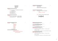
duration and corresponding TV channels. Finally,
meter data measures the viewing behavior of
each one of the viewers, represented by a sequence of
watch/non watch indicators referred to each second of
the day, as illustrated by figure 1. These indicators are
registered independently for each channel.
Figure 1: Representation of a daily viewing pattern for an
individual.
2.2 Requirements
The requirements were gathered through the analysis
of several audience reports, and for on site
day by day usage of the audience analysis program
Telereport[13]. The reports are sufficient broad to embrace
a series of heterogeneous users, ranging from
television to advertising. They cover the most important
aspects of general TV content performance analysis.
However, they do not address the singularities
of advertising spots. The audience analyst are interested,
mainly, to determine the audiences by channel

and/or program, for a set of targets and time periods;
the analysis are never carried through individual
viewers. Viewers are arranged in targets, that closely
relate to socio-demographic information. For example,
a typical target is the AB, consisting of high income
viewers. Time periods range from minute by
minute analysis, to standard audience periods, with 2
or more hours. Periods with more than a day, must
be treated carefully, as the corrective weight change
daily. More details can be found in the work of [3].
2.3 Performance Indicators
Audience analysis define more than a dozen performance
indicators [3]. However, as a regular basis,
audience analysts tend to use only a few. For demonstration
purposes, these paper use only one: TV rating
(rat).
TV rating give us the percentage of the population
that, for a given period, have watched a program/channel.
It tell us the probability of an individual
from the population become a viewer. Let P be
the daily viewers’ panel and W the set of corrective
weights. The rating for a single minute can be calculated
as
|V |
ratminute = ∑
i=0
Vi ∗W(i),V ⊂ P (1)
where V is the subset of individuals that watch television,
on the a specific channel. (1) can be extend to
accommodate a set of minutes M
ratperiod =
∑ ratminute(m)
m∈M
(2)
|M|
However, (2) does not fully address the representativeness
for a target. By definition, most of the performance
indicators relate to a reference value and can
be displayed as percentages. When one say that program
X got a 20% rating, those are the percentage of
the viewers from the panel that share the desire sociodemographic
value, and happened to be watching TV
during the analysis period. Let Tsd be the subset of
the panel that share the desire socio-demographic values
sd. One can determine the sum of the corrective
weigths TW for the target as follows
TW = ∑ W(i) (3)
Tsd∈P
Normalising (2) using (3) give us the representative
value for the desired target
rat = ratperiod
(4)
tw
The rating calculated from (4) is valid measure, not
only for the panel’s viewers, but also for the entire
population of TV viewers.
3 THE MODEL
3.1 Dimensions
From the requirements, each performance indicator is
given context by: (i) Time, detailed to the minute;
(ii) Date, giving access to the daily corrective weight;
(iii) Program, the object of the performance analysis;
and (iv) Socio-demographic information, enabling
target analysis. Date is a regular dimension,
whose characteristics and typical attributes can be observed
in [9] and [6]. Time dimension represents the
daily regularity, but also, typical time periods and a
domain depended referential. The considered periods
are the TV standard 1 : ”02h30-08h00”, ”08h00-
12h00”, ”12h00-14h30”, ”14h30-18h30”, ”18h30-
20h00”, ”20h00-23h00”, ”23h00-24h30”, ”24h30-
26h30”.
Socio-demographic dimension encloses some of
the most used demographic information, such as
Genre, Region, Social Class, Occupation, and Housewife
status. The age information is generally divided
from 5 to 7 intervals. The authors decided
to use the seven interval division: ”[4-14]”,”[15-
24]”, ”[25-34]”, ”[35-44]”, ”[45-54]”, ”[55-64]”,
”>64”. The dimension is populated with all the possible
attribute’s values combination. For the used
data 2 , the value is 6720.
Program dimension encloses all the information
related to a TV show; their name, description, type,
classification and duration. TV shows are classified
with a three level taxonomy, at most. The first level
indicates the topmost classification, e.g. Fiction. Second
level classify the show inside the first level, e.g.
Fiction-Film. Finally, the last level give the maximum
detailed classification for the show, e.g. Fiction-Film-
Comedy. Notice that not all of the shows have a 2nd
or 3rd level of detail. Classification is an enclosed hierarchy
inside the program dimension [9]. However,
it’s not very deep nor its value is unknown; it can be
modelled simply with 3 attributes, one for each level,
with no lack of generality.
With these dimensions, the granularity of the fact
table was fixed at the minute. Note that such a model
doesn’t not addresses the necessities of advertising
spots, which is out of the scope of this work.
3.2 Facts
From a relational point of view, an OLAP cube is the
projection of a relation R, where X1, X2, ..., Xn are
1 For Portuguese TV audience analysis, by the year 2006
2 From 2001

attribute keys and K is the remaining attribute. From
an OLAP point of view, X1, X2, ..., Xn turn to be the
axis of the cube and each value of attribute K is in
the intersection of those axis. We can express K as a
function
K : f (X1,X2,...,Xn) (5)
If one of the axis is omitted from (5), e.g Xn, we
are performing a similar operation as a dimensional
reduction
Knew : f (X1,X2,...,Xn−1) (6)
However, in (5), the result set does not contain
duplicates, because the key set is contained in
the projection result. In (6), to guarantee the
distinction, K needs to be aggregated for each
distinct tuple of the projection set PS set defined as
(x1,x2,x3,...,xn)|xn ∈ dom(Xn). Using the sum as the
aggregation function, the attribute K is summarised as
∑
xn∈dom(Xn)
f (x1,x2,...,xn−1,xn) (7)
The facts in the OLAP Cube does not always directly
point to an a single attribute. Their definition can be
based upon a mathematical operation applied to one
or more data elements. These are generally referred
to as derived data or derived facts [5]. If the operation
defines a ratio3 , the application of (7) results in a nonmeaningful
value, because ratios are non-addictive.
The performance indicators cannot be pre-calculated
and stored directly in the fact table; it must be implemented
as a derived fact.
To be able to properly calculate the performance
indicators for the domain, e.g. rat, a corrective
weight must be used, as can be see in (4). Since
query’s targets are user depended, determined in
runtime by the users’ restrictions over the Sociodemographic
dimension, one can’t pre-determine the
right weight to use. It’s necessary to store all the
possible weights, using (3) to calculate them. For a 4
attribute key cube, we are dealing with a theoretical
value of 15 possible combinations, sum 4 k=1 (4 i
). If one
decided to stored all the possible weights as facts, for
each tuple of the fact table 14 unnecessary values are
stored, as only one is valid for each query. Besides,
the number of possible targets increase this number.
This approach is also not feasible because, for some
indicators, it is necessary to store the weights for
non-viewers, that is, individuals that didn’t watch
television during the analysis period. Fact tables store
only one type of occurrence, in this case, the fact that
some individual watched television; it’s not a good
3 Ratios are not the only type of non-addictive facts.
practice to store the opposite fact too. One must use
a more straightforward approach, using some domain
knowledge.
The data are quota sample-based, which means the
sample was designed to be a representative subset of
the population, regarding some descriptive characteristics.
In this sense, it’s impossible to have an individual
to support simultaneously two or more values for
an attribute. For example, an individual that is present
in the target males with ages ranging from 4 to 14 cannot
be part of other target, females with ages ranging
from 4 to 14.
Property 1. Let Ta be a target with a restriction over
a socio-demographic attribute a,
ta=v1 ∩ta=v2 = /0
If the weights are normalised, which can be done during
the ETL 4 proccess, for any two or more disjoint
subsets, their weights sum up to one.
Property 2. Let Tb be a target with a restriction
over socio-demographic two valued attribute b,
∑ Ta=0∈PW(i) + ∑ Ta=1∈PW(i) = 1 is always true.
Knowing that, it’s possible to create a fact table that
store the weights for all possible targets, including
the non-viewers individuals. That fact table shares
the data and socio-demographic dimensions. Each tuple
in the fact table represent the reference value for
a specific combination of socio-demographic values,
for a given day, applying (3) for each distinct combination.
Figure 2 illustrate the Contact star-schema.
Figure 2: Illustration of the contact starschema model.
The former model provide the weights for all the contacted
individuals, viewers or not, for one day. To calculate
the performance indicators for the domain, e.g.
rating, it’s also necessary to determine the weights of
the viewers. To address this issue, it’s necessary to
create another fact table, that store the viewers’ daily
corrective weight. Since this table is indexed by all
of the dimensions discussed so far, Date, Time, Program
and Socio-Demographic, a tuple represents
4 Extraction Transformation and Loading

a contact of a set of viewers, sharing equal sociodemographic
values, for one minute, a particular program/channel
and a specific day. By observation of
(4), it’s necessary to store the weights and the number
of minutes of the interval. Figure 3 illustrate the
audience star-schema, the main portion of the overall
model.
Figure 3: Illustration of the audience starschema model.
3.3 Optimization of the model
The model is not optimized. The number of theoretical
tuples per day are nearly 9,6 millions (1440 minutes
x 6720 socio-demographic combinations). Even
for the more realistic 1 3 of that value, the table grows
40 million tuples per month. Any optimization of the
model must be thought in terms of gain vs benefit,
as is necessary to create auxiliary aggregate models,
based on requirements.
The first aggregate take advantage of the typical
targets used in TV analysis. Not all of the sociodemographic
combinations are interesting, so, only
8 targets were considered here: Universe, all of the
viewers; Class AB, the most wealthy viewers; 4:14,
young children and teenagers; Housewife, viewers
that are responsible for acquiring essential products
for the house; Adults, viewers above 14 years old;
ABC1 25:34, young active working viewers, from
wealthiest social classes, ranging from 25 to 34 years
old; ABC1 15:34, Young viewers from wealthiest social
classes, ranging from 15 to 34 years old; ABC
25:54, active working viewers, from all social stratus,
except lower classes.
This aggregate represents a 70% reduction of the
tuples needed, compared to the one illustrated on
figure 3. It is necessary to create a new dimension to
accommodate the previous targets. The aggregate’s
model share the Date dimension with the others. The
fact table store the sum of the daily weight for the
target.
Other possible optimization is to aggregate by time
periods. Several reports calculate the indicators for
specific periods, e.g. prime-time. In this model,
the Time dimension is replaced by a new dimension
TimePeriod, a projection of the former, with only the
8 value attribute Period. Consequently, the Program
dimension is incompatible with the new aggregate’s
granularity. From Program, is derived another new
dimension, Channel, with only one attribute, channel.
This represent a reduction of 180% in the first
dimension and 60% in the second. The remaining
dimensions of the main model (figure 3), are compatible.
The fact table store the sum of the daily
weight, for a specific channel, period, date and sociodemographic
combination, and the time interval, in
minutes. Figure 4 illustrates the overall model. The
darker rectangles represent dimensions; the remaining
are the fact tables.
Figure 4: Illustration of the overall model. Bounded tables
are aggregate specific and only exists to increase the models’
performance.
3.4 Evaluation
The evaluation of the model was not based on performance
but on flexibility and simplicity instead. One
of the main goal was to prove the usability of generic
OLAP tools fulfil the needs of the audience analysis
domain, with the same degree of freedom and leading
to the same results. A series of reports were made
using Telereport [13] and the results kept as reference
values. Those reports are expected to be representative
of the daily necessities of an audience analyst.
For lack of space, we do not address the ETL process,
nor it’s evaluation. It suffice to say the OLAP cubes
were created and populated with one year data, using
SQL Server Data Transformations Services [12],
for the ETL, and SQL Server Analysis Services [11]
as a multidimensional engine. For each report, an
MDX query was developed to mimic it, and then executed
against our data. Every execution confirm the
expected reference values, demonstrating that, for the
tested reports, the model is adequate. The benefit of
the aggregates were not tested in performance, but
rather in simplicity. Listing 1 illustrate the necessary

code to implement one of the report. In the particular
case, the query execution display the rating, for the
main targets, by time periods, for one specific channel.
WITH MEMBER Measures . TargetTotal as
’ LookupCube (" ContactTarget ",
"( Measures . weight ,"+ membertostr (
Target . currentmember )+")") ’
MEMBER Measures . rat as
’ Measures . weight / Measures . TargetTotal
/ Measures . num_min ’
, FORMAT_STRING =’ Percent ’
SELECT { Target . currentmember } ON COLUMNS ,
time . Period . Members ON ROWS
FROM AudienceTarget
WHERE ( Measures .rat , Program . Canal .[2])
Listing 1: The rating for the main targets by time periods
for channel 2 using the target aggregate
The code is rather simple because each target
weight is pre-calculated in the ContactTarget aggregate.
The LookupCube function lookup the value for
each target querying it. With the absence of this cube,
each target weight is calculate in runtime, looking up
each socio-demographic variable that made up the target.
Not only the execution times rise up, but also the
query’ code.
4 Conclusion
This work presents a dimensional model capable
to address the specificities of quota sample based data.
The goal was twofold; first, to demonstrate that is
possible to address audience analysis requirements,
using non-proprietary repositories and technologies;
second, to present a possible solution to other domains
where data is also quota sample based. In the
audience domain, the data tendencies are corrected by
a daily individual weight, that must be taken into account
if the indicators are meant to be representative
to the entire population, not just the panel’s individuals.
To deal with the audience performance indicators,
mostly non-addictive and quota depended, is necessary
to normalise each one with a reference value, calculated
from the corrective daily weights. The present
solution lay on the creation of an auxiliary contact table
to store daily weights for each possible combination
of socio-demographis values. The authors transform
this way the non-addictive facts into addictive
ones, sacrificing the capability of pre-calculated their
values and store them into a fact table directly. All of
the calculus must be done in runtime. To ensure an
efficient solution, is necessary to create a series of domain
dependant aggregates, with specific dimension
models. The performance indicators test results, using
both proprietary program and generic OLAP tools
with the discussed model, have matched.
Authors think the same methodology is appropriate
to other domains if the data is quota sample based
and the performance indicators values are always relative
to the subset of the sample used in their calculus.
REFERENCES
[1] Yvonne M. M. Bishop, E. F. Fienberg, and P. W. Holland.
Discrete multivariate analysis : theory and practice.
The MIT Press, 1975.
[2] EF Codd, SB Codd, and CT Sally. Providing
OLAP to user-analysis. Technical report,
http://www.arborsoft.com/essbase/wht ppr/coddps.
zip, 1993.
[3] Nuno Datia. Aplicação de técnicas de apoio à decisão
a dados de audimetria. Master’s thesis, Faculdade de
Ciências e Tecnologia - Universidade Nova de Lisboa,
2006.
[4] W. Edwards Deming and Frederick F. Stephan. On a
least squares adjustment of a sampled frequency table
when the expected marginal totals are known. Annals
of Mathematical Statistics, 11(4):427–444, 1940.
[5] C. Imhoff, N. Galemmo, and J.G. Geiger. Mastering
Data Warehouse Design: Relational and Dimensional
Techniques. Wiley, 2003.
[6] WH Inmon. Building the data warehouse. John Wiley
& Sons, Inc. New York, NY, USA, 2005.
[7] N. Jukic, B. Jukic, and M. Malliaris. Online Analytical
Processing (OLAP) for Decision Support. In
Handbook on Decision Support Systems. Springer,
2008.
[8] R. Kimball, L. Reeves, M. Ross, and W. Thornthwaite.
The Data Warehouse Lifecycle Toolkit. Wiley, 1998.
[9] R. Kimball and M. Ross. The Data Warehouse Toolkit:
The Complete Guide to Dimensional Modeling. Wiley,
2002.
[10] MediaSoft Kimono. http:// www. kubik. it/
kimono_ en. html , last acessed on May 2008.
[11] Sql Server Analysis Services. http://
technet. microsoft. com/ pt-br/ sqlserver/
bb671220(en-us). aspx , last acessed on May 2008.
[12] Sql Server Data TRansformations Services. http://
www. microsoft. com/ technet/ prodtechnol/ sql/
2000/ deploy/ dtssql2k. mspx , last acessed on May
2008.
[13] Markdata Telereport. http:// www. markdata. net/
v2/ , last acessed on May 2008.
[14] Rene Weber. Methods to Forecast Television Viewing
Patterns for Target Audiences. In Communication Research
in Europe and Abroad –Challenges of the First
Decade, 2003.