A OPEN PIT MINING AÇIK OCAK MADENCİLİĞİ
A OPEN PIT MINING AÇIK OCAK MADENCİLİĞİ
A OPEN PIT MINING AÇIK OCAK MADENCİLİĞİ

Create successful ePaper yourself
Turn your PDF publications into a flip-book with our unique Google optimized e-Paper software.
Chapter - A<br />
<strong>OPEN</strong> <strong>PIT</strong> <strong>MINING</strong>
2<br />
23 rd
23 rd <br />
Electric Drive Mining Class Wheel Loaders as Primary<br />
Production Tools<br />
A. Wood<br />
Institution of Engineering and Technology, UK<br />
ABSTRACT Mechanical wheel loaders are traditionally considered as support equipment,<br />
back up to excavators and utilized as “clean up” equipment. This paper discusses the benefits<br />
of employing large Electric Drive, Mining Class, Wheel Loaders as opposed to hydraulic<br />
excavators in high production low cost mining operations, and the differentiation between<br />
Electric Drive Wheel Loaders and Mechanical Drive Wheel Loaders. Large Electric Drive<br />
Wheel Loaders, with bucket capacities up to 56m³ and payloads of 72 Tonnes, combined with<br />
fuel saving Electric Power Regeneration technology, demonstrate competitive advantages<br />
against hydraulic excavators in availability, production and more importantly Total Cost of<br />
Ownership (TCO). Electric Drive Wheel Loaders have been available for over forty years, and<br />
the fuel saving technology developed for this class of wheel loader is now utilized in other<br />
mine site vehicles such as haul trucks. This paper compares design features, productivity,<br />
operational costs, maintenance issues and applications.<br />
1 WHEEL LOADER DESIGN<br />
1.1 Mechanical Drive Wheel Loaders<br />
Mechanical drive wheel loaders are found in<br />
many applications and sizes up to the<br />
CAT994, (35 Tonne Payload), and Komatsu<br />
WA1200 (38 Tonne Payload). (Anon 2012)<br />
These larger classes of wheel loaders are a<br />
familiar and much used support equipment<br />
for mine sites, assisting in everything from<br />
infrastructure development to back up<br />
production.<br />
Figure 1. CAT994 35 Tonne Mechanical<br />
Drive Wheel Loader.<br />
Figure 2. Komatsu WA1200 36 Tonne<br />
Mechanical drive Wheel Loader<br />
All main functions of propel, steering and<br />
load/unload cycles are powered directly from<br />
3
A. Wood<br />
hydraulics, couplings and gear units to the<br />
diesel engine.<br />
1.2 Electric Drive Wheel Loaders<br />
Electric Drive Wheel loaders are found in<br />
high production mining applications, mainly<br />
as primary loading tools. The size and class<br />
of this type of wheel loader starts at Joy<br />
Global LeTourneau L-950, (25 Tonne<br />
payload), and ranges up to the L-2350 (72<br />
Tonne payload), which is twice the capacity<br />
of the largest mechanical wheel loader, and<br />
has comparative payload to 40m³ hydraulic<br />
shovels, (PC8000, EX8000 class). (Fleet,<br />
2012)<br />
Figure 3. LeTourneau L-2350 Electric Drive<br />
72 Tonne Wheel Loader.<br />
1.2.1 Design Features<br />
The most significant design feature of<br />
electric drive wheel loaders is electric power<br />
regeneration, which is captured and fully<br />
reutilized. (Fleet, 2012)<br />
The main drive diesel engine is coupled<br />
directly to a generator, which provides the<br />
electric power to operate the loader.<br />
Each wheel is mounted on an individual<br />
wheel driver assembly, consisting of a<br />
planetary transmission and electric motor.<br />
The loading cycle consists of propel to<br />
bank, dig, reverse propel, propel to truck or<br />
hopper, dump, and propel back to start of<br />
cycle. At each point in propel, the loader<br />
consumes fuel on acceleration, and at steady<br />
state. However, on deceleration, which is<br />
done through electromagnetic braking, the<br />
wheel motors are used as generators, which<br />
feed power back to the power control system.<br />
Figure 4. Electric Drive Wheel Loader<br />
Layout.<br />
This regenerated power is used to drive<br />
the generator, which is directly coupled to<br />
both the diesel engine and the main hydraulic<br />
system. As the regenerated power drives the<br />
generator, there is no load on the diesel<br />
engine, and fuel supply is cut off. This is the<br />
basic design feature which significantly<br />
reduces fuel consumption of this type of<br />
loading tool.<br />
Electromagnetic primary braking reduces<br />
maintenance time and replacement costs<br />
associated with mechanical disc brakes.<br />
As the wheel loader has independent four<br />
wheel drive, power and speed are controlled<br />
to each wheel, which allows power to be<br />
reduced to any individual wheel which starts<br />
to slip, regaining traction. This prolongs tire<br />
life through reduced wheel spin, and through<br />
correct individual wheel speed when turning.<br />
(Fleet, 2012)<br />
An electric drive wheel loader can<br />
continue to perform its function if one of the<br />
wheel motors fails, allowing for reduced, but<br />
continued production, and the ability to<br />
propel back to the maintenance location,<br />
under its own power, when replacement is<br />
ready.<br />
This system has stepless forward and<br />
reverse propel, negating any need for<br />
standard mechanical drive train. Fewer<br />
mechanical parts allows for less maintenance<br />
and higher availability than mechanical<br />
based systems. This also allows for<br />
significantly less consumption of lubrication<br />
fluids, making it an altogether more<br />
environmentally friendly tool.<br />
Electric motors are brushless DC,<br />
requiring no maintenance, other than bearing<br />
4
23 rd <br />
change out at defined intervals, and operate<br />
on the switched reluctance principle.<br />
Wheel loaders do not require ancillary<br />
floor clean up equipment, as they can<br />
perform this exercise themselves. (Ozdogan,<br />
2012)<br />
2 PRODUCTIVITY<br />
Wheel loaders are highly flexible tools,<br />
allowing for the quickest relocation. They<br />
can be the first loading tool to the digging<br />
face after a blast, ensuring quickest restart of<br />
production, and can be quickly deployed to<br />
alternate selective and material blending<br />
requirement locations.<br />
Standard track mounted production tools<br />
such as Rope Shovels and Hydraulic<br />
excavators, have a revolving upper structure,<br />
and only require relocation when the material<br />
to be excavated is out of reach. This typically<br />
leads to sub thirty second load cycles for<br />
smaller class equipment and sub thirty five<br />
second cycles for larger equipment.<br />
Wheel loader performance relies more on<br />
operators to minimize travel distances.<br />
(Fleet, 2012). Well trained operators can<br />
achieve thirty second load cycles on wheel<br />
loaders, with a more typical figure for<br />
electric drive wheel loaders of thirty five to<br />
forty seconds, and a few seconds longer for<br />
mechanical drive wheel loaders in the same<br />
application, due to mechanical performance.<br />
(Klink 2012)<br />
Rope Shovels and Hydraulic excavators<br />
have more digging power than wheel loaders<br />
due to their weight and design. Each<br />
equipment type has its suitable application.<br />
In adequately blasted, or free digging<br />
applications, electric drive wheel loaders can<br />
offer competing productivity, at lower total<br />
cost than diesel powered hydraulic<br />
excavators, by using a larger capacity wheel<br />
loader to make up the productivity gains lost<br />
by cycle time. (Anon, 2011)<br />
Example 1. Productivity<br />
15m³ Hydraulic excavator – 27 Tonne<br />
91 Tonne payload truck<br />
3600 Seconds in one hour<br />
90% Operator Efficiency<br />
Equation 1. Loading cycles<br />
<br />
<br />
N = Number of Loading Cycles<br />
P t = Truck payload (Tonne)<br />
P = Wheel Loader payload (Tonne)<br />
<br />
<br />
Equation 2. Time to load truck<br />
<br />
T = Time to load truck (Sec)<br />
T c = Time for individual load cycle (Sec)<br />
T s = Time for truck spotting (Sec)<br />
<br />
Equation 3. Trucks Loaded Per Hour<br />
<br />
<br />
N h = Number of trucks loaded in one hour<br />
S h = Seconds in one hour<br />
O e = operator Efficiency<br />
<br />
<br />
Equation 4. Hourly Production<br />
P hr<br />
<br />
= Hourly productivity (Tonne)<br />
<br />
<br />
Example 2 Productivity<br />
19m³ Electric drive wheel loader<br />
34.5 Tonne wheel loader payload<br />
5
A. Wood<br />
91 Tonne payload truck<br />
3600 Seconds in one hour<br />
90% Operator Efficiency<br />
Loading cycles<br />
Use equation 1.<br />
<br />
<br />
Time to load truck<br />
Use equation 2.<br />
<br />
Trucks Loaded Per Hour<br />
Use equation 3.<br />
<br />
<br />
Hourly Production<br />
Use equation 4.<br />
<br />
<br />
<br />
Productivity Example 3<br />
21m³ Hydraulic Excavator<br />
38 Tonne wheel loader payload<br />
91 Tonne payload truck<br />
3600 Seconds in one hour<br />
90% Operator Efficiency<br />
Loading cycles<br />
Use equation 1.<br />
<br />
<br />
Time to load truck<br />
Use equation 2<br />
<br />
Trucks Loaded Per Hour<br />
Use equation 3.<br />
<br />
<br />
<br />
Hourly<br />
Production<br />
Use equation 4.<br />
<br />
<br />
In this illustration, a 19m³ payload,<br />
electric drive wheel loader, is equally as<br />
productive as a 15m³ hydraulic excavator<br />
with similar production availability. (Binns,<br />
2012)<br />
The capital purchase costs and life<br />
expectancy are similar. The advantage of<br />
electric drive wheel loaders is seen in the<br />
operational costs, which are presented in the<br />
next section. (Binns, 2012)<br />
A 21m³ hydraulic shovel compared to the<br />
19m³ electric drive wheel loader will be<br />
more productive if matched for three pass<br />
loading, but will have a higher capital cost<br />
and higher operational cost per tonne loaded.<br />
3 OPERATIONAL COSTS<br />
Fuel consumption is a major cost for all<br />
diesel powered loading tools, compared to<br />
electric powered equipment such as rope<br />
shovels, and to a lesser extent electric<br />
powered hydraulic shovels.<br />
Fuel consumption is minimized on electric<br />
drive wheel loaders through efficient use of<br />
regenerated energy. Mechanical systems<br />
waste this potential energy saving through<br />
heat in friction disks for braking.<br />
Brake Specific Fuel Consumption (BSFC)<br />
is a measure of fuel efficiency within a shaft<br />
reciprocating engine. It is the rate of fuel<br />
consumption divided by the power produced.<br />
It may also be thought of as power-specific<br />
fuel consumption, for this reason. BSFC<br />
allows the fuel efficiency of different<br />
reciprocating engines to be directly<br />
compared.<br />
Equation 5 Brake Specific Fuel Consumption<br />
<br />
<br />
P = Power produced in kW<br />
C f = Fuel Consumption<br />
(L/hour @ RPM for stated power)<br />
6
23 rd <br />
D f = Fuel Density<br />
A typical value of fuel density is<br />
854g/liter. (Range 849-960g/l)<br />
A typical BSFC value for mining duty<br />
diesel engines in loaders, excavators and<br />
trucks is 200g/kW.hr. (Range 180g/kW.hr<br />
for highly efficient engines to 250g/kW.hr<br />
for less efficient engines)<br />
Transposing the formula to give max fuel<br />
burn at 100% engine load, on typical BSFC.<br />
<br />
<br />
Example 4. Fuel consumption at 100%<br />
Engine Load<br />
Engine Power = 940kW @ 1800RPM<br />
BSFC = 200g/kW.hr<br />
Df = 854g/L<br />
<br />
<br />
<br />
<br />
A typical electric drive wheel loader has<br />
an average engine load factor of 39%(Fleet<br />
2012), compared to 60%+ for mechanical<br />
systems. This is due to regenerated power<br />
being fed back on electric drive wheel<br />
loaders, and used to power the units<br />
hydraulic systems. On power regeneration,<br />
fuel to the engine is cut off, resulting in the<br />
significantly lower average engine load<br />
factor.<br />
Fuel cost comparison of a typical 15m³<br />
Hydraulic shovel versus 19m³ electric wheel<br />
loader, as described in the productivity<br />
details on previous page.<br />
Hydraulic shovel 15m³<br />
Engine Power 940kW@1800 RPM<br />
Fuel Consumption:-<br />
at 100% Engine Load = 220 lph<br />
at 65% Average Cycle Load = 143 lph<br />
Over 5000 hours = 715,000 litres<br />
Fuel Consumption<br />
19m³ Electric Drive Wheel Loader<br />
Engine Power 899kW @ 1800RPM<br />
Fuel Consumption<br />
at 100% Engine Load = 208 lph<br />
at 39% Average Cycle Load = 81 lph<br />
Over 5000 hours = 405,000 litres<br />
Fuel Consumption<br />
Showing a 310,000L fuel saving for the<br />
same production, over a 5000 hour / one year<br />
period.<br />
Major engine overhauls are typically<br />
based on fuel consumed.<br />
While life-to-overhaul can be expressed in<br />
hours, some diesel engine manufacturers<br />
prefer to focus on average design life-tooverhaul<br />
in terms of liters of fuel consumed<br />
as a more accurate measure which better<br />
reflects high engine load operating factors.<br />
Depending upon duty cycle, the average<br />
design life-to-overhaul for a 2MW mining<br />
duty engine exceeds 3,785,000 liters of fuel<br />
consumed and for 1.5MW this is 3,312,000<br />
liters. (Cummins, 2008)<br />
Electric drive wheel loaders having fuel<br />
saving technology, provide major engine<br />
overhaul at over 20,000 operational hours.<br />
Fewer mechanical parts on an electric<br />
drive wheel loader, result in reduced parts<br />
and lubrication usage and reduced<br />
maintenance costs.<br />
4 MAINTENANCE<br />
Critical components to maintain on an<br />
electric drive wheel loader are the engine,<br />
tires and hydraulic systems. (Fleet, 2012)<br />
Tire life can be extended with use of tire<br />
chains. (Ozdogan, 2012)<br />
Engine, hydraulic and welding<br />
maintenance requirements are similar to any<br />
other hydraulic excavator or mechanical<br />
wheel loader<br />
Switched Reluctance wheel motors only<br />
require new bearings on high hour overhauls.<br />
(Fleet, 2012)<br />
Modern electronic control systems on<br />
electric drive wheel loaders provide a stable<br />
electrical maintenance platform.<br />
As primary loading tools, electric drive<br />
wheel loaders are equipped with full service<br />
operational and maintenance trouble<br />
shooting controls systems, to assist with<br />
productivity and maintenance management.<br />
7
A. Wood<br />
5 APPLICATIONS<br />
Electric drive wheel loaders have slightly<br />
lower breakout forces than hydraulic<br />
excavators, and they do not have an option to<br />
act as a back hoe.<br />
Electric drive wheel loaders are used<br />
around the world as primary loading tools in<br />
high production mines, covering iron, copper<br />
and gold ore, as well as in hard overburden<br />
and coal removal applications.<br />
The flexibility that a wheel loader offers,<br />
makes them ideal for selective mining and<br />
blending operations.<br />
6 CONCLUSIONS<br />
Electric drive wheel loaders make use of<br />
technology to provide more economic and<br />
reliable production. Capital costs should be<br />
considered against the operational costs,<br />
specifically fuel consumption, and the<br />
productivity potentials for the equipment. An<br />
electric drive wheel loader, 5m³ larger than a<br />
hydraulic excavator can provide the same<br />
production as that hydraulic excavator, at a<br />
lower cost, and provide a fully flexible<br />
primary loading tool.<br />
REFERENCES<br />
Anon. 2011, personal communication, LeTourneau<br />
Wheel Loader Operator Trainer.<br />
Anon. 2012, Website Reference Machine Data<br />
sheets, mining.cat.com, www.komatsu.com.<br />
Binns, D, personal communication, Regional<br />
Director, Joy Global<br />
Cummins, 2008, Media release, Cummins Fuel-<br />
Efficient QSK Engines Optimized,<br />
www.cummins.com<br />
Fleet, M, 2012, personal communication,<br />
LeTourneau Regional Manager.<br />
Klink, D, 2012, personal communication, Joy Global<br />
Regional Service Manager.<br />
Ozdogan, M, 2012 personal communication, Ideal<br />
Machinery and Consultancy Ltd, Ankara, Turkey<br />
8
23 rd <br />
Gold-Mining and Ornamental Stones Quarrying in The Wadi<br />
Hammamat, Ancient Egypt: Geological Framework and<br />
Techniques<br />
M. Coli & M. Baldi<br />
Dip. Scienze della Terra, UNIFI - Italy<br />
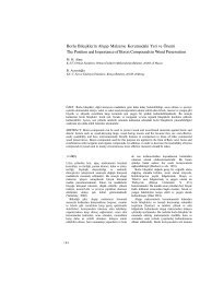
ABSTRACT In this paper we outline the cultural and technical context and the geological<br />
framework of the outstanding gold mining and prized ornamental stone quarrying activities<br />
which were carried out in the Wadi Hammamat (‘Valley of the Baths’) in Ancient Egypt.<br />
Quarrying and mining remains preserve traces of man’s activity and of technical skill,<br />
therefore they represent “landscape archives” and valuable cultural heritage sites where the<br />
traces of work, technology, organization and social life can be studied in order to hand them<br />
down to posterity and open a window on an ancient world, almost unknown to most. The<br />
results of our survey confirm the correctness of ancient geological knowledge as shown in the<br />
famous Turin Mine Papyrus, and in general highlight a good knowledge of the territory, such<br />
as the role played by the geological setting in providing materials and driving the extraction<br />
techniques, both in the Pharaonic and Roman periods.<br />
1 INTRODUCTION<br />
From ancient times until today the use of<br />
natural stone and mine resources has been a<br />
main element for human activity. Historical<br />
extraction sites have been lately described as<br />
“landscape archives”: sites or areas where<br />
the traces of work, technology, organization<br />
and social life are preserved and where they<br />
can be studied in order to hand them down to<br />
posterity and open a window on an ancient<br />
world, almost unknown to most.<br />
In the last decades there was a renewed<br />
interest for ancient quarry and mine<br />
exploitation in the scientific community,<br />
public administrations and in the area of the<br />
cultural tourism. Several cultural activities<br />
have grown based on a rediscovery and<br />
reappraisal of ancient quarries and mines,<br />
such as the creation of eco-museums and<br />
other didactic activities at various levels.<br />
The study of the historical quarrying and<br />
mining sites highlights the diffusion of a<br />
shared basic knowledge among ancient<br />
civilizations and the fact that technologies<br />
were strictly linked to the social and cultural<br />
aspects of each population.<br />
At the same time these recent studies<br />
outline both a good knowledge of the<br />
territory and of its geological setting which<br />
was used at the best in developing the right<br />
exploitation techniques. That was<br />
particularly true in Ancient Egypt (Arnold,<br />
1991; Aufrère, 1991).<br />
The Wadi Hammamat represents a<br />
“landscape archive” where it is possible to<br />
study the ancient quarrying and mining<br />
processes and the social and geological<br />
knowledge context in which these processes<br />
where developed.<br />
Previous studies (Ortolani, 1989; Arnold,<br />
1991; Klemm & Klemm, 1993/2008; Meyer,<br />
9
M. Coli, M. Baldi<br />
1997; Aston et al., 2000; Klemm et al., 2001;<br />
Sidebotham et al., 2008; Harrell & Storemyr,<br />
2009; Bloxam, 2010), and common<br />
knowledge, were taken into account in order<br />
to create a general historical, social and<br />
economic framework for our research, and<br />
also to date quarries and mines and stone<br />
working technologies (Bessac, 1986; Herz &<br />
Waelkens, 1988; Rockwell, 1990; Waelkens<br />
et al., 1992; Bessac, 1993, 1998; Bessac et<br />
al., 1999; Matthias, 2002; Giampaolo et al.,<br />
2008).<br />
We focussed our research on the<br />
relationships between geology, quarrying<br />
and mining activities with the aim of<br />
recovering ancient excavation techniques.<br />
In our fieldwork, we performed a field<br />
survey of the whole area, all the data<br />
referring to quarrying and mining activity<br />
were implemented, by means of a Palm-PC,<br />
in a GIS, based on Google Earth® images,<br />
with the GPS position in WGS84 coordinate<br />
system.<br />
2 GEOLOGICAL CONTEXT<br />
In the surveyed area (Fig.1), the Precambrian<br />
basement, igneous and metamorphic rocks of<br />
the Neoproterozoic (1,000-542Ma) Arabian-<br />
Nubian Shield, outcrops all along the Middle<br />
Eastern Desert Ridge, below the Meso-<br />
Cainozoic sedimentary cover.<br />
Figure 1. Geological sketch map of the area<br />
surrounding the Wadi Hammamat<br />
(highlighted) in the Eastern Desert Ridge<br />
(modified from Fowler & Osman 2001).<br />
The Precambrian outcrops in a broad<br />
structural high which is bounded by<br />
Cretaceous to Miocene continental to<br />
shallow-water formations on both the east<br />
and west sides, Holocene continental<br />
deposits are present in the Nile Valley and<br />
on the Red Sea coastal plane (Said, 1962;<br />
Said Ed., 1990; Tawadros, 2001; Sampsell,<br />
2003). In the core of the ridge, south of the<br />
Wadi Hammamat there is the Sibai Dome,<br />
while the Meatiq Dome lies at its north<br />
(Eliwa et al., 2006).<br />
In the Wadi Hammamat area, where there<br />
are with the most important historically<br />
exploited natural resources, there are<br />
outcrops of the clastic deposits of the<br />
Hammamat Group, of metabasites of the<br />
Ophiolitic Melange and of granitic bodies.<br />
The Hammamat Group is intruded, and<br />
locally contact metamorphosed, by the<br />
younger granite bodies, as the Um Ba’anib<br />
and the Atallah felsic plutonic complexes,<br />
intruded until about 550Ma (Akaad &<br />
Noweir, 1969; Essawy & Abu Zeid, 1972;<br />
Unzog & Kurz, 2000; Eliwa et al., 2006) and<br />
the Um Had granitic pluton (Akaad &<br />
Noweir, 1980). Faults and dikes, related to<br />
the late granitic intrusion, cross-cut the older<br />
metabasites and granites.<br />
The Hammamat Group was deposited in a<br />
major fluvial system of continental<br />
proportions (Wilde & Youssef, 2002)<br />
developed in fault-bounded basins formed<br />
due to N-S to NW-SE directed extension<br />
(Abdeen & Greiling, 2005).<br />
The Hammamat Group is subdivided into<br />
two formations: the upper Shihimiya Fmt.<br />
and the lower Igla Fmt.. The Shihimiya Fmt.<br />
comprises, from top to bottom, the following<br />
members: Um Hassa Greywacke, Um Had<br />
Conglomerate, Rasafa Silstone. The Igla<br />
Fmt. is composed by arenites,<br />
conglomerates, wakes and red-purple to<br />
brick-red haematitic siltstones.<br />
The Hammamat Group (Akaad & Noweir,<br />
1969) consisted, originally, of immature to<br />
sub-mature interbedded sequences of<br />
mudstones, siltstones, quartz arenites,<br />
10
23 rd <br />
greywackes and conglomerates that belong<br />
to the molasse facies; the sedimentary<br />
succession is up to 4,000m in thickness and<br />
aged to 616-590Ma.<br />
The geological texture of the Hammamat<br />
Group characterizes and gives prizes to the<br />
ornamental stone here quarried.<br />
Lamination and bedding structures are<br />
well-developed in the metasiltstones and<br />
metagreywackes, they resemble alternating<br />
parallel laminae and thin beds (up to 10cm<br />
thick) of darker and lighter material of<br />
different grain size in matrix or not.<br />
Metasiltstones and metagreywackes are<br />
much more abundant than<br />
metaconglomerates, these last are fine<br />
grained and exhibit a variety of colors:<br />
greenish-grey, dark-grey, brown, and brickred,<br />
cross-bedded layers of metagreywacke<br />
can reach up to 40m in thickness. The<br />
metaconglomerates are massive and poorly<br />
sorted, and composed of oval, rounded and<br />
sub angular rock fragments from a few to<br />
15cm in diameter, cemented by a finer<br />
greenish-grey to brownish matrix. The<br />
pebbles are of various rock types, including<br />
volcanic rocks, granitoids, and reworked<br />
fine-grained sedimentary rocks. In the Wadi<br />
Hammamat area clasts were derived from<br />
30% mafic rocks, 25% granodiorite, 25%<br />
intermediate volcanics and 20% felsic<br />
volcanics (Holail & Moghazi, 1998).<br />
The first modern geological map of the<br />
Wadi Hammamat area, surveyed at the scale<br />
1:40,000, was done by El-Ramly & Akaad<br />
(1960), the area was then mapped by Akaad<br />
& Noweir (1978) at the scale 1:50,000 and<br />
with a much more geostructural detail by<br />
Fowler & Osman (2001). However, before<br />
all these studies, the “geology” of the Wadi<br />
Hammamat area was also reported in a<br />
papyrus scroll, now displayed in the<br />
Egyptian Museum in Turin (Italy) and<br />
known as the “Turin Mine Papyrus”. The<br />
Papyrus dates back to the reign of Ramesses<br />
IV (20 th Dynasty, New Kingdom) and<br />
probably was drawn by the scribe<br />
Amennakht during one of the quarrying<br />
expeditions to the Wadi Hammamat ordered<br />
by the Pharaoh (1,153-1,147 B.C.).<br />
According with the reconstruction by<br />
Harrell & Brown (1992), we georeferenced<br />
the Papyrus map on Google-Earth® images<br />
(Fig.2).<br />
Figure 2. Harrell & Brown 1992<br />
interpretation of the Turin Mine Papyrus<br />
georeferenced on Google Earth® image, the<br />
colours correspond as reported in the<br />
Papyrus and result consistent with the main<br />
geological units.<br />
That resulted very fruitful for a fieldwork<br />
based on WGS84 GPS data. The Papyrus<br />
shows some coloured areas, which,<br />
according to the reconstruction by Harrell &<br />
Brown (1992), well fit with the main<br />
geological units, and for this reason the<br />
Papyrus can be considered to be the oldest<br />
geological map in the world.<br />
3 GOLD-ORES AND MINE<br />
EXPLOITATION TECHNIQUES<br />
Gold in Egypt occurs both in alluvial placers<br />
and in primary ore bodies in quartz veins<br />
(Klemm et al., 2001), like in the Wadi<br />
Hammamat area. Quartz veins intruded into<br />
the surrounding rocks during the latest<br />
plutonic activity of the Um Ba’anib and<br />
Atallah plutons.<br />
Early techniques consisted in making a<br />
fire against the rock outcrop in order to heat<br />
it up, and then douse it by cold water<br />
(Ogden, 2000; Klemm et al., 2001). The<br />
sudden change in temperature crumbled the<br />
rock revealing the presence of gold; this<br />
technique was used in open-cast trenches<br />
following the quartz veins along the surface.<br />
The rock was then powdered and ‘washed’,<br />
11
M. Coli, M. Baldi<br />
exactly as it was done with alluvial gold.<br />
(Vercoutter, 1959; Ogden, 2000; Sidebotham<br />
et al., 2008). Thanks to newer excavation<br />
techniques, which were performed using<br />
copper, bronze and later iron tools,<br />
Egyptians were able, from the Late New<br />
Kingdom (Ogden, 2000; Klemm et al., 2001;<br />
Sidebotham et al., 2008), to re-open the<br />
previous abandoned mines digging shafts<br />
horizontally or diagonally into the sides of<br />
mountains following the quartz veins<br />
(Fig.3).<br />
Figure 3. Main shaft of a gold mine<br />
following a mineralized quartz vein.<br />
In order to maintain stability, the shafts<br />
had the entrances reinforced by dry-stone<br />
walls and platforms at various levels to help<br />
in raising and lowering workers, baskets,<br />
tools, and ore.<br />
The organization of mining operations<br />
during the Ptolemaic period, II Century B.C.,<br />
was described with full particulars by a<br />
Greek author, Agatharchides of Cnidus, as<br />
recorded one century later by the historian<br />
Diodorus Siculus (Bibliotheca Historica, III,<br />
12-14; for the text see point 12, 13, 14 at:<br />
http://penelope.uchicago.edu/Thayer/E/Rom<br />
an/Texts/Diodorus_Siculus/3A*.html).<br />
The evidence in the mines and settlement<br />
sites fit perfectly with his description of that<br />
hard and crude job.<br />
That general organization of the mining<br />
work implies a whole chain of organized<br />
staff: many slaves who were either prisoners<br />
of war or convicts (“damnata ad metalla”),<br />
but also paupers, often with their entire<br />
families - for the rough excavation and<br />
transport work and for milling and washing<br />
the ore, guardians, a few skilled free workers<br />
to maintain control, choose the rock and melt<br />
the gold, officials, and at least a probator<br />
(geologist) for managing the mines and the<br />
gold transport.<br />
4 ORNAMENTAL STONES AND<br />
EXPLOITATION TECHNIQUES<br />
In the Wadi Hammamat area there were<br />
located the quarries of four prized<br />
ornamental stones:<br />
1 - Bekhen-stone<br />
2 - “Breccia Verde Antica”<br />
3 - Wadi Umm Fawakhir granite<br />
4 - “Serpentina Moschinata”.<br />
All these stones were prized ornamental<br />
stones that impressed anyone with wealth<br />
and power (Coli & Marino, 2008), too<br />
valuable for common use, and therefore<br />
reserved for public and propaganda<br />
purposes.<br />
4.1 Bekhen-stone<br />
The bekhen-stone (as it was called in ancient<br />
Egypt) is the famous dark grey/green<br />
ornamental stone formerly called Basanites,<br />
(Lapis Basanites - probably from the same<br />
ancient Egyptian : Harrell 1995)<br />
(http://www.museo.isprambiente.it/schedeM<br />
appa.page?docId=707).<br />
The analysts of the XIX century could<br />
only analyze very small samples from<br />
artifacts of which they did not know the<br />
provenance, and because of the mineropetrographic<br />
composition of the stone<br />
samples, they classified them as a special<br />
“type of basalt”. Subsequently, when a<br />
similar type of basalt (typical from hot-spot<br />
source) was found, it was called Basanite.<br />
But Basanites bekhen-stone is a<br />
continental clastic sedimentary rock, only<br />
locally metamorphosed by contact<br />
metamorphism due to plutonic intrusions,<br />
which was derived from the dismantling of<br />
mainly basic rocks, and also old granite and<br />
carbonate ones, so that the minero-<br />
12
23 rd <br />
petrographic assemblages are the same,<br />
though the geological origin is totally<br />
different.<br />
Therefore for this ornamental stone the<br />
name Basanite has been dismissed and now<br />
the original name is used, bekhen-stone.<br />
During our field work we surveyed several<br />
quarries that exploited the bekhen-stone.<br />
4.1.1 Geology<br />
In the Wadi Hammamat, the bekhen-stone<br />
outcrops for about 2km, corresponding to the<br />
Um Hassa Greywacke Member of the<br />
Hammamat Group and consisting of (Aston<br />
et al. 2000) dark greenish-grey to mainly<br />
greyish-green, medium- to very finegrained,<br />
occasionally pebbly, chloritic<br />
greywacke, mainly composed of fine to very<br />
fine sand grains (0.06-0.2mm) and darkgrey-green,<br />
basalt-looking, siltstone. This<br />
last lithofacies outcrops mainly in the<br />
eastern side of the quarry area.<br />
The grains are mostly quartz, with minor<br />
oligoclase-andesine plagioclase and felsic to<br />
intermediate volcanic rock fragments plus<br />
rare muscovite. The matrix is composed by<br />
chlorite and sericite plus minor amounts of<br />
epidote and calcite. The layering dips 45°<br />
towards the east.<br />
The bekhen-stone rock-mass presents<br />
three joint sets: two vertical, at about 90°<br />
and trending around E-W and N-S<br />
respectively, and one sub-horizontal; the<br />
joints are up to a few meters spaced so they<br />
delimit natural blocks up to a few cubic<br />
meters in volume.<br />
4.1.2 - Quarrying<br />
The slopes of the wadi are generally covered<br />
by debris, therefore we can suppose,<br />
according to the general geomining<br />
concepts, that the first quarries were opened<br />
in the lower outcrops at the base of the<br />
slopes. When the highness of the quarry face<br />
made further exploitation of the quarry<br />
difficult, in combination with the difficulty<br />
posed by overhanging debris, quarriers<br />
moved the quarrying activity to an upper<br />
outcrop, creating access with tracks and<br />
ramps and sledge-ways for handling blocks<br />
and setting up new logistics.<br />
Most recently Spencer (2011) reports the<br />
finding of “four hitherto unknown Early<br />
Dynastic quarries located at high elevations<br />
on the Bekhen Mountain”.<br />
Quarries were opened in the main natural<br />
outcrops, on the cliffs bounding the wadi.<br />
Quarriers used the three sets of joints (Fig.4)<br />
as preferential surfaces to dismantle the<br />
rock-mass into blocks and then let them fall<br />
down the slope to the wadi floor.<br />
Figure 4. The main outcrop of the bekhenstone:<br />
the three almost orthogonal joint sets<br />
which were used in order to dismantle the<br />
rock and collect cut blocks down-slope.<br />
One of the main problems was to<br />
dismantle, but keep intact while being<br />
transported down-slope, a block of stone the<br />
right size for the ordered statue or<br />
sarcophagus. According to an inscription,<br />
Meri, the leader of a quarrying expedition in<br />
the reign of Amenemhet III (ca.1,810 B.C.),<br />
in order to keep the stone blocks intact<br />
down-slope, built the first inclined plane<br />
(sledge-way) to slide the blocks down<br />
(Montet, 1959). The Romans built a very<br />
long sledge-way in order to bring down<br />
blocks from a quarry opened up in the slope<br />
(Fig.5).<br />
In order to dismantle the rock-mass and<br />
dress the blocks, quarriers used handspikes<br />
of stone and later copper, bronze and iron<br />
tools and chisels, and wood hammers<br />
(Harrell & Storemyr, 2009).<br />
13
M. Coli, M. Baldi<br />
Figure 5. General view of the main Roman<br />
sledge-way driven above the ancient quarries<br />
of the bekhen-stone opened at the base of the<br />
slope.<br />
Then, the collected blocks were dressed in<br />
situ to the right size, because the layering<br />
represents a natural surface of weakness, the<br />
hand worked blocks could break during the<br />
dressing.<br />
The hand worked blocks were not finished<br />
or polished, usually these actions were<br />
completed only at the final destination, so<br />
that the finished surfaces were not damaged<br />
during the transport.<br />
4.1.3 Use<br />
The bekhen-stone is a beautiful grey/green<br />
ornamental stone prized for all kinds of<br />
artistic production. It was already quarried in<br />
the Predynastic period (Nagada I e Nagada II<br />
- Lazzarini 2002), and a large number of<br />
artifacts in bekhen-stone have been found in<br />
pyramids, tombs and temples, many ancient<br />
Pharaohs having had their sarcophagus made<br />
with bekhen-stone (e.g.: Unas, Teti, Pepy I,<br />
Merenre - Old Kingdom) (Aston et al.,<br />
2000). The statue of Darius in Persepolis<br />
was made of bekhen-stone, and the Romans<br />
largely used the bekhen-stone both for<br />
mediatic purpose and for the production of<br />
bowls, statues and sarcophaguses, until the<br />
III Century A.D. (Borghini, 1989; Lazzarini,<br />
2002; Giampaolo et al., 2008).<br />
The quarries were still being worked<br />
during the late Roman times, but with the<br />
decline of the Empire the request for bekhenstone<br />
diminished: many blocks still lie<br />
abandoned along the wadi.<br />
4.2 Breccia Verde Antica<br />
Breccia Verde Antica (breccia verde<br />
d’Egitto) was for the Romans Lapis<br />
hecatontalithos but also Lapis<br />
hexacontalithos (Lazzarini, 2002)<br />
(http://www.museo.isprambiente.it/schedeM<br />
appa.page?docId=381).<br />
We numbered two quarries of “Breccia<br />
Verde Antica”.<br />
4.2.1 - Geology<br />
Breccia Verde Antica was quarried from the<br />
Um Had Conglomerate Member of the<br />
Hammamat Group, it is a dark-, purplishand<br />
greenish-grey to mainly greyish-green,<br />
chloritic siltstone, with a few layers of<br />
pudding (Harrel et al., 2002). This last is a<br />
clast-supported pudding with greenish<br />
chloritic matrix (locally reddish), siltgrained,<br />
with a few levels of well-rounded<br />
sub-spherical pebbly to cobbly (until 25cm<br />
in diameter) clasts of many different<br />
lithologies (granites, limestones, metabasites,<br />
chert, …) and colours (white, pink,<br />
red, yellow, brown, green and grey).<br />
The pudding layers have a bimodal<br />
texture, with the pebbles surrounded and<br />
supported by a coarse- to very coarsegrained<br />
sandy matrix with chlorite, sericite<br />
and epidote plus minor amounts of calcite<br />
and iron oxides. The two main pudding<br />
layers are up to a meter thick, and both were<br />
quarried as “Breccia Verde Antica”.<br />
The lithological layering dips of about 45°<br />
towards East and represents a natural<br />
discontinuity.<br />
The pudding layers are cut by two joint<br />
sets which lie at about 90° to each other, and<br />
trend around E-W and N-S respectively,<br />
lying normally to the layering.<br />
Discontinuities are spaced a few meters apart<br />
and delimit natural blocks some cubic meters<br />
in volume.<br />
4.2.2 - Quarrying<br />
Quarriers used the natural discontinuities as<br />
preferential surfaces to force the block to fall<br />
down, therefore the two quarries were<br />
opened on the northern wadi side where the<br />
14
23 rd <br />
two main pudding layers met the wadi with a<br />
down-slop dip, because this setting fostered<br />
a “controlled” slip-down of the extracted<br />
stone-blocks.<br />
In one of the quarry, probably worked out<br />
by the Romans, an undercut technique was<br />
used which led to a general rock-fall of a<br />
huge mass of the pudding layer down into<br />
the wadi bottom.<br />
The fallen blocks were up to many cubic<br />
meters in volume and therefore were later<br />
cut into smaller blocks dressed to the right<br />
size. In order to reduce blocks to the right<br />
size a line of wedge-shaped holes was<br />
chiselled, and then subsequently iron wedges<br />
were inserted into the holes and hammered<br />
until the block split along the line of holes<br />
(Fig.6).<br />
Figure 6. The main quarry of “Breccia Verde<br />
Antica”: the outcrop was dismantled<br />
according to its natural discontinuity<br />
network, the fallen blocks were subsequently<br />
dressed to the right size.<br />
Wedging was used for rough splitting,<br />
but, for a more controlled cut, quarriers used<br />
the “pointillé” pits method: a straight line of<br />
small, shallow pits was chiselled across the<br />
block surface, then quarriers inserted special<br />
short chisels along the pits and hammered<br />
them back and forth until the block split<br />
away (Harrell & Storemyr, 2009).<br />
4.2.3 - Use<br />
In the Pharaonic period the Breccia Verde<br />
Antica was seldom used: the fragment of the<br />
head from the lid of the inner sarcophagus<br />
belonging to Ramses II is considered to be<br />
made of “green conglomerate”, and the<br />
sarcophagus of Nectanebo II as well (both in<br />
the British Museum) (Aston et al., 2000; De<br />
Putter & Karlshausen, 1992). “Breccia Verde<br />
Antica” was used by the Romans to make<br />
many beautiful bowls and other objects, the<br />
most outstanding ones being the column,<br />
made by the order of Emperor Justinian (VI<br />
Century A.D.) for the church of San Vitale<br />
in Ravenna (Italy), where it still is, and three<br />
other columns in Rome (Borghini, 1989;<br />
Harrel et al., 2002).<br />
4.3 Granite of the Wadi Umm Fawakhir<br />
Close to Bir Umm Fawakhir there are some<br />
small granite quarries.<br />
4.3.1 - Geology<br />
The granite is actually a mainly a pinkishgrey,<br />
coarse- to mainly medium-grained<br />
granodiorite referable to the older granitic<br />
complexes. The granite is massive, affected<br />
by two sets of sub-vertical fractures N-S and<br />
E-W trending, respectively. These fractures<br />
can be grouped into bands with fractures up<br />
to a meter wide or can be scattered and<br />
spaced some meters wide; flat lying joints<br />
(Closs, 1922) are also present. The granite<br />
surface is fresh to slightly weathered mostly<br />
along the fractures (Thuro & Sholz, 2003);<br />
all the fine particles had been removed by<br />
wind and rainfall; large amounts of residual<br />
core stones are present.<br />
4.3.2 - Quarrying<br />
The quarriers used boulders and cobbles or,<br />
due to it massive setting (Fig.7).<br />
Figure 7. The main of the small granite<br />
quarries at Bir Umm Fawakhir.<br />
15
M. Coli, M. Baldi<br />
The granite was cut by means of lines of<br />
close spaced large wedge shaped holes into<br />
which were hammered iron wedges to split<br />
the rock into blocks Boulders and blocks<br />
were sized to the final shape, but not<br />
finished.<br />
4.3.3 - Use<br />
This granite was used by the Romans in the I<br />
and II centuries only for columns and pillars<br />
and for tiles, and can be found in Rome,<br />
Verona, Venice (St. Mark’s Basilica),<br />
Pompeii, Herculaneum, Leptis Magna,<br />
Apollonia, Tyre (Borghini, 1989; Lazzarini,<br />
2002).<br />
The buildings of the local settlements are<br />
made by cobblestone and small boulders<br />
(“collection and use”, Coli & Marino, 2008)<br />
of the local granite debris and regolite which<br />
were abundantly lying on the neighbouring<br />
ground. From our field observations it<br />
appears that this granite was used locally by<br />
the Romans/Byzantine for special structural<br />
purposes like bars, tiles, lintels, jambs.<br />
4.4 “Serpentina Muschinata”<br />
In a tributary of the Wadi Umm Esh, close to<br />
its confluence with the Wadi Atallah, the<br />
Romans opened a quarry in the local<br />
serpentine, the ornamental stone that is also<br />
known as “Marmo verde ranocchia” or Lapis<br />
Batrachites (Borghini, 1989; Lazzarini,<br />
2002)<br />
(http://www.musnaf.unisi.it/dettagliomarmi.<br />
asp?param=2&idnazione=5&id=1765).<br />
The Serpentina Moschinata was commonly<br />
used from the Predynastic period to the New<br />
Kingdom and perhaps was partially used<br />
during the Ptolemaic period, too (Aston et<br />
al., 2000).<br />
The Romans used this ornamental stone<br />
for tiles (Baia, Pompeii, Herculaneum,<br />
Rome, Leptis Magna, Cyrene, Cos) and for<br />
small statues (Borghini, 1989; Lazzarini,<br />
2002).<br />
4.4.1 - Geology<br />
This serpentine was part of the Ophiolite<br />
suite of the basement core complex. Two<br />
varieties of this serpentine were quarried<br />
(Aston et al., 2000): variety 1 is grayish to<br />
greenish with black veins or patches, it is<br />
mainly a fine grained antigorite with rare<br />
chrisotile, lizardite and scattered veins of<br />
dolomite, plus accessory minerals<br />
(magnetite, talc and tremolite). Variety 2 is<br />
mostly black and speckled with grey and<br />
brown grains with a matrix of antigorite in<br />
mesh structure with iron oxide grains<br />
resembling olivine crystals and scattered<br />
pseudomorphs of pyroxenes. Black veins of<br />
magnetite are particularly evident.<br />
4.4.2 - Quarrying<br />
Brown & Harrell (1995) report a partial<br />
destruction of the quarry due to a recent<br />
quarrying activity, but the scarce remains of<br />
Roman buildings are still present.<br />
5 SETTLEMENTS<br />
Along the whole Wadi Hammamat area there<br />
are remains of settlements connected with<br />
quarries and mines, the settlement housed<br />
the people and were also the places where<br />
the gold-ore was worked.<br />
Ruins of little settlements are close to the<br />
Bekhen-stone and “Serpentina Moschinata”<br />
quarries, ruins of several little settlements<br />
are preserved in the Wadi Atallah and Wadi<br />
el Sid, close to mine and quarry sites. The<br />
main settlement was Bir Umm Fawakhir<br />
(Meyer, 1997, 1998; Meyer et al., 2000,<br />
2011).<br />
According with Meyer (1997, 1998) these<br />
settlements housed about one thousand<br />
people in Byzantine times, mainly<br />
administrative staff and career miners with<br />
their entire families (Meyer et al., 2003).<br />
Generally speaking, we want to highlight<br />
that also in the most remote quarry sites of<br />
the Eastern Desert the Romans had a high<br />
living standard (Van der Veen, 1997; Meyer<br />
et al., 2003).<br />
The settlement buildings are reduced to a<br />
few basements of huts made up in stackedstone<br />
cobblestone and small boulders of the<br />
local granite, at Bir Umm Fawakhir there are<br />
also the remains of some working tools<br />
16
23 rd <br />
(mortars and mills), made with the local<br />
granite (Fig.8).<br />
Table 1. Tolls due in the year 90 A.D. along<br />
the Koptos-Quseir route, this table gives an<br />
insight to the good values of those time. Today<br />
a Dracma can be evaluated around 400<br />
Euro, but this correspondence do not take<br />
into account the present economic values of<br />
the goods.<br />
Figure 8. The main mine settlement of Bir<br />
Umm Fawakhir, with general view of the<br />
central area and remains of a hand mill and a<br />
mortar made in the local granite.<br />
6 SAFEGUARD STRUCTURES<br />
In order to safeguard the gold mines, the<br />
quarries and the trades the Romans built up<br />
8 forts (praesidia) and 65 signal towers<br />
(skopeloi) all along the Koptos-Quseir road<br />
(Zitterkopf& Sidebotham, 1989; Sidebotham<br />
et al., 2008). Forts, which were supposed to<br />
have had each one a well (hydreuma), were<br />
erected at a day’s walk distance away from<br />
one another (about 20km). Each praesidium<br />
hosted a garrison of about 50-70 Egyptian<br />
auxiliaries and furnished rest and water to<br />
travellers, who had to pay a toll to pass<br />
through (Sidebotham et al., 2008) (Tab.1).<br />
The garrison also supplied sentinels for the<br />
signal towers and escort to travellers.<br />
The praesidia are roughly squared with<br />
sides of about 40m to 50m and perimeter<br />
walls about 1,5m thick. Depending upon<br />
location the walls were built of boulder and<br />
cobbles collected near the site, and of stone<br />
slabs sized by workers, dry-stacked with<br />
soils as binder.<br />
For some main specific structural<br />
elements, however, like the door-posts of the<br />
forts, the Romans used granite (Fig.9) that<br />
we believe came from the Bir Umm<br />
Fawakhir quarries.<br />
<br />
<br />
<br />
<br />
<br />
<br />
<br />
<br />
<br />
<br />
<br />
<br />
<br />
Figure 9. The main gate of the El Iteima<br />
praesidium made with the granite from Bir<br />
Umm Fawakhir, whose walls were built by<br />
schists from the surrounding rocks.<br />
A chain of 65 signal towers (Zitterkopf &<br />
Sidebotham, 1989) allowed strict control of<br />
the whole road, as the towers would have<br />
been visible one to another so that messages<br />
could be quickly transmitted by mirrors and<br />
flags; fire signals would rarely, if ever be<br />
used (Sidebotham et al., 2008) (Fig.10).<br />
17
M. Coli, M. Baldi<br />
rediscover an ancient world, its social<br />
context, organization, and land use as<br />
developed through time by the numerous<br />
Ancient Egyptian Kingdoms and the Roman<br />
and Byzantine Empires.<br />
The Authors thank Prof. Gloria Rosati<br />
(Archaeologist, University of Firenze, Italy), for her<br />
contribute and Prof. Daniele Castrizio (University of<br />
Messina, Italy) for the evaluation of the present day<br />
value of the ancient Dracma.<br />
Figure 10. One of the best preserved signal<br />
towers: it is squared and built with slabs of<br />
the local schists (reconstructions from<br />
Sidebotham et al. 2008).<br />
Towers were built with stones collected in<br />
the neighbourhood, therefore, according to<br />
the local stone resources, they were built in<br />
granites, schists, metabasites). Stones were<br />
carefully stacked without mortar and with<br />
the inner filled by debris; they were roughly<br />
squared about 3,0-3,5m a side and a few<br />
meters high (Sidebotham et al., 2008).<br />
7 FINAL REMARKS<br />
The results of the research outline a strict<br />
relationship between geological setting,<br />
quarry and mine sites, and excavation<br />
techniques, which in turn attest and confirm,<br />
once again, the good knowledge of the<br />
territory and its setting that both the<br />
Egyptians and the Romans/Byzantines had.<br />
A follow-up of this study could be done to<br />
define criteria and develop methods of<br />
conservation for the great cultural heritage in<br />
the Wadi Hammamat area: mines, quarries,<br />
settlements, inscriptions, and the whole<br />
know-how of ancient extraction activity. In<br />
our opinion that goal can be reached by:<br />
- creating a museum in the degraded<br />
hydreuma of El-Fawakhir in which the<br />
history, the technology and the life related<br />
to the extraction activity in the area could<br />
be displayed,<br />
- organizing guided visits to quarry and mine<br />
sites.<br />
Indeed, existing local knowledge and<br />
written history provide the elements to<br />
REFERENCES<br />
Abdeen, M.M., & Greiling, R.O., 2005, A<br />
Quantitative Structural Study of Late Pan-African<br />
Compressional Deformation in the Central<br />
Eastern Desert (Egypt) During Gondwana<br />
Assembly. Gondwana Research, 8/4, pp 457-471.<br />
Akaad, M.K., & Noweir, A.M., 1969,<br />
Lithostratigraphy of the Hammamat-Um Seleimat<br />
District, Eastern Desert, Egypt. Nature, 223, pp<br />
284-285.<br />
Akaad, M.K., & Noweir, A.M, 1978, Principal<br />
lithostratigraphic units of the Arabian Desert<br />
orogenic belt between latitudes 25°35 ' and<br />
36°30'N. Proc. Egypt. Acad. Sci. 31, pp 293-309.<br />
Akaad, M.K., & Noweir, A.M., 1980, Geology and<br />
lithostratigraphy of the Arabian Desert orogenic<br />
belt of Egypt between latitudes 25°35' and<br />
26°30’N. In: Coaray, EG., Tahoun, S.A. (Eds.),<br />
Evolution and Mineralization of the Arabian-<br />
Nubian Shield. Inst. Appl. Geol. Jeddah Bull. 3,<br />
pp 127-135.<br />
Arnold D. (1991) Building in Egypt. Pharaonic<br />
Stone Masonry, Oxford Univ. Press, New York-<br />
Oxford.<br />
Aston B.G., Harrell J.A., Shaw I. (2000) Stone. In<br />
Nicholson P.T.-Shaw I. eds., Ancient Egyptian<br />
Materials and Technology, Cambridge Univ.<br />
Press, Cambridge, 5-77.<br />
Aufrère S. (1991) L’univers minéral dans la pensée<br />
égyptienne, IFAO, Cairo.<br />
Bessac J.C. (1986) L’outillage traditionnel du<br />
tailleur de pierre de l’Antiquité à nos jours. Revue<br />
archéologique de Narbonnaise, suppl.14. CNRS,<br />
Paris.<br />
Bessac J.C. (1993) Traces d’outils sur la pierre:<br />
problématique, méthodes d’études et<br />
interprétation. In Francovich R. Ed. (1993), 143-<br />
176.<br />
Bessac J.C. (1998) Monuments et carrières: les<br />
interactions. In De Marchi M., Mailland F.,<br />
Zaviglia A. Eds., Lo spessore storico in<br />
architettura tra conservazione, restauro,<br />
distruzione. Atti del Seminario, Milano 20-21<br />
ottobre 1995, Quaderni dell’Ufficio<br />
Qualificazione Tutela e Promozione,<br />
18
23 rd <br />
Associazione Lombarda di Archeologia, Milano,<br />
15-40.<br />
Bessac J.C., Journot F., Prigent D., Sapin C., Seigne<br />
J. (1999) La construction en pierre. Ed. Errance,<br />
Paris.<br />
Bloxam E. (2010) Quarrying and Mining (Stone). In<br />
Willeke Wendrich (ed.), UCLA Encyclopaedia of<br />
Egyptology, UC Los Angeles, USA, 1-15.<br />
Borghini G. (1989) Marmi antichi, De Luca Edizioni<br />
d’Arte, Roma, 342 pg.<br />
Brown V.M. & Harrell, J.A. (1995) Topographical<br />
and petrological survey of ancient Roman<br />
quarries in the Eastern Desert of Egypt, in Y.<br />
Maniatis, N. Herz and Y. Bassiakis (eds.), "The<br />
Study of Marble and Other Stones Used in<br />
Antiquity - ASMOSIA III, Athens", Transactions<br />
of the 3rd International Symposium of the<br />
Association for the Study of Marble and Other<br />
Stones in Antiquity: University of Pennsylvania<br />
Press, Philadelphia, 221-234<br />
Closs H. (1922) Tectonic und Magma, Bd. I. Abh.<br />
Preuss. Geol. Landesanst., N.F. 89.<br />
Coli M. & Marino L. (2008) Principles of Natural<br />
Stones Use and Practices from the Western Side<br />
of the Silk Road. ISRM News Journal, vol. 11,<br />
74-81<br />
De Putter T. & Karlshausen C. (1992) Les pierres<br />
utilisées dans la sculpture et l’architecture de<br />
l’Égypte pharaonique. Connaisance de l’Égypte<br />
Ancienne, Bruxelles.<br />
Eliwa H.A., Kimura J.I., Itaya T. (2006) Late<br />
Neoproterozoic Dokhan Volcanics, North Eastern<br />
Desert, Egypt: Geochemestry and petrogenesis.<br />
Precambrian Research, 151, 31-52.<br />
Essawy M.A. & Abu Zeid K.M. (1972) Atalla felsite<br />
intrusion and its neighbouring rhyolitic flows and<br />
tuffs, Eastern Desert. Annales Geol. Survey<br />
Egypt, II, 271-280.<br />
El-Ramly M.F. & Akaad M.K. (1960) The basement<br />
complex in the Central Eastern Desert of Egypt<br />
between Lat. 24° 30` and 25° 40` N. Geol. Surv.<br />
Egypt. Paper No.8.<br />
Fowler T.J. & Osman A.F. (2001) Gneiss-cored<br />
interference dome associated with two phases of<br />
late Pan-African thrusting in the Central Eatern<br />
Desert, Egypt. Precambrian Research, 108, 17-34.<br />
Giampaolo C., Lombardi G., Mariottini M. (2008)<br />
Pietre e costruito della città di Roma:<br />
dall’antichità ai giorni nostri. In: La Geologia di<br />
Roma, R. Funiciello, A. Praturlon & G. Giordano<br />
Eds., Mem Descr. Carta Geol. It., LXXX/I, 273-<br />
406.<br />
Harrell J.A. (1995) Ancient Egyptian origins of<br />
some common rock names. Journal of Geological<br />
Education, 43, 30-34.<br />
Harrell J.A. & Brown V.M. (1992) The oldest<br />
surviving topographical map from Ancient Egypt:<br />
(Turin Papyri 1879, 1899 and 1969). Journal of<br />
the American Research Center in Egypt, 29, 81-<br />
105.<br />
Harrell J.A., Brown M.V., Lazzarini L. (2002)<br />
Breccia Verde Antica: source, petrology and uses.<br />
In: L. Lazzarini (ed.): Interdisciplinary Studies on<br />
Ancient Stone – ASMOSIA VI, Proceedings of<br />
the Sixth International Conference of the<br />
Association for the Study of Marble and Other<br />
Stones in Antiquity, Venice, June 15-18, 2000,<br />
Bottega d'Erasmo Aldo Ausilio Editore (Padova),<br />
207-218.<br />
Harrell J.A. & Storemyr P. (2009) Ancient Egyptian<br />
Quarries – an illustrated overview. In Abu-Jaber<br />
et al. Eds, QuarryScapes: ancient stone quarry<br />
landscapes in the Eastern Mediterranean,<br />
Geological Survey of Norway, Sp. Publ. 12, 7-50.<br />
Herz N. & Waelkens M. (eds.) (1988) Classical<br />
Marble: Geochemistry, Technology, Trade.<br />
Kluwer Academic Publishers (Dordrecht, Boston)<br />
and NATO ASI Series E, Applied Sciences, 153.<br />
Holail M.H. & Moghazi M.A.-K. (1998)<br />
Provenenace, tectonic setting and geochemistry of<br />
grywackes and siltstones of Late Precambrian<br />
Hammamat Group, Egypt. Sedimentary Geology,<br />
116, 227-250.<br />
Klemm R. & Klemm D.D. (1993/2008) Stone and<br />
Quarries in Ancient Egypt, British Museum Press,<br />
London (first German ed.: Springer Verlag, Berlin<br />
1993).<br />
Klemm D., Klemm R., Murr A. (2001) Gold of the<br />
Pharaohs – 6000 years of gold mining in Egypt<br />
and Nubia. J. African Earth Sc., 33, 643-659.<br />
Lazzarini L. (2002) La determinazione della<br />
provenienza delle pietre decorative usate dai<br />
Romani. In “I Marmi Colorati della Roma<br />
Imperiale”, a cura di M. Di Nuccio & L. Ungaro,<br />
Marsilio Ed., 223-266.<br />
Matthias B. (2002) Considerazioni sulle cave, sui<br />
metodi di estrazione, di lavorazione e sui<br />
trasporti. In “I Marmi Colorati della Roma<br />
Imperiale”, a cura di M. Di Nuccio & L. Ungaro,<br />
Marsilio Ed., 179-194.<br />
Meyer C. (1997) Bir Umm Fawakhir: insights into<br />
Ancient Egyptian mining. JOM, 49/3, 64-68.<br />
Meyer C. (1998) Gold-miners and mining at Bir<br />
Umm Fawakhir. In: “Social approaches to an<br />
industrial past: the archaeology and anthropology<br />
of mining. A.B. Knapp, V.C. Pigott and E.W.<br />
Herbert Eds., Routledge, 306 pp.<br />
Meyer C., Heidron L.A., Kaegi W.E., Wilfong T.<br />
(2000) Bir Umm fawakhir Project 1993. A<br />
Byzantine Gold-mining Town in Egypt. Chicago<br />
Oriental Institute<br />
Meyer C., Earl B., Omar M., Smither R. (2003)<br />
Ancient Gold Extraction at Bir Umm Fawakhir.<br />
Journal of the American Research Center in<br />
Egypt, 40.<br />
19
M. Coli, M. Baldi<br />
Meyer C. (2011) Bir Umm Fawakhir Vol.2. Report<br />
on the 1996-1997 Survey Seasons. Oriental<br />
Institute of the Chicago University, Comm. N.30.<br />
Montet P. (1959) La saison du travail dans la<br />
montagne de Bekhen. Kêmi 15, 94-103.<br />
Ogden J. (2000) Metals. In: "Ancient Egyptian<br />
Materials and Technology”, Nicholson P.T. &<br />
Shaw I. Eds., Cambridge Univ. Press,<br />
Cambridge, 148-176.<br />
Ortolani G. (1989) Lavorazione di pietre e marmi nel<br />
mondo antico. In Borghini G., a cura di, Marmi<br />
antichi, De Luca Edizioni d’Arte, Roma, 19-42.<br />
Rockwell P. (1990) Stone carving tools: a stone<br />
carver’s view. In “Journal of Roman<br />
Archaeology”, 3, 351-357.<br />
Said R. (1962) The Geology of Egypt, Elsevier<br />
Publ., Amsterdam-New York.<br />
Said R. Ed. (1990) The Geology of Egypt, A.A.<br />
Balkema, Rotterdam-Brookfield.<br />
Sampsell B.M. (2003) A Traveler’s Guide to the<br />
Geology of Egypt. American Univ. in Cairo<br />
Press, Cairo.<br />
Sidebotham S.E., Hense M., Nouwens H.M. (2008)<br />
The Red Land. The Illustrated Archaeology of<br />
Egypt’s Eastern Desert. The American University<br />
in Cairo Press, Cairo – New York, 24 pg.<br />
Spencer P. (2011) Wadi Hammamat. In: Excavation<br />
news, Egyptian Archaeology, 38, 27.<br />
Tawadros E.E. (2001) Geology of Egypt and Libya.<br />
A.A. Balkema Pub., Rotterdam (NL), 430 pp.<br />
Thuro R.A. & Scholz M. (2003) Deep weathering<br />
and alteration in granites – a product of coupled<br />
processes. GeoProc 2003 International<br />
Conference on Coupled T-H-M-C Processes in<br />
Geosystems: Fundamentals, Modelling,<br />
Experiments and Applications. Royal Institute of<br />
Technology (KTH), Stockolm, Sweden.<br />
Unzog W. & Kurz W. (2000) Progressive<br />
development of lattice preferred orientations<br />
(LPOs) of naturally deformed quartz within a<br />
transpressional collision zone (Panafrican Orogen<br />
in the Eastern Desert of Egypt). J. Struct. Geol.,<br />
22, 1827-1835.<br />
Van Der Veen M. (1997) High living in Rome’s<br />
distant quarries. British Archaeology 28, 6-7.<br />
Vercoutter J. (1959) The Gold of Kush. Kush 7, 120-<br />
153.<br />
Waelkens M., Herz N., Moens L. (eds.) (1992)<br />
Ancient Stones: Quarrying, Trade and Provenance<br />
– Interdisciplinary Studies on Stones and Stone<br />
Technology in Europe and Near East from the<br />
Prehistoric to the Early Christian Period, Leuven<br />
University Press (Leuven) and Katholieke<br />
Universiteit Leuven Acta Archaeologica<br />
Lovaniensia, Monographiae 4.<br />
Wilde S.A. & Youssef K. (2002) A re-evaluation of<br />
the origin and setting of the Late Precambrian<br />
Hammamat Group based on SHRIMP U–Pb<br />
dating of detrital zircons from Gebel Umm<br />
Tawat, North Eastern Desert, Egypt. Journal of<br />
the Geological Society, London, 159, 595–604.<br />
Zitterkopf E. & Sidebotham S. (1989) Stations and<br />
towers on the Quseir-Nile road. JEA 75, 155-189.<br />
20
23 rd <br />
<br />
<br />
<br />
<br />
<br />
<br />
<br />
<br />
<br />
<br />
<br />
<br />
<br />
<br />
<br />
<br />
<br />
<br />
<br />
<br />
<br />
<br />
<br />
<br />
<br />
<br />
<br />
<br />
<br />
<br />
<br />
<br />
<br />
<br />
<br />
<br />
<br />
<br />
<br />
<br />
21
22
23 rd <br />
<br />
<br />
<br />
<br />
<br />
<br />
<br />
<br />
<br />
<br />
<br />
<br />
<br />
<br />
<br />
<br />
<br />
<br />
<br />
<br />
<br />
<br />
<br />
<br />
<br />
<br />
<br />
<br />
<br />
<br />
<br />
<br />
<br />
<br />
<br />
<br />
<br />
<br />
<br />
<br />
<br />
<br />
<br />
<br />
<br />
<br />
<br />
<br />
<br />
<br />
<br />
<br />
<br />
<br />
<br />
<br />
<br />
<br />
<br />
23
24
23 rd <br />
<br />
<br />
<br />
<br />
<br />
<br />
<br />
<br />
<br />
<br />
<br />
<br />
<br />
<br />
<br />
<br />
<br />
<br />
<br />
<br />
<br />
<br />
<br />
<br />
<br />
<br />
<br />
<br />
<br />
<br />
<br />
<br />
<br />
<br />
<br />
<br />
<br />
<br />
<br />
<br />
<br />
<br />
<br />
<br />
<br />
<br />
<br />
<br />
<br />
<br />
<br />
<br />
<br />
<br />
<br />
<br />
<br />
<br />
<br />
<br />
<br />
<br />
<br />
<br />
<br />
<br />
<br />
<br />
<br />
<br />
25
26
23 rd <br />
<br />
<br />
<br />
<br />
<br />
<br />
<br />
<br />
<br />
<br />
<br />
<br />
<br />
<br />
<br />
<br />
<br />
<br />
<br />
<br />
<br />
<br />
<br />
<br />
<br />
<br />
<br />
<br />
<br />
<br />
<br />
<br />
<br />
<br />
<br />
<br />
<br />
<br />
<br />
<br />
<br />
<br />
<br />
<br />
<br />
<br />
<br />
<br />
<br />
<br />
<br />
<br />
<br />
<br />
<br />
<br />
<br />
<br />
<br />
<br />
<br />
<br />
<br />
<br />
<br />
<br />
<br />
<br />
<br />
<br />
<br />
<br />
<br />
<br />
<br />
<br />
<br />
<br />
<br />
<br />
<br />
<br />
<br />
<br />
<br />
27
23 rd <br />
<br />
<br />
<br />
<br />
<br />
<br />
<br />
<br />
<br />
<br />
<br />
<br />
<br />
<br />
<br />
<br />
<br />
<br />
<br />
<br />
<br />
<br />
<br />
<br />
<br />
<br />
<br />
<br />
<br />
<br />
<br />
<br />
<br />
<br />
<br />
<br />
<br />
<br />
<br />
<br />
<br />
<br />
<br />
<br />
<br />
<br />
29
30
23 rd <br />
<br />
<br />
<br />
<br />
<br />
<br />
<br />
<br />
<br />
<br />
<br />
<br />
<br />
<br />
<br />
<br />
<br />
<br />
<br />
<br />
<br />
<br />
<br />
<br />
<br />
<br />
<br />
<br />
<br />
<br />
<br />
<br />
<br />
<br />
<br />
<br />
<br />
<br />
<br />
<br />
<br />
<br />
<br />
<br />
<br />
<br />
<br />
<br />
<br />
<br />
<br />
<br />
<br />
<br />
<br />
<br />
<br />
<br />
<br />
<br />
<br />
<br />
31
32
23 rd <br />
<br />
<br />
<br />
<br />
<br />
<br />
<br />
<br />
<br />
<br />
<br />
<br />
<br />
<br />
<br />
<br />
<br />
<br />
<br />
<br />
<br />
<br />
<br />
<br />
<br />
<br />
<br />
<br />
<br />
<br />
<br />
<br />
<br />
<br />
<br />
<br />
<br />
<br />
<br />
<br />
<br />
<br />
<br />
<br />
<br />
<br />
<br />
<br />
<br />
<br />
<br />
<br />
<br />
<br />
<br />
<br />
<br />
<br />
<br />
<br />
<br />
<br />
<br />
<br />
<br />
<br />
<br />
<br />
<br />
<br />
<br />
<br />
<br />
<br />
<br />
<br />
<br />
<br />
<br />
<br />
<br />
<br />
<br />
<br />
<br />
<br />
<br />
<br />
<br />
<br />
<br />
<br />
33
34
23 rd <br />
<br />
<br />
<br />
<br />
<br />
<br />
<br />
<br />
<br />
<br />
<br />
<br />
<br />
<br />
<br />
<br />
<br />
<br />
<br />
<br />
<br />
<br />
<br />
<br />
<br />
<br />
<br />
<br />
<br />
<br />
<br />
<br />
<br />
<br />
<br />
<br />
<br />
<br />
<br />
<br />
<br />
<br />
<br />
<br />
<br />
<br />
<br />
<br />
<br />
<br />
<br />
<br />
<br />
<br />
<br />
<br />
<br />
<br />
<br />
<br />
<br />
<br />
<br />
<br />
<br />
<br />
<br />
<br />
35
36
23 rd <br />
<br />
<br />
<br />
<br />
<br />
<br />
<br />
<br />
<br />
<br />
<br />
<br />
<br />
<br />
<br />
<br />
<br />
<br />
<br />
<br />
<br />
<br />
<br />
<br />
<br />
<br />
<br />
<br />
<br />
<br />
<br />
<br />
<br />
<br />
<br />
<br />
<br />
<br />
<br />
<br />
<br />
<br />
<br />
<br />
<br />
<br />
<br />
<br />
<br />
<br />
<br />
<br />
<br />
<br />
<br />
<br />
<br />
<br />
<br />
<br />
<br />
<br />
<br />
<br />
<br />
<br />
<br />
<br />
<br />
<br />
<br />
<br />
<br />
<br />
<br />
<br />
<br />
<br />
<br />
<br />
<br />
<br />
<br />
<br />
<br />
<br />
<br />
<br />
<br />
<br />
<br />
<br />
<br />
<br />
<br />
<br />
<br />
<br />
<br />
<br />
<br />
37
38
23 rd <br />
<br />
<br />
<br />
<br />
<br />
<br />
<br />
<br />
<br />
<br />
<br />
<br />
<br />
<br />
<br />
<br />
<br />
<br />
<br />
<br />
<br />
<br />
<br />
<br />
<br />
<br />
<br />
<br />
<br />
<br />
<br />
<br />
<br />
<br />
<br />
<br />
<br />
<br />
<br />
<br />
<br />
<br />
<br />
<br />
<br />
<br />
<br />
<br />
<br />
<br />
<br />
<br />
<br />
<br />
<br />
<br />
<br />
<br />
<br />
<br />
<br />
<br />
<br />
<br />
39
23 rd <br />
<br />
<br />
<br />
<br />
<br />
<br />
<br />
<br />
<br />
<br />
<br />
<br />
<br />
<br />
<br />
<br />
<br />
<br />
<br />
<br />
<br />
<br />
<br />
<br />
<br />
<br />
<br />
<br />
<br />
<br />
<br />
<br />
<br />
<br />
<br />
<br />
<br />
<br />
<br />
<br />
<br />
<br />
<br />
<br />
<br />
41
42
23 rd <br />
<br />
<br />
<br />
<br />
<br />
<br />
<br />
<br />
<br />
<br />
<br />
<br />
<br />
<br />
<br />
<br />
<br />
<br />
<br />
<br />
<br />
<br />
<br />
<br />
<br />
<br />
<br />
<br />
<br />
<br />
<br />
<br />
<br />
<br />
<br />
<br />
<br />
<br />
<br />
<br />
<br />
<br />
<br />
<br />
<br />
<br />
<br />
<br />
<br />
<br />
<br />
<br />
<br />
<br />
<br />
<br />
<br />
<br />
<br />
<br />
<br />
<br />
<br />
<br />
<br />
<br />
<br />
<br />
<br />
<br />
<br />
<br />
<br />
<br />
<br />
<br />
<br />
<br />
<br />
<br />
<br />
<br />
<br />
<br />
<br />
43
44
23 rd <br />
<br />
<br />
<br />
<br />
<br />
<br />
<br />
<br />
<br />
<br />
<br />
<br />
<br />
<br />
<br />
<br />
<br />
<br />
<br />
<br />
<br />
<br />
<br />
<br />
<br />
<br />
<br />
<br />
<br />
<br />
<br />
<br />
<br />
<br />
<br />
<br />
<br />
<br />
<br />
<br />
<br />
<br />
<br />
<br />
<br />
<br />
<br />
<br />
<br />
<br />
<br />
<br />
<br />
<br />
<br />
<br />
<br />
<br />
<br />
<br />
<br />
<br />
<br />
<br />
<br />
<br />
<br />
<br />
<br />
<br />
<br />
<br />
<br />
<br />
<br />
<br />
<br />
<br />
<br />
<br />
<br />
<br />
<br />
<br />
<br />
<br />
<br />
<br />
<br />
<br />
<br />
<br />
<br />
<br />
<br />
<br />
<br />
<br />
<br />
<br />
<br />
<br />
<br />
<br />
<br />
<br />
<br />
<br />
<br />
<br />
<br />
<br />
<br />
<br />
<br />
45
46
23 rd <br />
<br />
<br />
<br />
<br />
<br />
<br />
<br />
<br />
<br />
<br />
<br />
<br />
<br />
<br />
<br />
<br />
<br />
<br />
<br />
<br />
<br />
<br />
<br />
<br />
<br />
<br />
<br />
<br />
<br />
<br />
<br />
<br />
<br />
<br />
<br />
<br />
<br />
<br />
<br />
<br />
<br />
<br />
<br />
<br />
<br />
<br />
<br />
<br />
<br />
<br />
<br />
<br />
<br />
<br />
<br />
<br />
<br />
<br />
<br />
<br />
<br />
<br />
<br />
<br />
<br />
<br />
<br />
<br />
<br />
<br />
<br />
<br />
<br />
<br />
<br />
<br />
<br />
<br />
<br />
<br />
<br />
<br />
<br />
<br />
<br />
<br />
<br />
<br />
<br />
<br />
<br />
<br />
<br />
<br />
<br />
<br />
<br />
<br />
<br />
<br />
<br />
<br />
<br />
<br />
47
48
23 rd <br />
<br />
<br />
<br />
<br />
<br />
<br />
<br />
<br />
<br />
<br />
<br />
<br />
<br />
<br />
<br />
<br />
<br />
<br />
<br />
<br />
<br />
<br />
<br />
<br />
<br />
<br />
<br />
<br />
<br />
<br />
<br />
<br />
<br />
<br />
<br />
<br />
<br />
<br />
<br />
<br />
<br />
<br />
<br />
<br />
<br />
<br />
<br />
<br />
<br />
<br />
<br />
<br />
<br />
<br />
<br />
<br />
<br />
<br />
<br />
<br />
<br />
<br />
<br />
<br />
<br />
<br />
<br />
<br />
<br />
<br />
<br />
<br />
<br />
<br />
<br />
<br />
<br />
<br />
<br />
<br />
<br />
<br />
<br />
<br />
<br />
<br />
<br />
<br />
<br />
<br />
<br />
<br />
<br />
<br />
<br />
<br />
49
50
23 rd <br />
<br />
<br />
<br />
<br />
<br />
<br />
<br />
<br />
<br />
<br />
<br />
<br />
<br />
<br />
<br />
<br />
<br />
<br />
<br />
<br />
<br />
<br />
<br />
<br />
<br />
<br />
<br />
<br />
<br />
<br />
<br />
<br />
<br />
<br />
<br />
<br />
<br />
<br />
<br />
<br />
<br />
<br />
<br />
<br />
<br />
<br />
<br />
<br />
<br />
<br />
<br />
<br />
<br />
<br />
<br />
<br />
<br />
<br />
<br />
<br />
<br />
<br />
<br />
<br />
<br />
<br />
<br />
<br />
<br />
<br />
<br />
<br />
<br />
<br />
<br />
<br />
<br />
<br />
<br />
<br />
<br />
<br />
<br />
<br />
<br />
<br />
<br />
<br />
<br />
<br />
<br />
<br />
<br />
<br />
<br />
<br />
<br />
<br />
<br />
<br />
<br />
<br />
<br />
<br />
<br />
<br />
<br />
<br />
<br />
<br />
<br />
<br />
<br />
<br />
<br />
<br />
<br />
<br />
51
52
23 rd <br />
<br />
<br />
<br />
<br />
<br />
<br />
<br />
<br />
<br />
<br />
<br />
<br />
<br />
<br />
<br />
<br />
<br />
<br />
<br />
<br />
<br />
<br />
<br />
<br />
<br />
<br />
<br />
<br />
<br />
<br />
<br />
<br />
<br />
<br />
<br />
<br />
<br />
<br />
<br />
<br />
<br />
<br />
<br />
<br />
<br />
<br />
<br />
<br />
<br />
<br />
<br />
<br />
<br />
<br />
<br />
<br />
<br />
<br />
<br />
<br />
<br />
<br />
<br />
<br />
<br />
<br />
<br />
<br />
<br />
<br />
<br />
<br />
<br />
<br />
<br />
<br />
<br />
<br />
<br />
<br />
<br />
<br />
<br />
<br />
<br />
<br />
<br />
<br />
<br />
<br />
<br />
<br />
53
54
23 rd <br />
<br />
<br />
<br />
<br />
<br />
<br />
<br />
<br />
<br />
<br />
<br />
<br />
<br />
<br />
<br />
<br />
<br />
<br />
<br />
<br />
<br />
<br />
<br />
<br />
<br />
<br />
<br />
<br />
<br />
<br />
<br />
<br />
<br />
<br />
<br />
<br />
<br />
<br />
<br />
55
56
23 rd <br />
<br />
<br />
<br />
<br />
<br />
<br />
<br />
<br />
<br />
<br />
<br />
<br />
<br />
<br />
<br />
<br />
<br />
<br />
<br />
<br />
<br />
<br />
<br />
<br />
<br />
<br />
<br />
<br />
<br />
<br />
<br />
<br />
<br />
<br />
<br />
<br />
<br />
<br />
<br />
<br />
<br />
<br />
<br />
<br />
<br />
<br />
<br />
<br />
<br />
<br />
<br />
<br />
<br />
<br />
<br />
<br />
<br />
<br />
<br />
<br />
<br />
<br />
<br />
<br />
<br />
<br />
<br />
<br />
<br />
<br />
57
58
23 rd <br />
<br />
<br />
<br />
<br />
<br />
<br />
<br />
<br />
<br />
<br />
<br />
<br />
<br />
<br />
<br />
<br />
<br />
<br />
<br />
<br />
<br />
<br />
<br />
<br />
<br />
<br />
<br />
<br />
<br />
<br />
<br />
<br />
<br />
<br />
<br />
<br />
<br />
<br />
<br />
<br />
<br />
<br />
<br />
<br />
<br />
<br />
<br />
<br />
<br />
<br />
<br />
<br />
<br />
<br />
<br />
<br />
<br />
<br />
<br />
<br />
<br />
<br />
<br />
<br />
<br />
<br />
<br />
<br />
<br />
<br />
<br />
<br />
59
60
23 rd <br />
<br />
<br />
<br />
<br />
<br />
<br />
<br />
<br />
<br />
<br />
<br />
<br />
<br />
<br />
<br />
<br />
<br />
<br />
<br />
<br />
<br />
<br />
<br />
<br />
<br />
<br />
<br />
<br />
<br />
<br />
<br />
<br />
<br />
<br />
<br />
<br />
<br />
<br />
<br />
<br />
<br />
<br />
<br />
<br />
<br />
<br />
<br />
<br />
<br />
<br />
<br />
<br />
<br />
61
62
23 rd <br />
<br />
<br />
<br />
<br />
<br />
<br />
<br />
<br />
<br />
<br />
<br />
<br />
<br />
<br />
<br />
<br />
<br />
<br />
<br />
<br />
<br />
<br />
<br />
<br />
<br />
<br />
<br />
<br />
<br />
<br />
<br />
<br />
<br />
<br />
<br />
<br />
<br />
<br />
<br />
<br />
<br />
<br />
<br />
<br />
<br />
<br />
<br />
<br />
<br />
<br />
<br />
<br />
<br />
<br />
<br />
<br />
<br />
<br />
<br />
<br />
<br />
<br />
<br />
<br />
<br />
<br />
<br />
<br />
<br />
<br />
<br />
<br />
<br />
<br />
<br />
<br />
<br />
<br />
<br />
<br />
<br />
<br />
<br />
<br />
<br />
<br />
<br />
<br />
<br />
<br />
<br />
<br />
<br />
<br />
<br />
<br />
<br />
<br />
<br />
<br />
<br />
<br />
<br />
<br />
<br />
<br />
63
64
23 rd <br />
<br />
<br />
<br />
<br />
<br />
<br />
<br />
<br />
<br />
<br />
<br />
<br />
<br />
<br />
<br />
<br />
<br />
<br />
<br />
<br />
<br />
<br />
<br />
<br />
<br />
<br />
<br />
<br />
<br />
<br />
<br />
<br />
<br />
<br />
<br />
<br />
<br />
<br />
<br />
<br />
<br />
<br />
<br />
<br />
<br />
<br />
<br />
<br />
<br />
<br />
<br />
<br />
<br />
<br />
<br />
<br />
<br />
<br />
<br />
<br />
<br />
<br />
<br />
<br />
<br />
<br />
<br />
<br />
<br />
<br />
<br />
<br />
<br />
<br />
<br />
<br />
<br />
<br />
<br />
<br />
<br />
<br />
<br />
<br />
<br />
<br />
<br />
<br />
<br />
<br />
<br />
<br />
<br />
<br />
<br />
<br />
<br />
<br />
<br />
65
66
23 rd <br />
<br />
<br />
<br />
<br />
<br />
<br />
<br />
<br />
<br />
<br />
<br />
<br />
<br />
<br />
<br />
<br />
<br />
<br />
<br />
<br />
<br />
<br />
<br />
<br />
<br />
<br />
<br />
<br />
<br />
<br />
<br />
<br />
<br />
<br />
<br />
<br />
<br />
<br />
<br />
<br />
<br />
<br />
<br />
<br />
<br />
<br />
<br />
<br />
<br />
<br />
<br />
<br />
<br />
<br />
<br />
<br />
<br />
<br />
<br />
<br />
<br />
<br />
<br />
<br />
<br />
<br />
<br />
<br />
<br />
<br />
<br />
<br />
<br />
<br />
<br />
<br />
<br />
<br />
<br />
<br />
<br />
<br />
<br />
<br />
<br />
<br />
<br />
67
68
23 rd <br />
<br />
<br />
<br />
<br />
<br />
<br />
<br />
<br />
<br />
<br />
<br />
<br />
<br />
<br />
<br />
<br />
<br />
<br />
<br />
<br />
<br />
<br />
<br />
<br />
<br />
<br />
<br />
<br />
<br />
<br />
<br />
<br />
<br />
<br />
<br />
<br />
<br />
<br />
<br />
<br />
<br />
<br />
<br />
<br />
<br />
<br />
<br />
<br />
<br />
<br />
<br />
<br />
<br />
<br />
<br />
<br />
<br />
<br />
<br />
<br />
<br />
<br />
<br />
<br />
<br />
<br />
<br />
<br />
<br />
<br />
<br />
<br />
<br />
<br />
<br />
<br />
<br />
<br />
<br />
<br />
<br />
<br />
<br />
<br />
<br />
<br />
<br />
<br />
<br />
<br />
<br />
<br />
<br />
<br />
<br />
<br />
<br />
<br />
69
70
23 rd <br />
<br />
<br />
<br />
<br />
<br />
<br />
<br />
<br />
<br />
<br />
<br />
<br />
<br />
<br />
<br />
<br />
<br />
<br />
<br />
<br />
<br />
<br />
<br />
<br />
<br />
<br />
<br />
<br />
<br />
<br />
<br />
<br />
<br />
<br />
<br />
<br />
<br />
<br />
<br />
<br />
<br />
<br />
<br />
<br />
<br />
<br />
<br />
<br />
<br />
<br />
<br />
<br />
71
72
23 rd <br />
<br />
<br />
<br />
<br />
<br />
<br />
<br />
<br />
<br />
<br />
<br />
<br />
<br />
<br />
<br />
<br />
<br />
<br />
<br />
<br />
<br />
<br />
<br />
<br />
<br />
<br />
<br />
<br />
<br />
<br />
<br />
<br />
<br />
<br />
<br />
<br />
<br />
<br />
<br />
<br />
<br />
<br />
<br />
<br />
<br />
<br />
<br />
<br />
<br />
<br />
<br />
<br />
<br />
<br />
<br />
<br />
<br />
<br />
<br />
<br />
<br />
<br />
<br />
<br />
<br />
<br />
<br />
<br />
<br />
<br />
<br />
<br />
<br />
<br />
<br />
<br />
<br />
<br />
<br />
<br />
<br />
<br />
<br />
<br />
<br />
<br />
<br />
<br />
<br />
<br />
<br />
<br />
<br />
<br />
<br />
<br />
<br />
<br />
<br />
<br />
<br />
<br />
<br />
<br />
<br />
<br />
<br />
<br />
<br />
<br />
<br />
<br />
73
74
23 rd <br />
<br />
<br />
<br />
<br />
<br />
<br />
<br />
<br />
<br />
<br />
<br />
<br />
<br />
<br />
<br />
<br />
<br />
<br />
<br />
<br />
<br />
<br />
<br />
<br />
<br />
<br />
<br />
<br />
<br />
<br />
<br />
<br />
<br />
<br />
<br />
<br />
<br />
<br />
<br />
<br />
<br />
<br />
<br />
<br />
<br />
<br />
<br />
<br />
<br />
75
76
23 rd <br />
<br />
<br />
<br />
<br />
<br />
<br />
<br />
<br />
<br />
<br />
<br />
<br />
<br />
<br />
<br />
<br />
<br />
<br />
<br />
<br />
<br />
<br />
<br />
<br />
<br />
<br />
<br />
<br />
<br />
<br />
<br />
<br />
<br />
<br />
<br />
<br />
<br />
<br />
<br />
<br />
<br />
<br />
<br />
<br />
<br />
<br />
<br />
<br />
<br />
<br />
<br />
<br />
<br />
<br />
<br />
<br />
<br />
<br />
<br />
<br />
<br />
<br />
<br />
<br />
<br />
<br />
<br />
<br />
<br />
<br />
<br />
<br />
<br />
<br />
<br />
<br />
77
78
23 rd <br />
<br />
<br />
<br />
<br />
<br />
<br />
<br />
<br />
<br />
<br />
<br />
<br />
<br />
<br />
<br />
<br />
<br />
<br />
<br />
<br />
<br />
<br />
<br />
<br />
<br />
<br />
<br />
<br />
<br />
<br />
<br />
<br />
<br />
<br />
<br />
<br />
<br />
<br />
<br />
<br />
<br />
<br />
<br />
<br />
<br />
<br />
<br />
<br />
<br />
<br />
<br />
<br />
<br />
<br />
<br />
<br />
<br />
<br />
<br />
<br />
<br />
<br />
<br />
<br />
<br />
<br />
<br />
<br />
<br />
<br />
<br />
<br />
<br />
<br />
<br />
<br />
<br />
<br />
79
80
23 rd <br />
<br />
<br />
<br />
<br />
<br />
<br />
<br />
<br />
<br />
<br />
<br />
<br />
<br />
<br />
<br />
<br />
<br />
<br />
<br />
<br />
<br />
<br />
<br />
<br />
<br />
<br />
<br />
<br />
<br />
<br />
<br />
<br />
<br />
<br />
<br />
<br />
<br />
<br />
<br />
<br />
<br />
<br />
<br />
<br />
<br />
<br />
<br />
<br />
<br />
<br />
<br />
<br />
<br />
<br />
<br />
<br />
<br />
<br />
<br />
<br />
<br />
<br />
<br />
<br />
<br />
<br />
<br />
<br />
<br />
<br />
<br />
<br />
<br />
<br />
<br />
<br />
<br />
<br />
<br />
<br />
<br />
<br />
<br />
<br />
<br />
<br />
<br />
81
23 rd <br />
Assessment of Landscape by Photogrammetry Proximity Uav<br />
Survey Technique: A Case Study of an Abandoned Mine Site in<br />
the Furtei Area (Sardinia-Italy)<br />
S. Cara, M. Fiori, C. Matzuzzi<br />
Consiglio Nazionale delle Ricerche – IGAG-UOS di Cagliari, Cagliari, Italy<br />
ABSTRACT In the past open pit excavations often created risks and environmental impacts<br />
derived by the mining activities that deeply changed the landscape. In South Sardinia the<br />
Furtei area, at Monte Porceddu, is a typical example of kaolinitic clays open pit mine, where<br />
exploitation activities have deeply altered the original landforms. After mining closure this<br />
site was totally abandoned and represents an extremely dangerous place. Nowadays the<br />
possibility to recovering this site depends on the knowledge of local geolithological asset and<br />
the hydrological characteristics of the sub-surface drainages. In this paper we present a<br />
method based on a detailed photogrammetric UAV survey to generate multiple high quality<br />
dense digital surface models (DDSMs) in order to provide basic terrain analysis. The<br />
photogrammetric UAV method allows to survey risky areas with reliability, accuracy and<br />
safety and, after some post-elaboration procedures, to point out complex geometric surfaces<br />
characteristics related to geological and hydrological informations.<br />
1 INTRODUCTION<br />
In the rehabilitation of abandoned mining<br />
areas the final result is mainly conditioned<br />
by a consistent reconstruction based on the<br />
accurate measurement of the morphological<br />
alteration of the post-mining landscapes.<br />
The success of a rehabilitation program<br />
depends on the understanding of the new<br />
geomorphological and hydrological asset as<br />
well as the erosion processes derived from<br />
post-mining activities. Digital surface<br />
models of landscapes are more and more<br />
used to reconstruct and evaluate this<br />
degradation processes, particularly for the<br />
risk assessment of a landform design (Fadda<br />
et al. 2010). High quality digital elevation<br />
model of a mining site was created with a<br />
UAV multirotor platform photogrammetry<br />
system. The aim of our research is to<br />
describe the erosion processes caused as a<br />
result of the abandonment of the mining<br />
area. We mainly focused our survey on the<br />
quarry vertical walls and on landfill mining<br />
tailings, creating digital high resolution<br />
georeferenced digital surface models<br />
(DSMs) and digital elevation models<br />
(DEMs). Due to the variability of surfaces<br />
morphometry, in this case has not been<br />
possible to define a unique DSMs resolution<br />
that could be applied to the whole area.<br />
Therefore the resolution of the DSMs,<br />
compared to the average size of the drainage<br />
network, was designed to enable the<br />
representation of the smaller process, on the<br />
basis of the minimum pixel dimension.<br />
This method reduces the approximation of<br />
digital models due to interpolation errors,<br />
especially in presence of strong steepness,<br />
giving a more detailed DSMs. The more<br />
detailed models highlight the degradation<br />
processes taking place on the surfaces that<br />
otherwise could not be properly identified<br />
and quantified. This DSMs allow to study<br />
not only the erosion of the mining area,<br />
obtained on the basis of tools such as terrain<br />
83
analisys degradation and erosion risk<br />
mapping in a GIS environment, but also the<br />
evolution of degradation of landforms.<br />
The successfull applications of unmanned<br />
aerial vehicle (UAV) in the field of closerange<br />
photogrammetry (Neitzel et al. 2011)<br />
on abandoned mine areas have encouraged<br />
the development of new methods for rapid<br />
low-altitude image survey (from a few<br />
meters to a max. of 80 meters of altitude).<br />
With a GPS basis grid, acquired with<br />
accuracy below the meter, the UAV<br />
photogrammetry platform equipped with<br />
SLR high-resolution digital camera is<br />
capable of performing a very accurate<br />
photogrammetric data acquisition.<br />
However, this accuracy is not sufficient<br />
for the geoprocessing computations that<br />
need, besides the GPS flight log, the<br />
acquisition of ground planimetric and<br />
altimetric ground control points (GCP)<br />
coordinates using a real-time kinematic GPS<br />
(RTK-GPS).<br />
The processing of aerial photographs was<br />
performed with the PhotoScan software<br />
(AgiSoft LLC), particularly suitable for<br />
photogrammetric survey of morphologically<br />
complex surfaces (Verhoeven 2011).<br />
The photogrammetric method proposed<br />
in this work is based on several missions<br />
(flight and data acquisition) planned in the<br />
lab with dedicated software, starting from<br />
the area of interest (AOI) and the required<br />
ground sample distance (GSD), knowing the<br />
parameters of the digital camera. The<br />
photogrammetric acquisitions was performed<br />
both by horizontal and vertical planes data<br />
acquisition, needed to the generation of<br />
orthophotos, DEMs and 3D objects.<br />
2 STUDY AREA AND GEOLOGICAL<br />
SETTING<br />
The studied area covers about one square<br />
km near the Monte Porceddu, between the<br />
basins of Rio S'Alluminu and Rio Maccioni.<br />
This abandoned mining area offers wide<br />
artificial landscape landforms that show<br />
several geometrical complexities (Fig. 1). It<br />
is characterized by several quarries with high<br />
vertical wall, stratified with layers affected<br />
by hydrothermal and intermediate to<br />
advanced argillic alteration and<br />
silicification.<br />
This study if focused, at the moment, on<br />
the northern area of the Monte Porceddu<br />
mine (AOI, Fig. 2), where the argillic<br />
alteration is characterized by kaolinite and<br />
dickite as main minerals, accompanied by<br />
quartz, pyrite and pyrophyllite. This<br />
alteration involves the complete<br />
transformation of the pre-existing andesitic<br />
rock, with obliteration of the particular<br />
former textures.<br />
The ore grade kaolin occurrences coincide<br />
with areas where the advanced argillic<br />
alteration reached a pervasive level: this<br />
happened especially where the original rocks<br />
were very permeable, thus exposed to<br />
etching by acid solutions. The kaolinized<br />
bodies have been no longer exploited<br />
because of low quality of the ore which is<br />
too rich in silica and pyrite. The silicification<br />
type is due to deposition of mobilized silica,<br />
both as impregnation of volcanic and<br />
volcano-sedimentary rocks and as crusts. In<br />
fact, a broadly tabular, flat-lying crops on<br />
the top of Monte Porceddu overlies the<br />
kaolinized area. This silica body is<br />
characterized by the occurrence of<br />
chalcedony and small shallow-seated<br />
eruption breccias. All these features suggest<br />
that this may be a silica cup, formed in the<br />
surficial part of the epithermal system, above<br />
the water table, by acidic and relatively cool<br />
steam-heated fluids. The silicification<br />
alteration occurs also at the contacts between<br />
andesitic domes and the epiclasticpyroclastics<br />
units. Within the latter, the<br />
intensity of silicification is also controlled<br />
by the permeability of the layers. The<br />
distribution of silicic alteration suggests that<br />
hydrothermal fluid flows channeled<br />
preferentially along lithological contacts.<br />
A complete understanding of the<br />
geological structures in relationship with<br />
degradation landforms, derived by past<br />
mining activities, is the most important<br />
factor to define the different consistent<br />
resolution of DEMs and the appropriate<br />
scale for planning the photogrammetric<br />
survey of this area.<br />
84
23 rd <br />
Figure 1. Photographs of a variety of morphological asset of the open pit mine (AOI).<br />
Figure 2. Topographic map of Furtei area and open pit of Monte Porceddu (AOI).<br />
85
3 METHOLOGICAL APPROACH AND<br />
EQUIPMENT<br />
The close-range photogrammetric survey<br />
was performed with an UAV multirotor<br />
platform, assembled with OEM electronic<br />
components by Mikrokopter HiSystems<br />
GmbH. This platform is equipped with a<br />
Canon5D Mark II digital SLR camera and<br />
linked to a Ground Station control unit. For<br />
the acquisition of ground control points have<br />
been used a Topcon real-time kinematic<br />
(RTK) Global Positioning System (Tab. 1).<br />
This UAV photogrammetry system has<br />
been used to solve the problem of surveying<br />
the dangerous abandoned mining areas and<br />
to create surface models (DSMs) correctly<br />
interpolated, especially in areas of high<br />
steepness (vertical walls), and at risk of<br />
collapse.<br />
The DSMs were taken at different<br />
consistent resolutions using mainly two<br />
fixed focal lengths: 20mm and 35mm. These<br />
DSMs have been used as a basis to correlate<br />
the morphological characteristics of the site<br />
and the changes taking place, in order to<br />
understand the origin of the process of<br />
accelerated erosion and the consequent<br />
development of the network of surface<br />
runoff. Recently, several studies have<br />
shown that there is a close relationship<br />
between the resolution of the DEMs and the<br />
dimension of hydraulic model grid size<br />
(Claessens et al. 2005). With a ground<br />
sample resolution 1 m).<br />
Table 1. Equipment for aerial and terrestrial survey and data acquisition.<br />
The UAV system - Mikrokopter OEM HiSystems GmbH<br />
Positioning: Standalone GPS LEA-6S U-BLOX (accuracy 2.5 m)<br />
Diameter: 1 m - Net weight: 2000 g<br />
Power supply: Lithium-Polymer Accumulator (2 x 5000 mAh, 14.8 V)<br />
Take-off weight: 1600 g (with camera Canon Mark II 5D)<br />
Flight parameters radius and altitude: max 200 m – max 80 m<br />
Flight time: 10 min (with camera Canon Mark II 5D with fixed lenses)<br />
Number of mission (waypoints): 1 (9), 2 (55), 3 (19), 4 (40)<br />
The Camera system - Canon 5d Mark II<br />
Camera type: Full Frame (35.8x23.9 mm) CMOS<br />
Resolution sensor: 21 Mpixel CCD matrix - 5616 x 3744 – Raw16 bit<br />
Fixed lense: 20 mm - 50 mm precalibrated<br />
(Focal length (f x , f y), Principal point (c x , c y), K1, K2, K3, P1, P2)<br />
RMSE Calibration: 0.091 pix<br />
Stereo photos acquired in total aerial session: 284<br />
Overlap and Sidelap: >70% - >50%<br />
The GPS system - Topcon RTK-GPS Real-Time receiver<br />
Antenna: Legant GGD – Center of phase zero<br />
Receiver: Legacy-H GD 40 L1 GPS<br />
Datum and coordinates: WGS 84 – Geographic UTM-WGS 84<br />
Number of Satellites: 5-9 – 15 degree angle of visibility<br />
GPS points and GCP acquired in topography survey: 54 – 12<br />
RMSE < 2 cm<br />
86
23 rd <br />
During our investigation we have<br />
planned the flights of different sectors<br />
according to their geolithological,<br />
geomorphological and vegetation coverage<br />
characteristics.<br />
For each sector have been defined the<br />
single different consistent resolutions needed<br />
for the elaboration of the DEM of the fronts,<br />
the quarry lay, the landfills, the derbies<br />
accumulations and for the over-flow<br />
furrows. This area of interest (AOI)<br />
investigated includes a front of about 215 m<br />
long with an average height of 15m, which<br />
defines a quarry area of about 9.361 square<br />
meters. The quarry lay morphologically<br />
consists of several levels resulting in both<br />
phases of mineral extraction and different<br />
sizes sterile materials accumulation. Inside<br />
this quarry there are different degradation<br />
processes like collapses from vertical walls,<br />
diffuse runoff, accelerated and differential<br />
erosion.<br />
These problems are particularly acute in<br />
the northern portion of the quarry lay, where<br />
the action of the water has given rise to deep<br />
furrows, gradually conveying the surficial<br />
runoff materials to the Rio S'Alluminu.<br />
The photogrammetric survey of this area<br />
has been developed in three steps. The first<br />
step is the camera calibration performed in<br />
bundle adjustment, with the set of fixed focal<br />
length lenses to be used, and correcting.<br />
The second step is the planning of the<br />
very first flight, used for the construction of<br />
an orthophoto of the AOI. The orthophoto<br />
was generated using as a basis a network of<br />
GPS points, geo-tagged with the UAV-GPS<br />
flight log (latitude, longitude and elevation).<br />
This flight was performed at the altitude of<br />
80m usith fixed focal length of 20mm, in<br />
order to garantee a fast coverage of the area.<br />
The orthophoto was finally imported in<br />
the dedicated software “MikroKopterTool”<br />
(by Mikrokopter) as a base to accurately<br />
planning (in terms of flight altitudes and a<br />
safe distance from the walls the next<br />
photogrammetric flight).<br />
The different altitudes of the acquisition<br />
flights (from 5 to 50m) have been<br />
established taking into account the ground<br />
sample distance (GSD) needed (0.02 to 0.06<br />
m/pix) in relation to the fixes focal lenses of<br />
35 and 50mm used.<br />
After the definition of these parameters<br />
the flyght was planned by waypoints,<br />
according to the photogrammetry rules:<br />
longitudinal overlap >70% and cross-overlap<br />
>=50% (Fig. 3).<br />
The flight planning is a very important<br />
phase, especially when the surfaces that have<br />
to be reproduced, as in our case, show<br />
different material characteristics, strong<br />
steepness and different exposition to the<br />
incident light.<br />
The flights were performed at various<br />
distances from the surface, taking always<br />
convergent photos. Any combination of<br />
photographs, whether in stereo pairs, stereo<br />
triples, strips, sub-blocks or blocks, is<br />
handled by forming the set of observation. In<br />
addition, the UAV platform used allowed to<br />
replace the traditional photo capture from<br />
the ground, performing some very lowaltitude<br />
flights (5m) with GPS flight log. The<br />
total number of photos captured is 284.<br />
The third step of our work has been the<br />
use of the Topcon RTK-GPS receiver for<br />
collecting GCPs field data points with an<br />
accuracy of RMSE measurements
Figure 3. The UAV multirotor platform assembled with OEM electronic components (by<br />
Mikrokopter HiSystems GmbH) with Ground Station control unit and waypoints of the flight<br />
plans pre-elaborated with “GeoMapTool 4.0” (by Alex Demeo) for “MikroKopterTool.<br />
1) Preliminary flight plan, 2) Complete Nadiral flight plan and 3),4) vertical flight plans.<br />
4 DEM-ORTHO PROCESSING<br />
During the last years, in the field of<br />
close-range photogrammetry, the<br />
techniques of automatic aerial triangulation<br />
(AAT - namely the correct identification of<br />
a number of bonding points between the<br />
images) have been improved.<br />
88
23 rd <br />
As mentioned abobe, the aerial images<br />
taken over the quarry were processed with<br />
PhotoScan software by AgiSoft LLC.<br />
According to Verhoeven (2011) for a good<br />
3D reconstruction the photos have been<br />
taken as perpendicular as possible to the<br />
surfaces. The “dense stereo matching”<br />
algorithm supported by PhotoScan (called<br />
Exact, Smooth, Height Field and Fast) has<br />
been used during data elaboration, allowing<br />
an optimal result in our DSMs generation<br />
(Fig. 4). In the aerial photogrammetry the<br />
use of “Height Field” and “Exact method”<br />
features are particularly recommended to<br />
obtain the best reconstruction of the terrain<br />
surface characteristics. It’s very interesting<br />
how new aerial images can be added or<br />
deleted at any time of the elaboration to<br />
obtain the best composition for a georeferenced<br />
orthomosaic, or the best<br />
definition of DSMs and DEMs. The DMSs<br />
surfaces were reconstructed using a<br />
automatic or semi-automatic procedure,<br />
with very dense point clouds. Finally we<br />
have realized 3 DMSs models of the quarry<br />
with 2.651 points square meters,<br />
automatically created from the image pairs.<br />
Figure 4. Screenshots of Photoscan interface with some point clouds generated.<br />
The result of the elaboration is a very<br />
good geometry representation with RGB<br />
value extracted from the photos, giving to<br />
the point clouds a realistic textured<br />
appearance (Tab. 2).<br />
89
Table 2. Final results of data processing<br />
Ortomosaic and DEM<br />
Number of Orthomosaic and DEM: 3<br />
Coverage area: 9.361 m2<br />
GSDs:0.02-0.06 m/pix<br />
DEM Resolution: 0.06-0.10 m/pix<br />
Point density: 2.651 points m2<br />
RMSE 0.278682 pix<br />
Some mesh editing has been required after<br />
automated processing to fill some “holes”<br />
and remove boundary errors.<br />
Finally, for each pixel have been assigned<br />
the spatial coordinates (x, y, z) and the truecolor<br />
information (RGB) in order to generate<br />
a fully textured 3D model. (Fig. 5) shows a<br />
complete reconstruction of the quarry<br />
investigated. The use of very dense clouds<br />
requires the decimation of the data points, in<br />
order to create valid DSMs. This technique<br />
works at is best with landforms with a high<br />
surface asperity and with a low vegetation<br />
cover.<br />
5 CONCLUSION<br />
This work was aimed at the optimization<br />
of a method for low altitude photogrammetry<br />
with an UAV multirotor platform, for the<br />
creation of models DSM at consistent<br />
resolution. The proposed method results<br />
reliable, quick, accurate and safe.<br />
This is particularly indicated for<br />
abandoned mine sites, or wherever the<br />
access is limited by safety problems. During<br />
the data post-elaboration process a lot of<br />
information and measures have been carried<br />
out from the calculated geometrical shapes<br />
and landforms models.<br />
The results of this work constitute the<br />
basis for a future development, into a GIS<br />
environment, of a detailed terrain<br />
degradation analysis. The development of<br />
our research will provide the survey to the<br />
other quarries to realize a complete model of<br />
the M.te Porceddu mining area. The data<br />
analyses carried out by the application of<br />
this method constitute the required<br />
background for the elaboration of risk maps<br />
for the planning of a reclamation and<br />
restoration project.<br />
Figure 5. Orthomosaic and DEM of the test area (georeferenced in Gauss-Boaga) with<br />
contour map and over flow vectors.<br />
90
23 rd <br />
REFERENCES<br />
Claessens L., Heuvelink G. B. M.,. Schoorl<br />
J. M and Veldkamp A., 2005, DEM<br />
resolution effects on shallow landslide<br />
hazard and soil redistribution modelling,<br />
Earth Surface Process and Landforms 30,<br />
pp. 461–477.<br />
Fadda S., Fiori M., Matzuzzi C., 2010,<br />
Developing Rehabilitation Design for the<br />
Abandoned Mine Excavations in Central<br />
Sardinia, Italy, International Journal of<br />
Surface Mining, Reclamation and<br />
Environment, pp. 286-306.<br />
Neitzel F., Klonowski J., 2011, Mobile 3d<br />
mapping a low-cost uav system.<br />
International Archives of the<br />
Photogrammetry, Remote Sensing and<br />
Spatial Information Sciences, Vol.<br />
XXXVIII-1/C22 UAV, Conference on<br />
Unmanned Aerial Vehicle in Geomatics,<br />
Zurich, Switzerland, pp. 1-6.<br />
Verhoeven G., 2011, Taking Computer<br />
Vision Aloft-Archaeological Threedimensional<br />
Reconstruction from Aerial<br />
Photographs with Photoscan,<br />
Arheological Proscpection 18, pp. 67-73<br />
91
23 rd <br />
<br />
<br />
<br />
<br />
<br />
<br />
<br />
<br />
<br />
<br />
<br />
<br />
<br />
<br />
<br />
<br />
<br />
<br />
<br />
<br />
<br />
<br />
<br />
<br />
<br />
<br />
<br />
<br />
<br />
<br />
<br />
<br />
<br />
<br />
<br />
<br />
<br />
<br />
<br />
<br />
<br />
<br />
<br />
<br />
<br />
<br />
<br />
<br />
<br />
<br />
<br />
<br />
<br />
93
94
23 rd <br />
<br />
<br />
<br />
<br />
<br />
<br />
<br />
<br />
<br />
<br />
<br />
<br />
<br />
<br />
<br />
<br />
<br />
<br />
<br />
<br />
<br />
<br />
<br />
<br />
<br />
<br />
<br />
<br />
<br />
<br />
<br />
<br />
<br />
<br />
<br />
<br />
<br />
<br />
<br />
<br />
<br />
<br />
<br />
<br />
<br />
<br />
<br />
<br />
<br />
<br />
<br />
<br />
<br />
<br />
<br />
<br />
<br />
<br />
<br />
<br />
<br />
<br />
<br />
<br />
<br />
<br />
<br />
<br />
<br />
<br />
<br />
<br />
<br />
<br />
<br />
<br />
<br />
<br />
<br />
<br />
<br />
<br />
<br />
<br />
<br />
<br />
<br />
<br />
<br />
<br />
<br />
<br />
<br />
<br />
<br />
<br />
<br />
<br />
<br />
<br />
<br />
<br />
<br />
<br />
<br />
<br />
<br />
<br />
<br />
<br />
<br />
<br />
<br />
<br />
<br />
<br />
<br />
<br />
<br />
<br />
<br />
<br />
<br />
<br />
<br />
95
• <br />
• <br />
• <br />
<br />
<br />
<br />
<br />
<br />
<br />
<br />
<br />
<br />
<br />
<br />
<br />
<br />
<br />
<br />
<br />
<br />
<br />
<br />
<br />
<br />
<br />
<br />
<br />
<br />
<br />
<br />
<br />
<br />
<br />
<br />
<br />
<br />
<br />
<br />
<br />
<br />
<br />
<br />
<br />
<br />
<br />
<br />
<br />
<br />
<br />
<br />
<br />
<br />
<br />
<br />
<br />
<br />
<br />
<br />
<br />
<br />
<br />
<br />
<br />
<br />
<br />
<br />
<br />
<br />
<br />
<br />
<br />
<br />
<br />
<br />
<br />
<br />
<br />
<br />
<br />
<br />
<br />
<br />
<br />
<br />
<br />
<br />
<br />
<br />
<br />
<br />
<br />
<br />
<br />
<br />
<br />
<br />
<br />
<br />
<br />
<br />
<br />
<br />
<br />
<br />
<br />
<br />
<br />
<br />
<br />
<br />
<br />
<br />
<br />
96
23 rd <br />
<br />
<br />
<br />
<br />
<br />
<br />
<br />
<br />
<br />
<br />
<br />
<br />
<br />
<br />
<br />
<br />
<br />
<br />
<br />
<br />
<br />
<br />
<br />
<br />
<br />
<br />
<br />
<br />
<br />
<br />
<br />
<br />
<br />
<br />
<br />
<br />
<br />
<br />
<br />
<br />
<br />
<br />
<br />
<br />
<br />
<br />
<br />
<br />
<br />
<br />
<br />
<br />
<br />
<br />
<br />
<br />
<br />
<br />
<br />
<br />
<br />
<br />
<br />
<br />
<br />
<br />
<br />
<br />
<br />
<br />
<br />
<br />
<br />
<br />
<br />
<br />
<br />
<br />
<br />
<br />
<br />
<br />
<br />
<br />
<br />
<br />
<br />
<br />
<br />
<br />
<br />
<br />
<br />
<br />
<br />
<br />
<br />
<br />
<br />
<br />
<br />
97
98
23 rd <br />
<br />
<br />
<br />
<br />
<br />
<br />
<br />
<br />
<br />
<br />
<br />
<br />
<br />
<br />
<br />
<br />
<br />
<br />
<br />
<br />
<br />
<br />
<br />
<br />
<br />
<br />
<br />
<br />
<br />
<br />
<br />
<br />
<br />
<br />
<br />
<br />
<br />
<br />
<br />
<br />
<br />
<br />
<br />
<br />
<br />
<br />
<br />
<br />
<br />
<br />
<br />
<br />
<br />
<br />
<br />
<br />
<br />
<br />
<br />
<br />
<br />
<br />
<br />
<br />
<br />
<br />
<br />
<br />
<br />
<br />
<br />
<br />
<br />
<br />
<br />
<br />
<br />
<br />
<br />
<br />
<br />
<br />
<br />
<br />
<br />
<br />
<br />
<br />
<br />
<br />
<br />
<br />
<br />
<br />
<br />
<br />
<br />
<br />
<br />
<br />
<br />
<br />
<br />
<br />
<br />
<br />
<br />
<br />
<br />
<br />
<br />
<br />
<br />
<br />
<br />
<br />
<br />
<br />
<br />
<br />
<br />
<br />
<br />
<br />
99
100
23 rd <br />
<br />
<br />
<br />
<br />
<br />
<br />
<br />
<br />
<br />
<br />
<br />
<br />
<br />
<br />
<br />
<br />
<br />
<br />
<br />
<br />
<br />
<br />
<br />
<br />
<br />
<br />
<br />
<br />
<br />
<br />
<br />
<br />
<br />
<br />
<br />
<br />
<br />
<br />
<br />
<br />
<br />
<br />
<br />
<br />
<br />
<br />
<br />
<br />
<br />
<br />
<br />
<br />
<br />
<br />
<br />
<br />
<br />
<br />
<br />
<br />
<br />
<br />
<br />
<br />
<br />
101
102
23 rd <br />
<br />
<br />
<br />
<br />
<br />
<br />
<br />
<br />
<br />
<br />
<br />
<br />
<br />
<br />
<br />
<br />
<br />
<br />
<br />
<br />
<br />
<br />
<br />
<br />
<br />
<br />
<br />
<br />
<br />
<br />
<br />
<br />
<br />
<br />
<br />
<br />
<br />
<br />
<br />
<br />
<br />
<br />
<br />
<br />
<br />
<br />
<br />
<br />
<br />
<br />
<br />
<br />
<br />
<br />
<br />
<br />
<br />
<br />
<br />
<br />
<br />
103
• <br />
• <br />
<br />
<br />
• <br />
<br />
<br />
• <br />
<br />
• <br />
<br />
<br />
<br />
<br />
<br />
<br />
<br />
<br />
<br />
<br />
<br />
<br />
<br />
<br />
<br />
<br />
<br />
<br />
<br />
<br />
<br />
<br />
<br />
<br />
<br />
<br />
<br />
<br />
<br />
<br />
<br />
<br />
<br />
<br />
<br />
<br />
<br />
<br />
<br />
<br />
<br />
<br />
<br />
<br />
<br />
<br />
104
23 rd <br />
Ultimate Pit Limit Design on Base of Sustainable Development<br />
Criteria<br />
N. Adibee, M. Ataeepour<br />
Amirkabir University of Technology (Tehran Polytechnic), Tehran, Iran<br />
ABSTRACT Sustainable development is the concept that plays important role in business<br />
and industry of the 21st century. In recent years, the concept of sustainability and sustainable<br />
development has been successfully extended to mineral resources, but there are few attempts<br />
to consider this concept in the Ultimate Pit Limit (UPL) design. The determination of UPL is<br />
the first step in the open pit mine design and planning process. There are several<br />
mathematical, heuristic and meta-heuristic algorithms to determine UPL. The optimization<br />
criterion in these algorithms is the maximization of total profit. Few models integrate some<br />
aspects of mining reclamation benefit and cost in the UPL design. However, there is not any<br />
comprehensive method for UPL design on base of sustainable development consideration.<br />
This paper provides a model for UPL designing based on sustainable development criteria.<br />
Based on this model, it is possible to integrate the sustainable development issues in UPL<br />
design.<br />
1 INTRODUCTION<br />
The main issue in design of open pit mines is<br />
that of determining the optimum ultimate pit<br />
limit (UPL) of a mine. Based on common<br />
definition, the UPL of a mine is that contour<br />
which is the result of extracting the volume<br />
of material, which provides the total<br />
maximum profit whilst satisfying the<br />
operational requirement of safe wall slopes.<br />
The ultimate pit limit gives the shape of the<br />
mine at the end of its life. Optimum pit<br />
design plays a major role in all stages of the<br />
open pit life such as feasibility study stage,<br />
operating phase and end of a mine’s life. The<br />
UPL problem has been efficiently solved<br />
using the Lerchs-Grossmann graph theoretic<br />
algorithm or Picard’s network flow method.<br />
These methods are based on the “block<br />
model” of an orebody.<br />
Determination of UPL on base of profit<br />
maximization does not coincide with<br />
sustainable development issues. However, if<br />
one tries to consider sustainable<br />
development in the UPL determination, he<br />
must take into account the other aspects of<br />
sustainable development other than<br />
economic aspects.<br />
In 1987, the Bruntland Commission<br />
defined the sustainable development as a<br />
“system of development that meets the basic<br />
needs of all people without compromising<br />
the ability of future generations to meet their<br />
own life-sustaining needs” (United Nations,<br />
1987). In the mine design, "sustainable<br />
development" is used since interchangeably<br />
with "environmental management" or<br />
"environmental protection". In such cases,<br />
there is the propensity to resolve only one<br />
type of problem — environmental<br />
deterioration — while ignoring the<br />
importance of economic and social goals,<br />
two equally important pillars of sustainable<br />
development [Hilson, 2000]. For example<br />
Burgher and Erickson (1984) showed how,<br />
105
through the use of a heuristic model<br />
involving reclamation cost requirements,<br />
linear programming can contribute<br />
worthwhile information to the mine planner.<br />
Caccetta and Keley (1987) declared there are<br />
two basic requirements of mine site<br />
rehabilitation: (i) that the site is safe, stable<br />
and non-eroding at the end of the life of the<br />
mine; and (ii) pollutants such as acidproducing<br />
waste must been buried and been<br />
capped with impermeable material. They<br />
developed a mathematical formulation of the<br />
mined land surface reshaping problem (the<br />
first requirement).<br />
King (1998) shows how rehabilitation and<br />
closure costs of mines impacts the<br />
production rate and cut-off grade strategy for<br />
a mining operation. Rashidinejad et al<br />
(2008a) developed a model for optimum cutoff<br />
grades that not only relies on economical<br />
aspects but also minimizes adverse<br />
environmental impact in the form of acid<br />
mine drainage elimination or mitigation<br />
against the approach of postponing the<br />
restoration/reclamation activities at the end<br />
of the project’s life. Rashidinejad et al<br />
(2008b) developed another useful<br />
methodology that maximizes the profitability<br />
of a mining project and minimizes its<br />
adverse environmental impacts<br />
simultaneously. The acid generating<br />
potential of waste materials and tailings in<br />
each alteration zone can be estimated by<br />
laboratory and in-situ tests. They developed<br />
a modified cut-off grade model with the<br />
concept of elimination or reduction of the<br />
AMD in the original place. Four coefficients<br />
that discriminate between acid generating<br />
and non- acid generating waste material and<br />
tailings incorporated into the Lane’s model<br />
to ensure optimality of cut-off grades.<br />
Gholamnejad (2009) inserted mine<br />
rehabilitation cost into the optimization<br />
process and a new mathematical model<br />
developed based on Lane’s method. Results<br />
of the application of this method show that<br />
considering rehabilitation cost can decrease<br />
the cut-off grade. Dogan et al (2009) studied<br />
the effects of different block size on reserve,<br />
waste amount and distributions of chemical<br />
component such as %CaO, %MgO in quarry<br />
located at Darica, Istanbul. Scenarios with<br />
different block dimensions created by<br />
integrated mining software namely Surpac<br />
6.1 and were compared. Effects of different<br />
blocks on reserve, waste amount, chemical<br />
distribution, and estimation of quality of<br />
cement raw material were determined.<br />
Gholamnejad and Mojahedfar (2010)<br />
developed a mathematical model for<br />
determination of the largest pit with the nonnegative<br />
net profit in the open pit mines.<br />
They declared this strategy can increase the<br />
life of mine which is in accordance to the<br />
sustainable development principals. Craynon<br />
and Karmis (2011) declared that By utilizing<br />
geographic information system (GIS) tools<br />
to evaluate available data on environmental<br />
and social resources, the regulatory barriers<br />
which prevent operations from incorporating<br />
ecological and other sustainable<br />
development concerns into coal mine<br />
sustainability performance were identified.<br />
By analysis of the on-the-ground issues<br />
related to sustainability, the key parameters<br />
to be incorporated into an optimized coal<br />
mine design in Appalachia are discussed<br />
along with possible changes to the<br />
regulatory framework that would enhance<br />
incorporation of sustainability into coal mine<br />
design. Ataeepour et al (2012) developed a<br />
mathematical model for determination of<br />
UPL with simultaneous maximization of<br />
profit and ore content. They introduce a new<br />
characteristic of deposit that named<br />
“potential of extension” that is a guide for<br />
designer for UPL selection on base of<br />
resource efficiency and profitability.<br />
2 UPL DETERMINATION ON BASE<br />
OF SUSTAINABLE DEVELOPMENT<br />
ASPECTS<br />
2.1 General description<br />
As above-mentioned, there general<br />
method for UPL determination is on base of<br />
profit aspect and there is no consideration on<br />
sustainable development aspects. We try to<br />
develop a method for captioned subject.<br />
106
23 rd <br />
Figure 1 shows the procedure of the<br />
proposed method.<br />
There are three objectives on the base of<br />
sustainable development concepts:<br />
1. Maximizing social benefit<br />
2. Maximizing economical benefit<br />
3. Minimizing environmental impact<br />
In this paper, a three-objective model is<br />
developed to maximize the economic and<br />
social benefits and minimize the negative<br />
environmental impacts of the selected UPL.<br />
Table 1 gives a summary of the sustainable<br />
development indicators applied for UPL<br />
determination.<br />
Figure 1. The procedure of UPL<br />
determination based on sustainable<br />
development indicators<br />
Table 1. Sustainable development indicators<br />
Environmental<br />
Indicators<br />
Social<br />
Indicators<br />
Economical<br />
Indicators<br />
Reclamation cost<br />
Land use<br />
Stripping ratio (w/o)<br />
Specific energy used<br />
Mine life (year)<br />
Safety<br />
Resource efficiency<br />
Ore content<br />
Profit<br />
ore unit value of the pit<br />
The amount of these parameters<br />
(indicators) is determined for each possible<br />
UPL. Then the rate of these indicators is<br />
calculated for each case according to the<br />
characteristics of each possible UPL. The<br />
rate of each indicator is calculated through<br />
equation 1.<br />
x<br />
ij<br />
x<br />
i ,min<br />
I<br />
ij<br />
<br />
(1)<br />
x x<br />
i ,max<br />
i ,min<br />
For those indicators with negative impact,<br />
equation 2 is applied to calculate the rate.<br />
x<br />
i ,max<br />
x<br />
ij<br />
I<br />
ij<br />
<br />
(2)<br />
x x<br />
i ,max<br />
i ,min<br />
Where I<br />
ij<br />
is the rate of indicator i for the<br />
pit j, x<br />
ij<br />
, x<br />
i ,max<br />
, and x ,min<br />
is amount of<br />
parameter (indicators) i for the pit j,<br />
maximum amount of indicator i and<br />
minimum indicator i, respectively.<br />
Afterword, considering the principles of<br />
sustainable development, one must<br />
determine the importance and weight of<br />
these indicators ( w<br />
i<br />
in equation 3). This is a<br />
time consuming and case dependant process,<br />
and these weights should be determined<br />
carefully.<br />
Finally, the summation of all the<br />
indicators for each case shows the score of<br />
that particular case (equation 3).<br />
S w x , j indicates each pit (3)<br />
j i i<br />
Where S<br />
j<br />
is the final score of the pit j.<br />
Using the scores, one could determine the<br />
ranking of pits, and select a pit with the<br />
highest score. Next section provides an<br />
example to show the applicability of this<br />
procedure.<br />
2.2 Example<br />
In this section, the procedure described<br />
earlier is applied in an example to show the<br />
effectiveness of this method to determine a<br />
pit limit according to sustainable<br />
development requirements. Consider the<br />
block model given in figure 2.<br />
If the price of the product is 80 units, and<br />
the cost of mining and processing is 4 and 12<br />
respectively, then one could determine the<br />
block economic values and economic block<br />
model (figure 3).<br />
The mathematical model of UPL<br />
determination is given as equations 4-6.<br />
Equation 4 is the objective function and it<br />
tries to maximize the ore content of the pit.<br />
Equations 5 and 6 are constraints of the<br />
107
model. Equation 5 defines the slope<br />
requirements and equation 6, makes sure that<br />
the profit of the pit is more than the<br />
minimum required.<br />
Max ORE b T<br />
(4)<br />
Subject to:<br />
i j<br />
ij<br />
ij<br />
Figure 2. A sample 2D block model with a vertical deposit<br />
Figure 3. Economic block model of sample given in figure 1<br />
3b b b b<br />
0 (5)<br />
ij i 1, j 1 i 1, j i 1, j 1<br />
bij BEV<br />
ij<br />
PL<br />
(6)<br />
i j<br />
Where bij<br />
is the block located at row i and<br />
column j, T<br />
ij<br />
is the amount of ore in block b<br />
ij<br />
.<br />
BEV<br />
ij<br />
is the block value of and P<br />
L<br />
is the<br />
minimum required profit. By changing the<br />
amount of P<br />
L<br />
, it is possible to determine a<br />
pit limit that provides the maximum amount<br />
of ore with the given amount of profit.<br />
One must first determine the UPL of the<br />
mine with the objective of profit<br />
maximization (This pit is called UPL1).<br />
Then setting P<br />
L<br />
equal to zero, one could<br />
define a pit with the maximum ore content<br />
and a profit of approximately zero. Then the<br />
amount of P<br />
L<br />
is set equal to profit of the<br />
UPL with the highest profit (This pit is<br />
called UPLn). Solving the model, one could<br />
determine the pits with highest profit and<br />
with the highest amount of ore content and a<br />
profit of approximately zero (figure 4).<br />
Afterward, by increasing the amount of P<br />
L<br />
in 5% steps (5% of the maximum profit), it<br />
is possible to determine a set of intermediate<br />
pits. The description of the intermediate pits<br />
such as mine life and ore content of each pit<br />
is depicted in figure 5.<br />
Applying the model in equations 4-6, one<br />
could reach for 9 distinct UPL. UPL1 is the<br />
one with highest profit, and UPLn or UPL9<br />
is the one with the highest amount of ore<br />
content and a profit of approximately zero.<br />
108
23 rd <br />
Figure 4. UPL of the sample block model in Figure 1<br />
amount of Economic, Social, Environmental,<br />
and total scores for each pit.<br />
Figure 5. Description of intermediate pits<br />
Table 2 provides the amount of indicators<br />
for each pit. using equation 1 and 2 one<br />
could calculate the amount of indicators for<br />
each case.<br />
Then, the decision maker must provide the<br />
weight of importance of each indicator. This<br />
is a case dependent process and it also<br />
depend on the decision makers priorities.<br />
Using equation 3, one could determine the<br />
final score of the pits. Figure 6 shows the<br />
Figure 6. Final score of the pits<br />
Considering the final scores, it is obvious<br />
that UPL5 is the one with highest score,<br />
therefore UPL5 is selected as the final pit<br />
(figure 7). UPL5 is between the pit with the<br />
highest profit and the pit with the highest ore<br />
content.<br />
Table 2. Amount of indicators for each pit<br />
pit<br />
UPL1 UPL2 UPL3 UPL4 UPL5 UPL6 UPL7 UPL8 UPL9<br />
1 Reclamation cost 1 0.73 0.55 0.50 0.36 0.32 0.18 0.14 0.00<br />
2 Land use 0.00 0.20 0.40 0.50 0.60 0.70 0.80 0.90 1.00<br />
3 Stripping ratio (w/o) 1 0.78 0.44 0.44 0.41 0.25 0.21 0.05 0.00<br />
4 Specific energy used 1 0.25 0.49 0.33 0.18 0.20 0.20 0.02 0.00<br />
5 Mine life (year) 0 0.16 0.33 0.42 0.53 0.63 0.75 0.87 1.00<br />
6 Safety 1 0.67 0.50 0.50 0.33 0.33 0.17 0.17 0.00<br />
7 Resource efficiency 0 0.20 0.33 0.47 0.60 0.67 0.80 0.87 1.00<br />
8 Ore content 0 0.20 0.33 0.47 0.60 0.67 0.80 0.87 1.00<br />
9 Profit 1 0.932 0.887 0.858 0.756 0.577 0.397 0.134 0<br />
10 ore unit value 1 0.697 0.567 0.479 0.374 0.271 0.168 0.055 0<br />
109
Figure 7. UPL5<br />
3 CONCLUSION<br />
Sustainable development is consisted of<br />
three major issues including Economic,<br />
Environmental, and Social issues.<br />
Determination of UPL with the highest<br />
profit, may not coincide with sustainable<br />
development issues. Therefore, in this paper<br />
a procedure is introduced to determine a pit<br />
limit for open pit mines that meets all<br />
sustainable development issues. The<br />
procedure is tested on a 2D block model and<br />
the result shows that this approach is quite<br />
applicable to determine the UPL of open pit<br />
mines considering the sustainable<br />
development issues.<br />
REFERENCES<br />
Ataee-pour ,M.; Rahmanpour, M.; Adibee, N.; 2012,<br />
Ultimate pit limit optimization with simultaneous<br />
maxizimation of profit and ore content, 4 th Iranian<br />
mining conference, Tehran, Iran<br />
Burgher, E., K.; Erickson, E.; 1984, “The optimization of<br />
coal mine production schedules using linear<br />
programming: an example that determines the effects<br />
of reclamation costs and interest rates”, Mining<br />
Science and Technology, 2 (1984), pp. 69-78<br />
Craynon, J.; Karmis, M.; 2011, Optimizing coal<br />
mine design for sustainable development at large<br />
surface coal mining operations in Appalachia, In:<br />
Aachen international mining symposia;<br />
Sustainable development in the mineral industry<br />
(SDIMI), Germany<br />
Coccetta, L.; Kelset, P., J.; 1997, Models for mine<br />
site rehabilitation, International conference on<br />
modeles and simulation, pp.2155-2160<br />
Dogan, T.; Bascetin, A; Sertabipoglu, Z.; 2009, The<br />
Effects of Changing Block Size on Ore Quality<br />
Control and Environmental Impacts, Proceedings<br />
of the Eighteenth International Symposium on<br />
Mine Planning and Equipment Selection (MPES<br />
2009), Alberta, Canada<br />
Gholamnejad, J.; 2009, Incorporation of<br />
rehabilitation cost intothe optimum cut-off grade<br />
determination, The Journal of The Southern<br />
African Institute of Mining and Metallurgy,<br />
Volume 108, pp.89-94<br />
Gholamnejad, J.; Mojahedfar, A.R.; 2010,<br />
Determination of the largest pit with the nonnegative<br />
net profit in the open pit mines, Journal<br />
of Mining & Environment, Vol.1, No.2, PP.45-52<br />
Hilson, G.; 2000 , Sustainable Development Policies<br />
in Canada’s Mining Sector: An Overview of<br />
Government and Industry Efforts, Environmental<br />
Science & Policy 3 (2000) 201–211<br />
King, B.,M.;1998, Impact of Rehabilitation and<br />
Closure costs on Production Rate and Cut-off<br />
Grade Strategy, application of computers and<br />
operations research in the mineral industry<br />
(APCOM), 13 pages, London, UK<br />
Rashidinejad, F.; Osanloo, M.; Rezai, B.; 2008a, An<br />
environmental oriented model for optimum cut-off<br />
grades in open pit mining projects to minimize<br />
acid mine drainage, Int. J. Environ. Sci. Tech., 5<br />
(2), pp.183-194<br />
Rashidinejad, F.; Osanloo, M.; Rezai, B.; 2008b,<br />
Cutoff Grades Optimization with Environmental<br />
Management; a Case Study: Sungun Copper<br />
Project, IUST International Journal of<br />
Engineering Science, Vol. 19, No.5-1, 2008, pp.<br />
1-13<br />
United Nations, 1987. Report of the World<br />
Commission on Environment and Development:<br />
Our Common Future. Available at:<br />
http://www.un-documents. net<br />
110
23 rd <br />
Efficient Real Time Stability Monitoring of Mine Walls: The<br />
Çöllolar Mine Case Study<br />
P. Farina, N. Coli<br />
IDS, Ingegneria dei Sistemi SpA, Pisa, Italy<br />
R.Yön, G. Eken, H. Ketizmen<br />
Ciner Group, Turkey<br />
ABSTRACT Slope monitoring radar has emerged in the last ten years as a leading edge tool<br />
for monitoring movements in open pit mines, thanks to the ability to rapidly measure wall<br />
movements with millimetric accuracy over wide areas in any weather conditions. IBIS-M is<br />
an innovative interferometric radar able to provide high spatial resolution, long working<br />
distances and fast acquisition time. The first IBIS-M unit deployed in Turkey was installed in<br />
2011 at the large lignite open pit Çöllolar Mine operated by Park Teknik. The geotechnical<br />
staff has now 24/7 real time monitoring of the slope stability with a wide coverage on the pit<br />
walls with the capability to detect the onset of wall movements far before the occurrence of<br />
failure, thus increasing the safety standards and productivity of the mine. The IBIS-M<br />
monitoring experience at Çöllolar mine is presented in this paper.<br />
1 INTRODUCTION<br />
In surface mining industry a comprehensive<br />
slope monitoring program, aimed at<br />
managing potential large-scale instabilities<br />
and able to detect at the same time local<br />
scale movements, should represent an<br />
integral part of every effective slope<br />
management system. Among all the<br />
parameters to be considered and included in<br />
an effective slope monitoring program<br />
displacements, either surface or sub-surface<br />
components, play a crucial role. In fact, in<br />
open pit mines large failures are usually<br />
preceded by small scale slope movements,<br />
sometimes limited to few centimeters of total<br />
displacement and typically characterized by<br />
temporal evolutions ranging from several<br />
hours to several weeks.<br />
The capability of providing advanced<br />
notice over the whole slope of impending<br />
instability conditions, through the accurate<br />
and timely measurement of precursor to<br />
slope collapses clearly represents an<br />
outstanding benefit for the staff of the pit<br />
involved in the geotechnical risk<br />
management.<br />
The use of slope monitoring radars in<br />
open pit mines is today a standard practice<br />
for active monitoring of the pit walls. Radar<br />
units are effectively used to get a better<br />
understanding of the spatial distribution of<br />
slope movements and for the provision of<br />
alerts in the event of progressive movements<br />
that can potentially lead to slope failure, thus<br />
aimed at assessing the safety of workers and<br />
increase the mine productivity.<br />
Radar technology presents the advantages<br />
of high accuracy of the measurements, longrange<br />
capabilities, limited impact of<br />
atmospheric artifacts on the measurement<br />
performances, and possibility to<br />
simultaneously acquire the response over a<br />
large number of points without the need to<br />
install artificial reflectors on the slope.<br />
Slope monitoring radars are based on the<br />
radar interferometry, a well-known<br />
technology originally developed for satellite<br />
applications in order to retrieve ground<br />
111
displacements related to natural hazards<br />
(Rosen et al. 2000, Antonello et al., 2004;<br />
Corsini et al., 2006; Bozzano et al., 2008)<br />
4m 2 rock boulder even at more than 1 km<br />
scan range (Fig. 1).<br />
2 SAR SLOPE MONITORING RADAR<br />
TECHNOLOGY<br />
The first type of slope monitoring radar<br />
introduced into the mining market was based<br />
on parabolic dish-antenna radars (Real<br />
Aperture Radar – RAR), exploiting a fine<br />
radar beam that illuminates the target over a<br />
series of footprints.<br />
In recent years, slope monitoring radar for<br />
mining applications has experienced<br />
significant improvement thanks to the<br />
introduction of a different interferometric<br />
radar technology, such as Ground-based<br />
Synthetic Aperture Radar (SAR), able to<br />
overcome some of the limitations of dishantenna<br />
technology, by providing higher<br />
spatial resolution, longer working distances<br />
and faster acquisition time.<br />
A SAR system is characterized by a<br />
limited number of moving parts, being<br />
composed by a radar sensor with a couple of<br />
small horn antennas that illuminate the<br />
monitored area while sliding along a long<br />
linear scanner. Thanks to this movement,<br />
SAR performs a full resolution scan of the<br />
observed area in a short time compared to<br />
RAR for the same area coverage (e.g. less<br />
than 3 minutes to cover an area of a 6-8 km 2<br />
at 2 km operating distance). Fast scan time<br />
means reduced impact of atmosphere on<br />
radar data and higher sensitivity to the onset<br />
of potential failure thanks to the higher<br />
sampling rate.<br />
In this paper monitoring results obtained<br />
by using IBIS-M SAR slope monitoring<br />
radar are presented.<br />
The high spatial resolution of IBIS-M is<br />
an important added value for open-pit<br />
applications, since it means higher<br />
sensitivity to slope movements and<br />
capability to detect smaller areas of failure,<br />
especially for sub-bench or bench-scale<br />
failures. The typical resolution cell of IBIS-<br />
M is be of 0.5 m x 4.3 m at 1 km monitoring<br />
distance, thus allowing the detection of a<br />
Figure 1. IBIS-M is able to cover the full<br />
scales of slope instability from sub-bench to<br />
overall slope failure. In blue the radar<br />
coverage and the range-resolution cells.<br />
(modified from Read &Stacey, 2009).<br />
3 ÇÖLLOLAR MINE CASE STUDY<br />
Çollölar Mine is a large coal mine, located<br />
in the district in Southern<br />
Turkey, to the North pof the towns of<br />
Elbistan and operated by Park<br />
Teknik (Fig. 2).<br />
Figure 2. Location of the Open Cast<br />
Mine<br />
The box cut of mine is 2.3 km long and<br />
and 1.5 km wide (Fig. 3). The elevation of<br />
the mine is approximately 1.180 m a.s.l.<br />
In February 2011 two catastrophic mass<br />
movements occurred at the mine site. As a<br />
consequence of these events, the overall<br />
slope angle in the Application Mine project<br />
was decreased from 16º with an overall<br />
112
23 rd <br />
stripping ratio of 2.28:1 to the current 14-<br />
15º with stripping ratio 3.614:1.<br />
The Geological map and stratigraphic<br />
sequence are shown in Figure 4.<br />
Figure 3. Aereal view of Çollölar Box Cut<br />
Moreover, in order to increase the safety<br />
levels of the mine and reduce production<br />
downtimes, the geotechnical department of<br />
the mine installed an IBIS-M slope<br />
monitoring radar, which has been<br />
successfully operating for two years,<br />
guaranteeing 99% availability for around the<br />
clock active and background monitoring of<br />
the pit walls.<br />
3.1 Geological and Geotechnical<br />
Background<br />
3.1.1 Geological Backround<br />
According to the Elbistan<br />
basin takes its name from the nearest<br />
Elbistan city. The Elbistan basin covers an<br />
area of 900 km 2 with a mean elevation of<br />
1.200 m a.s.l. <br />
bed formed during the rise of Toros<br />
Mountains after Alpine Orogenic Phase. The<br />
base of the region is a Permo-<br />
Carbonifierious old limestone.<br />
Neogen lithologies are given, from<br />
bottom to top:<br />
Limestone Formation (possible<br />
confine aquifer)<br />
Bottom Clay: Greenish, bluish-plastic<br />
clay and marls of lignite bottom,<br />
Lignite zone with transitive layers of<br />
coal and gyttja<br />
Gyttja<br />
Greenish, blue, plastic clay, loam and<br />
marls of lignite top<br />
Figure 4. <br />
thicknes <br />
(2004)<br />
Gyttja is the most important geological<br />
formation which is composed of gastropod<br />
fossils, plant residues and humus content.<br />
Gyttja seam dips 5- <br />
average thickness of about is 40-50m.<br />
It is interbedded in the main coal seam as<br />
a very thin layer. Above the main coal seam,<br />
gttja starts with Gyttja with coal, Gyttja with<br />
humus, Gyttja Clayey and Calcaceours<br />
Gyttja. Gyttja formations disappears toward<br />
the north and north east.<br />
Hydrogeology of the Elbistan basin is very<br />
complex. To re-evaluate and verify the<br />
hydrogeological parameters, special<br />
pumping tests were realized in 57 different<br />
wells (main well and groundwater<br />
monitoring wells). According to the test<br />
results, there are 8 main aquifers, from top to<br />
bottom (MBEG, 2012):<br />
- Gravel<br />
- Clay<br />
- Gyttja<br />
- Gyttja with Coal<br />
- Calcareous Gytta with Coal<br />
- Coal<br />
- Green Clay<br />
- Limestone<br />
113
Gyttja, Gyttja with Coal and Calcareous<br />
Gytta with Coal are very crucial aquifers for<br />
the basin. Water content of the gyttja series<br />
are very high, On the contrary, permeability<br />
of Gyttja series is very low and water<br />
trapped locally in the pockets of gyttja<br />
behaves as a pressurized aquifer. The<br />
<br />
contains pressurized water.<br />
Total stations involve two reference<br />
locations and nine prisms.<br />
Figure 5 shows the planimetric view of<br />
the pit with the locations of IBIS-M radar<br />
and total stations.<br />
3.1.2 Geotechnical Backround<br />
The geotechnical model of the mine area<br />
was revised after the two catastrophic mass<br />
movements occurred in February 2011. In<br />
2007 five geotechnical boreholes were<br />
drilled and 57 undisturbed samples using<br />
Shelby tubes were taken. Undisturbed<br />
sample were sent to soil mechanics<br />
laboratory of the METU. In 2011, 362<br />
undisturbed samples using Shelby tubes<br />
were taken at 7 different locations and they<br />
were tested by METU Soil Mechanic Lab.<br />
The geotechnical parameters derived from<br />
this test campaign are listed in Table 1.<br />
Table 1. Principal Geotechnical Parameters<br />
3.2 Analysis of Radar Data<br />
Shortly after the two mass movements of<br />
February 2011, a slope monitoring network<br />
was implemented to detect possible further<br />
slope movements.<br />
The current mine monitoring system<br />
consists of two robotic total stations and one<br />
IBIS-M unit.<br />
Figure 5. Planimetric view of mine.<br />
IBIS-M wide coverage makes it possible to<br />
cover the entire area of interest from a<br />
permanent installation on the opposite side<br />
of the pit.<br />
Robotic total stations, although one of the<br />
most diffuse monitoring tool for surface<br />
movements, present some limitations:<br />
Low accuracy of measurements ( e.g. a<br />
tolerance of ±2cm at 1.000m<br />
measurements distance)<br />
Measurements affected by weather<br />
conditions (snowy, foggy days effects<br />
the measurements precision.)<br />
Not possible to measure movements in<br />
real-time necessary for critical<br />
monitoring.<br />
These limitations are overcome by slope<br />
monitoring radar, which ensures submillimetric<br />
accuracy, operability under all<br />
weather conditions and real-time active<br />
monitoring with customizable alarming<br />
capabilities.<br />
114
23 rd <br />
The broad area coverage makes it possible<br />
to monitor the pit wall from a semipermanent<br />
installation on the opposite side<br />
of the pit, at a working distance of about 2<br />
km (Fig. 6).<br />
November 2011<br />
Figure 6. IBIS-M installation at Çollölar.<br />
During the monitoring period June 2011-<br />
January 2012 IBIS-M was able to pick up<br />
several moving areas highlighted in Figure<br />
7.<br />
From radar data it is possible to observe a<br />
general stability of the pit with a few areas<br />
of localized movement. The most active<br />
areas have been Area 3, Area 4 and Area 6.<br />
December 2011<br />
June 2011 – July 2011<br />
January 2012<br />
July 2011 – September 2011<br />
October 2011<br />
Figure 7. Monthly cumulative displacement<br />
radar maps covering the period from June<br />
2011 to January 2012, highlighted in red the<br />
areas of movement.<br />
115
Area 3 and Area 4 show a similar<br />
behavior (Fig. 8): after an acceleration<br />
characterized by an important movement<br />
during June-July, the movement tends to<br />
slow down until January 2012 when the total<br />
cumulative displacement is about 1m.<br />
On the contrary, Area 6 only activates in<br />
September 2011and rapidly moves with an<br />
accelerating trend until January 2012, with a<br />
total cumulative displacement that exceeds<br />
2.4m.<br />
These movements occurred as a consequence<br />
of the following factors:<br />
Bench height and steep bench angle<br />
consequence of the two landslides in<br />
February 2011 (bench height: 50m<br />
and bench angle close 90.<br />
Presence of low-cohesion geological<br />
formations (such us gravel, loam)<br />
<br />
Bad weather conditions (rainy and<br />
snowy season)<br />
Radar data show that during the<br />
monitored period only localized movements<br />
occurred and none of them led to large massmovements<br />
as occurred in February 2011.<br />
In October 2011 small movements were<br />
detected by IBIS-M in landslide area of<br />
February 2011, were some search and rescue<br />
operations were undergoing. The use of the<br />
radar allowed the local staff to manage the<br />
risk associated to the rescue operations. In<br />
fact, according to the radar data, the rescue<br />
operations were stopped, some small tension<br />
cracks were subsequently observed in the<br />
field and the operations started again once<br />
the radar data showed a deceleration of the<br />
movements in that area..<br />
Area 3<br />
Area 4<br />
Area 6<br />
Figure 8. Displacement time series relative<br />
to Area 3, Area 4 and Area 6 over the period<br />
June 2011 – January 2012<br />
116
23 rd <br />
4 FINAL REMARKS<br />
Slope monitoring radar represents today a<br />
standard practice for real-time monitoring of<br />
slope displacements in open-pit mines. IBIS-<br />
M is based on the SAR technique that<br />
ensures the highest resolution and longest<br />
operating distance available today. By<br />
covering all the scales of slope potential<br />
instabilities, from bench scale in open-pit<br />
mines to overall slope instability, IBIS-M is<br />
the perfect tool for both active and<br />
background long-term monitoring.<br />
Çollölar coal mine in Turkey has used<br />
IBIS-M as part of its pit monitoring system<br />
since 2011. IBIS-M has guaranteed 99%<br />
radar availability and was able to properly<br />
pick up several moving areas that showed<br />
different evolution during time. The full<br />
coverage allowed the geotechnical staff to<br />
accurately map the stability hazards and<br />
develop a production plan accordingly, thus<br />
maximizing production potential and<br />
increase safety standards.<br />
2000. Synthetic Aperture Radar Interferometry.<br />
Proc. of the I.E.E.E. 88, pp. 333-382.<br />
Ural, S., Y üksel, F., 2004. Geotechnical<br />
characterization of lignite-bearing horizons in<br />
the Afsin–Elbistan lignite basin, SE Turkey.<br />
Engineering Geology 75 (2), 129–146.<br />
-Elbistan Mining Project<br />
and Mining Activities at AELI Establishment of<br />
-29.<br />
REFERENCES<br />
Antonello, G., Casagli, N., Farina, P., Leva, D.,<br />
Nico, G., Sieber, A.J., Tarchi, D. 2004. Ground<br />
based SAR interferometry for monitoring mass<br />
movements. Landslides 1, pp. 21-28.<br />
Bozzano, F., Mazzanti, P., Prestininzi, A. 2008. A<br />
radar platform for continuous monitoring of a<br />
landslide interacting with a under-construction<br />
infrastructure. Italian J. of Engineering Geology<br />
and Environment 2, pp. 35-50.<br />
Corsini, A., P. Farina, G. Antonello, M. Barbieri, N.<br />
Casagli, F. Coren, L. Guerri, F. Ronchetti,<br />
P.Sterzai, and D. Tarchi. 2006. Space-borne and<br />
ground-based SAR interferometry as tools for<br />
landslide hazard management in civil protection.<br />
International Journal of Remote Sensing, 27, pp.<br />
2351-2369.<br />
-Elbistan Coal Basin,<br />
Mine Plan for Restart of Coal Mining. (2012),<br />
MBEG<br />
Harris, N., Noon D., Rowley, R. 2006. Case Study of<br />
Slope Stability Radar used in Open Cut Mine, in<br />
Proc. of Int. Symp. on Stability of Rock Slopes in<br />
Open Pit Mining and Civil Eng., Cape Town,<br />
South Africa, 2006, pp. 335-342.<br />
Read, J., Stacey, P. 2009. Guidelines for Open Pit<br />
Slope Design. CSIRO Publishing, Collingwood.<br />
Rosen, P.A., Hensley, S., Joughin, I.R., Li F.K.,<br />
Madsen, S.N., Rodriguez, E., R.M. Goldstein<br />
117
118
23 rd <br />
A Genetic Algorithm for Pit Limit and Blending Optimization<br />
M. Rahmanpour, M. Osanloo<br />
Amirkabir University of Technology (Tehran Polytechnic), Tehran, Iran<br />
ABSTRACT Pit limit is the set of those blocks that are profitable to be exploited by open pit<br />
mining methods. In traditional pit limit optimization techniques, one cannot take into account<br />
the requirements of blending. Some commodities such as iron ore, coal, limestone, and<br />
industrial minerals need to be blended to provide a product that suits consumer’s<br />
requirements. In this paper a combination of genetic and pit design algorithms is used to<br />
determine the pit limit of an open pit mine considering the blending requirements. The<br />
approach uses a self-adaptive differential evolution algorithm (jDE) to selects those blocks<br />
that meet the blend requirements, then modifies the block values, and determines the pit<br />
limits. The resulting pit is a set of those blocks that are profitable to be exploited and blended<br />
by open pit mining.<br />
1 INTRODUCTION<br />
Developing a ‘Geological block model’ is<br />
the first step in computerized mine planning.<br />
In order to construct the Geological block<br />
model of the deposit, the ore deposit or the<br />
orebody is divided into fixed size rectangular<br />
part which is called a ‘block’. The size of<br />
blocks depends on the exploration drilling<br />
pattern, orebody geology and the size of<br />
mining equipment. After determining the<br />
block dimensions, geological characteristics<br />
of each block are assigned using inverse<br />
distance, geostatistical methods, conditional<br />
simulation or other available techniques.<br />
This set of blocks which is based upon level<br />
of geological knowledge and confidence, is<br />
called a ‘Geological block model’. Then,<br />
using economic data (selling price, operating<br />
costs, recoveries, mining and processing<br />
costs), the economic value of each block or<br />
"Block Economic Value" (BEV) will be<br />
calculated. The block model containing the<br />
BEVs is called "Economic block model".<br />
The aim of mine planning is to determine<br />
whether a given set of blocks should be<br />
mined or not, if so, at which time it should be<br />
mined, and once it is mined, how it should<br />
then be processed, to maximize the net<br />
present value of the operation (Dagdelen,<br />
2007).<br />
Determining the final pit outline is the<br />
initial step of mine planning. It determines<br />
the set of blocks with the highest profit,<br />
which could be exploited by open pit mining.<br />
The solution to the final pit limits problem is<br />
usually used to justify the project<br />
economically and it is also a guide to the<br />
mine planner to locate the mine site facilities.<br />
There are many methods introduced by<br />
researchers to determine and optimize the<br />
ultimate pit limit (Newman et al. 2010).<br />
Before applying any of the pit limit<br />
optimization techniques, BEVs should be<br />
calculated through this formula:<br />
BEV = (metal content) × price × recovery<br />
(1)<br />
- processing costs - mining costs<br />
Equation 1 is true when it is applied to<br />
mineral such as gold, copper, and diamond.<br />
When it comes to mineral like iron ore, coal,<br />
119
limestone and some other industrial minerals,<br />
this formula cannot be applied to evaluate<br />
the economic value of blocks. The reasons is<br />
that, the aim of mining the latter group of<br />
minerals (i.e. iron ore, coal, limestone), is to<br />
achieve a predetermined quality, and the<br />
price obtained for blended ore is constant<br />
and it does not depend on the quality of each<br />
individual block. In fact, there are various<br />
blocks with different qualities and ore-types<br />
which must be blended to produce a<br />
marketable product with regard to<br />
consumer’s targets. Ore-types are assigned<br />
on the basis of ore grade and contaminants.<br />
The solution to the problem of how to<br />
generate an optimal pit which contains an<br />
optimal mix of ores blocks is a combined<br />
operation of pit and blend optimizing. The<br />
aim of combined pit and blend optimizing is<br />
to produce a pit which yields different oretypes<br />
in such quantities that the sum of the<br />
profits of mining and blending operation is<br />
maximized.<br />
Mol and Gillies (1984) take the<br />
advantages of grade-tonnage curve to<br />
determine a cut-off grade in iron ore<br />
deposits, in accordance with the blend<br />
requirements. The main drawback of the<br />
approach is that it does not optimize the pit<br />
design. This technique may also lead to<br />
abandoning of some low grade blocks with<br />
low impurities, which might be included in<br />
the blended product.<br />
Srinivasan and Whittle (1996) developed a<br />
heuristic method to combine pit and blend<br />
optimization. Their method iteratively<br />
changes the price of each ore type until the<br />
quality of ore types mined is equal to the<br />
blending requirements.<br />
Osanloo and Rahmanpour (2012)<br />
developed an approach based on a<br />
combination of Binary integer programming<br />
(BIP) and network flow. In this method,<br />
those blocks that meet the blending<br />
requirements are selected using BIP. Then<br />
applying maximum flow technique, the final<br />
pit limit of the mine considering blending<br />
options is determined. This approach<br />
iteratively uses BIP to select the ore blocks<br />
that meet the blending requirements, which<br />
is quite time consuming. Therefore, there is a<br />
need for some fast algorithms in order to<br />
optimize the blending and pit design. This<br />
will enable the planner to compare any<br />
blending options to select the most suitable<br />
and profitable case.<br />
Section 2, briefly reviews the available<br />
methods for open pit design. Section 3,<br />
provides a general mathematical model for<br />
blend optimization. In section 4, the<br />
combined approach introduced by Osanloo<br />
and Rahmanpour (2012) will be described.<br />
Then a self-adapting differential evolutionary<br />
algorithm is developed for blend<br />
optimization. The proposed algorithm is<br />
applied to determine the final pit limit for<br />
Gol-E-Gohar iron ore mine which is<br />
discussed in section 5. Section 6 gives the<br />
final remarks of the paper.<br />
2 <strong>PIT</strong> OPTIMIZATION<br />
The aim of pit optimizing is to designs a pit<br />
in which (1) pit slope constraints are obeyed,<br />
and (2) total value (profit) of the pit is<br />
maximized. Pit value is the summation of<br />
those block-values that are included in the<br />
final pit. BEVs are normally calculated via<br />
equation 1. After the calculation of BEVs<br />
and developing an economic block model,<br />
the ultimate pit limit of the mine can be<br />
determined. Various techniques are available<br />
to determine the ultimate pit limit. When the<br />
ultimate pit limit is determined it means that<br />
the value of ore blocks (income) can pay the<br />
costs of removing the overlaying waste block<br />
(costs). Inside the pit limit, mining<br />
operations is economic with the highest<br />
profit, and outside the pit limit, open pit<br />
mining is not likely to be profitable.<br />
Optimum pit design methods are divided<br />
into Heuristic and Rigorous methods (Kim,<br />
1979). Heuristics are short cuts to solve the<br />
ultimate pit limits problem and heuristics<br />
such as moving cone technique are not likely<br />
to determine the optimum solution of the<br />
ultimate pit limit problem. On the other<br />
hand, these methods are easy to implement<br />
but it should be noted that they lack the<br />
rigorous mathematical proof. Pana (1965)<br />
introduced the moving (floating) cone<br />
technique. This technique creates a cone for<br />
120
23 rd <br />
every ore block and searches for any cone<br />
with positive value. Korobov (1974)<br />
attempted to improve the Pana’s moving<br />
cone method (Kim, 1979).<br />
Lerchs and Grossman (1965) used the<br />
concept of dynamic programming and they<br />
introduced their well-known twodimensional<br />
algorithm in order to find an<br />
optimum pit limit (Lerchs and Grossman,<br />
1965). Later, Johnson and Sharp (1971) used<br />
this idea in order to design a 3Dimensional<br />
pit. Koenigsberg (1982) used dynamic<br />
programming to find a 3Dimensional<br />
optimum pit limit. It was also Lerchs and<br />
Grossman (1965) who introduced the use of<br />
graph theory in optimum pit design (LG<br />
algorithm). They converted the block model<br />
of the mine into a graph and determine the<br />
ultimate pit limits by solving for the<br />
maximum closure of the graph. Zhao and<br />
Kim (1992) used this idea with some<br />
modifications and they claim that their<br />
method is simpler and faster than the LG<br />
algorithm. Tolwinski and Underwood (1998)<br />
used the concept of graph theory and<br />
mathematical programming and solve the<br />
dual form of the ultimate pit limit problem.<br />
The concept of linear programming in pit<br />
limit design problem was first used by Meyer<br />
(1969). He made so many hypotheses in his<br />
work which results in a non-optimal solution.<br />
Huttagosol and Cameron (1992) dealt with<br />
pit design as a transportation problem.<br />
Pit parameterization is another method<br />
introduced by Matheron (1976). In this<br />
method instead of directly searching for the<br />
pit limit, a parameterization function is<br />
determined <br />
combine the pit limit determination and<br />
production planning using genetic algorithm.<br />
Network flow and maximum flow<br />
algorithms are other methods for solving the<br />
ultimate pit limits. Johnson (1969), Picard<br />
(1976), Giannini (1991), Yegulalp et al<br />
(1992) and Hochbaum and Chen (2000) used<br />
the algorithms of maximum flow to<br />
determine the pit limit. Hochbaum and Chen<br />
(2002) have extended the recent<br />
improvements in network flow algorithms<br />
into the LG algorithm (Muir, 2004).<br />
Newman et al. (2010) provided a thorough<br />
review of pit design algorithms.<br />
The traditional open pit optimization<br />
algorithms are affected by the uncertainty in<br />
key input parameters, leading to suboptimal<br />
solutions and deviations from production<br />
plans. Whittle and Bozorgebrahimi (2004)<br />
developed the concept of hybrid pits to<br />
determine the ultimate pit limit in the<br />
presence of grade uncertainty. In this<br />
approach, conditional simulation and LG<br />
algorithm are combined, and using set<br />
theory, it leads to the creation of pit outlines<br />
with quantifiable degree of risk. The hybrid<br />
pits can be used as design guides to avoid the<br />
higher uncertainty in early stages of a mine<br />
development. Meagher et al. (2009)<br />
combined conditional simulation and<br />
maximum flow theory to determine the<br />
ultimate pit limit and push back design in the<br />
presence of grade and price uncertainty.<br />
Osanloo et al. (2009) take the advantage of<br />
real option to determine the ultimate pit<br />
design, in the presence of price uncertainty.<br />
The algorithms, developed in the presence<br />
of uncertainty are beyond the scope of this<br />
paper. In all the algorithms developed to<br />
determine the ultimate pit limit, it is assumed<br />
that, BEVs are calculated correctly. It should<br />
be noted that, the BEVs of the blocks<br />
blended to be marketable are the same.<br />
However, pit optimization techniques do not<br />
deal with the blending issues.<br />
3 BLEND OPTIMIZATION<br />
Different objective functions can be defined<br />
and used for blend optimization, such as, (1)<br />
the total tonnage of blended ore is<br />
maximized, while satisfying grade<br />
constraints, and (2) the cost of producing a<br />
unit of blended product is minimized by<br />
determining the ratios in which ore-types<br />
should be used, given a unit cost for each<br />
ore-type, and satisfying grade constraints of<br />
final product.<br />
The mathematical model to maximize the<br />
total tonnage of single blended product is<br />
presented in equations 2-5. In this model it is<br />
assumed that there is just one final blended<br />
121
product that must be produced from the<br />
mine.<br />
MaximizeT<br />
X<br />
bx<br />
b<br />
(2)<br />
bB<br />
Subject to:<br />
gb<br />
Gmin x<br />
b<br />
0<br />
(3)<br />
bB<br />
<br />
<br />
i i<br />
imb<br />
immax x<br />
b<br />
0, i 1,...,<br />
nim<br />
(4)<br />
bB<br />
<br />
<br />
x<br />
b<br />
0,1 , b B<br />
(5)<br />
In this model, T is the total tonnage of<br />
final blended material to be maximized, b is<br />
the block identifier, and B is the set of<br />
potential ore blocks in the block model. X<br />
b<br />
is the tonnage of material in block b, and x<br />
b<br />
is the decision variable. If x<br />
b<br />
is equal to 1,<br />
then block b is included in the blended<br />
product, and if x<br />
b<br />
is equal to 0, then block b<br />
is not included in the blended product and it<br />
will be treated as a waste block. g<br />
b<br />
and G<br />
min<br />
are the grade of material in block b, and<br />
minimum allowable grade of final blended<br />
i<br />
i<br />
product respectively. n<br />
im<br />
, im<br />
b<br />
, and im<br />
max<br />
are<br />
the number of impurities in the ore deposit,<br />
grade of impurity i in block b, and maximum<br />
allowable amount of impurity i, in the final<br />
blended product respectively.<br />
The aim of the model is to maximize the<br />
total tonnage of the blended product<br />
(Equation 2). Equation 3 guaranties that the<br />
grade of the final product is greater than the<br />
minimum required. Equations 4, is used to<br />
make sure that the amount of impurities<br />
(contaminants) in the final product is lower<br />
than the maximum allowed. Equation 5,<br />
make sure that the decision variables are<br />
binary.<br />
The model presented in equations 2-5,<br />
selects a sub set of potential ore blocks that<br />
meets the blending requirements, and it does<br />
not consider the final outline of the mine (pit<br />
limit). The set of the selected potential ore<br />
blocks is the input of the pit optimization<br />
algorithms. The values of the potential ore<br />
blocks are assigned to be equal to the value<br />
of the final product, and those ore blocks that<br />
are not selected for blending are treated as<br />
waste blocks. Then it is possible to determine<br />
BEVs and the ultimate pit limit. In the next<br />
section the approach to combine pit and<br />
blend optimization is presented.<br />
4 <strong>PIT</strong> AND BLEND OPTIMIZATION<br />
There are a number of pit design algorithms<br />
which is discussed in section 2. These<br />
algorithms require that the BEV of each<br />
block to be determined prior to applying the<br />
algorithms. In order to determine the BEV of<br />
the blocks, one needs to first select the set of<br />
blocks that can be blended. Then the BEV of<br />
these blocks is set to be equal to the value of<br />
final product. After this, one could apply any<br />
available methods to determine the ultimate<br />
pit limit (UPL). Figure 1 presents the<br />
procedure of determining the ultimate pit and<br />
blend limit according to Osanloo and<br />
Rahmanpour (2012).<br />
Figure 1. The procedure of determining the<br />
ultimate pit-blend limit<br />
According to figure 1 the steps of<br />
determining the ultimate pit-blend limit is as<br />
follow.<br />
Step 1) The potential ore blocks are<br />
selected from the block model based on<br />
characteristics such as rock type and ore<br />
grade. The set of these blocks are named S.<br />
Step 2) Set S is fed into the blend<br />
optimizing model to identify and select those<br />
block which satisfy the blending<br />
requirements. The set of those blocks that<br />
meet the blending requirements are called<br />
122
23 rd <br />
BS. The mathematical model of blend<br />
optimization is given in equations 2-5 and a<br />
self-adapting differential evolution algorithm<br />
will be introduced to solve the blend<br />
optimization model.<br />
Step 3) The BEV of those blocks included<br />
in set BS are assigned to be equal to the<br />
value of the final product. Those block that<br />
are not a member of BS are waste blocks and<br />
their BEVs can also be calculated.<br />
Step 4) A UPL optimizing algorithms will<br />
be applied to determine the set of blocks that<br />
are economically profitable to be exploited<br />
be open pit mining. The sub set of BS which<br />
is inside the UPL is named PS.<br />
Step 5) In this step it should be checked<br />
that if the blocks in set PS, satisfies the<br />
blending requirement. Then, the UPL<br />
determined in step 4 is the optimum pit limit<br />
that satisfies both blending requirements and<br />
pit design constraints. If not, those blocks<br />
that are not profitable to be exploited by<br />
open pit mining are removed from set S, and<br />
the procedure repeats from step 2.<br />
Applying the procedure presented here<br />
one could achieve a pit limit that meets both<br />
blending requirements (the consumer’s<br />
requirements) and pit design constraints<br />
(including pit slope, and precedence of<br />
blocks).<br />
4.1 Self-Adapting Differential Evolution<br />
Algorithm<br />
In step 2 of the procedure introduced for pitblend<br />
optimization, a genetic algorithm<br />
namely Self-adapting differential evolution is<br />
applied to solve the blending optimization<br />
problem (Equation 2-5). Differential<br />
evolution (DE) introduced by Storn and Price<br />
(1997), is a simple yet powerful evolutionary<br />
algorithm (EA) for global optimization. The<br />
DE algorithms are becoming more popular<br />
and are used in many practical cases, mainly<br />
because it has demonstrated good<br />
convergence properties and it is easy to<br />
understand. EAs are a broad class of<br />
stochastic optimization algorithms inspired<br />
by biology and have many advantages over<br />
other types of numerical methods. They only<br />
require information about the objective<br />
function itself. Other accessory properties<br />
such as differentiability or continuity are not<br />
necessary. As such, they are more flexible in<br />
dealing with a wide spectrum of problems<br />
(Back et al. 1997).<br />
When using an EA, it is also necessary to<br />
specify how candidate solutions will be<br />
changed to generate new solutions. Starting<br />
with a number of guessed solutions, the<br />
multipoint algorithm updates one or more<br />
candidate solutions in the hope of steering<br />
the population toward the optimum (Deb,<br />
2005). DE creates new candidate solutions<br />
by combining the parent individual and<br />
several other individuals of the same<br />
population. A candidate replaces the parent<br />
only if it has better fitness (objective value).<br />
DE has three parameters: amplification<br />
factor of the difference vector (F), crossover<br />
control parameter (CR), and population size<br />
(NP). The values of these parameters greatly<br />
affect the quality of the solution obtained and<br />
the efficiency of the search. Choosing<br />
suitable values for these parameters is,<br />
frequently, a problem dependent task and<br />
requires previous experience of the user<br />
(Brest et al. 2006). In self-adaptive DE<br />
algorithm, the parameters to be adapted are<br />
encoded into the chromosome and they also<br />
undergo the actions of genetic operators. The<br />
better values of these parameters lead to<br />
better chromosomes which, in turn, are more<br />
likely to survive and produce offspring and<br />
propagate better values of the parameters as<br />
well.<br />
Brest et al. (2006) developed a selfadaptive<br />
DE algorithm based on the selfadaptation<br />
of two parameters F and CR, into<br />
the individuals, associated with the<br />
evolutionary process.<br />
In this algorithm called jDE (Qin et al.<br />
2009), D is the set of optimization<br />
parameters and it is called an individual and<br />
is represented by a D-dimensional vector. A<br />
population consists of NP parameter vectors<br />
x<br />
i , G<br />
, i 1,....,<br />
NP and G denotes one generation<br />
and there is one population for each<br />
generation. NP is the number of members in<br />
a population, and it is not changed during the<br />
optimization process.<br />
123
According to Storn and Price (1997,<br />
2002), there are three operations in DE<br />
including mutation, crossover, and selection.<br />
The general idea behind DE is a scheme for<br />
generating trial parameter vectors. Mutation<br />
and crossover are used to generate new<br />
vectors (trial vectors), and then selection<br />
determines which of the vectors will survive<br />
into the next generation.<br />
A. Mutation<br />
Mutation operation mutates a chromosome<br />
into a new one by inverting randomly<br />
selected genes of the chromosomes. For each<br />
target vector x<br />
i , G<br />
, a mutant vector v is<br />
generated according to equation 6.<br />
<br />
r1 r2 r3 i <br />
1,<br />
NP <br />
v x F x x<br />
i , G 1 r1, G 1 r 2, G 1 r 3, G 1<br />
<br />
(6)<br />
In which the indexes r1, r2, r 3 are chosen<br />
randomly. Note that these indexes are<br />
different from each other and from the<br />
running index i, therefore the number of the<br />
population must be at least four ( NP 4). F<br />
is a real number that controls the<br />
amplification of the difference vector<br />
x x .<br />
<br />
r 2, G 1 r 3, G 1<br />
<br />
B. Crossover<br />
Crossover operation crosses two or more<br />
chromosomes to create new chromosomes<br />
for the population. The target vector is mixed<br />
with the mutated vector, using the following<br />
scheme, to yield the trial vector<br />
<br />
ui , G 1 u1 i , G 1, u2 i , G 1 ,..., uDi , G 1<br />
(7)<br />
where<br />
<br />
<br />
<br />
v<br />
ji , G 1<br />
if r j CR or j rn i<br />
ui , G 1<br />
<br />
, j 1,...,<br />
D<br />
v<br />
ji , G<br />
if r j CR or j rn i<br />
r j 0,1<br />
is the j th evaluation of a uniform<br />
random generator number. CR is the<br />
crossover constant, which has to be<br />
determined by the user. rn j 1,...,<br />
D is a<br />
randomly chosen index which ensures that<br />
ui , G 1<br />
gets at least one element from v<br />
i , G 1<br />
.<br />
<br />
Otherwise, no new parent vector would be<br />
produced and the population would not alter.<br />
C. Selection<br />
Selection operation selects the best<br />
chromosome from the population for the next<br />
generation. In jDE a greedy selection scheme<br />
is used as well. In dealing with a<br />
minimization problem, the selection rule is<br />
as follow<br />
x<br />
i , G 1<br />
<br />
<br />
u if f u f x<br />
<br />
x<br />
i , G<br />
otherwise<br />
i , G 1 i , G 1 i , G<br />
for i 1,..., D . f is the objective or fitness<br />
function. If, and only if, the trial vector ui , G 1<br />
yields a better cost function value (minimum<br />
value in a minimization problem) than x<br />
i , G<br />
,<br />
then x<br />
i , G 1<br />
is set to ui , G 1; otherwise, the old<br />
value x<br />
i , G<br />
is retained.<br />
In jDE, the control parameters that will be<br />
adjusted by means of evolution are F and<br />
CR. Both of them are applied at the<br />
individual level. In means, the better values<br />
of these control parameters lead to better<br />
individuals, which, in turn, devise next<br />
generations with better parameter values. In<br />
each generation, new control parameters<br />
Fi , G 1<br />
and CRi , G 1<br />
are calculated as<br />
F<br />
i , G 1<br />
CR<br />
i , G 1<br />
F rand * F , if rand<br />
<br />
l 1 u<br />
2 1<br />
<br />
Fi , G<br />
, otherwise<br />
rand<br />
3,<br />
if rand<br />
4<br />
<br />
2<br />
(8)<br />
<br />
CR , otherwise<br />
i , G<br />
and they produce factors F and CR in a new<br />
parent vector. rand<br />
j<br />
, j 1,2,3,4<br />
, are uniform<br />
random values. <br />
1<br />
and <br />
2<br />
represent<br />
probabilities to adjust factors F and CR,<br />
respectively. According to Brest et al.<br />
(2006), if 1 <br />
2<br />
0.1, Fl<br />
0.1 and f<br />
u<br />
0.9 then<br />
the new F takes a value form [0.1,1.0] in a<br />
random manner. The new CR takes a value<br />
from [0,1]. Fi , G 1<br />
and CRi , G 1<br />
are calculated<br />
before the mutation process. Therefore, these<br />
new factors influence the mutation,<br />
crossover, and selection operations in<br />
124
23 rd <br />
producing the new vector x<br />
i , G 1<br />
for the next<br />
generation.<br />
The main advantage of jDE algorithm is<br />
that, the user does not need to guess the good<br />
values for F and CR at the beginning of the<br />
algorithm. These parameters are implicitly<br />
adapted inside the algorithm.<br />
In this paper, jDE algorithm is used to<br />
optimize the blending of ore blocks in open<br />
pit mining.<br />
4.2 Fitness Function of Blend<br />
Optimization<br />
The mathematical model of the blending<br />
optimization is given in equations 2-5. In<br />
order to solve the blending optimization<br />
problem using a genetic algorithm, the<br />
concepts introduced by Olivetti (2003) and<br />
Huy et al. (2004), is practiced here, to define<br />
the fitness function.<br />
D is the set of optimization parameters (set<br />
of decision variables) which is called an<br />
individual and in the case of blending<br />
optimization, D is equal to the number of ore<br />
block. In genetic algorithms, fitness function<br />
gives a score for each individual<br />
(chromosome) which defines the probability<br />
of that individual to be chosen for the next<br />
generation.<br />
Considering equation 2-5 and assuming<br />
that there is only one impurity in the ore<br />
blocks, the fitness function will be calculated<br />
as follow<br />
Doing this, the constraints of the model in<br />
equations 3 and 4 will be imported to the<br />
objective function. Using the fitness function<br />
described in equation 9, the score of each<br />
individual can be calculated in the jDE<br />
algorithm.<br />
5 APPLICATION IN GOL-E-GOHAR<br />
IRON ORE MINE<br />
Gol-e-Gohar iron ore mine number 2 is<br />
selected to check the applicability of the pitblend<br />
algorithm to determine the pit limits of<br />
this mine. Gol-e-Gohar iron ore mine<br />
number 2 is located in south-east of Iran<br />
(figure 2). The block model of the deposit is<br />
constructed using 42 drill holes. Small block<br />
dimension are decided to be 10*10*15<br />
meters. The number of block on each axis of<br />
the large block is 210*140*20 blocks. Each<br />
block contains information about its sulfur,<br />
phosphor and Fe content. The shape of the<br />
deposit is depicted in figure 3. The blocks<br />
are divided into two main ore types, one<br />
which is low in sulfur and the other which is<br />
high in sulfur content. The block model<br />
contains 8259 blocks of both ore types. The<br />
block model designed for this mine has got<br />
up to 588’000 blocks.<br />
<br />
<br />
fvalue POP T C C (9)<br />
In which<br />
i T g g im im<br />
T X<br />
bx<br />
bB<br />
b<br />
<br />
<br />
C<br />
g<br />
Max 0,<br />
gb Gmin<br />
x<br />
b <br />
bB<br />
<br />
<br />
<br />
C<br />
im<br />
Max 0,<br />
gb immax<br />
x<br />
b <br />
bB<br />
<br />
<br />
T<br />
, <br />
g<br />
, and <br />
im<br />
are the degree of importance<br />
(or weight) of T, C<br />
g<br />
, and C<br />
im<br />
in the fitness<br />
function respectively. POP<br />
i<br />
, i 1,...,<br />
NP is a<br />
candidate solution of the problem.<br />
Figure 2. Location of Gol-e-Gohar iron ore<br />
mines<br />
Prior to applying the pit-blend optimizing<br />
procedure, bounding technique was applied<br />
to discard the unnecessary blocks of the<br />
block model. The bounded block model<br />
125
contains 94’311 blocks. In this section the<br />
following assumptions are made:<br />
a) The mine is not processing the ore<br />
blocks in the plant<br />
b) The mine is producing blended ore to the<br />
market<br />
c) There is no limit on the demand for the<br />
product<br />
d) The mine should produce a blended<br />
product with a quality of minimum 65%<br />
of Fe, and 0.15% of P and 0.2% of S in<br />
maximum.<br />
Figure 3. Ore body model of Gol-e-Gohar<br />
iron ore mine number 2<br />
The grade-tonnage curves and curves for<br />
cut-off iron versus average iron, sulfur, and<br />
phosphor is generated for the deposit (Figure<br />
4).<br />
content. Therefore, the constraint on P<br />
content is relaxed for all the blended<br />
products. This graph is used to determine the<br />
cut-off grade of iron in accordance with the<br />
blend requirements. Based on this graph and<br />
the traditional way of selecting ore blocks, a<br />
cutoff grade of 61% of Fe content satisfies<br />
final product requirements. Based on the<br />
determined cutoff grade, 346 blocks were<br />
selected as ore blocks. After recognizing of<br />
ore blocks, the block economic value of<br />
these blocks were assigned to be equal to the<br />
value of final product and the economic<br />
value of other block were assigned as waste<br />
blocks. The economic block model is then<br />
fed into a pit limit optimizer. In this paper,<br />
maximum flow algorithm was used to<br />
optimize the ultimate pit limit (as in Osanloo<br />
et al. 2010). Using the technique, the<br />
optimized pit limit contains 6383 block<br />
which 336 of them are ore blocks.<br />
The aim of this work is to design an<br />
optimized pit-blend limit. To do so, the<br />
procedure described in figure 1 is applied to<br />
the block model of Gol-e-Gohar iron ore<br />
deposit. The mathematical model (equations<br />
2-5) is solved by jDE algorithm, to optimize<br />
the selection of blocks that meets the<br />
blending requirements.<br />
Solving the blend optimization model,<br />
2015 blocks are selected as potential ore<br />
block to be fed into the pit optimizer. The<br />
selected blocks satisfy the requirements of<br />
blended product. Then the economic block<br />
model is constructed and fed into a pit limit<br />
optimizer. Using maximum flow algorithm,<br />
the optimal pit of the mine is determined. On<br />
the final iteration of the procedure, the<br />
optimized pit limit contains 26083 blocks<br />
which 1995 blocks of them are ore blocks.<br />
The ultimate pit limit of the optimized pitblend<br />
limit and the pit determined by<br />
traditional method (Mol and Gillies, 1984) is<br />
shown in figure 5 and 6.<br />
Figure 4. Grade tonnage curves of the<br />
deposit<br />
According to the grade-tonnage curves, all<br />
of the ore blocks satisfy the constraint of P<br />
Figure 5. Perspective of ultimate pit limit<br />
126
.<br />
23 rd <br />
Figure 6. Ultimate pit limit based on gradetonnage<br />
curve (not blend pit) and optimized<br />
pit-blend<br />
6 DISCUSSIONS AND CONCLUSIONS<br />
Pit limit is a set of those blocks that are<br />
profitable to be exploited by open pit mining<br />
methods. There are a number of pit design<br />
algorithms which require that the economic<br />
value of each block to be determined prior to<br />
applying the algorithms. In traditional pit<br />
limit optimization techniques, one cannot<br />
take into account the requirements of<br />
blending. Some commodities such as iron<br />
ore, coal, limestone, and industrial minerals<br />
that are direct shipped need to be blended to<br />
provide a product that suits consumer’s<br />
requirements. In order to determine the<br />
economic value of these blocks, one needs to<br />
first select the set of blocks that can be<br />
blended. After this, one could apply any<br />
available method to determine the ultimate<br />
pit limit (UPL). In this paper a combined<br />
approach is used to determine the pit limit of<br />
an open pit mine considering the<br />
requirements of blending. In this approach,<br />
using a self-adaptive differential evolution<br />
algorithm, called jDE, first those ore blocks<br />
that meet the blended product requirements<br />
are selected, and then the ultimate pit limit is<br />
determined using maximum flow theory. The<br />
resulting pit is a combination of those blocks<br />
that are profitable to be exploited by open pit<br />
mining and are capable of being shipped<br />
directly. This method is helpful in<br />
conducting a better production plan with<br />
regard to satisfy the consumer’s<br />
requirements.<br />
The proposed blending model is an integer<br />
programming model and it is solved using<br />
jDE algorithm. The jDE is a fast algorithm<br />
for solving large optimization problems. In<br />
determining the pit-blend limit for the mine,<br />
the time of extracting the block is not<br />
considered. It is an obligation for the mine to<br />
produce a final product with a stable quality.<br />
So, using the pit-blend optimizer for long<br />
term planning may not be useful, but,<br />
determination of an optimized pit-blend limit<br />
is very helpful in medium term and short<br />
term mine planning.<br />
REFERENCES<br />
Akbari, A. D., Osanloo, M., &Akbarpour, S. M.,<br />
2009. Reserve estimation of an open pit mine<br />
under price uncertainty by real option approach,<br />
Mining Science and Technology, China<br />
University of Mining and Technology, 19(6),<br />
pp.709-717.<br />
Back, T., Fogel, D. B., &Michalewicz, Z., (Eds.),<br />
1997. Handbook of Evolutionary<br />
Computation.New York, Inst. Phys. and Oxford<br />
Univ. Press, 1130 pages.<br />
Brest, J., Greiner, S., Mernik, M., &Zumer, V.,<br />
2006. Self-adapting control parameters in<br />
differential evolution: A comparative study on<br />
numerical benchmark problems, IEEE<br />
transactions on evolutionary computation, Vol.<br />
10, No. 6, pp. 646-657.<br />
Bongarcon, D.F., &Marechal, A., 1976. A new<br />
method for open pit design: Parameterization of<br />
the final pit contour, In Proceedings 14th Int.<br />
APCOM, pp.573-583.<br />
Dagdelen, K., 2007. Open Pit optimization -<br />
strategies for improving economics of mining<br />
projects through mine planning, in Proc. of<br />
Orebody modeling and stochastic mine planning,<br />
Spectrum Series Vol. 14, pp.145-148.<br />
Deb, K., 2005. A population-based algorithmgenerator<br />
for real-parameter optimization, Soft<br />
Computing- AFusion of Foundations,<br />
Methodologies and Applications, Vol. 9, No. 4,<br />
pp.236–253.<br />
Denby, B., & Schofield, D., 1994. Open pit design<br />
and scheduling by use of genetic algorithm,<br />
Transactions of the Ins. of Mining and<br />
Metallurgy, vol. 103, pp.A21- A26.<br />
Giannini, L. M., Caccetta, L., Kelsey, P., &Carras,<br />
S., 1991. <strong>PIT</strong>OPTIM: A new high speed network<br />
flow technique for optimum pit design facilitating<br />
rapid sensitivity analysis, AusIMM Proc., No. 2,<br />
pp.57-62.<br />
Hochbaum, D. S.,& Chen, A., 2000. Performance<br />
analysis and best implementation of old and new<br />
algorithms for the open pit mining problem,<br />
Operation Research, 48(6), pp.894-914.<br />
127
Huttagosol, P., & Cameron, R., 1992. A computer<br />
design of ultimate pit limit by using<br />
transportation algorithm, Proc. 23th Int. APCOM,<br />
pp.443-460.<br />
Huy, P. N. A., San, C. T. B., &Triantaphyllou, E.,<br />
2004. Solving integer programming problems<br />
using a genetic algorithm approach, Proceedings<br />
of ICEIC, Ha Noi, Viet Nam, 5 pages.<br />
Johnson, T. B., 1968. Optimum open pit mine<br />
production scheduling, PhD thesis, Operations<br />
research department, Uni. of California, Berkeley,<br />
C.A.<br />
Johnson, T. B., & Sharp, W. R., 1971.A 3-D<br />
dynamic programming method for optimal<br />
ultimate open pit design, U.S. Bureau of Mines,<br />
Report of investigation 7553.<br />
Kim, Y. C., 1979. Open pit limits analysis: technical<br />
overview, Computer methods for the 80's in the<br />
mineral industry, A. Weiss (ed.), AIME, New<br />
York, pp.297-303.<br />
Koenigsberg, E., 1982. The optimum contours of an<br />
open pit mine: an application of dynamic<br />
programming, Proc. 17th Int. APCOM, pp. 274-<br />
287.<br />
Lerchs, H., & Grossmann, I., 1965. Optimum design<br />
of open-pit mines, Canadian Mining and<br />
Metallurgical Bulletin, 58, pp. 17–24.<br />
Meagher, C., Sabour, S. A. A., & Dimitrakopoulos,<br />
R., 2009. Pushback design of open pit mines<br />
under geological and market uncertainties, Proc.<br />
of Orebody Modelling and Strategic Mine<br />
Planning, Spectrum Series, pp.16 - 18.<br />
Meyer, M., 1969.Applying linear programming to<br />
the design of ultimate pit limits, Management<br />
Science, vol. 16, pp.B121- B135.<br />
Mol, O., &Gillies,S.,1984. Cutoff grade<br />
determination of mines producing direct shipping<br />
iron ore, Proc. of Australasian Institute of Mining<br />
and Metallurgy, No. 289, November/December<br />
1984, pp.283-287.<br />
Muir, D. C. W., 2004. Pseudoflow, new life for<br />
Lerchs-Grossmann pit optimisation, Proc. of<br />
Orebody Modelling and Strategic Mine Planning,<br />
pp.113-120.<br />
Newman, A. M., Rubio, E., & Caro, R., Weintraub,<br />
A., &Eurek, K., 2010. A review of operations<br />
research in mine planning, Interfaces, 40(3),<br />
pp.222-245.<br />
Olivetti, F. F., 2003. Solving integer programming<br />
problems using genetic algorithms, website<br />
http://ai-repot.com/Articles/48/Programming.html<br />
Osanloo, M., Rahmanpour, M., & Sadri, A. 2010.<br />
Ultimate pit limit of iron ore mines using<br />
maximum flow algorithms, Proc. MPES 2010,<br />
FREMANTLE: AusIMM, pp.81-87.<br />
Rahmanpour, M., & Osanloo, M., 2012. Pit limit<br />
determination considering blending requirements.<br />
Proc. of 21st International Symposium on Mine<br />
Planning & Equipment Selection (MPES), New<br />
Delhi, India, pp.564-572.<br />
Picard, J. C., 1976. Maximal closure of a graph and<br />
application to combinatorial problems,<br />
Management Science, 22, pp.1268-1272.<br />
Qin, A. K., Huang, V. L., &Suganthan, P. N., 2009,<br />
Differential evolution algorithm with strategy<br />
adaption for global numerical optimization, IEEE<br />
transactions on evolutionary computation, Vol.<br />
13, No. 6, pp. 398-417.<br />
Srinivasan, S., & Whittle, D., 1996. Combined pit<br />
and blend optimization, SME Annual Meeting,<br />
Phoenix, Arizona, March 11-14, Preprint 96-69, 5<br />
pages.<br />
Storn, R., & Price, K., 1997. Differential evolution-<br />
<br />
optimization over continuous spaces, J. Global<br />
Optimiz., vol. 11, pp.341–359.<br />
Underwood, R., &Tolwinski, B., 1998. A<br />
mathematical programming viewpoint for solving<br />
the ultimate pit problem, European J. of<br />
Operational Research, 107, pp.96-107.<br />
Whittle, D., &Bozorgebrahimi, A., 2004. Hybrid<br />
Pits - linking conditional simulation and Lerchs-<br />
Grossmann through set theory, Proc. of Orebody<br />
Modelling and Strategic Mine Planning,<br />
Spectrum Series Vol. 14, pp.323-328.<br />
Yegulalp, T. M., & Arias, A. J., 1992.A fast<br />
algorithm to solve the ultimate pit limit problem,<br />
Proc. 23th Int. APCOM, pp.391-397.<br />
Zhao, Y., & Kim, Y. C., 1992.A new optimum pit<br />
limit design algorithm, Proc. 23th Int. APCOM,<br />
pp.423-434.<br />
128
23 rd <br />
Selecting the Suitable Haulage System Using HPVS Method,<br />
Considering Sustainable Development Concepts<br />
M. Jamshidi, M. Osanloo<br />
Department of Mining and Metallurgy, Amirkabir University of Technology (Tehran<br />
Polytechnic), Tehran, Iran<br />
ABSTRACT Transportation costs have always been a significant part of large open pit<br />
mining capital and operating costs. It counts about 40 up to 60 percent of the total operating<br />
cost in open pit mining. The main goal of design a haulage system is an implementation of a<br />
plan that meets the required production requirements, operates at competitive cost, and<br />
complies with environmental regulations. Selecting the suitable haulage system can be<br />
considered as a MADM problem because the effective parameter are various, with different<br />
importance. In this study, the HPVS method that uses a DEA model to produce weights<br />
associated with each ranking place was applied to select the suitable haulage system<br />
considering sustainable development (SD) concept. This approach was tested in Sarcheshmeh<br />
copper mine of Iran. The result of this model shows that the combination of truck-shovel and<br />
in-pit crusher is as the most appropriate haulage system in Sarcheshmeh copper mine.<br />
1 INTRODUCTION<br />
One of the main proportions of operating<br />
cost of open pit mining is related to haulage<br />
capital and operating costs. Currently, truck<br />
with 360-ton capacity is running in some<br />
open pit and some researcher give indication<br />
to the employment of 420-ton capacity truck<br />
(Jacek, Zaplicki, 2009). The capital cost of<br />
truck with capacity around 300 ton reach<br />
above 2.5 million US $. Therefore,<br />
equipment selection is one of the most<br />
important aspects of open pit mine planning<br />
and design.<br />
The purpose of equipment selection is to<br />
select optimum size and number of<br />
equipment with minimum cost (Osanloo,<br />
2007).<br />
The selection of equipment for mining<br />
applications is not a well-defined process,<br />
because it involves the interaction of several<br />
subjective factors or criteria, decision on<br />
mine equipment selection in different mines<br />
are often complicated and may even embody<br />
contradictions.<br />
Different types of models have been<br />
developed to selecting the suitable mining<br />
equipment. Expert system as decision aid in<br />
surface mine equipment selection was<br />
applied by Bandopadhyay, et al.<br />
(Bandopadhyay et al 1987) and Denby,<br />
Schofield (Denby, Schofield 1990). Hrebar<br />
(Hrebar 1990), Sevim and Sharma used net<br />
present value analysis for selection of a<br />
dragline and surface transportation system<br />
(Sevim, Sharma 1991). Cebesoy used linear<br />
break-even model (Cebesoy 1997). Models<br />
for equipment selection and evaluation<br />
described by Celebi were aimed at selection<br />
of the equipment fleet based on minimizing<br />
the unit stripping cost and maximizing<br />
production (Celebi 1998). Hall et al.<br />
illustrated how reliability analysis can<br />
provide mine management with quantitative<br />
information of value for decision making<br />
about surface mining equipment (Hall et al.<br />
129
2003). Analytical hierarchy process has<br />
proposed for application to selection of<br />
equipment by some researchers (Samanta et<br />
al. 2002; Bascetin 2004). Bascetin et al used<br />
fuzzy logic for selection mining method and<br />
surface transportation system. Equipment<br />
Selection (EQS) is computer software that<br />
used fuzzy logic for equipment selection in<br />
surface mines and proposed by bascetinn et<br />
al (Bascetin et al. 2006). Application of<br />
AHP-TOPSIS method for loading-haulage<br />
equipment selection in open pit mines was<br />
used by Aghajani, Osanloo (Aghajani,<br />
Osanloo 2007). Aghajani et al used fuzzy-<br />
TOPSIS method to selecting loading-haulage<br />
equipment in open pit mines (Aghajani et al,<br />
2008). In order to selecting the overburden<br />
removal equipment, Aghajani et al applied<br />
the modified VIKOR method (Aghajani et<br />
al, 2009). Aghajani et al also proposed a<br />
linear programming model to open pit mine<br />
equipment selection (Aghajani et al, 2010).<br />
In decision making problems, researchers<br />
have faced two difficulties in recent years:<br />
(i) calculation of relative weight for each<br />
criterion, (ii) uncertainty in judgment for<br />
decision makers (Nourali et al, 2012).<br />
The process of solving haulage system<br />
selection problem by decision making<br />
models can be divided into two stages:<br />
Stage 1: Determining relative weight<br />
associated with each criterion.<br />
Stage 2: Selecting the most suitable<br />
haulage system with respect to all criteria.<br />
In this paper to calculate the weights of<br />
criteria, the Preference Voting System (PVS)<br />
was applied. The main difference between<br />
this PVS with those that proposed in<br />
previous research, is in procedure of<br />
determining relative weight associated with<br />
each ranking place. This PVS uses a Data<br />
Envelopment Analysis (DEA) model to<br />
determine the weights associated with<br />
ranking places, which maximizes the lower<br />
bound of relative score of each candidate.<br />
This approach decreases the subjectivity in<br />
determining weights of ranking places and<br />
the results are more reliable (Nourali et al,<br />
2012)<br />
2 SUSTAINABLE DEVELOPMENT<br />
(SD) AND <strong>MINING</strong> INDUSTRY<br />
For over 20 years, the words ‘sustainable’<br />
and ‘sustainability’ have been in the lexicon<br />
of governments and policy makers<br />
throughout the world. It is generally agreed<br />
that sustainable <br />
<br />
Commission as “a system of development<br />
that meets the basic needs of all people<br />
without compromising the ability of future<br />
generations to meet their own life-sustaining<br />
<br />
Whereas mining is nonrenewable process,<br />
the concept of sustainable development may<br />
seem to be an oxymoron, but different<br />
authors have argued about this and believe<br />
that mining operations can be moved in the<br />
direction of sustainable development<br />
movement.<br />
<br />
sustainability in the context of mining,<br />
indicating that<br />
“Mining is sustainable when it is<br />
conducted in a manner that balances<br />
economic, environmental and social<br />
considerations, often referred to as the triple<br />
bottom-line and that “sustainable mining<br />
practices are those that promote this<br />
balance” (Laurence, 2011).<br />
Osanloo (2012) is expressed that future<br />
mining is going to be and must be a Green<br />
Mining as a pre-consideration practice of<br />
sustainable mining. The principles of a<br />
sustainable mining practice are Economy,<br />
Efficiency, Safety, Environment, and<br />
Community. So mining engineers should be<br />
aware of these principles and consider their<br />
role in mine planning and design. One could<br />
summarize the principles of green mining<br />
into three main principles as given in Figure<br />
1 (Osanloo, 2012).<br />
Hilson and Murck provide useful<br />
guidelines for mining companies seeking to<br />
operate more sustainable.<br />
130
23 rd <br />
Environment<br />
Economy<br />
Society<br />
Sustainable<br />
mining<br />
Figure 1- Principles of sustainable mining<br />
(Osanloo, 2012)<br />
They listed six recommendations that if<br />
followed, “would help any mine improve the<br />
sustainability of its industrial practices”:<br />
1) Improved planning, 2) improved<br />
environmental management, 3) cleaner<br />
technology implementation, 4) increased<br />
stakeholder involvement, 5) formation of<br />
partnerships, and 6) improved training.<br />
According to mentioned viewpoints, one<br />
aspect of mining activity is the sustainable<br />
development and should be considered in<br />
mine design to keep balance among<br />
economy, environment and society.<br />
3 MINE HAULAGE SYSTEMS<br />
All mines require efficient equipment to<br />
move material in a cost and time effective<br />
manner. As shown in figure 2, the haulage<br />
cost is very significant in mining operation.<br />
Prior to World War II, rail haulage was the<br />
principal type of transportation in large pits.<br />
Now, in most surface mines, the bulk of the<br />
mined material is transported from the mine<br />
to the crusher by trucks (Hoppe, 1977).<br />
Figure 3 shows a block flow diagram of<br />
truck and shovel operation.<br />
Over the past decades mining equipment<br />
have steadily increased in size and<br />
complexity. For instance, the 400-tonne<br />
trucks of today are about 10 times the size of<br />
the 35-tonne trucks of the 1950s. For every<br />
10 years during this period, there has been a<br />
50% increase in truck payload (Koehler,<br />
2003).<br />
Figure 2- Typical open pit mining costs by<br />
activity (Gregory, 2003)<br />
Figure 3- Block flow diagram of truck and<br />
shovel operation<br />
In hard rock mines, truck and shovel<br />
operation is still the most prevalent mining<br />
method.<br />
Since the 1940s, continuous mining and<br />
haulage with bucket wheel excavators and<br />
conveyors has been the predominant method<br />
for high capacity coal or lignite production<br />
and overburden removal in open pit softrock<br />
mining.<br />
The bucket wheel excavator is favorable<br />
connected to a belt conveyor system with or<br />
without a mobile transfer conveyor<br />
intermediately installed or a cross pit<br />
spreader transferring the material to the<br />
waste dump or the raw material stockpile.<br />
In 1956, the first in-pit crusher (IPC) was<br />
installed in a limestone quarry in Hover,<br />
West Germany. The crusher enabled the<br />
quarry operator to take advantage of<br />
continuous belt conveyor haulage and<br />
eliminated a problem of high-cost road<br />
construction and maintenance in wet soft<br />
ground, with resultant cost savings.<br />
In-pit crusher systems have mobility<br />
capabilities that range from fully mobile<br />
units in continuous use to permanently fixed<br />
units. Figure 4 show the material flow in<br />
open pit mine based on in-pit crusher type.<br />
131
Different types of in-pit crushers based on<br />
mobility are as follow (Hartman, 1992):<br />
Figure 4- Material flow in semi-mobile (a)<br />
and mobile (b) crushers (Oraee et al, 2009)<br />
A- Mobile crusher<br />
This type of crusher works at the mine<br />
face, is directly fed by an excavator, and<br />
moves in unison with the excavator on its<br />
own transport mechanism as mining<br />
progresses<br />
B- Semi-mobile Crusher<br />
This unit works close to the mine face but<br />
is moved less frequently than a mobile<br />
crusher. The transport mechanism may be a<br />
permanent part of the crusher frame.<br />
C- Movable Crusher<br />
A movable crusher is centrally located in<br />
a mine near the same level as the mines<br />
working face. It is relocated every 1 to 2<br />
years, as required, to maintain the<br />
relationship between distance and elevation<br />
from the face.<br />
D- Portable Crusher<br />
This term is used in Europe for crushers<br />
with temporary support foundations. The<br />
crusher plant is moved in sections. In the<br />
United States, this term refers to units that<br />
can be moved on a highway with a minimum<br />
amount of dismantling.<br />
E- Modular Crusher<br />
In a modular crusher, the crusher station<br />
can be disassembled into modules and<br />
reassembled in a new location in about 30<br />
days. Such moves normally would not be<br />
made more than every three to five years.<br />
F- Semi-fixed Crusher<br />
A semi-fixed crusher is mounted on a<br />
steel platform, which reduces the need for a<br />
concrete foundation. Any planned relocation<br />
would not be for less than 10 years.<br />
3.1 Truck-Shovel Advantage and<br />
Disadvantage<br />
The truck is most widely transportation<br />
system used in mining. The ease of use and<br />
flexibility of this system, are important<br />
reasons of using that system. Truck consume<br />
60 percent of its energy to move itself<br />
compared to conveyor belt that use 20<br />
percent of its energy to move itself and 80<br />
percent of energy to move material.<br />
It consume large amount of fuel at low speed<br />
as 10 km/h and 50 percent of times of<br />
mining operation move empty.<br />
The advantages of combination of shoveltruck<br />
system are as below:<br />
The truck and shovel system is very<br />
flexible to adapt to new position<br />
The truck fleet can be kept small at the<br />
begin of the mining and can be increase<br />
with the dipper the pit develops<br />
Increase of production can be easily made<br />
by adding additional shovel and trucks<br />
Selective mining is possible<br />
Operative in all type of rocks<br />
Disadvantages of truck and shovel can be<br />
expressed as follows:<br />
Discontinues material flow<br />
Large fleet required<br />
Extensive road preparation needed<br />
Dependence on fuel cost<br />
Limited transportation distance (less than<br />
2 miles)<br />
Limited road grade (less than 13%)<br />
4 THE EFFECTIVE PARAMETERS IN<br />
HAULAGE SYSTEM SELECTION<br />
The selection of the type, size and operating<br />
mode of a haulage unit can be a complex<br />
task governed by a number of factors that<br />
may be variable and defined depending on<br />
the mining condition.<br />
There are different effective parameters to<br />
selecting mining equipment such as size,<br />
132
23 rd <br />
shape and depth of deposit, mine production<br />
schedule, geology, material characteristics,<br />
blasting performance, climate, environment,<br />
capital cost, operating cost, maintenance,<br />
support, power costs versus fuel costs,<br />
reliability, useful life, haul distance, operator<br />
requirement, life of mine, hardness and<br />
abrasiveness of material.<br />
The mentioned above parameters are used<br />
by different researcher to selecting the<br />
proper mining haulage system, but by<br />
considering the sustainable development<br />
concept, it seems that there are some other<br />
factors such as greenhouse gas emission,<br />
accident probability, ground vibration, dust<br />
production, land degradation, Number of<br />
employment and reclamation requirement,<br />
that can be considered in equipment<br />
selection.<br />
By taking into account the fact that, the<br />
mining production had an increasing trend<br />
through the years and average grade of<br />
produced ore was decreasing in the same<br />
years. This means that, high-grade ores are<br />
consumed and in order to produce a known<br />
amount of metal from a low-grade ore, one<br />
has to exploit a large volume of materials.<br />
So, so-called easy mineral deposits have<br />
been mined therefore, one could conclude<br />
that, the mine size must be enlarged, and<br />
here comes the time for Giant Mining<br />
(Osanloo, 2012), the size of mining<br />
equipment will grow to achieve required<br />
production rate and it means more fuel<br />
consumption, labour requirement, road<br />
construction and as a result, more<br />
environmental impact in mining activity.<br />
Therefore, it is important to have a long-term<br />
vision in equipment selection. Paying<br />
attention to SD concept, the effective<br />
parameters in mining equipment selection<br />
can be divided in to four groups, technical,<br />
economic, social and environmental. The<br />
technical criteria are essential factors in<br />
engineering works and in order to<br />
considering SD concept the parameters that<br />
are related to environmental, social and<br />
economic added to decision making criteria.<br />
The criteria for each group are as below:<br />
Technical; production, geology, deposit<br />
depth, haul distance, mine life, equipment<br />
installation time. Environmental; climate,<br />
greenhouse gas emission, dust production,<br />
land degradation, reclamation requirement.<br />
Social; ground vibration, accident<br />
probability, No. of employment. Economic;<br />
operating and capital cost, power costs, fuel<br />
cost, labour cost, maintenance cost,<br />
reliability.<br />
5 PREFERENCE VOTING SYSTEM<br />
In preference voting systems (PVS), each<br />
voter selects m candidates from among n<br />
<br />
most to the least preferred. Each candidate<br />
may receive some votes in different ranking<br />
places. The total score of each candidate is<br />
the weighted sum of the votes he/she<br />
receives in different places (Wang et al.,<br />
2007) that is defined as follow:<br />
z<br />
i<br />
m<br />
<br />
v w<br />
j 1 ij<br />
j<br />
i 1,...,<br />
n.<br />
(1)<br />
Let w j be the importance weight of j th<br />
ranking place (j = 1... m) and v ij be the vote<br />
of candidate i being ranked in the j th place.<br />
The structure of PVS is shown in Table 1.<br />
In this structure, the winner is the one<br />
with the highest total score. Therefore, the<br />
key issue of the preference aggregation in a<br />
PVS is how to determine the weights<br />
associated with different ranking places (i.e.<br />
(w j )).<br />
Broda-Kendall (BK) method (Cook &<br />
Kress, 1990) is a well-known approach to<br />
identify the weights.<br />
This approach assigns weights m, m–1,<br />
m–2,..., 1 to m ranking places, from the<br />
highest ranking place to the lowest<br />
respectively. These weights are produced in<br />
a simple way, but their production process is<br />
quite subjective. To reduce subjectivity in<br />
generating weights, Cook and Kress (1990)<br />
proposed the application of Data<br />
Envelopment Analysis (DEA) in this<br />
problem, which considered candidates as<br />
Decision Making Units (DMUs). Their<br />
proposed model calculates weights for each<br />
candidate that maximizes its total score.<br />
Thereafter, the model is solved once for<br />
each candidate and the total score is<br />
computed.<br />
133
Table 1- Structure of preference voting<br />
system<br />
Candidates<br />
Candidiate 1<br />
...<br />
Ranking Places<br />
P 1 … P j … P m<br />
Weights of ranking places<br />
w<br />
… w j … w m<br />
1<br />
Vote of each candidate in<br />
each ranking place<br />
v 1<br />
1<br />
…<br />
… v 1j … v 1m<br />
…<br />
…<br />
…<br />
…<br />
Total Scores<br />
z<br />
m<br />
w 1 1 j j<br />
v j <br />
…<br />
2<br />
w m<br />
<br />
Nm(<br />
m 1)<br />
Where N is the number of voters.<br />
Wang et al. (2007) proposed three models<br />
to produce the weights, without the need to<br />
<br />
These models are given as follows:<br />
Maximize (4)<br />
Subject to<br />
m<br />
zi<br />
j <br />
vijw<br />
1<br />
j<br />
<br />
i 1,...,<br />
n<br />
Candidiate i v i1 … v ij … v im<br />
1 <br />
z<br />
i<br />
<br />
m<br />
v w<br />
j 1 ij<br />
j<br />
w 1<br />
2w<br />
2<br />
... mwm<br />
0<br />
...<br />
Candidiate n<br />
…<br />
v n<br />
1<br />
…<br />
…<br />
…<br />
…<br />
… v nj … v nm<br />
…<br />
The candidate with the highest total score<br />
is considered as DEA efficient. This model<br />
is shown below:<br />
Maximize<br />
z<br />
i<br />
<br />
m<br />
j 1<br />
m<br />
j <br />
vijw<br />
1 j<br />
(2)<br />
Subject to v 1 i 1,...,<br />
n<br />
w ij j<br />
w w<br />
<br />
d(<br />
j,<br />
) j 1,...,<br />
m 1<br />
j<br />
j 1<br />
<br />
w m<br />
d( m,<br />
)<br />
Where d (. ) is referred to as a<br />
discrimination intensity function. This model<br />
led to reduction of subjectivity, however<br />
often more than one DEA efficient is derived<br />
from calculations. Therefore, Cook and<br />
Kress (1990) suggested maximizing the gap<br />
between the weights so that only one<br />
candidate is considered to be DEA efficient.<br />
Green et al. (1996) utilized cross-efficiency<br />
evaluation in DEA to select only one winner<br />
candidate. Noguchi et al. (2002) used the<br />
same technique, but they suggested a strong<br />
ordering constraint for weights, which is<br />
shown below:<br />
m<br />
Maximize z v w<br />
(3)<br />
i<br />
j 1<br />
j 1 ij<br />
m<br />
Subject to v 1 i 1,...,<br />
n<br />
w ij j<br />
w 1<br />
2w<br />
2<br />
... mw m<br />
j<br />
z<br />
n<br />
m<br />
<br />
v<br />
j 1 nj<br />
w<br />
j<br />
m<br />
j 1<br />
w 1<br />
j<br />
Model (4) determines weights for all<br />
candidates using a linear DEA model, which<br />
maximizes the common lower bound of total<br />
<br />
weights is equal to 1.<br />
Maximize (5<br />
j 1 ij<br />
m<br />
Subject to z v w 1<br />
i 1,...,<br />
n<br />
i<br />
w 1<br />
2w<br />
2<br />
... mwm<br />
0<br />
Model (5) determines weights in a same<br />
way, but the common upper bound of total<br />
scores are equal to 1. In addition, there is no<br />
constraint for sum of weights.<br />
m<br />
Maximize z v w<br />
(6)<br />
i<br />
j 1 ij<br />
Subject to w w ... mw 0<br />
1<br />
2 2<br />
m<br />
<br />
m<br />
w<br />
2 <br />
j 1<br />
j<br />
1<br />
Model (6) specifies weights for each<br />
candidate using a nonlinear DEA model that<br />
maximizes the total score of it. This model<br />
should be solved for each candidate and<br />
candidate obtaining the highest total score<br />
could be considered as the winner.<br />
In this study, model (4) is used to<br />
determine the weights associated with<br />
different ranking places due to its less<br />
computational effort.<br />
j<br />
j<br />
)<br />
134
23 rd <br />
6 THE HIERARCHICAL<br />
PREFERENCE VOTING SYSTEM<br />
Proper haulage system can be considered a<br />
hierarchical structure, then it can be called<br />
hierarchical preference voting system<br />
(HPVS) (Figure 5). The figure includes<br />
objective of the problem in the upper level,<br />
m criteria in the intermediate level and n<br />
decision alternatives in the lower level.<br />
Criteria<br />
Table 2- Structure of preference voting<br />
system for criteria<br />
IL<br />
1<br />
w<br />
1<br />
C<br />
1<br />
v<br />
11<br />
…<br />
…<br />
Importance Levels<br />
IL … IL<br />
p<br />
…<br />
k<br />
Weights of importance levels<br />
… w<br />
k<br />
… w<br />
p<br />
Vote of each criterion in each<br />
ranking place<br />
… v 1 k<br />
… p<br />
…<br />
…<br />
…<br />
Total Scores<br />
v TC p<br />
1 v w k 1 1 k k<br />
…<br />
…<br />
Weights<br />
W<br />
1 1<br />
…<br />
p<br />
C<br />
j<br />
v<br />
j1<br />
… v<br />
jk … v<br />
jp TC<br />
j<br />
<br />
v w<br />
W<br />
k 1 jk k j<br />
…<br />
…<br />
…<br />
…<br />
…<br />
…<br />
…<br />
…<br />
Figure 5- Hierarchical structure of problem<br />
7 RANKING CRITERIA AND<br />
CALCULATING THEIR RELATIVE<br />
WEIGHTS<br />
The preference voting system was used to<br />
calculate relative weight of each criterion.<br />
Applying group decision making in methods<br />
that mentioned in literature, requires much<br />
computational effort, while PVS needs less<br />
calculations. The structure of PVS for<br />
criteria is shown in Table 2.<br />
To characterize the relative importance of<br />
each criterion, a set of importance levels<br />
were defined as ranking places: {IL 1 , ..., IL k ,<br />
..., IL p }, where IL 1 , ..., IL k , ..., IL p represent<br />
the importance from the most to the least and<br />
p is the number of importance levels. The<br />
decision makers were asked, from different<br />
domains to assess criteria in p importance<br />
levels. v jk s are the numbers of the decision<br />
makers who assess criterion j (C j ) in<br />
importance level IL k (k = 1, ..., p).<br />
Let w k be the weights associated with<br />
importance levels IL k (k = 1, ..., p). Using<br />
model (4) we calculated weights for each<br />
importance level. The total score of each<br />
criterion could be obtained by following<br />
equation:<br />
p<br />
TC<br />
j<br />
<br />
vmk<br />
w<br />
1 k<br />
(7)<br />
k<br />
p<br />
C<br />
m<br />
v<br />
m1<br />
… v<br />
mk … v<br />
mp TCm<br />
k<br />
<br />
vmk<br />
w<br />
1 k<br />
W m<br />
Where TC j is the total score obtained by<br />
criterion j. Using these scores, it is possible<br />
to rank the criteria. After normalizing these<br />
scores, the weights associated with each<br />
criterion (W j ) could be calculated.<br />
8 CASE STUDY<br />
In this study, the selection of proper haulage<br />
system of Sarcheshmeh copper mine in Iran<br />
was done by PVS method.<br />
Sarcheshmeh is a large open pit copper<br />
mine in the Kerman Province of Iran, the<br />
Sarcheshmeh Copper Complex is located<br />
65 km southwest of Kerman and 50 km<br />
south of Rafsanjan. Production units of<br />
Sarcheshmeh Copper Complex involves the<br />
mine itself, concentrator, smelter, refinery,<br />
foundries and leaching.<br />
The deposit is known as a typical<br />
porphyry copper deposit with respect to<br />
alteration types, mineralization style, ore<br />
grade and size, tectonic setting, and igneous<br />
rock features (Waterman & Hamilton, 1975).<br />
In the development plan of Sarcheshmeh<br />
copper mine, the mine depth will reaches to<br />
837.5 meter at 2062.5 level. Average<br />
haulage distance will reach to 4.5 km, by<br />
increasing the depth of the mine.<br />
To select the suitable haulage system for<br />
Sarcheshmeh copper mine, among the<br />
possible methods, three methods were<br />
identified as the most appropriate methods.<br />
These methods are truck & shovel,<br />
combination of truck-shovel & in-pit crusher<br />
and shovel & mobile in-pit crusher.<br />
135
Surveying the related research in this field<br />
and take into account SD concept, 21 criteria<br />
were considered effective parameter and are<br />
listed in table 3.<br />
Table 3 consists of the first part of a<br />
questionnaire that some experts were asked<br />
to rank the importance level of each<br />
criterion.<br />
Table 3- Preference voting for criteria related to their importance levels and weights obtained<br />
at the first stage of HPVS<br />
Criteria<br />
0.54<br />
5<br />
Weights of importance levels<br />
0.27<br />
3<br />
Importance levels<br />
0.182 0<br />
Total score<br />
for each<br />
criterion<br />
Normalized<br />
weight for each<br />
criterion<br />
Very<br />
Importa<br />
Importa<br />
nt<br />
Not very<br />
Important<br />
Not<br />
Importa<br />
nt Vote of each criterion in each importance nt<br />
Production 4 1 level 0 0 2.453 0.080291971<br />
Geology 2 2 1 0 1.818 0.059507054<br />
Deposit Depth 3 2 0 0 2.181 0.071388825<br />
Haul Distance 3 2 0 0 2.181 0.071388825<br />
Mine Life 1 1 3 0 1.364 0.044646656<br />
Installation Time 0 3 2 0 1.183 0.038722137<br />
Capital Cost 2 3 0 0 1.909 0.06248568<br />
Power Costs 1 2 2 0 1.455 0.047625282<br />
Fuel Cost 0 3 2 0 1.183 0.038722137<br />
Labour Cost 1 3 1 0 1.546 0.050603908<br />
Maintenance Cost 1 3 1 0 1.546 0.050603908<br />
Reliability 0 2 3 0 1.092 0.035743511<br />
Ground Vibration 0 0 4 1 0.728 0.023829007<br />
Accident Probability 1 0 4 0 1.273 0.041668031<br />
No. of employment 0 0 5 0 0.91 0.029786259<br />
Climate 0 1 3 1 0.819 0.026807633<br />
Greenhouse Gas 1 2 1 1 1.273 0.041668031<br />
Dust Production 0 3 1 1 1.001 0.032764885<br />
Land Degradation 0 3 1 1 1.001 0.032764885<br />
Reclamation Requirement 1 1 2 1 1.182 0.038689405<br />
Flexibility 4 1 0 0 2.453 0.080291971<br />
It is clear that the votes in the last<br />
importance level (i.e. Not Important) should<br />
not influence the total score of each<br />
criterion.<br />
Therefore, the weight of this importance<br />
level is equal to zero and model (4) based on<br />
three importance levels was applied.<br />
The next step in this method is to<br />
calculate the score and normalized weight of<br />
each criterion according to previous section.<br />
In the last step, a preference voting among<br />
decision makers was conducted about the<br />
priorities of alternatives over each other with<br />
respect to each criterion. In addition, model<br />
(4) was applied to produce weights of<br />
ranking places. An example of this<br />
procedure for capital cost criterion can be<br />
found in Table 4.<br />
Table 4- Preference voting for alternatives<br />
with respect to "capital cost" criterion at the<br />
second stage of HPVS<br />
Alternatives<br />
Weight of Criterion<br />
0.062<br />
Weights of Ranking Places<br />
0.545 0.273 0.182 0<br />
Vote of each alternative in each<br />
Score<br />
136
23 rd <br />
ranking place<br />
Truck & Shovel 4 0 1 4<br />
T & S + IPC&C 1 2 2 1<br />
S + Mobile<br />
IPC&C<br />
0 2 3 0<br />
In addition, scores of each alternative with<br />
respect to each criterion are shown in Table<br />
5. Finally, ultimate scores of alternatives<br />
were calculated and ranked them according<br />
4<br />
9<br />
6<br />
0.1<br />
0.0<br />
0.0<br />
to their scores (Table 6). According to the<br />
result, the combination of truck-shovel & inpit<br />
crusher was selected as the most suitable<br />
haulage system from the perspective of all<br />
decision makers. The score of each system<br />
are as below:<br />
Truck & Shovel: 1.685 (3 rd Rank)<br />
Truck & Shovel + IPC&C: 2.048 (1 st Rank)<br />
Shovel & IPC&C: 1.826 (2 nd Rank).<br />
Table 5- Scores of alternatives with respect to criteria<br />
Significance level<br />
Criteria<br />
Truck<br />
& Shovel<br />
Production<br />
Geology<br />
0.1969<br />
0.1027 56204<br />
Deposit Depth 0.1038 68682<br />
Haul Distance 0.0779 70741<br />
Mine Life 0.0528 56597<br />
Installation Time 0.0914 16995<br />
Capital Cost 0.1305 61687<br />
Power Costs 0.0649 95071<br />
Fuel Cost 0.0492 60885<br />
Labor Cost 0.1012 9328<br />
Maintenance Cost 0.0690 07816<br />
Reliability 0.0844 23731<br />
Ground Vibration 0.0238 26173<br />
Accident Probability 0.0568 52836<br />
No. of Employment 0.0406 35194<br />
Climate 0.0365 28457<br />
Greenhouse Gas 0.0530 65612<br />
Dust Production 0.0417 43403<br />
Land Degradation 0.0357 09699<br />
Reclamation<br />
0.0527 79254<br />
Requirement Flexibility 0.2187 72348<br />
9562<br />
Truck &<br />
Shovel +<br />
IPC&C<br />
Shovel +<br />
Mobile<br />
IPC&C<br />
0.1751167<br />
0.1297848 88<br />
0.145970<br />
0.124369 803<br />
0.1556990 84 0.129784 742<br />
0.1556990 28 0.175116 884<br />
0.0933115 28 0.089248 788<br />
0.0598644 12 0.042284 666<br />
0.1135989 23 0.068234 573<br />
0.0865827 66 0.086582 362<br />
0.0528557 63 0.080929 763<br />
0.151811717<br />
0.151811 266<br />
0.0919979 25 0.091997 725<br />
0.0779565 05 0.048754 905<br />
0.0519710<br />
0.049802 149<br />
0.0682105 65 0.064418 625<br />
0.0460495 66 0.046049 775<br />
0.0584674 56 0.056027 556<br />
0.0682105 48 0.087086 953<br />
0.0536361 66 0.050654 184<br />
0.0536361 17 0.068478 512<br />
0.0843815 17 0.094905 61<br />
0.2187956 91 0.073065 109<br />
2 693<br />
Table 6- Scores of alternatives and ranking<br />
Alternatives Ultimate Score Ranking<br />
Truck & Shovel 1.685320284 3<br />
Truck & Shovel + IPCC* 2.047637982 1<br />
Shovel + Mobile IPCC 1.825574646 2<br />
9 CONCLUSION<br />
The sustainable development term has been<br />
entered to the lexicon of industrial policy<br />
makers to provide proper life condition for<br />
the next generation. It means that the current<br />
generation should be concerned about the<br />
life condition of posterity. By increasing the<br />
human population, the mineral consumption<br />
will be more than now and the mine will go<br />
dipper, so to achieve the required raw<br />
material more mining activity and larger<br />
mines are unavoidable. In this study, in order<br />
137
to select the proper haulage system in<br />
Sarcheshmeh copper mine of Iran, some<br />
other factors apart from technical and<br />
economic factors, by taking into account the<br />
SD concept were considered and the<br />
selection was done by using hierarchical<br />
preference voting system (HPVS) method.<br />
This PVS uses a DEA model to produce<br />
weights associated with each ranking place.<br />
One of the main advantage of PVS method,<br />
is to remove the uncertainty in comparisons,<br />
in addition, regarding to application of a<br />
mathematical model, outcomes are more<br />
reliable.<br />
The result of this study shows that, the<br />
combination of truck-shovel and in-pit<br />
crusher with score 2.048 has higher priority<br />
compared to other alternatives such as truckshovel<br />
and shovel and mobile in-pit crusher<br />
as a proper haulage system for Sarcheshmeh<br />
copper mine.<br />
REFERENCES<br />
Aghajani A., Osanloo M., 2007 – Application of<br />
AHP-TOPSIS Method for Loading-Haulage<br />
Equipment Selection in Open pit Mines. XXVII<br />
International Mining Convention, Mexico<br />
Aghajani A., Osanloo M., Soltanmohammadi H.,<br />
2008 – Loading-haulage equipment selection in<br />
open pit mines based on fuzzy-TOPSIS method.<br />
In Proc. 17 th International conference on mine<br />
planning and equipment selection, China, p 87-<br />
102<br />
Aghajani A., Osanloo M., Karimi B., 2009 –<br />
Overburden removal equipment selection through<br />
MADM methods: application of modified<br />
VIKOR method. In Proc. 18 th International<br />
conference on mine planning and equipment<br />
selection, Canada, p 134-141<br />
Aghajani A., Osanloo M., Karimi B., 2010 – A Non-<br />
Linear Programming Model for Open Pit Mine<br />
Equipment Selection. . In Proc. 19 th International<br />
conference on mine planning and equipment<br />
selection, Australia, p 303-316<br />
Bandopadhyay S., Venkatasubramanian P., 1987 –<br />
Expert systems as decision aid in surface mine<br />
equipment selection. International Journal of<br />
Mining, Reclamation and Environment Vol. 1, p<br />
159–165.<br />
Bascetin A., 2004 – An application of the analytic<br />
hierarchy process in equipment selection at<br />
Orhaneliopen pit coal mine. Mining Technology<br />
(Trans. Inst. Min. Metal. A), Vol. 113, p 192-199<br />
Blanchard B.S., Fabrycky W.J., 1981 – Systems<br />
engineering and analysis. 2 nd edition (Englewood<br />
Cliffs, N.J: Prentice-Hall, Inc), p 491–524.<br />
Bascetin A., Oztas A., Kanli A., 2006 – EQS:<br />
computer software using fuzzy logic for<br />
equipment selection in mining engineering. The<br />
Journal of the South African Institute of Mining<br />
and Metallurgy Vol. 106, p 63–70.<br />
Cebesoy T., 1997 – Surface mining equipment cost<br />
analysis with a developed linear break even<br />
model. International Journal of Mining,<br />
Reclamation and Environment Vol. 11, p 53–58<br />
Celebi N., 1998 – An equipment selection and cost<br />
analysis system for open pit coal mines.<br />
International Journal of Mining, Reclamation and<br />
Environment Vol. 12, p 181–187<br />
Cook W.D., Kress M., 1990 – A data envelopment<br />
model for aggregation preference ranking. Manag.<br />
Sci. 36, p 1302-1310.<br />
Denby B., Schofield D., 1990 – Application of<br />
expert systems in equipment selection for surface<br />
design. International Journal of Mining,<br />
Reclamation and Environment Vol. 4, p 165–171<br />
Green R.H., Doyle J.R., Cook W.D., 1996 –<br />
Preference voting and project ranking using DEA<br />
and cross-evaluation. Eur. J. Oper. Res. Vol. 90, p<br />
461-472.<br />
Gregory, B S, 2003 – Excavator selection, in<br />
Proceedings 12 th International Symposium on<br />
Mine Planning and Equipment Selection, p 395-<br />
404<br />
Hall R., Daneshmand K., 2003 – Reliability<br />
Modelling of Surface Mining Equipment: Data<br />
Gathering and Analysis Methodologies.<br />
International Journal of Mining, Reclamation and<br />
Environment Vol. 17, p 139–155<br />
Hartman H.L., 1992 – SME Mining Engineering<br />
Handbook, 2 nd Edition., p 1343-1351<br />
Hilson G., Murck B., 2000 – Sustainable<br />
development in the mining industry: clarifying the<br />
corporate perspective. Resources Policy Vol. 26,<br />
p 227-238<br />
Hoppe R. W., 1977 – Open-pit mining in Arizona.<br />
Engineering and Mining Journal. Vol. 178, No. 6.<br />
p 95-106<br />
Hrebar M.J., 1990 – Preliminary dragline selection<br />
for surface coal mining operation. In Proc. 2 nd<br />
International conference on mine planning and<br />
equipment selection, Canada, p 133–43.<br />
Jacek M., Zaplicki C., 2009., Shovel-Truck systems,<br />
CRC press, UK., p 2-6<br />
Koehler F., 2003. In-Pit Crushing System the Future<br />
Mining Option., in Proceedings 12 th International<br />
Symposium on Mine Planning and Equipment<br />
Selection, p 371-376<br />
Laurence D., 2011 – Establishing a sustainable<br />
mining operation: an overview., Journal of<br />
Cleaner Production, Vol. 19., p 278-284<br />
138
23 rd <br />
Noguchi H., Ogawa M., Ishii H., 2002 – The<br />
appropriate total ranking method using DEA for<br />
multiple categorized purposes. J. Comput. Appl.<br />
Math. Vol.146, p 155-166.<br />
Nourali H., Nourali S., Ataei M., Imanpour N., 2012<br />
– A Hierarchical Preference Voting System for<br />
Mining Method Selection Problem., Journal of<br />
Archive of Mining Science, Vol. 57, No. 4, p<br />
925–938<br />
Oraee K., Tahami M.k., Sam A., 2009 – Choosing<br />
the best system: truck or conveyor belt in Gohar<br />
Zamin iron ore mine., Iranian Journal of Mining<br />
Engineering., Vol. 3., p 27-38<br />
Osanloo M., 2007 – Surface Mining Methods, p<br />
453-638 (in Persian)<br />
Osanloo M., 2012 – Future Challenges in Mining<br />
Division, Are we Ready for these Challenges? Do<br />
We Have Solid Educational Program?, 23 rd<br />
Annual General Meeting of the Society of Mining<br />
Professors., Poland., p 29-39<br />
Samanta B., Sarkar B., Mukherjee S., 2002 –<br />
Selection of open cast mining equipment by a<br />
multi-criteria decision-making process. Mining<br />
Technology (Trans. Inst. Min. Metall. A), Vol.<br />
111.A136–A142.<br />
Sevim H., Sharma G., 1991 – Comparative<br />
economic analysis of transportation systems in<br />
surface coal mines. International Journal of<br />
Mining, Reclamation and Environment Vol. 5, p<br />
17–23.<br />
United Nations, 1987 – Report of the World<br />
Commission on Environment and Development:<br />
Our Common Future. Available at:<br />
http://www.un-documents.net<br />
Wang Y.M., Chin K.S., Yang J.B., 2007 – Three<br />
new models for preference voting and<br />
aggregation. J. Oper. Res. Soc. Vol. 58, p 1389-<br />
1393.<br />
Waterman G.C., Hamilton R.L., 1975 – The<br />
Sarcheshmeh Porphyry Copper Deposit.<br />
Economic Geology., p 568–576.<br />
139
140
23 rd <br />
An Approach to Determine the Location of an In Pit Crusher in<br />
Open Pit Mines<br />
M. Rahmanpour, M. Osanloo, N. Adibee<br />
Amirkabir University of Technology (Tehran Polytechnic), Tehran, Iran<br />
ABSTRACT Transportation costs have always been a significant part of capital and<br />
operating costs of large open pit mines. In pit crushing and conveying system is going to be a<br />
significant part of future mining activities. Its cost efficiency and high reliability compared to<br />
conventional truck-shovel system makes it more appealing to be utilized in mining industry.<br />
In this paper suitable location of an in pit crusher is investigated, and it is formulated as a<br />
single hub location problem. In selecting the optimum in pit crusher location, two factors are<br />
considered. First, the overall haulage cost as a function of distance is minimized, and second,<br />
the selected location is chosen such that it is not located inside the mining area, and crusher<br />
site is fixed through a period of at least one year. Application of single hub problem is quite<br />
effective in determining the location of the in pit crusher.<br />
1 INTRODUCTION<br />
Open pit mining is a large operation of<br />
excavation, within which considerable<br />
amount of material should be extracted and<br />
removed out of the mining train. An open pit<br />
mine is consisted of pit or pits (where the ore<br />
and waste rock is extracted), mill, waste<br />
dumps, and stockpile. The material inside<br />
the pit is excavated and loaded to the<br />
haulage system and according to material<br />
type; they transferred to the predefined<br />
location.<br />
In recent years, application of in pit<br />
crushing and conveying systems is of<br />
interest in open pit mines. Apart from<br />
choosing a suitable type of crushing and<br />
conveying system for the mines, the location<br />
of the system should also be optimized to<br />
reduce the mine operating costs. A suitable<br />
location for an in pit crusher should have the<br />
following conditions:<br />
a. In pit crushing unit should be in an<br />
optimum distance from each working<br />
face.<br />
b. It would be better if the location of the<br />
crusher be fixed at least for a period of<br />
one year. This will reduce the number<br />
of times that the crushing unit is<br />
moved. So, the overall cost of crusher<br />
reinstallation will be reduced.<br />
The problem of selecting an optimal<br />
location for in pit crushing system is studied<br />
by a number of authors including Roberstson<br />
(1984), Sturgul (1986), and Konak et. al<br />
(2007). Optimization of a crusher location<br />
and haulage distances are first introduced by<br />
Roberstson (1984). Konak et. al (2007)<br />
discussed the effects of pit geometry and<br />
mine access requirements on optimum<br />
crusher location selection that are mainly<br />
based on the establishment of minimum<br />
haulage distance. They established a trial<br />
and error process and applied their method<br />
in an aggregate mine.<br />
In the present paper the problem of<br />
allocating in pit crushers is described as a<br />
hub-location problem. Before proceeding to<br />
the problem of locating the in pit crusher,<br />
different types of haulage systems in surface<br />
mines is investigated.<br />
141
2 HAULAGE SYSTEMS IN <strong>OPEN</strong> <strong>PIT</strong><br />
MINES<br />
The material inside the pit is excavated and<br />
loaded to the haulage system and according<br />
to type of the material (ore or waste) they<br />
transferred to the predefined location (mill<br />
or waste dumps respectively). The main<br />
haulage systems in open pit mines are (1)<br />
Trucks, (2) Conveyor, (3) Rail, and (4) Rope<br />
way.<br />
As it is shown in Figure 1, based on mine<br />
condition, haulage distance and mining rate,<br />
each of these transportation systems could be<br />
applied to the mine (Osanloo, 2010).<br />
transportation costs is a major part of each<br />
operating mine. Transportation costs have<br />
always been a significant part of capital and<br />
operating costs of large open pit mines. In<br />
figures 2 and 3, typical open pit mine capital<br />
and operating cost distributions for a large<br />
deep mine using a conventional shoveltruck<br />
are shown. According to these figures,<br />
haulage costs are almost above 45% of<br />
operating costs in the life of a mine and it is<br />
about 40-50% of capital costs (Tutton and<br />
Streck, 2009). In open pit metal and<br />
nonmetal mines, the cost of transporting<br />
materials out of the pit constitutes roughly<br />
60% of the operating cost of mining<br />
(Hartman, 1992).<br />
Figure 1. Selection of haulage system in<br />
open pit mines (Osanloo, 2010)<br />
The most important factor in selection of<br />
mine equipment is unit operation. The unit<br />
operation or operating system in open pit<br />
mines can be one of the following<br />
alternatives (Guderley, 1983):<br />
a) Conventional operation: in which a<br />
shovel-truck system is used and the<br />
primary crushing unit is near the<br />
mineral processing plant.<br />
b) Semi mobile operation: this allows for<br />
using a primary crushing unit inside the<br />
pit together with a shovel-truck system,<br />
and the material is transported by<br />
conveyor to the processing plant.<br />
c) Full mobile operation: a combination of<br />
shovel and mobile crusher is<br />
implemented and the material is<br />
transported by conveyor to the material<br />
preparation plant.<br />
Each of the above unit operations has its<br />
own cost structure, but it should be said that<br />
Figure 2. Capital cost distribution in large<br />
open pit mines (Tutton and Streck, 2009)<br />
Figure 3. Typical operating cost distribution<br />
in large open pit mines (Tutton and Streck,<br />
2009)<br />
The major cost factors in a shovel-truck<br />
system are fuel, equipment and spare parts<br />
costs, tires and labor costs (Tutton and<br />
Streck, 2009). Li and Knights (2009) used<br />
the concept of real option in dump truck<br />
dispatching and short term planning.<br />
According to their method, during high fuel<br />
price periods, it is better to transport waste<br />
142
23 rd <br />
material to the nearby dumps and vice versa.<br />
This strategy may not be applicable in long<br />
term planning. The fluctuations in fuel and<br />
equipment price, labor shortages and the<br />
increasing need of moving large volume of<br />
material in mining operations, emphasis the<br />
need and importance of in-pit crushing and<br />
conveying systems in large open pit mines as<br />
a long term option (Atchison and Morrison,<br />
2011). An in-pit crushing and conveying<br />
system must satisfy two competing criteria in<br />
order to be the most appropriate selection for<br />
an operation in deep open pit mines: (1) be<br />
physically able to excavate and deliver<br />
material to some form of out-of-pit system at<br />
the required capacity, and (2) be acceptably<br />
cost-effective during both the capital and<br />
operating phases of the operation.<br />
On the other hand, trucks are well suited<br />
to short hauls (less than 3 miles according to<br />
figure 1) and selective mining and dumping.<br />
As the mines deepen, the haulage distance<br />
increases so the required time of haulage<br />
will increase. The number of loads by truck<br />
will decrease as a result the cycle time will<br />
increases. To overcome this problem,<br />
sometimes the capacity of haulage system<br />
may be increased. Here one can name a few<br />
disadvantages of pure truck- shovel system:<br />
A. increase of mine depth will increase<br />
the haulage distance,<br />
B. increase of haulage distance requires<br />
an increase in the number of trucks,<br />
C. the initial capital cost of truck is<br />
getting higher and higher due to<br />
improvements on its break, tire, and<br />
capacity. Trucks with 360 tons of<br />
payload cost more than 3 million US$.<br />
D. as the number of trucks increases,<br />
traffic in the mine, will be an<br />
important problem that requires<br />
efficient management,<br />
E. cost of maintenance, repair and<br />
operation will become higher,<br />
F. number of mine labor force will<br />
increase, and requires more<br />
supervision,<br />
G. more trucks is required in pure Truck-<br />
Shovel system,<br />
H. a truck consume 60% of its energy to<br />
move itself, and<br />
a truck moves empty in 50% of its<br />
working hours per shift.<br />
The other option is to use conveyor<br />
system incorporating with an in pit crusher<br />
to continue a cost effective operation in<br />
which a combination of shovel, truck, in pit<br />
crusher and conveyor is used. This<br />
alternative has the advantages of both the<br />
other two methods (pure truck-shovel and<br />
full mobile operation systems). As indicated<br />
earlier in semi mobile operation system the<br />
material is transported using a conveyor.<br />
Open pit mines with longer transportation<br />
distance requires more numbers of trucks. A<br />
deeper, larger pit normally requires more<br />
capital for additional trucks relative to<br />
extending a conveyor system (Hartman,<br />
1992). The longer the life of the project, the<br />
more economical the conveyor system,<br />
especially in deep pits or pits that gradually<br />
increase in depth. Thus, taking into account<br />
the necessity of purchasing additional trucks<br />
to accommodate increasingly difficult<br />
haulage routes and to replace trucks as they<br />
wear out, conveyor systems will actually<br />
require lower capital costs over the life of a<br />
mine. Conveyor systems handling ore in<br />
numerous large crushing and port facilities<br />
have clearly demonstrated a useful conveyor<br />
life of more than 25 years. In contrast, offhighway<br />
trucks have life spans of six to<br />
eight years (Hartman, 1992). Studies show<br />
that, semi mobile and full mobile operation<br />
can save costs up to 40% and this is<br />
considerable comparing the amount of<br />
material transported in open pit mining<br />
(Guderley, 1983). In case of availability, the<br />
availability of conveyors is 95% and for the<br />
mobile crusher/conveyor system is more<br />
than 85% which is far better than truck<br />
operations (Guderley, 1983).<br />
When one decides to apply a semi mobile<br />
operation in a mine, the main problem that<br />
arises is the decision on location of an in pit<br />
crushing unit. In this paper the problem of<br />
locating an in pit crusher in open pit mines is<br />
described as a hub-locating problem.<br />
143
3 HUB-LOCATION PROBLEM<br />
One of the new topics in location problems<br />
is the hub location problem. The first paper<br />
on hub location problem was published by<br />
Toh and Higgins (1985) and it was on the<br />
application of hub location problem in<br />
airlines and airports. A comprehensive<br />
survey on hub location models and problems<br />
can be found in Alumur and Kara 2008.<br />
Suppose that there are N nodes and if each<br />
node can be either an origin or a destination,<br />
then there are N(N-1) origin-destination<br />
pairs of nodes in the network. Notice that the<br />
pair i-j is different from the j-i pair. Figure 4<br />
shows a network with six nodes (Daskin,<br />
1995). Assume that in this network each<br />
vehicle could service five origin-destination<br />
pairs every day, and then with six vehicles,<br />
six nodes could be serviced every day.<br />
hub networks, instead of servicing each<br />
spoke directly, hub facilities concentrate<br />
flows in order to take advantage of<br />
economies of scale. Flows from a spoke are<br />
transported to the hub, and are combined<br />
with flows that have different origins but the<br />
same destination. This fact will reduce the<br />
total cost of transportation.<br />
In multi hub networks, the hub nodes are<br />
completely connected to one another and<br />
each spoke is connected to at least one hub<br />
such as the network shown in Figure 6<br />
(Hekmatfar and Pishvaee, 2009).<br />
Figure 6. Example of a 2-hub network<br />
Figure 4. A fully connected network (6<br />
nodes and 30 origin-destination pairs)<br />
If one of these nodes is set as a hub node<br />
and then connect it to all of the other nodes<br />
(which are called spoke), then there will be<br />
2(N-1) connections to service all the spokes<br />
via a hub node (Hekmatfar and Pishvaee,<br />
2009). This network is presented in figure 5<br />
and node A is supposed to be the hub node.<br />
Figure 5. A hub and spoke network<br />
(6 nodes with 6 origin-destination pairs)<br />
Again, if each vehicle could service five<br />
origin-destination pairs every day, then in<br />
this network, with six vehicles, 16 spokes<br />
could be serviced every day. Thus, with a<br />
fixed transportation capacity, it is possible to<br />
service more spokes within a hub network<br />
than within a fully connected network. In<br />
In multi hub networks the assumption is<br />
that, the hubs are connected through low<br />
cost and high capacity pathways which<br />
causes a discount on the transportation costs<br />
between a given hub pair (Naeem, 2009).<br />
The advantage of using hubs is the gain of<br />
economic profits by establishing more<br />
qualitative paths between the hubs. It should<br />
be noted that, increasing transportation<br />
capacity could decrease transportation costs.<br />
On the other hand, increase of transportation<br />
capacity is not possible on every path,<br />
because traffic of the path will become an<br />
important issue in this case. Introducing hub<br />
nodes can effectively solve this problem. It<br />
means that not only transportation capacity<br />
increases, but also there is a low traffic<br />
problem as compared to the situation where<br />
there is not a hub node. Alumur et. al (2012)<br />
studied the hub location problem in the<br />
presence of uncertainty about the set-up<br />
costs for the hubs and the demands to be<br />
transported between the spokes.<br />
4 MATHEMATICAL MODEL OF HUB-<br />
LOCATION PROBLEM<br />
The hub-location problem involves<br />
locating facilities and hub (or hubs) in a<br />
144
23 rd <br />
network and allocating spokes to the hub (or<br />
hubs). In a hub network, a hub serves every<br />
origin-destination pairs with a direct link,<br />
and provides service via smaller set of links<br />
between the spokes and the hubs. So the<br />
objective in a hub location problem is to<br />
minimize total cost of transportation (as a<br />
function of distance) between hubs, facilities<br />
and destination nodes (demands).<br />
There are multiple (Fig.6) and single (Fig.<br />
5) versions of hub location problems. In<br />
single hub location problems, each<br />
destination or demand point must be<br />
allocated to be linked to one hub. All flows<br />
to and from each demand point travel via the<br />
same hub node. In multiple hub-location<br />
problems, each demand point could be<br />
allocated to be linked to more than one hub.<br />
Location of an in pit crusher can be modeled<br />
as a single hub location problem. The<br />
general form of a single hub problem is as<br />
follow<br />
<br />
ik ij<br />
<br />
jk ij kj<br />
<br />
i j k<br />
Min f C C y y<br />
Subject to : <br />
H<br />
1 j<br />
<br />
j<br />
y<br />
ij<br />
H<br />
j<br />
0, i , j <br />
H<br />
j<br />
0or 1, j<br />
<br />
y 0or 1, i , j <br />
ij<br />
In this model f<br />
ik<br />
is the demand or flow<br />
between node i and k, C<br />
ij<br />
is the unit cost of<br />
flow between nodes i and j. if H<br />
j<br />
is equal to<br />
1, it means to locate a hub at node j. y<br />
ij<br />
shows that node i is connected to hub<br />
located at node j. Equation 1 is the objective<br />
function and it minimizes the total cost<br />
associated with the transport through the<br />
hub. Equation 2 ensures that only one node<br />
to be allocated as the hub node. Equation 3<br />
ensures that node i cannot be connected to<br />
hub at node j unless we locate the hub at<br />
node j. Constraints in 4 and 5 are integrity<br />
constraints of the model.<br />
The linear form of the objective function<br />
in equation 1 can be rewritten as equation 6.<br />
This linear form of the problem can now be<br />
solved easily. The installing cost of the hub<br />
can also be added to the model in order to<br />
<br />
take account the effect of these cost on<br />
overall costs, then the objective function can<br />
be rewritten as equation 7.<br />
<br />
i j k<br />
<br />
f C C y y<br />
ik ij jk ij jk<br />
<br />
<br />
<br />
C y f C y f <br />
<br />
<br />
ij ij ik ji ji ki<br />
i j k j i k<br />
<br />
<br />
i<br />
j<br />
<br />
C y out in<br />
ij ij i i<br />
<br />
<br />
Where out<br />
i<br />
is the total out flow of node i,<br />
and in is the total inflow of node i.<br />
i<br />
<br />
<br />
Min C y out in H R<br />
i j k <br />
ij ij i<br />
<br />
i k k <br />
Where in equation 7, R<br />
k<br />
is the cost of<br />
removing and reinstalling the hub located at<br />
node k. In the next section the procedure of<br />
selecting the optimal in pit crusher location<br />
is prescribed.<br />
5 IN <strong>PIT</strong> CRUSHER LOCATION<br />
In this section a method to optimize the<br />
location of an in pit crusher (IPC), is<br />
introduced. As open pit mines deepens, the<br />
haulage distance increases. Deep open pit<br />
mines or those open pits with longer haulage<br />
distances, require more numbers of trucks<br />
(or larger trucks) to produce a constant<br />
amount of material. It should be noted that,<br />
increasing the numbers of trucks or<br />
transportation capacity could decrease costs,<br />
but increasing the capacity may not possible<br />
on every path. As the transportation capacity<br />
increases, the traffic of the path will become<br />
an important issue.<br />
Introducing an in pit crushing and<br />
conveying system as a hub node, can<br />
effectively solve the problem. Introducing a<br />
hub node, not only increases transportation<br />
capacity, but also it lowers the traffic<br />
problems. On the other hand, in case of<br />
applying an in pit crushing and conveying<br />
system, large pits normally require less<br />
capital for extending the conveyor system<br />
relative to purchasing additional trucks in<br />
pure truck-shovel systems. Besides,<br />
installing a conveyor system in a long life<br />
mining project appears to be more<br />
145
economical. As described before, the<br />
location of an in pit crusher should have the<br />
following conditions:<br />
1. It should be within an optimum distance<br />
from each working face.<br />
This will reduces the total distance<br />
between the crusher and the working faces,<br />
so, the system will require less number of<br />
trucks in the faces. Hence the capital and<br />
operational cost of truck fleet reduces. The<br />
optimum distance from each working face<br />
should consider the total amount of material<br />
that must be mined from each working face<br />
according to the mine production plan. This<br />
item brings the IPC location to the center of<br />
gravity of working faces.<br />
2. The location of the crusher must be fixed<br />
at least for a period of one year.<br />
The optimum location of an IPC must be<br />
fixed for a period of time. Because working<br />
faces are dynamic and the pit shape changes<br />
through time, therefore, in determining a<br />
location for an IPC, the mine plan and<br />
working schedule should be taken into<br />
account. A suitable location would be the<br />
one which is not inside the mine working<br />
area at least for a period of one year. If this<br />
point is not considered then the number of<br />
times that the crushing facilities is removed<br />
and reinstalled will increase. With respect to<br />
the fact that removing and reinstalling of the<br />
crusher unit requires time and it is costly,<br />
these operations could disturb the mine<br />
production schedule. This problem is more<br />
considerable in semi mobile operations. In<br />
case of mobile operations, mine production<br />
will not stop because of crushing facilities<br />
reinstallation.<br />
Based on the above discussion, one<br />
should identify the possible locations for the<br />
IPC taking into account that these locations<br />
will not be mined during the next year. Then<br />
these locations are assumed as the potential<br />
hub nodes. Finally applying and solving the<br />
single hub location problem, one could<br />
optimize the location of the in pit crusher.<br />
These steps are given in Figure 7.<br />
Here comes a simplified example to show<br />
the application of single hub problem in<br />
determining the IPC location. Suppose that<br />
the geometry of the pit as equal to the one<br />
given in figure 8. The unit operation in this<br />
example is supposed to be semi mobile<br />
operation. This type of operation requires a<br />
number of shovels, trucks and an in pit<br />
crushing and conveying unit. Suppose that<br />
there are 3 working faces in a mine and they<br />
must be mined according to the mine annual<br />
plan. Each working face has a known<br />
amount of material to be mined according to<br />
the mine schedule. This fact causes the hub<br />
location to be near the larger working faces<br />
which contains considerable amount of ore<br />
(or waste) compared to the other faces.<br />
Figure 7. Steps required to find an optimum<br />
location for the in pit crusher<br />
Figure 8. Shape of a hypothetical open pit<br />
and its working faces<br />
In Figure 8, C1 and C2 represent the<br />
candidate crusher locations and working<br />
faces are represented by F1, F2, and F3.<br />
Considering the mine plan, there are 2 sites<br />
which are not inside the working area of the<br />
mine (C1 and C2 in Fig. 8). One could take<br />
the advantage of decision making techniques<br />
to select and rank the candidate location of<br />
146
23 rd <br />
IPC unit, but this is not within the scope of<br />
this paper. These 2 sites are the candidates<br />
for IPC location. If one of the elected sites<br />
for in pit crushing unit location, is inside the<br />
mine schedule and it must be mined, then the<br />
cost of removing and reinstalling the<br />
facilities placed on that particular site must<br />
also be included in the objective function.<br />
The structure of the corresponding hub<br />
network for this example is given in figure 9.<br />
IPC&C location is depicted in figure 7. In<br />
this section this method is applied to<br />
determine the optimum location of an<br />
IPC&C in Sarcheshmeh copper mine (SCM).<br />
Sarcheshmeh (figure 10) is the largest<br />
copper complex located in 160km southwest<br />
of Kerman in Iran (NICICO, 2013).<br />
Figure 9. Hub network of the problem given<br />
in Fig. 8<br />
In figure 9, C1 and C2 represent the<br />
candidate crusher locations and working<br />
faces are represented by F1, F2, and F3 and<br />
the final destination is shown by the mill<br />
node. Edges connecting the nodes to the hub<br />
node have their own costs and the cost varies<br />
on each direction (in this case the hub node<br />
is the location of the IPC). In other word,<br />
trucks transport the material to the crusher<br />
and travel back to the working face empty,<br />
and this effects the cost of travel between<br />
nodes.<br />
After identifying the candidate sites, and<br />
constructing the represented network of the<br />
problem, the mathematical model can be<br />
solved as an integer programming problem.<br />
The result of the model indicates that which<br />
candidate site has been selected as the<br />
location for the IPC. This procedure is<br />
applied in Sarcheshmeh copper mine to<br />
determine the optimum location of an in pit<br />
crushing and conveying unit.<br />
6 CASE STUDY<br />
In this paper the problem of allocating an in<br />
pit crushing and conveying systems<br />
(IPC&C) is modeled as a single hub locating<br />
problem. The procedure of determining the<br />
Figure 10. Location of Sarcheshmeh copper<br />
complex in Iran<br />
According to mining schedule of SCM<br />
(Fig. 11), about 380 million tons of waste<br />
will be mined within the next 10 years. The<br />
mined waste material will be sent to two<br />
waste dumps located in the northwest and<br />
northeast of the open pit. Sarcheshmeh will<br />
produce approximately 40 million tons of<br />
waste rock per annum from the open pit.<br />
Based on the assessment and comparison of<br />
possible waste handling methods, it is<br />
certain that the in-pit crushing/conveying<br />
method is the more economic method in<br />
SCM than the trucking option. In this mine,<br />
the Mineral Sizer is the suggested crushing<br />
unit for the waste handling system (SRK<br />
Consulting, 2011). The type of the crushing<br />
unit is determined for SCM, but the optimum<br />
location of this unit is not studied yet.<br />
Figure 11. Mining schedule in SCM and the<br />
candidate locations of IPC&C unit<br />
147
Considering the procedure depicted in<br />
figure 7, the candidate locations of the in pit<br />
crushing and conveying unit is assumed to<br />
be on locations C1, C2, C3, and C4 as shown<br />
in figure 11. The corresponding hub network<br />
of the problem is given in figure 12.<br />
Figure 12. The hub network for SCM<br />
In figure 12, W1 and W2 represent the<br />
waste dumps located in the northeast and<br />
northwest of the open pit, respectively.<br />
Considering figure 12, the mathematical<br />
model of locating the IPC&C unit in SCM is<br />
developed as a single hub locating problem<br />
similar to the equations 2-5 and 7.<br />
The unit cost of operation on every path is<br />
calculated based on the shortest path<br />
between the face and the IPC&C unit. It<br />
means that, the unit cost of operation is a<br />
function of distance between the face and the<br />
IPC&C unit. Using the unit cost of operation<br />
and the amount of material that must be<br />
transported on every path, the mathematical<br />
model could be developed for the case of<br />
SCM.<br />
Based on the preliminary results, the<br />
optimum place of the IPC&C unit is<br />
determined to be on location C2 and the<br />
waste material should be transported to the<br />
dump W2. The W2 dump is the waste dump<br />
which is located in northwest of the pit and<br />
C2 (the location of the IPC unit) is located<br />
on the 9th bench of the mine and it is near<br />
the pit exit. According to the mining<br />
schedule of Sarcheshmeh, the location C2<br />
will not be mined until the next 5 years.<br />
Therefore, on the year 2018, a new location<br />
for the IPC&C unit must be determined.<br />
7 DISCUSSIONS AND CONCLUSION<br />
IPC&C system is going to play a significant<br />
role in transportation system of future open<br />
pit mines. Crushing and conveying systems<br />
are more reliable and cost effective<br />
compared to truck-shovel systems, hence<br />
these systems by decreasing costs can be an<br />
effective value driver for deep mines. The<br />
advantages of in pit crushing and conveying<br />
of materials are as follow:<br />
- less truck requirements,<br />
- less haulage consumable requirements<br />
(tires, fuel, lubricants, spare parts),<br />
- less earthworks requirements in order<br />
to excavate trenches for the conveyer<br />
instead of road building,<br />
- lower operating costs during mine life,<br />
- better availability and utilization, and<br />
- less maintenance for the hole system.<br />
In this paper the problem of locating an<br />
IPC&C system in open pit mines is<br />
investigated and formulated as a single hub<br />
locating problem. In selecting the optimum<br />
IPC location, two factors are considered. (1)<br />
The overall haulage cost as a function of<br />
distance is minimized, and (2) the selected<br />
site is chosen such that it is not inside the<br />
mine plan.<br />
The proposed method is applied to<br />
determine the optimum location of the in pit<br />
crushing and conveying system in<br />
Sarcheshmeh copper mine. It is also assumed<br />
that there is only one IPC&C unit for which<br />
the optimum location must be determined. In<br />
cases of using multiple IPC&C units in a<br />
mine, hub location problem can be applied<br />
as well. The preliminary studies showed that,<br />
the hub locating problem could be used to<br />
determine the location of the IPC&C<br />
systems in large open pit mines. Based on<br />
the method, C2 is selected for locating the in<br />
pit crushing unit and W2 is the selected<br />
destination for waste material handling by<br />
conveyer.<br />
148
23 rd <br />
REFERENCES<br />
Alumur, S. A., & Kara, B. Y., 2008. Network hub<br />
location problems: The state of the art, European<br />
Journal of Operational Research, 190, pp.1–21.<br />
Alumur, S. A., Nickel, S., & Saldanha-da-gama, F.,<br />
2012. Hub location under uncertainty,<br />
Transportation Research Part B, 46, pp.529-543.<br />
Atchison T, & Morrison D., 2011. In-pit crushing<br />
and conveying bench operations, Iron ore<br />
conference, 11 - 13 July, Perth, 7 pages.<br />
Daskin M.S., 1995. Network and discrete location:<br />
Models, algorithms, and applications, Wiley,<br />
New York, cited in Hekmatfar & Pishvaee<br />
(2009).<br />
Guderley W., 1983. In pit crushing and conveying,<br />
2nd Int. surface mining and quarrying<br />
symposium, 4-6 October, London, The Institute of<br />
Mining and Metallurgy, pp. 59-74.<br />
Hartman H.L., 1992. SME mining engineering<br />
handbook, 2nd edition, pp.1343- 1351.<br />
Hekmatfar M., & Pishvaee M., 2009. Hub Location<br />
Problem, in Facility Location Concepts, Models,<br />
Algorithms and Case Studies, Zanjirani F. R.,<br />
Hekmatfar M. (eds.), Springer-Verlag, pp.243-<br />
270.<br />
Konak G., Onur A.H., & Karakus D, 2007. Selection<br />
of the optimum in-pit crusher location for an<br />
aggregate producer, The J. of The Southern<br />
African Institute of Mining and Metallurgy<br />
(SAIMM), Vol. 107, pp.161-166.<br />
Li, S. X., & Knights, P. 2009. Integration of real<br />
options into short-term mine planning and<br />
production scheduling. Mining Science and<br />
Technology (China), China University of Mining<br />
and Technology. 19(5), pp.674-678.<br />
Naeem, M. 2009. Using genetic algorithms for the<br />
single allocation hub location problem. MSc<br />
thesis, Brock University St. Catherines, Ontario.<br />
129 pages.<br />
NICICO, National Iranian Copper Industries<br />
Company, website: http://www.nicico.com,<br />
visited on January of 2013.<br />
Osanloo M., 2010. Surface mining methods, 3rd<br />
edition (revised issue), Amirkabir University of<br />
technology, Vol. 2, pp.597-648.<br />
Robertson J.L., 1984. In-pit crusher cuts truck haul,<br />
Rock Products, vol. 87, pp.40–42.<br />
SRK Consulting (UK) Ltd., 2011. Sarcheshmeh<br />
Copper Mine Pit Design - Waste handling,<br />
External memorandum, 25 pages.<br />
Sturgul J.R., 1987. How to determine the optimum<br />
location of in-pit movable crushers, Geotechnical<br />
and Geological Engineering, Vol. 5, N. 2, pp.<br />
143-148.<br />
Toh RS., & Higgins RC., 1985. The impact of hub<br />
and spoke network centralization and route<br />
monopoly on domestic airline profitability,<br />
Transport J., Vol. 24, pp.16–27.<br />
Tutton D., & Streck W., 2009. The application of<br />
mobile in pit crushing and conveying in large,<br />
hard rock open pit mines, Mining Magazine<br />
congress, 8-9 October, Canada, 16 pages.<br />
149
150
23 rd <br />
<br />
<br />
<br />
<br />
<br />
<br />
<br />
<br />
<br />
<br />
<br />
<br />
<br />
<br />
<br />
<br />
<br />
<br />
<br />
<br />
<br />
<br />
<br />
<br />
<br />
<br />
<br />
<br />
<br />
<br />
<br />
<br />
<br />
<br />
<br />
<br />
<br />
<br />
<br />
<br />
<br />
<br />
<br />
<br />
<br />
<br />
<br />
<br />
<br />
<br />
<br />
<br />
<br />
<br />
<br />
<br />
<br />
<br />
151
152
153<br />
23 rd
154
23 rd <br />
<br />
<br />
<br />
<br />
<br />
<br />
<br />
<br />
<br />
<br />
<br />
<br />
<br />
<br />
<br />
<br />
<br />
<br />
<br />
<br />
<br />
<br />
<br />
<br />
<br />
<br />
<br />
<br />
<br />
<br />
<br />
<br />
<br />
<br />
<br />
<br />
<br />
<br />
<br />
<br />
<br />
<br />
<br />
<br />
<br />
<br />
<br />
<br />
<br />
<br />
<br />
<br />
<br />
<br />
<br />
<br />
<br />
<br />
<br />
<br />
<br />
<br />
<br />
<br />
<br />
<br />
<br />
<br />
<br />
<br />
<br />
<br />
<br />
<br />
<br />
<br />
<br />
<br />
<br />
<br />
<br />
<br />
<br />
<br />
<br />
<br />
<br />
<br />
<br />
<br />
<br />
<br />
<br />
<br />
<br />
<br />
<br />
<br />
<br />
<br />
<br />
<br />
<br />
<br />
<br />
<br />
<br />
<br />
<br />
<br />
<br />
<br />
<br />
<br />
<br />
<br />
<br />
<br />
<br />
<br />
<br />
<br />
<br />
<br />
<br />
<br />
<br />
<br />
<br />
<br />
<br />
<br />
<br />
<br />
<br />
<br />
<br />
<br />
<br />
<br />
<br />
<br />
<br />
<br />
<br />
<br />
<br />
<br />
<br />
<br />
<br />
<br />
<br />
<br />
<br />
<br />
<br />
<br />
<br />
<br />
<br />
<br />
<br />
<br />
<br />
<br />
<br />
<br />
<br />
<br />
<br />
<br />
<br />
<br />
<br />
<br />
<br />
<br />
<br />
<br />
<br />
<br />
<br />
<br />
<br />
<br />
<br />
<br />
<br />
<br />
<br />
<br />
<br />
<br />
<br />
<br />
<br />
<br />
<br />
<br />
<br />
<br />
<br />
<br />
<br />
<br />
<br />
<br />
<br />
<br />
<br />
<br />
<br />
<br />
<br />
<br />
<br />
<br />
<br />
<br />
<br />
<br />
<br />
<br />
<br />
<br />
<br />
<br />
<br />
<br />
<br />
<br />
<br />
<br />
<br />
<br />
<br />
<br />
<br />
<br />
<br />
<br />
<br />
<br />
<br />
<br />
<br />
<br />
<br />
<br />
<br />
<br />
<br />
<br />
<br />
<br />
<br />
<br />
<br />
<br />
<br />
<br />
<br />
<br />
<br />
<br />
<br />
<br />
<br />
<br />
<br />
<br />
<br />
<br />
<br />
<br />
<br />
<br />
<br />
<br />
<br />
<br />
<br />
<br />
<br />
<br />
<br />
<br />
<br />
<br />
<br />
<br />
<br />
<br />
<br />
<br />
<br />
<br />
<br />
<br />
<br />
<br />
<br />
<br />
<br />
<br />
<br />
<br />
<br />
<br />
<br />
<br />
<br />
<br />
<br />
<br />
<br />
<br />
<br />
<br />
<br />
<br />
<br />
<br />
<br />
<br />
<br />
<br />
<br />
<br />
<br />
<br />
<br />
<br />
<br />
<br />
<br />
<br />
<br />
<br />
<br />
<br />
<br />
<br />
<br />
<br />
<br />
<br />
<br />
<br />
<br />
<br />
<br />
<br />
<br />
<br />
<br />
<br />
<br />
<br />
<br />
<br />
<br />
<br />
<br />
<br />
<br />
<br />
<br />
<br />
<br />
<br />
<br />
<br />
<br />
<br />
<br />
<br />
<br />
<br />
<br />
<br />
<br />
<br />
<br />
<br />
<br />
<br />
<br />
<br />
<br />
<br />
<br />
<br />
<br />
<br />
<br />
<br />
<br />
<br />
<br />
<br />
<br />
<br />
<br />
<br />
<br />
<br />
<br />
<br />
<br />
<br />
<br />
<br />
<br />
<br />
<br />
<br />
<br />
<br />
<br />
<br />
<br />
<br />
<br />
<br />
<br />
<br />
<br />
<br />
<br />
<br />
<br />
<br />
<br />
<br />
<br />
<br />
<br />
<br />
<br />
<br />
<br />
<br />
<br />
<br />
<br />
<br />
<br />
<br />
<br />
<br />
<br />
<br />
<br />
<br />
<br />
<br />
<br />
<br />
<br />
<br />
155
156
23 rd <br />
<br />
<br />
<br />
<br />
<br />
<br />
<br />
<br />
<br />
<br />
<br />
<br />
<br />
<br />
<br />
<br />
<br />
<br />
<br />
<br />
<br />
<br />
<br />
<br />
<br />
<br />
<br />
<br />
<br />
<br />
<br />
<br />
<br />
<br />
<br />
<br />
<br />
<br />
<br />
<br />
<br />
<br />
<br />
<br />
<br />
<br />
<br />
<br />
<br />
<br />
<br />
<br />
<br />
<br />
<br />
<br />
<br />
<br />
<br />
<br />
<br />
<br />
<br />
<br />
<br />
<br />
<br />
<br />
<br />
<br />
<br />
<br />
<br />
<br />
<br />
<br />
<br />
<br />
<br />
<br />
<br />
<br />
<br />
<br />
<br />
<br />
<br />
<br />
<br />
<br />
<br />
<br />
<br />
<br />
<br />
<br />
<br />
<br />
<br />
<br />
<br />
<br />
<br />
<br />
<br />
<br />
<br />
<br />
<br />
<br />
<br />
<br />
<br />
<br />
<br />
<br />
<br />
<br />
<br />
<br />
<br />
<br />
<br />
<br />
<br />
<br />
<br />
<br />
<br />
<br />
<br />
<br />
<br />
157
158
23 rd <br />
<br />
<br />
<br />
<br />
<br />
<br />
<br />
<br />
<br />
<br />
<br />
<br />
<br />
<br />
<br />
<br />
<br />
<br />
<br />
<br />
<br />
<br />
<br />
<br />
<br />
<br />
<br />
<br />
<br />
<br />
<br />
<br />
<br />
<br />
<br />
<br />
<br />
<br />
<br />
<br />
<br />
<br />
<br />
<br />
<br />
<br />
<br />
<br />
<br />
<br />
<br />
<br />
<br />
<br />
<br />
<br />
<br />
<br />
<br />
<br />
<br />
<br />
<br />
<br />
<br />
<br />
<br />
<br />
<br />
<br />
<br />
<br />
<br />
<br />
<br />
<br />
<br />
<br />
<br />
<br />
<br />
<br />
<br />
<br />
<br />
<br />
<br />
<br />
<br />
<br />
<br />
<br />
<br />
<br />
<br />
<br />
<br />
<br />
<br />
<br />
<br />
<br />
<br />
<br />
<br />
<br />
<br />
<br />
<br />
<br />
<br />
<br />
<br />
<br />
<br />
<br />
<br />
<br />
<br />
<br />
<br />
<br />
<br />
<br />
<br />
<br />
<br />
<br />
<br />
<br />
<br />
<br />
<br />
<br />
<br />
<br />
<br />
<br />
<br />
<br />
<br />
<br />
<br />
<br />
<br />
<br />
<br />
<br />
<br />
<br />
<br />
<br />
<br />
<br />
<br />
<br />
<br />
<br />
<br />
<br />
<br />
<br />
<br />
<br />
<br />
<br />
<br />
<br />
<br />
<br />
<br />
<br />
<br />
<br />
<br />
<br />
<br />
<br />
<br />
<br />
<br />
<br />
<br />
<br />
<br />
<br />
<br />
<br />
<br />
<br />
<br />
<br />
<br />
<br />
<br />
<br />
<br />
<br />
<br />
<br />
<br />
<br />
<br />
<br />
<br />
<br />
<br />
<br />
<br />
<br />
<br />
<br />
<br />
<br />
<br />
<br />
<br />
<br />
<br />
<br />
<br />
<br />
<br />
<br />
<br />
<br />
<br />
<br />
<br />
<br />
<br />
<br />
<br />
<br />
<br />
<br />
<br />
<br />
<br />
<br />
<br />
<br />
<br />
<br />
<br />
<br />
<br />
<br />
<br />
<br />
<br />
<br />
<br />
<br />
<br />
<br />
<br />
<br />
<br />
<br />
<br />
<br />
<br />
<br />
<br />
<br />
<br />
<br />
<br />
<br />
<br />
<br />
<br />
<br />
<br />
<br />
<br />
<br />
<br />
<br />
<br />
<br />
<br />
159
160
23 rd <br />
<br />
<br />
<br />
<br />
<br />
<br />
<br />
<br />
<br />
<br />
<br />
<br />
<br />
<br />
<br />
<br />
<br />
<br />
<br />
<br />
<br />
<br />
<br />
<br />
<br />
<br />
<br />
<br />
<br />
<br />
<br />
<br />
<br />
<br />
<br />
<br />
<br />
<br />
<br />
<br />
<br />
<br />
<br />
<br />
<br />
<br />
<br />
<br />
<br />
<br />
<br />
<br />
<br />
<br />
<br />
<br />
<br />
<br />
<br />
<br />
<br />
<br />
<br />
<br />
<br />
<br />
<br />
<br />
<br />
<br />
<br />
<br />
<br />
<br />
<br />
<br />
<br />
<br />
<br />
<br />
<br />
<br />
<br />
<br />
<br />
<br />
<br />
<br />
<br />
<br />
<br />
<br />
<br />
<br />
<br />
<br />
<br />
<br />
<br />
<br />
<br />
<br />
<br />
<br />
<br />
<br />
<br />
<br />
<br />
<br />
<br />
<br />
<br />
161
162
23 rd <br />
<br />
<br />
<br />
<br />
<br />
<br />
<br />
<br />
<br />
<br />
<br />
<br />
<br />
<br />
<br />
<br />
<br />
<br />
<br />
<br />
<br />
<br />
<br />
<br />
<br />
163
164
23 rd <br />
In – Pit Crushing and Conveying (IPCC): An Option to Transport<br />
on Mining That Is Coast Lowering and Sustainable<br />
T. Santos, J. Miranda<br />
Universidade Federal de Ouro Preto, Ouro Preto, Brazil<br />
ABSTRACT Aiming to work sustainably, mining companies all around the world search for<br />
ways to minimize the impacts of mining on the environment. Ore transportation by trucks is<br />
becoming one of the major causes of environmental impacts, due to the fact that it creates a<br />
considerable amount of waste, such as tires and excessive carbon emissions on the<br />
atmosphere. Beyond the environmental issue, the truck transportation method presents high<br />
operational and maintenance costs. Thus, as an alternative to this transport model, emerged<br />
on the decade of 1940 the possibility of carrying ores by conveyor belts and on the decade of<br />
1950 emerged the first mobile crusher, which form together a system called IPCC. This<br />
proposition for transport is becoming a trend on the mining sector. That because the main<br />
issue became a factor of economy and viability of new enterprises along with the principles<br />
of sustainability.<br />
1 INTRODUCTION<br />
Mining emerged in Brazil in the XVIII<br />
century, when Portuguese expeditions,<br />
called entradas e bandeiras, entered the<br />
interior of the country searching for precious<br />
metals. At that time, mining was predatory.<br />
Mining was executed without caring for<br />
environment issues and the main goal was to<br />
bring richness to the Portuguese Crown. Past<br />
the colonial period, mining activities<br />
continued to happen without any concern for<br />
the damage caused to the environment.<br />
The first time the damage mining could<br />
cause to the environment was discussed in<br />
1988 with the creation of the Constitution of<br />
the Federative Republic of Brazil. According<br />
to the Federal Constitution, in its article 225,<br />
subsection IV and paragraph 2, are provided,<br />
respectively, the requirement of previous<br />
study of environmental impact for the<br />
implementation of works or potentially<br />
harmful activities, besides the miner’s<br />
obligations of recovering the degraded<br />
environment, according to the technical<br />
solution required by the responsible public<br />
agency (Constituição, 1988). With the<br />
regulation of mining exploration, nowadays<br />
the companies do not care only about the<br />
production levels, but also about minimizing<br />
the environmental degradation. In the course<br />
of time, the mining sector’s vision has been<br />
suffering positive transformations, as<br />
highlighted Farias, “mining is one of the<br />
basic sectors of Brazil's economy. It<br />
contributes decisively to the welfare and<br />
quality of life improvement of present and<br />
future generations. It is crucial to the<br />
development of an equitable society,<br />
provided it is operated with social<br />
responsibility, and the principles of<br />
sustainable development always present<br />
"(Farias, 2002).<br />
Mining operations consist generally of<br />
dismantling, loading and transportation.<br />
Among these operations, transportation of<br />
165
ore is a big environmental problem to some<br />
mining companies. In conventional mining,<br />
the transportation is discontinuous, that is,<br />
done by trucks. This transportation method<br />
has advantages such as high mobility.<br />
However, the damage to the environment is<br />
meaningful, such as the generation of oily<br />
waste, tires and scrap, besides the generation<br />
of carbon dioxide due to the burning of<br />
fossil fuels and the need of vegetation<br />
removal for road building. Figure 1 shows<br />
the conventional extraction method cycle.<br />
pit crushing and conveying. Articles and<br />
theses were selected, based on the theme.<br />
3 DISCUSSIONS<br />
In the beginning of the 1940s studies of<br />
alternatives to ore transportation by trucks<br />
were initiated because it was responsible for<br />
more than half the costs of mining.<br />
According to Trueman, 52% of the activities<br />
cost in a mine that operates by the<br />
conventional method belong to ore<br />
transportation by trucks (Trueman, 2001).<br />
This cost distribution is shown on Figure 2.<br />
Figure 1: Conventional extraction method<br />
cycle.<br />
Besides all these issues regarding the<br />
environment, discontinuous transportation is<br />
expensive, because the trucks operate empty<br />
for 50% of the time. So, alternatively, the<br />
continuous conveyors emerged. And these<br />
proved to be far less injurious to the<br />
environment.<br />
In this article, the objective is discussing<br />
an alternative transportation system to the<br />
trucks. This transportation system consists of<br />
belt conveyors and mobile crushers, which<br />
together form a system called IPCC, also<br />
known as continuous transportation.<br />
2 METHODOLOGY<br />
The following databases were consulted:<br />
Portal de Periódicos Capes, Scientific<br />
Electronic Library Online (Scielo), theses<br />
from the Universidade Federal de Ouro<br />
Preto. The following key words were used:<br />
mining, conveyor belt, mobile crusher, in –<br />
Figure 2: Cost of mining conventional<br />
method<br />
The alternative found to ore transportation<br />
by trucks was the use of conveyors. The ore<br />
is subjected to dismantling, loaded by<br />
loaders and released on a conveyor belt that<br />
carries the ore to the plant for crushing and<br />
further processing. For better choosing the<br />
type of conveyor belt, the distance that the<br />
belt has to beat, the type of material and the<br />
level difference between loading and<br />
unloading are taken into account. In the<br />
mineral production bulk commodities<br />
transportation is the object of great attention<br />
because of its influence on the operating and<br />
maintenance costs and the concerns about<br />
safety and the environment. The conveyor<br />
belts are presented as a means of<br />
transportation suitable for a wide variety of<br />
applications, for its security, reliability and<br />
low implementation and operation cost<br />
(Calijome, 2011).<br />
166
23 rd <br />
According to Lopes, the biggest costs of<br />
mining with conveyor belts are divided<br />
between dismantling and loading. The costs<br />
of loading are meaningful because they<br />
encompass two operating activities: loading<br />
and transportation of the material from the<br />
mine to the belts both performed by the<br />
loaders. The transport by conveyor belts<br />
represents only 9% of the costs in this<br />
mining method (Lopes, 2010).<br />
Since the decade of 1960, some Brazilian<br />
mining companies are employing this means<br />
of transportation, which offers several<br />
advantages, such as: the ability to beat up to<br />
30% slopes, lower operating cost than the<br />
conventional mining method with<br />
transportation by trucks, low maintenance<br />
cost, significant reduction of occupational<br />
accidents and mainly reduction of carbon<br />
dioxide, dust and noise emission. Figure 3<br />
shows a conveyor belt from Germano Mine.<br />
It belongs to a company called Samarco<br />
Mineração.<br />
decrease of operating costs. With the<br />
increasing demand for higher productivity<br />
and lower operating costs, a growing number<br />
of companies recognize the benefits of<br />
mobile crushing. A mobile crusher is shown<br />
in Figure 4.<br />
Figure 4: Mobile crusher fed by a loader.<br />
The junction of a mobile crusher with a<br />
conveyor belt form a system called In-Pit<br />
Crushing and Conveying. Currently, the<br />
most advanced transportation method is the<br />
self-propelled crushing system. It consists of<br />
self-propelled equipment which moves<br />
through belts. The ore is removed by<br />
excavators, fragmented in a mobile crusher<br />
and propelled to the conveyor belt without<br />
the need of the loaders loading the ore at the<br />
conveyor. This system is shown in Figure 5.<br />
Figure 3: Conveyor belt from Germano<br />
Mine.<br />
Around the decade of 1950, the mobile<br />
crushing system emerged. This system is<br />
characterized by the crushing taking place<br />
inside a pit. According to Schröder, in 1953<br />
the Thyssenkrupp built the first mobile<br />
crusher, which was used in lime extraction<br />
on a mine in Germany (Schröder, 2003).<br />
With the creation of these mobile<br />
crushers, after the dismantling, the ore began<br />
being comminuted still in the pit, loaded by<br />
loaders up to the conveyor belt to be sent,<br />
either to the processing plant, either to direct<br />
dispatch to clients. This brought a further<br />
Figure 5: Self-propelled crushing system.<br />
Lopes conducted a study in a mine called<br />
Alegria to Samarco Mineração in the region<br />
167
of Mariana / Minas Gerais. This study<br />
aimed to compare the operating costs, the<br />
carbon dioxide emissions and the energy<br />
consumption using three different types of<br />
ore transport. The means of transportation<br />
used in this comparison were: the traditional,<br />
by trucks (Alternative 1), by the conveyer<br />
system (Alternative 2) and the one with<br />
mobile crushing (Alternative 3). In the<br />
method that uses mobile crushing, once<br />
fragmented, the ore goes to mobile<br />
conveyors, configuring the in-pit, selfpropelled<br />
system. As a result of research,<br />
Lopes concluded that the use of fossil fuel<br />
for transported ore was 3.25 and 2.06 times<br />
higher in the alternatives 1 and 2,<br />
respectively, in relation to the third<br />
alternative. Concerning electricity<br />
consumption a reduction of 77% and 12% in<br />
the alternatives 1 and 2 is presented in<br />
relation to Alternative 3. Regarding costs,<br />
alternative 1 and 2 show 59% and 36%<br />
higher costs respectively, compared to<br />
alternative 3. Still, according to this author,<br />
this type of self-propelled mobile crushing<br />
has enough mobility to accompany the<br />
movements of loading equipments in the<br />
resumption to the ore pile. This equipment,<br />
at the time of dismantling, gets out of the ore<br />
launching range quickly, keeping the system<br />
interconnected, allowing the quick return to<br />
operation after dismantling. These<br />
characteristics make this method more<br />
efficient (Lopes, 2010).<br />
A study presented by Schröder, also<br />
proved that the method of in- pit mobile<br />
crushing using conveyors has lower<br />
operating cost than the traditional method by<br />
trucks. The types of transportation studied<br />
were the conventional method by trucks and<br />
the In-Pit Crushing and Conveying. The<br />
costs using IPCC showed a reduction of 64%<br />
compared to the transportation by trucks<br />
(Schröder, 2003).<br />
Exploitation of a small limestone mining<br />
in Austria, was possible only through the use<br />
of the IPCC with glory hole. This system<br />
consists in using a mobile crusher, a tunnel<br />
that leads to the conveyor and a vertical<br />
shaft that allows the removal of the ore.<br />
Beyond economic issues, it is interesting to<br />
highlight the recovery of energy generated<br />
by the descending carrier. Thus the small<br />
mining became self sufficient in energy<br />
because that recovery is sufficient to keep<br />
the whole system functioning. According to<br />
Toshihiko Ohashi, despite being a small<br />
operation, the project proved to be an<br />
intelligent solution that could be applied in<br />
large-scale in Brazilian mining, with good<br />
results (Minérios e minerales, 2011).<br />
Several companies around the world<br />
invested and still invest in a system of in-pit<br />
mobile crushing and subsequent transport by<br />
belt (IPCC). Besides the reducing costs, the<br />
use of this system has been highlighted for<br />
being the method of transportation that less<br />
degrades the environment.<br />
Even though the mobile crushers and the<br />
conveyor belts have been created some time<br />
ago, only recently the IPCC has been used<br />
more effectively. While reducing the<br />
operational costs, its deployment requires<br />
previous studies of mining exploitation and<br />
its operation requires skilled manpower.<br />
Vale, the largest Brazilian, and world's<br />
second largest mining company is in the<br />
process of licensing an iron ore mine located<br />
in Serra Sul, Canaan dos Carajás - PA,<br />
which promises to be the largest reserve of<br />
hematite in the planet. The mine is planned<br />
to produce up to 90 million tones of iron ore<br />
per year. The project has been named S11D<br />
and promises to be a reference in<br />
sustainability. Unprecedented in iron mining<br />
history, the transportation method will be<br />
100% IPCC with use of self propelled<br />
mobile crushers and mobile conveyors.<br />
According to Goes, if the S11D mine was<br />
operated by off-road trucks, it would be<br />
necessary 100 huge trucks that would<br />
consume 65 million liters of diesel per year.<br />
With the mobile conveyors, the diesel<br />
consumption will be of 15 million liters per<br />
year, a savings of 77%. Only the auxiliary<br />
equipments will continue consuming fuel.<br />
The main equipment will be powered by<br />
electricity. There will be carbon dioxide<br />
reduction in identical percentage of diesel<br />
and 174 large tires that are changed every<br />
year in trucks will be saved. Highlighting<br />
that, there will not be road building for the<br />
168
23 rd <br />
trucks because the conveyor overcomes long<br />
distances and allow the processing plant to<br />
be located outside the forest, eliminating the<br />
need to remove more than 1000 hectares of<br />
vegetation of Carajás National Forest (Vale,<br />
2012).<br />
According to the studies reviewed for this<br />
article it is finally possible to highlight the<br />
advantages of IPCC and disadvantages of<br />
the of the conventional transportation<br />
method by trucks. The advantages and<br />
disadvantages are shown in table 1.<br />
Table 1: Advantages of the IPCC System<br />
and disadvantages of the transportation by<br />
trucks<br />
The advantages of IPCC are listed below:<br />
Reduced emissions of carbon dioxide, because<br />
most equipment uses electricity.<br />
Low volume of suspended solids, dust.<br />
Low operating cost.<br />
Does not generate waste.<br />
Diminished risks of work accidents.<br />
Among the disadvantages of transportation<br />
by trucks it is possible to highlight:<br />
High carbon dioxide emissions from the fossil<br />
fuel used in the trucks.<br />
Production of noises by the trucks that can<br />
affect the environment of nearby urban centers<br />
or wildlife in forests.<br />
Generating a lot of garbage due to tire waste<br />
and truck maintenance.<br />
High operating cost because the trucks travel<br />
empty half the time.<br />
Need of forest removal for road construction.<br />
4 CONCLUSION<br />
Regarding transportation in mining, the<br />
trend is to opt for the use of transportation<br />
without the use of trucks, the IPCC system.<br />
Mining companies, especially large ones,<br />
have been evaluating the possibility of<br />
replacing the conventional method because it<br />
is costly and also degrades the environment<br />
too much.<br />
As shown by some studies, such as Lopes,<br />
especially in large mines, as the transport<br />
distance to the processing plant increases,<br />
the transportation cost by the conventional<br />
method also increases, so the IPCC system<br />
becomes competitive.<br />
Despite the tendency to offer ready<br />
solutions in the market, there is no one ideal<br />
system for all operations. The selection of<br />
the most appropriate transportation system<br />
for each operation must take into<br />
consideration some issues like: economic,<br />
social, environmental and technical issues.<br />
Trying to apply an existing project without<br />
taking into account all the relevant issues<br />
probably will not offer the best solution. The<br />
trucks are appropriate for short distance<br />
transportation and in some types of mine for<br />
the manufacturing of sterile piles. As the<br />
transportation distances and the system<br />
capacity increases, the conveyors and mobile<br />
machines become more efficient in terms of<br />
cost. The lack of skilled manpower and the<br />
growing concern about greenhouse gases<br />
emissions also favor the use of the IPCC<br />
system, provided there is suitable power<br />
available.<br />
REFERENCES<br />
Brasil. Constituição, 1988. Constituição da<br />
República Federativa do Brasil. Brasília, DF:<br />
Senado Federal.<br />
Farias, C. E. G., 2002. Mineração e meio ambiente<br />
no Brasil. PNUD, 2002/001604, pp. 2.<br />
Trueman, E., 2001. In pit Crushing: The Application<br />
and Benefits of Track Mounted Crushing<br />
Equipment, Goldfields Mining Expo. Western<br />
Austrália: National Seminar on New Trends in<br />
Cost Effective Irom Ore Mining, pp. 27.<br />
Calijome, A. (2011), Aspectos essenciais em<br />
sistemas para longa distância, São Paulo,<br />
http://www.revistaminerios.com.br/Publicacoes/3<br />
505/aspectosessenciaisemsistemasparalongadistan<br />
cia.aspx, (Accenssion date: 09.07.2012).<br />
Lopes, José Raimundo., 2010. Viabilização técnica e<br />
econômica da lavra contínua de minério de ferro<br />
com uso de sistema de britagem móvel “in pit”<br />
auto propelido, Ouro Preto, 89 p.<br />
Schroder, A. L., 2003. The use of in-pit crushing and<br />
conveyning methods to significantly reduce<br />
169
transportation costs by truck. COALTRANS ASIA,<br />
9, pp. 12.<br />
Minérios e Minerales (2011), Transportador<br />
descendente gera energia para o complexo<br />
industrial. Minérios e minerales, São Paulo,<br />
http://www.revistaminerios.com.br/Publicacoes/3<br />
471/transportadordescendentegeraenergiaparaoco<br />
mplexoindustrial.aspx, ( Accession date: 09.07.<br />
2012).<br />
Vale (2012), Projeto Ferro Carajás S11D: Um novo<br />
impulso ao desenvolvimento sustentável no<br />
Brasil, São Paulo, 25 p.<br />
170
23 rd <br />
Identification of Causal Relations of an Edge’s Sliding of an<br />
Open Pit Mine<br />
H. Hamdane<br />
Department of Mining Engineering, Larbi Tebessi University, Tébessa, Algeria<br />
M. Mellas,<br />
Department of Civil and Hydraulic Engineering, University of Biskra, Algeria<br />
ABSTRACT The slope movements represent a large diversified family; these movements<br />
correspond to a major constraint for the mining works. The starting factors of the mechanical<br />
processes in the beginning of instabilities must obviously be studied with precision. Indeed<br />
they are represented in the upstream charts of events with sometimes dramatic consequences.<br />
The objective of this paper is the identification of causal relations who allows judicious and<br />
early interventions from the point of view of risk management.<br />
The case of the landslide of Kef Essenoun, Who occurred in the phosphate’s open pit mine<br />
of Djebel Onk (Algeria), presents the typical example of the negligence of geotechnical<br />
studies which could prevent these risks. With this intention, traditional and numerical<br />
methods will be applied for the determination of the probable causes of the landslide.<br />
1 INTRODUCTION<br />
The right design of open pit slope is an<br />
important factor to insure the mine stability.<br />
The planning of an open pit is a matter of<br />
determining the most economic pit limit and<br />
the most economical mining program for a<br />
given mineralization (Steffen & al., 1970).<br />
However, the stability aspects must have the<br />
same importance that the economic aspects.<br />
In many cases, it may be worthwhile to<br />
conduct an optimization study (Coates,<br />
1981), what was not made in the case of the<br />
phosphate mine of Djebel Onk (sector: Kef<br />
Essenoun); where the geotechnical aspect<br />
did not take his true place at the time of the<br />
opening of the mine; what led later to a<br />
landslide. The study of the releases factors of<br />
this slip it is proven valuable for the<br />
comprehension of this phenomenon and the<br />
prevention of this kind of catastrophe in the<br />
future.<br />
2 GEOLOGY OF THE SITE<br />
The phosphate deposit of Kef Essenoun is<br />
located on the southern side of the<br />
Cretaceous anticline of Djebel Onk “Bir El<br />
Ater, Tébessa, Algeria” (Figure 1).<br />
Figure 1. Simplified geological map of<br />
Djebel Onk<br />
171
The tectonic activity involved an abrupt<br />
change of the phosphate layer’s dip (which<br />
was 15°) as it is presented in figure 2.<br />
Note that, with the progress of the mining<br />
works (excavation of slope toe) the abutment<br />
of the superimposed layers decreases and<br />
their dips increases; what influences<br />
negatively the stability.<br />
3.1 Nature of the Landslide<br />
The landslide appears, at first sight, like a<br />
rotational slump (curved slip surface) but<br />
according to the geological cross-section<br />
(stratified formations) and the position of the<br />
surface of failure (the bedding plane<br />
between the Phosphate deposit and the Marl<br />
layer) the slid is classified as translational.<br />
The Phosphate layer, which is qualified<br />
hard rock, surmounts the Marl layer, which<br />
is qualified soft rock, from where the joint<br />
separating these two formations constitutes a<br />
favorable surface of slip. The basal friction<br />
in this case is favorable to the gravitating<br />
movements.<br />
Figure 2. Geologic cross-section of Kef<br />
Essenoun before the landslide.<br />
3 LANDSLIDE OF THE KEF-<br />
ESSENOUN<br />
On September 8th, 2007, occurred the<br />
landslide of the north-eastern side of the pit<br />
(Figure 3). An important mass of rocks was<br />
detached from the rock mass filling the<br />
entire pit (the volume of the sliding mass is<br />
estimated at 6 000.000 m 3 ).<br />
Figure 4. The failure surface of the Kef<br />
Essenoun landslide.<br />
3.2 Geotechnical Characteristics<br />
The rock formations Kef Essenoun are<br />
characterized by a very low, low to average<br />
resistance (according to the values of the<br />
Compressive strength) and according to their<br />
Poisson's ratios they are little consolidated<br />
rocks (the marl formation) and compacted<br />
rocks (the other formations).<br />
Figure 3. The landslide of Kef Essenoun<br />
open pit.<br />
172
23 rd <br />
Table 1. Geotechnical characteristics of<br />
different rock formations.<br />
Properties Quaternary Limestone Phosphate Marl<br />
Uniaxial<br />
Compressive<br />
strength<br />
(MPa)<br />
Angle of<br />
internal<br />
friction (°)<br />
Rock<br />
cohesion<br />
(MPa)<br />
Specific<br />
gravity<br />
(KPa)<br />
Young's<br />
modulus<br />
(MPa)<br />
Poisson's<br />
ratio<br />
19.17 58.84 22.55 21<br />
25 40 37 15<br />
1.96 8.24 7.35 1<br />
18 25.5 22.55 20<br />
5000 27000 24000 1000<br />
0.32 0.25 0.28 0.40<br />
3.3 Effect of Topography<br />
For the case of the landslide of Kef<br />
Essenoun, the sliding mass presents wrinkles<br />
resulting from the side spreading out. The<br />
effect of the topography on the mobility of<br />
the sliding mass is weak in this case. The<br />
effects of the seismicity and pluviometry are<br />
weak because this zone is arid and<br />
characterized by a weak seismic activity<br />
(Figure 5).<br />
Figure 6. Kef Essenoun open pit before the<br />
landslide<br />
The bench represented in red squares has a<br />
rather good stability and the safety factor is<br />
around 1.3, for a slope angle equalizes with<br />
75°, for a critical condition of slope angle<br />
which exceeds the 80° the safety factor is<br />
around 1.0 (Figure 7). It is worth noted that<br />
the overall slope of the open pit is in a<br />
critical condition. But if the height and the<br />
angle of the bench are taken equal to 15 m<br />
and 55° successively with a bench width<br />
equal to 15 m there will be an overall slope<br />
of the pit characterized by 70 m height and<br />
an overall slope angle of 30° from where the<br />
safety factor will be higher than 2.<br />
Figure 5. Topographic constraint visualized<br />
by the form of the corridor of displacement<br />
3.4 Effect of the Geometry<br />
The bench of Kef Essenoun open pit is<br />
characterized by 30 m height, an angle of<br />
slope of 75° and sometimes it exceeds the<br />
80° and a bench width equal to 10 m (Figure<br />
6).<br />
Figure 7. The safety factor according to the<br />
height and the angle of slope.<br />
173
3.5 SMR classification (Slope Mass<br />
Rating)<br />
The Slope Mass Rating (SMR) was<br />
presented as a new geomechanical<br />
classification for slopes in rock (Romana,<br />
1985). The classification is obtained from<br />
the RMR-system (Bieniawski, 1989), by<br />
using an adjustment factor depending on the<br />
relation between the slope and joints and<br />
also a factor depending on excavation<br />
method (Edelbro, 2003).<br />
SMR = RMR basic + (F 1 . F 2 . F 3 ) + F 4<br />
Where<br />
F1 depends on parallelism between joints<br />
and the strike of the slope face as:<br />
F1 = (1-sin A)2,<br />
Where A is the angle between the strike of<br />
the slope face and strike of the joint.<br />
F2 depends on the joint dip angle in the<br />
planar modes of failure.<br />
F3 refers to the relationship between the<br />
slope face and joint dips (Bieniawski, 1976).<br />
F4 is the adjustment factor depending on<br />
excavation method of the slope.<br />
The results of classification of rock mass<br />
formations of Kef Essenoun is showing in<br />
the following table:<br />
Table 3. Classification of the rock<br />
formations of Kef Essenoun (RMR system)<br />
Properties Quaternary Limestone Phosphate Marl<br />
Compressive<br />
strength<br />
2 7 4 2<br />
Rock quality<br />
designation 13 13 13 13<br />
(RQD)<br />
Spacing of<br />
discontinuities<br />
20 20 20 20<br />
Condition of<br />
discontinuities<br />
10 10 10 10<br />
Ground water<br />
condition<br />
15 15 15 15<br />
RMR basic 60 65 62 60<br />
Table 4. Classification of the rock<br />
formations of Kef Essenoun (SMR system)<br />
Properties Quaternary Limestone Phosphate Marl<br />
F1 0.70 0.70 0.70 0.70<br />
F2 0.15 0.15 0.15 0.15<br />
F3 -25 -25 -25 -25<br />
F4 -8 -8 -8 -8<br />
(F 1 .F 2 .F 3 )+ F 4 -10.62 -10.62 -10.62 -10.62<br />
SMR 49.37 54.37 51.37 49.37<br />
SMR classes<br />
(Romana,<br />
1993)<br />
Description: Class III; Normal<br />
Stability: Partially stable<br />
Failures: Planar failure in some joints and many<br />
wedge failures<br />
Support: Systematic<br />
The results of SMR classification prove<br />
that the mine was partially unstable and that<br />
a plane failure will occur on the level of<br />
some joints from where in this case the<br />
failure occurred on the level of the bedding<br />
plane separating the phosphate layer from<br />
the marl layer.<br />
Common for both soil and rock slopes is<br />
the fact that the failure surface cannot<br />
develop at the same instant throughout the<br />
slope. There must be a progressive<br />
mechanism of failure development<br />
eventually leading to the full collapse of the<br />
slope (Sjöberg, 1996).<br />
3.6 Numerical Simulation<br />
The Modeling is carried out by using the<br />
finite element code for soil and rock<br />
analyses PLAXIS. Calculations are carried<br />
out in plane deformation, by using a model<br />
of 300 m out of 500 m. The Mohr-Coulomb<br />
elastoplastic constitutive law is selected.<br />
This law offers the advantage of a low<br />
number of parameters. The finite- element<br />
model is illustrated in Figure 8.<br />
Figure 8. The model geometry<br />
174
23 rd <br />
3.7 Results and Discussion<br />
The volumetric strains are higher than 10 -3<br />
which is the field of the great deformations<br />
what confirms than the open pit mine course<br />
a risk of instability (Figure 9).<br />
valuable for the insurance of the results. The<br />
geotechnical study and the intervention of<br />
the geotechnician are necessary and even<br />
obligatory for the risk prevention in the<br />
mining field.<br />
Figure 9. Volumetric strains.<br />
Failures appear more on the level of the<br />
marl’s layer which proves that this layer<br />
can’t support the weight of the overlying<br />
strata. The maximum values are concentrated<br />
especially on the level of the toe of slope.<br />
Figure 11. Shear strains<br />
REFERENCES<br />
Bieniawski, Z. T. (1976). Engineering classification<br />
in rock engineering. In: Proceedings of the<br />
Symposium on Exploration for Rock<br />
Engineering, Johannesburg, 97-106.<br />
Bieniawski, Z. T. (1989). Engineering rock mass<br />
classification. John Wiley & Sons, New York,<br />
251 p.<br />
Coates, D. F. (1981). Rock Mechanics Principles.<br />
CANMET, Energy, Mines end Resources.<br />
Canada, Monograph 874. pp. 6-1 – 6-70; B-1 – B-<br />
12.<br />
Edelbro, C. (2003). Rock mass strength, a review.<br />
Technical report. Luleå university of technology,<br />
160 p.<br />
Romana, M. (1985). New adjustment ratings for<br />
application of Bieniawski classification to slope.<br />
In: Proceedings of the international Symposium<br />
on the Role of Rock Mechanics, 49-53.<br />
Romana, M. (1993). A geomechanical classification<br />
for slopes: Slope mass rating. In: Comprehensive<br />
Rock Engineering. Principles, Practice &<br />
Projects, Oxford: Pergamon Press, 3 (Rock<br />
Testing and site characterization), 575-600.<br />
Sjöberg, J. (1996). Large scale slope stability in open<br />
pit mining – a review. Technical report. Luleå<br />
university of technology, 229 p.<br />
Steffen, O.K.H. & al., (1970). Optimization Open Pit<br />
Geometry and Operational Procedure. In Planning<br />
Open Pit Mines, Proc. Symposium on the<br />
Theoretical Background to the Planning of Open<br />
Pit Mines with Special Reference to Slope<br />
Stability (Johannesburg, August 29 – September<br />
4, 1970), pp. 9-31. Cape Town: A. A. Belkema.<br />
3.8 Conclusion<br />
The alliance of several natural and human<br />
factors led to the landslide of Kef Essenoun.<br />
In the case of the stable slopes, it is<br />
impossible to envisage their lifetime<br />
quantitatively. One thus seeks to evaluate<br />
qualitatively the probability that the slope<br />
becomes unstable. Important progress could<br />
be realized in this field, thanks to the<br />
analysis of the passed landslides.<br />
The empirical approach can only be used on<br />
the level of predimensioning or constitute a<br />
starting point of a mechanical study. The use<br />
of several analysis approaches is very<br />
175
176
23 rd <br />
Using Satellite Images (ASTER Images, TERRA Satellite) for<br />
Exploration of Orogenic Gold Deposits (Case Study: Dareh Ashki<br />
Gold Deposite, Muteh Gold Complex, Golpayegan, Iran)<br />
A. Mohammadi<br />
Department of Geology, Science and Research Branch, Islamic Azad University, Tehran, Iran<br />
A. Khakzad,<br />
Department of Geology, Science and Research Branch, Islamic Azad University, Tehran, Iran<br />
N. Rashidnejad Omran,<br />
Department of Geology, Tarbiat Modarres University, Tehran, Iran<br />
N. Kaviani<br />
Department of Soil Sciences, Khorasgan Branch, Islamic Azad University, Isfahan, Iran<br />
ABSTRACT In recent years, remote sensing technology has provided valuable information in<br />
the field of mineral exploration. Satellite data have been used widely in geology and<br />
exploration and to determine the location of mineral deposits. The remote sensing techniques,<br />
has been used significantly in the updating of geological maps, improved quality, and<br />
thematic mapping such as alteration zones maps, rock units, lineaments and fracture patterns,<br />
and has saved time and cost of in mineral potential mapping.<br />
This project was conducted in the Darehashki Gold deposit with 2.45km 2 that is located in<br />
extreme NW of Isfahan province and north of Muteh village. The deposit is one of the<br />
ninefold gold deposits formed in Muteh Complex which occurred in central of Sanandaj–<br />
Sirjan structural–metamorphic zone.<br />
Lithological investigations show that the geological units in this area include: Precambrian<br />
metamorphic (green schist facies with different mineralogy) hornfelse, silicified and<br />
mineralized veins and granitic intrusions. This series have been deformed in effect of tectonic<br />
alternating phases.<br />
Gold mineralization has occurred in relation to hydrothermal alterations in metamorphic<br />
units (schists and quartz veins in schist-granite contacts).Gold-containing minerals include<br />
pyrite and chalcopyrite.<br />
In this project, ASTER satellite images were used in different band combinations for<br />
extraction alteration zones associated with gold deposits, fractures and faults systems,<br />
intrusive units according to their possible role in the mineralization area and relationship<br />
between alteration zones and fracture systems and faults were investigated.<br />
According to the results of field survey and the availability of gold alteration zone-as an<br />
indicator- in the area, were provided an opportunity for assessing the accuracy, control and<br />
compare the results of remote sensing studies with field studies Finally, remote sensing<br />
studies for in this district can be used as a model for exploration of similar areas.<br />
177
1 INTRUDUCTION<br />
The study area is located in the central<br />
part of sanandaj- sirjan metamorphic zone<br />
This zone has a great potential of<br />
hydrothermal deposits such as Agdarreh<br />
(gold), Zarshouran (gold) and Angouran<br />
(mixed sulphide–nonsulphide zinc) (Figure<br />
1). Most of the known deposits exhibit a<br />
well-developed zonal pattern of<br />
mineralization and wallrock alteration that<br />
can be defined by broad variations in major<br />
oxides and trace element concentrations.<br />
These elemental compositions in turn reflect<br />
variations in mineralogical composition of<br />
the altered zones. Most of the hydrothermal<br />
alteration processes produce clay and other<br />
silicate minerals (e.g. argillic and phyllic<br />
zones). Supergene alteration results in the<br />
formation of extensive iron oxide minerals,<br />
giving characteristic yellowish or reddish<br />
color to the altered rocks. These alteration<br />
minerals can be detected by remote sensing<br />
techniques (Abrams et al., 1984; Elvidge &<br />
Lyon, 1984; Amos & Greenbaum, 1989;<br />
Drury & Hunt, 1989).<br />
ASTER data has been used to locate areas<br />
of iron oxides and/or hydrous minerals which<br />
might be associated with hydrothermal<br />
alteration zones. The host rocks that contain<br />
ore deposits of hydrothermal origin always<br />
show the result of interaction with the<br />
hydrothermal fluids that change the mineral<br />
and chemical composition of the rock and<br />
cause the deposition of the ore and related<br />
hydrothermal minerals (Rutz-Armenta &<br />
Prol-Ledesma, 1998).<br />
Aster Image dataset (Terra satellite) with<br />
having suitable spatial and spectral<br />
resolution, has a significant impact on<br />
geological and exploration studies. This<br />
dataset, with suitable spectral resolution in<br />
infrared reflection range -that most minerals<br />
are having absorption spectral charts in it -<br />
provides the possibility of detachment<br />
various alteration types. In addition, In<br />
addition, this sensor having five spectral<br />
bands in the thermal infrared range is<br />
considered a Multi thermal sensor that can<br />
separate Lithological units in this way.<br />
Aster images are classified in 14-band.<br />
The features of sensor images include:<br />
- Visible Near Infrared images (VNIR) with<br />
a ground resolution of 15 meters (3 bands).<br />
- Short Wave Infrared images (SWIR) with a<br />
ground resolution of 30 meters (6 bands).<br />
- Thermal Infrared images (TIR) with 90 m<br />
ground resolution (5 bands) (Fig. 1).<br />
Figure 1. ASTER spectral bands and their<br />
classifications.<br />
In this project, we used the ASTER<br />
images in various band combinations for<br />
extracting geological structures (faults and<br />
lineaments), rock unit types and alteration<br />
associated with gold mineralization.<br />
2 GEOLOGICAL SETTING OF<br />
DARREHASHKI GOLD DEPOSITE<br />
Darehashki gold deposit is located in 55<br />
Km of eastern Golpayegan city, central Iran<br />
(Fig 2). The deposit in one of gold deposits<br />
of occurred in Muteh complex. The complex<br />
were occurred in Sanandaj-Sirjan structuralmetamorphic<br />
zone which has 1500 Km long<br />
and 150 to 200 Km. The Sanandaj-Sirjan<br />
zone related to the creation of the Tethys<br />
ocean and its subsequent destruction during<br />
Cretaceous and Tertiary convergence and<br />
continental collision between the Afro-<br />
Arabian and the Eurasian platesMohajjel et<br />
al., 2003; Agard et al., 2005; Ghasemi &<br />
Talbot 2006; Moritz et al., 2006; Daliran,<br />
2008). The complexly deformed subzone of<br />
the Sanandaj-Sirjan zone, which hosts the<br />
Muteh gold deposits, is distinguished by<br />
abundant greenschist and amphibolite facies<br />
metamorphic rocks (Mohajjel et al., 2003).<br />
Mesozoic and Tertiary sedimentary rocks<br />
overlying Paleozoic sedimentary rocks<br />
predominate in the Muteh complex and are<br />
178
23 rd <br />
largely covered by Quaternary rocks, as<br />
shown in Figure 1 (Moritz et al., 2006).<br />
The Muteh complex consists of 9 gold<br />
deposits for gold mineralization that Chah<br />
Khaton and Senjedeh are extracted since<br />
1991, as depicted in Figure 2 (Moritz et al.,<br />
2006). The rocks in the vicinity of the Muteh<br />
deposit are predominantly schist and gneiss,<br />
subsidiary amphibolite and quartzite, and<br />
local marble and magnetite horizons (Thiele<br />
et al., 1968; Paidar-Saravi, 1989).<br />
Figure 2. Location of the Muteh complex and<br />
the Iranian famous hydrothermal deposits at<br />
the intersection of the Sanandaj–Sirjan<br />
metamorphic zone with magmatic belt of<br />
Urumieh–Dokhtar. Simplified tectonic map<br />
of southwestern Iran, showing the<br />
subdivisions of the Sanandaj-Sirjan tectonic<br />
zone (Stöcklin, 1968 and Daliran, 2008)<br />
The schist contains mainly quartz, biotite,<br />
chlorite, and muscovite. The granitic rocks<br />
emplaced in the metamorphic complex in the<br />
immediate vicinity of the Muteh gold mine<br />
are mediumgrained biotite and two-mica<br />
leucogranites, which locally can be<br />
extremely rich in quartz and feldspar and<br />
mica poor (Thiele et al., 1968). Hornfelsic<br />
rocks result from contact with the granite<br />
(Paidar-Saravi, 1989).<br />
Paidar-Saravi (1989) also described a<br />
range of different meta-volcanic rocks,<br />
including rhyolitic, dacitic, and andesitic tuff<br />
and lava, which were already described in<br />
internal reports of the Geological Survey of<br />
Iran (Alavi- Tehrani, 1980, cited in Paidar-<br />
Saravi, 1989). According to Paidar-Saravi<br />
(1989), these rocks have a granolepidoblastic<br />
texture with quartz and feldspar<br />
forming a mosaic intergrowth and mica and<br />
chlorite defining the foliation. Pyrite and<br />
locally larger crystals of are also mentioned.<br />
Paidar-Saravi (1989) described the metavolcanic<br />
rocks as interlayered with schist but<br />
provided no further textural evidence that<br />
they are tuffs or lavas. During our fieldwork,<br />
we did not recognize any primary textures,<br />
and these rocks cannot be distinguished from<br />
the other metamorphic rocks in the area.<br />
Therefore, we refer to them as gneiss or<br />
schist. Rachidnejad-Omran et al. (2002) also<br />
mentioned the presence of meta-rhyolite and<br />
meta-volcanic tuff, in spatial association with<br />
higher gold grades, but with no additional<br />
evidence for this rock classification. They<br />
interpreted the meta-rhyolite together with<br />
the amphibolite as a bimodal volcanic suite<br />
and the host schist and gneiss as an early<br />
Paleozoic (to Late Proterozoic) volcanosedimentary<br />
complex.<br />
Hydrothermal alteration associated with<br />
the gold occurrences is characterized by<br />
intense, pervasive bleaching of the host<br />
rocks. In areas where alteration is less<br />
intense, it can be seen that the bleaching<br />
occurs along small fractures crosscutting the<br />
sub-horizontal foliation of the host rocks<br />
(Moritz et al., 2006). It consists of silicified<br />
rock with microcrystalline to crystalline<br />
quartz, fine-grained muscovite, pyrite,<br />
dolomite-ankerite, and albite overprinting the<br />
metamorphic minerals of the host rocks.<br />
Lithological units in Dareh-Ashki deposit<br />
concluded green schist, granite and<br />
hornfelse. Some parts of the deposit covered<br />
179
y alluvium. Green schist and hornfelsic<br />
units are situated in northern part of the<br />
deposit. Granitic units occurred in central<br />
and southern parts of the deposit. Alteration<br />
zones in the deposit consist of silicification<br />
and argilic types. There is silisic veins and<br />
veinlets by aperture between 1 cm and 1 m<br />
and rarely consist of pyrite, chalcopyrite,<br />
malachite and Fe-oxides.<br />
3 IMPLEMENTATION OF REMOTE<br />
SENSING TECHNIQUES FOR DATA<br />
EXTRACTION<br />
3.1 Pre-Processing and Corrections<br />
Before processing the satellite images, it is<br />
necessary that some corrections should be<br />
made on the images, which is called the preprocessing<br />
stage. These corrections are<br />
applied to the raw images, which includes<br />
geometric correction, radiometric correction<br />
(to correct the effects of the uncertainties of<br />
climate, topography and sensitivity of the<br />
sensor) and Layer Stacking (matching VNIR<br />
and SWIR) and etc. In this project, VNIR<br />
and SWIR bands of ASTER image with a<br />
pixel size of 15 m for Layer Stacking (PS =<br />
15m) was made and then a PIX file format<br />
was developed to be used in the processing<br />
stage. Satellite images often contain some<br />
redundant data that calling them "noise" such<br />
as false light and atmospheric effects<br />
(humidity and cloud). The present of this<br />
data, will reduce the image resolution<br />
(contrast).This information should be<br />
removed from image to be clearer.<br />
Therefore, after applying the correction, the<br />
appropriate enhancement and detection is<br />
performed in PCI GeomaticaV9.1 software.<br />
3.2 ASTER Image Processing<br />
Satellite image processing provides the<br />
possibility of extraction geological data:<br />
-Altered distinguish zones according to the<br />
type of geological units.<br />
- Identification and mapping of fractures and<br />
faults to evaluate the structural situation.<br />
-Evaluation of alteration zones associated<br />
with faults and fracture systems<br />
-Separating intrusive units according to their<br />
possible role in mineralization in the area.<br />
3.2.1 Lineaments, faults and structures<br />
extracting<br />
To distinguish structures in satellite<br />
images, usually based on the status of the<br />
plants, the drainages path deviation, an<br />
abrupt change in lithology, differences in<br />
images tone and texture and changing<br />
Lithological unit's trend. Structures are<br />
including major and minor faults, annular<br />
structures that were divided in Image Work<br />
section from PCI GeomaticaV9.1 software<br />
with using different filters in the studied<br />
area. Filter is applied to the better detections<br />
of structures.Geological structures, faults and<br />
ring structures in many geological<br />
environments have significant association<br />
with mineralization. In other word, structures<br />
control the mineralization processes. In fact,<br />
the faults are considered as suitable place for<br />
adoption minerals.<br />
The first Structures that identified by<br />
satellite images were ring Structures. These<br />
structures can be associated with the<br />
intrusive effects which have any outcrops at<br />
the surface, but cause to alterations at<br />
surface. Many alterations occurred at the<br />
intersection of faults or ring structures. Thus,<br />
identifying and mapping on satellite images<br />
help to the exploration of mineral potential<br />
and tectonic position in the study area.<br />
For detection of ring structures in the<br />
study area, ASTER images with different<br />
band combinations were used. Initially, it<br />
was used 1,2,3 band combination in RGB<br />
with using Image Work section from PCI<br />
GeomaticaV9.1 and Arc View 3.2 software<br />
and structures were identified in these band<br />
combination(Fig 3b,3c). Then, 1,3,4 band<br />
combination was used to verify the extracted<br />
data. Concurrent, were used Edge<br />
Sharpening filters (to detect faults border and<br />
ring structures) and Laplacian Edge detector<br />
filter (for separating mountain ridges of<br />
faults).<br />
In Figure 3a, the image of ETM, Landsat 7,<br />
are shown general trend of the overall<br />
structures of study area. As you can see in<br />
180
23 rd <br />
this figure, the lithology unit trends are the<br />
NE -SW which is associated with a large ring<br />
structure. This ring structure could increase<br />
the possibility of mineralization in other<br />
parts of the structure.<br />
Figure 3a.Image of ETM Landsat with combining bands 2,4,7 in RGB and show the overall<br />
structure of tectonic in studied area. In this figure, ring structure (turquoise line), major faults<br />
with NE-SW trend (blue lines) and studied area (red rectangle) are shown. Figure 3b. ASTER<br />
satellite image with band combination 1,3,4 in RGB and show ring structures ( turquoise line)<br />
and studied area (green rectangle) . Figure 3c. ASTER satellite image with band combination<br />
1,3,4 in RGB and show minor faults (yellow lines) and studied area (green rectangle)<br />
Figure 3b, shows overview of ring<br />
structures and Figure 3c, also shows the fault<br />
lines in the study area (green rectangle). As<br />
you can see in these figures, Major faults<br />
(yellow lines) are the main trends in the<br />
region with the NE – SW.<br />
3.2.2 Identification and differentiation of<br />
rock units<br />
For identification of rock units in this area,<br />
bands VNIR (wavelength range 0.52 to 0.86<br />
µm) and SWIR (wavelength range 1/6to 2/34<br />
µm) were evaluated in different combination<br />
band for the rock units.<br />
Finally, the combination band (RGB =<br />
631) with simultaneous application of<br />
equalization and Linear filters were used for<br />
better representing the spectral and spatial<br />
variations of pixels and better visual acuity<br />
and identification of the boundaries between<br />
rock units. After separation of the geological<br />
units, the unit's controlled and were named<br />
with field operations.<br />
181
3.2.3 Separation of alteration zones<br />
associated with gold mineralization<br />
Separation and detection of hydrothermal<br />
alterations is important Privileges of satellite<br />
images. Provided, the effects of them be seen<br />
in the surface of the earth. Hydrothermal<br />
alterations are complex process involving<br />
changes in mineralogy, texture and chemical<br />
reaction that occur from reactions between<br />
the hydrothermal fluids with different origin<br />
(atmospheric or magmatic) and rocks.The<br />
most important minerals formed during<br />
alteration, are iron oxides and clay minerals<br />
with OH that if appears at ground surface,<br />
can be detected by satellite images.<br />
Obviously, introduced area must be<br />
controlled by field operations in order to<br />
confirm the presence or absence of<br />
mineralization.<br />
The purpose of ASTER image processing,<br />
in this part is identified different alteration<br />
zones such as argillic or clay and iron oxide<br />
alterations. For this aim, will be an<br />
unsupervised classification to inform of<br />
spectral classes images (find End member).<br />
It is done in Envi4.2 software with<br />
SMACC algorithm (Sequential maximum<br />
Angle Convex Cone). Likewise determining<br />
end of member, the frequency of each<br />
spectral class in the image is determined.<br />
These classes can be associated with one of<br />
the alteration that these are compared as<br />
visually in image or through the spectral<br />
library. Spectrum associated with alteration<br />
minerals that we are following them is stored<br />
from USGS spectral library separately (Fig<br />
4).<br />
Then, extracted End member from the<br />
image be correlated with mineral spectra in<br />
the library. With identification each<br />
mineral´s absorption and reflection point, can<br />
use different methods in ENVI software for<br />
spectral data analysis.<br />
One of these methods is MATCH<br />
FILTERING. In this way, the reflecting<br />
digital value of each pixel is compared with<br />
reference values of minerals. In other<br />
methods-SAM (Spectral Angle Mapping) -<br />
the nearest spectral angle of the minerals, as<br />
standard, with the nearest spectral angle of<br />
pixels of the image are compared.<br />
Figure 4. Overview of the spectral library in<br />
ENVI software<br />
Finally, the probability distribution of<br />
alteration is obtained. Then with the help of<br />
remote sensing interpretation and geological<br />
maps, are correct and finalized.Extracting<br />
information from satellite images in this<br />
section include: Extraction and detection of<br />
Kaolinitic – Alunite alteration, Illite –<br />
Sericitic alteration, advanced argillic<br />
alteration (with using separation Pyrophillit<br />
mineral), iron oxide, and silica alteration.<br />
Multivariate analysis LS-Fit (Linear Band<br />
Prediction) is another method that was<br />
used.In processing the images in this way,<br />
the bond that have objections with other<br />
types of spectral bands are analyzed.The<br />
results of this method as compared to the<br />
mentioned methods, have a higher accuracy<br />
And the noise is much less.<br />
3.2.1.1 Extraction of iron oxide alterations<br />
The main alterations observed in ASTER<br />
image of studied area is iron oxide<br />
alterations, which with band combination<br />
1,2,3 (ie visible wavelengths) are clearly<br />
separated.As seen in Figure 5, the main<br />
alterations of iron oxide aligned with the NE<br />
– SW tectonic trend .These alterations must<br />
be investigated with field operations until to<br />
be confirmed probable mineralization with<br />
them.<br />
182
23 rd <br />
Figure 6. ASTER satellite image with band combination 1,3,4 in RGB and show a) the<br />
distribution of the mineral kaolinite is representing argillic zone is shown (red) b) the<br />
dispersion zone of advanced argillic alteration (Pirophyllite mineral) c)prophyllitic alteration<br />
d) the dispersion zone of phyllic alteration (illite) is shown (yellow)<br />
3.2.1.2 Extraction of clay alterations<br />
Figure 5. ASTER satellite image with band<br />
combination 1,2,3 in RGB and show iron<br />
oxide alteration(yellow) and studied area<br />
(red rectangle).<br />
Clay or argillic alteration zone was<br />
extracted in 3 zone:<br />
- Advanced argillic alteration zone with<br />
Pirophyllite Index mineral.<br />
- Argillic alteration zone with Kaolinitic<br />
Index mineral.<br />
-Phyllic alteration zone with Illite Index<br />
mineral.<br />
In Figure 6a, the distribution of the<br />
mineral kaolinite is representing argillic zone<br />
is shown (red) and in Figure 6b, the<br />
dispersion zone of advanced argillic<br />
alteration (Pirophyllite mineral) is displayed.<br />
Advanced argillic alteration using the<br />
ASTER data in center and western parts of<br />
the study area has been divided. In Figure 6c,<br />
prophyllitic alteration and in Figure 6d, the<br />
dispersion zone of phyllic alteration (illite) is<br />
shown (yellow).<br />
183
3.2.1.3 Propylitic alterations extraction<br />
(epidote - chlorite)<br />
Propylitic zone is outer zones and usually<br />
largest portion of the hydrothermal alteration<br />
and containing internal zones such as argillic<br />
zone. Thus, identification of Propylitic zone<br />
is as the key for experts to finding center<br />
zone of alterations. In this project - for<br />
importance of Propylitic alteration - parts of<br />
the propylitic zone were divided as a result<br />
can be seen in Figure 6c. Propylitic zone<br />
which have separated the blue color in this<br />
picture (Fig 6c)<br />
3.2.1.4 Extraction of silica alteration<br />
Due to the close relation of gold<br />
mineralization and altered silisic zones,<br />
silisic alteration separation helps to identify<br />
potential opportunities for significant gold<br />
mineralization zone.The best reflection of<br />
silica in ASTER images is the range of<br />
infrared wavelength.<br />
Because spatial resolution of these bands<br />
(90 meters) shouldn't expect that recognized<br />
veins of silica with less 90 meter in lithology<br />
units, but it rocks strongly silicified, and<br />
exposed silisic vein with ninety meter wide<br />
or larger can be identified.<br />
Based on satellite data, considerable and<br />
broad siliceous alteration zone appears in<br />
Lithological units. It should be noted that the<br />
separation of silica minerals as well as were<br />
used other algorithms such as LS-fit and<br />
SMACC in ENVI software (Fig 7).<br />
4 CONCLUSION<br />
The use of satellite images during the<br />
early stages of mineral exploration has been<br />
very successful in pointing the<br />
hydrothermally altered rocks. ASTER data<br />
has been used for enhancing the areas with<br />
clay mineral alterations and iron oxide<br />
minerals.<br />
Principal component analysis was done on<br />
the 14 bands and the relevant principal<br />
components are chosen to obtain images that<br />
show iron oxide and hydroxyl minerals (band<br />
combinations technique).<br />
Figure 7. ASTER satellite image with band<br />
combination 1,3,4 in RGB show the<br />
distribution of the silisic zone<br />
Information derived from satellite images<br />
involves the extraction of important<br />
structures such as major and minor faults,<br />
ring structures and clay altrations (propylitic<br />
and argillic) and iron oxide alteration.<br />
The relationship between Exploration and<br />
these phenomena is very close. Most of<br />
alterations occurred along faults or related to<br />
the tectonic structure of the region.<br />
Regarding the relationship between structure<br />
and alteration with mineralization of gold in<br />
this type of deposits, extraction of alterations<br />
and structures increasing possibility of<br />
existence gold mineralization.<br />
In this project was trying with overlapping<br />
faults and alterations associated gold<br />
mineralization in satellite images, the best<br />
areas with potential gold mineralization<br />
identified. Then, these areas controlled with<br />
field operation. Figure 8, was created<br />
overlapping all of extracted data from<br />
ASTER satellite images.<br />
According to this picture, it looks like the<br />
best place for a detailed exploration of gold<br />
at the intersection where the interface<br />
between tectonic structures and the alteration<br />
is extracted from satellite images. Finally, we<br />
can conclude here that remote sensing<br />
technique can be used as a very reliable<br />
method for enhancing the areas with<br />
hydrothermal alteration as a fast and cheap<br />
tool for exploration of orogenic gold<br />
184
23 rd <br />
mineralization in the sanandaj- sirjan<br />
metamorphic zone.<br />
Figure 8. ASTER satellite image with band<br />
combination 1,3,4 in RGB show the<br />
distribution of all of the alteration zones<br />
Moritz, R., Ghazban, F., Singer, B.S., 2006, Eocene<br />
gold ore formation at Muteh, Sanandaj-Sirjan<br />
tectonic zone, western Iran: a result of late-stage<br />
extension and exhumation of metamorphic<br />
basement rock within the Zagros orogen:<br />
Economic Geology, v. 101, p. 1497-1524.<br />
Paidar-Saravi, H, 1989, Petrographischlagerstättenkundliche<br />
Untersuchungen an<br />
goldführenden Gesteinen im Muteh-Gebiet im<br />
Westen vom Zentraliran: Heidelberger<br />
Geowissenschaftliche Abhandlungen, 33, 174 pp<br />
Rachidnejad-Omran N, Emami, M.H, Sabzehei, M.,<br />
Rastad, E., Bellon, H.,and Piqué, A., 2002<br />
Lithostratigraphie et histoire paléozoïque à<br />
paléocènedes complexes métamorphiques de la<br />
région de Muteh, zone de Sanandaj-Sirjan (Iran<br />
méridional): Comptes rendus Geoscience, 334,<br />
1185–1191<br />
Thiele, O., et al 1968, Explanatory text of the<br />
Golpaygan quadrangle map, 1 :250000, GSI,<br />
No.E7.<br />
REFERENCES<br />
Abrams, M. J., Kahle, A. B. Palluconi, F. D.,<br />
Shielde, J. P., 1984. Geological mapping using<br />
thermal images. Remote Sensing of Environment,<br />
16, 13-33.<br />
Agard, P, Omrani, J, Jolivet, L, and Mouthereau, F,<br />
2005, Convergence history across Zagros (Iran):<br />
Constraints from collisional and earlier<br />
deformation: International Journal of Earth<br />
Sciences, 94, 401–419.<br />
Alavi-Tehrani, N., 1980, Internal report on the<br />
Muteh prospects: Geological Survey of Iran (in<br />
Persian), Unpublished report, 15 p<br />
Amos, B, J, Greenbaum, D, 1989. Alteration<br />
detection using TM imagery, the effects of<br />
supergene weathering in an arid climate,<br />
International Journal of Remote Sensing, 10: 515-<br />
527.<br />
Daliran, F, 2008, The carbonate rock-hosted<br />
epithermal gold deposit of Agdarreh, Takab<br />
geothermal field, NW Iran—hydrothermal<br />
alteration and mineralization. Mineralium<br />
Deposita 43, 383–404<br />
Drury, S. A., Hunt, G. A., 1989. Geological uses of<br />
remotely-sensed reflected and emitted data of<br />
lateralized Archean terrain in Western Australia.<br />
International Journal of Remote Sensing, 10: 475-<br />
497.<br />
Rutz-Armenta, J, R, Prol-Ledesma, R, M, 1998.<br />
Techniques for enhancing the spectral response of<br />
hydrothermal alteration minerals in Thematic<br />
Mapper images of Central Mexico, International<br />
Journal of Remote Sensing, 19: 1981-2000.<br />
185
186
23 rd <br />
Gas Pollutants and Dust of Truck Transport on the Open Pit<br />
„Grivice“ RMU „B“<br />
<br />
<br />
<br />
Faculty of Mining, Geology and Civil Engineering, Tuzla, BiH<br />
ABSTRACT Surface coal mining has caused significant pollution and degradation of the land<br />
area directly affecting the quality of the basic elements of the environment. Water, air and soil<br />
are threatened by surface coal mines, all depending on the applied mining technology, hired<br />
equipment and machinery, as well as the working environment.<br />
Truck transport of overburden from the open pit to the landfill, as a part of the<br />
technological process of coal surface mining, is a source of several ways of environmental<br />
pollution that are associated with the emission of pollutants, dust and noise increase. This<br />
problem is more enhanced if the trucks are currently located near populated areas.<br />
Following modern trends, the RMU " were to start research on the impact of coal<br />
surface mining on environmental quality. The research includes tailings and truck transport to<br />
the landfill as one of the greatest sources of environmental pollution. The study included<br />
tracking and monitoring of emissions of pollutants and dust during road transport of<br />
overburden and its negative impact on air quality, and proposes measures to reduce their<br />
negative impact on human health and the environment.<br />
1 TEST LOCALITY<br />
Coal mining in the area I coal basin<br />
is characterized by the continuity of longterm<br />
and significant intensity. There were<br />
several open pits and unerground mines<br />
<br />
basin. Digging coal in this basin is made of<br />
two surface pits "Grivice" and "Turija" and<br />
one underground mine. All of them are<br />
located near populated areas (Figure 1).<br />
187
Landfill<br />
MP 4<br />
Transport route<br />
MP 7<br />
Open pit Grivice<br />
Figure 1. Surface mining "Grivice" RMU " (Google)<br />
Surface mining "Grivice" is characteristic for<br />
being the most developed in the vicinity of<br />
settlement <br />
a route transport to the overburden dump.<br />
This open pit excavates brown coal, with a<br />
thickness of 18 m and barren layers above it<br />
thickness from 50 to 150 m. Open pit<br />
"Grivice" is generally characterized by solid<br />
supporting walls made of gray, dark<br />
limestone and marl, occasionally with blue<br />
and gray-green marly clay interbeds overlaid<br />
and tan or green clay in the basement. Rock<br />
and coalis minied, and the excavators,<br />
hydraulic and conventional (shovels and<br />
dredges) load on trucks. Trucks are "Terex",<br />
capacity 154 tons, "Lectra Haul", capacity<br />
120 tons and "BELAZ", capacity 136 tons,<br />
and the transport is carried out during the day<br />
(24 h). The total coal reserves in PK<br />
"Grivice" are estimated at over 20 million<br />
tons of raw coal. Current capacity of the pit<br />
to 1 000 000 tonnes per year. The landfill is<br />
at 1 000 m from the crater pit (Figure 2).<br />
188
23 rd <br />
Figure 2. Truck transport through the village <br />
2 DEFINITION OF AIR QUALITY<br />
Air quality is presented by concentration of<br />
given pollutants in the air and is expressed in<br />
micrograms of pollutants per cubic meter of<br />
air, at a temperature of 293 Kelvin and the<br />
pressure of 101.3 kPa. In Bosnia and<br />
Herzegovina, it is defined by the regulations<br />
where there are certain values of certain<br />
pollutants that can be found in the air. Some<br />
of these values are different than in the EU<br />
and therefore their periodic corrections are<br />
made and they are increasingly closer to the<br />
values that are defined by the EU.<br />
Regulations of contents of pollutants in the<br />
air that are in force in Bosnia and<br />
Herzegovina in order to protect human<br />
health, are given in Table 1.<br />
Table 1. Air quality limit values<br />
Polluting<br />
matter<br />
Sampling period The allowed average<br />
value (µg/m 3 )<br />
The allowed high value<br />
(µg/m 3 )<br />
SO 2 1 hour 90 500 (note 1)<br />
SO 2 24 hours 90 240 (note 2)<br />
NO 2 1 hour 60 300 (note 3)<br />
NO 2 24 hours 60 140 (note 2)<br />
LC -10 24 hours 50 100 (note 2)<br />
ULC 24 hours 150 350 (note 2)<br />
smoke 24 hours 30 60 (note 2)<br />
CO 8 hours - 10.000<br />
O 3 8 hours - 150 (note 4)<br />
note 1: not to be exceeded more than 24 times in a calendar year<br />
note 2: not to be exceeded more than 7 times in a calendar year (98-i percentil)<br />
note 3: not to be exceeded more than 18 times in a calendar year<br />
note 4: not to be exceeded more than 21 times in a calendar year (98-i percentil)<br />
189
Table 2. Air quality limit values for dust sediment<br />
Polluting<br />
matter<br />
Sampling period The allowed average<br />
value (mg/m 2 day)<br />
The allowed high<br />
value (mg/m 2 day)<br />
Sedimentary dust - total one month 200 350 (note 1)<br />
Pb in sedimentary dust one month 0,1 -<br />
Cd in sedimentary dust one month 0,002 -<br />
Zn in sedimentary dust one month 0,4 -<br />
Tl in sedimentary dust one month 0,002 -<br />
note 1: refers to the month of the year with the highest values of sediment<br />
In addition to these values, the afore<br />
mentioned regulations, the content of<br />
pollutants in the air is given in order to<br />
protect the ecosystem, also the target values<br />
for air quality, thresholds and alert<br />
threshold alarms are given as well.<br />
3 MONITORING OF AIR QUALITY<br />
3.1. Places of Measurement<br />
On the basis of insight into the situational<br />
map of the zone, and the situation on the<br />
ground, network of 12 hexagons, has been<br />
created which covers the entire area.<br />
Surface of a hexagon is 0.078 km 2 or area<br />
that covers the entire area of 0.936 km 2 .<br />
The network is made according to the<br />
situation on the ground. It covers the<br />
transport route from the moment of entry<br />
into the populated area and follows the exit<br />
of the village, and the area in which<br />
households are located up to 200 m from<br />
Table 3. Mean monthly concentrations of gaseous pollutants<br />
the transport route. The aim of this kind of<br />
selection of measurement points is to get a<br />
real impact on the transport system<br />
distribution, and change of air quality at the<br />
site around the transport system.<br />
Measurements were carried out for the<br />
sediment dust, airborne dust (total-ULC and<br />
less than 10 m LC-10) as gaseous<br />
pollutants (CO2, CO, SO2, NOx,<br />
formaldehyde and acrolein), in dry and wet<br />
periods (when transport works and does not<br />
work ).<br />
3.2 The Measurement Results<br />
Table 3 shows the average concentrations<br />
of gaseous pollutants for the winter period<br />
of 2010/11 and spring 2011, in Table 4 the<br />
results of measurements of sedimentary<br />
dust emission in table 5, the determined<br />
values of airborne dust emissions.<br />
CONCENTRATION OF GAS POLLUTANTS (µg/m 3 )<br />
CO 2 CO SO 2 NO X FORMALDEHYDE ACROLEIN<br />
November 2010. 6050 2200 73 17 trace trace<br />
December 2010. 4650 1700 68 14 trace trace<br />
January 2011. 5130 1700 50 16 0 0<br />
April 2011. 4460 1750 19 13 0 0<br />
May 2011. 5110 2130 22 14 trace trace<br />
June 2011. 4120 1390 15 13 4 trace<br />
190
23 rd <br />
Table 4. Determined values of sedimentary dust<br />
Places of<br />
measurement<br />
November<br />
2010<br />
December<br />
2010<br />
Sedimentary dust (mg/m 2 day)<br />
January April<br />
2011 2011<br />
May<br />
2011<br />
June<br />
2011<br />
The<br />
average<br />
monthly<br />
value<br />
The<br />
high<br />
value<br />
MP 1 275 425 543 3443 1578 2312 1479,33 3443<br />
MP 2 1839 347 589 456 2543 2711 1414,17 2711<br />
MP 3 2735 897 2654 3461 7689 4235 3611,83 7689<br />
MP 4 1602 435 741 635 537 1243 865,50 1602<br />
MP 5 439 241 654 6213 5324 1523 2399,00 6213<br />
MP 6 349 96 324 4578 1567 2341 1542,50 4578<br />
MP 7 1589 1017 1921 7312 9863 5963 4610,83 9863<br />
MP 8 384 319 423 567 369 1345 567,83 1345<br />
MP 9 181 243 168 896 2732 3679 1316,50 3679<br />
MP 10 79 161 211 572 713 967 450,50 967<br />
MP 11 149 202 272 532 762 1034 491,83 1034<br />
MP 12 128 256 331 1721 1239 874 758,17 1239<br />
Table 5. Determined values of airborne dust<br />
Airborne dust (g/m 3 )<br />
LC-10 average LC-10 high value ULC average ULC high value<br />
Measurement conditions: dry, transport works<br />
964 1654 11172 19065<br />
Measurement conditions: rainy, transport works<br />
346 673 391 721<br />
Measurement conditions: dry, transport does not work<br />
355 568 646 718<br />
Measurement conditions: rainy, transport does not work<br />
26 47 66 165<br />
Measuring the allocation of gas pollutants,<br />
sdimentne and suspended particles (those<br />
below 10 microns, and total suspended) was<br />
performed on 12 measurement points. As the<br />
largest measured values obtained at the<br />
measuring point 7 (20 m from the alignment<br />
of transport) are in Tables 3 and 5, and<br />
because of space, the results of this<br />
measurement with the measuring point.<br />
191
Sedimentary dust (mg/m 2 day)<br />
12000<br />
10000<br />
8000<br />
6000<br />
4000<br />
2000<br />
0<br />
1 2 3 4 5 6 7 8 9 10 11 12<br />
Allowed average value<br />
Allowed high value Places of measurement<br />
Average monthly value<br />
High value<br />
Figure 3. Determined average and maximum values of sedimentary dust<br />
Airborne dust LC-10 (g/m 3 )<br />
1800<br />
1600<br />
1400<br />
1200<br />
1000<br />
800<br />
600<br />
400<br />
200<br />
0<br />
Dry, transport<br />
work<br />
Rainy, transport<br />
work<br />
Dry, transport<br />
does not work<br />
Rainy, transport<br />
does not work<br />
Average LC-10 Allowed average LC-10 High value LC-10 Allowed high value LC-10<br />
Figure 4. Determined values of airborne dust LC -10<br />
Airborne dust ULC (g/m 3 )<br />
20000<br />
15000<br />
10000<br />
5000<br />
0<br />
Dry, transport Rainy, transport Dry, transport Rainy, transport<br />
work<br />
work<br />
does not work does not work<br />
Average ULC Allowed average ULC High value ULC Allowed high value ULC<br />
Figure 5. Determined value of the total airborne dust<br />
192
23 rd <br />
4 DISCUSSION<br />
The results of measurements and comparison<br />
with the air quality limit values for average<br />
annual value, but also for the high value<br />
notes that all of the measured values of<br />
emissions of harmful pollutants are below<br />
the prescribed limits. The reason for this is<br />
the dynamic of removing overburden from<br />
the mine waste and tailings from mining. The<br />
frequency of vehicles on the roads is at a<br />
frequency of 1 dig vehicle is moving toward<br />
the landfill every 13 minutes, until it returns<br />
with another vehicle disposal on land.<br />
Crossing takes place in the middle the route,<br />
or the part of the route that passes through<br />
the village . Such traffic frequency is<br />
not characterized by driving transport<br />
vehicles in the row, and the emissions of<br />
exhaust gases, regardless of the amount and<br />
concentration, are not high enough to<br />
significantly influence the general change in<br />
the air quality in the investigated area.<br />
However, no matter the measured values of<br />
gaseous pollutants are below the limit, it is<br />
indicative that the laboratory analysis<br />
showed the appearance of harmful pollutants<br />
that are not found in the natural setting of the<br />
village, but that they are the result of the<br />
effects of mining operations located in the<br />
village environment . Traces of<br />
extremely harmful pollutants, formaldehyde<br />
and acrolein in the atmosphere of the village,<br />
which is emitted from the exhaust gases of<br />
diesel pick-up trucks, warn that some<br />
measures to reduce emissions of these<br />
pollutants have to be made.<br />
Measurements of emissions and dust settling<br />
airborne dust is determined as follows:<br />
- From these measurement points at the<br />
measuring point 7, which is located at 20 m<br />
from the route of transport, maximum<br />
concentrations were determined for the<br />
average monthly value of precipitated<br />
powder (4610.83 mg/m 2 day). Concentration<br />
of precipitated powder-dust sediment, the<br />
other measuring points are also above the<br />
normative value of 200 mg/m 2 day, ie from<br />
350 mg/m 2 day.<br />
- Imission deposited dust decreased<br />
significantly with increasing distance from<br />
the pathway. For the measurement of 100 m<br />
away from the route of transport emissions<br />
of dust deposited in the winter go below<br />
normative values. These results indicate that<br />
the effect of truck transport decreases with<br />
distance from the pathway.<br />
- At tests were being conducted during<br />
two periods, winter and spring, it can be seen<br />
that the spring feature has higher emissions,<br />
dust settling on the measuring cells<br />
immediately around the route, which is<br />
logical, because the emitted dust is mostly<br />
deposited directly at the source of dust. The<br />
winter has generally lower concentrations of<br />
dust settling on the section of the route<br />
compared to the spring, although the values<br />
are still above the concentration limits.<br />
- The maximum value of particulate<br />
matter less than 10 micrometers (LC-10) was<br />
measured in terms of: Dry, truck freight<br />
works at the measuring point 7, and 20 m<br />
from the transport route.<br />
- The exceeding of the airborne dust<br />
concentration was measured in all cases<br />
except when it's wet, then transport does not<br />
work.<br />
- Total suspended particles present<br />
floating dust sizes up to 40 micrometers.<br />
According to the measurements of the largest<br />
ULC dust emissions were measured in the<br />
dry period when there is truck transport.<br />
- Decline the airborne dust with<br />
increasing distance of transport routes is not<br />
as enhanced as in the sedymentary dust.<br />
Emissions, dust suspended above the<br />
allowable values for measurement points that<br />
are further away from transport routes.<br />
193
5 CONCLUSION<br />
Based on the obtained results, it was found<br />
that the concentrations of gaseous pollutants<br />
originating from the truck traffic do not<br />
exceed the normative values.<br />
On the basis of the results set sedimentary<br />
dust emissions, it has been found that the<br />
highest concentrations of dust deposited in<br />
both periods of investigation are at<br />
measuring stations located close to the route<br />
of the road that runs through the village<br />
i. Concentrations of dust settling on the<br />
measuring stations positioned at the left and<br />
right side of the motorway, close to the<br />
households, decreasing with distance from<br />
the dwellings of the pathway. Concentration<br />
of precipitated powder exceed normative<br />
values at the monitoring stations covering the<br />
pathway. Emissions of dust deposited in<br />
some places is 20 times higher than allowed.<br />
Critical area in terms of measuring dust<br />
presents route times and distances up to 100<br />
m from the source of dust emission. At<br />
greater distances than 100 m from the source<br />
of dust emissions, is reduced as well. Dust<br />
emissions due to truck transport are reduced<br />
by up to three times in the wet period.<br />
Emissions, airborne dust in some places<br />
are up to 70 times higher than prescribed.<br />
Airborne dust problem is more enhanced<br />
since the high concentration of dust is found<br />
in places that are far away from the route of<br />
transporting more than 100 m.<br />
As the surveys indicated that reducing the<br />
concentration of airborne dust is in direct<br />
dependence on the moisture of transport<br />
routes, and it is followed by the basic<br />
measures of protection from excessive dust<br />
emissions into the environment. Maintaining<br />
airborne dust levels below the limit values<br />
can be achieved with intensive sprinkling of<br />
the pathway in the dry period, in all seasons.<br />
Water sprinkling is advisable to add some of<br />
the absorption of funds for longer retention<br />
of moisture. The mine, however, is<br />
conducting the pouring of transport routes as<br />
a measure of protection from excessive dust<br />
emissions, but only in a very dry summer.<br />
REFERENCES<br />
Tuhtar D., 1990, Air and water pollution,<br />
Svjetlost Sarajevo, Sarajevo (pp 25-72)<br />
H., 1999, Gases in mines, RGGF<br />
Tuzla, Tuzla (pp 67-73)<br />
A. O., 2004, Protecting the<br />
environment, RGGF Tuzla, Tuzla (pp 35-<br />
39)<br />
M., 1996, Ecology atmosphere of open<br />
pit, Book I, RGGF Tuzla, Tuzla (pp 85-<br />
98)<br />
194
23 rd <br />
Surface Mining Statistics in Romania<br />
M. Marinescu<br />
Faculty of Geology and Geophysics, University of Bucharest, Romania<br />
ABSTRACT In Romania, in time but the most in XX century, were exploited 82 mineral and<br />
power substances, in over 3,478 of identified quarries and open pits. 98.5 % (3427 quarries<br />
and open pits) from the total surface exploitations extracted non-power mineral substances<br />
and 1.5 % (51) power substances.<br />
Very much exploited (78) were non-power substances (or mining commodities). Some from<br />
these (bauxite, iron ore, manganese ore, copper ore, gold-silver ore, and complex ore) were<br />
metallic ores. But the most non-power substances (73) were non-metallic mineral substances.<br />
Only 4 were power substances: lignite, coal pit, bituminous schist, and bituminous sand. The<br />
quarries and open pits were identified in all 41 counties from Romania and in Bucharest. The<br />
distribution of quarry in these counties is non-homogenous, in correspondence with the<br />
different geological structure and economical development.<br />
Key words: mining statistics, surface mining, Romanian mining statistics, Romanian<br />
surface mining, Romanian quarries<br />
1 INTRODUCTION<br />
Romanian territory is investigated in detail<br />
from geological point of view and is well<br />
known. While Romania is not a big country,<br />
because of the very complex geological<br />
structure, it has, identified and quantified in<br />
resources and reserves, 110 mineral and<br />
power substances (Marinescu, 2003).<br />
Usually, being at the ground surface or<br />
near (at little depth), the most numerous (82)<br />
from these mineral and power substances<br />
was exploited at the ground surface. The<br />
information about the surface mining comes<br />
continuous, yet from very old times.<br />
In this paper it is analyzed the surface<br />
mining situation on the bases of the present<br />
knowledge data about all times. It is evident<br />
that, about old and very old times, many data<br />
are now too slightly and this first<br />
presentation must to be improved, especially<br />
with new archaeological data.<br />
Of course, the most development of the<br />
surface mining is registered in modern times.<br />
2 SURFACES <strong>MINING</strong> ON HISTORIAN<br />
EPOCHS<br />
The surface exploitation was beginning<br />
timid from the Pre-historical times, it was<br />
strong pursued in Antiquity, it manifested a<br />
more little development in Middle Ages and<br />
had presented bigger extending to ours<br />
times. The identified quarries and open pits<br />
were upwards of 91 and the number of<br />
mineral substances had exceeded 16.<br />
2.1 Mining Surface in the Primitive<br />
Commune<br />
The slightly archaeological data about this<br />
Pre-historical time speak about some mineral<br />
substances surface exploitations: 6.<br />
Certainly, surface mining (in primitive<br />
manner) was practiced in more numerous,<br />
but unknown today sites. The firestone was<br />
much exploited but the archaeologists<br />
indicate sure exploitations at Bercea Mare,<br />
Lesnic and Roscani. In Cernat Hill, near<br />
Roscani village, together with firestone, was<br />
exploited the quartzite [Boroneant, 2000].<br />
195
The limestone was extracted at Gura Vaii,<br />
in Neolithic times. Sand and gravel<br />
exploitation was at Ghioroc.<br />
Certainly, surface mining (in primitive<br />
manner) was practiced in more numerous,<br />
but unknown today sites [Marinescu et<br />
Bogatu, 2005], especially firestone and<br />
quartzite, on Dârjovului Valley, Oltului<br />
Valley, Dâmbovnicului Valley, Lupului<br />
Valley, Prutului Valley.<br />
2.2 Mining Surface in the Antiquity<br />
In the Antique times, on present Romanian<br />
Territory was existed two state entities:<br />
Dacian Kingdom and Roman Empire.<br />
2.2.1 Surface Mining in Dacian period<br />
Although the Dacian state was very large<br />
and well developed, it is known a very small<br />
number of certain surface exploitation: 7.<br />
The andesite was exploited at Uroi Hill<br />
(Simeria city) and Pietroasa Hill (Deva).<br />
With andesite from Pietroasa Hill was<br />
constructed the well known sanctuaries from<br />
the Sarmizegetusa Regia (Gradistea Muncel<br />
today) chapital [Boroneant, 2000].<br />
The limestone surface mining is known in<br />
Magura Hill (on Streiului Valley), near<br />
Calan city and Ardeu (past quarry, near a<br />
Dacian stronghold partially destroyed of a<br />
modern quarry. The sand was extracted at<br />
Ghenetea. From river sands, in indeterminate<br />
points was extracted gold of very good<br />
quality [Marinescu et Bogatu, 2005].<br />
At Bajan Hill (Deva) and Gradistea point<br />
(Santa Maria de Piatra, near Calan) the<br />
archaeologists had indicated two<br />
indeterminate rocks quarries from Dacian<br />
period but exploited and in Roman period<br />
[Boroneant, 2000]. Many Dacian surface<br />
mining had disappeared because the<br />
exploitation had continued in Roman times.<br />
2.2.2 Surface mining in Roman period<br />
The culmination (surface exploitation<br />
number and exploited mineral substances<br />
number) of surface mining in old times was<br />
realised in Roman period. The number of<br />
identified quarries and open pits is 53.<br />
The limestone was exploited in 17<br />
quarries: Magura Hill (Calan), Carpinis,<br />
Geoagiu, Pesteana, Strei (Calan), Valea<br />
Sangiorgiului (Calan), Ampoita, Ighiu,<br />
Albesti, Iablanita, Ruschita, Rusca Montana,<br />
Bahna, Gura Vaii I, Gura Vaii II,<br />
Varciorova, Dinogetia (Garvan).<br />
The marble big quantities was extracted at<br />
Paraului Vally (Cristur), Ruschita and Rusca<br />
Montana (possible and Bucova). Three<br />
andesite quarries are known at Petris-Uroi<br />
(Simeria city), Pietroasa Hill and Pietroasa 2<br />
(the both near Deva city).<br />
The andesite from Petris-Uroi was used<br />
for builds and Ulpia Traiana Sarmizegetusa,<br />
Micia and other roman localities [Boroneant,<br />
2000]. The sandstone was exploited at<br />
Petnic, Rusca Montana, Verendin; dacite at<br />
Creaca Ticlar and travertine at Breznita. Of<br />
course, the sand and gravel was extracted in<br />
many places but is known only Ghioroc open<br />
pit. The Romans had exploited iron ore in<br />
many Dacian mines. The places of surface<br />
mining (was and underground exploitations)<br />
are unknown today, except Teliucu Inferior.<br />
The gold was extracted in some quarries:<br />
–<br />
C . The Romans had obtaining<br />
gold, more pure and with more small costs,<br />
from alluviums in non-identified places on<br />
the rivers (and their affluents): Aries, Mures,<br />
Crisul Alb, Jiu, Olt, Caras, Nera [Marinescu<br />
et Bogatu, 2005]. From this period, the<br />
archaeologists indicated many indeterminate<br />
rocks quarries.<br />
2.3 Mining Surface in the Middle Ages<br />
After the intense mineral substances<br />
exploitation in Roman period, in the first<br />
part of Medium Ages (migratory peoples<br />
period) was not existed a strog state and<br />
identified surface mining was at very low<br />
level. In the second part, the exploitation<br />
intensity will grow. In many Roman quarries<br />
the mineral substances exploitation had<br />
remained.<br />
The limestone was exploited in the<br />
quarries Ardeu, Ruschita, Rusca Montana,<br />
Malu Rosu, Jucu de Sus, Podeni, Sandulesti<br />
Nord, Gura Vaii, Ogradena Veche,<br />
196
23 rd <br />
Dinogetia (Garvan). The chalk was extracted<br />
at Murtfatlar, marble at Ruschita and Rusca<br />
Montana, sandstone at Luncavita, Mehadica,<br />
Rusca Montana and Verendin.<br />
The calcareous tuff surface exploitations<br />
were cited at Toplet, Ilisova, Maceris,<br />
Svinita, Pescari and argillaceous schist at<br />
Rapa (Baile Herculane). Iron ore<br />
exploitation had remained at Teliucu<br />
Inferior. The identified quarries and open<br />
pits was upwards of 25.<br />
2.4 Mining Surface in the Modern Age<br />
3,386 of quarries and open pits, identified up<br />
to now, had extracted approximately 82 of<br />
mineral substances. Extracted metallic ores<br />
are: bauxite (101 quarries), iron ore (7),<br />
manganese ore (4), copper ore (4), goldsilver<br />
ore (2), and complex ore (2).<br />
Non-metallic mineral substance surface<br />
exploitation were very numerous (Marinescu<br />
et al., 2001; Marinescu et al., 2002;<br />
Marinescu, 2003): sand and gravel (787<br />
open pits and quarries), limestone (555),<br />
andesite (232), sandstone (206), sand (171),<br />
gravel (127), marble (93), dacite tuff (60),<br />
granite (58), dacite (46), dolomite and<br />
dolomite-limestone (46), lignite (45),<br />
gypsum (44), basalt (41), infusible clay (39),<br />
sandstone and conglomerate (32), bentone<br />
and bentone tuff (26), marl (24), quartzite<br />
(24), green schist (23), granodiorite (21),<br />
rhyolite (20), travertine (20), diorite (18),<br />
conglomerate (17), gneiss (17), loess and<br />
loess clay (15), decorative limestone (14),<br />
colored earth (14), kaolin clay (13), micaschist<br />
(12), serpentine (12), perlite (11),<br />
diatomite (11), chalk (11), amphibolite (10),<br />
diabase (10), kaolin (8), pegmatite feldspar<br />
(8), barite (6), pegmatite mica (6), andesitic<br />
tuff (5), basaltic tuff (4), kaolin sand (4),<br />
slate (4), quartz (4), andesitic agglomerate<br />
(4), talc (4), gabbro (3), decorative andesite<br />
(3), calcareous tuff (3), syenite (2), firestone<br />
(2), basaltic scoria (2), alabaster (2),<br />
decorative granite (2), aragonite (2), dolerite<br />
(2), graphite (2), bentone clay (1), asbestos<br />
(1), calcite (1), celestite (1), decorative<br />
granodiorite (1), decorative sandstone (1),<br />
guano (1), marl-limestone (1), peridotite (1),<br />
magnesite rock (1), sulphur (1) trachyte (1).<br />
The extracted power substances were coal<br />
(48 quarries) and bituminous rocks (3).<br />
Today, the economic crisis had reduced<br />
drastic both surface exploitation number and<br />
exploited mineral substances number.<br />
3 SURFACE <strong>MINING</strong> ON SUBSTANCES<br />
TYPES<br />
3.1 Mining Surface Regarding Power<br />
Substances Obtaining<br />
In function of the possibility to generate<br />
energy, the surface exploited substances are<br />
divided in power and non-power.<br />
Only 4 power substances was exploited at<br />
the surface of the ground, in 51 quarries:<br />
lignite (45 quarries), pit coal (3), bituminous<br />
schist (2) and bituminous sand (1). The most<br />
substances (78) were non-power and for its<br />
extraction were used a very large number of<br />
identified open pits and quarries: 3,427.<br />
3.2 Mining Surface Regarding Metallic<br />
Mineral Substances Obtaining<br />
These mineral substances can be distribute<br />
in metallic and non-metallic. Only 6 metallic<br />
mineral substances, misname metallic ores,<br />
was exploited: ferrous ores (9 quarries),<br />
manganese ores (4), copper ores (4), bauxite<br />
(101), gold-silver ores (6), complex (lead,<br />
zinc, copper) ores (2). The total metallic<br />
ores quarries were 126. The most exploited<br />
substances (77) were non-metallic and for its<br />
extraction were used an very large number of<br />
identified surface exploitations: 3,378.<br />
3.3 Mining Surface Regarding Renewable<br />
Mineral Substances Obtaining<br />
On this criterion, two types of exploited<br />
substances exist: renewable and nonrenewable.<br />
The renewable type was<br />
exploited in 1,088 open pits (fig.1).<br />
197
exploited power and mineral substances. The<br />
exception from the economic development<br />
and exploitation condition come.<br />
Figure 1. Renewable (1) and non-renewable<br />
(2) substances quarries, in percents.<br />
Was extracted 4 mineral substances,<br />
supposed renewable (fig. 2): sand (172 open<br />
pits), gravel (127), sand and gravel (789) and<br />
ballast (sand + gravel + boulder; 8).<br />
Figure 3. The counties of the Romania.<br />
Figure 2. The structure on substances of the<br />
renewable substances surface exploitations<br />
(1=sand; 2=gravel; 3=sand and gravel;<br />
4=ballast).<br />
The exploited non-renewable type (79<br />
substances) was extracted in very large<br />
number: 2,390 (68.8 %) quarries and open<br />
pits.<br />
4. SURFACE <strong>MINING</strong> ON COUNTIES<br />
Romania has 41 of county (fig 3) and the<br />
capital, Bucharest, separately. Because the<br />
different geological conditions and<br />
economic development, the surface mining<br />
of this counties is very unequal.<br />
In the all 41 counties and Bucharest city had<br />
existed quarries and/or open pits (see tab. 1).<br />
Generally, the counties who have more many<br />
quarries and open pits presents more many<br />
198
23 rd <br />
Table 1. The surface mining on counties<br />
No County Quarries Exploited<br />
.<br />
and open substances<br />
pits number<br />
number<br />
1. Hunedoara 294 38<br />
2. Bihor 220 19<br />
3. Tulcea 216 25<br />
4. Constanta 180 15<br />
5. Cluj 173 27<br />
6. Maramures 162 21<br />
7. Arad 148 27<br />
8. Suceava 133 14<br />
9. Covasna 132 14<br />
10. Brasov 124 16<br />
11. Caras-Severin 113 29<br />
12. Harghita 105 19<br />
13. Gorj 101 10<br />
14. Salaj 96 18<br />
15. Alba 94 19<br />
16. Prahova 85 12<br />
17. Iasi 84 6<br />
18. Mehedinti 81 22<br />
19. Arges 78 11<br />
20. Buzau 78 7<br />
21. Dambovita 74 8<br />
22. Satu Mare 73 14<br />
23. Sibiu 67 13<br />
24. Bistrita Nasaud 57 10<br />
25. Valcea 56 13<br />
26. Bacau 55 6<br />
27. Timis 52 11<br />
28. Vrancea 50 5<br />
29. Mures 44 7<br />
30. Botosani 39 8<br />
31. Giurgiu 34 1<br />
32. Neamt 30 6<br />
33. Dolj 26 4<br />
34. Olt 25 3<br />
35. Galati 17 3<br />
36. Ilfov 16 4<br />
37. Teleorman 16 3<br />
38. Ialomita 14 3<br />
39. Vaslui 14 6<br />
40. Calarasi 11 2<br />
41. Bucharest 8 4<br />
42. Braila 4 2<br />
The Iasi county (number 17 in table 1)<br />
have only 6 mineral substances but the big<br />
economic necessities had obligated at more<br />
exploitation intensity (85 quarries and open<br />
pits) to Mehedinti county (number 18 in<br />
table 1), where an same approximate number<br />
of quarries and open pits (80) had exploited<br />
21 mineral substances.<br />
Another observation: usually, the counties<br />
containing mountain (Hunedoara, Bihor,<br />
Cluj, Maramures, Arad, Covasna, Suceava,<br />
Brasov, Caras Severin, Harghita, Gorj, Salaj,<br />
Alba, Prahova, Mehedinti, Arges, Buzau,<br />
Dambovita, Sibiu, Satu Mare, Bistrita<br />
Nasaud, Valcea, Timis) and plateau areas<br />
(Tulcea, Constanta, Iasi) have the most<br />
quarries and exploited mineral substances.<br />
The counties containing only field areas<br />
(Giurgiu, Dolj, Olt, Galati, Ilfov, Teleorman<br />
Ialomita, Calarasi, Braila) had exploited few<br />
mineral substances. Some counties can to<br />
have satisfactory open pits becose they<br />
exploit sand and gravel along the rivers.<br />
4 SURFACE <strong>MINING</strong> ON SUBSTANCE<br />
It exists a very big inequality of the<br />
quarries and open pits on (solid) substances.<br />
Five substances (sand and gravel, common<br />
limestone, common clay, andesite and<br />
sandstone) were extracted with very much<br />
quarries and open pits number: 2072 (see the<br />
figures 4).<br />
Figure 4. Surface exploitations percents on<br />
the first five exploited substances and<br />
remainder substances (1=sand and gravel;<br />
2=common limestone; 3=common clay;<br />
4=andesite; 5=sandstone; 6=other 77<br />
substances).<br />
199
Table 2. Surface exploitations number on<br />
each substance.<br />
No. Surface Exploited substances<br />
exploitations<br />
1. 789 Sand and gravel<br />
2. 585 Limestone<br />
3. 252 Common clay<br />
4. 233 Andesite<br />
5. 213 Sandstone<br />
6. 172 Sand<br />
7. 127 Gravel<br />
8. 101 Bauxite<br />
9. 98 Marble<br />
10. 60 Dacitic tuff<br />
11. 58 Granite<br />
12. 47 Dacite<br />
13. 46 Dolomite<br />
14. 45 Lignite<br />
15. 44 Gypsum<br />
16. 41 Basalt<br />
17. 39 Refractory clay<br />
18. 32 Sandstone and conglomerate<br />
19. 26 Bentone and bentone tuff<br />
20. 24 Marl<br />
21. 24 Quartzite<br />
22. 23 Green schist<br />
23. 21 Granodiorite, travertine<br />
24. 20 Ryolite<br />
25. 18 Diorite<br />
26. 17 Conglomerate, gneiss<br />
27. 15 Loess and loessoid clay<br />
28. 14 Ornamental limestone,<br />
colored earth<br />
29. 13 Kaolin clay<br />
30. 12 Mica-schist, serpentine<br />
31. 11 Diatomite, perlite<br />
32. 10 Amphybolite, diabase<br />
33. 9 Iron ore<br />
34. 8 Kaolin, calcareous tuff,<br />
pegmatite feldspar<br />
35. 6 Barite, pegmatite micagoldsilver<br />
ore<br />
36. 5 Andesitic tuff, firestone<br />
37. 4 Manganese ore, basaltic<br />
tuff, kaolin sand, slate,<br />
quartz, copper ore, talc,<br />
andesitic agglomerate<br />
38. 3 Gabbro, pit coal, decora<br />
tive andesite<br />
39. 2 Syenite, basaltic scoria,<br />
alabaster, complex ore,<br />
bituminous schist, graphite,<br />
decorative granite, dolerite,<br />
aragonite.<br />
40. 1 bentone clay, clay schist,<br />
asbestos, calcite, celestite,<br />
decorative granodiorite and<br />
sandstone, marl-limestone,<br />
peridotite, magnesite rock,<br />
sulphur,trachyte, guano,<br />
bituminous sand.<br />
Every substances, presented after the<br />
quarries and open pits number, can be seen<br />
in table 2 (indeterminate rocks quarries are<br />
missing). Ten solid substance (the first<br />
substances anterior specified and sand,<br />
gravel, bauxite, marble sandstone and<br />
conglomerate, dacitic tuff) were extracted<br />
with 2630 quarries and open pits (fig.5).<br />
Only 848 quarries and open pits had<br />
exploited the remant of 72 substances.<br />
Figure 5. Surface exploitations percents on<br />
the first ten exploited substances (1) and<br />
other 72 substances (2).<br />
5 SURFACE <strong>MINING</strong> OF THE ROCKS<br />
5.1 Sedimentary Rocks Exploitations<br />
5.1.1 Sand and gravel exploitation<br />
The sand and gravel were the most exploited<br />
mineral substances. Practically, they where<br />
extracted in open pits (only some were<br />
quarries).<br />
In the north of the country (Satu Mare,<br />
Maramures, Suceava, Botosani counties)<br />
where registred 112 open pits and quarries.<br />
The main rivers where are localized sand and<br />
gravel open pits are Somes, Tur, Crasna, Iza<br />
Mara, Lapus, Viseu, Bistrita, Moldova,<br />
Suceava, Siret, Jijia, Prut.<br />
In the center of Romania (Bistrita Nasaud,<br />
Salaj, Cluj, Mures, Harghita, Covasna,<br />
Brasov, Sibiu and Alba counties) were<br />
exploited 122 open pits. The most important<br />
rivers where were existed sand and gravel<br />
open pits are Somesul Mare, Somesul Mic,<br />
Aries, Mures, Tarnava, Olt. Quarries are<br />
known at Ghidfalau, Olteni and Sangeorgiu<br />
de Mures. In the vest part of Romania<br />
(Bihor, Arad, Hunedoara, Caras Severin,<br />
Timis counties) where exploited 96 open<br />
200
23 rd <br />
pits along the Crisu Negru, Crisu Pietros,<br />
Crisul Repede, Mures, Strei, Dunare, Cerna<br />
and Nera rivers.<br />
In the east side of the country (Iasi,<br />
Neamt, Vaslui, Bacau, Vrancea, Galati,<br />
Tulcea, Constanta) were registred the 136<br />
open pits in the channel of the following<br />
rivers: Moldova, Siret, Trotus, Ozana,<br />
Milcov, Dunare. In the south of the country<br />
(Mehedinti, Gorj, Dolj, Valcea, Olt, Arges,<br />
Dambovita, Teleorman, Prahova, Ilfov,<br />
Giurgiu, Buzau, Braila, Ialomita, Calarasi<br />
counties and Bucharest) where existed 322<br />
open pits and one quarry (Schela Cladovei).<br />
The open pits are localized along the<br />
Dunare, Topolnita, Gilort, Motru, Sohodol,<br />
Amaradia, Olt, Topolog, Valsan, Arges,<br />
Raul Doamnei, Ialomita, Cricovul Dulce,<br />
Prahova, Teleajan, Dambovnic, Ciorogarla,<br />
Buzau, Ramnicul Sarat, Siret and Ialomita<br />
rivers.<br />
5.1.2 Limestone exploitation<br />
After sand and gravel, the limestone (two<br />
kind: common and ornamental) were the<br />
second exploited mineral substances. It was<br />
extracted in many counties and the number<br />
of quarries is very large too: 599. The<br />
quarries are distributed only in the mountain<br />
and plateau area of the counties.<br />
The field counties have not limestone<br />
quarries.Common limestone were exploited<br />
in 585 quarries, from 27 counties with<br />
mountain or plateau areas. In the mountain<br />
areas were registred the most common<br />
limestone quarries. They are present in<br />
following 22 counties: Alba, Arad, Arges,<br />
Bacau, Bihor, Brasov, Buzau, Caras<br />
Severin, Cluj, Covasna, Dambovita, Neamt,<br />
Sibiu, Valcea, Maramures, Harghita, Gorj,<br />
Mehedinti, Salaj, Prahova, Hunedoara and<br />
Suceava. The biggest quarries number (61)<br />
are known in the Hunedoara county.<br />
In the plateau areas were registred 202<br />
quarries only in 5 counties: Vaslui, Botosani,<br />
Iasi, Tulcea and Constanta. There are very<br />
much quarries in Constanta and Tulcea<br />
counties: 88 and respectively 85.<br />
14 limestone quarries, with the output<br />
used in ornamental purpose, are in: Arges<br />
(Mateias– Valea Mare, Valea Buda, Albesti),<br />
Bihor (Ponoarele, Valea Tarcaita), Bistrita<br />
Nasaud (Parva, Valea Cormaia, Gusetel),<br />
Cluj (Podeni), Maramures (Cufoaia) and<br />
Tulcea (Dealul Vararia, Codru, Dealul Eaila,<br />
Trei Fantani) counties.<br />
5.1.3 Clays exploitation<br />
From old times to present, over 252 of<br />
identified common clay quarries had existed<br />
in 38 counties and Bucharest. In the counties<br />
from the north of the country (see 4.1.1.<br />
paragraph) it is know an 22 quarries number,<br />
86 in the center, 43 in the vest, 29 in the est<br />
and 72 in the south. Only in three counties<br />
(Calarasi, Giurgiu, Tulcea) of the country<br />
were not extracted common clay in quarry.<br />
At a smallest scale (fig. 6), in Romania were<br />
exploited other clay varieties: infusible clay,<br />
kaolin clay, bentonite clay and colored clay.<br />
Figure 6. The distribution of the quarries on<br />
clay tips (1=common clay quarries; 2=other<br />
fout clay varieties quarries.<br />
The infusible clay were extracted with 39<br />
quarries in 11 counties: Arad, Bihor, Bistrita<br />
Nasaud, Brasov, Caras Severin, Cluj,<br />
Covasna, Gorj, Maramures, Salaj, Timis.<br />
Kaolin clay were extracted with 13 quarries<br />
in 4 counties: Arad (Agris), Constanta (Cuza<br />
Voda, Defcea, Gherghina, Docuzol, Tibrinu,<br />
Tortomanu, Cuza Voda, Tugui), Maramures<br />
(Cavnic), Tulcea (Gherghina, Cheia,<br />
Vitelaru). Bentonite clay was exploited only<br />
in one quary, in the Botosani town and<br />
county. Colored clay (14 quarries) has iron<br />
and manganese oxides in its composition. It<br />
was extracted in the following counties:<br />
Arad, Arges, Brasov, Caras Severin,<br />
Covasna, Harghita, Satu Mare, Tulcea).<br />
201
5.1.4 Sandstone exploitation<br />
Common sandstone in 213 quarries from<br />
31 counties were extracted. In the north of<br />
the country (Satu Mare, Maramures,<br />
Suceava, Botosani counties) 23, in center<br />
(Bistrita Nasaud, Salaj, Cluj, Harghita,<br />
Covasna, Brasov, Sibiu and Alba) 72, in<br />
vest (Bihor, Arad, Hunedoara, Caras<br />
Severin) 22, in east (Iasi, Neamt, Vaslui,<br />
Bacau, Vrancea, Tulcea, Constanta) 68 and<br />
south (Mehedinti, Valcea, Prahova, Arges,<br />
Dambovita, Buzau) 27 quarries where<br />
registred.<br />
Ornamental sandstone only at Baschioi, in<br />
Tulcea county, was exploited.<br />
5.1.5 Sand exploitation<br />
172 open pits and quarries in 33 counties<br />
and Bucharest, had exploited sand. The<br />
distribution of the sand surface exploitation<br />
on quarries and open pits can be observed in<br />
Figure 7.<br />
Remaining 1/3 from sand surface<br />
exploitation was quarries and they had<br />
extracted the output from sandy geological<br />
formations. In the north of the country (Satu<br />
Mare, Maramures, Botosani counties) 9, in<br />
center (Salaj, Cluj, Covasna, Sibiu and Alba)<br />
19, in vest (Hunedoara, Caras Severin,<br />
Timis) 10, in east (only Tulcea and<br />
Constanta) 17 and south (Mehedinti, Gorj,<br />
Dolj, Valcea) 5 quarries where registred.<br />
5.1.6 Gravel exploitation<br />
127 gravel open pits (fig. 8) and quarries<br />
was registered in 25 counties: Alba, Arad,<br />
Bihor, Brasov, Buzau, Caras Severin, Cluj,<br />
Constanta, Covasna, Dambovita, Harghita,<br />
Hunedoara, Iasi, Maramures, Mehedinti,<br />
Mures, Neamt, Prahova, Salaj, Satu Mare,<br />
Sibiu, Suceava, Timis, Valcea and Vaslui.<br />
109 open pits had extracted gravel along<br />
the following many rivers: Mures, Teius,<br />
Ampoi, Crisul Alb, Crisul Negru, Crisul<br />
Repede, Beretau, Teuz, Tarlung, Ghimbav,<br />
Olt, Buzau, Ramnic, Cerna, Mraconia,<br />
Somesul Mic, Ruda, Tarnava Mare,<br />
Geoagiu, Siret, Somes, Viseu, Iza, Tarnava<br />
Mica, Moldova, Prahova, Teleajan, Varbilau,<br />
Somes, Artibaciu, Sadu, Hanfta, Suceava,<br />
Moldova, Timis, Topologu.<br />
Other 18 quarries had extracted the gravel<br />
in Alba (Aiud, Mihacea quarries), Constanta<br />
(Aliman, Gherghina, Medgidia, Mircea<br />
Figure 7. Allocation of sand surface<br />
exploitations on quarries and open pits<br />
(1=quarries; 2=open pits).<br />
Approximate 2/3 from sand surface<br />
exploitation was open pits and they had<br />
worked in 31 counties and Bucharest. They<br />
had exploited the sand along the Suceava,<br />
Somes, Somesul Mic, Tarnava Mare, Olt,<br />
Crisul Alb, Crisul Repede, Crisul Negru,<br />
Caras, Mures, Strei, Bega, Bahlui, Prut,<br />
Barlad, Siret, Cosustea, Motru, Gilort, Jiu,<br />
Amaradia, Olt, Ialomita, Teleajan, Buzau,<br />
Dambovita and Danube rivers and their<br />
tributaries.<br />
Figure 8. Allocation of gravel surface<br />
exploitations on quarries and open pits<br />
(1=quarries; 2=open pits).<br />
202
23 rd <br />
Voda, Nisipari, Rasova, Silistea,<br />
Tortoman, Tepes Voda), Covasna (Olteni),<br />
Mehedinti (Mraconia), Mures (Sarateni,<br />
Sangiorgiu de Mures), Salaj (Jurca,<br />
Poptelec) and Sibiu (La Securea) counties.<br />
5.1.7 Gypsum exploitation<br />
Romanian’s gypsum deposits are numerous<br />
and the discovered expectation is very large.<br />
Gypsum deposits were and can yet identified<br />
in the Transylvanian Depression, South<br />
Carpathians, Eastern Carpathians and in<br />
Moldavian Platform.<br />
The gypsum quarries was identified in 9<br />
counties: Arges (Stanesti, Boteni, Dracesti<br />
and Dealul Cretisoara quarries), Bacau<br />
(Bogdanesti), Botosani (Crasnaleuca,<br />
Vararia, Ivancauti), Cluj (Dabagau, Cheile<br />
Turzii, Valea Fanului, Valea Foidasului,<br />
Aghiresu, Cheia, Leghia, Birtz, Moghioros,<br />
Dumbrava), Hunedoara (Romos, Vaidei,<br />
Rasca, Calanu Mic, Dealul Varului),<br />
Maramures (Dumbravita, Ocna Sugatag,<br />
Costeni), Prahova (Breaza, Cerasu, Batrani,<br />
Schiulesti, Piatra Verde, Valea Lespezi,<br />
Maneciu Ungureni), Dambovita (Pucioasa)<br />
and Salaj (Bocsa, Jebuc, Ciocmani, Coseiu,<br />
Galaseni, Petrindu, Piatra Alba, Treznea,<br />
Aghires, Ortelec).<br />
5.1.8 Dolomite and dolomite-limestone<br />
exploitation<br />
These rocks, more dolomite-limestone and<br />
more slightly dolomite, were extracted in 46<br />
identified quarries, from 11 counties: Arad,<br />
Caras Severin, Cluj, Constanta, Harghita,<br />
Hunedoara, Maramures, Sibiu, Suceava,<br />
Tulcea, Vrancea.<br />
They are present in the following<br />
geostructural units (fig. 9): Eastern<br />
Carpathians (Magureni I-III, Dascaleni,<br />
Pecistea I-II, Paraul Rau, Tarnita, Paraul<br />
Cailor, Boambele, Afinet, Frunzii, Batca<br />
Sarului, Poiana Cailor, Muncelu, Paraul<br />
Hamliul, Paraul Limpede, Carta, Lunca de<br />
Sus, Voslobeni, Delnita, Paraul Rece),<br />
Southern Carpathians (Pietrele Albe,<br />
Cumpana, Poiana Neamtului, Hunedoara,<br />
Teliucu Mic, Teliuc I-III, Craciuneasa,<br />
Zlasti, Bania, Tulea, Valea Cernei,<br />
Caprioara), Apuseni Mountains (Galsa and<br />
Surduc quarry), North-Dobrogean<br />
Structogen (Caeracul Mare Est, Imalac,<br />
Dealul Hartop, Uzum Bair, Tausan Tepe,<br />
Tackir Bair) and Central Dobrogean Massif<br />
(Ovidiu, Alvanesti).<br />
Figure 9. Allocation of dolomite and<br />
dolomite limestone quarries on geostructural<br />
units (1=Apuseni Mountains; 2=Eastern<br />
Carpathians; 3=Southern Carpathians;<br />
4=North-Dobrogean Structogen; 5=Central<br />
Dobrogean Massif).<br />
5.1.9 Sandstone and conglomerate<br />
exploitation<br />
32 quarries had expoloited, together,<br />
sandstone and conglomerate in 11 counties:<br />
Alba, Arad, Bihor, Constanta, Harghita,<br />
Hunedoara, Cluj, Salaj, Suceava, Tulcea,<br />
Maramures. Theirs distribution on<br />
geostructural units (fig. 10) is following:<br />
Eastern Carpathians (Razoare, Magura,<br />
Muncelu, Pojorata, Lueta,), Apuseni<br />
Mountains (Sard, Milova, Odvos, Butan,<br />
Vintire, Coasta Morii, Huta, La Solomon,<br />
Magoaja, Osoiu, Reca Cristur, Ileanda,<br />
Zalau, Calacea, Ciumarna, Boiu, Bozes,<br />
Stanija, Bobalna, Poiana Aiudului), North-<br />
Dobrogean Structogen (Carmazui, Telita,<br />
Bucur, Denis, Nalbant) Central Dobrogean<br />
Massif (Hamangia) and South Dobrogean<br />
Platform (Pestera).<br />
203
4.1.13 Loess exploitation<br />
Figure 10. Allocation of sandstone and<br />
conglomerate quarries on geostructural units<br />
(1=Apuseni Mountains; 2=Eastern<br />
Carpathians; 3= North-Dobrogean<br />
Structogen; 4=Central Dobrogean Massif; 5<br />
= South-Dobrogean Platform).<br />
5.1.10 Marl exploitation<br />
The marl was extracted in 24 quarries from<br />
12 counties: Bihor (Alesd, Hotar, Fisca<br />
quarries), Botosani (Stefanesti), Brasov<br />
(Tarlungeni), Cluj (Sandulesti), Dambovita<br />
(Crevedia, Malu Rosu, Scaiosi, Muchea<br />
Alba), Maramures (Poiana Botizei, Botiza),<br />
Harghita (Bradesti, Lueta), Hunedoara<br />
(Hotar, Prisloape), Mehedinti (Carabasita,<br />
Gura Vaii, Varciorova), Neamt (Cisirig,<br />
Ciritei, Tepeseni), Prahova (Gura Beliei),<br />
Sibiu (Dealul Daii).<br />
5.1.11 Conglomerate exploitation<br />
17 conglomerate quarries were registred in<br />
Arad (Siria, Padurea Neagra, Mezeriu<br />
quarries), Bistrita Nasaud (Ciceu), Brasov<br />
(Vlades, Dealul Alb, Talineu), Caras Severin<br />
(Iablanita), Constanta (Sibioara), Prahova<br />
(Predeal), Salaj (Fundu Luncii, Zalau),<br />
Suceava (Magura I-II, Muncelu) and Tulcea<br />
(Baia, Blasova) counties.<br />
5.1.12 Chalk exploitation<br />
From the Roman period to present, the chalk<br />
was extracted only in Constanta county. Was<br />
identified 12 quarries (Murfatlar I-V, Cainac<br />
I-II, Basarabi, Valea Seaca, Cuciuc, Cuciuc<br />
Murvat, Calea Omurcea) but dubtlessly their<br />
number is bigger.<br />
In the east and south areas of the Romania<br />
the dust sediments from Pleistocene epoch<br />
(Quaternary period) had generated loess and<br />
loessoid deposits. In some counties, the loess<br />
was extracted: Bacau (Calugara, Magura<br />
quarries), Constanta (Cobadin, Mamaia Sat,<br />
Siminoc, Medgidia I-II), Ialomita (Fierbinti,<br />
Slobozia, Tandarei, Urziceni I-II), Ilfov<br />
(Buftea), Teleorman (Alexandria) and<br />
Bucharest.<br />
5.1.14 Travertine exploitation<br />
In Quaternary (at the limit of the upper<br />
Pleistocene-holocene epochs) period, from<br />
underground warm solutions were generated,<br />
at the surface of the ground, in some areas,<br />
travertine deposits. The travertine<br />
occurrences are located in Hunedoara county<br />
(Banpotoc, Carpinis, Geoagiu, Rapolt<br />
deposits) and Harghita county (Boresec<br />
deposit) (Marinescu et al., 2005 b).<br />
They had been extracted in 21 quarries<br />
from Mehedinti (Breznita Roman quarry),<br />
Harghita (Borsec I-III), Hunedoara<br />
(Banpotoc I-III, Banpotoc – Carpinis I-IX,<br />
Geoagiu I-II, Rapoltu Mic, Carpinis I-II)<br />
countries.<br />
5.1.15 Other sedimentary rocks exploitation<br />
The most important diatomite deposits from<br />
Romania are in Arad, Buzau, Constanta and<br />
Covasna counties (Brana et al., 1986).<br />
Identified diatomite quarries there are in<br />
Arad, Buzau, Constanta and Covasna<br />
counties.<br />
From Roman period to present, calcareous<br />
tuff quarries are known in Bihor, Caras<br />
Severin and Hunedoara counties. The slate<br />
was extracted in Arad, Mehedinti and Tulcea<br />
counties. The marl-limestone was exploited<br />
in Mehedinti and the clay schist in Caras<br />
Severin counties (Parvu et al., 1977).<br />
204
23 rd <br />
5.2 Magmatic rocks exploitation<br />
5.2.1 Andesite exploitation<br />
The common andesite exists in the Apuseni<br />
Mountains, Eastern Carpathians (Oas, Gutai,<br />
Tibles, Rodna, Bargau, Calimani, Gurghiu,<br />
Harghita mountains) and in South<br />
Carpathians (Parvu et al., 1977). The<br />
distribution of the andesite quarries on<br />
geostructural units is shown in figure 11.<br />
Figure 11. Andesite quarries allocate on<br />
geostructural units (1=Eastern Carpathians;<br />
2=Apuseni Mountains; 3=Southern<br />
Carpathians).<br />
This rock was exploited in 233 quarries<br />
from 14 counties: Alba, Arad, Bihor, Bistrita<br />
Nasaud, Brasov, Caras Severin, Cluj,<br />
Covasna, Harghita, Hunedoara, Maramures,<br />
Mures, Satu Mare, Suceava.<br />
Ornamental andesite quarries exists in<br />
many locations but the demand was not very<br />
high on time and the surface exploitations<br />
were existing only in Cluj (Bologa) and<br />
Hunedoara (Dealul Magura, Pietroasa)<br />
counties.<br />
5.2.2 Tuff exploitation<br />
In Romania exist many magmatic tuff levels<br />
and sorts. Some of they (dacite tuff, andesite<br />
tuff, basalt tuff) were extracted (see fig. 12).<br />
Figure 12. Tuff sorts exploited in quarries<br />
(1=dacitic tuff; 2 = andesite tuff; 3= basalt<br />
tuff).<br />
60 Dacite tuff quarries are known in Alba,<br />
Arad, Arges, Brasov, Cluj, Maramures,<br />
Prahova, Salaj, Satu Mare and Valcea<br />
counties. Other exploited tuffs are andesite<br />
tuff, exploited in Arad (Calvaria), Caras<br />
Severin (Glamboca), Harghita (Lazaresti)<br />
and Hunedoara (Deva, Bacia) counties and<br />
basalt tuff, extracted in Brasov (Comana de<br />
Sus, Mateias), Covasna (Malnas Bai),<br />
Hunedoara (Birtin) counties.<br />
5.2.3 Granite exploitation<br />
Granite deposits are very numerous in<br />
Romania. They exist in the Apuseni<br />
Mountains, South Carpathians and North-<br />
Dobrogean Structogen (Parvu et al., 1977).<br />
58 Common granite quarries were<br />
registered in Arad, Caras Severin, Cluj, Gorj,<br />
Hunedoara, Mehedinti, Satu Mare and<br />
Tulcea counties. Were identified only two<br />
ornamental granite quaries, in Tulcea<br />
counties: Dealul Serparu and Greci.<br />
5.2.4 Dacite exploitation<br />
The dacite was described for the first time as<br />
a volcanic rock type in Romania at Poieni,<br />
which is the “locus tipicus”. It widespread in<br />
the territory of the Romanian Carpathians<br />
but for economic purposes there are only<br />
three main zones: Vladeasa Massif (Apuseni<br />
Mountains), Rodna Mountains (Eastern<br />
Carpathian) and western part of the Southern<br />
Carpathians (Marinescu et al., 2003).<br />
The dacite was intense extracted in 47<br />
quarries from Alba, Bistrita Nasaud, Cluj,<br />
Hunedoara, Maramures and Salaj counties.<br />
205
5.2.5 Basalt and diabase exploitation<br />
In Romania, basalt deposits exist in Apuseni<br />
Mountains, Eastern Carpathian and Southern<br />
Carpathians geostructural units (Marinescu<br />
et al., 2001). 41 quarries exploited this rock<br />
in Alba, Arad, Brasov, Cluj, Covasna,<br />
Harghita, Hunedoara and Timis counties.<br />
The old varieties, numed diabase, were<br />
extracted in 10 quarries from the counties<br />
Alba, Arad, Cluj, Hunedoara and Tulcea.<br />
5.2.6 Granodiorite exploitation<br />
Granodiorite deposits are known in Apuseni<br />
Mountains, Southern Carpathian and North-<br />
Dobrogean Structogen. 21 common<br />
granodiorite quarries are known in Arad<br />
(Soimus quarry), Bihor (Pietroasa), Caras<br />
Severin (Dognecea, Maidan I-III, Ohaba,<br />
Oravita, Bradisoru, Surduc, Valea Lungii,<br />
Bradisoru de Jos), Cluj (Valea Lungii,<br />
Poieni), Gorj (Feregea, Meri), Timis<br />
(Jidioara, Nadrag), Tulcea (Greci, Macin Vii,<br />
Coltii Babei) counties.<br />
A part of exploited rock at the Piatra<br />
Imbulzita quarry, near Greci locality (Tulcea<br />
counties), was used that ornamental stone.<br />
5.2.7 Rhiolite exploitation<br />
The rhiolite deposits exist in the following<br />
geostructural units: Apuseni Mountains<br />
(Vladeasa Masiff), Eastern Carpathian and<br />
North-Dobrogean Structogen. It was<br />
extracted in 20 identified quarries, in the<br />
following counties: Caras Severin (Selski,<br />
Zavoi quarries), Maramures (Baia Sprie),<br />
Mehedinti (Svinita), Satu Mare (Orasu Nou),<br />
Tulcea (Isaccea, Dealul Iglicioara, Tas Bair,<br />
Altan Tepe, Dealul lui Manole, Carjelari,<br />
Rachelu, Casla, Eschibalac, Mihai Bravu,<br />
Topolog, Movila Goala).<br />
5.2.8 Diorite exploitation<br />
The diorite deposits were detected in<br />
Apuseni Mountains (Zarand, Banatului,<br />
Meses, Poiana Rusca, Bihor mountains),<br />
Southern Carpathians (Vulcan Mountains)<br />
Northern Carpathians (Oas Mountains), and<br />
North-Dobrogean Structogen geostructural<br />
units. 18 quarries had extracted in the<br />
following counties: Arad (Barzava,<br />
Jivulescu, La Stramtori, Galsa, Agrisu Mare,<br />
Dosu Garii, Cuvin, Lunga quarries), Caras<br />
Severin (Valiug, Valea Iepii, Calnic), Gorj<br />
(Similoi, Feregea), Hunedoara (Birtin), Salaj<br />
(Moigrad), Satu Mare (Calinesti), Timis<br />
(Drinova) and Tulcea counties (Horea).<br />
5.2.9 Gabro exploitation<br />
Gabro deposits exist only in Southern<br />
Carpathians and North-Dobrogean<br />
Structogen geostructural units. It was<br />
exploited in Mehedinti (Iuti quarry), Sibiu<br />
(Ghihan) and Tulcea (Cerna) counties.<br />
5.2.10 Perlite exploitation<br />
At the occidental part of the Gutai<br />
Mountains (Estern Carpathians geostructural<br />
unit), near Orasul Nou city, in Satu Mare<br />
county, was existed an very big perlite<br />
deposit. Many quarries (Orasu Nou, Coca,<br />
Dealul Negru, Dealul Ciap, Dealul Patrat,<br />
Medies I-II, Valea Adanca, Nadas, Medies–<br />
Vii I-II) had depleted perlite content (today<br />
exists a small reserve quantity).<br />
5.2.11 Other magmatic rocks exploitation<br />
Andesitic agglometare deposits are known in<br />
many area of the country but it was extracted<br />
only in the Harghita, and Mures counties.<br />
Sienite in Harghita, peridotite in Caras<br />
Severin, trachite in Salaj and dolerite in<br />
Hunedoara counties were exploited.<br />
5.3 Metamorphism Rocks Exploitation<br />
5.3.1 Marble and crystalline limestone<br />
exploitation<br />
In Romania, marble and crystalline<br />
limestone exist in metamorphism formations<br />
of the Apuseni Mountains, Eastern<br />
Carpathians (Lapus, Maramures, Bistritei,<br />
Rodna, Gurghiu mountains), South<br />
Carpathians (Fagarasi, Poiana Rusca,<br />
Lotrului, Capatanei, Almaj and Cindrel<br />
206
23 rd <br />
mountains) and north Dobrogea Plateau<br />
(Tulcea Hill).<br />
It exist 98 quarries who had extracted<br />
marble and crystalline limestone in 17<br />
counties: Alba, Arad, Arges, Bihor, Bistrita<br />
Nasaud, Caras Severin, Cluj, Harghita,<br />
Hunedoara, Maramures, Mures, Mehedinti,<br />
Sibiu, Suceava, Timis, Tulcea, Valcea. The<br />
distribution of the marble and crystalline<br />
limestone quarries on geostructural units is<br />
shown in Figure 13.<br />
Figure 13. Marble and crystalline limestone<br />
quarries allocate on geostructural units<br />
(1=Southern Carpathians; 2=Apuseni<br />
Mountains; 3=Eastern Carpathians;<br />
4=North-Dobrogean Structogen).<br />
5.3.2 Quartzite exploitation<br />
Quartzite lens and seams exist in very much<br />
areas from crystalline formations of the<br />
Eastern Carpathians, Southern Carpathians,<br />
Apuseni Mountains. In the geological<br />
formations of the Triasic or Devonian<br />
periods can be met also.<br />
24 quarries had exploited quartzite in 7<br />
counties: Arad (Agris), Bihor (Soimi,<br />
Teaca), Caras Severin (Cracu, Globu<br />
Craiovei), Hunedoara (Gambrinus, Sasa,<br />
Livezeni, Gruneti), Mehedinti (Tarovat),<br />
Timis (Nadrag), Tulcea (Buceag, Luncavita,<br />
Orliga, Piatra Raioasa, Varful Priopcea,<br />
Somova, Dealul Raioasa, Gorgani, Dealul<br />
Cernei, Piatra Raioasa, Priopcea, Movila<br />
Mare, Vitelar).<br />
5.3.3 Green schists exploitation<br />
The green schists are specific for North-<br />
Dobrogean Structogen and Central<br />
Dobrogean Massif geostructural units.<br />
Accordingly, they were extracted in surface<br />
exploitation only in the two counties from<br />
the specified units: Tulcea (Casimcea,<br />
Topolog, Dealul lui Glim, Peceneaga, Petris)<br />
and Constanta (Sibioara I-III, Nistoresti,<br />
Casimcea, Cogealac, Targusor, Mihai<br />
Viteazu, Cheia, Cotu lui Cergau, Navodari I-<br />
III, Dealul Morii, Capul Derele, Ramnicul de<br />
Sus, Ramnic Bair, Ramnicul de Jos).<br />
5.3.4 Gneiss exploitation<br />
The gneiss is well widespread in areas with<br />
crystalline formations, expecially in<br />
Southern Carpathians geostructural unit<br />
(Fagaras, Cozia, Cibin, Sebes, Lotru<br />
mountains etc.). It was exploited in Alba<br />
(Coasta), Caras Severin (Berzasca, Bozovici,<br />
Valiug), Hunedoara (Calnic), Mehedinti<br />
(Tarovat, Orsova), Salaj (Port, Simleul<br />
Silvaniei, Magura Silvaniei), Sibiu (Aciliu,<br />
Sadu, Strambu, Rod, Tilisca, Valea<br />
Muntelui) and Valcea (Cozia) counties.<br />
5.3.5 Other metamorphism recks<br />
exploitation<br />
The mica-schist have not very good<br />
physical-mechanical properties because it<br />
can easy to Open up in fragments along of<br />
the foliation but it was extracted in 12<br />
quarries from 5 counties: Alba, Bihor, Salaj<br />
Sibiu, Valcea. Serpentine deposits exist in<br />
the crystalline formations from Eastern and<br />
Southern Carpathians. This rock are<br />
exploited in Caras Severin, Covasna,<br />
Mehedinti, Sibiu counties. Amphibolite can<br />
be met in crystalline formations of intense<br />
metamorphism from Eastern, Southern<br />
Carpathians and Apuseni Mountains. The<br />
quarries exist in following counties: Alba,<br />
Arad, Salaj, Satu Mare, Sibiu.<br />
207
6 ORES AND INDUSTRIAL MINERALS<br />
EXPLOITATION<br />
6.1 Metallic ore exploitations<br />
Metallic ores exploited in quarries (see fig.<br />
14) was iron ore, gold-silver ore, copper ore,<br />
bauxite, complex ore and manganese ore. In<br />
time, iron ore (siderite) was extracted in<br />
many unidentified old quarries fromPoiana<br />
Rusca Mountains (Hunedoara county).<br />
Teliuc I-V, Teliucu inferior, Ghelari, Vadu<br />
Dobrei there are some identified quarries.At<br />
Capus deposits (Cluj county), oolite iron ore<br />
was extracted with an unknown quarries<br />
number. Some remaining iron ore reserves<br />
can be exploited in future. Identified goldsilver<br />
ore quarries had existed in Alba<br />
(Magura Tebei, Botes), Hunedoara (Certej,<br />
Rosia Montana, Vulcoi-Corabia) and<br />
Maramures (Suior and possible Baia Sprie)<br />
counties. Copper ore was extracted in Alba<br />
(Rosia Poieni quarry), Caras Severin<br />
(Moldova Noua) and Hunedoara (Deva,<br />
Valea Morii) counties.<br />
Figure 14. Metallic ore quarries on ore sorts<br />
(1=bauxite quarries; 1=iron ore; 3=goldsilver<br />
ore; 4=copper ore; 5=manganese ore;<br />
6=complex ore).<br />
The bauxite exist and was exploited (101<br />
quarries) only in Bihor and Hunedoara<br />
counties. In Bihor county, were identified<br />
hundreds of bauxite lens in Padurea Craiului<br />
Mountains (Apuseni Mountain geostructural<br />
unit), extracted in quarries or in<br />
underground. Bauxite surface mining is<br />
represented by approximate 100 quarries. In<br />
Hunedoara county only one quarry (Ohaba –<br />
Ponor) had exited. It had exploited siliceous<br />
bauxite. Complex ore only in Hunedoara<br />
(Coranda-Hondol, Valea Morii quarries) and<br />
manganese ore only in Suceava (Arsita,<br />
Capraria, Dadu, Oita) counties were<br />
exploited.<br />
6.2 Non-metallic Ores and Industrial<br />
Minerals Exploitation<br />
Identified common kaolin quarries are<br />
known in Arad (Rapa Malului), Bistrita<br />
(Parva), Harghita (Harghita, Puturosu,<br />
Sansimion) and Tulcea (Epaminonda, Cheia,<br />
Vitelaru) counties. Kaolin sand was<br />
extracted in Arad (Agris quarry), Constanta<br />
(Cuza Voda, Defcea, Gherghina, Docuzol,<br />
Tortomanu, Cuza Voda, Tibrinu, Tugui),<br />
Maramures (Cavnic) and Tulcea (Gherghina)<br />
counties.<br />
Pegmatite feldspar deposits appear in<br />
units with significant participation of mezometamorphic<br />
rocks: Southern Carpathians<br />
and Apuseni Mountains (Popescu et al.,<br />
2003). The quarries were existed in Caras<br />
Severin (Armenis, Teregova, Globul<br />
Craiovei), Cluj (Bedeci, Muntele Rece) and<br />
Valcea (Vasilatu, Voineasa) counties.<br />
Pegmatite mica quarries were identified in<br />
Caras Severin (Boutari, Bucova, Crijma,<br />
Talva quarries), Maramures (Razoare) and<br />
Valcea (Voineasa, Bautari). The quartz was<br />
exploited in Caras Severin (Varciorova),<br />
Cluj (Manastireni). Hunedoara (Siglau) and<br />
Mehedinti (Paraul Neamtului). Baryte<br />
surface exploitation had existed only in<br />
Suceava (Ostra, Alunisu) and Tulcea<br />
(Cortelu, Casla, Marca, Malcoci) counties.<br />
Firestone in Maramures (Ilba, Tautii<br />
Magherausi) and Hunedoara (Lesnic,<br />
Roscani, Bercea Mare) counties and talc in<br />
Caras Severin (Marga, Parvova) and<br />
Hunedoara (Cerisor, Lelese I-II) were<br />
exploited in quarries.<br />
Aragonite quarries are only two: Suncuius<br />
(Bihor county) and Harghita (Corund).<br />
Similar for grafit (Baia de Fier and<br />
Polovragi quarries in Gorj county), alabaster<br />
(Stana and Petrindu in Salaj).<br />
With a single quarry were extracted the<br />
following mineral substances: calcite (Valea<br />
208
23 rd <br />
Ponor quarry), sulphur (Negoiul Romanesc),<br />
celestite (Copaceni), magnesite (Tisovita),<br />
asbest (Eibenthal) and guano (Cioclovina).<br />
7 POWER SUBSTANCES<br />
EXPLOITATION<br />
The power substances who were exploited<br />
in quaries (fig. 15) are only four: lignite,<br />
coal pit, bituminous schist and bituminous<br />
sand. The coal extracted in quarries assures<br />
the most quantity from the Romanian power<br />
necessary.<br />
Figure 15. Power substances quarries on<br />
substances sorts (1=lignite quarries; 2=pit<br />
coal; 3=bituminous schist; 4=bituminous<br />
sand).<br />
The lignite quarries are presented in Arges<br />
(Pescareasa), Bihor (Voievozi), Covasna<br />
(Varghis, Racos, Sfantu Gheorghe), Gorj<br />
(Tismana I-II, Pesteana Sud, Jilt Nord, Jilt<br />
Sud, Vulcan, Moi, Pinoasa, Runcurel,<br />
Matasari, Meris 2, Balta Unchiasului,<br />
Cicani, Garla, Beterega I-II, Poiana,<br />
Lupoaia, Pesteana Nord, Rosia de Jiu,<br />
Horezu, Aninoasa, Bustuchin, Farcasesti,<br />
Plostina Nord, Plostina Sud, Rovinari Est,<br />
Rosiuta, Ruget, Tehomir, Timiseni-Pinoasa,<br />
Valea cu Apa, Urdari), Mehedinti<br />
(Husnicioara, Husnicioara Est, Husnicioara<br />
Vest), Prahova (Malu Rosu, Filipesti),<br />
Valcea (Alunu, Berbesti, Oltet) counties.<br />
Coal pit was extracted in Hunedoara<br />
(Uricani, Campul lui Neag I-II quarries),<br />
bituminous schist in Caras Severin (Anina,<br />
Doman) and bituminous sand in Prahova<br />
(Matita) counties.<br />
8 CONCLUSIONS<br />
Romania is not a big country but, because of<br />
the very complex geological structure, it has,<br />
identified and quantified in resources and<br />
reserves, 110 mineral and power substances.<br />
In time, the most numerous (82) from these<br />
was exploited at the ground surface, in over<br />
3,492 of identified quarries and open pits.<br />
98.5 % (3441 quarries and open pits) from<br />
the total surface exploitations extracted nonpower<br />
mineral substances and only 1.5 %<br />
(51) power substances. This 1,5 % is very<br />
important, becose the exploited coal assures<br />
the most quantity from the Romanian power<br />
necessary. The surface exploitation were<br />
identified in all 41 counties from Romania<br />
and in Bucharest. The distribution of<br />
quarries and open pits in these counties is<br />
non-homogenous, in correspondence with<br />
the different geological structure, relief type<br />
and economical development.<br />
Excepting some metallic and non-metallic<br />
ores or power substances (pit coal,<br />
anthracite), the surface mining potential for<br />
future remains high. For bigger efficiency of<br />
the surface mining activities, at country<br />
level, it is necessary a mineral policy.<br />
REFERENCES<br />
Boroneant V., 2000, The Caves and Mines<br />
Archaeology from Romania (in Romanian),<br />
cIMeC Publishing House, Bucharest, 335 p.<br />
Brana V., Avramescu C., Calugaru I., 1986, Nonmetallic<br />
mineral substances (in Romanian),<br />
Tehnica publishing house, Bucharest, 367 p.<br />
Marinescu M., Branda D.-V., Popa I., Gabudeanu B.,<br />
Marinescu G., Geology of basalt production in<br />
Romania, Aggregate 2001-Environment and<br />
Economy, 06 to 08 August 2001, Helsinki,<br />
Finland, volume 1, pp.43-48.<br />
Marinescu M., Popa I., Popa R.-M., Gabudeanu B.,<br />
Poesina N., Geology of basalt production in<br />
Romania, Aggregate 2001-Environment and<br />
Economy, 06 to 08 August 2001, Helsinki,<br />
Finland, volume 1, pp. 49-54.<br />
Marinescu M., Dinu I., 2002, Mineral Resources of<br />
Romania – A Shot Quantitative Overview, 3-rd<br />
National Symposium of Economic Geology, 01 to<br />
209
02 November 2002, Bucharest, Romania,<br />
published in Romanian Journal of Mineral<br />
Deposits, Vol. 80/2002, 91-93 pp.<br />
Marinescu M., 2003, Management and Marketing in<br />
Geology (in Romanian). Universitatii din<br />
Bucuresti publishing house, Bucharest, 196 p.<br />
Marinescu M., Popescu Gh. C., Udubasa S.S.,<br />
Gabudeanu B., 2003, Dacite Deposits in<br />
Romania, Industrial Minerals and Building<br />
Stones, 15 to 18 September 2003, Istanbul,<br />
Turkey, pp. 225-231 .<br />
Marinescu M., Bogatu L., 2005 a, History of Mineral<br />
Substances Mining in Romania (I): Mineral<br />
Substances Mining in Primitive Commune and<br />
Antiquity (in Romanian), Revista minelor, vol.<br />
3/2005, 13-17 pp.<br />
Marinescu M., Matei L., Popa I. Gabudeanu B.,<br />
2005 b, Exploitation and recovery of travertine in<br />
Romania, 1-st International Symposium on<br />
Travertine, 21 to 25 September 2005, Denizli,<br />
Turky, pp. 415-417.<br />
Parvu G., Mocanu Gh., Hibomvschi C., Grecescu<br />
A., 1977, Serviceable rocks from Romania,<br />
Tehnica publishing house, Bucharest, 411 pp.<br />
Popescu Gh. C., Marinescu M., Predeteanu D., 2003,<br />
Feldspar in Romania: Geology and Mining,<br />
Industrial Minerals and Building Stones, 15 to 18<br />
September 2003, Istanbul, Turkey, pp. 835-840 .<br />
210
23 rd <br />
<br />
<br />
<br />
<br />
<br />
<br />
<br />
<br />
<br />
<br />
<br />
<br />
<br />
<br />
<br />
<br />
<br />
<br />
<br />
<br />
<br />
<br />
<br />
<br />
<br />
<br />
<br />
<br />
<br />
<br />
<br />
<br />
<br />
<br />
<br />
<br />
<br />
<br />
<br />
<br />
<br />
<br />
<br />
<br />
<br />
<br />
<br />
211
212
23 rd <br />
<br />
<br />
<br />
<br />
<br />
<br />
<br />
<br />
<br />
<br />
<br />
<br />
<br />
<br />
<br />
<br />
<br />
<br />
<br />
<br />
<br />
<br />
<br />
<br />
<br />
<br />
<br />
<br />
<br />
<br />
<br />
<br />
<br />
<br />
<br />
<br />
<br />
<br />
<br />
<br />
<br />
<br />
<br />
<br />
<br />
<br />
<br />
<br />
<br />
<br />
<br />
<br />
<br />
<br />
<br />
<br />
<br />
<br />
<br />
<br />
<br />
<br />
213
214
23 rd <br />
<br />
<br />
<br />
<br />
<br />
<br />
<br />
<br />
<br />
<br />
<br />
<br />
<br />
<br />
<br />
<br />
<br />
<br />
<br />
<br />
<br />
<br />
<br />
<br />
<br />
<br />
<br />
<br />
<br />
<br />
<br />
<br />
<br />
<br />
<br />
<br />
<br />
<br />
<br />
<br />
<br />
<br />
<br />
<br />
<br />
<br />
<br />
<br />
<br />
<br />
<br />
<br />
<br />
<br />
<br />
<br />
<br />
<br />
<br />
<br />
<br />
<br />
<br />
<br />
<br />
<br />
<br />
<br />
<br />
<br />
<br />
<br />
<br />
<br />
<br />
<br />
<br />
<br />
<br />
<br />
<br />
<br />
<br />
<br />
<br />
<br />
<br />
<br />
<br />
<br />
<br />
<br />
<br />
<br />
<br />
<br />
<br />
<br />
<br />
<br />
<br />
<br />
215
216
23 rd <br />
<br />
<br />
<br />
<br />
<br />
<br />
<br />
<br />
<br />
<br />
<br />
<br />
<br />
<br />
<br />
<br />
<br />
<br />
<br />
<br />
<br />
<br />
<br />
<br />
<br />
<br />
<br />
<br />
<br />
<br />
<br />
<br />
<br />
<br />
<br />
<br />
<br />
<br />
<br />
<br />
<br />
<br />
<br />
<br />
<br />
<br />
<br />
<br />
<br />
<br />
<br />
<br />
<br />
<br />
<br />
<br />
<br />
<br />
<br />
<br />
<br />
<br />
<br />
<br />
<br />
<br />
<br />
<br />
<br />
<br />
<br />
<br />
<br />
<br />
<br />
<br />
<br />
<br />
<br />
<br />
<br />
<br />
<br />
<br />
<br />
<br />
<br />
<br />
<br />
<br />
<br />
<br />
<br />
<br />
<br />
217
218
23 rd <br />
<br />
<br />
<br />
<br />
<br />
<br />
<br />
<br />
<br />
<br />
<br />
<br />
<br />
<br />
<br />
<br />
<br />
<br />
<br />
<br />
<br />
<br />
<br />
<br />
<br />
<br />
<br />
<br />
<br />
<br />
<br />
<br />
<br />
<br />
<br />
<br />
<br />
<br />
<br />
<br />
<br />
<br />
<br />
<br />
<br />
<br />
<br />
<br />
<br />
219
220
23 rd <br />
<br />
<br />
<br />
<br />
<br />
<br />
<br />
<br />
<br />
<br />
<br />
<br />
<br />
<br />
<br />
<br />
<br />
<br />
<br />
<br />
<br />
<br />
<br />
<br />
<br />
<br />
<br />
<br />
<br />
<br />
<br />
<br />
<br />
<br />
<br />
<br />
<br />
<br />
<br />
<br />
<br />
<br />
<br />
<br />
<br />
<br />
<br />
<br />
<br />
<br />
<br />
<br />
<br />
<br />
<br />
<br />
<br />
<br />
<br />
<br />
<br />
<br />
<br />
<br />
<br />
<br />
<br />
<br />
<br />
<br />
<br />
<br />
<br />
<br />
<br />
<br />
<br />
<br />
<br />
221
222
23 rd <br />
<br />
<br />
<br />
<br />
<br />
<br />
<br />
<br />
<br />
<br />
<br />
<br />
<br />
<br />
<br />
<br />
<br />
<br />
<br />
<br />
<br />
<br />
<br />
<br />
<br />
<br />
<br />
<br />
<br />
<br />
<br />
<br />
<br />
<br />
<br />
<br />
<br />
<br />
<br />
<br />
<br />
<br />
<br />
<br />
<br />
<br />
<br />
<br />
<br />
<br />
<br />
<br />
<br />
<br />
<br />
<br />
<br />
<br />
<br />
<br />
<br />
<br />
<br />
<br />
<br />
<br />
<br />
<br />
223
224
23 rd <br />
<br />
<br />
<br />
<br />
<br />
<br />
<br />
<br />
<br />
<br />
<br />
<br />
<br />
<br />
<br />
<br />
<br />
<br />
<br />
<br />
<br />
<br />
<br />
<br />
<br />
<br />
<br />
<br />
<br />
<br />
<br />
<br />
<br />
<br />
<br />
<br />
<br />
<br />
<br />
<br />
<br />
<br />
<br />
<br />
<br />
<br />
<br />
<br />
<br />
<br />
<br />
<br />
<br />
<br />
<br />
<br />
<br />
<br />
<br />
<br />
<br />
<br />
<br />
<br />
<br />
<br />
<br />
<br />
<br />
<br />
<br />
<br />
<br />
225
226
23 rd <br />
<br />
<br />
<br />
<br />
<br />
<br />
<br />
<br />
<br />
<br />
<br />
<br />
<br />
<br />
<br />
<br />
<br />
<br />
<br />
<br />
<br />
<br />
<br />
<br />
<br />
<br />
<br />
<br />
<br />
<br />
<br />
<br />
<br />
<br />
<br />
<br />
<br />
<br />
<br />
<br />
<br />
<br />
<br />
<br />
<br />
<br />
<br />
<br />
<br />
<br />
227
228
23 rd <br />
<br />
<br />
<br />
<br />
<br />
<br />
<br />
<br />
<br />
<br />
<br />
<br />
<br />
<br />
<br />
<br />
<br />
<br />
<br />
<br />
<br />
<br />
<br />
<br />
<br />
<br />
<br />
<br />
<br />
<br />
<br />
<br />
<br />
<br />
<br />
<br />
<br />
<br />
<br />
<br />
<br />
<br />
<br />
<br />
<br />
<br />
<br />
<br />
<br />
<br />
<br />
<br />
<br />
<br />
<br />
<br />
<br />
<br />
<br />
<br />
<br />
<br />
<br />
<br />
<br />
<br />
<br />
<br />
<br />
<br />
<br />
<br />
<br />
<br />
<br />
<br />
<br />
<br />
<br />
<br />
<br />
<br />
<br />
<br />
<br />
<br />
<br />
<br />
<br />
<br />
<br />
<br />
<br />
<br />
<br />
<br />
229
230
23 rd <br />
<br />
<br />
<br />
<br />
<br />
<br />
<br />
<br />
<br />
<br />
<br />
<br />
<br />
<br />
<br />
<br />
<br />
<br />
<br />
<br />
<br />
<br />
<br />
<br />
<br />
<br />
<br />
<br />
<br />
<br />
<br />
<br />
<br />
<br />
<br />
<br />
<br />
<br />
<br />
<br />
<br />
<br />
<br />
<br />
<br />
<br />
<br />
231
232
23 rd <br />
<br />
<br />
<br />
<br />
<br />
<br />
<br />
<br />
<br />
<br />
<br />
<br />
<br />
<br />
<br />
<br />
<br />
<br />
<br />
<br />
<br />
<br />
<br />
<br />
<br />
<br />
<br />
<br />
<br />
<br />
<br />
<br />
<br />
<br />
<br />
<br />
<br />
<br />
<br />
<br />
<br />
<br />
<br />
<br />
<br />
<br />
<br />
<br />
<br />
<br />
<br />
<br />
<br />
<br />
<br />
<br />
<br />
<br />
<br />
<br />
<br />
<br />
<br />
<br />
<br />
<br />
<br />
<br />
<br />
<br />
<br />
<br />
<br />
<br />
<br />
<br />
<br />
<br />
<br />
<br />
<br />
<br />
<br />
<br />
<br />
<br />
<br />
<br />
<br />
233
234
23 rd <br />
<br />
<br />
<br />
<br />
<br />
<br />
<br />
<br />
<br />
<br />
<br />
<br />
<br />
<br />
<br />
<br />
<br />
<br />
<br />
<br />
<br />
<br />
<br />
<br />
<br />
<br />
<br />
<br />
<br />
<br />
<br />
<br />
<br />
<br />
<br />
235
236
23 rd <br />
<br />
<br />
<br />
<br />
<br />
<br />
<br />
<br />
<br />
<br />
<br />
<br />
<br />
<br />
<br />
<br />
<br />
<br />
<br />
<br />
<br />
<br />
<br />
<br />
<br />
<br />
<br />
<br />
<br />
<br />
<br />
<br />
<br />
<br />
<br />
<br />
<br />
<br />
<br />
<br />
<br />
<br />
<br />
<br />
<br />
<br />
<br />
<br />
<br />
<br />
<br />
<br />
<br />
<br />
<br />
<br />
<br />
<br />
<br />
<br />
<br />
<br />
<br />
<br />
<br />
<br />
<br />
<br />
<br />
<br />
<br />
<br />
<br />
<br />
<br />
<br />
<br />
<br />
<br />
<br />
<br />
<br />
<br />
<br />
<br />
<br />
<br />
<br />
<br />
<br />
237
238
23 rd <br />
<br />
<br />
<br />
<br />
<br />
<br />
<br />
<br />
<br />
<br />
<br />
<br />
<br />
<br />
<br />
<br />
<br />
<br />
<br />
<br />
<br />
<br />
<br />
<br />
<br />
<br />
<br />
<br />
<br />
<br />
<br />
<br />
<br />
<br />
<br />
<br />
<br />
<br />
<br />
<br />
<br />
<br />
<br />
<br />
<br />
<br />
<br />
<br />
<br />
<br />
<br />
<br />
<br />
<br />
<br />
<br />
<br />
<br />
<br />
<br />
<br />
<br />
<br />
<br />
<br />
<br />
<br />
<br />
<br />
<br />
<br />
<br />
<br />
<br />
<br />
<br />
<br />
<br />
<br />
<br />
<br />
<br />
<br />
<br />
<br />
<br />
<br />
239
240
23 rd <br />
<br />
<br />
<br />
<br />
<br />
<br />
<br />
<br />
<br />
<br />
<br />
<br />
<br />
<br />
<br />
<br />
<br />
<br />
<br />
<br />
<br />
<br />
<br />
<br />
<br />
<br />
<br />
<br />
<br />
<br />
<br />
<br />
<br />
<br />
<br />
<br />
<br />
<br />
<br />
<br />
<br />
<br />
<br />
<br />
<br />
<br />
<br />
<br />
<br />
<br />
<br />
<br />
<br />
<br />
<br />
<br />
<br />
<br />
<br />
<br />
<br />
<br />
<br />
<br />
<br />
<br />
<br />
<br />
<br />
<br />
<br />
<br />
<br />
<br />
241
242