Intelligent Reasoning by Example - Department of Computer ...

Simply 

Logical 

Intelligent Reasoning 

by Example 

Peter Flach 

University of Bristol, United Kingdom

This is a PDF copy of the book that was published between 1994 and 2007 by John 

Wiley & Sons. The copyright now resides with the author. This PDF copy is made 

available free of charge. 

There are a small number of discrepancies with the print version, including 

! different page numbers from Part III (p.129) 

! certain mathematical symbols are not displayed correctly, including 

o ! displayed as | 

o " displayed as |;/ 

o # displayed as = 

o $ displayed as =;/ 

! the index is currently missing

Contents 

Foreword ..................................................................................................................................... ix 

Preface ......................................................................................................................................... xi 

Acknowledgements ..................................................................................................................xvi 

I Logic and Logic Programming............................................................................................. 1 

1. A brief introduction to clausal logic..................................................................... 3 

1.1 Answering queries ................................................................................ 5 

1.2 Recursion............................................................................................... 7 

1.3 Structured terms .................................................................................. 11 

1.4 What else is there to know about clausal logic? ............................... 15 

2. Clausal logic and resolution: theoretical backgrounds......................................... 17 

2.1 Propositional clausal logic.................................................................. 18 

2.2 Relational clausal logic....................................................................... 25 

2.3 Full clausal logic ................................................................................. 30 

2.4 Definite clause logic ........................................................................... 35 

2.5 The relation between clausal logic and Predicate Logic .................. 38 

Further reading ............................................................................................. 41

vi Contents 

3. Logic Programming and Prolog.......................................................................... 43 

3.1 SLD-resolution.................................................................................... 44 

3.2 Pruning the search by means of cut ................................................... 47 

3.3 Negation as failure .............................................................................. 52 

3.4 Other uses of cut ................................................................................. 58 

3.5 Arithmetic expressions ....................................................................... 60 

3.6 Accumulators ...................................................................................... 63 

3.7 Second-order predicates ..................................................................... 66 

3.8 Meta-programs .................................................................................... 68 

3.9 A methodology of Prolog programming ........................................... 74 

Further reading ............................................................................................. 77 

II Reasoning with structured knowledge ............................................................................... 79 

4. Representing structured knowledge ................................................................... 83 

4.1 Trees as terms...................................................................................... 84 

4.2 Graphs generated by a predicate ........................................................ 88 

4.3 Inheritance hierarchies........................................................................ 90 

Further reading ............................................................................................. 97 

5. Searching graphs.................................................................................................. 99 

5.1 A general search procedure ................................................................ 99 

5.2 Depth-first search..............................................................................103 

5.3 Breadth-first search...........................................................................106 

5.4 Forward chaining ..............................................................................110 

Further reading ...........................................................................................115 

6. Informed search .................................................................................................117 

6.1 Best-first search.................................................................................117 

6.2 Optimal best-first search...................................................................124 

6.3 Non-exhaustive informed search .....................................................127 


III Advanced reasoning techniques .......................................................................................129 

7. Reasoning with natural language......................................................................131 

7.1 Grammars and parsing......................................................................132 

7.2 Definite Clause Grammars ...............................................................134 

7.3 Interpretation of natural language....................................................139 

Further reading ...........................................................................................145

Contents vii 

8. Reasoning with incomplete information ..........................................................147 

8.1 Default reasoning ..............................................................................148 

8.2 The semantics of incomplete information .......................................154 

8.3 Abduction and diagnostic reasoning................................................159 

8.4 The complete picture ........................................................................166 


9. Inductive reasoning ...........................................................................................171 

9.1 Generalisation and specialisation.....................................................173 

9.2 Bottom-up induction.........................................................................178 

9.3 Top-down induction..........................................................................184 


Appendices...............................................................................................................................193 

A. A catalogue of useful predicates.......................................................................195 

A.1 Built-in predicates.............................................................................195 

A.2 A library of utility predicates ...........................................................197 

B. Two programs for logical conversion ..............................................................201 

B.1 From Predicate Logic to clausal logic .............................................201 

B.2 Predicate Completion........................................................................206 

C. Answers to selected exercises...........................................................................211 

C.1 A brief introduction to clausal logic ................................................211 

C.2 Clausal logic and resolution: theoretical backgrounds...................213 

C.3 Logic Programming and Prolog.......................................................218 

C.4 Representing structured knowledge.................................................226 

C.5 Searching graphs...............................................................................226 

C.6 Informed search.................................................................................227 

C.7 Reasoning with natural language .....................................................228 

C.8 Reasoning with incomplete information .........................................230 

C.9 Inductive reasoning...........................................................................231 

Index .........................................................................................................................................232

Foreword 

For many reasons it is a pleasure for me to recommend this book. I am especially pleased, in 

particular, because it relieves me of the temptation to write a revised edition of my own 

book, Logic for Problem Solving. Similarly to my own book, this book aims to introduce the 

reader to a number of topics — logic, Artificial Intelligence and computer programming — 

that are usually treated as distinct subjects elsewhere. Not only does this book succeed in its 

aim, but it goes further than my own book by showing how to implement the theory in 

runnable Prolog programs. Both the theory and the programs are presented incrementally in 

a style which is both pedagogically sound and, perhaps even more importantly, teaches the 

reader by example how new ideas and their implementations can be developed by means of 

successive refinement. 

The latter parts of the book present a number of recent extensions of Logic 

Programming, most of which have been accessible previously only in conference 

proceedings and journal articles. As with the earlier parts of the book, this part shows how 

these extensions can be implemented effectively in Prolog. These extensions include 

abduction (the generation of explanations), default reasoning and Inductive Logic 

Programming. The Prolog implementations build upon the technique of metalogic 

programming, which is introduced earlier in the book, and which is one of the most 

powerful and characteristic techniques of Logic Programming. 

The field of Logic Programming is fortunate in being well served by many excellent 

books covering virtually every aspect of the subject, including its theory, applications and 

programming. This book by Peter Flach is an important addition to these books, filling a gap

x Foreword 

both by including new material on abduction and Inductive Logic Programming and by 

relating Logic Programming theory and Prolog programming practice in a sound and 

convincing manner. 

Bob Kowalski 

Imperial College

Preface 

This is a book about intelligent reasoning. Reasoning is the process of drawing conclusions; 

intelligent reasoning is the kind of reasoning performed by humans. This is not to say that 

this book is about the psychological aspects of human reasoning: rather, it discusses 

methods to implement intelligent reasoning by means of Prolog programs. The book is 

written from the shared viewpoints of Computational Logic, which aims at automating 

various kinds of reasoning, and Artificial Intelligence, which seeks to implement aspects of 

intelligent behaviour on a computer. The combination of these two viewpoints is a 

distinguishing feature of this book, which I think gives it a unique place among the many 

related books available. 

Who should read this book 

While writing this book, I had three kinds of readers in mind: Artificial Intelligence 

researchers or practitioners, Logic Programming researchers or practitioners, and students 

(advanced undergraduate or graduate level) in both fields. 

The reader working in Artificial Intelligence will find a detailed treatment of how the 

power of logic can be used to solve some of her problems. It is a common prejudice among 

many practitioners of Artificial Intelligence that logic is a merely theoretical device, with 

limited significance when it comes to tackling practical problems. It is my hope that the

xii Preface 

many detailed programs in this book, which perform important tasks such as natural 

language interpretation, abductive and inductive reasoning, and reasoning by default, help to 

fight this unjust prejudice. On the other hand, those acquainted with Logic Programming 

will be interested in the practical side of many topics that get a mainly theoretical treatment 

in the literature. Indeed, many advanced programs presented and explained in this book are 

not, in a didactic form, available elsewhere. 

The student unfamiliar with either field will profit from an integrated treatment of 

subjects that otherwise needs to be collected from different sources with widely varying 

degrees of sophistication. For instance, many treatments of the theory of Logic 

Programming employ an amount of mathematical machinery that has intimidated many a 

novice to the field. On the other hand, many practical treatments of programming for 

Artificial Intelligence display an almost embarrassing lack of theoretical foundations. This 

book aims at showing how much is gained by taking an intermediate position. 

Style of presentation 

As indicated by the title, this book presents intelligent reasoning techniques by example. 

This is meant to stress that every technique is accompanied by a Prolog program 

implementing it. These programs serve two didactic purposes. By running them, one can get 

a feeling what a particular technique is all about. But perhaps more importantly, the 

declarative reading of each program is an integral part of the explanation of the technique it 

implements. For the more elaborate programs, special attention is paid to their stepwise 

development, explaining key issues along the way. Thus, the book’s focus is not just on the 

question ‘How is this done in Prolog?’, but rather on the question ‘How should I solve this 

problem, were I to start from scratch?’ In other words, the philosophy of this book is 

‘teaching by showing, learning by doing’. 

This should not be taken to imply that the book is devoid of all theoretical 

underpinnings. On the contrary, a substantial part is devoted to the theoretical backgrounds 

of clausal logic and Logic Programming, which are put to use in subsequent presentations of 

advanced reasoning techniques. However, theoretical issues are not included for their own 

sake, but only insofar they are instrumental in understanding and implementing a particular 

technique. No attempt is made to give an encyclopedic coverage of the subjects covered. 

There exist specialised works in the literature which do exactly that for specific subjects, 

references to which are included. 

Suggestions for teachers 

This book can be used as a textbook for a graduate or advanced undergraduate course in 

Artificial Intelligence or Computational Logic. If one wishes to complement it with a 

second textbook, I would suggest either Genesereth and Nilsson’s Logical Foundations of 

Artificial Intelligence (Morgan Kaufmann, 1987) or Kowalski’s classic text Logic for 

Problem Solving (North-Holland, 1979) on the theoretical side; or, more practically, Ivan 

Bratko’s Prolog Programming for Artificial Intelligence (Addison-Wesley, second edition, 

1990) or Sterling and Shapiro’s The Art of Prolog (MIT Press, 1986).

What can and cannot be found in this book 

Preface xiii 

The book consists of three parts. Part I presents the necessary material on Logic and Logic 

Programming. In an introductory chapter, the main concepts in Logic Programming are 

introduced, such as program clauses, query answering, proof trees, and recursive data 

structures. This chapter is intended for the reader who is unfamiliar with Prolog 

programming, and is therefore written in a way intended to appeal to the student’s intuition. 

In Chapter 2, the topic of resolution theorem proving in clausal logic is addressed in a 

more rigorous fashion. Here, we deal with concepts such as Herbrand models and resolution 

refutations, as well as meta-theoretical notions like soundness and completeness. The 

presentation starts with propositional clausal logic, and proceeds via relational clausal logic 

(without functors) to full clausal logic, and finally arrives at definite clause logic. 

Since the semantics of clausal logic is defined in its own terms, without reference to the 

kind of models employed in Predicate Logic, only a basic familiarity with the notion of a 

logic is required. Although I agree that a Herbrand model is, in some sense, a ‘poor man’s 

version’ of a logical model, I believe that my presentation has didactic advantages over the 

standard treatment which defines Herbrand models in terms of Predicate Logic models. 

However, since this distinction is important, in a separate section I do address the relation 

between clausal logic and Predicate Logic. 

In Chapter 3, the practical aspects of Prolog programming are discussed. The notion of 

an SLD-tree forms an important concept in this chapter, most notably in the treatment of 

cut. When explaining cut, I like to tell my students that it is much like the GO TO statement 

in imperative programming languages: it is there, it is needed at implementation level, but it 

should be replaced as much as possible by such higher-level constructs as not and if-thenelse. 

Further practical issues include the treatment of arithmetic expressions in Prolog, 

second-order predicates like setof, and various programming techniques like 

accumulators and difference lists. Since meta-interpreters are very frequently used in the 

advanced programs in Part III, they are discussed here at some length as well. A final 

section in this chapter addresses some aspects of a general programming methodology. 

Of course it is impossible to fully explain either the theory of Logic Programming or 

the practice of Prolog programming in a single chapter. I am certain that many lecturers will 

feel that something is missing which they consider important. However, my main intention 

has been to cover at least those subjects that are needed for understanding the programs 

presented in later chapters. 

In Part II, I shift from the Logic Programming perspective to the Artificial Intelligence 

viewpoint. Here, the central notions are graphs and search. From the Prolog perspective, 

graphs occur in at least two ways: as the trees represented by terms (e.g. parse trees), and as 

the search spaces spanned by predicates (e.g. SLD-trees). These concepts are discussed in 

Chapter 4. Furthermore, several ways to represent inheritance hierarchies are investigated in 

section 4.3. Usually, this topic in Knowledge Representation gets a more or less historical 

treatment, introducing concepts like semantic networks, frames, and the like. I chose a 

complementary starting point, namely the question ‘What are the possibilities for 

representing and reasoning about inheritance hierarchies in Prolog?’ The justification for 

this is that I believe such a starting point to be closer to the student’s initial position.

xiv Preface 

Intermezzi 

Issues that are related to but somewhat aside from the current discussion are 

highlighted in separate boxes, positioned at the top of the page. 

In two subsequent chapters, the basic techniques for performing blind and informed 

search are presented. In Chapter 5, the techniques for depth-first search, iterative deepening 

and breadth-first search are discussed in the context of Logic Programming, and a breadthfirst 

Prolog meta-interpreter is developed as well as an (inefficient) interpreter for full 

clausal logic. The concept of forward chaining is illustrated by a program which generates 

Herbrand models of a set of clauses. Chapter 6 discusses best-first search and its optimality, 

leading to the A* algorithm. The chapter is rounded off by a brief discussion of nonexhaustive 

heuristic search strategies (beam search and hill-climbing). 

If the material in Parts I and II is at all ‘special’, it is because some non-standard perspective 

has been taken. Genuinely advanced and (mostly) new material is to be found in Part III, 

again consisting of three chapters. In Chapter 7, I discuss the topics of natural language 

parsing and interpretation. The close links between parsing context-free grammars and 

definite clause resolution have been obvious from the early days of Prolog. I present a small 

grammar accepting sentences like ‘Socrates is human’ and ‘all humans are mortal’, and 

extend this grammar to a Definite Clause Grammar which builds the clauses representing 

their meaning. This grammar is incorporated in a program for building and querying a small 

knowledge base in natural language. A nice feature of this program is that it employs 

sentence generation as well, by transforming the instantiated query back to a sentence 

expressing the answer to the question in natural language. 

Chapter 8 groups various topics under the heading Reasoning with incomplete 

information. It discusses and implements default reasoning by means of negation as failure, 

and by means of defeasible default rules. The semantics of incomplete information is 

investigated through two completion methods, the Closed World Assumption and Predicate 

Completion. Then, a detailed discussion of abductive reasoning follows, including how to 

avoid inconsistencies when clauses contain negated literals, and an application to fault 

diagnosis. In section 8.4, the various relations between these different ways of dealing with 

incomplete information are discussed. 

If Chapter 8 can be called an ‘issues in …’ chapter, then Chapter 9 is an ‘… in-depth’ 

chapter. It deals with the difficult subject of inductively inferring a logic program from 

examples. Two programs which are able to induce predicates like append are developed. 

Along the way, issues like generality between clauses and anti-unification are discussed and 

implemented. This chapter covers some state-of-the-art material from the maturing field of 

Inductive Logic Programming. 

In a number of appendices, I give a brief overview of built-in predicates in Prolog, and 

a small library of utility predicates used by many programs throughout the book. 

Furthermore, two larger programs are listed for transforming a Predicate Logic formula to 

clausal logic, and for performing Predicate Completion. In a third appendix, answers to

Preface xv 

selected exercises are provided. The book is completed by an extensive index, providing 

many cross-references. 

Exercises are integrated in the text, and aim at highlighting some aspect of the current 

discussion. Detailed answers to selected exercises are given in Appendix C. The 

student is encouraged to take advantage of the exercises to assess and improve her 

understanding. Also, she should not hesitate to play around with the various programs! 

I would be grateful if people would inform me of their experiences with the book, either 

as a teacher, a student, or an interested reader. Please send suggestions, criticisms, bug 

reports and the like by electronic mail to Peter.Flach@kub.nl. 

What’s new? 

This second printing corrects a few minor errors. Furthermore, for those with access to the 

Internet a World Wide Web page has been installed at 

http://machtig.kub.nl:2080/Infolab/Peter/SimplyLogical.htm 

l 

Besides bug fixes and the like, this page contains a link to an ftp server from where the 

programs discussed in this book can be obtained. For those without Internet access, a disk 

containing the programs (in Macintosh, DOS, or Unix format) can be purchased from the 

publisher. A book/disk set (DOS format only) is also available.

Acknowledgements 

This book grew out of the lecture notes I wrote for an undergraduate course on Artificial 

Intelligence Techniques at the Management Information Science department of Tilburg 

University. I am grateful to my students, on whom I tried several incomplete drafts and 

lousy exercises, and some of whom wrote messy programs that I had to rewrite completely 

before they could be incorporated in the book. It is because of them that the teachers in this 

book invariably like their students. 

I would like to thank the Faculty of Economics and the Institute for Language 

Technology and Artificial Intelligence at Tilburg University, for providing the environment 

which made this book possible. I also thank my colleagues there for letting me work on the 

book (and sometimes not). The Joæef Stefan Institute in Ljubljana was a very stimulating 

working place during a hot month in the Summer of ’93. 

Of the many people who contributed to this book, I can only name a few. Bob 

Kowalski’s enthusiastic response to my bold request was more than I could hope for. Nada 

LavraË and Luc De Raedt both worked their way through a draft manuscript and provided 

many useful suggestions. I have to apologise to Igor MozetiË, who provided the inspiration 

for the diagnosis example in section 8.3, but was unhappy with the outcome. The people at 

John Wiley were very helpful — I particularly like to thank Rosemary Altoft, Roslyn 

Meredith and Erica Howard for rescuing the London Underground map by obtaining 

copyright from London Regional Transport. The pictures in the Stuttgart Staatsgalerie were 

shot by Yvonne Kraan, Robert Meersman, and Jan van Schoot. 

A final word of gratitude to the mysterious ‘Maria’, who is Peter’s student in so many 

examples. In a certain sense, the opposite would have been more appropriate. 

Tilburg, January 1994

I 

Logic and 

Logic Programming 

Logic Programming is the name of a programming paradigm which was developed in the 

70s. Rather than viewing a computer program as a step-by-step description of an algorithm, 

the program is conceived as a logical theory, and a procedure call is viewed as a theorem of 

which the truth needs to be established. Thus, executing a program means searching for a 

proof. In traditional (imperative) programming languages, the program is a procedural 

specification of how a problem needs to be solved. In contrast, a logic program concentrates 

on a declarative specification of what the problem is. Readers familiar with imperative 

programming will find that Logic Programming requires quite a different way of thinking. 

Indeed, their knowledge of the imperative paradigm will be partly incompatible with the 

logic paradigm. 

This is certainly true with regard to the concept of a program variable. In imperative 

languages, a variable is a name for a memory location which can store data of certain types. 

While the contents of the location may vary over time, the variable always points to the 

same location. In fact, the term ‘variable’ is a bit of a misnomer here, since it refers to a 

value that is well-defined at every moment. In contrast, a variable in a logic program is a 

variable in the mathematical sense, i.e. a placeholder that can take on any value. In this 

respect, Logic Programming is therefore much closer to mathematical intuition than 

imperative programming. 

Imperative programming and Logic Programming also differ with respect to the 

machine model they assume. A machine model is an abstraction of the computer on which

2 I Logic Programming 

programs are executed. The imperative paradigm assumes a dynamic, state-based machine 

model, where the state of the computer is given by the contents of its memory. The effect of 

a program statement is a transition from one state to another. Logic Programming does not 

assume such a dynamic machine model. Computer plus program represent a certain amount 

of knowledge about the world, which is used to answer queries. 

The first three chapters of the book are devoted to an introduction to Logic 

Programming. Chapter 1, A brief introduction to clausal logic, introductory chapter, 

introducing many concepts in Logic Programming by means of examples. These concepts 

get a more formal treatment in Chapter 2, Clausal logic and resolution: theoretical 

backgrounds. In Chapter 3, Logic Programming and Prolog, we take a closer look at Prolog 

as a logic programming language, explaining its main features and describing some common 

programming techniques.

1 

A brief introduction to clausal logic 

In this chapter, we will introduce clausal logic as a formalism for representing and reasoning 

with knowledge. The aim of this chapter is to acquaint the reader with the most important 

concepts, without going into too much detail. The theoretical aspects of clausal logic, and 

the practical aspects of Logic Programming, will be discussed in Chapters 2 and 3. 

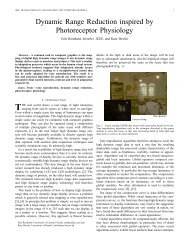
Our Universe of Discourse in this chapter will be the London Underground, of which a 

small part is shown in fig. 1.1. Note that this picture contains a wealth of information, 

about lines, stations, transit between lines, relative distance, etc. We will try to capture this 

information in logical statements. Basically, fig. 1.1 specifies which stations are directly 

connected by which lines. If we follow the lines from left to right (Northern downwards), we 

come up with the following 11 formulas: 

connected(bond_street,oxford_circus,central). 

connected(oxford_circus,tottenham_court_road,central). 

connected(bond_street,green_park,jubilee). 

connected(green_park,charing_cross,jubilee). 

connected(green_park,piccadilly_circus,piccadilly). 

connected(piccadilly_circus,leicester_square,piccadilly). 

connected(green_park,oxford_circus,victoria). 

connected(oxford_circus,piccadilly_circus,bakerloo). 

connected(piccadilly_circus,charing_cross,bakerloo). 

connected(tottenham_court_road,leicester_square,northern). 

connected(leicester_square,charing_cross,northern). 

Let’s define two stations to be nearby if they are on the same line, with at most one station 

in between. This relation can also be represented by a set of logical formulas: 

nearby(bond_street,oxford_circus). 

nearby(oxford_circus,tottenham_court_road). 

nearby(bond_street,tottenham_court_road). 

nearby(bond_street,green_park). 

nearby(green_park,charing_cross). 

nearby(bond_street,charing_cross).


JUBILEE BAKERLOO NORTHERN 

Bond 

Street 

UNDERGROUND 

Green 

Park 

Oxford 

Circus 

VICTORIA 

Piccadilly 

Circus 

Tottenham 

Court Road 

Charing 

Cross 

Leicester 

Square 

nearby(green_park,piccadilly_circus). 

nearby(piccadilly_circus,leicester_square). 

nearby(green_park,leicester_square). 

nearby(green_park,oxford_circus). 

nearby(oxford_circus,piccadilly_circus). 

nearby(piccadilly_circus,charing_cross). 

nearby(oxford_circus,charing_cross). 

nearby(tottenham_court_road,leicester_square). 

nearby(leicester_square,charing_cross). 

nearby(tottenham_court_road,charing_cross). 

CENTRAL 

These 16 formulas have been derived from the previous 11 formulas in a systematic way. If 

X and Y are directly connected via some line L, then X and Y are nearby. Alternatively, if 

there is some Z in between, such that X and Z are directly connected via L, and Z and Y are 

also directly connected via L, then X and Y are also nearby. We can formulate this in logic 

as follows: 

nearby(X,Y):-connected(X,Y,L). 

nearby(X,Y):-connected(X,Z,L),connected(Z,Y,L). 

PICCADILLY 

Figure 1.1. Part of the London Underground. Reproduced by permission 

of London Regional Transport (LRT Registered User No. 94/1954). 

In these formulas, the symbol ‘:-’ should be read as ‘if’, and the comma between 

connected(X,Z,L) and connected(Z,Y,L) should be read as ‘and’. The uppercase

1 Introduction to clausal logic 5 

letters stand for universally quantified variables, such that, for instance, the second formula 

means: 

For any values of X, Y, Z and L, X is nearby Y if X is directly connected to Z 

via L, and Z is directly connected to Y via L. 

We now have two definitions of the nearby-relation, one which simply lists all pairs of 

stations that are nearby each other, and one in terms of direct connections. Logical formulas 

of the first type, such as 

nearby(bond_street,oxford_circus) 

will be called facts, and formulas of the second type, such as 

nearby(X,Y):-connected(X,Z,L),connected(Z,Y,L) 

will be called rules. Facts express unconditional truths, while rules denote conditional truths, 

i.e. conclusions which can only be drawn when the premises are known to be true. 

Obviously, we want these two definitions to be equivalent: for each possible query, both 

definitions should give exactly the same answer. We will make this more precise in the next 

section. 

Exercise 1.1. Two stations are ‘not too far’ if they are on the same or a different 

line, with at most one station in between. Define rules for the predicate 

not_too_far. 

1.1 Answering queries 

A query like ‘which station is nearby Tottenham Court Road?’ will be written as 

?-nearby(tottenham_court_road,W) 

where the prefix ‘?-’ indicates that this is a query rather than a fact. An answer to this 

query, e.g. ‘Leicester Square’, will be written {W!leicester_square}, indicating a 

substitution of values for variables, such that the statement in the query, i.e. 

nearby(tottenham_court_road,leicester_square) 

is true. Now, if the nearby-relation is defined by means of a list of facts, answers to queries 

are easily found: just look for a fact that matches the query, by which is meant that the fact 

and the query can be made identical by substituting values for variables in the query. Once 

we have found such a fact, we also have the substitution which constitutes the answer to the 

query. 

If rules are involved, query-answering can take several of these steps. For answering the 

query ?-nearby(tottenham_court_road,W), we match it with the conclusion of 

the rule 

nearby(X,Y):-connected(X,Y,L)


?-nearby(tottenham_court_road,W) nearby(X,Y):-connected(X,Y,L) 

?-connected(tottenham_court_road,W,L) 

yielding the substitution {X!tottenham_court_road, Y!W}. We then try to find an 

answer for the premises of the rule under this substitution, i.e. we try to answer the query 

?-connected(tottenham_court_road,W,L). 

{X->tottenham_court_road, Y->W} 

connected(tottenham_court_road, 

leicester_square, 

northern) 

{W->leicester_square, L->northern} 

Figure 1.2. A proof tree for the query ?-nearby(tottenham_court_road,W). 

That is, we can find a station nearby Tottenham Court Road, if we can find a station directly 

connected to it. This second query is answered by looking at the facts for direct connections, 

giving the answer {W!leicester_square, L!northern}. Finally, since the 

variable L does not occur in the initial query, we just ignore it in the final answer, which 

becomes {W!leicester_square} as above. In fig. 1.2, we give a graphical 

representation of this process. Since we are essentially proving that a statement follows 

logically from some other statements, this graphical representation is called a proof tree. 

The steps in fig. 1.2 follow a very general reasoning pattern: 

to answer a query ?-Q1,Q2,…,Qn, find a rule A:-B1,…,Bm such that A 

matches with Q1, and answer the query ?-B1,…,Bm,Q2,…,Qn. 

This reasoning pattern is called resolution, and we will study it extensively in Chapters 2 

and 3. Resolution adds a procedural interpretation to logical formulas, besides their 

declarative interpretation (they can be either true or false). Due to this procedural 

interpretation, logic can be used as a programming language. In an ideal logic programming 

system, the procedural interpretation would exactly match the declarative interpretation: 

everything that is calculated procedurally is declaratively true, and vice versa. In such an ideal 

system, the programmer would just bother about the declarative interpretation of the 

formulas she writes down, and leave the procedural interpretation to the computer. 

Unfortunately, in current logic programming systems the procedural interpretation does not 

exactly match the declarative interpretation: for example, some things that are declaratively 

true are not calculated at all, because the system enters an infinite loop. Therefore, the 

programmer should also be aware of the procedural interpretation given by the computer to 

her logical formulas. 

The resolution proof process makes use of a technique that is known as reduction to the 

absurd: suppose that the formula to be proved is false, and show that this leads to a 

contradiction, thereby demonstrating that the formula to be proved is in fact true. Such a


proof is also called a proof by refutation. For instance, if we want to know which stations 

are nearby Tottenham Court Road, we negate this statement, resulting in ‘there are no 

stations nearby Tottenham Court Road’. In logic, this is achieved by writing the statement 

as a rule with an empty conclusion, i.e. a rule for which the truth of its premises would lead 

to falsity: 

:-nearby(tottenham_court_road,W) 

Thus, the symbols ‘?-’ and ‘:-’ are in fact equivalent. A contradiction is found if 

resolution leads to the empty rule, of which the premises are always true (since there are 

none), but the conclusion is always false. Conventionally, the empty rule is written as ‘ ’. 

At the beginning of this section, we posed the question: can we show that our two 

definitions of the nearby-relation are equivalent? As indicated before, the idea is that to be 

equivalent means to provide exactly the same answers to the same queries. To formalise this, 

we need some additional definitions. A ground fact is a fact without variables. Obviously, if 

G is a ground fact, the query ?-G never returns a substitution as answer: either it succeeds (G 

does follow from the initial assumptions), or it fails (G does not). The set of ground facts G 

for which the query ?-G succeeds is called the success set. Thus, the success set for our 

first definition of the nearby-relation consists simply of those 16 formulas, since they are 

ground facts already, and nothing else is derivable from them. The success set for the second 

definition of the nearby-relation is constructed by applying the two rules to the ground facts 

for connectedness. Thus we can say: two definitions of a relation are (procedurally) 

equivalent if they have the same success set (restricted to that relation). 

Exercise 1.2. Construct the proof trees for the query 

?-nearby(W,charing_cross). 

1.2 Recursion 

Until now, we have encountered two types of logical formulas: facts and rules. There is a 

special kind of rule which deserves special attention: the rule which defines a relation in 

terms of itself. This idea of ‘self-reference’, which is called recursion, is also present in most 

procedural programming languages. Recursion is a bit difficult to grasp, but once you’ve 

mastered it, you can use it to write very elegant programs, e.g. 

IF N=0 

THEN FAC:=1 

ELSE FAC:=N*FAC(N-1). 

is a recursive procedure for calculating the factorial of a given number, written in a Pascallike 

procedural language. However, in such languages iteration (looping a pre-specified 

number of times) is usually preferred over recursion, because it uses memory more 

efficiently.


In Prolog, however, recursion is the only looping structure 1 . (This does not 

necessarily mean that Prolog is always less efficient than a procedural language, because 

there are ways to write recursive loops that are just as efficient as iterative loops, as we will 

see in section 3.6.) Perhaps the easiest way to think about recursion is the following: an 

arbitrarily large chain is described by describing how one link in the chain is connected to 

the next. For instance, let us define the relation of reachability in our underground example, 

where a station is reachable from another station if they are connected by one or more lines. 

We could define it by the following 20 ground facts: 

reachable(bond_street,charing_cross). 

reachable(bond_street,green_park). 

reachable(bond_street,leicester_square). 

reachable(bond_street,oxford_circus). 

reachable(bond_street,piccadilly_circus). 

reachable(bond_street,tottenham_court_road). 

reachable(green_park,charing_cross). 

reachable(green_park,leicester_square). 

reachable(green_park,oxford_circus). 

reachable(green_park,piccadilly_circus). 

reachable(green_park,tottenham_court_road). 

reachable(leicester_square,charing_cross). 

reachable(oxford_circus,charing_cross). 

reachable(oxford_circus,leicester_square). 

reachable(oxford_circus,piccadilly_circus). 

reachable(oxford_circus,tottenham_court_road). 

reachable(piccadilly_circus,charing_cross). 

reachable(piccadilly_circus,leicester_square). 

reachable(tottenham_court_road,charing_cross). 

reachable(tottenham_court_road,leicester_square). 

Since any station is reachable from any other station by a route with at most two 

intermediate stations, we could instead use the following (non-recursive) definition: 

reachable(X,Y):- connected(X,Y,L). 

reachable(X,Y):- connected(X,Z,L1),connected(Z,Y,L2). 

reachable(X,Y):- connected(X,Z1,L1),connected(Z1,Z2,L2), 

connected(Z2,Y,L3). 

Of course, if we were to define the reachability relation for the entire London underground, 

we would need a lot more, longer and longer rules. Recursion is a much more convenient 

and natural way to define such chains of arbitrary length: 

reachable(X,Y):-connected(X,Y,L). 

reachable(X,Y):-connected(X,Z,L),reachable(Z,Y). 

The reading of the second rule is as follows: ‘Y is reachable from X if Z is directly connected 

to X via line L, and Y is reachable from Z’. 

1 If we take Prolog’s procedural behaviour into account, there are alternatives to recursive 

loops such as the so-called failure-driven loop (see Exercise 7.5).


:-reachable(bond_street,W) reachable(X,Y):-connected(X,Z,L), 

reachable(Z,Y) 

:-connected(bond_street,Z,L), 

reachable(Z,W) 

We can now use this recursive definition to prove that Leicester Square is reachable 

from Bond Street (fig. 1.3). However, just as there are several routes from Bond Street to 

Leicester Square, there are several alternative proofs of the fact that Leicester Square is 

reachable from Bond Street. An alternative proof is given in fig. 1.4. The difference between 

these two proofs is that in the first proof we use the fact 

connected(oxford_circus,tottenham_court_road,central) 

while in the second proof we use 

{X->bond_street, Y->W} 

connected(bond_street, 

oxford_circus, 

central) 

{Z->oxford_circus, L->central} 

:-reachable(oxford_circus,W) reachable(X,Y):-connected(X,Z,L), 


:-connected(oxford_circus,Z,L), 


{X->oxford_circus, Y->W} 

connected(oxford_circus, 

tottenham_court_road, 

central) 

{Z->tottenham_court_road, L->central} 

:-reachable(tottenham_court_road,W) reachable(X,Y):-connected(X,Y,L) 


:-connected(tottenham_court_road,W,L) connected(tottenham_court_road, 


northern) 

{W->leicester_square, L->northern} 

Figure 1.3. A proof tree for the query ?-reachable(bond_street,W). 

connected(oxford_circus,piccadilly_circus,bakerloo) 

There is no reason to prefer one over the other, but since Prolog searches the given formulas 

top-down, it will find the first proof before the second. Thus, the order of the clauses 

determines the order in which answers are found. As we will see in Chapter 3, it sometimes 

even determines whether any answers are found at all.


:-reachable(bond_street,W) reachable(X,Y):-connected(X,Z,L), 


:-connected(bond_street,Z,L), 


{X->bond_street, Y->W} 

connected(bond_street, 

oxford_circus, 

central) 

{Z->oxford_circus, L->central} 

:-reachable(oxford_circus,W) reachable(X,Y):-connected(X,Z,L), 


:-connected(oxford_circus,Z,L), 


{X->oxford_circus, Y->W} 

connected(oxford_circus, 

piccadilly_circus, 

bakerloo) 

{Z->piccadilly_circus, L->bakerloo} 

:-reachable(piccadilly_circus,W) reachable(X,Y):-connected(X,Y,L) 

:-connected(piccadilly_circus,W,L) 

{X->piccadilly_circus, Y->W} 

connected(piccadilly_circus, 


piccadilly) 

{W->leicester_square, L->piccadilly} 

Figure 1.4. Alternative proof tree for the query ?reachable(bond_street,W). 

Exercise 1.3. Give a third proof tree for the answer {W!leicester_square}, and 

change the order of the facts for connectedness, such that this proof tree is 

constructed first. 

In other words, Prolog’s query-answering process is a search process, in which the 

answer depends on all the choices made earlier. A important point is that some of these 

choices may lead to a dead-end later. For example, if the recursive formula for the 

reachability relation had been tried before the non-recursive one, the bottom part of fig. 1.3 

would have been as in fig. 1.5. This proof tree cannot be completed, because there are no 

answers to the query ?-reachable(charing_cross,W), as can easily be checked.

:-reachable(tottenham_court_road,W) 

:-connected(tottenham_court_road,Z,L), 


:-reachable(leicester_square,W) 

:-connected(leicester_square,Z,L), 


:-reachable(charing_cross,W) 


Prolog has to recover from this failure by climbing up the tree, reconsidering previous 

choices. This search process, which is called backtracking, will be detailed in Chapter 5. 

1.3 Structured terms 

reachable(X,Y):-connected(X,Z,L), 



connected(tottenham_court_road, 


northern) 

{Z->leicester_square, L->northern} 

{X->leicester_square, Y->W} 

{Z->charing_cross, L->northern} 

Figure 1.5. A failing proof tree. 

reachable(X,Y):-connected(X,Z,L), 


Finally, we illustrate the way Prolog can handle more complex datastructures, such as a list 

of stations representing a route. Suppose we want to redefine the reachability relation, such 

that it also specifies the intermediate stations. We could adapt the non-recursive definition of 

reachable as follows: 

reachable0(X,Y):-connected(X,Y,L). 

reachable1(X,Y,Z):- connected(X,Z,L1), 

connected(Z,Y,L2). 

reachable2(X,Y,Z1,Z2):- connected(X,Z1,L1), 

connected(Z1,Z2,L2), 


connected(leicester_square, 

charing_cross, 

northern) 

The suffix of reachable indicates the number of intermediate stations; it is added to stress that 

relations with different number of arguments are really different relations, even if their names 

are the same. The problem now is that we have to know the number of intermediate stations 

in advance, before we can ask the right query. This is, of course, unacceptable. 

We can solve this problem by means of functors. A functor looks just like a 

mathematical function, but the important difference is that functor expressions are never


route 

tottenham_court_road 

leicester_square 

route 

Figure 1.6. A complex object as a tree. 

evaluated to determine a value. Instead, they provide a way to name a complex object 

composed of simpler objects. For instance, a route with Oxford Circus and Tottenham Court 

Road as intermediate stations could be represented by 

route(oxford_circus,tottenham_court_road) 

noroute 

Note that this is not a ground fact, but rather an argument for a logical formula. The 

reachability relation can now be defined as follows: 

reachable(X,Y,noroute):-connected(X,Y,L). 

reachable(X,Y,route(Z)):- connected(X,Z,L1), 

connected(Z,Y,L2). 

reachable(X,Y,route(Z1,Z2)):- connected(X,Z1,L1), 

connected(Z1,Z2,L2), 


The query ?-reachable(oxford_circus,charing_cross,R) now has three 

possible answers: 

{R!route(piccadilly_circus)} 

{R!route(tottenham_court_road,leicester_square)} 

{R!route(piccadilly_circus,leicester_square)} 

As argued in the previous section, we prefer the recursive definition of the reachability 

relation, in which case we use functors in a somewhat different way. 

reachable(X,Y,noroute):-connected(X,Y,L). 

reachable(X,Y,route(Z,R)):- connected(X,Z,L), 

reachable(Z,Y,R). 

At first sight, there does not seem to be a big difference between this and the use of functors 

in the non-recursive program. However, the query


?-reachable(oxford_circus,charing_cross,R) 

now has the following answers: 

a 

. 

{R!route(tottenham_court_road, 

route(leicester_square,noroute))} 

{R!route(piccadilly_circus,noroute)} 

{R!route(piccadilly_circus, 

route(leicester_square,noroute))} 

The functor route is now also recursive in nature: its first argument is a station, but its 

second argument is again a route. For instance, the object 

route(tottenham_court_road,route(leicester_square,noroute)) 

can be pictured as in fig. 1.6. Such a figure is called a tree (we will have a lot more to say 

about trees in chapter 4). In order to find out the route represented by this complex object, 

we read the leaves of this tree from left to right, until we reach the ‘terminator’ noroute. 

This would result in a linear notation like 

[tottenham_court_road,leicester_square]. 

b 

. 

Figure 1.7. The list [a,b,c] as a tree. 

For user-defined functors, such a linear notation is not available. However, Prolog 

provides a built-in ‘datatype’ called lists, for which both the tree-like notation and the linear 

notation may be used. The functor for lists is . (dot), which takes two arguments: the first 

element of the list (which may be any object), and the rest of the list (which must be a list). 

The list terminator is the special symbol [], denoting the empty list. For instance, the term 

c 

. 

[]


.(a,.(b,.(c,[]))) 

denotes the list consisting of a followed by b followed by c (fig. 1.7). Alternatively, we 

may use the linear notation, which uses square brackets: 

[a,b,c] 

To increase readability of the tree-like notation, instead of 

.(First,Rest) 

one can also write 

[First|Rest] 

Note that Rest is a list: e.g., [a,b,c] is the same list as [a|[b,c]]. a is called the 

head of the list, and [b,c] is called its tail. Finally, to a certain extent the two notations 

can be mixed: at the head of the list, you can write any number of elements in linear 

notation. For instance, 

[First,Second,Third|Rest] 

denotes a list with three or more elements. 

Exercise 1.4. A list is either the empty list [], or a non-empty list [First|Rest] 

where Rest is a list. Define a relation list(L), which checks whether L is a list. 

Adapt it such that it succeeds only for lists of (i) even length and (ii) odd length. 

The recursive nature of such datastructures makes it possible to ignore the size of the 

objects, which is extremely useful in many situations. For instance, the definition of a route 

between two underground stations does not depend on the length of the route; all that matters 

is whether there is an intermediate station or not. For both cases, there is a clause. 

Expressing the route as a list, we can state the final definition of the reachability relation: 

reachable(X,Y,[]):-connected(X,Y,L). 

reachable(X,Y,[Z|R]):-connected(X,Z,L),reachable(Z,Y,R). 

The query ?-reachable(oxford_circus,charing_cross,R) now results in the 

following answers: 

{R![tottenham_court_road,leicester_square]} 

{R![piccadilly_circus]} 

{R![piccadilly_circus, leicester_square]} 

Note that Prolog writes out lists of fixed length in the linear notation. 

Should we for some reason want to know from which station Charing Cross can be 

reached via a route with four intermediate stations, we should ask the query 

?-reachable(X,charing_cross,[A,B,C,D]) 

which results in two answers:


{ X!bond_street, A!green_park, B!oxford_circus, 

C!tottenham_court_road, D!leicester_square } 

{ X!bond_street, A!green_park, B!oxford_circus, 

C!piccadilly_circus, D!leicester_square }. 

Exercise 1.5. Construct a query asking for a route from Bond Street to Piccadilly 

Circus with at least two intermediate stations. 

1.4 What else is there to know about clausal logic? 

The main goal of this chapter has been to introduce the most important concepts in clausal 

logic, and how it can be used as a reasoning formalism. Needless to say, a subject like this 

needs a much more extensive and precise discussion than has been attempted here, and many 

important questions remain. To name a few: 

• what are the limits of expressiveness of clausal logic, i.e. what can and what 

cannot be expressed? 

• what are the limits of reasoning with clausal logic, i.e. what can and what 

cannot be (efficiently) computed? 

• how are these two limits related: is it for instance possible to enhance 

reasoning by limiting expressiveness? 

In order to start answering such questions, we need to be more precise in defining what 

clausal logic is, what expressions in clausal logic mean, and how we can reason with them. 

That means that we will have to introduce some theory in the next chapter. This theory will 

not only be useful for a better understanding of Logic Programming, but it will also be the 

foundation for most of the topics in Part III (Advanced reasoning techniques). 

Another aim of Part I of this book is to teach the skill of programming in Prolog. For 

this, theory alone, however important, will not suffice. Like any programming language, 

Prolog has a number of built-in procedures and datastructures that you should know about. 

Furthermore, there are of course numerous programming techniques and tricks of the trade, 

with which the Prolog programmer should be familiar. These subjects will be discussed in 

Chapter 3. Together, Chapters 2 and 3 will provide a solid foundation for the rest of the 

book.

2 

Clausal logic and resolution: 

theoretical backgrounds 

In this chapter we develop a more formal view of Logic Programming by means of a 

rigorous treatment of clausal logic and resolution theorem proving. Any such treatment has 

three parts: syntax, semantics, and proof theory. Syntax defines the logical language we are 

using, i.e. the alphabet, different kinds of ‘words’, and the allowed ‘sentences’. Semantics 

defines, in some formal way, the meaning of words and sentences in the language. As with 

most logics, semantics for clausal logic is truth-functional, i.e. the meaning of a sentence is 

defined by specifying the conditions under which it is assigned certain truth values (in our 

case: true or false). Finally, proof theory specifies how we can obtain new sentences 

(theorems) from assumed ones (axioms) by means of pure symbol manipulation (inference 

rules). 

Of these three, proof theory is most closely related to Logic Programming, because 

answering queries is in fact no different from proving theorems. In addition to proof theory, 

we need semantics for deciding whether the things we prove actually make sense. For 

instance, we need to be sure that the truth of the theorems is assured by the truth of the 

axioms. If our inference rules guarantee this, they are said to be sound. But this will not be 

enough, because sound inference rules can be actually very weak, and unable to prove 

anything of interest. We also need to be sure that the inference rules are powerful enough to 

eventually prove any possible theorem: they should be complete. 

Concepts like soundness and completeness are called meta-theoretical, since they are not 

expressed in the logic under discussion, but rather belong to a theory about that logic 

(‘meta’ means above). Their significance is not merely theoretical, but extends to logic 

programming languages like Prolog. For example, if a logic programming language is 

unsound, it will give wrong answers to some queries; if it is incomplete, it will give no 

answer to some other queries. Ideally, a logic programming language should be sound and 

complete; in practice, this will not be the case. For instance, in the next chapter we will see 

that Prolog is both unsound and incomplete. This has been a deliberate design choice: a 

sound and complete Prolog would be much less efficient. Nevertheless, any Prolog 

programmer should know exactly the circumstances under which Prolog is unsound or 

incomplete, and avoid these circumstances in her programs.


The structure of this chapter is as follows. We start with a very simple (propositional) 

logical language, and enrich this language in two steps to full clausal logic. For each of 

these three languages, we discuss syntax, semantics, proof theory, and meta-theory. We then 

discuss definite clause logic, which is the subset of clausal logic used in Prolog. Finally, we 

relate clausal logic to Predicate Logic, and show that they are essentially equal in expressive 

power. 

2.1 Propositional clausal logic 

Informally, a proposition is any statement which is either true or false, such as ‘2 + 2 = 4’ 

or ‘the moon is made of green cheese’. These are the building blocks of propositional logic, 

the weakest form of logic. 

Syntax. Propositions are abstractly denoted by atoms, which are single words starting with 

a lowercase character. For instance, married is an atom denoting the proposition ‘he/she 

is married’; similarly, man denotes the proposition ‘he is a man’. Using the special symbols 

‘:-’ (if), ‘;’ (or) and ‘,’ (and), we can combine atoms to form clauses. For instance, 

married;bachelor:-man,adult 

is a clause, with intended meaning: ‘somebody is married or a bachelor if he is a man and 

an adult’ 2 . The part to the left of the if-symbol ‘:-’ is called the head of the clause, and the 

right part is called the body of the clause. The head of a clause is always a disjunction (or) 

of atoms, and the body of a clause is always a conjunction (and). 

Exercise 2.1. Translate the following statements into clauses, using the atoms 

person, sad and happy: 

(a) persons are happy or sad; 

(b) no person is both happy and sad; 

(c) sad persons are not happy; 

(d) non-happy persons are sad. 

A program is a set of clauses, each of them terminated by a period. The clauses are to be 

read conjunctively; for example, the program 

woman;man:-human. 

human:-woman. 

human:-man. 

has the intended meaning ‘(if someone is human then she/he is a woman or a man) and 

(if someone is a woman then she is human) and (if someone is a man then he is 

human)’, or, in other words, ‘someone is human if and only if she/he is a woman or a 

man’. 

2 It is often more convenient to read a clause in the opposite direction: 

‘if somebody is a man and an adult then he is married or a bachelor’.

2 Theoretical backgrounds 19 

Semantics. The Herbrand base of a program P is the set of atoms occurring in P. For the 

above program, the Herbrand base is {woman, man, human}. A Herbrand interpretation (or 

interpretation for short) for P is a mapping from the Herbrand base of P into the set of truth 

values {true, false}. For example, the mapping {woman!true, man!false, 

human!true} is a Herbrand interpretation for the above program. A Herbrand 

interpretation can be viewed as describing a possible state of affairs in the Universe of 

Discourse (in this case: ‘she is a woman, she is not a man, she is human’). Since there are 

only two possible truth values in the semantics we are considering, we could abbreviate such 

mappings by listing only the atoms that are assigned the truth value true; by definition, the 

remaining ones are assigned the truth value false. Under this convention, which we will 

adopt in this book, a Herbrand interpretation is simply a subset of the Herbrand base. Thus, 

the previous Herbrand interpretation would be represented as {woman, human}. 

Since a Herbrand interpretation assigns truth values to every atom in a clause, it also 

assigns a truth value to the clause as a whole. The rules for determining the truth value of a 

clause from the truth values of its atoms are not so complicated, if you keep in mind that 

the body of a clause is a conjunction of atoms, and the head is a disjunction. Consequently, 

the body of a clause is true if every atom in it is true, and the head of a clause is true if at 

least one atom in it is true. In turn, the truth value of the clause is determined by the truth 

values of head and body. There are four possibilities: 

(i) the body is true, and the head is true; 

(ii) the body is true, and the head is false; 

(iii) the body is false, and the head is true; 

(iv) the body is false, and the head is false. 

The intended meaning of the clause is ‘if body then head’, which is obviously true in the 

first case, and false in the second case. 

What about the remaining two cases? They cover statements like ‘if the moon is made 

of green cheese then 2 + 2 = 4’, in which there is no connection at all between body and 

head. One would like to say that such statements are neither true nor false. However, our 

semantics is not sophisticated enough to deal with this: it simply insists that clauses should 

be assigned a truth value in every possible interpretation. Therefore, we consider the clause 

to be true whenever its body is false. It is not difficult to see that under these truth 

conditions a clause is equivalent with the statement ‘head or not body’. For example, the 

clause married;bachelor:-man,adult can also be read as ‘someone is married or a 

bachelor or not a man or not an adult’. Thus, a clause is a disjunction of atoms, which are 

negated if they occur in the body of the clause. Therefore, the atoms in the body of the 

clause are often called negative literals, while those in the head of the clause are called 

positive literals. 

To summarise: a clause is assigned the truth value true in an interpretation, if and only 

if at least one of the following conditions is true: (a) at least one atom in the body of the 

clause is false in the interpretation (cases (iii) and (iv)), or (b) at least one atom in the head 

of the clause is true in the interpretation (cases (i) and (iii)). If a clause is true in an 

interpretation, we say that the interpretation is a model for the clause. An interpretation is a 

model for a program if it is a model for each clause in the program. For example, the above 

program has the following models: " (the empty model, assigning false to every atom), 

{woman, human}, {man, human}, and {woman, man, human}. Since there are eight


possible interpretations for a Herbrand base with three atoms, this means that the program 

contains enough information to rule out half of these. 

Adding more clauses to the program means restricting its set of models. For instance, if 

we add the clause woman (a clause with an empty body) to the program, we rule out the first 

and third model, which leaves us with the models {woman, human}, and {woman, man, 

human}. Note that in both of these models, human is true. We say that human is a 

logical consequence of the set of clauses. In general, a clause C is a logical consequence of a 

program P if every model of the program is also a model of the clause; we write P C. 

Exercise 2.2. Given the program 

married;bachelor:-man,adult. 

man. 

:-bachelor. 

determine which of the following clauses are logical consequences of this program: 

(a) married:-adult; 

(b) married:-bachelor; 

(c) bachelor:-man; 

(d) bachelor:-bachelor. 

Of the two remaining models, obviously {woman, human} is the intended one; but the 

program does not yet contain enough information to distinguish it from the non-intended 

model {woman, man, human}. We can add yet another clause, to make sure that the atom 

man is mapped to false. For instance, we could add 

:-man 

(it is not a man) or 

:-man,woman 

(nobody is both a man and a woman). However, explicitly stating everything that is false in 

the intended model is not always feasible. Consider, for example, an airline database 

consulted by travel agencies: we simply want to say that if a particular flight (i.e., a 

combination of plane, origin, destination, date and time) is not listed in the database, then it 

does not exist, instead of listing all the dates that a particular plane does not fly from 

Amsterdam to London. 

So, instead of adding clauses until a single model remains, we want to add a rule to our 

semantics which tells us which of the several models is the intended one. The airline 

example shows us that, in general, we only want to accept something as true if we are 

really forced to, i.e. if it is true in every possible model. This means that we should take 

the intersection of every model of a program in order to construct the intended model. In the 

example, this is {woman, human}. Note that this model is minimal in the sense that no 

subset of it is also a model. Therefore, this semantics is called a minimal model semantics. 

Unfortunately, this approach is only applicable to a restricted class of programs. 

Consider the following program:

woman;man:-human. 

human. 


This program has three models: {woman, human}, {man, human}, and {woman, man, 

human}. The intersection of these models is {human}, but this interpretation is not a 

model of the first clause! The program has in fact not one, but two minimal models, which 

is caused by the fact that the first clause has a disjunctive head. Such a clause is called 

indefinite, because it does not permit definite conclusions to be drawn. 

On the other hand, if we would only allow definite clauses, i.e. clauses with a single 

positive literal, minimal models are guaranteed to be unique. We will deal with definite 

clauses in section 2.4, because Prolog is based on definite clause logic. In principle, this 

means that clauses like woman;man:-human are not expressible in Prolog. However, 

such a clause can be transformed into a ‘pseudo-definite’ clause by moving one of the literals 

in the head to the body, extended with an extra negation. This gives the following two 

possibilities: 

woman:-human,not(man). 

man:-human,not(woman). 

In Prolog, we have to choose between these two clauses, which means that we have only an 

approximation of the original indefinite clause. Negation in Prolog is an important subject 

with many aspects. In Chapter 3, we will show how Prolog handles negation in the body of 

clauses. In Chapter 8, we will discuss particular applications of this kind of negation. 

Proof theory. Recall that a clause C is a logical consequence of a program P (P C) if 

every model of P is a model of C. Checking this condition is, in general, unfeasible. 

Therefore, we need a more efficient way of computing logical consequences, by means of 

inference rules. If C can be derived from P by means of a number of applications of such 

inference rules, we say that C can be proved from P. Such inference rules are purely 

syntactic, and do not refer to any underlying semantics. 

The proof theory for clausal logic consists of a single inference rule called resolution. 

Resolution is a very powerful inference rule. Consider the following program: 


has_wife:-man,married. 

This simple program has no less than 26 models, each of which needs to be considered if we 

want to check whether a clause is a logical consequence of it. 

Exercise 2.3. Write down the six Herbrand interpretations that are not models of 

the program. 

The following clause is a logical consequence of this program: 

has_wife;bachelor:-man,adult 

By means of resolution, it can be produced in a single step. This step represents the 

following line of reasoning: ‘if someone is a man and an adult, then he is a bachelor or


has_wife:-man,married married;bachelor:-man,adult 

married; but if he is married, he has a wife; therefore, if someone is a man and an adult, then 

he is a bachelor or he has a wife’. In this argument, the two clauses in the program are 

related to each other by means of the atom married, which occurs in the head of the first 

clause (a positive literal) and in the body of the second (a negative literal). The derived 

clause, which is called the resolvent, consists of all the literals of the two input clauses, 

except married (the literal resolved upon). The negative literal man, which occurs in both 

input clauses, appears only once in the derived clause. This process is depicted in fig. 2.1. 

Resolution is most easily understood when applied to definite clauses. Consider the 

following program: 

square:-rectangle,equal_sides. 

rectangle:-parallelogram,right_angles. 

Applying resolution yields the clause 

has_wife;bachelor:-man,adult 

Figure 2.1. A resolution step. 

square:-parallelogram,right_angles,equal_sides 

That is, the atom rectangle in the body of the first clause is replaced by the body of the 

second clause (which has rectangle as its head). This process is also referred to as 

unfolding the second clause into the first one (fig. 2.2). 

A resolvent resulting from one resolution step can be used as input for the next. A 

proof or derivation of a clause C from a program P is a sequence of clauses such that each 

square:-rectangle,equal_sides rectangle:-parallelogram,right_angles 

square:-parallelogram,right_angles,equal_sides 

Figure 2.2. Resolution with definite clauses.


clause is either in the program, or the resolvent of two previous clauses, and the last clause 

is C. If there is a proof of C from P, we write P C. 

Exercise 2.4. Give a derivation of friendly from the following program: 

happy;friendly:-teacher. 

friendly:-teacher,happy. 

teacher;wise. 

teacher:-wise. 

Meta-theory. It is easy to show that propositional resolution is sound: you have to 

establish that every model for the two input clauses is a model for the resolvent. In our 

earlier example, every model of married;bachelor:-man,adult and has_wife:man,married 

must be a model of has_wife;bachelor:-man,adult. Now, the 

literal resolved upon (in this case married) either assigned the truth value true or 

false. In the first case, every model of has_wife:-man,married is also a model of 

has_wife:-man; in the second case, every model of married;bachelor:man,adult 

is also a model of bachelor:-man,adult. In both cases, these models 

are models of a subclause of the resolvent, which means that they are also models of the 

resolvent itself. 

In general, proving completeness is more complicated than proving soundness. Still 

worse, proving completeness of resolution is impossible, because resolution is not complete 

at all! For instance, consider the clause a:-a. This clause is a so-called tautology: it is true 

under any interpretation. Therefore, any model of an arbitrary program P is a model for it, 

and thus P a:-a for any program P. If resolution were complete, it would be possible to 

derive the clause a:-a from some program P in which the literal a doesn’t even occur! It is 

clear that resolution is unable to do this. 

However, this is not necessarily bad, because although tautologies follow from any set 

of clauses, they are not very interesting. Resolution makes it possible to guide the inference 

process, by implementing the question ‘is C a logical consequence of P?’ rather than ‘what 

are the logical consequences of P?’. We will see that, although resolution is unable to 

generate every logical consequence of a set of clauses, it is complete in the sense that 

resolution can always determine whether a specific clause is a logical consequence of a set of 

clauses. 

The idea is analogous to a proof technique in mathematics called ‘reduction to the 

absurd’. Suppose for the moment that C consists of a single positive literal a; we want to 

know whether P a, i.e. whether every model of P is also a model of a. It is easily 

checked that an interpretation is a model of a if, and only if, it is not a model of :-a. 

Therefore, every model of P is a model of a if, and only if, there is no interpretation which 

is a model of both :-a and P. In other words, a is a logical consequence of P if, and only 

if, :-a and P are mutually inconsistent (don’t have a common model). So, checking 

whether P a is equivalent to checking whether P #{:-a} is inconsistent. 

Resolution provides a way to check this condition. Note that, since an inconsistent set 

of clauses doesn’t have a model, it trivially satisfies the condition that any model of it is a 

model of any other clause; therefore, an inconsistent set of clauses has every possible clause


as its logical consequence. In particular, the absurd or empty clause, denoted by 3 , is a 

logical consequence of an inconsistent set of clauses. Conversely, if is a logical 

consequence of a set of clauses, we know it must be inconsistent. Now, resolution is 

complete in the sense that if P set of clauses is inconsistent, it is always possible to derive 

by resolution. Since resolution is sound, we already know that if we can derive then 

the input clauses must be inconsistent. So we conclude: a is a logical consequence of P if, 

and only if, the empty clause can be deduced by resolution from P augmented with :-a. 

This process is called proof by refutation, and resolution is called refutation complete. 

This proof method can be generalised to the case where B is not a single atom. For 

instance, let us check by resolution that a:-a is a tautology, i.e. a logical consequence of 

any set of clauses. Logically speaking, this clause is equivalent to ‘a or not a’, the 

negation of which is ‘not a and a’, which is represented by two separate clauses :-a and 

a. Since we can derive the empty clause from these two clauses in a single resolution step 

without using any other clauses, we have in fact proved that a:-a is a logical consequence 

of an empty set of clauses, hence a tautology. 

Exercise 2.5. Prove by refutation that friendly:-has_friends is a logical 

consequence of the following clauses: 

happy:-has_friends. 

friendly:-happy. 

Finally, we mention that although resolution can always be used to prove inconsistency 

of a set of clauses it is not always fit to prove the opposite, i.e. consistency of a set of 

clauses. For instance, a is not a logical consequence of a:-a; yet, if we try to prove the 

inconsistency of :-a and a:-a (which should fail) we can go on applying resolution 

forever! The reason, of course, is that there is a loop in the system: applying resolution to 

:-a and a:-a again yields :-a. In this simple case it is easy to check for loops: just 

maintain a list of previously derived clauses, and do not proceed with clauses that have been 

derived previously. 

However, as we will see, this is not possible in the general case of full clausal logic, 

which is semi-decidable with respect to the question ‘is B a logical consequence of A’: there 

is an algorithm which derives, in finite time, a proof if one exists, but there is no algorithm 

which, for any A and B, halts and returns ‘no’ if no proof exists. The reason for this is that 

interpretations for full clausal logic are in general infinite. As a consequence, some Prolog 

programs may loop forever (just like some Pascal programs). One might suggest that it 

should be possible to check, just by examining the source code, whether a program is going 

to loop or not, but, as Alan Turing showed, this is, in general, impossible (the Halting 

Problem). That is, you can write programs for checking termination of programs, but for 

any such termination checking program you can write a program on which it will not 

terminate itself! 

3 is called the empty clause because it has empty body and head, and therefore it is not 

satisfiable by any interpretation.

2.2 Relational clausal logic 


Propositional clausal logic is rather coarse-grained, because it takes propositions (i.e. 

anything that can be assigned a truth value) as its basic building blocks. For example, it is 

not possible to formulate the following argument in propositional logic: 

Peter likes all his students 

Maria is one of Peter’s students 

Therefore, Peter likes Maria 

In order to formalise this type of reasoning, we need to talk about individuals like Peter and 

Maria, sets of individuals like Peter’s students, and relations between individuals, such as 

‘likes’. This refinement of propositional clausal logic leads us into relational clausal logic. 

Syntax. Individual names are called constants; we follow the Prolog convention of writing 

them as single words starting with a lowercase character (or as arbitrary strings enclosed in 

single quotes, like 'this is a constant'). Arbitrary individuals are denoted by 

variables, which are single words starting with an uppercase character. Jointly, constants and 

variables are denoted as terms. A ground term is a term without variables 4 . 

Relations between individuals are abstractly denoted by predicates (which follow the 

same notational conventions as constants). An atom is a predicate followed by a number of 

terms, enclosed in brackets and separated by commas, e.g. likes(peter,maria). The 

terms between brackets are called the arguments of the predicate, and the number of 

arguments is the predicate’s arity. The arity of a predicate is assumed to be fixed, and 

predicates with the same name but different arity are assumed to be different. A ground atom 

is an atom without variables. 

All the remaining definitions pertaining to the syntax of propositional clausal logic, in 

particular those of literal, clause and program, stay the same. So, the following clauses are 

meant to represent the above statements: 

likes(peter,S):-student_of(S,peter). 

student_of(maria,peter). 

likes(peter,maria). 

The intended meaning of these clauses are, respectively, ‘if S is a student of Peter then 

Peter likes S’, ‘Maria is a student of Peter’, and ‘Peter likes Maria’. Clearly, we want our 

logic to be such that the third clause follows logically from the first two, and we want to be 

able to prove this by resolution. Therefore, we must extend the semantics and proof theory 

in order to deal with variables. 

Semantics. The Herbrand universe of a program P is the set of ground terms (i.e. 

constants) occurring in it. For the above program, the Herbrand universe is {peter, 

maria}. The Herbrand universe is the set of all individuals we are talking about in our 

clauses. The Herbrand base of P is the set of ground atoms that can be constructed using 

the predicates in P and the ground terms in the Herbrand universe. This set represents all the 

things we can say about the individuals in the Herbrand universe. 

4 In relational clausal logic, ground terms are necessarily constants. However, this is not 

the case in full clausal logic, as we will see in section 2.3.


The Herbrand base of the above program is 

{ likes(peter,peter), likes(peter,maria), 

likes(maria,peter), likes(maria,maria), 

student_of(peter,peter), student_of(peter,maria), 

student_of(maria,peter), student_of(maria,maria) } 

As before, a Herbrand interpretation is the subset of the Herbrand base whose elements are 

assigned the truth value true. For instance, 

{likes(peter,maria), student_of(maria,peter)} 

is an interpretation of the above program. 

Clearly, we want this interpretation to be a model of the program, but now we have to 

deal with the variables in the program. A substitution is a mapping from variables to terms. 

For example, {S!maria} and {S!X} are substitutions. A substitution can be applied to a 

clause, which means that all occurrences of a variable occurring on the lefthand side in a 

substitution are replaced by the term on the righthand side. For instance, if C is the clause 

likes(peter,S):-student_of(S,peter) 

then the above substitutions yield the clauses 

Logical variables 

Variables in clausal logic are very similar to variables in mathematical formulas: 

they are placeholders that can be substituted by arbitrary ground terms from the 

Herbrand universe. It is very important to notice that logical variables are global 

within a clause (i.e. if the variable occurs at several positions within a clause, it 

should be substituted everywhere by the same term), but not within a program. This 

can be clearly seen from the semantics of relational clausal logic, where grounding 

substitutions are applied to clauses rather than programs. As a consequence, 

variables in two different clauses are distinct by definition, 

even if they have the same name. It will sometimes be useful to rename the 

variables in clauses, such that no two clauses share a variable; this is called 

standardising the clauses apart. 

likes(peter,maria):-student_of(maria,peter) 

likes(peter,X):-student_of(X,peter) 

Notice that the first clause is ground; it is said to be a ground instance of C, and the 

substitution {S!maria} is called a grounding substitution. All the atoms in a ground 

clause occur in the Herbrand base, so reasoning with ground clauses is just like reasoning 

with propositional clauses. An interpretation is a model for a non-ground clause if it is a 

model for every ground instance of the clause. Thus, in order to show that 

M = {likes(peter,maria), student_of(maria,peter)}


is a model of the clause C above, we have to construct the set of the ground instances of C 

over the Herbrand universe {peter, maria}, which is 

{ likes(peter,maria):-student_of(maria,peter), 

likes(peter,peter):-student_of(peter,peter) } 

and show that M is a model of every element of this set. 

Exercise 2.6. How many models does C have over the Herbrand universe 

{peter, maria}? 

Proof theory. Because reasoning with ground clauses is just like reasoning with 

propositional clauses, a naive proof method in relational clausal logic would apply 

grounding substitutions to every clause in the program before applying resolution. Such a 

method is naive, because a program has many different grounding substitutions, most of 

which do not lead to a resolution proof. For instance, if the Herbrand universe contains four 

constants, then a clause with two distinct variables has 16 different grounding substitutions, 

and a program consisting of three such clauses has 4096 different grounding substitutions. 

Instead of applying arbitrary grounding substitutions before trying to apply resolution, 

we will derive the required substitutions from the clauses themselves. Recall that in order to 

apply propositional resolution, the literal resolved upon should occur in both input clauses 

(positive in one clause and negative in the other). In relational clausal logic, atoms can 

contain variables. Therefore, we do not require that exactly the same atom occurs in both 

clauses; rather, we require that there is a pair of atoms which can be made equal by 

substituting terms for variables. For instance, let P be the following program: 


student_of(maria,T):-follows(maria,C),teaches(T,C). 

The second clause is intended to mean: ‘Maria is a student of any teacher who teaches a 

course she follows’. From these two clauses we should be able to prove that ‘Peter likes 

Maria if Maria follows a course taught by Peter’. This means that we want to resolve the 

two clauses on the student_of literals. 

The two atoms student_of(S,peter) and student_of(maria,T) can be 

made equal by replacing S by maria and T by peter, by means of the substitution 

{S!maria, T!peter}. This process is called unification, and the substitution is called a 

unifier. Applying this substitution yields the following two clauses: 

likes(peter,maria):-student_of(maria,peter). 

student_of(maria,peter):-follows(maria,C), 

teaches(peter,C). 

(Note that the second clause is not ground.) We can now construct the resolvent in the usual 

way, by dropping the literal resolved upon and combining the remaining literals, which 

yields the required clause 

likes(peter,maria):-follows(maria,C),teaches(peter,C)


Exercise 2.7. Write a clause expressing that Peter teaches all the first-year courses, 

and apply resolution to this clause and the above resolvent. 

Consider the following two-clause program P$: 


student_of(X,T):-follows(X,C),teaches(T,C). 

which differs from the previous program P in that the constant maria in the second clause 

has been replaced by a variable. Since this generalises the applicability of this clause from 

Maria to any of Peter’s students, it follows that any model for P$ over a Herbrand universe 

including maria is also a model for P, and therefore P$ P. In particular, this means that 

all the logical consequences of P$ are also logical consequences of P. For instance, we can 

again derive the clause 

likes(peter,maria):-follows(maria,C),teaches(peter,C) 

from P$ by means of the unifier {S!maria, X!maria, T!peter}. 

Unifiers are not necessarily grounding substitutions: the substitution {X!S, 

T!peter} also unifies the two student_of literals, and the two clauses then resolve to 

likes(peter,S):-follows(S,C),teaches(peter,C) 

The first unifier replaces more variables by terms than strictly necessary, while the second 

contains only those substitutions that are needed to unify the two atoms in the input 

clauses. As a result, the first resolvent is a special case of the second resolvent, that can be 

obtained by means of the additional substitution {S!maria}. Therefore, the second 

resolvent is said to be more general than the first 5 . Likewise, the second unifier is called a 

more general unifier than the first. 

A were, more general resolvents summarise a lot of less general ones. It therefore 

makes sense to derive only those resolvents that are as general as possible, when applying 

resolution to clauses with variables. This means that we are only interested in a most 

general unifier (mgu) of two literals. Such an mgu, if it exists, is always unique, apart from 

an arbitrary renaming of variables (e.g. we could decide to keep the variable X, and replace S 

by X). If a unifier does not exist, we say that the two atoms are not unifiable. For instance, 

the atoms student_of(maria,peter) and student_of(S,maria) are not 

unifiable. 

As we have seen before, the actual proof method in clausal logic is proof by refutation. 

If we succeed in deriving the empty clause, then we have demonstrated that the set of clauses 

is inconsistent under the substitutions that are needed for unification of literals. For instance, 

consider the program 


student_of(S,T):-follows(S,C),teaches(T,C). 

teaches(peter,ai_techniques). 

follows(maria,ai_techniques). 

5 We will have more to say about the generality of clauses in Chapter 9.


:-likes(peter,N) likes(peter,S):-student_of(S,peter) 

:-student_of(N,peter) 

:-follows(N,C),teaches(peter,C) 

:-teaches(peter,ai_techniques) 

{S->N} 

If we want to find out if there is anyone whom Peter likes, we add to the program the 

negation of this statement, i.e. ‘Peter likes nobody’ or :-likes(peter,N); this clause 

is called a query or a goal. We then try to refute this query by finding an inconsistency by 

means of resolution. A refutation proof is given in fig. 2.3. In this figure, which is called a 

proof tree, two clauses on a row are input clauses for a resolution step, and they are 

connected by lines to their resolvent, which is then again an input clause for a resolution 

step, together with another program clause. The mgu’s are also shown. Since the empty 

clause is derived, the query is indeed refuted, but only under the substitution {N!maria}, 

which constitutes the answer to the query. 

In general, a query can have several answers. For instance, suppose that Peter does not 

only like his students, but also the people his students like (and the people those people 

like, and …): 


likes(peter,Y):-likes(peter,X),likes(X,Y). 

likes(maria,paul). 

student_of(S,T):-follows(S,C),teaches(T,C). 



The query :-likes(peter,N) will now have two answers. 

student_of(S,T):-follows(S,C),teaches(T,C) 

{S->N,T->peter} 

Exercise 2.8. Draw the proof tree for the answer {N!paul}. 

follows(maria,ai_techniques) 

{N->maria,C->ai_techniques} 

teaches(peter,ai_techniques) 

Figure 2.3. A refutation proof which finds someone whom Peter likes.


Meta-theory. As with propositional resolution, relational resolution is sound (i.e. it always 

produces logical consequences of the input clauses), refutation complete (i.e. it always 

detects an inconsistency in a set of clauses), but not complete (i.e. it does not always 

generate every logical consequence of the input clauses). An important characteristic of 

relational clausal logic is that the Herbrand universe (the set of individuals we can reason 

about) is always finite. Consequently, models are finite as well, and there are a finite number 

of different models for any program. This means that, in principle, we could answer the 

question ‘is C a logical consequence of P?’ by enumerating all the models of P, and 

checking whether they are also models of C. The finiteness of the Herbrand universe will 

ensure that this procedure always terminates. This demonstrates that relational clausal logic 

is decidable, and therefore it is (in principle) possible to prevent resolution from looping if 

no more answers can be found. As we will see in the next section, this does not hold for full 

clausal logic. 

2.3 Full clausal logic 

Relational logic extends propositional logic by means of the logical variable, which enables 

us to talk about arbitrary un-named individuals. However, consider the following statement: 

Everybody loves somebody. 

The only way to express this statement in relational clausal logic, is by explicitly listing 

every pair of persons such that the first loves the second, e.g. 

loves(peter,peter). 

loves(anna,paul). 

loves(paul,anna). 

First of all, this is not a precise translation of the above statement into logic, because it is 

too explicit (e.g. the fact that Peter loves himself does not follow from the original 

statement). Secondly, this translation works only for finite domains, while the original 

statement also allows infinite domains. Many interesting domains are infinite, such as the 

set of natural numbers. Full clausal logic allows us to reason about infinite domains by 

introducing more complex terms besides constants and variables. The above statement 

translates into full clausal logic as 

loves(X,person_loved_by(X)) 

The fact loves(peter,person_loved_by(peter)) is a logical consequence of 

this clause. Since we know that everybody loves somebody, there must exist someone 

whom Peter loves. We have given this person the abstract name 

person_loved_by(peter) 

without explicitly stating whom it is that Peter loves. As we will see, this way of 

composing complex names from simple names also gives us the possibility to reflect the 

structure of the domain in our logical formulas.

Exercise 2.9. Translate to clausal logic: 

(a) every mouse has a tail; 

(b) somebody loves everybody; 

(c) every two numbers have a maximum. 


Syntax. A term is either simple or complex. Constants and variables are simple terms. A 

complex term is a functor (which follows the same notational conventions as constants and 

predicates) followed by a number of terms, enclosed in brackets and separated by commas, 

e.g. eldest_child_of(anna,paul). The terms between brackets are called the 

arguments of the functor, and the number of arguments is the functor’s arity. Again, a 

ground term is a term without variables. All the other definitions (atom, clause, literal, 

program) are the same as for relational clausal logic. 

Semantics. Although there is no syntactic difference in full clausal logic between terms 

and atoms, their meaning and use is totally different, a fact which should be adequately 

reflected in the semantics. A term always denotes an individual from the domain, while an 

atom denotes a proposition about individuals, which can get a truth value. Consequently, we 

must change the definition of the Herbrand universe in order to accomodate for complex 

terms: given a program P, the Herbrand universe is the set of ground terms that can be 

constructed from the constants and functors in P (if P contains no constants, choose an 

arbitrary one). For instance, let P be the program 

plus(0,X,X). 

plus(s(X),Y,s(Z)):-plus(X,Y,Z). 

then the Herbrand universe of P is {0, s(0), s(s(0)), s(s(s(0))), …}. Thus, as 

soon as a program contains a functor, the Herbrand universe (the set of individuals we can 

reason about) is an infinite set. 

Exercise 2.10. Determine the Herbrand universe of the following program: 

length([],0). 

length([X|Y],s(L)):-length(Y,L). 

(Hint: recall that [] is a constant, and that [X|Y] is an alternative notation for the 

complex term .(X,Y) with binary functor ‘.’!) 

The Herbrand base of P remains the set of ground atoms that can be constructed using 

the predicates in P and the ground terms in the Herbrand universe. For the above program, 

the Herbrand base is 

{plus(0,0,0), plus(s(0),0,0), …, 

plus(0,s(0),0), plus(s(0),s(0),0), …, 

…, 

plus(s(0),s(s(0)),s(s(s(0)))), …}


Unification vs. evaluation 

Functors should not be confused with mathematical functions. Although both can 

be viewed as mappings from objects to objects, an expression containing a functor 

is not evaluated to determine the value of the mapping, as in mathematics. Rather, 

the outcome of the mapping is a name, which is determined by unification. For 

instance, given the complex term person_loved_by(X), if we want to know the 

name of the object to which Peter is mapped, we unify X with peter to get 

person_loved_by(peter); this ground term is not evaluated any further. 

This approach has the disadvantage that we introduce different names for 

individuals that might turn out to be identical, e.g. person_loved_by(peter) 

might be the same as peter. Consequently, reasoning about equality (of different 

names for the same object) is a problem in clausal logic. Several possible 

solutions exist, but they fall outside the scope of this book. 

As before, a Herbrand interpretation is a subset of the Herbrand base, whose elements are 

assigned the truth value true. For instance, 

{plus(0,0,0), plus(s(0),0,s(0)), plus(0,s(0),s(0))} 

is an interpretation of the above program. 

Is this interpretation also a model of the program? As in the propositional case, we 

define an interpretation to be a model of a program if it is a model of every ground instance 

of every clause in the program. But since the Herbrand universe is infinite, there are an 

infinite number of grounding substitutions, hence we must generate the ground clauses in a 

systematic way, e.g. 

plus(0,0,0) 

plus(s(0),0,s(0)):-plus(0,0,0) 

plus(s(s(0)),0,s(s(0))):-plus(s(0),0,s(0)) 

plus(s(s(s(0))),0,s(s(s(0)))):-plus(s(s(0)),0,s(s(0))) 

… 

plus(0,s(0),s(0)) 

plus(s(0),s(0),s(s(0))):-plus(0,s(0),s(0)) 

plus(s(s(0)),s(0),s(s(s(0)))):-plus(s(0),s(0),s(s(0))) 

… 

plus(0,s(s(0)),s(s(0))) 

plus(s(0),s(s(0)),s(s(s(0)))):-plus(0,s(s(0)),s(s(0))) 

plus(s(s(0)),s(s(0)),s(s(s(s(0))))):plus(s(0),s(s(0)),s(s(s(0)))) 

… 

Now we can reason as follows: according to the first ground clause, plus(0,0,0) must 

be in any model; but then the second ground clause requires that plus(s(0),0,s(0)) 

must be in any model, the third ground clause requires plus(s(s(0)),0,s(s(0))) to 

be in any model, and so on. Likewise, the second group of ground clauses demands that

plus(0,s(0),s(0)) 

plus(s(0),s(0),s(s(0))) 

plus(s(s(0)),s(0),s(s(s(0)))) 

… 


are in the model; the third group of ground clauses requires that 

plus(0,s(s(0)),s(s(0))) 

plus(s(0),s(s(0)),s(s(s(0)))) 

plus(s(s(0)),s(s(0)),s(s(s(s(0))))) 

… 

are in the model, and so forth. 

In other words, every model of this program is necessarily infinite. Moreover, as you 

should have guessed by now, it contains every ground atom such that the number of s’s in 

the third argument equals the number of s’s in the first argument plus the number of s’s in 

the second argument. The way we generated this infinite model is particularly interesting, 

because it is essentially what was called the naive proof method in the relational case: 

generate all possible ground instances of program clauses by applying every possible 

grounding substitution, and then apply (propositional) resolution as long as you can. While, 

in the case of relational clausal logic, there inevitably comes a point where applying 

resolution will not give any new results (i.e. you reach a fixpoint), in the case of full clausal 

logic with infinite Herbrand universe you can go on applying resolution forever. On the 

other hand, as we saw above, we get a clear idea of what the infinite model 6 we’re 

constructing looks like, which means that it is still a fixpoint in some sense. There are 

mathematical techniques to deal with such infinitary fixpoints, but we will not dive into this 

subject here. 

Although the introduction of only a single functor already results in an infinite Herbrand 

universe, models are not necessarily infinite. Consider the following program: 

reachable(oxford,charing_cross,piccadilly). 

reachable(X,Y,route(Z,R)):connected(X,Z,L), 


connected(bond_street,oxford,central). 

with intended meaning ‘Charing Cross is reachable from Oxford Circus via Piccadilly 

Circus’, ‘if X is connected to Z by line L and Y is reachable from Z via R then Y is 

reachable from X via a route consisting of Z and R’ and ‘Bond Street is connected to Oxford 

Circus by the Central line’. The minimal model of this program is the finite set 

{connected(bond_street,oxford,central), 

reachable(oxford,charing_cross,piccadilly), 

reachable(bond_street,charing_cross,route(oxford,piccadilly))} 

A Prolog program for constructing models of a given set of clauses (or submodels if the 

models are infinite) can be found in section 5.4. 

6 For definite clauses this method of bottom-up model construction always yields the 

unique minimal model of the program.


Proof theory. Resolution for full clausal logic is very similar to resolution for relational 

clausal logic: we only have to modify the unification algorithm in order to deal with 

complex terms. For instance, consider the atoms 

and 

plus(s(0),X,s(X)) 

plus(s(Y),s(0),s(s(Y))) 

Their mgu is {Y!0, X!s(0)}, yielding the atom 

plus(s(0),s(0),s(s(0))) 

In order to find this mgu, we first of all have to make sure that the two atoms do not have 

any variables in common; if needed some of the variables should be renamed. Then, after 

making sure that both atoms contain the same predicate (with the same arity), we scan the 

atoms from left to right, searching for the first subterms at which the two atoms differ. In 

our example, these are 0 and Y. If one of these subterms is not a variable, then the two 

atoms are not unifiable; otherwise, substitute the other term for all occurrences of the 

variable in both atoms, and remember this partial substitution (in the above example: 

{Y!0}), because it is going to be part of the unifier we are constructing. Then, proceed 

with the next subterms at which the two atoms differ. Unification is finished when no such 

subterms can be found (the two atoms are made equal). 

Although the two atoms initially have no variables in common, this may change during 

the unification process. Therefore, it is important that, before a variable is replaced by a 

term, we check whether the variable already occurs in that term; this is called the occur 

check. If the variable does not occur in the term by which it is to be replaced, everything is 

in order and we can proceed; if it does, the unification should fail, because it would lead to 

circular substitutions and infinite terms. To illustrate this, consider again the clause 


We want to know whether this implies that someone loves herself; thus, we add the query 

:-loves(Y,Y) to this clause and try to apply resolution. To this end, we must unify the 

two atoms. The first subterms at which they differ are the first arguments, so we apply the 

partial substitution Y!X to the two atoms, resulting in 

and 


loves(X,X) 

The next subterms at which these atoms differ are their second arguments, one of which is a 

variable. Suppose that we ignore the fact that this variable, X, already occurs in the other 

term; we construct the substitution X!person_loved_by(X). Now, we have reached 

the end of the two atoms, so unification has succeeded, we have derived the empty clause, 

and the answer to the query is 

X!person_loved_by(person_loved_by(person_loved_by(…))) 

which is an infinite term.


Now we have two problems. The first is that we did not define any semantics for 

infinite terms, because there are no infinite terms in the Herbrand base. But even worse, the 

fact that there exists someone who loves herself is not a logical consequence of the above 

clause! That is, this clause has models in which nobody loves herself. So, unification 

without occur check would make resolution unsound. 

Exercise 2.11. If possible, unify the following pairs of terms: 

(a) plus(X,Y,s(Y)) and plus(s(V),W,s(s(V))); 

(b) length([X|Y],s(0)) and length([V],V); 

(c) larger(s(s(X)),X) and larger(V,s(V)). 

The disadvantage of the occur check is that it can be computationally very costly. 

Suppose that you need to unify X with a list of thousand elements, then the complete list 

has to be searched in order to check whether X occurs somewhere in it. Moreover, cases in 

which the occur check is needed often look somewhat exotic. Since the developers of Prolog 

were also taking the efficiency of the Prolog interpreter into consideration, they decided to 

omit the occur check from Prolog’s unification algorithm. On the whole, this makes Prolog 

unsound; but this unsoundness only occurs in very specific cases, and it is the duty of the 

programmer to avoid such cases. In case you really need sound unification, most available 

Prolog implementations provide it as a library routine, but you must build your own Prolog 

interpreter in order to incorporate it. In Chapter 3, we will see that this is in fact amazingly 

simple: it can even be done in Prolog! 

Meta-theory. Most meta-theoretical results concerning full clausal logic have already been 

mentioned. Full clausal resolution is sound (as long as unification is performed with the 

occur check), refutation complete but not complete. Moreover, due to the possibility of 

infinite interpretations full clausal logic is only semi-decidable: that is, if A is a logical 

consequence of B, then there is an algorithm that will check this in finite time; however, if 

A is not a logical consequence of B, then there is no algorithm which is guaranteed to check 

this in finite time for arbitrary A and B. Consequently, there is no general way to prevent 

Prolog from looping if no (further) answers to a query can be found. 

2.4 Definite clause logic 

In the foregoing three sections, we introduced and discussed three variants of clausal logic, in 

order of increasing expressiveness. In this section, we will show how an additional 

restriction on each of these variants will significantly improve the efficiency of a 

computational reasoning system for clausal logic. This is the restriction to definite clauses, 

on which Prolog is based. On the other hand, this restriction also means that definite clause 

logic is less expressive than full clausal logic, the main difference being that clausal logic 

can handle negative information. If we allow negated literals in the body of a definite clause 

then we obtain a so-called general clause, which is probably the closest we can get to full 

clausal logic without having to sacrifice efficiency.


Consider the following program: 

married(X);bachelor(X):-man(X),adult(X). 

man(peter). 

adult(peter). 

:-married(maria). 

:-bachelor(maria). 

man(paul). 

:-bachelor(paul). 

There are many clauses that are logical consequences of this program. In particular, the 

following three clauses can be derived by resolution: 

married(peter);bachelor(peter) 

:-man(maria),adult(maria) 

married(paul):-adult(paul) 

Exercise 2.12. Draw the proof tree for each of these derivations. 

In each of these derivations, the first clause in the program is used in a different way. In 

the first one, only literals in the body are resolved away; one could say that the clause is 

used from right to left. In the second derivation the clause is used from left to right, and in 

the third one literals from both the head and the body are resolved away. The way in which a 

clause is used in a resolution proof cannot be fixed in advance, because it depends on the 

thing we want to prove (the query in refutation proofs). 

On the other hand, this indeterminacy substantially increases the time it takes to find a 

refutation. Let us decide for the moment to use clauses only in one direction, say from right 

to left. That is, we can only resolve the negative literals away in a clause, as in the first 

derivation above, but not the positive literals. But now we have a problem: how are we 

going to decide whether Peter is married or a bachelor? We are stuck with a clause with two 

positive literals, representing a disjunctive or indefinite conclusion. 

This problem can in turn be solved by requiring that clauses have exactly one positive 

literal, which leads us into definite clause logic. Consequently, a definite clause 

A:-B1,…,Bn 

will always be used in the following way: A is proved by proving each of B1,…,Bn. This is 

called the procedural interpretation of definite clauses, and its simplicity makes the search for 

a refutation much more efficient than in the indefinite case. Moreover, it allows for an 

implementation which limits the amount of memory needed, as will be explained in more 

detail in Chapter 5. 

But how do we express in definite clause logic that adult men are bachelors or married? 

Even if we read the corresponding indefinite clause from right to left only, it basically has 

two different procedural interpretations: 

(i) to prove that someone is married, prove that he is a man and an adult, and 

prove that he is not a bachelor;


(ii) to prove that someone is a bachelor, prove that he is a man and an adult, 

and prove that he is not married. 

We should first choose one of these procedural interpretations, and then convert it into a 

‘pseudo-definite’ clause. In case (i), this would be 

married(X):-man(X),adult(X),not bachelor(X) 

and case (ii) becomes 

bachelor(X):-man(X),adult(X),not married(X) 

These clauses do not conform to the syntax of definite clause logic, because of the negation 

symbol not. We will call them general clauses. 

If we want to extend definite clause logic to cover general clauses, we should extend 

resolution in order to deal with negated literals in the body of a clause. In addition, we 

should extend the semantics. This topic will be addressed in section 8.2. Without going into 

too much detail here, we will demonstrate that preferring a certain procedural interpretation 

corresponds to preferring a certain minimal model. Reconsider the original indefinite clause 

married(X);bachelor(X):-man(X),adult(X) 

Supposing that john is the only individual in the Herbrand universe, and that man(john) 

and adult(john) are both true, then the models of this clause are 

{man(john), adult(john), married(john)} 

{man(john), adult(john), bachelor(john)} 

{man(john), adult(john), married(john), bachelor(john)} 

Note that the first two models are minimal, as is characteristic for indefinite clauses. If we 

want to make the clause definite, we should single out one of these two minimal models as 

the intended model. If we choose the first model, in which John is married but not a 

bachelor, we are actually preferring the general clause 

married(X):-man(X),adult(X),not bachelor(X) 

Likewise, the second model corresponds to the general clause 

bachelor(X):-man(X),adult(X),not married(X) 

Exercise 2.13. Write a clause for the statement ‘somebody is innocent unless 

proven guilty’, and give its intended model (supposing that john is the only 

individual in the Herbrand universe). 

An alternative approach to general clauses is to treat not as a special Prolog predicate, 

as will be discussed in the next chapter. This has the advantage that we need not extend the 

proof theory and semantics to incorporate general clauses. However, a disadvantage is that in 

this way not can only be understood procedurally.


2.5 The relation between clausal logic and Predicate Logic 

Clausal logic is a formalism especially suited for automated reasoning. However, the form 

of logic usually presented in courses on Symbolic Logic is (first-order) Predicate Logic. 

Predicate logic is more expressive in the sense that statements expressed in Predicate Logic 

often result in shorter formulas than would result if they were expressed in clausal logic. 

This is due to the larger vocabulary and less restrictive syntax of Predicate Logic, which 

includes quantifiers (‘for all’ (%) and ‘there exists’ (&)), and various logical connectives 

(conjunction ('), disjunction ((), negation (!), implication (!), and equivalence ())) 

which may occur anywhere within a formula. 

Being syntactically quite different, clausal logic and Predicate Logic are semantically 

equivalent in the following sense: every set of clauses is, after minor modifications, a 

formula in Predicate Logic, and conversely, every formula in Predicate Logic can be 

rewritten to an ‘almost’ equivalent set of clauses. Why then bother about Predicate Logic at 

all in this book? The main reason is that in Chapter 8, we will discuss an alternative 

semantics of logic programs, defined in terms of Predicate Logic. In this section, we will 

illustrate the semantic equivalence of clausal logic and Predicate Logic. We will assume a 

basic knowledge of the syntax and semantics of Predicate Logic. 

We start with the propositional case. Any clause like 

married;bachelor:-man,adult 

can be rewritten by reversing head and body and replacing the ‘:-’ sign by an implication 

‘!’, replacing ‘,’ by a conjunction ‘'’, and replacing ‘;’ by a disjunction ‘(’, which yields 

man"'"adult"!"married"("bachelor 

By using the logical laws A!B * !A(B and !(C'D) * !C(!D, this can be rewritten into 

the logically equivalent formula 

¬man"("¬adult"("married"("bachelor 

which, by the way, clearly demonstrates the origin of the terms negative literal and positive 

literal! 

A set of clauses can be rewritten by rewriting each clause separately, and combining the 

results into a single conjunction, e.g. 



becomes 

(¬man"("¬adult"("married"("bachelor)"'" 

(¬man"("¬married"("has_wife) 

Formulas like these, i.e. conjunctions of disjunctions of atoms and negated atoms, are said 

to be in conjunctive normal form (CNF). 

The term ‘normal form’ here indicates that every formula of Predicate Logic can be 

rewritten into a unique equivalent formula in conjunctive normal form, and therefore to a 

unique equivalent set of clauses. For instance, the formula 

(married"("¬child)"!"(adult"'"(man"("woman))


can be rewritten into CNF as (replace A!B by !A(B, push negations inside by means of 

De Morgan’s laws: !(C'D) * !C(!D and !(C(D) * !C'!D, and distribute ' over ( by 

means of (A'B)(C"*"(A(C)'(B(C)): 

(¬married"("adult)"'"(¬married"("man"("woman)"'" 

(child"("adult)"'"(child"("man"("woman) 

and hence into clausal form as 

adult:-married. 

man;woman:-married. 

child;adult. 

child;man;woman. 

The order of logics 

A logic with propositions (statements that can be either true or false) as basic 

building blocks is called a propositional logic; a logic built on predicates is called 

a Predicate Logic. Since propositions can be viewed as nullary predicates (i.e. 

predicates without arguments), any propositional logic is also a Predicate Logic. 

A logic may or may not have variables for its basic building blocks. If it does not 

include such variables, both the logic and its building blocks are called first-order; 

this is the normal case. Thus, in first-order Predicate Logic, there are no 

predicate variables, but only first-order predicates. 

Otherwise, an n th order logic has variables (and thus quantifiers) for its (n-1) th 

order building blocks. For instance, the statement 

%X%Y: equal(X,Y) ) (%P: P(X) ) P(Y)) 

defining two individuals to be equal if they have the same properties, 

is a statement from second-order Predicate Logic, because P is a 

variable ranging over first-order predicates. 

Another example of a statement from second-order Predicate Logic is 

%P: transitive(P) ) (%X%Y%Z: P(X,Y) ' P(Y,Z) ! P(X,Z)) 

This statement defines the transitivity of binary relations. Since transitive has 

a second-order variable as argument, it is called a second-order predicate. 

Using a normal form has the advantage that the language contains no redundancy: formulas 

are only equivalent if they are identical (up to the order of the subformulas). A slight 

disadvantage is that normal forms are often longer and less understandable (the same 

objection can be made against resolution proofs). 

For rewriting clauses from full clausal logic to Predicate Logic, we use the same rewrite 

rules as for propositional clauses. Additionally, we have to add universal quantifiers for every 

variable in the clause. For example, the clause


reachable(X,Y,route(Z,R)):connected(X,Z,L), 


becomes 

%X%Y%Z%R%L: ¬connected(X,Z,L)"("¬reachable(Z,Y,R)"(" 

reachable(X,Y,route(Z,R)) 

The reverse process of rewriting a formula of Predicate Logic into an equivalent set of 

clauses is somewhat complicated if existential quantifiers are involved (the exact procedure is 

given as a Prolog program in Appendix B.1). An existential quantifier allows us to reason 

about individuals without naming them. For example, the statement ‘everybody loves 

somebody’ is represented by the Predicate Logic formula 

%X&Y: loves(X,Y) 

Recall that we translated this same statement into clausal logic as 


These two formulas are not logically equivalent! That is, the Predicate Logic formula has 

models like {loves(paul,anna)} which are not models of the clause. The reason for 

this is, that in clausal logic we are forced to introduce abstract names, while in Predicate 

Logic we are not (we use existential quantification instead). On the other hand, every model 

of the Predicate Logic formula, if not a model of the clause, can always be converted to a 

model of the clause, like {loves(paul,person_loved_by(paul))}. Thus, we have 

that the formula has a model if and only if the clause has a model (but not necessarily the 

same model). 

So, existential quantifiers are replaced by functors. The arguments of the functor are 

given by the universal quantifiers in whose scope the existential quantifier occurs. In the 

above example, &Y occurs within the scope of %X, so we replace Y everywhere in the 

formula by person_loved_by(X), where person_loved_by should be a new 

functor, not occurring anywhere else in the clause (or in any other clause). This new functor 

is called a Skolem functor, and the whole process is called Skolemisation. Note that, if the 

existential quantifier does not occur inside the scope of a universal quantifier, the Skolem 

functor does not get any arguments, i.e. it becomes a Skolem constant. For example, the 

formula 

&X%Y: loves(X,Y) 

(‘somebody loves everybody’) is translated to the clause 

loves(someone_who_loves_everybody,X) 

Finally, we illustrate the whole process of converting from Predicate Logic to clausal 

logic by means of an example. Consider the sentence ‘Everyone has a mother, but not every 

woman has a child’. In Predicate Logic, this can be represented as 

%Y&X: mother_of(X,Y) ' ¬%Z&W: woman(Z)!mother_of(Z,W) 

First, we push the negation inside by means of the equivalences !%X: F"*"&X: !F and 

!&Y: G"*"%Y: !G, and the previously given propositional equivalences, giving


%Y&X: mother_of(X,Y) ' &Z%W: woman(Z)"'"¬mother_of(Z,W) 

The existential quantifiers are Skolemised: X is replaced by mother(Y), because it is in 

the scope of the universal quantifier %Y. Z, however, is not in the scope of a universal 

quantifier; therefore it is replaced by a Skolem constant childless_woman. The 

universal quantifiers can now be dropped: 

mother_of(mother(Y),Y) ' 

woman(childless_woman)"'"¬mother_of(childless_woman,W) 

This formula is already in CNF, so we obtain the following set of clauses: 

mother_of(mother(Y),Y). 

woman(childless_woman). 

#+mother_of(childless_woman,W). 


(a) %X&Y: mouse(X)!tail_of(Y,X); 

(b) %X&Y: loves(X,Y)'(%Z: loves(Y,Z)); 

(c) %X%Y&Z: number(X)'number(Y)!maximum(X,Y,Z). 

Further reading 

Many (but not all) aspects of Artificial Intelligence are amenable to logical analysis. An 

early advocate of this approach is Kowalski (1979). Overviews of different types of logics 

used in Artificial Intelligence can be found in (Turner, 1984; Genesereth & Nilsson, 1987; 

Ramsay, 1988). Bläsius and Bürckert (1989) discuss more technical aspects of automated 

theorem proving. 

The main source for theoretical results in Logic Programming is (Lloyd, 1987). Hogger 

(1990) gives a more accessible introduction to this theory. (Mendelson, 1987) is an excellent 

introduction to Predicate Logic. 

K.H. BLÄSIUS & H.J. BÜRCKERT (eds) (1989), Deduction Systems in Artificial Intelligence, 

Ellis Horwood. 

M.R. GENESERETH & N.J. NILSSON (1987), Logical Foundations of Artificial Intelligence, 

Morgan Kaufmann. 

C.J. HOGGER (1990), Essentials of Logic Programming, Oxford University Press. 

R.A. KOWALSKI (1979), Logic for Problem Solving, North-Holland. 

J.W. LLOYD (1987), Foundations of Logic Programming, Springer-Verlag, second edition.


E. MENDELSON (1987), Introduction to Mathematical Logic, Wadsworth & Brooks/Cole, 

third edition. 

R. TURNER (1984), Logics for Artificial Intelligence, Ellis Horwood. 

A. RAMSAY (1988), Formal Methods in Artificial Intelligence, Cambridge University Press.

3 

Logic Programming and Prolog 

In the previous chapters we have seen how logic can be used to represent knowledge about a 

particular domain, and to derive new knowledge by means of logical inference. A distinct 

feature of logical reasoning is the separation between model theory and proof theory: a set of 

logical formulas determines the set of its models, but also the set of formulas that can be 

derived by applying inference rules. Another way to say the same thing is: logical formulas 

have both a declarative meaning and a procedural meaning. For instance, declaratively the 

order of the atoms in the body of a clause is irrelevant, but procedurally it may determine the 

order in which different answers to a query are found. 

Because of this procedural meaning of logical formulas, logic can be used as a 

programming language. If we want to solve a problem in a particular domain, we write 

down the required knowledge and apply the inference rules built into the logic programming 

language. Declaratively, this knowledge specifies what the problem is, rather than how it 

should be solved. The distinction between declarative and procedural aspects of problem 

solving is succinctly expressed by Kowalski’s equation 

algorithm = logic + control 

Here, logic refers to declarative knowledge, and control refers to procedural knowledge. The 

equation expresses that both components are needed to solve a problem algorithmically. 

In a purely declarative programming language, the programmer would have no means to 

express procedural knowledge, because logically equivalent programs would behave identical. 

However, Prolog is not a purely declarative language, and therefore the procedural meaning 

of Prolog programs cannot be ignored. For instance, the order of the literals in the body of a 

clause usually influences the efficiency of the program to a large degree. Similarly, the order 

of clauses in a program often determines whether a program will give an answer at all. 

Therefore, in this chapter we will take a closer look at Prolog’s inference engine and its 

built-in features (some of which are non-declarative). Also, we will discuss some common 

programming techniques.


3.1 SLD-resolution 

Prolog’s proof procedure is based on resolution refutation in definite clause logic. 

Resolution refutation has been explained in the previous chapter. In order to turn it into an 

executable proof procedure, we have to specify how a literal to resolve upon is selected, and 

how the second input clause is found. Jointly, this is called a resolution strategy. Consider 

the following program: 

student_of(X,T):-follows(X,C),teaches(T,C). 

follows(paul,computer_science). 

follows(paul,expert_systems). 


teaches(adrian,expert_systems). 


teaches(peter,computer_science). 

The query ?-student_of(S,peter) has two possible answers: {S!paul} and 

{S!maria}. In order to find these answers, we first resolve the query with the first clause, 

yielding 

:-follows(S,C),teaches(peter,C) 

Now we have to decide whether we will search for a clause which resolves on 

follows(S,C), or for a clause which resolves on teaches(peter,C). This decision 

is governed by a selection rule. Prolog’s selection rule is left to right, thus Prolog will 

search for a clause with a positive literal unifying with follows(S,C). There are three of 

these, so now we must decide which one to try first. Prolog searches the clauses in the 

program top-down, so Prolog finds the answer {S!paul} first. Note that the second choice 

leads to a dead end: the resolvent is 

:-teaches(peter,expert_systems) 

which doesn’t resolve with any clause in the program. 

This process is called SLD-resolution: S for selection rule, L for linear resolution 

(which refers to the shape of the proof trees obtained), and D for definite clauses. 

Graphically, SLD-resolution can be depicted as in fig. 3.1. This SLD-tree should not be 

confused with a proof tree: first, only the resolvents are shown (no input clauses or unifiers), 

and second, it contains every possible resolution step. Thus, every leaf of an SLD-tree which 

contains the empty clause corresponds to a refutation and hence to a proof tree; such a leaf 

is also called a success branch. An underlined leaf which does not contain represents a 

failure branch. 

Exercise 3.1. Draw the proof trees for the two success branches in fig. 3.1. 

As remarked already, Prolog searches the clauses in the program top-down, which is the 

same as traversing the SLD-tree from left to right. This not only determines the order in 

which answers (i.e. success branches) are found: it also determines whether any answers are

:-teaches(peter,computer_science) 

3 Prolog 45 

?-student_of(S,peter) 



Figure 3.1. An SLD-tree. 

found at all, because an SLD-tree may contain infinite branches, if some predicates in the 

program are recursive. As an example, consider the following program: 

brother_of(X,Y):-brother_of(Y,X). 

brother_of(paul,peter). 

:-teaches(peter,ai_techniques) 

An SLD-tree for the query ?-brother_of(peter,B) is depicted in fig. 3.2. If we 

descend this tree taking the left branch at every node, we will never reach a leaf. On the other 

hand, if we take the right branch at every node, we almost immediately reach a success 

?-brother_of(peter,B) 

:-brother_of(B,peter) 

:-brother_of(peter,B) 

:-brother_of(B,peter) 

• 

• 

• 

Figure 3.2. An SLD-tree with 

infinite branches.


?-brother_of(paul,B) 

:-brother_of(peter,B) 

:-brother_of(paul,Z),brother_of(Z,B) 

:-brother_of(peter,Z),brother_of(Z,B) 

• 

• 

• 

:-brother_of(paul,Z1),brother_of(Z1,Z),brother_of(Z,B) 

Figure 3.3. An SLD-tree with infinite branches and expanding resolvents. 

branch. Taking right branches instead of left branches in an SLD-tree corresponds to 

searching the clauses from bottom to top. The same effect would be obtained by reversing 

the order of the clauses in the program, and the SLD-tree clearly shows that this is enough 

to prevent Prolog from looping on this query. This is a rule of thumb that applies to most 

cases: put non-recursive clauses before recursive ones. 

However, note that, even after this modification, the program still has some problems. 

For one thing, the query ?-brother_of(peter,B) will be answered an infinite 

number of times, because there are infinitely many refutations of it. But, even worse, 

consider a query that does not have an answer, like ?-brother(peter,maria). No 

matter the order in which the SLD-tree is descended, Prolog will never discover that the 

query has in fact no answer, simply because the SLD-tree is infinite. So, one should be 

careful with programs like the above, which define a predicate to be symmetric. 

Another property of predicates which can cause similar problems is transitivity. 

Consider the following program: 

brother_of(paul,peter). 

brother_of(peter,adrian). 

brother_of(X,Y):-brother_of(X,Z),brother_of(Z,Y). 

The third clause ensures that brother_of(paul,adrian) is a logical consequence of 

the program. The SLD-tree for the query ?-brother_of(paul,B) is depicted in fig. 

3.3. Not only is this SLD-tree infinite, but the resolvents get longer and longer on deeper 

levels in the tree. 

We have encountered two problems with SLD-resolution: (i) we might never reach a 

success branch in the SLD-tree, because we get ‘trapped’ into an infinite subtree, and (ii) any 

infinite SLD-tree causes the inference engine to loop if no (more) answers are to be found. 

The first problem means that Prolog is incomplete: some logical consequences of a program 

• 

• 

•

3 Prolog 47 

may never be found. Note carefully that this incompleteness is not caused by the inference 

rule of resolution, which is refutation complete. Indeed, for any program and any query, all 

the possible answers will be represented by success branches in the SLD-tree. The 

incompleteness of SLD-resolution is caused by the way the SLD-tree is searched. 

There exists a solution to this problem: if we descend the tree layer by layer rather than 

branch-by-branch, we will find any leaf before we descend to the next level. However, this 

also means that we must keep track of all the resolvents on a level, instead of just a single 

one. Therefore, this breadth-first search strategy needs much more memory than the depthfirst 

strategy used by Prolog. In fact, Prolog’s incompleteness was a deliberate design 

choice, sacrifying completeness in order to obtain an efficient use of memory 7 . As we saw 

above, this problem can often be avoided by ordering the clauses in the program in a specific 

way (which means that we have to take the procedural meaning of the program into 

account). 

As for the second problem, we already saw that this is due to the semi-decidability of 

full clausal logic, which means that there is no general solution to it. 

Exercise 3.2. Draw the SLD-tree for the following program: 

list([]). 

list([H|T]):-list(T). 

and the query ?-list(L). 

3.2 Pruning the search by means of cut 

As shown in the previous section, Prolog constantly searches the clauses in a program in 

order to reach a success branch in the SLD-tree for a query. If a failure branch is reached (i.e., 

a non-empty resolvent which cannot be reduced any further), Prolog has to ‘unchoose’ the 

last-chosen program clause, and try another one. This amounts to going up one level in the 

SLD-tree, and trying the next branch to the right. This process of reconsidering previous 

choices is called backtracking. Note that backtracking requires that all previous resolvents are 

remembered for which not all alternatives have been tried yet, together with a pointer to the 

most recent program clause that has been tried at that point. Because of Prolog’s depth-first 

search strategy, we can easily record all previous resolvents in a goal stack: backtracking is 

then implemented by popping the upper resolvent from the stack, and searching for the next 

program clause to resolve with. 

As an illustration, consider again the SLD-tree in fig. 3.1. The resolvent in the middle 

branch 


cannot be reduced any further, and thus represents a failure branch. At that point, the stack 

contains (top-down) the previous resolvents 

7 The efficiency and completeness of search strategies will be discussed in Chapters 5 and 6.


:-father(john,C) 


?-student_of(S,peter) 

The top one is popped from the stack; it has been most recently resolved with 

follows(paul,expert_systems), so we continue searching the program from that 

clause, finding follows(maria,ai_techniques) as the next alternative. 

A node in the SLD-tree which is not a leaf is called a choice point, because the subtree 

rooted at that node may contain several success branches, each of which may be reached by a 

different choice for a program clause to resolve with. Now, suppose a subtree contains only 

one success branch, yielding an answer to our query. If we want to know whether there are 

any alternative answers, we can force Prolog to backtrack. However, since the rest of the 

subtree does not contain any success branches, we might as well skip it altogether, thus 

speeding up backtracking. But how do we tell Prolog that a subtree contains only one 

success branch? For this, Prolog provides a control device which is called cut (written !), 

because it cuts away (or prunes) part of the SLD-tree. 

To illustrate the effect of cut, consider the following program. 

parent(X,Y):-father(X,Y). 

parent(X,Y):-mother(X,Y). 

father(john,paul). 

mother(mary,paul). 

?-parent(john,C) 

:-mother(john,C) 

Figure 3.4. SLD-tree for the query 

?-parent(john,C). 

The SLD-tree for the query ?-parent(john,C) is given in fig. 3.4. The answer given 

by Prolog is {C!paul}. By asking whether there are any other answers, we force Prolog to 

backtrack to the most recent choice point for which there are any alternatives left, which is 

the root of the SLD-tree (i.e. the original query). Prolog tries the second clause for parent, 

but discovers that this leads to a failure branch. 

Of course, we know that this backtracking step did not make sense: if John is a father 

of anyone, he can’t be a mother. We can express this by adding a cut to the first parent 

clause:

parent(X,Y):-father(X,Y),!. 


3 Prolog 49 


:-father(john,C),! 

:-! 


Figure 3.5. The effect of cut. 

The cut says: once you’ve reached me, stick to all the variable substitutions you’ve found 

after you entered my clause. That is: don’t try to find any alternative solutions to the literals 

left of the cut, and also: don’t try any alternative clauses for the one in which the cut is 

found. Given this modified program, the SLD-tree for the same query is shown in fig. 3.5. 

Since ! is true by definition, the resolvent :-! reduces to the empty clause. The shaded part 

represents the part of the SLD-tree which is pruned as a result of the cut. That is: every 

alternative at choice points below and including ?-parent(john,C), which are on the 

stack when the cut is reached, are pruned. Note carefully that a cut does not prune every 

choice point. First of all, pruning does not occur above the choice point containing the head 

of the clause in which the cut is found. Secondly, choice points created by literals to the 

right of the cut, which are below the cut in the SLD-tree but are not yet on the stack when 

the cut is reached, are not pruned either (fig. 3.6). 

A cut is harmless if it does not cut away subtrees containing success branches. If a cut 

prunes success branches, then some logical consequences of the program are not returned as 

answers, resulting in a procedural meaning different from the declarative meaning. Cuts of 

the first kind are called green cuts, while cuts of the second kind are called red cuts. A green 

cut merely stresses that the conjunction of literals to its left is deterministic: it does not give 

alternative solutions. In addition, it signifies that if those literals give a solution, the clauses 

below it will not result in any alternatives. 

This seems to be true for the above program: John is the father of only one child, and 

no-one is both a father and a mother. However, note that we only analysed the situation with 

regard to a particular query. We can show that the cut is in fact red by asking the query 

?-parent(P,paul) (fig. 3.7). The answer {P!mary} is pruned by the cut. That is, the


p(X,Y):-q(X,Y). 

p(X,Y):-r(X,Y). 

q(X,Y):-s(X),!,t(X). 

:-!,t(Y) 

:-t(Y) 

:-q(X,Y) 

:-s(X),!,t(Y) 

literal father(X,Y) left to the cut is only deterministic if X is instantiated (is substituted 

by a non-variable value). 

Note that success branches are also pruned for the first query if John has several 

children: 

parent(X,Y):-father(X,Y),!. 


father(john,paul). 

father(john,peter). 

mother(mary,paul). 

mother(mary,peter). 

?-p(X,Y) 

:-!,t(Y) 

:-t(Y) 

:-r(X,Y) 

Figure 3.6. Cut prunes away alternative 

solutions for s, but not for t. Also, choice 

points above :-q(X,Y) are not pruned. 

The SLD-tree for the query ?-parent(john,C) is given in fig. 3.8. Indeed, the second 

answer {C!peter} is pruned by the cut. This clearly shows that the effect of a cut is not

3 Prolog 51 

?-parent(P,paul) 

:-father(P,paul),! 

:-! 

:-mother(P,paul) 

Figure 3.7. A success branch is pruned. 

only determined by the clause in which it occurs but also by other clauses. Therefore, the 

effect of a cut is often hard to understand. 

Programs with cuts are not only difficult to understand; this last example also shows 

that their procedural interpretation (the set of answers they produce to a query) may be 

different from their declarative interpretation (the set of its logical consequences). Logically, 

cut has no meaning: it always evaluates to true, and therefore it can always be added or 

removed from the body of a clause without affecting its declarative interpretation. 

Procedurally, cut may have many effects, as the preceding examples show. This 


:-father(john,C),! 

:-! :-! 


Figure 3.8. Another success branch is pruned.


incompatibility between declarative and procedural interpretation makes it a very 

problematic concept. Much research in Logic Programming aims at replacing it by higherlevel 

constructs which have cleaner declarative meanings and which are easier to understand. 

The most important of these will be considered in the next two sections. 

Exercise 3.3. Draw the SLD-tree for the query ?-likes(A,B), given the following 

program: 

likes(peter,Y):-friendly(Y). 

likes(T,S):-student_of(S,T). 


student_of(paul,peter). 

friendly(maria). 

Add a cut in order to prune away one of the answers {A!peter, B!maria}, and 

indicate the result in the SLD-tree. Can this be done without pruning away the third 

answer? 

3.3 Negation as failure 

The following program computes the maximum of two integers: 

max(M,N,M):-M >= N. 

max(M,N,N):-M =< N. 

>= and =< are built-in predicates with meaning ‘greater than or equal’ and ‘less than or 

equal’, respectively 8 . Declaratively, the program captures the intended meaning, but 

procedurally there are two different ways to solve queries of the form ?-max(N,N,M). The 

reason for this is that the bodies of the two clauses are not exclusive: they both succeed if 

the first two values of the max predicate are equal. We could of course remove one of the 

equality symbols, but suppose that we use a cut instead: 

max(M,N,M):-M >= N,!. 

max(M,N,N). 

With a red cut, this program can only be understood procedurally. The question is: does the 

procedural meaning correspond to the intended meaning? Perhaps surprisingly, the answer is 

no! For instance, the query 

?-max(5,3,3). 

succeeds: the cut is never reached, because the literal in the query does not unify with the 

head of the first clause. The second program is in fact a very bad program: the declarative and 

procedural meanings differ, and neither of them captures the intended meaning. 

8 Written this way to distinguish them from the arrows => and

3 Prolog 53 

Exercise 3.4. Show that this cut is red, by drawing an SLD-tree in which a success 

branch is pruned. 

The procedural meaning of the program would be correct if its use is restricted to queries 

with uninstantiated third argument. It illustrates a very common use of cut: to ensure that 

the bodies of the clauses are mutually exclusive. In general, if we have a program of the 

form 

p:-q,!,r. 

p:-s. 

its meaning is something like 

p:-q,r. 

p:-not_q,s. 

How should not_q be defined, in order to make the second program work? If q succeeds, 

not_q should fail. This is expressed by the following clause: 

not_q:-q,fail 

where fail is a built-in predicate, which is always false. If q fails, not_q should 

succeed. This can be realised by the program 

not_q:-q,!,fail. 

not_q. 

The cut in the first clause is needed to prevent backtracking to the second clause when q 

succeeds. 

This approach is not very practical, because it only works for a single proposition 

symbol, without variables. We would like to treat the literal to be negated as a parameter, as 

in 

not(Goal):- /* execute Goal, */ !,fail. 

not(Goal). 

The problem now is to execute a goal which is passed to the predicate not as a term. 

Prolog provides two facilities for this. One is the built-in predicate call, which takes a 

goal as argument and succeeds if and only if execution of that goal succeeds. The second 

facility 9 is merely a shorthand for this: instead of writing call(Goal), one may simply 

write Goal, as in 

not(Goal):-Goal,!,fail. 

not(Goal). 

This is a slight abuse of the syntax rules, because a variable (a term) occurs in a position 

where only atoms are allowed. As long as the variable is instantiated to a goal before it is 

reached, this will, however, cause no problem (if it is not correctly instantiated, Prolog will 

generate an error-message). Predicates like not and call are called meta-predicates, that 

9 This is not allowed by every Prolog interpreter.


take formulas from the same logical language in which they are written as arguments. As we 

will see in later chapters, meta-predicates play an important role in this book. 

We illustrate the operation of not by means of the following propositional program: 

p:-q,r. 

p:-not(q),s. 

s. 

:-q,r 

?-p 

:-not(q),s 

:-q,!,fail,s :-s 

Figure 3.9. SLD-tree with not. 

and the query ?-p. The SLD-tree is shown in fig. 3.9. The first clause for p leads to a 

failure branch, because q cannot be proved. The second clause for p is tried, and not(q) is 

?-p 

:-q,!,r :-s 

Figure 3.10. Equivalent 

SLD-tree with cut.

3 Prolog 55 

evaluated by trying to prove q. Again, this fails, which means that the second clause for 

not is tried, which succeeds. Thus, not(q) is proved by failing to prove q! Therefore, 

this kind of negation is called negation as failure. 

Fig. 3.9 shows, that Prolog tries to prove q twice. Consequently, the program with 

not is slightly less efficient than the version with cut: 

p:-q,!,r. 

p:-s. 

s. 

which leads to the SLD-tree shown in fig. 3.10. Here, q is tried only once. However, in 

general we prefer the use of not, because it leads to programs of which the declarative 

meaning corresponds more closely to the procedural meaning. 

In the following program, :-not(q) fails because :-q succeeds: 

p:-not(q),r. 

p:-q. 

q. 

r. 

:-not(q),r 

The SLD-tree for the query ?-p is shown in fig. 3.11. Since q succeeds, fail ensures that 

not(q) fails. The cut is needed to ensure that everything following the not is pruned, 

even if it contains a success branch. 

?-p 

:-q,!,fail,r :-r 

:-!,fail,r 

:-fail,r 

:-q 

Figure 3.11. :-not(q) fails because 

:-q succeeds.


The implementation of not illustrated above can lead to problems if variables are 

involved. Take a look at the following program: 

bachelor(X):-not(married(X)),man(X). 

man(fred). 

man(peter). 

married(fred). 

Exercise 3.5. Draw the SLD-trees for the queries ?-bachelor(fred) and 

?-bachelor(peter). 

Consider the query 

?-bachelor(X) 

?-bachelor(X) 

:-not(married(X)),man(X) 

:-married(X),!,fail,man(X) 

:-!,fail,man(fred) 

:-fail,man(fred) 

Figure 3.12. There are no bachelors?! 

:-man(X) 

for which the SLD-tree is depicted in fig. 3.12. According to negation as failure, Prolog tries 

to prove not(married(X)) by trying married(X) first. Since this succeeds for 

X=fred, the cut is reached and the success branch to the right (representing the correct 

answer {X!peter}) is pruned. Thus, :-not(married(X)) fails because 

:-married(X) succeeds for one value of X. That is, not(married(X)) is interpreted

3 Prolog 57 

Negation as failure vs. logical negation 

Negation as failure is not the same as logical negation: if we cannot prove q, we 

know that q is not a logical consequence of the program, but this does not mean 

that its negation :-q is a logical consequence of the program. Adopting negation 

as failure is similar to saying ‘I cannot prove that God exists, therefore I conclude 

God does not exist’. It is a kind of reasoning that is applicable in some contexts, 

but inadequate in others. Logical negation can only be expressed by 

indefinite clauses, as in the following program: 

p:-q,r. 

p;q:-s. 

s. 

Semantically speaking, if we don’t have enough information to conclude that a 

formula F is true or false, the truth value of its logical negation will also be 

undecided, but not(F) will be true. This property of negation as failure can be very 

useful when dealing with exceptions to rules: if we don’t know that something is 

an exception to a rule, we assume that it’s not, so we only have to list the 

exceptions and not the normal cases. This approach will be extensively discussed 

in Chapter 8 on reasoning with incomplete information. 

as ‘it is false that somebody is married’, or equivalently, ‘nobody is married’. But this means 

that the clause 

bachelor(X):-not(married(X)),man(X) 

is interpreted as ‘X is a bachelor if nobody is married and X is a man’, which is of course 

not as intended. 

Thus, if G is instantiated to a goal containing variables at the time not(G) is called, 

the result may be not in accordance with negation as failure. It is the programmer’s 

responsibility to avoid this. A simple remedy that will often work is to ensure the 

grounding of G by literals preceding not(G) in the body of the clause, i.e. 

bachelor(X):-man(X),not(married(X)) 

Exercise 3.6. Show that the modified program produces the right answer, by 

drawing the SLD-tree for the query ?-bachelor(X). 

Thus, we see that changing the order of the literals in the body of a clause does not only 

affect the order in which answers to a query are found, but it may also change the set of 

answers! Of course, this is very much against the spirit of declarative programming, because 

the declarative interpretation of a clause does not depend on the order of the literals. 

Therefore, some Prolog interpreters provide a mechanism which defers the evaluation of


not(G) until G is ground. However, with standard Prolog it is the programmer’s duty to 

ensure that not is never called with a non-ground argument. 

Let’s summarise the points made about negation in Prolog. It is often used to ensure 

that only one of several possible clauses is applicable. The same effect can be achieved by 

means of cut, but in general we prefer the use of not, although it is somewhat less 

efficient 10 . not is supplied by Prolog as a meta-predicate (i.e. a predicate which takes 

formulas from the same logical language in which it is written as arguments). It is only a 

partially correct implementation of negation as failure, since it does not operate correctly 

when its argument is a goal containing variables. 

3.4 Other uses of cut 

Consider the following propositional program: 

p:-q,r,s,!,t. 

p:-q,r,u. 

q. 

r. 

u. 

Exercise 3.7. Show that the query ?-p succeeds, but that q and r are tried twice. 

This inefficiency can be avoided by putting s,! at the beginning of the body of the first 

clause. However, in full clausal logic the goals preceding s might supply necessary variable 

bindings, which requires them to be called first. A possible solution would be the 

introduction of an extra proposition symbol: 

p:-q,r,if_s_then_t_else_u. 

if_s_then_t_else_u:-s,!,t. 

if_s_then_t_else_u:-u. 

Exercise 3.8. Show that q and r are now tried only once. 

Just as we did with not, we can rewrite this new proposition symbol to a generally 

applicable meta-predicate: 

if_then_else(S,T,U):-S,!,T. 

if_then_else(S,T,U):-U. 

10 Since efficiency is an implementation issue, it is suggested that not is replaced by ! 

only in the final stage of program development.

3 Prolog 59 

Note that we can nest applications of if_then_else, for instance 

if_then_else_else(P,Q,R,S,T):if_then_else(P,Q,if_then_else(R,S,T)). 

Unfolding the definition of if_then_else yields 

if_then_else_else(P,Q,R,S,T):-P,!,Q. 

if_then_else_else(P,Q,R,S,T):-R,!,S. 

if_then_else_else(P,Q,R,S,T):-T. 

which clearly shows the meaning of the predicate: ‘if P then Q else if R then S else T ’. 

This resembles the CASE-statement of procedural languages, only the above notation is 

much more clumsy. Most Prolog interpreters provide the notation P->Q;R for if-then-else; 

the nested variant then becomes P->Q;(R->S;T). The parentheses are not strictly 

necessary, but in general the outermost if-then-else literal should be enclosed in parentheses. 

A useful lay-out is shown by the following program: 

diagnosis(Patient,Condition):temperature(Patient,T), 

( T= blood_pressure(Patient,Condition) 

; T>37,T Condition=ok 

; otherwise -> diagnose_fever(Patient,Condition) 

). 

otherwise is always assigned the truthvalue true, so the last rule applies if all the others 

fail. 

not and if-then-else show that many uses of cut can be replaced by higher-level 

constructs, which are easier to understand. However, this is not true for every use of cut. For 

instance, consider the following program: 

play(Board,Player):lost(Board,Player).play(Board,Player):find_move(Board,Player,Move), 

make_move(Board,Move,NewBoard), 

next_player(Player,Next), 

play(NewBoard,Next). 

This program plays a game by recursively looking for best moves. Suppose one game has 

been finished; that is, the query ?-play(Start,First) (with appropriate instantiations 

of the variables) has succeeded. As usual, we can ask Prolog whether there are any alternative 

solutions. Prolog will start backtracking, looking for alternatives for the most recent move, 

then for the move before that one, and so on. That is, Prolog has maintained all previous 

board situations, and every move made can be undone. Although this seems a desirable 

feature, in reality it is totally unpractical because of the memory requirements: after a few 

moves you would get a stack overflow. In such cases, we tell Prolog not to reconsider any 

previous moves, by placing a cut just before the recursive call. This way, we pop the 

remaining choice points from the stack before entering the next recursion. In fact, this


technique results in a use of memory similar to that of iterative loops in procedural 

languages. 

Note that this only works if the recursive call is the last call in the body. In general, it 

is advisable to write your recursive predicates like play above: the non-recursive clause 

before the recursive one, and the recursive call at the end of the body. A recursive predicate 

written this way is said to be tail recursive. If in addition the literals before the recursive call 

are deterministic (yield only one solution), some Prolog interpreters may recognise this and 

change recursion into iteration. This process is called tail recursion optimisation. As 

illustrated above, you can force this optimisation by placing a cut before the recursive call. 

3.5 Arithmetic expressions 

In Logic Programming, recursion is the only looping control structure. Consequently, 

recursive datatypes such as lists can be expressed very naturally. Natural numbers also have a 

recursive nature: ‘0 is a natural number, and if X is a natural number, then the successor of 

X is also a natural number’. In Prolog, this is expressed as 

nat(0). 

nat(s(X)):-nat(X). 

Addition of natural numbers is defined in terms of successors: 

add(0,X,X). 

add(s(X),Y,s(Z)):-add(X,Y,Z). 

The following query asks for the sum of two and three: 

?-add(s(s(0)),s(s(s(0))),Z). 

Z = s(s(s(s(s(0))))) 

We can also find an X such that the sum of X and Y is Z (i.e., subtract Y from Z): 

?-add(X,s(s(s(0))),s(s(s(s(s(0)))))). 

X = s(s(0)) 

We can even find all X and Y which add up to a given sum. Thus, this program is fully 

declarative. Similarly, multiplication is repeated addition: 

mul(0,X,0). 

mul(s(X),Y,Z):-mul(X,Y,Z1),add(Y,Z1,Z). 

There are two problems with this approach to representing and manipulating natural 

numbers. First, naming natural numbers by means of the constant symbol 0 and the functor 

s is very clumsy, especially for large numbers. Of course, it would be possible to write a 

translator from decimal notation to successor notation, and back. However, the second 

problem is more fundamental: multiplication as repeated addition is extremely inefficient 

compared to the algorithm for multiplicating numbers in decimal notation. Therefore, 

Prolog has built-in arithmetic facilities, which we will discuss now. 

Consider the arithmetic expression 5+7-3. Prolog will view this expression as the 

term +(5,-(7,3)), with the functors + and - written as infix operators. We want to

3 Prolog 61 

evaluate this expression, i.e. we want a single numerical value which represents somehow 

the same number as the expression. A program for doing this would look something like 

is(V,E1+E2):is(V1,E1),is(V2,E2), 

fast_add(V1,V2,V). 

is(V,E1-E2):is(V1,E1,),is(V2,E2), 

fast_sub(V1,V2,V). 

is(E,E):number(E). 

Here, fast_add and fast_sub represent the fast, built-in procedures for addition and 

subtraction, which are not directly available to the user. These procedures are not reversible: 

its first two arguments must be instantiated. Therefore, the predicate is will include a test 

for groundness of its second argument (the arithmetic expression), and will quit with an 

error-message if this test fails. 

The is predicate is a built-in feature of Prolog, and is declared as an infix operator. Its 

behaviour is illustrated by the following queries: 

?-X is 5+7-3 

X = 9 

?-9 is 5+7-3 

Yes 

?-9 is X+7-3 

Error in arithmetic expression 

?-X is 5*3+7/2 

X = 18.5 

Operators 

In Prolog, functors and predicates are collectively called operators. An operator is 

declared by the query ?-op(Priority,Type,Name), where Priority is a number 

between 0 and 1200 (lower priority binds stronger), and Type is fx or fy for 

prefix, xfx, xfy or yfx for infix, and xf or yf for postfix. The x and y determine 

associativity: for instance, xfx means not associative (you cannot write X op Y 

op Z, but must either write (X op Y) op Z or X op (Y op Z)), xfy means 

right-associative (X op Y op Z means op(X,op(Y,Z))), and yfx means leftassociative 

(X op Y op Z means op(op(X,Y),Z)). Every special symbol of 

Prolog, such as ‘:-’ and ‘,’ (conjunction in the body of a clause), is a predefined 

operator. The interpretation of operators can be visualised by means of the 

predicate display, which writes a term without operators. For instance, 

the query ?-display((p:-q,r,s)) writes :-(p,','(q,','(r,s))). 

The extra parentheses are needed because :- binds very weakly.


The last example shows, that arithmetic expressions obey the usual precedence rules (which 

can be overruled using parentheses). Also, note that the is predicate can handle real 

numbers. 

Prolog also provides a built-in predicate =, but this predicate behaves quite differently 

from is, since it performs unification rather than arithmetic evaluation (see also section 

2.3). The following queries illustrate the operation of =: 

?-X = 5+7-3 

X = 5+7-3 

?-9 = 5+7-3 

No 

?-9 = X+7-3 

No 

?-X = Y+7-3 

X = _947+7-3 

Y = _947 

?-X = f(X) 

X = f(f(f(f(f(f(f(f(f(f(f(f(f(f(f(f(f(f(f(f(f(f(f(f(f(f(f 

(f(f(f(f 

(f(f(f(f(f(f(f(f(f(f(f(f(f(f(f(f(f(f(f(f(f(f(f(f(f(f(f(f( 

f(f(f(f( 

Error: term being written is too deep 

The first query just unifies X with the term 5+7-3 (i.e. +(5,-(7,3))), which of course 

succeeds. In the second and third query, we try to unify a constant with a complex term, 

which fails. The fourth query succeeds, leaving Y unbound (_947 is an internal variable 

name, generated by Prolog). 

The fifth query illustrates that Prolog indeed omits the occur check (section 2.3) in 

unification: the query should have failed, but instead it succeeds, resulting in the circular 

binding {X!f(X)}. The problem only becomes apparent when Prolog tries to write the 

resulting term, which is infinite. Just to stress that Prolog quite happily constructs circular 

bindings, take a look at the following strange program: 

strange:-X=f(X). 

The query ?-strange succeeds, and since there is no answer substitution, it is not 

apparent that there is a circular binding involved. 

Exercise 3.9. Write a predicate zero(A,B,C,X) which, given the coefficients a, b 

and c, calculates both values of x for which ax 2 +bx+c=0. 

Finally, we mention that Prolog provides a number of other useful arithmetic 

predicates, including the inequality tests < and >, and their reflexive counterparts =< and >=. 

For these tests, both arguments should be instantiated to numbers.

3.6 Accumulators 

3 Prolog 63 

The condition that the righthand-side of is should not contain variables sometimes 

determines the ordering of literals in the body of the clause. For instance, in the program 

below, which computes the length of a list, the is literal should be placed after the 

recursive length call, which instantiates M. This means that the resolvent first collects as 

many is literals as there are elements in the list, before doing the actual calculation. Each 

of these literals contains some ‘local’ variables that require some space in memory. The total 

memory requirements are thus proportional to the depth of the recursion. 

length([],0). 

length([H|T],N):-length(T,M),N is M+1. 

Exercise 3.10. Draw the proof tree for the query ?-length([a,b,c],N). 

Programs with tail recursion need less memory because they do all the work on one 

recursive level before proceeding to the next. There is a common trick to transform even the 

length predicate above into a tail recursive program, using an auxiliary argument called an 

accumulator. 

length_acc(L,N):-length_acc(L,0,N). 

length_acc([],N,N). 

length_acc([H|T],N0,N):-N1 is N0+1,length_acc(T,N1,N). 

length_acc(L,N0,N) is true if N is the number of elements in L plus N0. Initialising 

N0 to 0 results in N returning the length of L. Note that the actual counting is done by the 

second argument: only when the list is empty is the third argument unified with the second 

argument. The main point is that, since the accumulator is given an initial value of 0, it is 

always instantiated, such that the is literal can be placed before the recursive call. 

Exercise 3.11. Draw the proof tree for the query ?-length_acc([a,b,c],N). 

Accumulators can be used in very many programs. Suppose we want to reverse the order 

of elements in a list. We could do this by recursively reversing the tail of the list, and 

putting the head at the end of the result: 

naive_reverse([],[]). 

naive_reverse([H|T],R):naive_reverse(T,R1), 

append(R1,[H],R).


append([],Y,Y). 

append([H|T],Y,[H|Z]):append(T,Y,Z). 

This predicate is called ‘naive’ because a lot of unnecessary work is done by the append 

calls in the recursive clause. 

Exercise 3.12. Draw the proof tree for the query ?-naive_reverse([a,b,c],R). 

By using an accumulator, we can get rid of the append predicate, as follows: 

reverse(X,Y):reverse(X,[],Y). 

reverse([],Y,Y). 

reverse([H|T],Y0,Y):reverse(T,[H|Y0],Y). 

reverse(X,Y0,Y) is true if Y consists of the reversal of X followed by Y0. Initialising 

Y0 to [] results in Y returning the reversal of X. 

The use of an accumulator in this more efficient program for reversing a list is closely 

related to another programming trick for increasing the efficiency of list handling. The idea 

is not to represent a list by a single term, but instead by a pair of terms L1-L2, such that 

the list actually represented is the difference between L1 and L2. The term L1-L2 is 

appropriately called a difference list; L1 is called the plus list, and L2 is called the minus 

list. For instance, the difference list [a,b,c,d]-[d] represents the simple list 

[a,b,c], as does the difference list [a,b,c,1234,5678]-[1234,5678], and even 

the difference list [a,b,c|X]-X. The last difference list can be seen as summarising every 

possible difference list representing the same simple list, by introducing a variable for the 

part which is not contained in the simple list. 

As was remarked above, reverse(X,Y0,Y) is true if Y consists of the reversal of X 

followed by Y0. Another way to say the same thing is that the reversal of X is the difference 

between Y and Y0. That is, the reversal of X is represented by the difference list Y-Y0! We 

can make this explicit by a small syntactic change to reverse, resulting in the following 

program: 

reverse_dl(X,Y):reverse_dl(X,Y-[]). 

reverse_dl([],Y-Y). 

reverse_dl([H|T],Y-Y0):reverse_dl(T,Y-[H|Y0]). 

For instance, the third clause in this program says: if the reversal of T is represented by the 

difference list Y-[H|Y0], then adding H to the head of T is the same as removing H from 

the minus list in the difference list. 

If the minus list is a variable, it can be used as a pointer to the end of the represented 

list. It is this property which makes difference lists so useful. For instance, if we unify

3 Prolog 65 

[a,b,c|X]-X with Y-[d,e], we get Y=[a,b,c,d,e] — we have managed to append 

two lists together in a single unification step! In this example, the second term is not a 

difference list, nor is the result. If we want to append two difference lists 

and 

[a,b,c|XMinus]-XMinus 

[d,e|YMinus]-YMinus 

we must unify XMinus with [d,e|YMinus] (the plus list of the second difference list), 

such that the first difference list becomes 

[a,b,c,d,e|YMinus]-[d,e|YMinus] 

Combining the plus list of this difference list with YMinus, we get exactly what we want. 

In general, given two difference lists XPlus-XMinus and YPlus-YMinus, we unify 

XMinus with YPlus, and the result is given by XPlus-YMinus (fig. 3.13): 

append_dl(XPlus-XMinus,YPlus-YMinus,XPlus-YMinus):- 

XMinus=YPlus. 

or even shorter 

XPlus 

XPlus 

XMinus 

YPlus 

YMinus 

YMinus 

Figure 3.13. Appending two difference lists: the 

‘length’ of XMinus is adjusted by unification with YPlus, 

the result is given by XPlus-YMinus.


append_dl(XPlus-YPlus,YPlus-YMinus,XPlus-YMinus). 

Appending a simple list to another simple list of n elements requires n resolution steps; 

appending two difference lists requires no resolution at all, just one unification. Using 

difference lists is almost always a good idea if you have to do a lot of list processing. 

Exercise 3.13. In the naive_reverse predicate, represent the reversed list by a 

difference list, use append_dl instead of append, and show that this results in the 

predicate reverse_dl by unfolding the definition of append_dl. 

3.7 Second-order predicates 

Suppose we need a program to determine, given two lists of persons of equal length, 

whether a person in the first list is the parent of the corresponding person in the second list. 

The following program will do the job: 

parents([],[]). 

parents([P|Ps],[C|Cs]):parent(P,C), 

parents(Ps,Cs). 

We can generalise this program by including the relation which must hold between 

corresponding elements of the two lists as a parameter: 

rel(R,[],[]). 

rel(R,[X|Xs],[Y|Ys]):- 

R(X,Y), 

rel(R,Xs,Ys). 

A term like R(X,Y) is allowed at the position of an atom in the body of a clause, as long 

as it is correctly instantiated at the time it is called. 

Some Prolog interpreters don’t allow this, in which case you must explicitly construct 

the literal by means of the built-in predicate ‘=..’ (sometimes called univ). It is a fully 

declarative predicate, which can both be used to construct a term from a list of arguments 

preceded by a functor, or to decompose a term into its constituents: 

?-Term =.. [parent,X,peter] 

Term = parent(X,peter) 

?-parent(maria,Y) =.. List 

List = [parent,maria,Y] 

‘=..’ is declared as an infix operator in Prolog. 

Exercise 3.14. Rewrite the program for rel, using =..

3 Prolog 67 

The predicate rel is called a second-order predicate, because it takes a (first-order) 

predicate as an argument 11 . We can now define the parents predicate as 

parents(Ps,Cs):-rel(parent,Ps,Cs). 

Suppose now you have the following facts in your program, and you want to collect all the 

children of a particular parent in a list: 

parent(john,peter). 

parent(john,paul). 

parent(john,mary). 

parent(mick,davy). 

parent(mick,dee). 

parent(mick,dozy). 

Of course, it is easy to generate all the children upon backtracking; the problem is to collect 

them in a global list. To this end, Prolog provides the second-order predicates findall, 

bagof, and setof. For instance, we could use the following program and query: 

children(Parent,Children):findall(C,parent(Parent,C),Children). 

?-children(john,Children). 

Children = [peter,paul,mary] 

In general, the query 

?-findall(X,Goal,ListofX) 

generates all the possible solutions of the query ?-Goal, recording the substitutions for X 

for each of these solutions in the list ListofX (Goal must be instantiated to a term 

representing a Prolog goal). 

The bagof predicate acts similarly. However, its behaviour is different when the goal 

contains free variables. Consider the query 

?-bagof(C,parent(P,C),L) 

Global datastructures in Prolog 

Since Prolog variables do not have a scope outside the clause in which they occur 

(section 2.2), pure Prolog does not provide any support for global datastructures. 

However, Prolog provides access to its internal database where it stores the 

program clauses, by means of the built-in predicates assert and retract. The 

query ?-assert(Clause) results in the addition of Clause (which must be 

instantiated to a valid Prolog clause) to your program; the query 

?-retract(Clause) removes the first clause which unifies with Clause from 

your program. These predicates are fairly low-level, and should be used with care. 

11 Recall the discussion about the order of a logic in section 2.5.


in which the variable P is unbound. This query has two possible interpretations: ‘find a 

parent and a list of his children’, and ‘find the list of children that have a parent’. In the first 

case, we get a possible value for P and a list of P’s children, which means that there are two 

solutions: 

?-bagof(C,parent(P,C),L). 

C = _951 

P = john 

L = [peter,paul,mary]; 

C = _951 

P = mick 

L = [davy,dee,dozy] 

In the second case, the goal to prove is ‘there exists a P such that parent(P,C) is true’, 

which means that the variable P is existentially quantified. This is signalled by prefixing the 

goal with P^: 

?-bagof(C,P^parent(P,C),L). 

C = _957 

P = _958 

L = [peter,paul,mary,davy,dee,dozy] 

The query ?-findall(C,parent(P,C),L) (without existential quantification) can 

only generate this second solution. 

Finally, Prolog provides the predicate setof, which acts just like bagof, except that 

the resulting list is sorted and does not contain duplicates. Thus, setof is slightly less 

efficient than bagof, and the latter is preferred in cases where the list of solutions is known 

not to contain duplicates. 

Exercise 3.15. Write a program which sorts and removes duplicates from a list, 

using setof. 

3.8 Meta-programs 

Prolog represents a clause Head:-Body in the same way as a term :-(Head,Body). 

Thus, it is easy to write programs that manipulate clauses. In the first case, ‘:-’ is treated 

as a predicate, and in the second case it is treated as a functor. The combination of these two 

interpretations occurs frequently in Prolog programs, and can be applied to any predicate p. 

Such programs are called meta-programs; the interpretation of p as a predicate occurs on the 

object-level, and the interpretation as a functor occurs on the meta-level. (Note that the 

difference between meta-predicates and higher-order predicates is that meta-predicates take 

object-level clauses as arguments, while the latter take lower-order predicates as arguments.) 

For instance, suppose we have the following biological knowledge, expressed as 

propositional if-then rules:

3 Prolog 69 

% if A and B then C means if(then(and(A,B),C)) 

:-op(900,fx,if). 

:-op(800,xfx,then). 

:-op(700,yfx,and). 

% object-level rules 

if has_feathers and lays_eggs then is_bird. 

if has_gills and lays_eggs then is_fish. 

if tweety then has_feathers. 

if tweety then lays_eggs. 

Suppose we want to prove that Tweety is a bird. That is, we want to show that the rule 

if tweety then is_bird 

follows logically from the given rules This can be done by a meta-program, which 

manipulates the rules on the object-level: 

% meta-program 

derive(if Assumptions then Goal):if 

Body then Goal, 

derive(if Assumptions then Body). 

derive(if Assumptions then Goal1 and Goal2):derive(if 

Assumptions then Goal1), 

derive(if Assumptions then Goal2). 

derive(if Assumptions then Goal):assumed(Goal,Assumptions). 

assumed(A,A). 

assumed(A,A and As). 

assumed(A,B and As):assumed(A,As). 

The three clauses for the derive predicate represent the three possible cases: 

(i) a goal matches the head of a rule, in which case we should proceed 

with the body; 

(ii) a goal is a conjunction (for instance, because it was produced in 

the previous step), of which each conjunct is derived separately; 

(iii) a goal is among the assumptions. 

As explained above, if is a predicate on the object-level, and a functor on the meta-level. 

Exercise 3.16. Draw the SLD-tree for the query 

?-derive(if tweety then is_bird). 

Since propositional definite clauses are similar to the above if-then rules, one could 

view this program as a propositional Prolog simulator. In fact, it is possible to push the 

resemblance closer, by adopting the Prolog-representation of clauses at the object-level. One 

minor complication is that the clause constructor ‘:-’ is not directly available as an object-


level predicate. Instead, Prolog provides the built-in predicate clause: a query 

?-clause(H,B) succeeds if H:-B unifies with a clause in the internal Prolog database (if 

H unifies with a fact, B is unified with true) further modification with respect to the 

above program is that Prolog queries do not have the form if Assumptions then 

Goal; instead, the Assumptions are added to the object-level program, from which a 

proof of Goal is attempted. 

Following these observations, the predicate derive is changed as follows: 

prove(Goal):clause(Goal,Body), 

prove(Body). 

prove((Goal1,Goal2)):prove(Goal1), 

prove(Goal2). 

prove(true). 

This program nicely reflects the process of constructing a resolution proof: 

(i) if the resolvent contains a single atom, find a clause with that atom in the 

head and proceed with its body; 

(ii) if the resolvent contains various atoms, start with the first and proceed with 

the rest; 

(iii) if the resolvent is empty, we’re done. 

Some Prolog interpreters have problems if clause is called with the first argument 

instantiated to true or a conjunction, because true and ‘,’ (comma) are built-in 

predicates. To avoid these problems, we should add the conditions not A=true and not 

A=(X,Y) to the first clause. A less declarative solution is to reorder the clauses and use 

cuts: 

prove(true):-!. 

prove((A,B)):-!, 

prove(A), 

prove(B). 

prove(A):- 

/* not A=true, not A=(X,Y) */ 

clause(A,B), 

prove(B). 

We will adopt this less declarative version for pragmatic reasons: it is the one usually found 

in the literature. As this program illustrates, whenever you use cuts it is normally a good 

idea to add a declarative description of their effect between comment brackets. 

A meta-program interpreting programs in the same language in which it is written is 

called a meta-interpreter. In order to ‘lift’ this propositional meta-interpreter to clauses 

containing variables, it is necessary to incorporate unification into the third clause. Suppose 

we are equipped with predicates unify and apply, such that unify(T1,T2,MGU,T) is 

true if T is the result of unifying T1 and T2 with most general unifier MGU, and 

apply(T,Sub,TS) is true if TS is the term obtained from T by applying substitution 

Sub. The meta-interpreter would then look like this:

META- 

LEVEL 

OBJECT- 

LEVEL 

KNOWLEDGE 

clause(p(X),q(X)). 

clause(q(a),true). 

p(X):-q(X). 

q(a). 

prove_var(true):-!. 

prove_var((A,B)):-!, 

prove(A), 

prove(B). 

prove_var(A):clause(Head,Body), 

unify(A,Head,MGU,Result), 

apply(Body,MGU,NewBody), 

prove_var(NewBody). 

3 Prolog 71 

Prolog’s own unification predicate = does not return the most general unifier explicitly, but 

rather unifies the two original terms implicitly. Therefore, if we want to use the built-in 

unification algorithm in our meta-interpreter, we do not need the apply predicate, and we 

can write the third clause as 

prove_var(A):clause(Head,Body), 

A=Head, 

prove_var(Body) 

REASONING 

?-prove(p(X)). 

X=a 

unification 

?-p(X). 

X=a 

Figure 3.14. The prove meta-interpreter embodies a declarative implementation of 

the resolution proof procedure, making use of built-in unification. 

If we now change the explicit unification in the body of this clause to an implicit 

unification in the head, we actually obtain the propositional meta-interpreter again! That is, 

while this program is read declaratively meta-interpreter for propositional programs, 

it nevertheless operates procedurally as an interpreter of first-order clauses (fig. 3.14).


Exercise 3.17. Draw the SLD-tree for the query ?-prove(is_bird(X)), given the 

following clauses: 

is_bird(X):-has_feathers(X),lays_eggs(X). 

is_fish(X):-has_gills(X),lays_eggs(X). 

has_feathers(tweety). 

lays_eggs(tweety). 

Note that this meta-interpreter is able to handle only ‘pure’ Prolog programs, without 

system predicates like cut or is, since there are no explicit clauses for such predicates. 

A variety of meta-interpreters will be encountered in this book. Each of them is a 

variation of the above ‘canonical’ meta-interpreter in one of the following senses: 

(i) application of a different search strategy; 

(ii) application of a different proof procedure; 

(iii) enlargement of the set of clauses that can be handled; 

(iv) extraction of additional information from the proof process. 

The first variation will be illustrated in section 5.3, where the meta-interpreter adopts a 

breadth-first search strategy. In the same section, this meta-interpreter is changed to an 

interpreter for full clausal logic (iii). Different proof procedures are extensively used in 

Chapters 8 and 9. Here, we will give two example variations. In the first example, we 

change the meta-interpreter in order to handle general clauses by means of negation as failure 

(iii). All we have to do is to add the following clause: 

prove(not A):not 

prove(A) 

This clause gives a declarative description of negation as failure. 

The second variation extracts additional information from the SLD proof procedure by 

means of a proof tree (iv). To this end, we need to make a slight change to the metainterpreter 

given above. The reason for this is that the second clause of the original metainterpreter 

breaks up the current resolvent if it is a conjunction, whereas in a proof tree we 

want the complete resolvent to appear. 

% meta-interpreter with complete resolvent 

prove_r(true):-!. 

prove_r((A,B)):-!, 

clause(A,C), 

conj_append(C,B,D), 

prove_r(D). 

prove_r(A):clause(A,B), 

prove_r(B). 

%%% conj_append/3: see Appendix A.2 

We now extend prove_r/1 with a second argument, which returns the proof tree as a list 

of pairs p(Resolvent,Clause):

% display a proof tree 

prove_p(A):prove_p(A,P), 

write_proof(P). 

3 Prolog 73 

% prove_p(A,P)


:-student_of(peter,paul) 

| student_of(peter,paul):teaches(peter,ai),follows(paul,ai) 

| / 

:-(teaches(peter,ai),follows(paul,ai)) 

| teaches(peter,ai):-true 

| / 

:-follows(paul,ai) 

| follows(paul,ai):-true 

| / 

[] 

Note that these are propositional proof trees, in the sense that all substitutions needed 

for the proof have already been applied. If we want to collect the uninstantiated program 

clauses in the proof tree then we should make a copy of each clause, before it is used in the 

proof: 

prove_p((A,B),[p((A,B),Clause)|Proof]):-!, 

clause(A,C), 

copy_term((A:-C),Clause), % make copy of the clause 


prove_p(D,Proof) 

The predicate copy_term/2 makes a copy of a term, with all variables replaced by new 

ones. It is a built-in predicate in many Prolog interpreters, but could be defined by means of 

assert/2 and retract/2 (see Appendix A.2 for details). 

3.9 A methodology of Prolog programming 

At the end of this chapter, we spend a few words on the methodology of writing Prolog 

programs. Given a problem to solve, how do I obtain the program solving the problem? 

This is the fundamental problem of software engineering. Here, we can only scratch the 

surface of this question: we will concentrate on the subtask of writing relatively simple 

predicates which use no more than two other predicates. 

Consider the following problem: define a predicate which, given a number n, partitions 

a list of numbers into two lists: one containing numbers smaller than n, and the other 

containing the rest. So we need a predicate partition/4: 

% partition(L,N,Littles,Bigs)

3 Prolog 75 

For list predicates, the recursion argument is typically a list, and the distinction is typically 

between empty and non-empty lists. For the partition/4 predicate, the recursion 

argument is the first list. The base case is easily identified: the empty list is partitioned in 

two empty lists, no matter the value of N. This gives us the following skeleton: 

partition([],N,[],[]). 

partition([Head|Tail],N,?Littles,?Bigs):- 

/* do something with Head */ 

partition(Tail,N,Littles,Bigs). 

The question marks denote output arguments, whose relation to the variables in the recursive 

call still has to be decided. It should be noted that not all predicates are tail recursive, so it is 

not yet known whether the recursive call will be last indeed. Notice also that the output 

arguments in the recursive call have been given meaningful names, which is, in general, a 

good idea. 

Once we have ‘chopped off’ the first number in the list, we have to do something with 

it. Depending on whether it is smaller than N or not, it has to be added to the Littles or 

the Bigs. Suppose Head is smaller than N: 

partition([Head|Tail],N,?Littles,?Bigs):- 

Head < N, 

partition(Tail,N,Littles,Bigs) 

Thus, Head must be added to Littles. In this case, it does not matter in which position 

it is added: obviously, the most simple way is to add it to the head of the list: 

?Littles = [Head|Littles] 

In such cases, where output arguments are simply constructed by unification, the unification 

is performed implicitly in the head of the clause (the fourth argument remains unchanged): 

partition([Head|Tail],N,[Head|Littles],Bigs):- 

Head < N, 

partition(Tail,N,Littles,Bigs) 

A second recursive clause is needed to cover the case that Head is larger than or equal to N, 

in which case it must be added to Bigs. The final program looks as follows: 

% partition(L,N,Littles,Bigs) = N, 

partition(Tail,N,Littles,Bigs). 

The approach taken here can be formulated as a general strategy for writing Prolog 

predicates. The steps to be performed according to this strategy are summarised below:


(i) write down a declarative specification; 

(ii) identify the recursion argument, and the output arguments; 

(iii) write down a skeleton; 

(iv) complete the bodies of the clauses; 

(v) fill in the output arguments. 

Notice that step (iv) comprises most of the work, while the other steps are meant to make 

this work as easy as possible. 

Exercise 3.18. Implement a predicate permutation/2, such that 

permutation(L,P) is true if P contains the same elements as the list L but 

(possibly) in a different order, following these steps. (One auxiliary predicate is 

needed.) 

As a second example, consider the problem of sorting a list of numbers. The declarative 

specification is as follows: 

% sort(L,S)

3 Prolog 77 

In order to implement insert/3, we follow the same steps. The second argument is 

the recursion argument, and the third is the output argument. This gives the following 

skeleton: 

insert(X,[],?Inserted). 

insert(X,[Head|Tail],?Inserted):- 

/* do something with Head */ 

insert(X,Tail,Inserted). 

The base case is simple: ?Inserted = [X]. In the recursive clause, we have to compare 

X and Head. Suppose X is greater than Head: 


X > Head, 

insert(X,Tail,Inserted) 

We have to construct the output argument ?Inserted. Since X has already been properly 

inserted to Tail, it remains to add Head to the front of Inserted: 

?Inserted = [Head|Inserted] 

A third clause is needed if X is not greater than Head (note that this clause, being nonrecursive, 

is a second base case): 


X =< Head 

In this case, X should be added before Head: 

?Inserted = [X,Head|Tail] 

The complete program is given below: 

insert(X,[],[X]). 

insert(X,[Head|Tail],[Head|Inserted]):- 

X > Head, 

insert(X,Tail,Inserted). 

insert(X,[Head|Tail],[X,Head|Tail]):- 

X =< Head. 

Exercise 3.19. Implement an alternative to this sorting method by using the 

partition/4 predicate. 


There are many introductory and advanced textbooks on Prolog programming. (Bratko, 1990) 

i particularly practical introduction. (Sterling & Shapiro, 1986) offers a slightly more


advanced presentation. (Nilsson & Maluszynski, 1990) is one of the few books dealing with 

both the theoretical and practical aspects of programming in Prolog. (Ross, 1989) and 

(O’Keefe, 1990) discuss advanced issues in the practice of Prolog programming. 

Those eager to learn more about the implementation of Prolog interpreters are referred to 

(Maier & Warren, 1988). (Bowen & Kowalski, 1982) is an early source on meta-programs 

in Logic Programming. The slogan Algorithm = Logic + Control was put forward by 

Kowalski (1979). A discussion of the relation between declarative and procedural 

programming can be found in (Kowalski, 1993). 

K.A. BOWEN & R.A. KOWALSKI (1982), ‘Amalgamating language and metalanguage in 

Logic Programming’. In Logic Programming, K.L. Clark & S. Tärnlund (eds.), 

Academic Press. 

I. BRATKO (1990), Prolog Programming for Artificial Intelligence, Addison-Wesley, 

second edition. 

R.A. KOWALSKI (1979), ‘Algorithm = Logic + Control’, Communications of the ACM 

22(7): 424-436. 

R.A. KOWALSKI (1993), ‘Logic Programming’. In Encyclopedia of Computer Science, 

A. Ralston & E.D. Reilly (eds), pp. 778-783, Van Nostrand Reinhold, 

third edition. 

D. MAIER & D.S. WARREN (1988), Computing with Logic: Logic Programming with 

Prolog, Benjamin/Cummings. 

U. NILSSON & J. MALUSZYNSKI (1990), Logic, Programming and Prolog, John Wiley. 

R.A. O’KEEFE (1990), The Craft of Prolog, MIT Press. 

P. ROSS (1989), Advanced Prolog: Techniques and Examples, Addison-Wesley. 

L.S. STERLING & E.Y. SHAPIRO (1986), The Art of Prolog, MIT Press.

Chapters 4-6 from Simply Logical: Intelligent Reasoning by Example by Peter Flach. 

© 1994, John Wiley & Sons Ltd. Reproduced by permission of John Wiley & Sons Ltd. 

II 

Reasoning with 

structured knowledge 

A physical object is structured if it consists of several components having certain spatial 

relationships to each other. Likewise, knowledge is structured if its components have certain 

logical relationships. For instance, a description of the London underground system consists 

of a list of stations (the components) plus a list of connections between stations (the 

relationships). As can be seen in fig. 1.1 in Chapter 1, such structured knowledge has a 

convenient graphical representation, in which components are represented by points or 

nodes, and relationships are represented by lines or arcs between nodes. In mathematics, such 

graphical structures are called graphs. 

A characteristic property of structured knowledge is the distinction that is made between 

explicit and implicit relationships. For instance, in the underground example the direct 

connections which exist between two stations are the explicit relationships. All other 

relationships (i.e. connections between stations that are further apart) are only implicitly 

represented, and must be reconstructed from the explicit relationships. Therefore, reasoning 

forms an integral part of any form of structured knowledge. 

Other examples of structured knowledge, encountered in Part I, include Prolog terms, 

proof trees, and SLD-trees. Among these, SLD-trees constitute a special case, since they are 

not given a priori as part of the knowledge describing a certain Universe of Discourse, but 

are instead derived from problem specifications of the form ‘given program P, find all 

answers to query Q’. By means of SLD-trees, such problems are translated to problems of 

the form ‘given SLD-tree T, find all paths from the root of the tree to the empty clause’.

80 II Reasoning with structured knowledge 

(a) Starting position 

(b) Intermediate position 

(c) Goal position 

Figure II.1. The Towers of Hanoi. 

Problems of the latter kind are called search problems, and the graph being searched is called 

a search space. Most problems in intelligent reasoning are search problems of one kind or 

the other. 

In principle, any given problem can be defined as a search problem. To this end, we 

must identify: 

(i) the nodes in the search space; 

(ii) the arcs between nodes; 

(iii) the starting node; 

(iv) the goal node.

II Reasoning with structured knowledge 81 

An analytic solution to the Towers of Hanoi 

In the case of the Towers of Hanoi, there is a simple analytic solution based on the 

following observation: suppose we are able to solve the problem for n–1 disks, 

then we can solve it for n disks also: move the upper n–1 disks from the left to the 

middle peg 12 , move the remaining disk on the left peg to the right peg, and move 

the n–1 disks from the middle peg to the right peg. Since we are able to solve the 

problem for 0 disks, it follows by complete induction that we can solve the 

problem for any number of disks. The inductive nature of this argument is nicely 

reflected in the following recursive program: 

:-op(900,xfx,to). 

% hanoi(N,A,B,C,Moves)


computer. This is a common characteristic of search problems. Search is a problem solving 

method which, although applicable to almost any problem, has considerable practical 

limitations. Therefore, search is only applied to problems for which no analytic solutions 

are known. 

For many problems in intelligent reasoning such analytic solutions simply do not 

exist, and search is the best we can do. In Chapters 5 and 6, we will present and analyse 

various methods for searching graphs. Since graphs are not only important for search 

problems, but for all forms of structured knowledge, Chapter 4 is devoted to a discussion of 

various ways to represent structured knowledge in clausal logic.

4 

Representing structured knowledge 

In this chapter we will discuss various ways to represent structured knowledge in Prolog. 

The central notion is that of a graph, which is the mathematical abstraction of the graphical 

representation of structured knowledge. A graph consists of nodes, and arcs between nodes. 

Nodes are identified by their name, and arcs are identified by the pair of nodes they connect. 

By convention, arcs are taken to be directed, which means that an arc from n1 to n2 is not 

the same as an arc from n2 to n1. Undirected arcs (as in the London Underground example of 

Chapter 1) can be viewed as consisting of two directed arcs, one in each direction. If an arc is 

directed from n1 to n2, then n1 is called the parent of n2, and n2 is called the child of n1. 

A path in a graph is a sequence of nodes, such that for each consecutive pair ni, nj in 

the sequence the graph contains an arc from ni to nj. If there is a path from nk to nl, then nk 

is called an ancestor of nl, and nl is called a descendant of nk. A cycle is a path from a node 

to itself. Obviously, when a path from ni to nj passes through a node which is also on a 

cycle, there are infinitely many different paths from ni to nj. Thus, a graph consisting of a 

limited number of nodes and arcs can generate infinite behaviour. This is something to keep 

in mind when searching such cyclic graphs! 

A tree is a special kind of graph which contains a root such that there is a unique path 

from the root to any other node. From this it follows that for any two nodes in a tree, either 

there is no path between them, or there is exactly one. Thus, trees are necessarily non-cyclic 

or acyclic. A leaf is a node without children. Often, leaves are goal nodes in search spaces 

like SLD-trees. Strictly speaking, an SLD-tree is not a tree, because there might be several 

ways to construct the same resolvent. By convention, however, resolvents constructed in a 

different way are considered to be distinct nodes in the SLD-tree. Usually, trees are drawn 

upside down, with the root node at the top; arcs are implicitly understood to be directed from 

top to bottom. Note that, if n is the root of a tree, each of its children is the root of a 

subtree (fig. 4.1).


4.1 Trees as terms 

Recall from section 1.3 that complex Prolog terms like 

n1 

route(tottenham_court_road,route(leicester_square,noroute)) 

can be viewed as a tree, with the functor route acting as the root of (sub)trees, and 

tottenham_court_road, leicester_square, and noroute as leaves (fig. 1.6). 

Conversely, trees can be represented by Prolog terms. 

Exercise 4.1. Draw the tree represented by the term 1(2(4),3(5,6)). 

A tree is traversed by first visiting its root, and then recursively traversing all of its 

subtrees. A list of subtrees is obtained by decomposing the complex term by means of the 

=.. predicate (see section 3.7): 

% term_tree(T,R,S)

4 Representing structured knowledge 85 

Data abstraction 

The principle of data abstraction prescribes to keep datastructures local to specific 

predicates such as term_tree, term_root and term_subtree, and to access the 

datastructures only through these predicates. The main advantage of this design 

principle is modularity: if we choose to change the representation of a tree, we just 

have to modify these specific predicates, but the predicates which call them need 

not be changed. In contrast, if we unfold term_tree, term_root and 

term_subtree into the definition of term_arc, 

we get the following piece of code: 

term_arc(Tree,[Root,R]):- 

Tree=..[Root|Subtrees]. 

element(Subtree,Subtrees), 

Subtree=..[R|S]. 

term_arc(Tree,Arc):- 

Tree=..[Root|Subtrees]. 

element(Subtree,Subtrees), 

term_arc(Subtree,Arc). 

This program fragment is badly designed, because term_arc explicitly mentions 

the way trees are represented by Prolog terms. Consequently, if we change this 

representation, term_arc needs to be changed as well. This illustrates that the 

design of good datastructures is as important in Prolog 

as it is in any other programming language. 

By means of these simple predicates, we can write a program for finding arcs and paths in a 

tree. Paths are represented as lists of nodes, and an arc is simply a path consisting of two 

nodes: 

% term_arc(T,A)


2 

4 5 6 

7 

Figure 4.2. Which are the paths 

through this tree? 

Exercise 4.2. Give a term Tree, such that it contains the tree of exercise 4.1, and 

such that Path=[1,2,7,8] is an answer to the query 

?-term_path(Tree,Path). 

Consider the tree in fig. 4.2. The following query lists all the paths in this tree: 

?-term_path(1(2(4,5(7),6),3(8,9(10))),Path). 

Path = [1,2]; 

Path = [1,3]; 

Path = [2,4]; 

Path = [2,5]; 

Path = [2,6]; 

Path = [5,7]; 

Path = [3,8]; 

Path = [3,9]; 

Path = [9,10]; 

Path = [1,2,4]; 

Path = [1,2,5]; 

Path = [1,2,6]; 

Path = [1,2,5,7]; 

Path = [1,3,8]; 

Path = [1,3,9]; 

Path = [1,3,9,10]; 

Path = [2,5,7]; 

Path = [3,9,10]; 

No more solutions 

1 

8 

3 

9 

10


Exercise 4.3. Explain the order in which these paths are found. 

It would be convenient to have a program for printing Prolog terms which represent 

trees in a tree-like way. The nicest way to do this is to print from the root down; however, 

this requires a rather elaborate program 13 . A reasonable alternative is to print the tree rotated 

at 90 degrees, from the root to the right. A program to do this is given below. 

term_write(Tree):term_write(0,Tree),nl. 

% write a Tree at position Pos 

term_write(Pos,Tree):term_tree(Tree,Root,Subtrees), 

% decompose Tree 

term_write_node(Pos,Pos2,Root), % write Root 

term_writes(Pos2,Subtrees). % new position 

% write a list of trees at position Pos 

term_writes(Pos,[]). 

term_writes(Pos,[Tree]):-!, % no newline here 

term_write(Pos,Tree). 

term_writes(Pos,[Tree|Subtrees]):term_write(Pos,Tree), 

nl,tab(Pos), % skip to position Pos 

term_writes(Pos,Subtrees). 

% write a Node from Begin to End 

term_write_node(Begin,End,Node):name(Node,L),length(L,N), 

% N is length of Nodename 

End is Begin+10, 

N1 is End-Begin-N, % N1 is length of line 

write_line(N1), 

write(Node). 

% write a line of given length 

write_line(0). 

write_line(N):- 

N>0,N1 is N-1, 

write('-'), 

write_line(N1). 

name/2 14 is a built-in predicate, converting an atom into a list of ASCII-codes. In 

combination with length/2, it is used to determine the number of characters in an atom. 

13 Such a program should perform breadth-first search; see Exercise 5.2. 

14 From now on, we denote a Predicate with Arity as Predicate/Arity. This is 

because predicates with different arity are different predicates, even if they share the same 

predicate name.


The query ?-term_write(1(2(4,5(7),6),3(8,9(10)))) displays the tree as 

follows: 

---------1---------2---------4 

---------5---------7 

---------6 

---------3---------8 

---------9--------10 

4.2 Graphs generated by a predicate 

In the preceding section, a tree was represented by a Prolog term. This is convenient for 

relatively small trees such as proof trees, that are processed and passed around as a unit. 

However, for bigger trees it is a better idea not to represent them explicitly by a Prolog 

term, but implicitly by a set of ground facts, listing the arcs in the graph. An additional 

advantage of this representation is the possibility of representing graphs that are not trees. 

As an example of this representation, the tree in fig. 4.2 would be represented by the 

following facts: 

arc(1,2). 

arc(1,3). 

arc(2,4). 

arc(2,5). 

arc(2,6). 

arc(5,7). 

arc(3,8). 

arc(3,9). 

arc(9,10). 

The predicate for finding a path in a graph now needs a few minor adjustments: the graph is 

not passed on as an argument, and arc/2 is used rather than term_arc/2: 

% path(P)


Note that this program differs from the previous one in that it allows for paths consisting of 

one node only. 

% path_leaf(N,P)


arc([br(paul,B)],[br(paul,Z),br(Z,B)]). 

arc([br(paul,B)],[]). 

arc([br(paul,Z),br(Z,B)],[br(paul,Z1),br(Z1,Z),br(Z,B)]). 

arc([br(paul,Z),br(Z,B)],[br(peter,B)]). 

arc([br(paul,Z),br(Z,B)],[br(paul,paul)]). 

... 

arc([br(peter,B)],[br(peter,Z),br(Z,B)]). 

... 

arc([br(paul)],[br(paul,Z),br(Z,paul)]). 

... 

In such cases, it is a better idea to write a program which generates these facts. In other 

words, we need a logical definition of arc/2. 

Now, arc(A,B) is true if A and B are lists of negative literals interpreted as 

resolvents, and one resolution step applied to A and a clause for br/2 yields B. We can 

write this down by means of the predicate resolve/3, which performs one resolution 

step, and the two clauses for br/2 in the appropriate representation. This gives the 

following program: 

arc(A,B):- resolve(A,(br(X,Y):-[br(X,Z),br(Z,Y)]),B). 

arc(A,B):- resolve(A,(br(paul,peter):-[]),B). 

% resolve(G,C,NewG)

Wind 


Instrument 

String 

search for a path satisfying certain conditions. In this section, we study a type of structured 

knowledge called an inheritance hierarchy, which differs from the previous cases in that it 

requires a more elaborate kind of reasoning. Basically, this is because a node in such a 

hierarchy is a more complex entity with various kinds of properties. Lower nodes in the 

hierarchy inherit properties from ancestor nodes, unless they are assigned a property of their 

own. Thus, reasoning about inheritance hierarchies not only requires searching for a path, 

but also collecting properties found along a path. 

Fig. 4.3 displays an inheritance hierarchy of a variety of musical instruments. The 

topmost node represents the class of all instruments in the Universe of Discourse, which has 

three subclasses: wind instruments, string instruments, and percussion instruments. In turn, 

wind instruments are divided into woodwinds and brass instruments, and so on. At the 

bottom of the figure, instances are listed for each most specific subclass. Thus, guitar, lute 

and harp are instances of the class ‘plucked instruments’, and thus also of the classes ‘string 

instruments’ and ‘instruments’. 

If we want to represent such hierarchies in Prolog, we have to choose a representation 

for instances and classes. By far the most natural choice is to represent an instance by a 

constant, and a class by a unary predicate. A class–superclass relation is then expressed by a 

clause, and an instance–class relation is expressed by a ground fact: 

% Classes 

instrument(X):-wind(X). 

instrument(X):-string(X). 

instrument(X):-percussion(X). 

wind(X):-woodwind(X). 

wind(X):-brass(X). 

string(X):-plucked(X). 

Percussion 

Woodwind Brass Plucked Bowed Keyboard Tuned Untuned 

recorder trumpet 

flute trombone 

oboe 

saxophone 

horn 

guitar 

lute 

harp 

violin 

cello 

harpsichord 

piano 

triangle 

kettledrum 

cymbal 

snaredrum 

Figure 4.3. An inheritance hierarchy of musical instruments. Nodes in the tree 

denote classes; at the bottom, instances for each class are listed.


string(X):-bowed(X). 

string(X):-keyboard(X). 

percussion(X):-tuned(X). 

percussion(X):-untuned(X). 

% Instances 

woodwind(recorder). woodwind(flute). 

woodwind(oboe). woodwind(saxophone). 

brass(trumpet). brass(trombone). 

brass(horn). plucked(guitar). 

plucked(lute). plucked(harp). 

bowed(violin). bowed(cello). 

keyboard(harpsichord). keyboard(piano). 

tuned(triangle). tuned(kettledrum). 

untuned(cymbal). untuned(snaredrum). 

With these clauses, it is possible to ask questions about instances and (super)classes. For 

example, we can find out what instruments there are by means of the query 

?-instrument(X). 

As was remarked above, nodes (and instances) in an inheritance hierarchy can be 

assigned properties, where a property is an attribute–value pair. For instance, the material an 

instrument is made of can be an attribute, with possible values ‘wood’ and ‘metal’. The 

statement ‘saxophones are made of metal’ is represented by the ground fact 

material(saxophone,metal) 

The statement ‘instances of the class of string instruments are made of wood’ is represented 

by the clause 

material(X,wood):-string(X). 

Since string(piano) is a logical consequence of the previous clauses expressing the 

hierarchy, we can now prove material(piano,wood). Thus, the chosen representation 

takes care of the inheritance of properties, as required. 

In our musical Universe of Discourse, we consider three attributes: the function of 

an instrument (all instruments have a musical function), the material of an instrument 

(wood or metal), and the way the instrument produces sound, expressed by the attribute 

action: 

function(X,musical):-instrument(X). 

material(flute,metal). 

material(saxophone,metal). 

material(X,wood):-woodwind(X). 

material(X,metal):-brass(X). 

material(X,wood):-string(X). 

material(X,metal):-percussion(X).


action(oboe,reed(double)). 

action(saxophone,reed(single)). 

action(harpsichord,plucked). 

action(piano,hammered). 

action(X,reed(lip)):-brass(X). 

action(X,plucked):-plucked(X). 

action(X,bowed):-bowed(X). 

action(X,hammered):-percussion(X). 

For instance, all brass instruments have lip-reeds, while some woodwinds have a double reed 

(oboes, for example) or a single reed (saxophones). 

Note that there is a potential conflict in the above clauses: woodwinds are generally 

made of wood, but flutes and saxophones are made of metal. Thus, the query 

?-material(flute,M) 

has two answers: 

M = metal; 

M = wood 

The order in which these answers are found is, of course, determined by the order of the 

clauses above. Since we put the ground facts listing properties of instances before the 

clauses listing properties assigned to classes (and the clauses pertaining to classes before 

those pertaining to superclasses), the answers are found by climbing the inheritance 

hierarchy from bottom to top, and the first property found is the desired one. It should be 

noted, however, that things are not always that simple. If more sophisticated inheritance 

strategies are needed, alternative representations, like the ones to be discussed later in this 

section, are to be preferred. 

A typical thing one would like to know regarding an inheritance hierarchy is: what are 

the properties of a given instance? In principle, this requires a second-order query 

?-Attr(Inst,Value) 

which is not allowed in Prolog if Attr is not instantiated. We can get around this by 

maintaining a list of all attributes, and constructing the appropriate goal for each attribute by 

means of the predicate get_value/3: 

properties(Inst,Props):attributes(Attrs), 

properties(Attrs,Inst,Props). 

properties([],Inst,[]). 

properties([Attr|Attrs],Inst,[Attr=Value|Props]):get_value(Attr,Inst,Value),!, 

% only first answer 

properties(Attrs,Inst,Props). 

attributes([function,material,action]). 

get_value(A,B,C):- 

Goal =.. [A,B,C], 

call(Goal).


Instance–class vs. class–superclass 

In this representation there appears to be no difference between instance–class 

relations and class–superclass relations. Indeed, we could have treated instances 

just as classes, and use the isa/2 predicate for both. However, this obscures the 

semantic difference between instances and classes, which can lead to problems. For 

example, instances of one class can be composed of instances of other classes (a 

bicycle is composed of two wheels and a frame), but this is not true for classes 

(the class of bicycles is not composed of the class of wheels 

and the class of frames). 

For instance, the query ?-properties(saxophone,P) yields the answer 

P = [function=musical,material=metal,action=reed(single)] 

Only the most specific property regarding material is found, because of the cut in the 

recursive clause of properties/3. 

As indicated above, the representation of inheritance hierarchies by means of clauses 

only allows a relatively simple inheritance strategy. Moreover, since classes are represented 

by predicates, reasoning about classes becomes a second-order logical inference. For 

example, the question ‘what are the subclasses of the class of instruments’ is not easily 

handled in the above representation. Both shortcomings can be alleviated if classes and 

attributes are represented by terms instead of predicates. In effect, this will result in a clearer 

separation of declarative knowledge describing the hierarchy, and procedural knowledge 

describing the inheritance strategy. This can be done in several ways; two possibilities are 

worked out below. 

The first idea is to represent the tree in fig. 4.3 according to the first method in section 4.2, 

i.e. by a set of ground facts listing the arcs in the tree. Thus, nodes (classes) are represented 

by constants, and arcs (class–superclass relations) are represented by means of the predicate 

isa/2: 

% Classes 

isa(wind,instrument). isa(string,instrument). 

isa(percussion,instrument). isa(woodwind,wind). 

isa(brass,wind). isa(plucked,string). 

isa(bowed,string). isa(keyboard,string). 

isa(tuned,percussion). isa(untuned,percussion). 

Instances are listed by means of the predicate inst/2: 

% Instances 

inst(recorder,woodwind). inst(flute,woodwind). 

inst(oboe,woodwind). inst(saxophone,woodwind).


inst(trumpet,brass). inst(trombone,brass). 

inst(horn,brass). inst(guitar,plucked). 

inst(lute,plucked). inst(harp,plucked). 

inst(violin,bowed). inst(cello,bowed). 

inst(harpsichord,keyboard). inst(piano,keyboard). 

inst(triangle,tuned). inst(kettledrum,tuned). 

inst(cymbal,untuned). inst(snaredrum,untuned). 

The difference between inheritance hierarchies and ordinary graphs lies in the additional 

meaning assigned to classes and instances by means of properties. Therefore, a graph 

extended with properties is commonly called a semantic network. Properties are represented 

by means of the predicate prop/3: 

% Class properties 

prop(instrument,function,musical). 

prop(string,material,wood). 

prop(percussion,material,metal). 

prop(percussion,action,hammered). 

prop(woodwind,material,wood). 

prop(brass,material,metal). 

prop(brass,action,reed(lip)). 

prop(plucked,action,plucked). 

prop(bowed,action,bowed). 

% Instance properties 

prop(flute,material,metal). 

prop(oboe,action,reed(double)). 

prop(saxophone,material,metal). 

prop(saxophone,action,reed(single)). 

prop(harpsichord,action,plucked). 

prop(piano,action,hammered). 

Since we will be using a more sophisticated inheritance strategy, the order of these facts is 

now immaterial. 

The inheritance strategy is to collect the properties of instances before properties 

inherited from classes: 

properties_sn(Inst,Props):props(Inst,InstProps), 

% properties of instance 

inst(Inst,Class), 

inherit_sn(Class,InstProps,Props). % inherit the rest 

props(IC,Props):findall(Attr=Value,prop(IC,Attr,Value),Props). 

In turn, inherited properties are collected from bottom to top in the hierarchy, so that 

specific properties are found before general properties:


inherit_sn(top,Props,Props). 

inherit_sn(Class,SpecificProps,AllProps):props(Class,GeneralProps), 

% properties of this class 

override(SpecificProps,GeneralProps,Props), 

isa(Class,SuperClass), % climb hierarchy 

inherit_sn(SuperClass,Props,AllProps). % inherit rest 

top refers to the root of the universal inheritance hierarchy, which should be added as the 

root of any sub-hierarchy: 

isa(instrument,top). 

The predicate override/3 checks for every general property whether a more specific 

property has already been found. If so, we say that the specific property overrides the general 

property: 

override(Props,[],Props). 

override(Specific,[Attr=Val|General],Props):element(Attr=V,Specific), 

% overriding 

override(Specific,General,Props). 

override(Specific,[Attr=Val|General],[Attr=Val|Props]):not 

element(Attr=V,Specific), % no overriding 

override(Specific,General,Props). 

Again, the query ?-properties_sn(saxophone,P) yields the answer 

P = [function=musical,material=metal,action=reed(single)] 

What we gained with this representation, however, is a declarative specification of the 

inheritance strategy, which is therefore also amenable to change. For instance, if the 

inheritance hierarchy is not a tree, a class could be a subclass of two or more other classes. 

In this case, different values for the same attribute could be inherited along different paths; 

this is called multiple inheritance. Such conflicts need to be resolved (or at least signalled) 

by the inheritance strategy. 

Exercise 4.7. Implement a multiple inheritance strategy. 

A slightly different but related representation is obtained if we group all information about 

one class or instance together in a socalled frame. A frame representation is obtained from 

the semantic network representation by adding a list of properties to each arc in the network. 

Below, class frames are defined by the predicate class/3, and instance frames are defined 

by the predicate instance/3: 

% Classes 

class(instrument,top,[]). 

class(wind,instrument,[function=musical]). 

class(string,instrument,[material=wood]).


class(percussion,instrument,[material=metal, 

action=hammered]). 

class(woodwind,wind,[material=wood]). 

class(brass,wind,[material=metal,action=reed(lip)]). 

class(plucked,string,[action=plucked]). 

class(bowed,string,[action=bowed]). 

class(keyboard,string,[]). 

class(tuned,percussion,[]). 

class(untuned,percussion,[]). 

% Instances 

instance(recorder,woodwind,[]). 

instance(flute,woodwind,[material=metal]). 

instance(oboe,woodwind,[action=reed(double)]). 

instance(saxophone,woodwind,[material=metal, 

action=reed(single)]). 

/* etcetera... */ 

instance(cymbal,untuned,[]). 

instance(snaredrum,untuned,[]). 

Inheritance is as easily implemented as in the semantic network representation: 

properties_fr(Inst,Props):instance(Inst,Class,InstProps), 

% instance properties 

inherit_fr(Class,InstProps,Props). % inherit the rest 

inherit_fr(top,Props,Props). 

inherit_fr(Class,SpecificProps,AllProps):class(Class,SuperClass,GeneralProps), 

% this class 

override(SpecificProps,GeneralProps,Props), 

inherit_fr(SuperClass,Props,AllProps). % inherit rest 

Historically, semantic network and frame-based representations were proposed in quite 

different contexts. We see that their representation in Prolog is very similar. 


An introduction to Knowledge Representation can be found in (Ringland & Duce, 1989). 

(Brachman & Levesque, 1985) is a collection of papers discussing various aspects of 

Knowledge Representation, such as the difference between isa-links and instance-of-links in 

semantic networks. Papers about inheritance hierarchies can be found in (Lenzerini et al., 

1991). LOGIN is an extension of Prolog in which inheritance is represented by terms rather 

than clauses (Aït-Kaci & Nasr, 1986). 

H. AÏT-KACI & R. NASR (1986), ‘LOGIN: a logic programming language with built-in 

inheritance’, Journal of Logic Programming 1986(3): 185-215.


R.J. BRACHMAN & H.J. LEVESQUE (eds) (1985), Readings in Knowledge Representation, 

Morgan Kaufmann. 

M. LENZERINI, D. NARDI & M. SIMI (eds) (1991), Inheritance Hierarchies in Knowledge 

Representation and Programming Languages, John Wiley. 

G.A. RINGLAND & D.A. DUCE (eds) (1989), Approaches to Knowledge Representation: an 

Introduction, Research Studies Press.

5 

Searching graphs 

As explained earlier, a search problem is defined by a search space, which is a graph with 

one or more starting nodes and one or more goal nodes. Given a search space, a solution is a 

path from a starting node to a goal node . A cost function c assigns a number to each arc 

from n1 to n2, specifying the cost of moving from n1 to n2. The cost of a path is the sum 

of the costs of the arcs in the path. Given a search space and a cost function, an optimal 

solution is a solution with minimal cost. A trivial example of a cost function is c(a)=1 for 

each arc a, in which case the cost of a path equals the length of the path, and an optimal 

solution is a shortest path. For SLD proofs, such a cost function would measure the depth 

of the proof tree. 

In this chapter, we will discuss and implement some basic techniques for finding 

solutions in search spaces. Their common denominator is that they are exhaustive: that is, 

in the worst case they will eventually visit every node in the search space along every 

possible path, before finding a solution. On the other hand, they differ with regard to: 

• completeness — will a solution always be found? 

• optimality — will shorter paths be found before longer ones? 

• efficiency — what are the runtime and memory requirements? 

We start with a general discussion of the problem of search. Then, we will discuss the basic 

exhaustive search strategies: depth-first search, breadth-first search, and forward chaining. 

5.1 A general search procedure 

Imagine a visit with a friend to the Staatsgalerie in Stuttgart. It is very crowded in this 

beautiful art museum, and while admiring the Mondriaan works you lose sight of each other. 

Having been through situations like this before, you had made the agreement that she would 

stay where she was, while you would go looking for her. What strategy would you employ? 

First of all, to make sure that you don’t miss any room, you have to visit them in 

some systematic way. You don’t have a global map of the building, so you decide to never 

leave a room through the door through which you entered. Thinking about it, you recognise 

that this procedure won’t fully work, because a room might have just one door: the one


Kandinsky 

Kupka 

Léger 

Miró Mondriaan 

through which you entered. Assuming that there are still rooms not yet visited, you have to 

leave such a room through the same door through which you entered, and find a room you’ve 

visited before, with a door not yet taken. Such a procedure, however, requires that, for each 

room you visit, you remember the door through which you entered the room (in order to go 

back to a room you’ve been in before), and the doors you tried already (in order to try a 

remaining door). 

Luckily enough, you carry a piece of paper and a pencil with you, so you can stick little 

papers saying ‘entrance’ or ‘exit’ on the appropriate doors. However, the amount of paper 

you have is limited, so a better idea is to mark the doors not yet tried, and to remove the 

paper when you try a door, so that you can use the paper again. By reusing those pieces of 

paper that become obsolete, you minimise the amount of paper needed. Similarly, if you 

return to a room in which there are no remaining doors, you will never return to that room, 

so you might want to remove the paper saying ‘entrance’ as well. On the other hand, leaving 

one paper might be a good idea, just in case you return to the room later via a ‘circular’ 

route; you are then able to see that you already tried all the doors in that room. 

So you decide to employ the following procedure: 

1. mark every door in the starting room as ‘exit’; 

2. examine the current room; 

3. if you find your friend, stop; 

Klee 

Matisse 

Figure 5.1. Searching for a friend.

Kandinsky 

Kupka 

5 Searching graphs 101 

Léger 

Klee 

Matisse 

Miró Mondriaan 

Figure 5.2. You find her by systematically searching 

the rooms, backtracking when all the rooms reachable 

from the room you’re in 

have been visited already (thin lines). 

4. otherwise, if there are any doors marked ‘exit’ in the room, 

4a. choose one of them; 

4b. remove the mark ‘exit’; 

4c. go through it; 

4d. if one of the doors in this room is already marked ‘entrance’, go 

back to the previous room, and go to step 4; 

4d. otherwise, mark the door you just came through as ‘entrance’; 

4e. mark all other doors as ‘exit’; 

4f. go to step 2; 

5. otherwise, take the door marked ‘entrance’, and go to step 4. 

Steps 1-3 are obvious enough. In step 4, you check whether there are any untried doors left; 

if not, you have to go back to a previously visited room, and do the same there (step 5). 

This process of reconsidering previous decisions is called backtracking. It is an essential step 

in any exhaustive search procedure. If there are any alternatives left, you have to check 

whether you have been there already via some other route (step 4d). This step is called loop 

detection, and is only needed for cyclic search spaces. If you omit this step in such cases,


you risk walking in circles forever. If you are in a yet unvisited room, you do some 

bookkeeping and proceed in the same way. 

How does this search procedure work in practice? Suppose you are in the Miró room 

(fig. 5.1). You decide to try the doors in that room in a clockwise order. You first check the 

Léger room, then the Kupka room, and finally the Kandinsky room. When you enter the 

Léger room again from Kandinsky, you realise that you’ve been there before, because 

there’s a door marked ‘entrance’. So you backtrack to Léger (because there are no 

alternatives left in Kandinsky and Kupka), and try the next door. This one leads you 

straight to Kandinsky again, and your little papers remind you that you have been there 

already. You backtrack again to Léger, and try the Matisse room. From there, Klee is a 

dead end, so you backtrack and finally find your friend still admiring the Mondriaan 

paintings! The route you walked is shown in fig. 5.2, (thin lines denote backtracking). 

In a computer implementation of such a search procedure, you don’t walk from room to 

room. Instead of marking nodes and returning to them later, the search program stores a 

description of those nodes in memory. In the above example, the number of marks needed 

corresponds to the amount of memory required during search, and just as marks can be used 

several times, memory space can be reclaimed once all the children of a node have been put 

on the list. This list of nodes to be tried next is called the agenda; this is an important 

concept, which can be used to describe any backtracking search procedure. Such a generalpurpose 

agenda-based search algorithm operates as follows (for simplicity, we have omitted 

loop detection): 

1. take the next node from the agenda; 

2. if it is a goal node, stop; 

3. otherwise, 

3a. generate its children; 

3b. put them on the agenda; 

3c. go to step 1. 

This procedure can be almost directly translated into a Prolog program: 

% search(Agenda,Goal)


amount of walking needed to backtrack to another room. The result is a depth-first search 

procedure, moving away as quickly as possible from the initial room, only coming closer 

again when backtracking. 

On the other hand, the shortest path between your initial position and your friend is 

Miró-Mondriaan, while you finally reach your friend along the path Miró-Léger-Matisse- 

Mondriaan 15 . You would have found your friend sooner if you would have examined all 

rooms next to Miró first. But suppose your friend was two rooms away, e.g. in the Matisse 

room? Well, in that case you would have gone to the rooms next to Miró (Léger and 

Mondriaan), and then to all rooms next to those (Kupka, Kandinsky and Matisse). That 

is, doors marked most recently are tried last: a first in–first out strategy, implemented by a 

datastructure called a queue. Thus you would have found your friend along one of the two 

shortest paths (Miró-Léger-Matisse). This second method is an example of breadth-first 

search. 

Finally, a third approach called best-first search orders the doors to be tried next 

according to some criterion called a heuristic. For instance, suppose you saw your friend last 

in the Mondriaan room. In this case it would be wise to overrule the default clockwise 

ordering, and to try Mondriaan before Léger. Consequently, you would have found your 

friend along the path Miró-Mondriaan-Matisse. In the following sections, we will take a 

closer look at depth-first and breadth-first search. The use of heuristics will be studied in 

Chapter 6. 

5.2 Depth-first search 

We obtain a depth-first search strategy if the agenda is implemented as a last in–first out 

datastructure. The obvious way to do this in Prolog is to represent the agenda by a list of 

nodes, and to add and remove nodes from the front of the list: 

% depth-first search 

search_df([Goal|Rest],Goal):goal(Goal).search_df([Current|Rest],Goal):children(Current,Children), 

append(Children,Rest,NewAgenda), 

search_df(NewAgenda,Goal). 

The children/2 predicate finds all children of a given node. If arcs in the search space are 

defined as before by the arc/2 predicate, we could define children/2 as 

children(Node,Children):findall(C,arc(Node,C),Children). 

In this way, all children of the current node are generated and stored on the agenda before 

examining the next node. 

This depth-first search program can be refined in several ways, of which we will 

consider two: returning a path to the goal, and loop detection. In the above implementation, 

15 Here, we refer to the resultant path, ignoring backtracking.


it is impossible to return a path if we discover a goal node on the agenda, because we do not 

know how that goal node was reached. Instead of putting a single node on the agenda, we 

will store a complete path to that node. This is simply accomplished by changing the 

children/2 predicate as follows: 

children([Node|Path],Children):findall([C,Node|Path],arc(Node,C),Children). 

Of course, the goal/1 predicate must be changed accordingly, because its argument is now 

a path instead of a single node. A query now takes the form 

?-search_df([[InitialNode]],PathToGoal). 

The second refinement concerns loop detection. In order to check whether a node has 

been investigated before, we must maintain a list of visited nodes. We only add nodes to the 

agenda which do not already occur on this list (or on the agenda): 

% depth-first search with loop detection 

search_df_loop([Goal|Rest],Visited,Goal):goal(Goal).search_df_loop([Current|Rest],Visited,Goal):children(Current,Children), 

add_df(Children,Rest,Visited,NewAgenda), 

search_df_loop(NewAgenda,[Current|Visited],Goal). 

add_df([],Agenda,Visited,Agenda). 

add_df([Child|Rest],OldAgenda,Visited,[Child|NewAgenda]):not 

element(Child,OldAgenda), 

not element(Child,Visited), 

add_df(Rest,OldAgenda,Visited,NewAgenda). 

add_df([Child|Rest],OldAgenda,Visited,NewAgenda):element(Child,OldAgenda), 


add_df([Child|Rest],OldAgenda,Visited,NewAgenda):element(Child,Visited), 


Note that the combination of loop detection and path construction allows the following 

optimisation: instead of maintaining complete paths to a node on the agenda and the list of 

visited nodes, we only store a node together with its parent. Once we encounter a goal, all 

its parents are on the list of visited nodes, which allows us to reconstruct the path. 

Exercise 5.1. Modify the predicate search_df_loop/3 such that it reconstructs 

the path to a goal in this way. 

We now analyse depth-first search with respect to completeness, optimality and 

efficiency. A search strategy is complete guaranteed to find every goal. Obviously, 

any exhaustive strategy is complete for finite search spaces. However, in an infinite search


space depth-first search might get trapped in an infinite branch before having found all the 

solutions. For instance, reconsider the infinite SLD-tree in fig. 3.2. A left-to-right depthfirst 

search strategy would dive deeper and deeper into the tree, taking the left branch at every 

node, and never find the goals in the branches to the right. So, depth-first search is, in 

general, incomplete. Since Prolog itself employs depth-first search, Prolog is also 

incomplete. Often, however, the incompleteness of Prolog can be avoided by reordering the 

clauses such that goals are found before infinite branches (for instance, by putting the 

recursive clause last), and to cut away the infinite parts of the search space. 

If there is no cost function, a search strategy is optimal if it is guaranteed to reach any 

goal along the shortest path possible. The Staatsgalerie example already showed that this is 

not true for depth-first search: you found your friend but, while she was in a room next to 

your initial position, you finally reached that room through two other rooms. Thus, depthfirst 

search does not always find a shortest solution path. Finally, we can estimate the 

memory requirements for depth-first search as follows. Suppose we are searching a tree in 

which each node has, on the average, B children. The number B is known as the branching 

factor. Generating the children of a node adds B nodes to the agenda. We are interested in the 

following question: if a goal is found at depth n (i.e. the path from the root to the goal has 

length n), how many nodes are there on the agenda? Since at each level only the children of a 

single node are generated, the size of the agenda is of the order B!"!n, that is, a linear 

function of the depth of the tree. The time complexity of depth-first search is of the order 

B n , since the runtime is proportional to the number of nodes searched, and in the worst case 

the goal is found in the last branch, after searching B n nodes. Of course, we cannot hope to 

achieve any better for blind exhaustive search! 

In practice, depth-first search is only implemented as above if loop detection is an 

absolute must. Otherwise, the agenda is represented implicitly by means of Prolog’s internal 

goal stack. Children of a given node are generated one at a time, by means of Prolog’s 

backtracking mechanism, and examined immediately upon generation: 

% depth-first search by means of backtracking 

search_bt(Goal,Goal):goal(Goal).search_bt(Current,Goal):arc(Current,Child), 

search_bt(Child,Goal). 

If there is a chance that the search program gets trapped in an infinite loop, it might be a 

good idea to employ a predefined depth bound: 

% backtracking depth-first search with depth bound 

search_d(D,Goal,Goal):goal(Goal). 

search_d(D,Current,Goal):- 

D>0, D1 is D-1, 

arc(Current,Child), 

search_d(D1,Child,Goal). 

In this way the search process is guaranteed to halt, but solutions which appear beyond the 

depth bound are missed.


Iterative deepening is a form of depth-first search which employs a depth bound that is 

increased on each iteration. That is, after performing a depth-first search with depth bound d, 

search starts all over again from the starting nodes with an increased depth bound d+n. The 

predicate search_id/2 implements iterative deepening for n=1. 

% iterative deepening 

search_id(First,Goal):search_id(1,First,Goal). 

% start with depth 1 

search_id(D,Current,Goal):search_d(D,Current,Goal). 

search_id(D,Current,Goal):- 

D1 is D+1, % increase depth 

search_id(D1,Current,Goal). 

A big advantage of iterative deepening over simple depth-first search is that iterative 

deepening is complete: it will find all the goals at depth d and less before proceeding to depth 

d+n. Moreover, if we set the depth increment n to 1, iterative deepening is also optimal: it 

will find shorter paths first. A disadvantage of iterative deepening is that upper parts of the 

search space are searched more than once (and goals in those upper parts are found more than 

once as well). 

5.3 Breadth-first search 

Breadth-first search is realised by implementing the agenda as a first in–first out 

datastructure. That is, while removing nodes from the front of the list, they are added at the 

end: 

% breadth-first search 

search_bf([Goal|Rest],Goal):goal(Goal).search_bf([Current|Rest],Goal):children(Current,Children), 

append(Rest,Children,NewAgenda), 

search_bf(NewAgenda,Goal). 

Exercise 5.2. Implement the predicate term_write_bf/1, which writes the tree 

represented by a term from the root downward (as opposed to the predicate 

term_write/1 of section 4.1, which writes from left to right). Employ breadthfirst 

search with two agendas, one for nodes at depth n and the other for nodes at 

depth n+1. 

In breadth-first search, the agenda is implemented as a queue. This means that the nodes 

on the agenda are ordered according to increasing depth: all the nodes on depth n occur before 

the nodes on depth n+1. This has profound consequences with regard to the properties of


breadth-first search. First of all, breadth-first search is complete, even for infinite search 

spaces. This is so because every goal on depth n will be found before descending to depth 

n+1. Secondly, breadth-first search always finds a shortest solution path. It may seem that 

breadth-first search is much better than depth-first search. However, like every coin this one 

has a reverse side also: the number of nodes at depth n is B n , such that breadth-first search 

requires much more memory than depth-first search. 

We will now show how to change Prolog into a complete SLD prover, by employing 

breadth-first search. We start from the meta-interpreter prove_r/1 given in section 3.8: 

prove_r(true):-!. 

prove_r((A,B)):-!, 

clause(A,C), 


prove_r(D). 

prove_r(A):clause(A,B), 

prove_r(B). 

As explained in that section, this meta-interpreter operates on the complete resolvent, which 

is exactly what we need. This predicate is turned into an agenda-based depth-first search 

procedure as follows: 

% agenda-based version of prove_r/1 

prove_df(Goal):prove_df_a([Goal]). 

prove_df_a([true|Agenda]). 

prove_df_a([(A,B)|Agenda]):-!, 

findall(D,(clause(A,C),conj_append(C,B,D)),Children), 

append(Children,Agenda,NewAgenda), 

prove_df_a(NewAgenda). 

prove_df_a([A|Agenda]):findall(B,clause(A,B),Children), 

append(Children,Agenda,NewAgenda), 

prove_df_a(NewAgenda). 

The changes are relatively straightforward: all solutions to the calls in the bodies of the 

second and third prove_r clauses are collected by means of the predicate findall/3, and 

added to the front of the agenda. 

In order to search in a breadth-first fashion, we swap the first two arguments of the 

append/3 literals. One additional improvement is required, since prove_df/1 succeeds 

for every proof that can be found, but it does not return an answer substitution for the 

variables in the query. This is because the call findall(X,G,L) creates new variables for 

the unbound variables in the instantiation of X before putting it in the list L. In order to 

obtain an answer substitution, we should maintain the agenda as a list of pairs 

a(Literals,OrigGoal) 

where OrigGoal is a copy of the original goal. To illustrate this, suppose the following 

clauses are given:


likes(peter,Y):-student(Y),friendly(Y). 

likes(X,Y):-friend(Y,X). 

student(maria). 

student(paul). 


friend(paul,peter). 

Below, the agenda obtained after each breadth-first search iteration is given for the query 

?-likes(X,Y): 

[ a((student(Y1),friendly(Y1)), likes(peter,Y1)), 

a(friend(Y2,X2), likes(X2,Y2)) ] 

[ a(friend(Y2,X2), likes(X2,Y2)) 

a(friendly(maria), likes(peter,maria)), 

a(friendly(paul), likes(peter,paul)) ] 

[ a(friendly(maria), likes(peter,maria)), 

a(friendly(paul), likes(peter,paul)), 

a(true, likes(peter,paul)) ] 

[ a(friendly(paul), likes(peter,paul)), 

a(true, likes(peter,paul)), 

a(true, likes(peter,maria)) ] 

[ a(true, likes(peter,paul)), 

a(true, likes(peter,maria)) ] 

Here, Y1, X2 and Y2 denote new variables introduced by findall/3. It can be clearly 

seen that for each item a(R,G) on the agenda, R and G share the right variables — thus, 

whenever the resolvent gets more instantiated during the proof, the corresponding copy of 

the goal is instantiated correspondingly. In particular, if the empty clause is found on the 

agenda in the form of a term a(true,Goal), then Goal will contain the correct answer 

substitutions. 

The final, complete SLD prover looks as follows: 

% breadth-first version of prove_r/1 + answer substitution 

prove_bf(Goal):prove_bf_a([a(Goal,Goal)],Goal). 

prove_bf_a([a(true,Goal)|Agenda],Goal). 

prove_bf_a([a((A,B),G)|Agenda],Goal):-!, 

findall(a(D,G), 

(clause(A,C),conj_append(C,B,D)), 

Children), 

append(Agenda,Children,NewAgenda), % breadth-first 

prove_bf_a(NewAgenda,Goal). 

prove_bf_a([a(A,G)|Agenda],Goal):findall(a(B,G),clause(A,B),Children), 

append(Agenda,Children,NewAgenda), % breadth-first 

prove_bf_a(NewAgenda,Goal).


Notice that this program is able to find alternative solutions, since it will backtrack from the 

first clause into the third and, being unable to find a clause for the predicate true/0, 

findall/3 will generate an empty list of children and search will proceed with the rest of 

the agenda. 

Exercise 5.3. Consider the following program: 

brother(peter,paul). 

brother(adrian,paul). 

brother(X,Y):-brother(Y,X). 

brother(X,Y):-brother(X,Z),brother(Z,Y). 

Compare and explain the behaviour of prove_bf/1 and Prolog on the query 

?-brother(peter,adrian). Can you re-order the clauses, such that Prolog 

succeeds? 

As a second, related example of a breadth-first search program, we give a program for 

finding refutation proofs in full clausal logic. Object-level clauses are given by the predicate 

cl/1. Note that true denotes the empty body, while false denotes the empty head; 

thus, false:-true denotes the empty clause. 

% refute_bf(Clause)


%%% disj_append/3, conj_remove_one/3: see Appendix A.2 

For instance, given the following clauses: 

cl((bachelor(X);married(X):-man(X),adult(X))). 

cl((has_wife(X):-man(X),married(X))). 

cl((false:-has_wife(paul))). 

cl((man(paul):-true)). 

cl((adult(paul):-true)). 

and the query ?-refute_bf((false:-bachelor(X))) (refute that no-one is a 

bachelor), the program answers X=paul. Note that there are many proofs for this answer! 

Exercise 5.4. Extend the meta-interpreter, such that it returns a proof tree (see 

section 3.8). In order to ensure correct variable substitutions, each item on the 

agenda must be extended with a partial proof tree. 

As a search program, the above program is complete. As a theorem prover, however, 

the program is incomplete. This is due to the resolution strategy used, in which every 

resolvent has at least one given clause as its parent. This strategy is called input resolution; 

it is refutation complete for definite clauses, but not for indefinite clauses. 

5.4 Forward chaining 

Search programs involving if-then rules, such as meta-interpreters and theorem provers, can 

use these rules in either of two directions: from body to head or forward, and from head to 

body or backward. The meta-interpreters we encountered up till now apply clauses backward, 

just like Prolog; they are said to perform backward chaining. For checking if a given 

formula follows logically from a given theory, this is usually the best strategy. 

However, in some cases we must rather perform forward chaining, because we do not 

have a goal to start from. For instance, consider the problem of constructing a model of a 

given theory. It would not be feasible to generate all the ground atoms in the Herbrand base 

and follow the chains back to the theory. Rather, we would generate the model incrementally 

by forward chaining. The procedure is as follows: 

(i) search for a violated clause of which the body is true in the current model, 

but the head is not (such a clause is said to fire); 

(ii) add a literal from the head to the model 16 . 

By step (ii), the head (a disjunction) is made true in the model, so that this clause is no 

longer violated. The procedure iterates back to step (i); if no violated clauses remain, the 

model is complete. 

The program for model generation by forward chaining is given below. It is a fairly 

simple forward chainer, in the sense that it simply chooses the first clause which fires. More 

16 We will assume for the moment that the head literals are ground by the substitution 

which makes the body true; a more detailed discussion follows below.


sophisticated forward chainers use conflict resolution strategies in order to choose among the 

rules which fire at a certain stage. 

% model(M)


Not every model generated by model/1 is minimal. Consider the following set of 

clauses: 

cl((likes(peter,maria):-true)). 

cl((student(maria):-true)). 

cl((teacher(X);friendly(Y):-likes(X,Y),student(Y))). 

cl((friendly(Y):-teacher(X),likes(X,Y))). 

is_violated/2 will first succeed for the third clause, returning the instantiated head 

teacher(peter);friendly(maria). The first literal in this head will be added to 

the model. Next, the fourth clause is violated, and friendly(maria) is added to the 

model. This results in the following model: 

[friendly(maria),teacher(peter), 

student(maria),likes(peter,maria)] 

However, this is not a minimal model since teacher(peter) can be removed from it, 

yielding the model 

[friendly(maria),student(maria),likes(peter,maria)] 

which will be returned as the second answer. 

Exercise 5.6. Are all minimal models always constructed by model/1? 

It should be noted that the program only works properly for a restricted class of clauses, 

namely those clauses for which grounding the body also grounds the head. Otherwise, a head 

literal from a violated clause might still contain variables. Adding a non-ground literal to the 

model could result in incorrect behaviour. Consider the following set of clauses: 

cl((man(X);woman(X):-true)). 

cl((false:-man(maria))). 

cl((false:-woman(peter))). 

Since the first clause is violated by the empty model, the program will attempt to add 

man(X) to the model. This leads to the second clause being violated, and since this clause 

has an empty head, it cannot be satisfied by adding a literal to the model. Upon backtracking 

woman(X) is tried instead, but this leads to a similar problem with the third clause. 

Consequently, model/1 will fail to construct a model, although there exists one, namely 

{man(peter), woman(maria)}. 

The solution is to add a literal to the body of the first clause, which serves to enumerate 

the possible values for X: 

cl((man(X);woman(X):-person(X))). 

cl((person(maria):-true)). 

cl((person(peter):-true)). 

cl((false:-man(maria))). 

cl((false:-woman(peter))).


In this way, the first clause is violated only under the substitutions {X!peter} and 

{X!maria}. Thus, all literals which are added to the model are ground, and the program 

constructs the correct model 

[man(peter),person(peter),woman(maria),person(maria)] 

Clauses of which all variables in the head occur also in the body are called range-restricted. 

Every set of clauses can be transformed into a set of range-restricted clauses by adding 

domain predicates enumerating the domains of variables, as above. The two sets of clauses 

are equivalent in the sense that there exists a one-to-one correspondence between their 

models: 

• any model of the original clauses provides an enumeration of all the domains; 

• any model of the range-restricted clauses can be transformed to a model of 

the original clauses by dropping the domain literals. 

Obviously, model/1 loops if the model being constructed is infinite. This will 

happen, for instance, with the following set of clauses, representing a range-restricted 

version of the append predicate: 

cl((append([],Y,Y):-list(Y))). 

cl((append([X|Xs],Ys,[X|Zs]):-thing(X),append(Xs,Ys,Zs))). 

cl((list([]):-true)). 

cl((list([X|Y]):-thing(X),list(Y))). 

cl((thing(a):-true)). 

cl((thing(b):-true)). 

cl((thing(c):-true)). 

Instead of the complete, infinite model, we might be interested in a subset over a universe of 

lists up to a given length. Such a ‘submodel’ can be computed by a forward chaining 

procedure which stops after a prespecified number of steps. In this way, the procedure gets 

more of a ‘breadth-first’ flavour. The program is given below: 

% model_d(D,M) 0,D1 is D-1, 

findall(H,is_violated(H,M0),Heads), 

satisfy_clauses(Heads,M0,M1), 

model_d(D1,M1,M). 

satisfy_clauses([],M,M). 

satisfy_clauses([H|Hs],M0,M):disj_element(D,H), 

satisfy_clauses(Hs,[D|M0],M). 

model/1 is replaced by model_d/2, which has an additional depth parameter. On each 

iteration, all the violated clauses are generated and satisfied.


Below, we illustrate the operation of the program on the above set of clauses, setting 

the depth to 4: 

?-model_d(4,M) 

M = [ list([a,c,a]), list([a,c,b]), list([a,c,c]), % D=4 % 

list([a,b,a]), list([a,b,b]), list([a,b,c]), 

list([a,a,a]), list([a,a,b]), list([a,a,c]), 

list([b,c,a]), list([b,c,b]), list([b,c,c]), 

list([b,b,a]), list([b,b,b]), list([b,b,c]), 

list([b,a,a]), list([b,a,b]), list([b,a,c]), 

list([c,c,a]), list([c,c,b]), list([c,c,c]), 

list([c,b,a]), list([c,b,b]), list([c,b,c]), 

list([c,a,a]), list([c,a,b]), list([c,a,c]), 

append([a],[a],[a,a]), append([a],[b],[a,b]), 

append([a],[c],[a,c]), append([a,c],[],[a,c]), 

append([a,b],[],[a,b]), append([a,a],[],[a,a]), 

append([b],[a],[b,a]), append([b],[b],[b,b]), 

append([b],[c],[b,c]), append([b,c],[],[b,c]), 

append([b,b],[],[b,b]), append([b,a],[],[b,a]), 

append([c],[a],[c,a]), append([c],[b],[c,b]), 

append([c],[c],[c,c]), append([c,c],[],[c,c]), 

append([c,b],[],[c,b]), append([c,a],[],[c,a]), 

append([],[c,a],[c,a]), append([],[c,b],[c,b]), 

append([],[c,c],[c,c]), append([],[b,a],[b,a]), 

append([],[b,b],[b,b]), append([],[b,c],[b,c]), 

append([],[a,a],[a,a]), append([],[a,b],[a,b]), 

append([],[a,c],[a,c]), 

list([a,c]), list([a,b]), list([a,a]), % D=3 % 

list([b,c]), list([b,b]), list([b,a]), 

list([c,c]), list([c,b]), list([c,a]), 

append([a],[],[a]), append([b],[],[b]), 

append([c],[],[c]), append([],[c],[c]), 

append([],[b],[b]), append([],[a],[a]), 

list([a]), list([b]), list([c]), % D=2 % 

append([],[],[]), 

thing(c), thing(b), thing(a), % D=1 % 

list([]) ] 

At depth 1, only domain clauses are satisfied; at depth 2 the first append literal appears. 

Depths 3 and 4 add list literals for all lists of length 2 and 3, and append literals for all 

lists of length 1 and 2, respectively.



Korf (1987) gives a comprehensive overview of search methods in Artificial Intelligence. He 

is also the originator of the iterative deepening search strategy (Korf, 1985). The model 

generation program in section 5.4 is adapted from (Manthey & Bry, 1988). 

R.E. KORF (1985), ‘Depth-first iterative deepening: an optimal admissible tree search’, 

Artificial Intelligence 27: 97-109. 

R.E. KORF (1987), ‘Search’. In Encyclopedia of Artificial Intelligence, S.C. Shapiro (ed.), 

pp. 994-998, John Wiley. 

R. MANTHEY & F. BRY (1988), ‘SATCHMO: a theorem prover implemented in Prolog’. In 

E. Lusk & R. Overbeek (eds), Proc. 9th International Conference on Automated 

Deduction, Lecture Notes in Computer Science 310, pp. 415-434, Springer-Verlag.

6 

Informed search 

The search strategies of the previous chapter do not make any assumptions about the 

plausibility of a certain node in the search space leading to a goal. Such a form of search is 

called blind search. Alternatively, search strategies which do make such assumptions are 

called informed search strategies. The extra information which is incorporated in the search 

process is provided by an evaluation function h called a heuristic, which estimates how far a 

given node is from a goal. This information can be used in several ways. If we use it to 

order the nodes on the agenda, such that most promising nodes are tried first, the resulting 

search method is called best-first search. In section 6.2, we will discuss a complete variant of 

best-first search called the A algorithm, and investigate the conditions under which this 

algorithm is optimal. In section 6.3, we will discuss non-exhaustive informed search 

strategies, that can be derived from best-first search by limiting the size of the agenda. 

6.1 Best-first search 

We will assume that a predicate eval/2 is defined, which returns for a given node in the 

search space an estimate of the distance between that node and a goal node. The children of 

the current node are added to the agenda according to their heuristic evaluation (lowest values 

first). Thus, the agenda will always be sorted. 

% best-first search 

% goal/1, children/2 and eval/2 depend on 

% the search problem at hand 

search_bstf([Goal|Rest],Goal):goal(Goal).search_bstf([Current|Rest],Goal):children(Current,Children), 

add_bstf(Children,Rest,NewAgenda), 

search_bstf(NewAgenda,Goal).


Figure 6.1. Initial board position. 

% add_bstf(A,B,C)

6 Informed search 119 

most two other tiles in between. The cost of such a move is 1 if there are no tiles in 

between, and equals the number of tiles jumped over otherwise. 

This puzzle defines a search space, in which nodes are board positions and arcs are single 

moves. We choose a simple list representation for board positions: e.g. 

[b,b,b,e,w,w,w] represents the starting position of fig. 6.1. The following predicates 

examine and manipulate board positions: 

% get_tile(P,N,T)


putting the heuristic Value as the first argument of the functor v, the list Children is 

therefore sorted according to increasing heuristic value. Therefore, this list can be simply 

merged with the current agenda to yield the new agenda. The program thus looks as follows: 

% tiles(M,C)


% reconstruct total cost and path from visited nodes 

construct_moves(m(noparent,Start,0),V,Ms,[Start|Ms],C,C). 

construct_moves(m(P,Pos,C),Visited,Ms0,Ms,C0,C):element(m(GP,P,C1),Visited), 

% GP is parent of P 

C1 is C0+C, 

construct_moves(m(GP,P,C1),Visited,[Pos|Ms0],Ms,C1,C). 

show_move(m(P,Pos,C),Value):write(Pos-Value),nl. 

Finally, we have to choose a heuristic evaluation function. A first idea is to count, for 

each white tile, the number of black tiles to the left of it: 

goal(LastMove):eval(LastMove,0). 

eval(m(P,Pos,C),Value):bLeftOfw(Pos,Value). 

bLeftOfw(Pos,Value):findall((Nb,Nw), 

(get_tile(Pos,Nb,b),get_tile(Pos,Nw,w),Nb


[b,w,e,w,b,w,b]-4 

[e,w,b,w,b,w,b]-3 

[w,w,b,e,b,w,b]-2 

[w,w,b,w,b,e,b]-1 

M = [[b,b,b,e,w,w,w],[b,b,b,w,e,w,w],[b,b,e,w,b,w,w], 

[b,b,w,w,b,e,w],[b,b,w,w,b,w,e],[b,b,w,w,e,w,b], 

[b,e,w,w,b,w,b],[b,w,e,w,b,w,b],[e,w,b,w,b,w,b], 

[w,w,b,e,b,w,b],[w,w,b,w,b,e,b],[w,w,e,w,b,b,b]] 

C = 15 

Since the only moves that are considered are those that are on the final solution path, there 

is no backtracking. This seems to suggest that the heuristic works quite well. On the other 

hand, the first few moves seem a bit awkward: in particular, the first and the fourth move are 

relatively expensive. 

Let’s try another heuristic, which counts the number of tiles out of place: a wrong tile 

on the first or seventh square gives 3, on the second or sixth square 2, and on the third or 

fifth square 1. 

eval(Pos,Value):outOfPlace(Pos,1,0,Value). 

outOfPlace(Pos,8,N,N). 

outOfPlace(Pos,K,N0,N):- 

K4,get_tile(Pos,K,w) -> N1 is N0+(K-4) 

; otherwise -> N1=N0 ), 

outOfPlace(Pos,K1,N1,N). 

We get the following result: 

[b,b,b,e,w,w,w]-12 

[b,b,b,w,w,w,e]-9 

[e,b,b,b,w,w,w]-9 

[b,b,b,w,w,e,w]-10 

[b,b,b,w,w,w,e]-9 

[b,b,e,w,w,b,w]-9 

[e,b,b,w,w,b,w]-7 

[w,b,b,e,w,b,w]-7 

[w,b,b,w,w,b,e]-4 

[w,b,b,w,w,e,b]-4 

[w,b,e,w,w,b,b]-3 

[w,b,w,w,e,b,b]-2 

M = [[b,b,b,e,w,w,w],[b,b,b,w,w,e,w],[b,b,e,w,w,b,w], 

[e,b,b,w,w,b,w],[w,b,b,e,w,b,w],[w,b,b,w,w,b,e], 

[w,b,b,w,w,e,b],[w,b,e,w,w,b,b],[w,b,w,w,e,b,b], 

[w,e,w,w,b,b,b]] 

C = 14


Figure 6.2. Solutions found for different heuristics. 

We observe a couple of differences with the previous heuristic. First of all, there is 

backtracking: the first, second and fourth moves are not pursued any further. Furthermore, 

the solution found requires two moves less, and is also cheaper. 

This improvement seems to suggest that an increased punishment for wrongly placed 

tiles might lead to an even cheaper solution. For instance, we could increase the punishment 

to 4, 3 and 2, respectively, by adapting the predicate outOfPlace/4 (try it!). This leads 

to the following sequence of moves:


[b,b,b,e,w,w,w]-18 

[b,b,b,w,w,w,e]-14 

[e,b,b,b,w,w,w]-14 

[b,b,b,w,w,e,w]-15 

[b,b,e,w,w,b,w]-13 

[b,b,w,w,e,b,w]-11 

[b,e,w,w,b,b,w]-8 

[e,b,w,w,b,b,w]-7 

[w,b,e,w,b,b,w]-7 

[w,e,b,w,b,b,w]-6 

[e,w,b,w,b,b,w]-6 

[w,w,b,e,b,b,w]-6 

[w,w,b,w,b,b,e]-2 

[w,w,b,w,b,e,b]-2 

M = [[b,b,b,e,w,w,w],[b,b,b,w,w,e,w],[b,b,e,w,w,b,w], 

[b,b,w,w,e,b,w],[b,e,w,w,b,b,w],[e,b,w,w,b,b,w], 

[w,b,e,w,b,b,w],[w,e,b,w,b,b,w],[w,w,b,e,b,b,w], 

[w,w,b,w,b,b,e],[w,w,b,w,b,e,b],[w,w,e,w,b,b,b]] 

C = 15 

Obviously, this heuristic works no better than the previous two: it does not find an optimal 

solution, and it investigates more moves than the first heuristic. In fig. 6.2, the solutions 

found by the three heuristics are compared. In the next section, we will investigate the 

conditions under which a heuristic is guaranteed to find an optimal solution. 

6.2 Optimal best-first search 

Best-first search is an exhaustive search strategy, with a possible behaviour ranging from 

depth-first search to breadth-first search, depending on the heuristic used. By itself, best-first 

search is not complete: the heuristic might consistently assign lower values to the nodes on 

an infinite path. This is because the heuristic evaluation only takes into account an estimate 

of the distance to a goal, while we are actually interested in minimising the total cost of 

reaching a goal along a particular path. In order to obtain a complete best-first search 

algorithm, we use an evaluation function f consisting of two components: 

f(n) = g(n) + h(n) 

Here, h(n) is the heuristic estimate of the cost of reaching a goal node from node n, as it was 

introduced before. g(n) is the actual cost of reaching n from the starting node. Their sum f(n) 

is used to order the nodes on the agenda. 

A best-first search algorithm which uses such an evaluation function f to estimate the 

total cost of a path is called an A algorithm. An A algorithm is complete, since the depth 

count g(n) will prevent search from getting trapped in an infinite path. In effect, the depth 

count will give the search strategy more of a breadth-first flavour. Indeed, breadth-first search 

is a special case of an A algorithm, with h(n)=0 for every node n. A disadvantage of A 

algorithms is the decreased efficiency associated with this breadth-first flavour.


Exercise 6.3. Change the tiles program into an A algorithm, by associating with 

each move the g-value of the position reached by that move (i.e. the cost of the 

path leading to that position, instead of the cost of the last move). Demonstrate 

the decreased efficiency of the search. 

Breadth-first search is not only complete, it is also optimal: it always returns a shortest 

solution path 17 . Do A algorithms inherit this property from breadth-first search? Obviously, 

this depends on the function h: if a node n1 on the cheapest path gets an h-estimate that is 

too high, other nodes will be tried instead, and a solution along a non-optimal path may be 

found first. We say that the heuristic was too pessimistic regarding n1. Conversely, a 

heuristic which never assigns a value to a node that is higher than the actual cost of reaching 

a goal state from that node is called optimistic. 

For instance, consider the first heuristic for the puzzle in the previous section, which 

counts for each white tile the number of black tiles to the left of it. Suppose one black tile 

has w white tiles to its right, which adds w to the heuristic value for that position. In order 

to reach a goal position, the black tile has to jump over some of the white tiles, while the 

remaining white tiles have to jump over the black tile; this has a cost of at least w. 

Therefore, this heuristic is optimistic. The second heuristic, calculating a weighted sum of 

tiles out of place, is also optimistic. For instance, suppose that a black tile is at the first 

square, then there are three white tiles to its right, over which it must jump. Analogously, if 

it is on the second square, then there are at least two white tiles to jump over. In contrast, 

the weights used in the third heuristic are too high. 

Exercise 6.4. Find a position for which the third heuristic is too pessimistic. 

It is possible to prove the following important result: an A algorithm with an 

optimistic heuristic h always results in an optimal solution. The resulting algorithm is 

called A* (A star); both A* search and optimistic heuristics are said to be admissible. This 

should not be mistaken to suggest that better heuristics are more optimistic! On the 

contrary, a good heuristic is as pessimistic as possible, without becoming non-admissible. 

In general, if h1(n)"h2(n) for any node n, then we call heuristic h1 at least as informed as 

h2. It can be shown that a more informed heuristic indeed searches a smaller part of the 

search space. 

As a small example, consider the search space in fig. 6.3. The h-values for each node are 

as indicated; the cost per arc is 1. The heuristic is optimistic, so A* search will return the 

shortest path start-r-s-goal. However, this path is not found immediately: since both p and q 

have a lower f-value than r, they are investigated first. After q has been investigated, s is put 

on the agenda with f-value 3+1=4. Since r has a lower f-value of 3, it is the next one to be 

investigated. Now s will again be added to the agenda, this time with f-value 2+1=3! In fact, 

it is this latter s which, being on the optimal path, leads to the goal. 

17 If arcs can have different costs, breadth-first search does not necessarily return the 

cheapest solution path.


Thus, although admissible search leads to optimal solutions, it is not necessarily the 

case that every node on an optimal path is immediately reached along that optimal path. In 

fig. 6.3, this is caused by ‘local pessimism’ of the heuristic, which estimates the cost of 

moving from start to p as 3–1=2, while the actual cost is 1. Indeed, if p would have an hvalue 

of 2, s would have been reached the first time along the shortest path. This is true in 

general: if the heuristic estimates the cost of moving from one node to another 

optimistically, then any node is reached along the cheapest path first. This property is called 

monotonicity, since one can show that the f-values are monotonically non-decreasing along 

a path. 

The first heuristic of the previous section is monotonic, while the second is not. This 

can be concluded from the following two evaluations: 

[b,b,e,w,w,b,w]-9 

[e,b,b,w,w,b,w]-7 

1 

0 

p 

q 

start 

s 

goal 

r 2 

The heuristic estimates the cost of this move as 9–7=2, while the actual cost is 1. Since 

monotonicity implies admissibility, the third heuristic is not monotonic either. 

Exercise 6.5. Implement a Prolog meta-interpreter which employs an A search 

algorithm. Use h(R)= |R| (the number of literals in resolvent R) as heuristic. Is this 

heuristic admissible and monotonic? 

3 

1 

Figure 6.3. A heuristic 

which is not monotonic.

6.3 Non-exhaustive informed search 


The search strategies discussed until now are all exhaustive: they will all search the complete 

search space in the worst case. This is so because all children of a certain node will be put 

on the agenda, in some order. Exhaustive search is often impractical, since the size of the 

agenda grows exponentially with the search depth. The use of a heuristic offers the 

possibility of keeping only a selection of best nodes on the agenda. Such non-exhaustive 

search strategies are, of course, not guaranteed to be complete, and should only be applied in 

combination with a reasonably informed heuristic. 

Beam search is a form of best-first search in which the number of nodes on the agenda is 

limited. In its most simple form, the agenda is of fixed size. Alternatively, one could allow 

the agenda to grow polynomially (instead of exponentially) with the search depth. The effect 

of this strategy is, that only a ‘beam’ of the search space is searched: 

search_beam(Agenda,Goal):search_beam(1,Agenda,[],Goal). 

search_beam(D,[],NextLayer,Goal):- 

D1 is D+1, 

search_beam(D1,NextLayer,[],Goal). 

search_beam(D,[Goal|Rest],NextLayer,Goal):goal(Goal).search_beam(D,[Current|Rest],NextLayer,Goal):children(Current,Children), 

add_beam(D,Children,NextLayer,NewNextLayer), 

search_beam(D,Rest,NewNextLayer,Goal). 

In this program, two agendas are maintained, one for the current level, and one for the 

children of the nodes on the current level. Once the current level is exhausted, the agenda’s 

are swapped and the depth count is increased. The depth count is passed on to the predicate 

add_beam/4, in order to decide how many children to add to the agenda for the next level. 

Exercise 6.6. Extend the program of exercise 6.3 with beam search with fixed 

agenda size. Demonstrate the non-optimality of the search strategy. 

If limit the size of the agenda to 1, we arrive at a search strategy called hillclimbing. 

It is also callled greedy search, since there is no backtracking involved. Hillclimbing 

is the type of search employed by a wanderer who wants to reach the top of a hill 

by always moving in the steepest direction. Clearly, she will reach the top of a hill (and 

never get off it), but it is not necessarily the highest one. 

The predicate search_hc/2 below implements a hill-climbing search strategy. 

Instead of maintaining an agenda of nodes yet to be investigated, it maintains a single node 

in its first argument. Therefore, hill-climbing has some similarity with depth-first search 

with implicit agenda:


search_hc(Goal,Goal):goal(Goal).search_hc(Current,Goal):children(Current,Children), 

select_best(Children,Best), 

search_hc(Best,Goal). 

The predicate select_best/2 selects the best child of the current node, according to the 

heuristic value to be optimised. To stress that backtracking is not needed after the best child 

has been selected, one can place a cut before the recursive call in the second clause. 


Nilsson (1980) gives a gentle introduction to the use of heuristics and their properties. 

(Pearl, 1984) is the main source for mathematical results on heuristics. The sliding tiles 

puzzle was taken from (Luger & Stubblefield, 1993). 

G.F. LUGER & W.A. STUBBLEFIELD (1993), Artificial Intelligence: Structures and 

Strategies for Complex Problem Solving, Benjamin/Cummings, second edition. 

N.J. NILSSON (1980), Principles of Artificial Intelligence, Tioga Press. 

J. PEARL (1984), Heuristics: Intelligent Search Strategies for Computer Problem Solving, 

Addison-Wesley.

130 III Advanced reasoning techniques 

III 

Advanced 

reasoning techniques 

In Part I, we introduced the formalism of clausal logic and showed how it can be used in 

practice to perform logical inferences. In Part II, we discussed the basic issues one 

encounters when writing a program to solve some reasoning task: how to represent the 

knowledge needed to solve the task, and how to search the space of possible solutions. In 

Part III, we will go beyond the power of clausal logic in a number of ways. 

Why would one want to have a formalism more powerful than first-order clausal logic? 

One reason could be that we want to perform inferences that are simply not expressible in 

first-order clausal logic. We might want to express knowledge such as ‘he inherited all his 

father’s bad characteristics’, which is a second-order statement (section 2.5). We might want 

to express statements like ‘Peter believes his boss knows he is writing a book’, where 

‘Peter’s boss knows’ is a modality of the formula ‘Peter is writing a book’, and ‘Peter 

believes’ is a modality of the formula ‘Peter’s boss knows Peter is writing a book’. We 

might want to reason about sequences of events happening over time. Each of these 

examples requires a specialised logic extending the syntax of first-order logic. Needless to 

say, this increased expressiveness also requires more powerful semantics and proof theory. 

There are also reasoning tasks which use the language of clausal logic, but differ 

nonetheless from standard clausal logic in the validity of the conclusions drawn. For 

instance, the truth of a conclusion might not be guaranteed but only plausible, given the 

premises. Alternatively, a conclusion might be a general theory derived from a number of

III Advanced reasoning techniques 131 

specific observations, a theory which might be falsified by new contradicting evidence. 

Typically, such non-standard reasoning tasks require a more elaborate semantic and prooftheoretic 

characterisation than required for standard logical inference. 

Thirdly, the knowledge required for the reasoning task might be available in non-logical 

form only: think of pictures, spoken or written text, or video images. In such cases, the 

reasoning task requires pre- and postprocessing stages, in which the non-logical data are 

converted to and from logical formulas. 

In the following three chapters, we will encounter each of these three types of 

reasoning. Chapter 7 is devoted to reasoning with knowledge expressed in natural language. 

We demonstrate how to translate sentences like ‘Socrates is human’ and ‘all humans are 

mortal’, and questions like ‘is Socrates mortal?’ into clausal logic, and how to obtain a 

natural language sentence as the answer. In Chapter 8, we discuss a number of approaches 

to reasoning with incomplete information. Most of these approaches are of the second type, 

extending semantics and proof theory but not syntax of clausal logic; one approach extends 

syntax as well. We provide a detailed discussion of how these approaches are related. 

Finally, inductive reasoning is discussed in Chapter 9. Induction aims at completing partial 

knowledge about specific instances of a theory, and is therefore, although related to, much 

harder than the forms of reasoning with incomplete knowledge discussed in Chapter 8. We 

give an in-depth analysis of the problem, and develop two Prolog programs that can 

inductively infer simple predicate definitions from exampes.

7 

Reasoning with natural language 

A language which is used for communication between humans is commonly called a natural 

language, in order to distinguish it from an artificial computer language. Despite their 

apparent differences, artificial and natural language can be described by the same tools, 

some of which will be studied in this chapter. 

Natural language can be described on a number of different levels: 

(i) Prosody: rhythm and intonation of spoken language; 

(ii) Phonology: how to combine simple sounds (phonemes) in spoken 

language; 

(iii) Morphology: how to build words from meaningful components 

(morphemes); 

(iv) Syntax: how to build sentences from words; 

(v) Semantics: how to assign meaning to words and sentences; 

(vi) Pragmatics: how to use sentences in communication. 

Here, we are mainly concerned with written language, so we will not talk about prosody and 

phonology. Morphology tells us, for instance, that in English the plural of many nouns can 

be obtained by adding the suffix -s (house–houses, chair–chairs). Syntax allows us to 

distinguish well-formed sentences (like ‘I sleep’) from ill-formed ones (like ‘me sleeps’), 

and to discover their grammatical structure. Semantics allows us to understand sentences 

like ‘time flies like an arrow, but fruit flies like a banana’. Pragmatics tells us that ‘yes’ is in 

general not a very helpful answer to questions of the form ‘do you know …?’. 

It should be noted that this distinction between different levels is not as clear-cut as it 

may seem. For instance, the sentences ‘time flies like an arrow’ and ‘fruit flies like a 

banana’ look very similar; yet, semantic analysis shows that they have a different 

grammatical structure: ‘time (noun) flies (verb) like an arrow’ in the first case, and ‘fruit 

flies (noun) like (verb) a banana (noun phrase)’ in the second. That is, both sentences have 

at least two possible grammatical structures, and we need semantics to prefer one over the 

other. 

Without doubt, the language level which has been formalised most successfully is the 

syntactic level. The process of deriving the grammatical structure of a sentence is called


parsing. The outcome of the parsing process is a parse tree, showing the grammatical 

constituents of the sentence, like verb phrase and noun phrase. This grammatical structure 

can be further used in the semantic analyis of the sentence. The reverse process, starting 

from a semantic representation and producing a sentence, is called sentence generation. It is 

applied in dialogue systems, where answers to queries must be formulated in natural 

language. 

7.1 Grammars and parsing 

The syntax of a language is specified by a grammar, which is a set of grammar rules of the 

form 

Category1 --> Category2,Category3 

Category2 --> [Terminal] 

Here, CategoryX denotes a syntactic category, specifying the type of a sentence part (e.g. 

noun, noun phrase, etc.). The first rule states that a Category2 followed by a 

Category3 is a Category1. For instance, the fact that a sentence may consist of a noun 

phrase followed by a verb phrase is expressed by the rule 

sentence --> noun_phrase,verb_phrase 

A terminal is any word which occurs in the language. The second rule above assigns a 

syntactic category to a word. For instance: 

noun --> [bicycle] 

Syntactic categories are also called non-terminals. 

A grammar which specifies a tiny bit of the English language is given below. As in 

clausal logic, grammar rules are separated by periods. 

sentence --> noun_phrase,verb_phrase. 

noun_phrase --> proper_noun. 

noun_phrase --> article,adjective,noun. 

noun_phrase --> article,noun. 

verb_phrase --> intransitive_verb. 

verb_phrase --> transitive_verb,noun_phrase. 

article --> [the]. 

adjective --> [lazy]. 

adjective --> [rapid]. 

proper_noun --> [achilles]. 

noun --> [turtle]. 

intransitive_verb --> [sleeps]. 

transitive_verb --> [beats]. 

Some sentences generated by this grammar are: ‘the lazy turtle sleeps’, ‘Achilles beats the 

turtle’, and ‘the rapid turtle beats Achilles’. The grammatical structure of these sentences 

can be described by a parse tree, which is a tree containing the words of the sentence as 

leaves, and the syntactic categories assigned to parts of the sentence as nodes (fig. 7.1).

7 Natural language 135 

sentence 

noun_phrase verb_phrase 

article adjective noun transitive_verb noun_phrase 

the 

rapid 

turtle 

beats 

Figure 7.1. Parse tree for the sentence ‘the rapid turtle beats Achilles’. 

Exercise 7.1. Redraw this parse tree in the manner of an SLD proof tree, where 

‘resolvents’ are partially parsed sentences such as 

[the],[rapid],noun,verb_phrase 

and ‘clauses’ are grammar rules. 

proper_noun 

achilles 

Such a parse tree can be constructed by starting with the non-terminal sentence, and 

repeatedly replacing non-terminals by the righthand side of an applicable rule, until the 

given sentence is obtained as a sequence of terminals. This method is called top-down 

parsing. Alternatively, we could start with the sentence and look for parts of it which occur 

on the righthand side of a rule, and replace that part of the sentence with the non-terminal on 

the lefthand side of the rule, until we obtain the single non-terminal sentence. This 

procedure is called bottom-up parsing. It should be noted that both methods require search: 

at any stage, several rules might be applicable. 

Exercise 7.2. Draw the search space generated by the above grammar for a top-down 

parse, if grammar rules are applied to sentences from left to right. Discuss the 

similarities and differences with SLD-trees. 

In general, grammar rules are allowed to be recursive. For instance, a noun phrase can 

contain several adjectives, as described by the following rules:


noun_phrase --> article,noun_phrase2. 

noun_phrase2 --> noun. 

noun_phrase2 --> adjective,noun_phrase2. 

This set of rules allows ‘the lazy rapid turtle’ as a noun phrase. Recursion extends the 

descriptive power of a grammar considerably, by allowing repetitive structures. 

Grammars like the ones we have seen are called context-free grammars. This name 

derives from the fact that only one non-terminal is allowed on the left of a grammar rule. A 

grammar rule which contains several non-terminals on its lefthand side is called contextsensitive: 

some of those non-terminals act as a context for the others, allowing the rule to be 

used only when that context is present. As an example, consider a grammar which would 

rule out sentences like ‘the turtles sleeps’, in which the ‘plurality’ (singular, plural) of noun 

and verb disagree. A candidate would be: 

sentence --> noun_phrase,plurality,verb_phrase. 

noun_phrase --> article,noun. 

plurality --> singular. 

plurality --> plural. 

verb_phrase --> intransitive_verb. 

article --> [the]. 

noun,singular --> [turtle],singular. 

noun,plural --> [turtles],plural. 

singular,intransitive_verb --> [sleeps]. 

plural,intransitive_verb --> [sleep]. 

In this grammar, the non-terminal plurality creates a context for the applicability of the 

rewrite rules for noun and intransitive verb. Procedural programming languages like Pascal 

are also, to some extent, context-sensitive: statements like X:=10 can only be parsed in the 

context created by the declaration of the variable X (if it is declared to be a Boolean, the 

statement is illegal). Apart from this, such programming languages are context-free: each 

statement can be parsed without referring to its context. 

Context-sensitive grammars greatly increase the complexity of the parsing task; 

moreover, the grammatical structure of sentences cannot be simply described by a parse 

tree. In this chapter, we will restrict attention to context-free grammars, extended with some 

Prolog-specific features. The resulting grammars are called Definite Clause Grammars, and 

will be introduced in the next section. 

7.2 Definite Clause Grammars 

If we want to build a parser in Prolog, we need a representation for sentences. Ignoring 

capitals and punctuation marks, a sentence can simply be represented by the list of its words 

in the same order, for instance 

[the,rapid,turtle,beats,achilles] 

Given this representation, a grammar rule like 

sentence --> noun_phrase,verb_phrase


has the following meaning: a list of words representes a sentence, if some first part of it 

represents a noun phrase, and the rest represents a verb phrase. This statement can easily be 

expressed as a Prolog clause: 

sentence(S):- 

noun_phrase(NP), 

verb_phrase(VP), 

append(NP,VP,S) 

Similarly, a grammar rule containing a terminal 

verb --> [sleeps] 

means: a list of words represents a verb if it is the list consisting of the single word ‘sleeps’. 

Translated to Prolog: 

verb([sleeps]) 

noun phrase verb phrase 

Obviously, there is a very close relationship between context-free grammar rules and 

definite clauses, and any context-free grammar can easily be translated to a set of Prolog 

clauses. The exciting thing about this is that these Prolog clauses are nothing less than a 

parsing program: for instance, we could ask the query 

?-sentence([the,rapid,turtle,beats,achilles]). 

and get an affirmative answer. 

We can actually push the correspondence between grammar rules and definite clauses 

further by employing difference lists (section 3.6). This allows us to get rid of the append 

literals: 

sentence(NP1-VP2):- 

noun_phrase(NP1-VP1), 

verb_phrase(VP1-VP2) 

NP1 

VP1 

VP2 

Figure 7.2. The use of difference lists in grammar rules.


META- 

LEVEL 

OBJECT- 

LEVEL 

This clause should be read as follows: NP1 is a sentence followed by VP2, if NP1 is a noun 

phrase followed by VP1, and VP1 is a verb phrase followed by VP2 (fig. 7.2). Queries now 

should take the form 

?-sentence([the,rapid,turtle,beats,achilles]-[]) 

(after parsing the initial part of the list as a sentence, nothing should be left). 

We have shown that there is a one-to-one correspondence between context-free 

grammars and Prolog programs interpreting those grammars. In fact, the translation from 

the first to the second is so straightforward that it is built into Prolog. That is, meta-level 

grammar rules like 

sentence --> noun_phrase,verb_phrase 

are allowed in Prolog programs. When interpreting these rules, Prolog will invisibly convert 

them to object-level program clauses like 

sentence(L,L0):- 

noun_phrase(L,L1), 

verb_phrase(L1,L0) 

GRAMMAR PARSING 

s --> np,vp 

s(L,L0):np(L,L1), 

vp(L1,L0) 

?-phrase(s,L) 

?-s(L,[]) 

Figure 7.3. Meta-level and object-level in Definite Clause Grammars. 

in which the additional variable is an accumulator rather than the minus list of a difference 

list (section 3.6). Furthermore, Prolog provides the meta-level predicate phrase/2, such 

that the object-level query ?-sentence(L,[]) can be replaced by the meta-level query 

?-phrase(sentence,L) (fig. 7.3). 

These Prolog grammars are known as Definite Clause Grammars (DCG’s). They are an 

excellent illustration of the power of declarative programming: specifying a grammar gives 

you the parser for free. That is, a grammar is a declarative specification of the


corresponding parser, and Prolog directly converts this specification into an executable 

parser. Moreover, since a grammar is purely declarative, the program is also a sentence 

generator: for instance, it is possible to generate every sentence starting with ‘Achilles’ by 

means of the query ?-phrase(sentence,[achilles|Rest]). 

Definite Clause Grammars further extend the power of context-free grammars in two 

ways: 

(i) arguments can be added to non-terminals; 

(ii) Prolog goals can be added to the body of grammar rules. 

As an illustration of the first feature, we show how plurality agreement can be achieved by 

means of a DCG instead of a context-sensitive grammar: 

sentence --> noun_phrase(N),verb_phrase(N). 

noun_phrase(N) --> article(N),noun(N). 

verb_phrase(N) --> intransitive_verb(N). 

article(singular) --> [a]. 

article(singular) --> [the]. 

article(plural) --> [the]. 

noun(singular) --> [turtle]. 

noun(plural) --> [turtles]. 

intransitive_verb(singular) --> [sleeps]. 

intransitive_verb(plural) --> [sleep]. 

The first rule states that the pluralities of noun phrase and verb phrase should correspond. 

The second rule states that the plurality of a noun phrase is determined by both article and 

noun, which should have corresponding pluralities as well. The remaining rules assign 

pluralities to specific articles, nouns and verbs. 

We can also use this feature to construct a parse tree while parsing a sentence. Parse 

trees can be represented by Prolog terms (section 4.1): 

• a parse tree for a terminal T of syntactic category S is represented by the term 

S(T); 

• a parse tree for a sequence N1…Nk of non-terminals of syntactic category S is 

represented by the term S(N1,…,Nk). 

Thus, a parse tree for the verb ‘sleeps’ is represented by the term verb(sleeps), and a 

parse tree for the sentence ‘the turtle sleeps’ is represented by the term 

s(np(art(the),n(turtle)),vp(iv(sleeps))) 

(for brevity, syntactic categories are abbreviated). The following grammar indicates how 

parse trees are built up from their constituents. 

sentence(s(NP,VP)) --> noun_phrase(NP), 

verb_phrase(VP). 

noun_phrase(np(N)) --> proper_noun(N). 

noun_phrase(np(Art,Adj,N)) --> article(Art), 

adjective(Adj), 

noun(N). 

noun_phrase(np(Art,N)) --> article(Art),noun(N). 

verb_phrase(vp(IV)) --> intransitive_verb(IV).


verb_phrase(vp(TV,NP)) --> transitive_verb(TV), 

noun_phrase(NP). 

article(art(the)) --> [the]. 

adjective(adj(lazy)) --> [lazy]. 

adjective(adj(rapid)) --> [rapid]. 

proper_noun(pn(achilles)) --> [achilles]. 

noun(n(turtle)) --> [turtle]. 

intransitive_verb(iv(sleeps)) --> [sleeps]. 

transitive_verb(tv(beats)) --> [beats]. 

In the query, the argument of the non-terminal sentence will be instantiated to the final 

parse tree: 

?-phrase(sentence(T),[achilles,beats,the,lazy,turtle]). 

T = s(np(pn(achilles)), 

vp(tv(beats), 

np(art(the), 

adj(lazy), 

n(turtle)))) 

If we use the predicate term_write/1 given in section 4.1, a nice tree-like output is 

obtained: 

?-phrase(sentence(T),[achilles,beats,the,lazy,turtle]), 

term_write(T). 

---------s--------np--------pn--achilles 

--------vp--------tv-----beats 

--------np-------art-------the 

-------adj------lazy 

---------n----turtle 

These examples show one way to use arguments of non-terminals: to collect 

information coming out of the parsing process. In addition, we might want to express that 

arguments of different non-terminals in a rule are related in some way. To this end, we can 

add Prolog goals to the body of grammar rules, by enclosing them in curly brackets {}. For 

instance, suppose we have a grammar for English numerals like ‘one hundred twenty three’, 

and we want to calculate the number represented by such numerals during parsing. We 

could write the following DCG: 

numeral(N) --> n1_999(N). 

numeral(N) --> n1_9(N1),[thousand],n1_999(N2), 

{N is N1*1000+N2}. 

n1_999(N) --> n1_99(N). 

n1_999(N) --> n1_9(N1),[hundred],n1_99(N2), 

{N is N1*100+N2}. 

n1_99(N) --> n0_9(N). 

n1_99(N) --> n10_19(N). 

n1_99(N) --> n20_90(N). 

n1_99(N) --> n20_90(N1),n1_9(N2),{N is N1+N2}.

n0_9(0) --> []. 

n0_9(N) --> n1_9(N). 

n1_9(1) --> [one]. 

n1_9(2) --> [two]. 

… 

n10_19(10) --> [ten]. 

n10_19(11) --> [eleven]. 

… 

n20_90(20) --> [twenty]. 

n20_90(30) --> [thirty]. 

… 


We could use this DCG for parsing a given numeral, but also for generating the numeral 

corresponding to a given number: 

?-phrase(numeral(2211),N). 

N = [two,thousand,two,hundred,eleven] 

Exercise 7.3. Write a DCG that parses time indications like ‘twenty minutes to four’, 

and converts them to terms like 3:40. 

In this section, we have seen that writing parsers in Prolog is easy: just write the 

context-free grammar, possibly extended by arguments to non-terminals and Prolog goals in 

the body of grammar rules, and you have a program for parsing and sentence generation. 

However, parsing is not an end in itself: we want to assign an interpretation to a sentence. 

This is the topic of the following section. 

7.3 Interpretation of natural language 

Suppose we want to build a rulebase consisting of rules like ‘every human is mortal’ and 

‘Socrates is a human’. A small grammar for rules of this form is given below. 

sentence --> determiner,noun,verb_phrase. 

sentence --> proper_noun,verb_phrase. 

verb_phrase --> [is],property. 

property --> [a],noun. 

property --> [mortal]. 

determiner --> [every]. 

proper_noun --> [socrates]. 

noun --> [human]. 

If the rulebase consists of Prolog clauses, then we need a way to convert natural language 

rules to clauses. For instance, ‘every man is human’ must be translated to the clause 

human(X):-man(X). The clause represents the meaning of the sentence, and assigning 

clauses to sentences can be seen as interpreting the sentences.


We will build such an interpreter by extending each non-terminal in the above grammar 

with one or more arguments, which give the meaning of that non-terminal. We start with the 

simplest case: the meaning of the proper noun ‘Socrates’ is the term socrates: 

proper_noun(socrates) --> [socrates] 

Proper nouns occur in the second rule for sentences: 

sentence --> proper_noun,verb_phrase 

which can be used to construct the sentence ‘Socrates is a human’. The meaning of this 

sentence is the clause human(socrates):-true, which can be constructed as follows: 

sentence((P(X):-true)) --> proper_noun(X),verb_phrase(P) 

This rule states: P(X):-true is the meaning of a sentence if it is composed of a proper 

noun with meaning X followed by a verb phrase with meaning P. 

However, there are several problems with this grammar rule. For one thing, not every 

Prolog interpreter allows a variable in functor position, as in P(X). This could be solved by 

constructing the literal P(X) separately by means of a Prolog goal: 

sentence((L:-true)) --> proper_noun(X),verb_phrase(P), 

{L=..[P,X]} 

A more serious problem, however, is that verb phrases are not necessarily interpreted as 

unary predicates. For instance, transitive verbs are interpreted as binary predicates, and the 

meaning of the verb phrase ‘likes Achilles’ is the literal likes(X,achilles), where X 

is the meaning of the proper noun preceding the verb phrase. 

In general, a verb phrase defines a mapping from a term X to a literal L: 

sentence((L:-true)) --> proper_noun(X),verb_phrase(X=>L) 

The declarative reading of this rule is: a sentence is interpreted as L:-true if it starts with 

a proper noun with meaning X, and it ends with a verb phrase whose meaning is applied to 

X to yield L. The meaning of the verb phrase is a mapping from terms to literals indicated as 

X=>L, where ‘=>’ is a user-defined operator. In our case, the mapping is determined by the 

property in the verb phrase: 

verb_phrase(M) --> [is],property(M). 

property(M) --> [a],noun(M). 

property(X=>mortal(X)) --> [mortal]. 

noun(X=>human(X)) --> [human]. 

For instance, the declarative reading of the last rule is: the meaning of the noun ‘human’ is a 

mapping from X to human(X). 

Exercise 7.4. Extend the following grammar rules with arguments expressing their 

interpretation: 

verb_phrase --> transitive_verb,proper_noun. 

transitive_verb --> [likes].

It remains to consider the first rule for sentences: 


sentence --> determiner,noun,verb_phrase 

which constructs sentences like ‘every human is mortal’. As explained above, the meaning 

of the noun in this sentence is the mapping from X to human(X), and the meaning of the 

verb phrase is the mapping from X to mortal(X). These two mappings are ‘glued 

together’ by the non-terminal determiner: 

sentence(C) --> determiner(M1,M2,C), 

noun(M1),verb_phrase(M2). 

determiner(X=>B,X=>H,(H:-B)) --> [every]. 

One could say that the meaning of the determiner ‘every’ is a second-order mapping which, 

given the mappings defined by the noun and verb phrase, determines a clause. Note that the 

noun determines the body literal, while the verb phrase determines the head; note also that 

the variables in the two literals are unified in the determiner rule. 

With this DCG, the query ?-phrase(sentence(C),S) now produces the 

following answers: 

C = human(X):-human(X) 

S = [every,human,is,a,human]; 

C = mortal(X):-human(X) 

S = [every,human,is,mortal]; 

C = human(socrates):-true 

S = [socrates,is,a,human]; 

C = mortal(socrates):-true 

S = [socrates,is,mortal] 

Note that this very simple language already allows some form of reasoning: for instance, 

given the second and third sentence, we could conclude the fourth. We will implement a 

program which performs this kind of reasoning, taking sentences and questions in natural 

language, converting them to clausal logic, and converting the answers back to natural 

language. In order to make the program a bit more interesting, we will extend the grammar 

with existentially quantified sentences. 

Consider the sentence ‘some living beings are mortal’, where ‘some’ is a determiner. 

The meaning of this sentence is ‘some things are living beings, and they are mortal’, which 

can be expressed by two clauses: 

living_being(sk):-true 

mortal(sk):-true. 

where sk is a Skolem constant introducing a new name for the things known to exist (see 

section 2.5). The two head literals in these clauses are determined by the noun and the verb 

phrase, and the only thing we have to do is to substitute the Skolem constant and add the 

empty body: 

determiner(sk=>H1,sk=>H2,[(H1:-true),(H2:-true)]) --> 

[some]


The complete DCG is given below. Since the determiner ‘some’ requires a plural form 

of noun and verb phrase, an argument for plurality (s for singular, p for plural) has been 

added to each non-terminal. Furthermore, since the determiner ‘some’ results in a list of 

clauses, the other rules for determiner and sentence have been changed accordingly. 

:-op(600,xfy,'=>'). 

sentence(C) --> determiner(N,M1,M2,C), 

noun(N,M1), 

verb_phrase(N,M2). 

sentence([(L:-true)]) --> proper_noun(N,X), 

verb_phrase(N,X=>L). 

verb_phrase(s,M) --> [is],property(s,M). 

verb_phrase(p,M) --> [are],property(p,M). 

property(s,M) --> [a],noun(s,M). 

property(p,M) --> noun(p,M). 

property(N,X=>mortal(X)) --> [mortal]. 

determiner(s,X=>B,X=>H,[(H:-B)]) --> [every]. 

determiner(p,sk=>H1,sk=>H2,[(H1:-true),(H2:-true)]) --> 

[some]. 

proper_noun(s,socrates) --> [socrates]. 

noun(s,X=>human(X)) --> [human]. 

noun(p,X=>human(X)) --> [humans]. 

noun(s,X=>living_being(X)) --> [living],[being]. 

noun(p,X=>living_being(X)) --> [living],[beings]. 

In addition, we give a small grammar for allowable questions, which are of the form ‘who is 

mortal?’, ‘is Socrates mortal?’, and ‘are some living beings mortal?’: 

question(Q) --> [who],[is],property(s,X=>Q). 

question(Q) --> [is],proper_noun(N,X), 

property(N,X=>Q). 

question((Q1,Q2)) --> [are],[some],noun(p,sk=>Q1), 

property(p,sk=>Q2). 

The program below is a shell for interactively building up and querying a small 

rulebase. User inputs are handled by the predicate handle_input/2; possible inputs are 

‘stop’, ‘show’, a new rule, or a question. For the latter to be answered, we use a simple 

depth-first meta-interpreter, which possibly instantiates variables in the query. For instance, 

the question ‘who is mortal’ is interpreted as the goal mortal(X), which is instantiated by 

the meta-interpreter to mortal(socrates). 

Interestingly, for transforming this answer back to natural language we do not need a 

separate grammar for answers: we can use the existing grammar for sentences! For instance, 

we can generate the answer ‘Socrates is mortal’ by means of the query 

?-phrase(sentence([(mortal(socrates):-true)]),Answer) 

Answer = [socrates,is,mortal] 

Therefore, the only thing we have to do after the meta-interpreter has found an answer is to 

transform the instantiated query (a conjunction of literals) to a list of clauses with empty


body (see predicate transform/2). Again, we encounter the declarative power of DCG’s, 

which can at the same time be used for interpreting natural language sentences, and for 

constructing sentences that express a certain logical meaning. 

% natural language shell 

nl_shell(Rulebase):- 

get_input(Input), 

handle_input(Input,Rulebase). 

% handle input from user 

handle_input(stop,Rulebase):-!. 

handle_input(show,Rulebase):-!, 

show_rules(Rulebase), 

nl_shell(Rulebase). 

handle_input(Sentence,Rulebase):- 

phrase(sentence(Rule),Sentence),!, % new rule 

nl_shell([Rule|Rulebase]). 

handle_input(Question,Rulebase):- 

phrase(question(Query),Question), % question 

prove_rb(Query,Rulebase),!, % it can be solved 

transform(Query,Clauses), % transform to 

phrase(sentence(Clauses),Answer), % answer 

show_answer(Answer), 


handle_input(Question,Rulebase):- % illegal sentence or 

show_answer('No'), % no answer found 


% show current rulebase 

show_rules([]). 

show_rules([Rule|Rules]):- 

phrase(sentence(Rule),Sentence), 

show_answer(Sentence), 

show_rules(Rules). 

% meta-interpreter 

prove_rb(true,Rulebase):-!. 

prove_rb((A,B),Rulebase):-!, 

prove_rb(A,Rulebase), 

prove_rb(B,Rulebase). 

prove_rb(A,Rulebase):- 

find_clause((A:-B),Rulebase), 

prove_rb(B,Rulebase). 

% find applicable clause in rulebase 

find_clause(Clause,[Rule|Rules]):- 

copy_element(Clause,Rule). % don’t instantiate Rule 

find_clause(Clause,[Rule|Rules]):- 

find_clause(Clause,Rules).


%%% copy_element/2: see Appendix A.2 

% transform query to answer 

transform((A,B),[(A:-true)|Rest]):-!, 

transform(B,Rest). 

transform(A,[(A:-true)]). 

% get input from user 

get_input(Input):- 

write('? '),read(Input). 

% show answer to user 

show_answer(Answer):- 

write('! '),write(Answer),nl. 

A conversation with this program might proceed as follows (following ? is user input, 

following ! is program output): 

? [every,human,is,mortal]. 

? [socrates,is,a,human]. 

? [who,is,mortal]. 

! [socrates,is,mortal] 

? [some,living,beings,are,humans]. 

? show. 

! [some,living,beings,are,humans] 

! [socrates,is,a,human] 

! [every,human,is,mortal] 

? [are,some,living,beings,mortal]. 

! [some,living,beings,are,mortal] 

? stop. 

Exercise 7.5. The predicates for user-interaction nl_shell/1 and 

handle_input/2 are mutually recursive. This might cause memory 

problems in longer sessions. Rewrite the interactive loop into a 

so-called failure-driven loop: 

shell:-repeat,get_input(X),handle_input(X). 

handle_input(stop):-!. 

handle_input(X):- /* do something */,fail. 

handle_input/1 is now a predicate which always fails, unless the loop should be 

terminated. Upon its failure, the first clause will backtrack to repeat, which is a 

built-in predicate which succeeds an indefinite number of times. Thus, 

get_input/1 will again be called. 

(NB. Since it is impossible to pass arguments on to the next iteration, the changes to 

the rulebase have to be made through side-effects, i.e. by means of assert/1 and 

retract/1.)



(Pereira & Warren, 1980) contains a detailed discussion of the DCG formalism. More 

Prolog programs for natural language processing can be found in (Gazdar & Mellish, 1989) 

and (Pereira & Shieber, 1987). 

G. GAZDAR & C. MELLISH (1989), Natural Language Processing in Prolog, Addison- 

Wesley. 

F.C.N. PEREIRA & D.H.D. WARREN (1980), ‘Definite Clause Grammars for language 

analysis: a survey of the formalism and a comparison with Augmented Transition 

Networks’, Artificial Intelligence 13: 231-278. 

F.C.N. PEREIRA & S.M. SHIEBER (1987), Prolog and Natural-language Analysis, Center 

for the Study of Language and Information, Menlo Park, CA.

8 

Reasoning with incomplete information 

In everyday life, we use a surprising number of different reasoning methods, exemplified by 

the following arguments: 

— ‘It is getting dark already, it must be after five.’ 

— ‘If I push this button, the light in my room will switch on.’ 

— ‘The light doesn’t switch on!? The lightbulb must be broken!’ 

The first argument is based on general knowledge about the regular hours of sunset. This 

knowledge is reached after numerous observations, and it is embedded in a theory about the 

movements of the heavenly bodies. We are pretty confident that this theory is true; that is, it 

accurately describes the actual state of affairs. This justifies its use to predict events in the 

future. However, it should be noted that we can never be absolutely sure that the theory is 

true: tomorrow the sun may set at eleven in the morning, falsifying our theory. The theory is 

reached by induction: given a number of distinct but similar observations, conclude that 

they are governed by a general law. Induction is an important reasoning method in the 

natural sciences, and it also underlies some forms of learning, like learning from examples. 

Despite this common usage, it is surprisingly hard to formalise inductive reasoning: in 

particular, what it takes to justify an inductive hypothesis remains a largely unresolved 

question. 

The second argument above seems perfectly alright, given knowledge about how the 

switch is connected to the lightbulb and the power supply. However, this argument requires 

a lot of implicit assumptions: the switch is not broken, the connections are in order, the 

lightbulb is not broken, there is a supply of power, and so on. The argument is not in general 

true, but it describes the normal case; there might be some exceptional circumstance, 

invalidating the argument. Typically, we assume things to be normal, unless there is 

evidence to the contrary. We call this default reasoning. 

In the third argument, we give an explanation for the observation that the light doesn’t 

switch on. It is a sort of reversed implication: we know that if the lightbulb is broken, the 

light won’t switch on; we observe that the light doesn’t work, so we conclude that the 

lightbulb must be broken. This is but one of several possible explanations, however: the


switch might be broken, or the power supply might be down. This process of finding 

explanations for observed facts is called abduction. 

The common characteristic of these three types of reasoning is that their conclusions, 

however plausible they may seem, are not guaranteed to be true in the intended 

interpretation, because the information we have is incomplete. In default reasoning, the 

conclusion might be false because the state of affairs is not so normal as it is assumed to be. 

In abduction, there might be several alternative explanations, and we do not know which 

one to choose. In induction, we typically base our conclusion on only a fraction of the 

possible observations. Thus, the general rule (e.g. all swans are white) might be invalidated 

by the next observation (a black swan). 

In other words, such common-sense arguments are unsound. Recall that an inference 

rule is sound if the truth of its conclusion is guaranteed by the truth of its premises. Sound 

reasoning is also called deduction; it is the only allowed form of reasoning in fields where 

rigorous arguments are needed, like mathematics. However, deductive conclusions only 

make explicit what is already implicitly present in the premises (e.g. the mathematical 

axioms, or a logic program). In everyday reasoning we often want to reach conclusions 

which contain new information, information that is not present in the premises. In this 

chapter, we will take a closer look at various forms of reasoning with incomplete 

information, such as default reasoning, abduction, and diagnostic reasoning. Inductive 

reasoning is a subject which deserves a chapter of its own (Chapter 9). 

8.1 Default reasoning 

Consider the following argument: 

‘Tweety is a bird.’ 

‘Normally, birds fly.’ 

‘Therefore, Tweety flies.’ 

There are several ways to translate this argument into logic. One is to read the second 

statement as ‘normal birds fly’, such that the following clauses represent the premises of the 

argument: 

bird(tweety). 

flies(X):-bird(X),normal(X). 

Can we draw the conclusion that Tweety flies? There are three models: 

{bird(tweety)} 

{bird(tweety), flies(tweety)} 

{bird(tweety), flies(tweety), normal(tweety)} 

In the first two models, Tweety is a bird but not normal; hence, it might or might not fly. In 

the third model, Tweety is a normal flying bird. Since flies(tweety) is not true in 

every model, it is not a logical consequence of the program. 

If we want to conclude that Tweety flies, we must explicitly state that Tweety is a 

normal bird, thus ruling out the first two of the above models. However, in default reasoning 

we do not want to say that a case is normal: rather, we assume a case to be normal, unless it

8 Incomplete information 151 

is known to be abormal. Therefore, it is more natural to use a predicate abnormal/1 

representing the negation of normal/1. Adding abnormal(X) to the head of the clause 

leads to the indefinite clause 

flies(X);abnormal(X):-bird(X) 

?-flies(tweety) 

:-bird(tweety),not abnormal(tweety) 

:-not abnormal(tweety) 

:-abnormal(tweety),!,fail ! 

Figure 8.1. Tweety flies by negation as failure. 

As has already been indicated in section 2.4, such indefinite clauses can be transformed into 

‘pseudo-definite’ or general clauses by moving all but one of the positive literals to the 

body of the clause, preceded by the negation symbol not. This results in the following 

program: 

bird(tweety). 

flies(X):-bird(X),not abnormal(X). 

Since general clauses extend the language of definite clauses, we must extend both proof 

theory and semantics to deal with the negation symbol not. A practical way to do this has 

been discussed in section 3.3, where we treated not/1 as a Prolog meta-predicate, 

implemented by means of cut. Under this interpretation, we can prove that Tweety flies 

(fig. 8.1). 

What happens if we learn that Tweety is an ostrich, and that ostriches are non-flying 

birds? We should add a clause which says that ostriches are abnormal (when it comes to 

flying): 

bird(tweety). 

ostrich(tweety). 


abnormal(X):-ostrich(X).


?-flies(tweety) 

:-bird(tweety),not abnormal(tweety) 

:-not abnormal(tweety) 

:-abnormal(tweety),!,fail ! 

:-ostrich(tweety),!,fail 

:-!,fail 

:-fail. 

Figure 8.2. Tweety doesn’t fly, since it is an 

ostrich. 

As the SLD-tree in fig. 8.2 shows, Prolog is now unable to prove that Tweety flies, since 

Tweety is provably abnormal. We say that the default rule ‘normally birds fly’ is cancelled 

by a more specific rule (about ostriches). 

Exercise 8.1. Give the models of this program (interpreting the general clause as the 

corresponding indefinite clause). Which one is the intended model (see section 2.4)? 

This example shows that in default reasoning, new information can invalidate previous 

conclusions, if these conclusions are based on unprovable assumptions which are 

contradicted by the new information. This property clearly distinguishes default reasoning 

from deductive reasoning, which is monotonic in the following sense: 

Theory | Conclusion ! Theory"{AnyFormula} | Conclusion


That is, adding AnyFormula to a set of formulas Theory does not invalidate any Conclusion 

drawn from Theory alone. If we define the deductive closure of a theory as the set of 

conclusions that can be drawn from it: 

Closure(Theory) = {Conclusion | Theory | Conclusion} 

then the property of monotonicity can also be stated as a relation between theories and their 

closures: 

Theory1 # Theory2 ! Closure(Theory1) # Closure(Theory2) 

This formulation clearly demonstrates the use of the term ‘monotonic’. Since default 

reasoning lacks this property, it is often called non-monotonic reasoning. 

Although Prolog’s not/1 meta-predicate can handle default arguments such as the 

above, there are a couple of problems. First of all, as has been shown in section 3.3, the 

implementation of not/1 by means of cut may misbehave if the goal to be negated 

contains variables. The second problem is that, since cut is a procedural feature without 

declarative semantics, we likewise have no declarative semantics for not implemented by 

means of cut. Thus, even if we avoid the first problem by a clever re-ordering of literals in a 

clause, we do not know what we are computing! This problem will be addressed in the next 

section. 

An alternative to handling possible exceptions to rules via negation as failure, is to 

distinguish between two possible types of rules, those with exceptions, and those without 

exceptions. For instance, the rule ‘penguins are birds’ is a rule without exceptions, whereas 

the rule ‘birds fly’ is a rule with exceptions. Let us call a rule with exceptions a default rule, 

or simply a default. Rules and defaults are then treated differently when trying to prove 

something: a rule is applied whenever possible, while a default is applied only when it does 

not lead to an inconsistency. So, if we only know that Tweety is a bird, the default ‘birds 

fly’ can be used to conclude that Tweety flies, but if we also know that Tweety is a penguin 

and that penguins don’t fly, the default cannot be applied. Thus, instead of expressing our 

knowledge as a general program and using Prolog to derive conclusions, we will extend the 

syntax of clausal logic to distinguish between defaults and rules. We will develop a metainterpreter 

which implements the inference rules for this extended logic. 

The Tweety example can be expressed in terms of rules and defaults as follows. 

default((flies(X):-bird(X))). 

rule((not flies(X):-penguin(X))). 

rule((bird(X):-penguin(X))). 

rule((penguin(tweety):-true)). 

rule((bird(opus):-true)). 

In order to explain why Opus flies but Tweety doesn’t, we use two meta-interpreters. One is 

the familiar prove meta-interpreter for definite clauses, extended with two arguments to 

collect the rules used in the proof. The other meta-interpreter applies a default whenever it 

does not lead to a contradiction. 

% explain(F,E)


% meta-interpreter for rules and defaults 

explain(true,E,E):-!. 

explain((A,B),E0,E):-!, 

explain(A,E0,E1), 

explain(B,E1,E). 

explain(A,E0,E):- 

prove_e(A,E0,E). % explain by rules only 

explain(A,E0,[default((A:-B))|E]):- 

default((A:-B)), % explain by default 

explain(B,E0,E), 

not contradiction(A,E). % A consistent with E 

% meta-interpreter for rules 

prove_e(true,E,E):-!. 

prove_e((A,B),E0,E):-!, 

prove_e(A,E0,E1), 

prove_e(B,E1,E). 

prove_e(A,E0,[rule((A:-B))|E]):- 

rule((A:-B)), 

prove_e(B,E0,E). 

% check contradiction against rules 

contradiction(not A,E):-!, 

prove_e(A,E,E1). 

contradiction(A,E):- 

prove_e(not A,E,E1). 

The query ?-explain(flies(X),E) has only one answer: 

X = polly 

E = [ default((flies(polly):-bird(polly))), 

rule((bird(polly):-true)) ] 

Tweety does not fly, since not flies(tweety) is provable from the rules: 

?-explain(not flies(X), E) 

X = tweety 

E = [ rule((not flies(tweety):-penguin(tweety))), 

rule((penguin(tweety):-true)) ] 

Sometimes, both a fact and its negation can be explained. Consider the following set of 

defaults and rules: 

default((not flies(X):-mammal(X))). 

default((flies(X):-bat(X))). 

default((not flies(X):-dead(X))). 

rule((mammal(X):-bat(X))). 

rule((bat(dracula):-true)). 

rule((dead(dracula):-true)).


Does Dracula fly or not? One explanation claims he does, because he is a bat, and bats 

typically fly: 

?-explain(flies(dracula),E) 

E = [ default((flies(dracula):-bat(dracula))), 

rule((bat(dracula):-true)) ] 

However, there are also two explanations stating that Dracula doesn’t fly; after all, he’s not 

only a mammal, and mammals typically don’t fly, but he’s also dead, and dead things 

typically don’t fly either: 

?-explain(not flies(dracula), E) 

E = [ default((not flies(dracula):-mammal(dracula))), 

rule((mammal(dracula):-bat(dracula))), 

rule((bat(dracula):-true)) ]; 

E = [ default((not flies(dracula):-dead(dracula))), 

rule((dead(dracula):-true)) ] 

It seems that only the third of these explanations is acceptable. Thus, we need a way to 

cancel particular defaults in certain situations. 

This can be done by attaching names to defaults, which are parametrised with the 

variables in the default. Then, we can refer to a default in the conclusion of a rule: 

% default(Name,Rule) 

default(mammals_dont_fly(X),(not flies(X):-mammal(X))). 

default(bats_fly(X),(flies(X):-bat(X))). 

default(dead_things_dont_fly(X),(not flies(X):-dead(X))). 

rule((mammal(X):-bat(X))). 

rule((bat(dracula):-true)). 

rule((dead(dracula):-true)). 

% bats are flying mammals 

rule((not mammals_dont_fly(X):-bat(X))). 

% dead bats don’t fly 

rule((not bats_fly(X):-dead(X))). 

We change the fourth clause of the explain/3 predicate accordingly: 

explain(A,E0,[default(Name)|E]):- 

default(Name,(A:-B)), % explain by default rule 

explain(B,E0,E), 

not contradiction(Name,E). % default applicable 

not contradiction(A,E). % A consistent with E 

There are two changes: (i) when applying a default, its name is tested for consistency with 

the rules, and (ii) the name of the default is added to the explanation, instead of the default 

itself. The above queries are now handled correctly: 

?-explain(flies(dracula),E) 

No.


?-explain(not flies(dracula), E) 

E = [ default(dead_things_dont_fly(dracula)), 

rule((dead(dracula):-true)) ]; 

No more solutions. 

We thus see that it is the programmer’s responsibility to avoid inconsistencies by specifying 

appropriate cancellation rules. 

8.2 The semantics of incomplete information 

In this section, we present a way to interpret not as a logical symbol rather than a metapredicate. 

In this way, it can be assigned a declarative semantics of its own, without 

reference to procedural features like cut. The basic idea is to transform the given program 

into an intended (possibly indefinite) program, which explicitly captures the intended 

meaning of the original general program. We will see that the intended program is complete, 

in the sense that for every ground fact in the Herbrand base, either that fact or its negation is 

a logical consequence of the intended program. Consequently, the intended program will 

have exactly one model, which is taken to be the intended model of the original program. 

We will discuss two methods to construct a complete program. The first, simple method is 

called the Closed World Assumption; it is simple in the sense that it only works for definite 

clauses without negation. The second method is called Predicate Completion; it can handle 

general programs with negated literals in the body of clauses. 

Informally, the Closed World Assumption (CWA) states that everything that is not known to 

be true, must be false. Under the CWA, we need not say that something is not true: we 

simply say nothing about it. This is motivated by the assumption that, in general, there are 

many more false statements that can be made than true statements. Let us state the CWA 

more precisely. It suffices to know the truth or falsity of every ground atom in the Herbrand 

base, since this results in a single model from which the truth or falsity of any clause can be 

determined. Saying that such a ground atom A is false, is the same as saying that :-A is 

true. Thus, if P is a program and B is its Herbrand base, then we define the CWA-closure 

CWA(P) of P as 

CWA(P) = P " {:-A | A$B and P =;/ A} 

We refer to CWA(P)%P as the CWA-complement of P. CWA(P) is the intended program 

according to the Closed World Assumption. 

For instance, if P is the program 



then the ground atoms which are logical consequences of P are likes(peter,paul) and 


The remaining ground atoms in the 

Herbrand base are not known to be 

true, and we add 

obtain CWA(P): 

Exercise 8.2. Give the models of P. 

their negation to



:-student_of(paul,paul). 

:-student_of(peter,paul). 

:-student_of(peter,peter). 

:-likes(paul,paul). 

:-likes(paul,peter). 

:-likes(peter,peter). 

Note that CWA(P) has only one model: 


{student_of(paul,peter), likes(peter,paul)} 

That is, CWA(P) is a complete program, assigning true or false to every ground atom in the 

Herbrand base. While our original program had several, alternative models, the extended 

program has exactly one model. This model is then declared to be the intended model of the 

original program. 

If we add the clause C=likes(paul,X) to P, we find that CWA(P"{C}) is 



likes(paul,X). 

:-student_of(paul,paul). 

:-student_of(peter,paul). 

:-student_of(peter,peter). 

:-likes(peter,peter). 

This example shows that extending the set of clauses results in a smaller CWA-complement, 

just as we would expect from a non-monotonic form of reasoning. 

The CWA is limited to definite clauses: if it is applied to indefinite clauses, the 

resulting CWA-closure will be inconsistent. For instance, let P be 

bird(tweety). 

flies(X);abnormal(X):-bird(X). 

then the Herbrand base is 

{bird(tweety), abnormal(tweety), flies(tweety)} 

of which only the first ground atom follows logically from P. Thus, CWA(P) is 

bird(tweety). 

flies(X);abnormal(X):-bird(X). 

:-flies(tweety) 

:-abnormal(tweety) 

which is inconsistent: it does not have a model, since the first two clauses require that at 

least one of abnormal(tweety), flies(tweety) is true. Since the Closed World 

Assumption is unable to handle indefinite clauses, it is equally unable to handle general 

clauses with negated literals in the body. The CWA originates from the field of databases, 

where all information is stored in the form of ground atoms, so that indefinite (disjunctive) 

information does not occur.


A more sophisticated way to construct complete programs is called Predicate Completion. 

The basic idea of Predicate Completion is to view each clause as part of the definition of a 

specific predicate. For instance, a clause like 


is seen as part of the definition of the likes predicate. Such a clause gives values for X and 

Y in which likes(X,Y) is true. In other words, it belongs to the if part of the definition: 

‘X likes Y if …’. This definition can be completed by adding the only-if parts, resulting in a 

full definition: ‘X likes Y if and only if …’. Such a full definition is most easily expressed in 

Predicate Logic. For instance, the above clause could be completed to the following full 

definition: 

&X&S:likes(X,S)'X=peter(student_of(S,peter) 

In words: ‘X likes S if and only if X is Peter, and S is a student of Peter’, that is, Peter is the 

only one who likes people, and the people Peter likes are his students, and nobody else. We 

can translate this formula back to clausal form (see section 2.5), which yields a set of 

clauses 


X=peter:-likes(X,S). 

student_of(S,peter):-likes(X,S). 

The first clause was originally given; the other two are added by the Completion process. 

In general, the procedure for completing a predicate definition consists of the following 

steps (a Prolog program which performs Predicate Completion is given in Appendix B.2): 

(1) make sure that every argument of the predicate in the head of each clause is 

a distinct variable, by adding literals of the form Var=Term to the body; 

(2) if there are several clauses, combine them into a single formula with a 

disjunctive body (this is possible since after step (1) each clause has the 

same head); 

(3) turn the implication in this formula into an equivalence. 

Step (3) is the actual Completion step; the first two steps are preparatory. 

As an example, consider the following set of clauses: 



The first step results in the clauses 

likes(X,S):-X=peter,student_of(S,peter). 


In the second step, these clauses are combined into a single formula in Predicate Logic: 

&X&Y:likes(X,Y)) 

((X=peter(student_of(Y,peter))*friend(Y,X))


This is a formula which is logically equivalent with the original set of clauses 18 . The 

Completion step is done by turning the implication into an equivalence. 

Care should be taken if one of the original clauses contains variables in the body which 

do not occur in the head, for example 

ancestor(X,Y):-parent(X,Y). 

ancestor(X,Y):-parent(X,Z),ancestor(Z,Y). 

Here, the second clause is equivalent with the formula 

&X&Y&Z:ancestor(X,Y))(parent(X,Z)(ancestor(Z,Y)) 

but also with the formula 

&X&Y:ancestor(X,Y))(+Z:parent(X,Z)(ancestor(Z,Y)) 

For this reason, variables which occur in the body of a clause but not in the head are often 

called existential variables. When performing Predicate Completion we must use the second 

formula, with explicit existential quantification in the body, because we want all clauses to 

have exactly the same head. The two original clauses are thus converted to 

&X&Y:ancestor(X,Y)) (parent(X,Y)*(+Z:parent(X,Z)(ancestor( 

Z,Y))) 

A program P consisting of several predicate definitions is completed by completing 

each predicate definition separately; for those predicates P(X1,…,Xn) which occur in the 

body of clauses but are themselves not defined, a clause :-P(X1,…,Xn) is added. The 

resulting set of clauses is denoted Comp(P). For instance, if P is 



then Comp(P) is 


X=peter:-likes(X,S). 

student_of(S,peter):-likes(X,S). 


X=paul:-student_of(X,Y). 

Y=peter:-student_of(X,Y). 

It is easily checked that the completed program has only one model: 

{student_of(paul,peter), likes(peter,paul)} 

and is thus complete. As we saw earlier, this is also the single model of CWA(P), which 

means that, in this case, Comp(P) and CWA(P) are logically equivalent. This is true in 

general, provided P is a set of definite clauses. 

Predicate Completion extends the Closed World Assumption by also being able to 

handle programs containing general clauses, like 

18 Ground literals of the form t1=t 2 are true in an interpretation if and only if t 1 and t 2 are the 

same ground term. Thus, the predicate = (which represents, as usual, syntactical identity) is 

not explicitly represented in a model.


bird(tweety). 


Predicate Completion produces the following formulas: 

&X:bird(X)'X=tweety 

&X:flies(X)'(bird(X)(¬abnormal(X)) 

&X:¬abnormal(X) 

In words: Tweety is the only bird, something flies if and only if it is a bird which is not 

abnormal, and there are no abnormal birds. The last formula is added because there is no 

predicate definition for abnormal. The only model of this set of formulas is 

{bird(tweety), flies(tweety)} 

However, there are also general clauses which Predicate Completion cannot handle. 

One such a clause is the following: 

friendly(peter):-not friendly(peter) 

This clause states that the assumption that Peter is not friendly leads to a contradiction; 

therefore Peter must be friendly, and friendly(peter) should be a logical consquence 

of the intended program associated with this clause. Predicate Completion will construct the 

formula 

&X: friendly(X)'(X=peter ( ¬friendly(peter)) 

It is easy to see that this formula is inconsistent. 

Admittedly, the above clause is a bit awkward, since it is logically equivalent with 

friendly(peter) 

However, there are many programs which exhibit the same problem. Basically, the problem 

is caused by ‘recursion through negation’. For instance, the completion of the following two 

clauses is also inconsistent: 

wise(X):-not teacher(X). 

teacher(peter):-wise(peter). 

These clauses say ‘anybody who is not a teacher is wise’ and ‘if Peter is wise, he is a 

teacher’. Assuming that Peter is not a teacher leads to a contradiction; therefore, he must be 

a teacher (and he may or may not be wise). However, Predicate Completion leads to 

inconsistencies. 

Exercise 8.3. Apply Predicate Completion to this program. 

A stratified program is a program without recursion through negation. One can prove that 

for stratified programs, Predicate Completion never results in inconsistencies.

8.3 Abduction and diagnostic reasoning 


Abduction extends default reasoning by not only making assumptions about what is false, 

but also about what is true. For instance, in the lightbulb example given earlier, we know 

that if the lightbulb is broken, the light doesn’t switch on. If we observe that the light 

doesn’t switch on, a possible explanation is that the lightbulb is broken. Since this is only 

one of the possible explanations, it cannot be guaranteed to be true. For instance, there 

might be a problem with the power supply instead, or the switch might be broken. 

The general problem of abduction can be stated as follows. Given a Theory and an 

Observation, find an Explanation such that 

Theory " Explanation = Observation 

i.e. the Observation follows logically from the Theory extended with the Explanation. For 

instance, if Theory consists of the following clauses 



and we have the Observation likes(peter,paul), then possible Explanations are 

{student_of(paul,peter)} and {friend(paul,peter)}. 

Other Explanations which satisfy the problem specification are {likes(X,paul)} 

and {likes(X,Y):-friendly(Y),friendly(paul)}. However, abductive 

explanations are usually restricted to ground literals with predicates that are undefined in 

Theory (such literals are called abducibles). Inferring general rules from specific 

observations is called induction, and is discussed in the next chapter. 

Procedurally, we can construct an abductive explanation by trying to prove the 

Observation from the initial Theory alone: whenever we encounter a literal for which there 

is no clause to resolve with, we add the literal to the Explanation. This leads to the 

following abductive meta-interpreter. 

% abduce(O,E)


abduce(A,E,E):- % already assumed 

element(A,E). 

abduce(A,E,[A|E]):- % A can be added to E 

not element(A,E), % if it's not already there, 

abducible(A). % and if it's abducible 

abducible(A):- 

not clause(A,B). 

The last two clauses of abduce/3 extend the original depth-first meta-interpreter. The 

program uses an accumulator containing the partial explanation found so far, such that 

literals are not unnecessarily duplicated in the final explanation. The query 

?-abduce(likes(peter,paul),Explanation) 

results in the answers 

Explanation = [student_of(paul,peter)]; 

Explanation = [friend(paul,peter)] 

Interestingly, this abductive meta-interpreter also works for general clauses, but it does 

not always produce correct explanations. For instance, suppose the initial Theory contains a 

general clause: 


abnormal(X):-penguin(X). 

bird(X):-penguin(X). 

bird(X):-sparrow(X). 

If asked to explain flies(tweety), the above program will try to find a clause 

explaining not(abnormal(tweety)); since there is no such clause, this negated literal 

will be added to the explanation. As a result, the program will give the following 

explanations: 

Explanation = [not abnormal(tweety),penguin(tweety)]; 

Explanation = [not abnormal(tweety),sparrow(tweety)] 

There are two problems with these explanations. First of all, the first explanation is 

inconsistent with the theory. Secondly, abnormal/1 is not an abducible predicate, and 

should not appear in an abductive explanation. For these reasons, we have to deal explicitly 

with negated literals in our abduction program. 

As a first try, we can extend our abductive meta-interpreter with negation as failure, by 

adding the following clause (see also section 3.8): 

abduce(not(A),E,E):- % E explains not(A) 

not abduce(A,E,E). % if E doesn't explain A 

In order to prevent the query abducible(not(A)) from succeeding, we change the 

definition of abducible/1 to 

abducible(A):- 

A \= not(X), 

not clause(A,B).

With this extended abductive meta-interpreter, the query 

?-abduce(flies(tweety),Explanation). 

now results in the following, correct answer: 

Explanation = [sparrow(tweety)] 


The explanation [penguin(tweety)] is found to be inconsistent, since 

?-abduce(not(abnormal(tweety)), 

[penguin(tweety)],[penguin(tweety)]) 

will fail, as it should. 

However, this approach relies on the fact that negated literals are checked after the 

abductive explanation has been constructed. To illustrate this, supppose that Theory is 

extended with the following clause: 

Since 

flies1(X):-not abnormal(X),bird(X) 

?-abduce(not(abnormal(tweety)),[],[]). 

succeeds, any explanation of bird(tweety) will also be an explanation of 

flies1(tweety), which is of course wrong. The problem here is that the fact that 

abnormal(tweety) is considered to be false is not reflected in the explanation. Thus, 

we need a separate predicate abduce_not/3 for building explanations for literals 

assumed to be false. 

The full program is given below. There are two changes in abduce/3: in the fifth 

clause, an abducible A is only added to the explanation E if it is consistent with it; i.e. if E 

does not explain not(A). In the sixth clause, an explicit explanation for not(A) is 

constructed. 

% abduce(O,E0,E)


The definition of abduce_not/3 closely mirrors the clauses for abduce/3: 

(i) a negated conjunction not((A,B)) is explained by either explaining 

not(A) or not(B); 

(ii) if there are clauses for A, then not(A) is explained by constructing an 

explanation for not(B), for every body B; 

(iii) not(A) is explained if it is already part of the explanation; 

(iv) otherwise, not(A) is explained by itself, if A is abducible and not 

explained; 

(v) not(not(A)) is explained by explaining A. 

There is no clause for true, since not(true) cannot be explained. 

% abduce_not(O,E0,E)


?-abduce(flies(tweety),Explanation). 

Explanation = 

[not penguin(tweety),not dead(tweety),sparrow(tweety)] 

?-abduce(flies1(tweety),Explanation). 

Explanation = 

[sparrow(tweety),not penguin(tweety),not dead(tweety)] 

Exercise 8.4. The abductive meta-interpreter will loop on the program 



with the query ?-abduce(teacher(peter),E) (see section 8.2). Change the 

interpreter such that this query is handled correctly, by adding all literals collected in 

the proof to the abductive explanation. 

Abduction can be used for formulating hypotheses about faulty components in a 

malfunctioning system. Here, the Theory is a description of the operation of the system, an 

Observation is a combination of input values and the observed output values, and 

Explanation is a diagnosis, telling us which components are malfunctioning. As an example 

we consider a logical circuit for adding three binary digits. Such a circuit can be built from 

two XOR-gates, two AND-gates, and an OR-gate (fig. 8.3). Its behaviour can be described 

logically as follows: 

adder(X,Y,Z,Sum,Carry):- 

xor(X,Y,S), 

xor(Z,S,Sum), 

and(X,Y,C1), 

and(Z,S,C2), 

or(C1,C2,Carry). 

xor(0,0,0). and(0,0,0). or(0,0,0). 

xor(0,1,1). and(0,1,0). or(0,1,1). 

xor(1,0,1). and(1,0,0). or(1,0,1). 

xor(1,1,0). and(1,1,1). or(1,1,1). 

These clauses describe the normal operation of the system. However, since diagnosis 

deals with faulty operation of components, we have to extend the system description with a 

so-called fault model. Such a fault model describes the behaviour of each component when 

it is in a faulty state. We distinguish two faulty states: the output of a component can be 

stuck at 0, or it can be stuck at 1. Faulty states are expressed by literals of the form 

fault(Name=State), where State is either s0 (stuck at 0) or s1 (stuck at 1). The 

Name of a component is given by the system that contains it. Since components might be 

nested (e.g. the adder might itself be part of a circuit that adds two 8-bits binary numbers), 

the names of the components of a sub-system are prefixed by the name of that sub-system. 

This results in the following system description:


X 

Y 

Z 

xor1 

adder(N,X,Y,Z,Sum,Carry):- 

xorg(N-xor1,X,Y,S), 

xorg(N-xor2,Z,S,Sum), 

andg(N-and1,X,Y,C1), 

andg(N-and2,Z,S,C2), 

org(N-or1,C1,C2,Carry). 

xorg(N,X,Y,Z):-xor(X,Y,Z). 

xorg(N,0,0,1):-fault(N=s1). 




andg(N,X,Y,Z):-and(X,Y,Z). 

andg(N,0,0,1):-fault(N=s1). 




S 

and1 

and2 

C1 

C2 

Figure 8.3. A 3-bit adder. 

xor2 

or1 

Sum 

Carry

org(N,X,Y,Z):-or(X,Y,Z). 

org(N,0,0,1):-fault(N=s1). 





Such a fault model, which includes all possible faulty behaviours, is called a strong fault 

model. 

In order to diagnose the system, we declare fault/1 as the (only) abducible 

predicate, and we make a call to abduce/2: 

diagnosis(Observation,Diagnosis):- 

abduce(Observation,Diagnosis). 

abducible(fault(X)). 

For instance, suppose the inputs X=0, Y=0 and Z=1 result in the outputs Sum=0 and 

Carry=1 (a double fault). In order to diagnose this behaviour, we formulate the following 

query: 

?-diagnosis(adder(a,0,0,1,0,1),D). 

D = [fault(a-or1=s1),fault(a-xor2=s0)]; 

D = [fault(a-and2=s1),fault(a-xor2=s0)]; 


D = [fault(a-and2=s1),fault(a-and1=s1),fault(a-xor2=s0)]; 

D = [fault(a-xor1=s1)]; 

D = [fault(a-or1=s1),fault(a-and2=s0),fault(a-xor1=s1)]; 


D = [fault(a-and2=s0),fault(a-and1=s1),fault(a-xor1=s1)]; 


The first diagnosis is very obvious: it states that or1 (which calculates Carry) is stuck at 

1, and xor2 (which calculates Sum) is stuck at 0. But the fault in the output of or1 might 

also be caused by and2 or and1, and even by both! The fifth diagnosis is an interesting 

one: if xor1 is stuck at 1, this accounts for both faults in the outputs of the adder. The 

remaining three diagnoses are considerably less interesting, since each of them makes 

unnecessary assumptions about additional faulty components. 

The predicate diagnosis/2 generates every possible diagnosis; it does not make any 

assumptions about the relative plausibility of each of them. Several such assumptions can be 

made. For instance, we might be interested in the diagnoses with the least number of faulty 

components (there is only one smallest diagnosis in the example, but there may be several in 

general). Alternatively, we might want to consider only non-redundant or minimal 

diagnoses: those of which no proper subset is also a diagnosis. This is readily expressed in 

Prolog: 

min_diagnosis(O,D):- 

diagnosis(O,D), 

not((diagnosis(O,D1),proper_subset(D1,D))). 

%%% proper_subset/2: see Appendix A.2


?-min_diagnosis(adder(a,0,0,1,0,1),D). 

D = [fault(a-or1=s1),fault(a-xor2=s0)]; 



D = [fault(a-xor1=s1)]; 


It should be noted that the predicate min_diagnosis/2 is quite inefficient, since it needs 

time quadratic in the number of diagnoses (for each possible diagnosis, it generates in the 

worst case each possible diagnosis to see if the second is a proper subset of the first). In 

turn, the number of diagnoses is exponential in the number of components. More efficient 

ways of generating minimal diagnoses can be found in the literature; they fall outside the 

scope of this book. 

8.4 The complete picture 

In this chapter we studied several ways of dealing with imcomplete information. 

Incompleteness occurs whenever there is a ground fact in the Herbrand base of which we do 

not know the truth value. In order to extend our knowledge, we need to make assumptions 

about the truth value of such ground facts. The simplest approach is to assume that 

everything that is not known to be true must be false. The procedural equivalent of this is 

negation as failure: everything that is not provable is assumed to be false. Thus, a negated 

literal not L in the body of a general clause is assumed to be proved if a proof of L fails. 

The resulting proof procedure is called SLDNF-resolution 19 . 

If we strengthen our proof procedure, we must strengthen the semantics accordingly. 

Since the original program is incomplete it has several models, one of which we need to 

choose. One way to do this is to transform the original program into a new, complete 

program, which we declare to be the intended program. The only model of this complete 

program is taken as the intended model of the original program. The Closed World 

Assumption is a rather naive way to achieve this, while Predicate Completion can also 

handle a restricted subclass of the class of general programs (so-called stratified programs). 

The relation between SLDNF-resolution and Predicate Completion is as follows. Let P 

be a general program, let Comp(P) denote the completion of P, and let | SLDNF denote 

provability by SLDNF-resolution, treating negated literals in the body of clauses by 

negation as failure; then the following relation holds: 

P | SLDNF q ! Comp(P) = q 

This is a soundness result for SLDNF-resolution. The corresponding completeness result is 

not so easily proved, and holds only for specific sub-classes of programs. 

Default reasoning is reasoning with typical cases and exceptions. A practical approach 

to default reasoning is by explicitly listing the exceptions to a rule by means of abnormality 

predicates. The rule describing the typical case is represented by a general clause, 

containing the negation of the abnormality predicate. An alternative approach is to 

19 In SLDNF resolution, not is treated as belonging to the language of general clauses, rather 

than as a meta-predicate.


distinguish between rules which always hold, and rules which typically hold (so-called 

defaults). A default is applicable whenever it does not lead to inconsistencies. In order to 

prevent the applicability of defaults in certain cases, they are assigned names. These names 

can then be used in other rules to refer to a specific default. 

There is a close relation between abnormality predicates and names of defaults, 

demonstrated by the following translation of default rules to general clauses. The default 

rule 

default(bats_fly(X),(flies(X):-bat(X))) 

is first translated to a clause 

flies(X):-bat(X),bats_fly(X) 

after which the predicate bats_fly/1, indicating the normal case, is converted to a 

negated abnormality predicate: 

flies(X):-bat(X),not nonflying_bat(X) 

Furthermore, for each negated conclusion in a rule like 

default(dead_things_dont_fly(X),(not flies(X):-dead(X))) 

a new predicate is introduced: 

notflies(X):-dead(X),not flying_deadthing(X) 

Thus, the complete set of rules and defaults about Dracula is translated to the following 

general program: 

notflies(X):-mammal(X),not flying_mammal(X). 

flies(X):-bat(X),not nonflying_bat(X). 

notflies(X):-dead(X),not flying_deadthing(X) 

mammal(X):-bat(X). 

bat(dracula). 

dead(dracula). 

flying_mammal(X):-bat(X). 

nonflying_bat(X):-dead(X). 

Exercise 8.5. Draw the SLD-trees for the queries ?-flies(X) and 

?-notflies(X). 

What this shows is the close relationship between assuming that something is false unless 

the opposite can be proved (negation as failure), and assuming that a default rule is 

applicable unless this leads to inconsistencies. 

Abduction generalises negation as failure by formulating assumptions about either truth 

or falsity of specific literals (abducibles). For instance, the Dracula example can be handled 

by the abductive meta-interpreter of section 8.3 without any problem, if we declare the 

abnormality predicates as abducibles:


abducible(flying_mammal(X)). 

abducible(nonflying_bat(X)). 

abducible(flying_deadthing(X)). 

?-abduce(flies(X),E) 

No. 

?-abduce(notflies(X),E) 

X = dracula 

E = [not flying_deadthing(dracula)]; 

No more solutions. 

Exercise 8.6. Remove the last two clauses from the program, and again determine the 

answers to the queries ?-abduce(flies(X),E) and 

?-abduce(notflies(X),E). 

This shows that negation as failure is a special case of abduction. Moreover, it shows that 

making assumptions about the applicability of a default rule is a form of abduction. We can 

therefore conclude that abduction is the most general form of reasoning with incomplete 

information among the ones discussed in this chapter. However, inductive reasoning extends 

abduction by hypothesising complete predicate definitions rather than sets of ground literals. 

This will be the subject of the next chapter.



Negation as failure and Predicate Completion are discussed by Clark (1978). In the same 

volume, the Closed World Assumption was formally introduced by Reiter (1978). The 

approach to default reasoning by means of defaults and rules is due to Poole (1988). In 

(Poole, 1991), a more elaborate Prolog implementation of this approach is presented. 

(Sombé, 1990) gives a detailed comparison of formalisms for reasoning with incomplete 

information, using a single example. 

An extensive overview of different approaches to abduction and their relation to other 

forms of reasoning with incomplete information can be found in (Kakas et al., 1992). The 

abductive meta-interpreter in section 8.3 is based on ideas from the same paper, as well as 

parts of the analysis in section 8.4. (MozetiË, 1992) presents an efficient algorithm for the 

computation of minimal diagnoses. 

K.L. CLARK (1978), ‘Negation as failure’. In Logic and Databases, H. Gallaire & J. Minker 

(eds), pp. 293-322, Plenum Press. 

A.C. KAKAS, R.A. KOWALSKI & F. TONI (1992), ‘Abductive Logic Programming’, 

Journal of Logic and Computation 2(6): 719-770. 

I. MOZETI» (1992), ‘A polynomial-time algorithm for model-based diagnosis’. In Proc. 

Tenth European Conference on Artificial Intelligence, ECAI’92, B. Neumann 

(ed.), pp. 729-733, John Wiley. 

D. POOLE (1988), ‘A logical framework for default reasoning’, Artificial Intelligence 36: 

27-47. 

D. POOLE (1991), ‘Compiling a default reasoning system into Prolog’, New Generation 

Computing 9: 3-38. 

R. REITER (1978), ‘On closed world databases’. In Logic and Databases, H. Gallaire & J. 

Minker (eds), pp. 55-76, Plenum Press. 

LÉA SOMBÉ (1990), Reasoning under Incomplete Information in Artificial Intelligence, 

John Wiley. Also International Journal of Intelligent Systems 5(4).

9 

Inductive reasoning 

Induction is a form of reasoning which infers general rules from specific observations. For 

instance, given the following Theory 

bird(tweety). bird(polly). 

has_feathers(tweety). has_beak(polly). 

we might want to infer a Hypothesis explaining why both Tweety and Polly fly: 

flies(X):-bird(X) 

There is a strong similarity between induction and abduction: if the Examples, which 

induction seeks to explain, are the ground facts flies(tweety) and flies(polly) 

then the following relation holds: 

Theory " Hypothesis = Examples 

The main difference with abduction is that Hypothesis is allowed to be a set of clauses, 

rather than a set of ground facts as in abduction. 

Given this similarity, we will try to adopt the abductive meta-interpreter developed in 

section 8.3 to perform induction. We assume that the set of possible hypotheses is given by 

means of the predicate inducible/1. 

% induce(E,H)


induce(A,H0,H):- 

element((A:-B),H0), % already assumed 

induce(B,H0,H). % proceed with body of rule 

induce(A,H0,[(A:-B)|H]):- % A:-B can be added to H 

inducible((A:-B)), % if it's inducible, and 

not element((A:-B),H0), % if it's not already there 

induce(B,H0,H). % proceed with body of rule 

Whenever a clause is added to the inductive hypothesis, we proceed by constructing an 

inductive explanation of its body. 

Suppose inducible/1 is defined as follows: 

inducible((flies(X):bird(X),has_feathers(X),has_beak(X))). 

inducible((flies(X):-has_feathers(X),has_beak(X))). 

inducible((flies(X):-bird(X),has_beak(X))). 

inducible((flies(X):-bird(X),has_feathers(X))). 

inducible((flies(X):-bird(X))). 

inducible((flies(X):-has_feathers(X))). 

inducible((flies(X):-has_beak(X))). 

inducible((flies(X):-true)). 

These facts state that every clause with flies/1 in its head and some of the predicates in 

Theory in its body is a possible inductive hypothesis. We can use induce/2 to find out 

which of these clauses account for the fact that Tweety and Polly fly: 

?-induce(flies(tweety),H). 

H = [(flies(tweety):-bird(tweety),has_feathers(tweety))]; 

H = [(flies(tweety):-bird(tweety))]; 

H = [(flies(tweety):-has_feathers(tweety))]; 

H = [(flies(tweety):-true)]; 


?-induce(flies(polly),H). 

H = [(flies(polly):-bird(polly),has_beak(polly))]; 

H = [(flies(polly):-bird(polly))]; 

H = [(flies(polly):-has_beak(polly))]; 

H = [(flies(polly):-true)]; 


We can combine the answers to these queries in order to find a single clause which explains 

both flies(tweety) and flies(polly). One way to do this is by generalisation, as 

will be explained later. Another way is to process all the examples at once. 

Exercise 9.1. Change induce/3 so that it handles a list of examples rather than a 

single example. Moreover, the inductive hypothesis should contain uninstantiated 

clauses, so that the same clause can be used to explain several examples.

9 Inductive reasoning 175 

However, a serious problem with this approach is the impracticality of listing every 

possible hypothesis by means of the predicate inducible/1. In general, the inductive 

hypothesis can consist of several clauses, and might be recursive. The hypothesis space of 

possible sets of clauses is typically very large, and even infinite when functors are involved. 

This space needs to be searched in a systematic manner. Another complication is the 

possibility of overgeneralisations like the clause flies(X):-true. In order to prevent 

overgeneralisation, negative examples need to be included in the induction process (here: 

non-flying objects). For these reasons, induction requires a more sophisticated search 

strategy than abduction. We will take a closer look at the structure of the search space in the 

next section. Then, we will develop two programs that can induce definitions for predicates 

like append/3 from examples. 

9.1 Generalisation and specialisation 

An example is a ground fact for the predicate of which a definition is to be induced. A 

positive example is true in the intended interpretation, while a negative example is false. 

Consequently, the inductive Hypothesis should be such that for every positive example p 

Theory " Hypothesis = p 

while for every negative example n 

Theory " Hypothesis =;/ n 

We say that p is covered by Hypothesis, given Theory. For instance, if Hypothesis is the 

standard recursive definition of element/2: 

element(X,[X|Z]). 

element(X,[Y|Z]):-element(X,Z). 

then the example element(b,[a,b]) is covered (with empty Theory). This can be 

demonstrated by a simple meta-interpreter for definite clauses. Note that this proof requires 

both of the above clauses. Alternatively, if element(b,[b]) is also known to be a 

positive example, we can say that element(b,[a,b]) is covered by the second, 

recursive clause alone. The first definition of coverage, which refers to the complete 

hypothesis, is called intensional coverage, while the second, referring to single clauses plus 

the rest of the examples, is called extensional coverage. In the induction programs to be 

developed, we will employ both notions of coverage; for the moment, however, the 

distinction is immaterial. 

Exercise 9.2. Write a predicate covers_ex/3 which, given a clause, an example, 

and a list of positive examples, tests whether the clause extensionally covers the 

example. 

If Hypothesis1 covers at least all the examples covered by Hypothesis2, we say that 

Hypothesis1 is at least as general as Hypothesis2, or that Hypothesis2 is at least as specific


as Hypothesis1. From the definition of coverage, one can see that Hypothesis2 must be a 

logical consequence of Hypothesis1, given Theory: 

Theory " Hypothesis1 = Hypothesis2 

Suppose p is a positive example covered by Hypothesis1 but not by Hypothesis2. This 

means that Hypothesis2 is too specific; if it is our current hypothesis, it needs to be 

generalised, for instance to Hypothesis1. Similarly, if a hypothesis covers a negative 

example, it needs to be specialised. Generalisation and specialisation are the basic 

operations of induction. 

Although we defined generality between hypotheses being sets of clauses, practical 

approaches to induction usually generalise or specialise single clauses. For instance, the 

following are clauses of increasing generality: 

element(X,[Y|Z]):-element(X,Z). 

element(X,V):-element(X,Z). 

element(X,V). 

This shows that a more specific clause can be constructed by adding a literal, by applying a 

substitution, or both. This relation of generality between clauses is called ,-subsumption. 

Formally, Clause1 !-subsumes Clause2 if there is a substitution , that can be applied to 

Clause1, such that every literal in the resulting clause occurs in Clause2. 

Notice that , only replaces variables in Clause1, not in Clause2. One way to test if 

such a , exists is to ground all variables in Clause2, and then unify the ground version of 

Clause2 with Clause1. Grounding the variables in a term can be done by means of the 

built-in predicate numbervars/3, which unifies different variables with terms of the form 

'$VAR(N)'. 

theta_subsumes1((H:-B1),(H:-B2)):- 

ground(B2), 

subset(B1,B2). 

ground(Term):- 

numbervars(Term,0,N). 

%%% subset/2: see Appendix A.2 

This approach has the disadvantage that one or both clauses are changed after a call to 

theta_subsumes1/2. To avoid this, we apply the following little programming trick: 

theta_subsumes((H1:-B1),(H2:-B2)):- 

not((H1=H2,ground(B2), 

not subset(B1,B2))). 

theta_subsumes/2 succeeds exactly when theta_subsumes1/2 does, but by 

means of the double negation unifications are ‘undone’ after the call succeeds. 

Next, we turn to the issue of how to construct generalisations of clauses. First we 

consider the simpler case of generalising two atoms. Consider the following two ground 

facts: 

element(1,[1]) 

element(z,[z,y,x])

The following atom ,-subsumes both of them: 

element(X,[X|Y]) 


Note that this atom is ,-subsumed by every other possible generalisation (such as 

element(X,[Y|Z]) or element(X,Y)). For this reason, it is called a least general 

generalisation under !-subsumption or ,-LGG. ,-LGG’s of atoms can be computed by 

means of anti-unification. This operation is the dual of unification. It operates by comparing 

the terms occurring at the same position in the two atoms, and replacing them by a new 

variable if they are different. The terms which have already been replaced by a variable are 

collected in two lists, because if the same pair of terms is encountered again, it should be 

replaced by the same variable (see 1 and z in the example above). For obvious reasons, 

such lists are called inverse substitutions. 

:-op(600,xfx,'


?-anti_unify(2*2=2+2,2*3=3+3,T,[],S1,[],S2) 

T = 2*X=X+X 

S1 = [2


The relation between ,-subsumption and logical consequence 

If Clause1 ,-subsumes Clause2, then also Clause1 = Clause2. The reverse, 

however, is not always true. Consider the following two clauses: 

list([V|W]):-list(W) 

list([X,Y|Z]):-list(Z) 

Given list([]), the first clause covers lists of arbitrary length, while the second 

covers only lists of even length. All lists covered by the second clause are also covered 

by the first, which is therefore more general. However, there is no substitution that can 

be applied to the first clause to yield the second (such a substitution should map W both 

to [Y|Z] and to Z, which is impossible). 

It may seem that = provides a better notion of generality than ,-subsumption. 

However, such a semantic definition of generality introduces two problems. One is 

that it does not suggest a simple procedure to generalise clauses, as ,-subsumption 

does. The second problem is that LGG’s under logical consequence are not always 

unique. Consider the two clauses 

list([A,B|C]):-list(C) 

list([P,Q,R|S]):-list(S) 

Under logical consequence, these clauses have two LGG’s: one is 

list([X|Y]):-list(Y), and the other is list([X,Y|Z]):-list(V). 

Under ,-subsumption, only the latter is an LGG. 

Note that the first LGG looks in fact more plausible! 

theta_lgg_literal(L1,[L2|B2],B0,B,S10,S1,S20,S2):- 

not same_predicate(L1,L2), 

theta_lgg_literal(L1,B2,B0,B,S10,S1,S20,S2). 

%%% same_predicate/2: see Appendix A.2 

To check the above example, we pose the following query: 

?-theta_lgg((element(c,[b,c]):-[element(c,[c])]), 

(element(d,[b,c,d]):- 

[element(d,[c,d]),element(d,[d])]), 

C) 

C = element(X,[b,c|Y]):-[element(X,[X]),element(X,[c|Y])] 

Exercise 9.3. Determine the ,-LGG of the following two clauses: 

reverse([2,1],[3],[1,2,3]):-reverse([1],[2,3],[1,2,3]) 

reverse([a],[],[a]):-reverse([],[a],[a]) 

In the following section we develop a program which generalises the examples by 

constructing ,-LGG’s. This corresponds to a specific-to-general search of the space of


possible predicate definitions; it is also called bottom-up induction. Alternatively, one could 

start with the most general definition, which is specialised as long as it covers some 

negative example. A program for top-down induction is given in section 9.3. 

9.2 Bottom-up induction 

The induction program we will develop in this section constructs ,-LGG’s of two examples, 

relative to a partial model M which consists of all positive examples plus ground facts for 

the background predicates, of which the definitions are given beforehand. Such ,-LGG’s are 

called relative least general generalisations or RLGG’s. Typically, RLGG’s are quite big 

clauses, that contain many redundant or otherwise useless literals, but also one or two useful 

literals. For instance, suppose M consists of the following positive examples for the 

predicate append/3: 

append([1,2],[3,4],[1,2,3,4]) append([a],[],[a]) 

append([],[],[]) append([2],[3,4],[2,3,4]) 

The RLGG of two examples E1 and E2 relative to a model M is defined as the ,-LGG of the 

clauses E1:-Conj(M) and E2:-Conj(M), where Conj(M) denotes the conjunction of the 

ground facts in M. So, the RLGG of the first two examples above is the ,-LGG of the 

following two clauses: 

append([1,2],[3,4],[1,2,3,4]):- 

append([1,2],[3,4],[1,2,3,4]),append([a],[],[a]), 

append([],[],[]),append([2],[3,4],[2,3,4]) 

append([a],[],[a]):- 

append([1,2],[3,4],[1,2,3,4]),append([a],[],[a]), 

append([],[],[]),append([2],[3,4],[2,3,4]) 

The body of the resulting clause consists of 16 literals, constructed by pairwise antiunification 

of facts in M: 

append([A|B],C,[A|D]):- 

append([1,2],[3,4],[1,2,3,4]),append([A|B],C,[A|D]), 

append(W,C,X),append([S|B],[3,4],[S,T,U|V]), 

append([R|G],K,[R|L]),append([a],[],[a]), 

append(Q,[],Q),append([P],K,[P|K]),append(N,K,O), 

append(M,[],M),append([],[],[]),append(G,K,L), 

append([F|G],[3,4],[F,H,I|J]),append([E],C,[E|C]), 

append(B,C,D),append([2],[3,4],[2,3,4]) 

Clearly, this clause contains many redundant literals. First of all, removing the ground 

facts from M does not change the logical meaning of the clause, since they are known to be 

true. Furthermore, note that most literals introduce new variables, that do not appear in the 

head of the clause 20 . For simplicity, we will assume that this does not occur in the intended 

20 If X is a variable occurring in Body but not in Head, the formula &X: Head)Body is 

logically equivalent with Head)+X:Body. Such variables are called existential variables.


program, i.e. all variables in the body of a hypothesis clause also occur in the head. Such 

clauses are also called constrained. Under this assumption, the clause can be considerably 

reduced: 


append([A|B],C,[A|D]),append(B,C,D), 

Note that the first body literal turns the clause into a tautology: a clause that is true by 

definition. We will exclude this literal as well by assuming that hypothesis clauses are 

strictly constrained, i.e. the set of body variables is a proper subset of the set of head 

variables (see Exercise 9.4 for a discussion of the kind of program excluded by this 

restriction). Under this assumption, we arrive at the recursive clause for append/3: 


append(B,C,D) 

It is interesting to trace the literal append(B,C,D) back to its origin: it is the antiunification 

of the facts append([],[],[]) and append([2],[3,4],[2,3,4]). 

These are exactly the ground bodies of the last clause, if we unify its head with the two 

original examples! 

The program for computing the RLGG of two examples is given below. It is a slight 

modification of the program for computing ,-LGG’s, given in the previous section. After 

the head of the clause is constructed, the variables in the head are passed on to the predicate 

rlgg_bodies/9, which will only construct literals of which all the variables occur in the 

head. 

% rlgg(E1,E2,M,C)


For simplicity, the body of the RLGG thus constructed is a list of literals rather than a 

conjunction. 

The main algorithm of the RLGG-program is relatively simple: construct the RLGG of 

two positive examples, and remove all positive examples that are extensionally covered by 

this clause. Such an algorithm, which induces each clause separately, is also called a 

covering algorithm. Positive and negative examples, identified by a sign, are first separated 

by means of the predicate pos_neg/3, and the positive examples are combined with a 

(possibly empty) background model for the background predicates, to yield the model to be 

used for construction of RLGG’s . 

induce_rlgg(Exs,Clauses):- 

pos_neg(Exs,Poss,Negs), % split pos. & neg. examples 

bg_model(BG), % ground background model 

append(Poss,BG,Model), % Model includes pos.exs. 

induce_rlgg(Poss,Negs,Model,Clauses). 

induce_rlgg(Poss,Negs,Model,Clauses):- 

covering(Poss,Negs,Model,[],Clauses). 

% split positive and negative examples 

pos_neg([],[],[]). 

pos_neg([+E|Exs],[E|Poss],Negs):- 

pos_neg(Exs,Poss,Negs). 

pos_neg([-E|Exs],Poss,[E|Negs]):- 

pos_neg(Exs,Poss,Negs). 

% covering algorithm 

covering(Poss,Negs,Model,H0,H):- 

construct_hypothesis(Poss,Negs,Model,Hyp),!, 

remove_pos(Poss,Model,Hyp,NewPoss), 

covering(NewPoss,Negs,Model,[Hyp|H0],H). 

covering(P,N,M,H0,H):- 

append(H0,P,H). % add uncovered examples to hypothesis 

% remove covered positive examples 

remove_pos([],M,H,[]). 

remove_pos([P|Ps],Model,Hyp,NewP):- 

covers_ex(Hyp,P,Model),!, 

write('Covered example: '),write(P),nl, 

remove_pos(Ps,Model,Hyp,NewP). 

remove_pos([P|Ps],Model,Hyp,[P|NewP]):- 

remove_pos(Ps,Model,Hyp,NewP). 

The two predicates called by the covering algorithm are construct_hypothesis/4 to 

construct a new clause, and covers_ex/3 to check extensional coverage. 

% extensional coverage, relative to a ground model 

covers_ex((Head:-Body),Example,Model):- 

try((Head=Example, 

forall(element(L,Body),element(L,Model)))).


% construct a clause by means of RLGG 

construct_hypothesis([E1,E2|Es],Negs,Model,Clause):- 

write('RLGG of '),write(E1), 

write(' and '),write(E2),write(' is'), 

rlgg(E1,E2,Model,Cl), 

reduce(Cl,Negs,Model,Clause),!, % no backtracking 

nl,tab(5),write(Clause),nl. 

construct_hypothesis([E1,E2|Es],Negs,Model,Clause):- 

write(' too general'),nl, 

construct_hypothesis([E2|Es],Negs,Model,Clause). 

try(Goal) succeeds if and only if Goal succeeds, but without instantiating variables in 

Goal (see Appendix A.2). 

The remaining predicate is reduce/4. This predicate first removes all the ground 

facts in the background model from the body of the clause. In a second step, the clause is 

further generalised by removing as many literals as possible, as long as the resulting clause 

does not cover any negative example (this is the only point where negative examples are 

used). This is needed because an RLGG might still contain redundant literals. For instance, 

given the following model 

append([1,2],[3,4],[1,2,3,4]) append([a],[],[a]) 

append([],[],[]) append([],[1,2,3],[1,2,3]) 

append([2],[3,4],[2,3,4]) append([],[3,4],[3,4]) 

the RLGG of the first two facts is 

append([A|B],C,[A|E]):- 

append(B,C,D),append([],C,C) 

This clause contains the redundant literal append([],C,C), which is true in the intended 

interpretation. Therefore, removing it will not change the meaning of the clause in the 

intended interpretation. 

% remove redundant literals 

reduce((H:-B0),Negs,M,(H:-B)):- 

setof0(L,(element(L,B0),not var_element(L,M)),B1), 

reduce_negs(H,B1,[],B,Negs,M). 

% reduce_negs(H,B1,B0,B,N,M)


covers_neg(Clause,Negs,Model,N):- 

element(N,Negs), 

covers_ex(Clause,N,Model). 

%%% var_element/2: see Appendix A.2 

We illustrate the program by applying it to two induction problems, one without and 

one with additional background predicates. The first example is the familiar append/3 

predicate. 

bg_model([]). 

?-induce_rlgg([ +append([1,2],[3,4],[1,2,3,4]), 

+append([a],[],[a]), 

+append([],[],[]), 

+append([],[1,2,3],[1,2,3]), 

+append([2],[3,4],[2,3,4]), 

+append([],[3,4],[3,4]), 

-append([a],[b],[b]), 

-append([c],[b],[c,a]), 

-append([1,2],[],[1,3]) ],Clauses). 

RLGG of append([1,2],[3,4],[1,2,3,4]) and 

append([a],[],[a]) is 

append([X|Xs],Ys,[X|Zs]):-[append(Xs,Ys,Zs)] 

Covered example: append([1,2],[3,4],[1,2,3,4]) 

Covered example: append([a],[],[a]) 

Covered example: append([2],[3,4],[2,3,4]) 

RLGG of append([],[],[]) and append([],[1,2,3],[1,2,3]) is 

append([],Y,Y):-[] 

Covered example: append([],[],[]) 

Covered example: append([],[1,2,3],[1,2,3]) 

Covered example: append([],[3,4],[3,4]) 

Clauses = [(append([],Y,Y):-[]), 

(append([X|Xs],Ys,[X|Zs]):-[append(Xs,Ys,Zs)])] 

Note that, because of the use of extensional coverage, we have to provide complete 

‘recursive chains’ like 

append([1,2],[3,4],[1,2,3,4]) 

append([2],[3,4],[2,3,4]) 

append([],[3,4],[3,4]) 

Note also that the recursive clause is induced before the non-recursive one. This is due to 

the order in which the examples are presented; of course, it is only possible if we apply 

extensional coverage rather than intensional coverage. 

The second example concerns the use of a non-empty background model. The 

background predicate num/2 converts the numbers 1…5 to the numerals one…five and 

vice versa; the predicate listnum/2, which does the same for lists of numbers and 

numerals, is to be induced.

g_model([ num(1,one), 

num(2,two), 

num(3,three), 

num(4,four), 

num(5,five) ]). 


?-induce_rlgg([ +listnum([],[]), 

+listnum([2,three,4],[two,3,four]), 

+listnum([4],[four]), 

+listnum([three,4],[3,four]), 

+listnum([two],[2]), 

-listnum([1,4],[1,four]), 

-listnum([2,three,4],[two]), 

-listnum([five],[5,5]) ],Clauses). 

RLGG of listnum([],[]) and 

listnum([2,three,4],[two,3,four]) is 

too general 

RLGG of listnum([2,three,4],[two,3,four]) and 

listnum([4],[four]) is 

listnum([X|Xs],[Y|Ys]):-[num(X,Y),listnum(Xs,Ys)] 

Covered example: listnum([2,three,4],[two,3,four]) 

Covered example: listnum([4],[four]) 

RLGG of listnum([],[]) and listnum([three,4],[3,four]) is 

too general 

RLGG of listnum([three,4],[3,four]) and listnum([two],[2]) 

is 

listnum([V|Vs],[W|Ws]):-[num(W,V),listnum(Vs,Ws)] 

Covered example: listnum([three,4],[3,four]) 

Covered example: listnum([two],[2]) 

Clauses = 

[ (listnum([V|Vs],[W|Ws]):-[num(W,V),listnum(Vs,Ws)]), 

(listnum([X|Xs],[Y|Ys]):-[num(X,Y),listnum(Xs,Ys)]), 

listnum([],[]) ] 

The RLGG of the first two examples is listnum(X,Y):-[], which is too general since 

it covers the negative examples. Therefore, the first example is temporarily discarded. After 

construction of the first clause, it is tried again, without success. Finally, since all examples 

except the first are covered by the two clauses found, the first example is simply added to 

the hypothesis as a ground fact. 

Exercise 9.4. The restriction that the head of a hypothesis clause contains at least one 

variable that does not occur in the body excludes many useful programs with 

accumulators, like reverse/3 (section 3.6). Choose another method to exclude 

tautological clauses, and demonstrate that your program can learn reverse/3.


9.3 Top-down induction 

We introduce the second induction method by means of an example. Suppose we want to 

construct a definition of the predicate element/2 by means of induction. After receiving 

the first example +element(a,[a,b]), we formulate the simplest hypothesis possible: 

element(X,Y) 

This hypothesis states that everything is an element of everything. Suppose our next 

example is a negative one: -element(x,[a,b]). Since this negative example is covered 

by our current hypothesis, we conclude that it is too general and has to be specialised. Under 

,-subsumption, there are two ways to specialise a clause: 

(i) apply a substitution to variables in the clause; 

(ii) add a literal to the body of the clause. 

We can thus specialise our hypothesis in several ways: we can apply substitutions like 

{X-[]}, {Y-X} or {Y-[V|W]}, or we can add a literal like element(Y,X) to the 

body of the clause. So, the set of specialisations of the above clause includes, among others, 

the following clauses: 

element([],Y) 

element(X,X) 

element(X,[V|W]) 

element(X,Y):-element(Y,X) 

Note that each of these clauses is a minimal specialisation, in the following sense: each of 

them is ,-subsumed by the original clause, and there exist no more-general clauses which 

are also ,-subsumed by the original clause. 

Suppose for the moment that we choose the third clause as our next hypothesis: 

element(X,[V|W]) 

This hypothesis expresses that anything is an element of a non-empty list. Obviously, this 

clause is again too general, since it still covers the negative example. Possible minimal 

specialisations include 

element(X,[V]) 

element(X,[X|W]) 

element(X,[V|X]) 

element(X,[V|W]):-element(X,W) 

The second of these clauses is true in the intended interpretation, and will therefore never 

cover any negative example. Since it also covers the only positive example seen up till now, 

we decide to adopt it as our next hypothesis. Notice that the recursive clause is also among 

the above specialisations; it will be found if we supply a positive example like 

+element(b,[a,b]). 

Thus, we see that the operation of specialisation generates a search space in which the 

correct clauses defining element/2 are to be found. Part of this search space, which we 

will call the specialisation graph, is depicted in fig. 9.1. Notice that, in order to generate the 

specialisation graph, we need to specify the hypothesis language: the set of predicates, 

functors and constants that can occur in the hypothesis. We can further restrict the search


element(X,Y) 

element(X,X) element(X,Y):-element(Y,X) 

element(X,[Y|Z]) element([X|Y],Z) 

element(X,[X|Z]) element(X,[Y|Z]):-element(X,Z) 

Figure 9.1. Part of the specialisation graph for element/2. 

space by assigning types to the arguments of predicates and functors. For instance, by 

assigning X and Y in element(X,Y) and [X|Y] the types ‘item’ and ‘list of items’, 

respectively, it becomes clear that X and Y should not be unified in a specialisation step, and 

neither should X be substituted by [] or [V|W]. Such typing would rule out three clauses 

in fig. 9.1. 

Even with such typing restrictions, the branching factor in the specialisation graph is 

typically quite large, increasing with the number of variables in a clause. Therefore, an 

agenda-based search procedure will require large amounts of memory. Instead, we will 

employ an iterative deepening search strategy with backtracking. Each time a clause in the 

hypothesis is found to be too general, we search the specialisation graph for an alternative, 

starting from the root and increasing the depth bound until a suitable clause is found. 

Identifying and removing the too-general clause is a specialisation operation; searching for 

an alternative and adding it to the hypothesis is a generalisation step. 

The program below implements this top-down induction procedure. Its main loop is 

given by the predicate process_examples/4. This predicate processes the examples 

one by one. Whenever the hypothesis is changed by generalisation or specialisation, the new 

hypothesis should be checked against all previous examples, which are therefore passed in 

the list Done. 

induce_spec(Examples,Clauses):- 

process_examples([],[],Examples,Clauses). 

% process the examples 

process_examples(Clauses,Done,[],Clauses). 

process_examples(Cls1,Done,[Ex|Exs],Clauses):- 

process_example(Cls1,Done,Ex,Cls2), 

process_examples(Cls2,[Ex|Done],Exs,Clauses).


% process one example 

process_example(Clauses,Done,+Example,Clauses):- 

covers_d(Clauses,Example). 

process_example(Cls,Done,+Example,Clauses):- 

not covers_d(Cls,Example), 

generalise(Cls,Done,Example,Clauses). 

process_example(Cls,Done,-Example,Clauses):- 

covers_d(Cls,Example), 

specialise(Cls,Done,Example,Clauses). 

process_example(Clauses,Done,-Example,Clauses):- 

not covers_d(Clauses,Example). 

Intensional coverage of an example by a set of clauses is checked by a simple metainterpreter. 

Since the current hypothesis might include circular clauses like 

element(X,Y):-element(Y,X), the meta-interpreter employs a depth bound to cut 

off the search for a proof after a fixed number of steps. Additionally, a background theory 

might be defined by means of the meta-predicate bg/1; we will assume that this 

background theory is non-circular, and does not contain the predicate to be induced. 

% covers_d(Clauses,Ex) 0,D1 is D-1, 

copy_element((A:-B),Cls), % make copy of clause 

prove_d(D1,Cls,B). 

prove_d(D,Cls,A):- 

prove_bg(A). 

prove_bg(true):-!. 

prove_bg((A,B)):-!, 

prove_bg(A), 

prove_bg(B). 

prove_bg(A):- 

bg((A:-B)), 

prove_bg(B). 

%%% copy_element/2: see Appendix A.2 

If the current hypothesis covers a negative example, it follows that it contains at least 

one clause which is false in the intended interpretation. The predicate specialise/4


identifies such a false clause by examining the proof of the negative example. Once such a 

clause is found, it is simply thrown out of the hypothesis. Since this is quite a coarse 

specialisation step, some of the previous positive examples will now become uncovered, 

and the predicate process_examples/4 is called again. 

specialise(Cls,Done,Example,Clauses):- 

false_clause(Cls,Done,Example,C), 

remove_one(C,Cls,Cls1), 

write('.....refuted: '),write(C),nl, 

process_examples(Cls1,[],[-Example|Done],Clauses). 

% false_clause(Cs,Exs,E,C) false_clause(Cls,Exs,B,X) % 2nd one 

; otherwise -> X = Xa 

). 

false_clause(Cls,Exs,E,ok):- % no false clause for 

element(+E,Exs),!. % positive examples 

false_clause(Cls,Exs,A,ok):- % no false clause for 

bg((A:-B)),!. % background literals 

false_clause(Cls,Exs,A,X):- 

copy_element((A:-B),Cls), 

false_clause(Cls,Exs,B,Xb), % false clause in proof B? 

( Xb \= ok -> X = Xb % yes 

; otherwise -> X = (A:-B) % no; return this clause 

). 

As explained above, the predicate generalise/4 searches the specialisation graph 

for a clause covering an uncovered positive example. Since there might be several 

uncovered positive examples, the generalised hypothesis is again tested against all previous 

examples. 

generalise(Cls,Done,Example,Clauses):- 

search_clause(Done,Example,Cl), 

write('Found clause: '),write(Cl),nl, 

process_examples([Cl|Cls],[],[+Example|Done],Clauses). 

The current node in the search process is represented by a term a(Clause,Vars), where 

Vars is the list of variables occurring in Clause, together with their types (see below).


% search_clause(Exs,E,C) 0,D1 is D-1, 

specialise_clause(Current,Spec), % specialise 

search_clause_d(D1,Spec,Exs,Example,Clause). 

Here, extensional coverage is tested against the examples and the background theory: 

covers_ex((Head:-Body),Example,Exs):- 

try((Head=Example,covers_ex(Body,Exs))). 

covers_ex(true,Exs):-!. 

covers_ex((A,B),Exs):-!, 

covers_ex(A,Exs), 

covers_ex(B,Exs). 

covers_ex(A,Exs):- 

element(+A,Exs). 

covers_ex(A,Exs):- 

prove_bg(A). 

The following predicates generate the specialisation graph. The literals that can be 

added to the body of a clause are given by the predicate literal/2. The first argument of 

literal/2 is a literal; the second argument specifies the types of variables in the literal. 

Thus, for the predicate element/2 the following fact should be added: 

literal(element(X,Y),[item(X),list(Y)]). 

Likewise, the possible terms to be used in a substitution are specified with their types by the 

predicate term/2:

term(list([]),[]). 

term(list([X|Y]),[item(X),list(Y)]). 


For instance, the clause element(X,[V|W]):-true is represented during the search 

process as 

a((element(X,[V|W]):-true),[item(X),item(V),list(W)]) 

Consequently, X and V can be unified with each other but not with W, and W can be 

substituted by [] or [Y|Z], but X and V cannot. To restrict the search further, we will 

again make the assumption that hypothesis clauses are strictly constrained; i.e. the set of 

variables in a newly added literal is a proper subset of the set of variables in the head of the 

clause. 

% specialise_clause(C,S)


hypothesis language is specified by the literals and terms to be used, together with the types 

of their arguments: 

literal(append(X,Y,Z),[list(X),list(Y),list(Z)]). 



The following query demonstrates that append/3 can be induced from two positive and 

four negative examples: 

?-induce_spec([ +append([],[b,c],[b,c]), 

-append([],[a,b],[c,d]), 

-append([a,b],[c,d],[c,d]), 

-append([a],[b,c],[d,b,c]), 

-append([a],[b,c],[a,d,e]), 

+append([a],[b,c],[a,b,c]) ],Clauses) 

3..Found clause: append(X,Y,Z):-true 

...refuted: append([],[a,b],[c,d]):-true 

3..Found clause: append(X,Y,Y):-true 

...refuted: append([a,b],[c,d],[c,d]):-true 

3..Found clause: append([],Y,Y):-true 

3..4..Found clause: append([X|Xs],Ys,[X|Zs]):append(Xs,Ys,Zs) 

Clauses = [ (append([X|Xs],Ys,[X|Zs]):-append(Xs,Ys,Zs)), 

(append([],Y,Y):-true) ] 

The numbers indicate the level of iterative deepening at which the clauses are found. The 

first two negative examples are needed for the construction of the non-recursive clause, and 

the remaining two are needed for the construction of the recursive clause. 

The second induction problem concerns the predicate listnum/2. The hypothesis 

language is declared as follows: 

literal(listnum(X,Y),[list(X),list(Y)]). 

literal(num(X,Y),[item(X),item(Y)]). 



We supply the following background theory: 

bg((num(1,one):-true)). 

bg((num(2,two):-true)). 

bg((num(3,three):-true)). 

bg((num(4,four):-true)). 

bg((num(5,five):-true)). 

The predicate listnum/2 can be learned from six well-chosen examples:


?-induce_spec([ +listnum([],[]), 

-listnum([one],[one]), 

-listnum([1,two],[one,two]), 

+listnum([1],[one]), 

-listnum([five,two],[5,two]), 

+listnum([five],[5]) ],Clauses) 

3..Found clause: listnum(X,Y):-true 

...refuted: listnum([one],[one]):-true 

3..Found clause: listnum([],[]):-true 

3..4..Found clause: listnum([V|Vs],[W|Ws]):num(V,W),listnum(Vs,Ws) 

3..4..Found clause: listnum([X|Xs],[Y|Ys]):num(Y,X),listnum(Xs,Ys) 

Clauses = 

[ (listnum([X|Xs],[Y|Ys]):-num(Y,X),listnum(Xs,Ys)), 

(listnum([V|Vs],[W|Ws]):-num(V,W),listnum(Vs,Ws)), 

(listnum([],[]):-true) ] 

It should again be noted that the examples need to be well-chosen and well-ordered. This is 

particularly true for the recursive clause. Because of the use of extensional coverage, all 

positive examples occurring in a proof should be given; moreover, it is good practice to 

supply negative examples for a particular recursive clause before the positive ones. For this 

induction program, which induces by specialising overly general clauses, negative examples 

are particularly crucial. 

Exercise 9.5. Replace the iterative deepening search strategy with beam search (see the 

article by Quinlan, referred to below, for a possible heuristic). 


The program induce_rlgg/2 is based on the GOLEM system described in (Muggleton 

& Feng, 1990). The program induce_spec/2 is based on the MIS system described in 

(Shapiro, 1983). (Quinlan, 1990) discusses a hill-climbing heuristic for top-down induction. 

The notion of generalisation in logic programs is discussed in (Niblett, 1988). (Gottlob, 

1987) precisely characterises the difference between ,-subsumption and logical 

consequence. 

The subject of inductively inferring logic programs has been recently named Inductive 

Logic Programming. (Muggleton, 1992) is the first collection of papers on this subject. 

Recent books are (De Raedt, 1992) and (LavraË & Dæeroski, 1994). 

G. GOTTLOB (1987), ‘Subsumption and implication’, Information Processing Letters 24: 

109–111.


N. LAVRA» & S. DÆEROSKI (1994), Inductive Logic Programming: Techniques and 

Applications, Ellis Horwood. 

S.H. MUGGLETON & C. FENG (1990), ‘Efficient induction of logic programs’. In Proc. 

First Conference on Algorithmic Learning Theory, Ohmsha, Tokyo. Also in 

(Muggleton, 1992), pp. 261-280. 

S.H. MUGGLETON (ed.) (1992), Inductive Logic Programming, Academic Press. 

T. NIBLETT (1988), ‘A study of generalisation in logic programs’. In Proc. European 

Working Sessions on Learning, D. Sleeman (ed.), pp. 131-138, Pitman. 

J.R. QUINLAN (1990), ‘Learning logical definitions from relations’, Machine Learning 5(3): 

239-266. 

L. DE RAEDT (1992), Interactive Theory Revision: an Inductive Logic Programming 

Approach, Academic Press. 

E.Y. SHAPIRO (1983), Algorithmic Program Debugging, MIT Press.

Appendices 

Appendix A describes a number of built-in Prolog predicates, and lists a library of utility 

programs. These predicates are used in various programs throughout the book. 

Appendix B gives two programs converting to and from clausal logic. The first program 

transforms a formula in first-order Predicate Logic to clausal form, as described in section 

2.5. The second program completes a given set of general clauses by means of Predicate 

Completion (section 8.2). The output of this program is a formula in Predicate Logic, which 

can be transformed back to clausal form by means of the first program. 

Appendix C gives detailed answers to selected exercises.

A 

A catalogue of useful predicates 

Appendix A.1 describes a number of built-in Prolog predicates. Appendix A.2 comprises a 

small library of utility predicates that are used by programs in this book. 

A.1 Built-in predicates 

Term manipulation 

Term1 = Term2 Term1 and Term2 are unified. 

Term1 \= Term2 Term1 and Term2 cannot be unified. 

Term1 == Term2 Term1 and Term2 are bound to the same term. 

Term1 \== Term2 Term1 and Term2 are bound to different terms. 

var(V) V is an unbound variable. 

arg(N,T,A) A is the N-th argument of term T. 

functor(T,F,N) T is a term with functor F and arity N. 

Term =.. List List is a list starting with the functor of Term, followed by its 

arguments. 

varsin(Term,Vs) Vs is a list of the variables in Term. 

numbervars(T,N,M) the variables in term T are instantiated to terms of the form 

'$VAR'(n), where n is an integer which has a different value 

for each distinct variable. The variables will be numbered 

starting from N, and M is the next unused number. 

Database manipulation 

assert(Clause) Clause is added at the end of the database (can also be a 

single atom, without a body). 

asserta(Clause) Clause is added at the top of the database. 

clause(H,B) H:-B is a clause in the database (H must be instantiated). 

retract(Clause) the first clause unifying with Clause is removed from the 

database.

196 Appendices 

retractall(Head) all clauses with head unifying with Head are removed from the 

database. 

kill(Predicate) all clauses defining Predicate are removed from the 

database. 

save(File) save the clauses in the database to File. 

consult(File) load the clauses in File into the database. 

op(P,Type,Name) declare an operator Name with priority P (a number between 0 

and 1200, lower priority binds stronger); Type is fx or fy for 

prefix, xfx, xfy or yfx for infix, and xf or yf for postfix. 

Control 

call(Goal) call Goal (must be instantiated to a goal). 

not(Goal) Goal is not provable (must be instantiated to a goal). 

not/1 could be defined as 

not(Goal):-call(Goal),!,fail. 

not(Goal). 

fail, false forces failure. 

true, otherwise always succeeds. 

true/0 could be defined as 

true. 

repeat succeeds indefinitely many times on backtracking. 

repeat/0 could be defined as 

repeat. 

repeat:-repeat. 

findall(X,G,L) L is a list of X’s, one for each solution of G (succeeds with the 

empty list if no solutions are found). 

bagof(X,G,L) L is a list of X’s, one for each solution of G, which may be 

preceded by existential variables (fails if no solutions are 

found). 

setof(X,G,L) as bagof/3, but L is a sorted list without duplicates. 

forall(G,C) for all the solutions of G, C is true. 

forall/2 could be defined as 

forall(G,C):-not((G,not(C))). 

Interaction 

read(Term) Term is instantiated to the next line typed by the user (must be 

a Prolog term). 

write(Term) write Term to the screen. 

tab(N) write N spaces to the screen. 

nl write a newline to the screen. 

get(C) C is ASCII code of next character typed by the user. 

put(C) write character with ASCII code C to the screen. 

tell(File) redirect output to File. 

told stop redirecting output. 

see(File) redirect input from File. 

seen. stop redirecting input.

A.2 A library of utility predicates 

A catalogue of predicates 197 

What follows is a small collection of predicates that are used by various programs 

throughout the book. 

Lists and sets. We start with a couple of simple list predicates. 

% element(X,Ys)


var_remove_one(X,[Y|Ys],Ys):- 

X == Y. % syntactic identity 

var_remove_one(X,[Y|Ys],[Y|Zs]):- 

var_remove_one(X,Ys,Zs). 

var_proper_subset([],Ys):- 

Ys \= []. 

var_proper_subset([X|Xs],Ys):- 

var_remove_one(X,Ys,Zs), 

var_proper_subset(Xs,Zs). 

Conjunctions and disjunctions. Conjunctions and disjunctions are recursive datastructures, 

just like lists. However, whereas a single-element list such [1] is a complex term 

.(1,[]), a single-element conjunction or disjunction is a simple term. Therefore, each of 

the following predicates needs an extra clause for the single-element case. Note that true 

is the empty conjunction, while false represents the empty disjunction. 

disj_element(X,X):- % single-element disjunction 

not X=false, 

not X=(One;TheOther). 

disj_element(X,(X;Ys)). 

disj_element(X,(Y;Ys)):- 

disj_element(X,Ys). 

conj_append(true,Ys,Ys). 

conj_append(X,Ys,(X,Ys)):- % single-element conjunction 

not X=true, 

not X=(One,TheOther). 

conj_append((X,Xs),Ys,(X,Zs)):- 

conj_append(Xs,Ys,Zs). 

disj_append(false,Ys,Ys). 

disj_append(X,Ys,(X;Ys)):- % single-element disjunction 

not X=false, 

not X=(One;TheOther). 

disj_append((X;Xs),Ys,(X;Zs)):- 

disj_append(Xs,Ys,Zs). 

conj_remove_one(X,X,true):- % single-element conjunction 

not X=true, 

not X=(One,TheOther). 

conj_remove_one(X,(X,Ys),Ys). 

conj_remove_one(X,(Y,Ys),(Y,Zs)):- 

conj_remove_one(X,Ys,Zs). 

Preventing variables from getting instantiated. Whenever Prolog reads a clause from its 

internal database, fresh copies of the variables in the clause are created. When a metainterpreter 

uses an internal list of clauses, this is desirable as well. The predicate

A catalogue of predicates 199 

copy_term/2 uses the internal database to create a fresh copy of any term. 

copy_element/2 uses copy_term/2 to create a fresh copy of an item in a list. 

% copy_term(Old,New)

B 

Two programs for logical conversion 

The program in appendix B.1 transforms a formula in first-order Predicate Logic to clausal 

form, as described in section 2.5. The program in appendix B.2 completes a given set of 

general clauses by means of Predicate Completion (section 8.2). The output of this program 

is a formula in Predicate Logic, which can be transformed back to clausal form by means of 

the first program. 

B.1 From Predicate Logic to clausal logic 

In section 2.5 we discussed a method for transforming a formula in Predicate Logic to an 

‘almost’ equivalent set of clauses (reread this section if you don’t recall in what sense the 

clauses differ from the Predicate Logic formula). Below, a Prolog program implementing 

this method is given. 

The logical symbols used in Predicate Logic formulas are defined as operators: 

% logical symbols used in Predicate Logic formulas 

:-op(900,xfx,'=>'). % implication 

:-op(800,xfy,&). % conjunction 

:-op(800,xfy,v). % disjunction 

:-op(400,fy,-). % negation 

In addition, a universally quantified formula of the form !X:F is represented by the term 

forall(X,F). For instance, the formula 

!S: student_of(S,peter)"likes(peter,S) 

is represented by 

forall(S,student_of(peter)=>likes(peter,S)). 

Likewise, an existentially quantified formula of the form #X:F is represented by the term 

exists(X,F).


The tranformation from Predicate Logic to clausal logic requires six steps: 

(i) replace implications by disjunction and negation; 

(ii) push negations inside, so that each of them immediately precedes a literal; 

(iii) move quantifiers to the front (the result is said to be in prenex normal 

form); 

(iv) replace existentially quantified variables by Skolem functors; 

(v) rewrite into conjunctive normal form, i.e. a conjunction of disjunctions of 

literals; 

(vi) rewrite each conjunct to a clause. 

The main predicate transform/2 carries out these six steps: 

transform(Formula,Clauses):- 

rewrite_implications(Formula,F1), 

negations_inside(F1,F2), 

prenex_normal_form(F2,F3), 

skolemise(F3,F4), 

conjunctive_normal_form(F4,F5), 

clausal_form(F5,Clauses). 

Predicates for each of these steps are defined below. 

The first two predicates contain one clause for each possible form a formula could have. 

% rewrite_implications(F1,F2) B, -C v D):- % implication 

rewrite_implications(A,C), 

rewrite_implications(B,D). 

rewrite_implications(A & B, C & D):- % no change; 

rewrite_implications(A,C), % try rest of 

rewrite_implications(B,D). % formula 

rewrite_implications(A v B, C v D):- 

rewrite_implications(A,C), 


rewrite_implications(-A,-C):- 

rewrite_implications(A,C). 

rewrite_implications(forall(X,B), forall(X,D)):- 


rewrite_implications(exists(X,B), exists(X,D)):- 

rewrite_implications(B,D).

B Logical conversion 203 

% negations_inside(F1,F2)


pnf(A,V,V,A):- % base case 

literal(A). 

pnf(forall(X,F),forall(X,Quants),V,Body):- 

pnf(F,Quants,V,Body). 

pnf(exists(X,F),exists(X,Quants),V,Body):- 

pnf(F,Quants,V,Body). 

pnf(A & B,Quants,V,BodyA & BodyB):- 

pnf(A,Quants,QB,BodyA), 

pnf(B,QB,V,BodyB). 

pnf(A v B,Quants,V,BodyA v BodyB):- 

pnf(A,Quants,QB,BodyA), 

pnf(B,QB,V,BodyB). 

Step (iv) is called Skolemisation. It involves introducing a Skolem functor for each 

existentially quantified variable. The Skolem functors are named sk1, sk2, etc. The 

arguments of the Skolem functors are given by the universally quantified variables found 

before the existentially quantified one. Since all remaining variables are universally 

quantified, the universal quantifiers can be dropped. (Strictly speaking, the formula is now 

neither in Predicate Logic form, nor in clausal form.) 

% skolemise(F1,F2) character 

name(Functor,[115,107,C]), % Skolem functor skN 

X =.. [Functor|VarList]. 

We now have a formula containing only conjunction, disjunction and positive and 

negative literals. Such a formula can uniquely be rewritten to a conjunction of disjunctions 

of literals, by distributing disjunction over conjunction. The result is said to be in 

conjunctive normal form (CNF): 

conjunctive_normal_form(A,A):- % base case 

disjunction_of_literals(A),!. 

conjunctive_normal_form((A & B) v C, D & E ):-!, 

conjunctive_normal_form(A v C,D), % distribution 

conjunctive_normal_form(B v C,E).


conjunctive_normal_form(A v (B & C), D & E ):- !, 

conjunctive_normal_form(A v B,D), % distribution 

conjunctive_normal_form(A v C,E). 

conjunctive_normal_form(A & B,C & D):- % conjuction 

conjunctive_normal_form(A,C), 

conjunctive_normal_form(B,D). 

conjunctive_normal_form(A v B,E):- % other cases 

conjunctive_normal_form(A,C), 

conjunctive_normal_form(B,D), 

conjunctive_normal_form(C v D,E). 

Finally, the CNF-formula is rewritten to a list of clauses. For simplicity, body and head 

of each clause are represented by lists: 

clausal_form(A,[Clause]):- 

disjunction_of_literals(A), 

make_clause(A,Clause). 

clausal_form(A & B,Clauses):- 

clausal_form(A,ClausesA), 

clausal_form(B,ClausesB), 

append(ClausesA,ClausesB,Clauses). 

make_clause(P,([P]:-[])):- 

logical_atom(P). 

make_clause(-N,([]:-[N])):- 

logical_atom(N). 

make_clause(A v B,(HeadAB:-BodyAB)):- 

make_clause(A,(HeadA:-BodyA)), 

make_clause(B,(HeadB:-BodyB)), 

append(HeadA,HeadB,HeadAB), 

append(BodyA,BodyB,BodyAB). 

The program is completed by a number of simple utility predicates: 

disjunction_of_literals(A):- 

literal(A). 

disjunction_of_literals(C v D):- 

disjunction_of_literals(C), 

disjunction_of_literals(D). 

literal(A):- 

logical_atom(A). 

literal(-A):- 

logical_atom(A). 

logical_atom(A):- 

functor(A,P,N), 

not logical_symbol(P).


logical_symbol(=>). 

logical_symbol(). 

logical_symbol(-). 

logical_symbol(&). 

logical_symbol(v). 

logical_symbol(exists). 

logical_symbol(forall). 

B.2 Predicate Completion 

In section 8.2, we presented Predicate Completion as a technique for explicitly handling 

negative information. A logic program is viewed as a set of predicate definitions, where the 

only-if parts are implicitly assumed. Below, a program is given which constructs additional 

clauses representing the only-if parts. 

A program is represented as a list of clauses, where head and body of each clause are 

lists of atoms, as in the program in the previous section. The output of the Predicate 

Completion program is a formula in first-order Predicate Logic, which can be transformed 

to clausal logic by means of the aforementioned program, if desired. Definitions for 

different predicates are handled separately, so the first step is to partition the program into 

separate predicate definitions. After completing each of these definitions we add appropriate 

formulas for each of the undefined predicates. 

% complete(P,F)


occuring in clause bodies, each of them is transformed into a formula of the form 

!X1…!Xn: ¬p(X1,…,Xn): 

handle_undefined(Program,Heads,CompDefs,Comp):- 

findall(L, 

( member((H:-B),Program), % pick a clause body 

( (member(L,B),not L=not(X)) % unneg. lit. 

; member(not L,B) ), % or a negated one 

not member(L,Heads) ), % which is undefined 

Undefs), 

undef_formulas(Undefs,CompDefs,Comp). 

undef_formulas([],Comp,Comp). 

undef_formulas([L|Ls],Comp0,Comp):- 

quantify(L,F), 

undef_formulas(Ls,F & Comp0,Comp). 

quantify(L,F):- 

L =.. [P|As], 

variablise(As,Vs,F,-NewL), % NB. negation symbol! 

NewL =.. [P|Vs]. % turn arguments into variables 

% add quantifiers 

variablise([],[],L,L). 

variablise([A|As],[V|Vs],forall(V,F),L):- 

variablise(As,Vs,F,L). 

The main task in Predicate Completion is the completion of each separate predicate 

definition. The main steps are 

(i) adding explicit unifications to the body of clauses; 

(ii) adding existential quantifiers for those variables occurring in the body of a 

clause but not in its head; 

(iii) combining the clauses into one formula, and adding universal quantifiers 

for the head variables. 

The predicate unifications_and_quantifiers/2 takes care of the first two steps, 

and the third step is carried out by the predicate complete_formula/3. These 

predicates are relatively self-explanatory: 

% complete_definitions(D,C,H)


complete_definition(Definition,Comp,Head):- 

unifications_and_quantifiers(Definition,F), 

complete_formula(F,Comp,Head). 

unifications_and_quantifiers([],[]). 

unifications_and_quantifiers([Clause|Clauses],[C|Cs]):- 

unifs_and_quants(Clause,C), 

unifications_and_quantifiers(Clauses,Cs). 

unifs_and_quants(([Head]:-Body),([NewHead]:-NewBody)):- 

Head=..[Pred|Args], 

explicit_unifications(Args,NewArgs,Body,TmpBody), 

existential_quantifiers(TmpBody,NewArgs,NewBody), 

NewHead=..[Pred|NewArgs]. 

% explicit_unifications(A,NA,B,NB)


body_quants([BVar|BVars],HeadVars,Conj,F):- 

var_element(BVar,HeadVars), 

body_quants(BVars,HeadVars,Conj,F). 

% complete_formula(C,F,H) Body,Formula). 

combine_clauses([([Head]:-Body)],Head,Body):- !. 

combine_clauses([([Head]:-Body)|R],Head,Body v RBody):- 

combine_clauses(R,Head,RBody). 

head_quants([],Formula,Formula). 

head_quants([HVar|HVars],Formula,forall(HVar,F)):- 

head_quants(HVars,Formula,F). 

The following query illustrates the operation of the program, and shows also how it can 

be combined with the program for conversion to clausal form presented in the previous 

section. 

?-P=[([bird(tweety)]:-[]), 

([flies(X)]:-[bird(X),not abnormal(X)])], 

complete(P,F), 

transform(F,C). 

F=forall(Y,-abnormal(Y)) & 

forall(Z,bird(Z) => Z=tweety) & 

forall(X,flies(X) => bird(X) & -abnormal(X)) 

C=[([]:-[abnormal(Y)]), 

([Z=tweety]:-[bird(Z)]), 

([bird(X)]:-[flies(X)]), 

([]:-[flies(X),abnormal(X)])]

C 

Answers to selected exercises 

Below, answers to selected exercises can be found. Not all answers have been included, due 

to two reasons. Some of the questions only lead to a new insight when the answer is actually 

constructed, and the student is encouraged to do so. Furthermore, some other questions 

embody small programming projects, and don’t have straightforward answers. 

The remaining questions have been constructed to highlight a particular point in the 

discussion (which, incidentally, is the reason that they are printed throughout the text, and 

not at the end of each chapter). They are most advantageous when addressed as soon as they 

are encountered. The answers provided here can then be used to check and assess one’s own 

solution. Most of the answers contain additional explanatory remarks. 

Alternatively, this appendix can be read separately, after the previous chapters have 

been studied. To this end, some of the questions have been reformulated so as to minimise 

references to the original text. 

C.1 A brief introduction to clausal logic 

Exercise 1.2. Construct the proof trees for the query 

?-nearby(W,charing_cross). 

There are six answers to this query: 

{W"green_park} 

{W"piccadilly_circus} 

{W"leicester_square} 

{W"bond_street} 

{W"oxford_circus} 

{W"tottenham_court_road}


The proof trees for the first three answers are analogous to fig. 1.2. The proof tree for the 

fourth answer is given below (the two remaining proof trees are similar): 

?-reachable(W,charing_cross) reachable(X,Y):-connected(X,Z,L), 

connected(Z,Y,L) 

{X->W, Y->charing_cross} 

?-connected(W,Z,L), 

!!connected(Z,charing_cross,L) 

?-connected(green_park,charing_cross,jubilee) 

! 

connected(bond_street,green_park,jubilee) 

{W->bond_street, Z->green_park, L->jubilee} 

connected(green_park,charing_cross,jubilee) 

Exercise 1.4. A list is either the empty list [], or a non-empty list [First|Rest] 

where Rest is a list. Define a relation list(L), which checks whether L is a list. 

Adapt it such that it succeeds only for lists of (i) even length and (ii) odd length. 

The first specification can immediately be translated to Prolog: 

list([]). 

list([First|Rest]):-list(Rest). 

A list of even length is either the empty list, or a non-empty list with two more elements 

than the next shorter list of even length: 

evenlist([]). 

evenlist([First,Second|Rest]):-evenlist(Rest). 

In order to adapt this definition for lists of odd length, only the non-recursive clause needs 

to be changed: 

oddlist([One]). 

oddlist([First,Second|Rest]):-oddlist(Rest). 

Notice that oddlist can also be defined in terms of evenlist (or vice versa): 

oddlist([First|Rest]):-evenlist(Rest). 

Exercise 1.5. Construct a query asking for a route from Bond Street to Piccadilly 

Circus with at least two intermediate stations.

C Answers to exercises 213 

?-reachable(bond_street,piccadilly_circus,[S1,S2|Rest]). 

C.2 Clausal logic and resolution: theoretical backgrounds 

Exercise 2.1. Translate the following statements into clauses, using the atoms 

person, sad and happy: 

(a) persons are happy or sad; 

(b) no person is both happy and sad; 

(c) sad persons are not happy; 

(d) non-happy persons are sad. 

The statements should be read as ‘if … then …’ statements. Thus, the first statement 

reads ‘if somebody is a person, then she is happy or sad’: 

(a) happy;sad:-person 

The second statement reads ‘if somebody is a person, then she is not both happy and sad’. 

In clausal logic, only positive conclusions can be drawn; negative conclusions are turned 

into positive conditions, as follows: ‘if somebody is a person, and she is happy and sad, 

then contradiction’. A contradictory conclusion is signalled by the empty head: 

(b) :-person,happy,sad 

Following the same recipe, the third statement expresses that ‘if somebody is a person who 

is sad, and she is happy, then contradiction’: 

(c) :-person,sad,happy 

Thus, sentences (b) and (c) convey the same logical meaning. 

Finally, the fourth sentence reads ‘if somebody is a person who is not happy, then she 

is sad’. In clausal logic, only positive conditions can be used; therefore, this negative 

condition should be turned into a positive conclusion: ‘if somebody is a person, then she is 

sad or happy’. We thus obtain the same clause as in case (a): 

(d) sad;happy:-person 



man. 

:-bachelor. 

determine which of the following clauses are logical consequences of this program: 

(a) married:-adult; 

(b) married:-bachelor; 

(c) bachelor:-man; 

(d) bachelor:-bachelor. 

(a) Any model of the first clause, which additionally makes man true, is also a model 

of the clause married;bachelor:-adult. Likewise, any model of this clause which 

additionally makes bachelor false is also a model of the clause married:-adult, 

which is therefore a logical consequence of the program.


(b) The body of this clause is false in any model of the program, and therefore the 

clause is true in any such model. 

(c) The body of this clause is true in any model of the program, while its head is false. 

The clause is therefore not a logical consequence of the program (on the contrary, it is false 

in every model of the program, not just in some). 

(d) This clause is a tautology: it is true in any interpretation, and therefore a logical 

consequence of any program. 

Exercise 2.3. Write down the six Herbrand interpretations that are not models of the 

program 



The six interpretations are: 

{man, adult} 

{man, adult, has_wife} 

{man, married} 

{man, married, adult} 

{man, married, bachelor} 

{man, married, adult, bachelor} 

The first two interpretations satisfy the body of the first clause but violate its head; the 

remaining four interpretations satisfy the body of the second clause but violate its head. 

Exercise 2.4. Give a derivation of friendly from the following program: 

happy;friendly:-teacher. 

friendly:-teacher,happy. 

teacher;wise. 

teacher:-wise. 

This requires derivations of the clauses friendly:-teacher and teacher: 

happy;friendly:-teacher friendly:-teacher,happy 

friendly:-teacher 

friendly 

teacher;wise teacher:-wise 

teacher 

Notice that this derivation can not be recast in the form of a linear tree, where each resolvent 

is obtained from the previous resolvent and a given clause, as in Chapter 1. This is due to 

the fact that some clauses are indefinite (have more than one positive literal). 

Exercise 2.5. Prove by refutation that friendly:-has_friends is a logical 

consequence of the following clauses: 

happy:-has_friends. 

friendly:-happy.


The negation of friendly:-has_friends consists of two clauses, :-friendly 

and has_friends. Together, these four clauses are inconsistent: 

:-friendly friendly:-happy 

:-happy happy:-has_friends 

:-has_friends has_friends 

The set of ground instances of this clause is 

! 

Exercise 2.6. How many models does the following clause have over the Herbrand 

universe {peter, maria}: 


{ likes(peter,maria):-student_of(maria,peter), 

likes(peter,peter):-student_of(peter,peter) } 

and the Herbrand base is 

{ likes(peter,peter), likes(peter,maria), 

likes(maria,peter), likes(maria,maria), 

student_of(peter,peter), student_of(peter,maria), 

student_of(maria,peter), student_of(maria,maria) } 

Only the left four ground atoms are relevant for determining whether an interpretation is a 

model. 9 out of 16 truth-value assignments to these ground atoms result in a model. Because 

of the 4 irrelevant ground atoms, this yields 9*2 4 =144 models. Notice that this is a rather 

large number of models for such a modest Herbrand universe, and such a simple clause! 

This illustrates that less knowledge leads to more models. 

Exercise 2.7. Write a clause expressing that Peter teaches all the first-year courses, and 

apply resolution to this clause and the clause 

likes(peter,maria):follows(maria,C),teaches(peter,C) 

This is expressed by the clause


teaches(peter,C):-first_year_course(C) 

Resolution with the above clause yields 

likes(peter,maria):-follows(maria,C),first_year_course(C) 

In words: ‘Peter likes Maria if Maria follows a first-year course’. 


(a) every mouse has a tail; 

(b) somebody loves everybody; 

(c) every two numbers have a maximum. 

(a) This statement should be read as ‘if X is a mouse, then there exists something which 

is X’s tail’. Giving X’s tail the abstract name tail(X), we obtain the following clause: 

tail_of(tail(X),X):-mouse(X) 

(b) Here we need to give the person who loves everybody an abstract name. Since this 

person does not depend on anybody else, it can simply be a constant: 

loves(person_who_loves_everybody,X) 

Notice the difference with the statement ‘everybody loves somebody’: 


(c) This statement should be read as ‘if X and Y are numbers, then there exists a number 

which is their maximum’. Giving this maximum the abstract name max(X,Y) yields the 

clause 

maximum(X,Y,max(X,Y)):-number(X),number(Y) 

Exercise 2.10. Determine the Herbrand universe of the following program: 

length([],0). 

length([X|Y],s(L)):-length(Y,L). 

(Hint: recall that [] is a constant, and that [X|Y] is an alternative notation for the 

complex term .(X,Y) with binary functor ‘.’!) 

In the intended interpretation, s is restricted to numbers and ‘.’ is restricted to lists; 

however, variables are untyped in clausal logic, and the two sets of terms may be mixed. 

Thus, the Herbrand universe will contain terms denoting numbers, such as 

0, s(0), s(s(0)), s(s(s(0))), … 

and terms denoting lists of numbers, such as 

[], [0], [s(0),0], [s(s(0)),s(0),0], … 

but also ‘strange’ terms like

[[[0]]] or .(.(.(0,[]),[]),[]) 

[s(0)|0] or .(s(0),0) 

[s([[]|0])] 

and so on. 

(a) plus(s(V),s(V),s(s(V))). 

(b) length([s(0)],s(0)). 

(c) Not unifiable. 

The clause is 

innocent(X):-not guilty(X) 

with intended model {innocent(john)}. 


Exercise 2.11. If possible, unify the following pairs of terms: 

(a) plus(X,Y,s(Y)) and plus(s(V),W,s(s(V))); 

(b) length([X|Y],s(0)) and length([V],V); 

(c) larger(s(s(X)),X) and larger(V,s(V)). 

Exercise 2.13. Write a clause for the statement ‘somebody is innocent unless proven 

guilty’, and give its intended model (supposing that john is the only individual in the 

Herbrand universe). 


(a) !X#Y: mouse(X)"tail_of(Y,X); 

(b) !X#Y: loves(X,Y)$(!Z: loves(Y,Z)); 

(c) !X!Y#Z: number(X)$number(Y)"maximum(X,Y,Z). 

(a) This statement translates almost immediately into a clause, replacing the existential 

quantifier by a Skolem functor tail: 

tail_of(tail(X),X):-mouse(X) 

(b) This formula is already in conjunctive normal form, and each conjunct yields a 

separate clause. After replacing the existential quantifier by a Skolem functor 

person_loved_by, we obtain 

loves(X,person_loved_by(X)). 

loves(person_loved_by(X),Z). 

Notice that the two clauses are ‘linked’ by the Skolem functor. 

(c) Here, the Skolem functor has two arguments: 

maximum(X,Y,max(X,Y)):-number(X),number(Y)


See also Exercise 2.9. 

C.3 Logic Programming and Prolog 

Exercise 3.2. Draw the SLD-tree for the following program: 

list([]). 

list([H|T]):-list(T). 

and the query ?-list(L). 

This is one of the simplest infinite SLD-trees: 

! 

?-list(L) 

:-list(T1) 

! :-list(T2) 

The query succeeds infinitely often, producing the answers: 

L = []; 

L = [X1,X2]; 

L = [Y1,Y2,Y3]; 

L = [Z1,Z2,Z3,Z4]; 

! 

:-list(T3) 

and so on. Note that reversing the order of the clauses means that Prolog gives no answer at 

all. 

Exercise 3.3. Draw the SLD-tree for the query ?-likes(A,B), given the following 

program: 

likes(peter,Y):-friendly(Y). 

likes(T,S):-student_of(S,T). 




Add a cut in order to prune away one of the answers {A"peter, B"maria}, and 

indicate the result in the SLD-tree. Can this be done without pruning away the third 

answer? 

• 

• 

•

This program produces three answers: 

:-friendly(B) 


?-likes(A,B) 

:-student_of(B,A) 

! ! ! 

B=maria B=maria B=paul 

Adding a cut to the first clause (before or after friendly(Y)) will prune away two 

answers (left figure). Adding a cut to the second clause can be done in two places: placing it 

just before the literal student_of(S,T) has no effect, while placing it at the end will 

only prune the answer {A"peter, B"paul} (right figure). 

?-likes(A,B) 

:-!,friendly(B) :-student_of(B,A) 

:-friendly(B) 

! 

B=maria 

! ! 

B=maria B=paul 

:-friendly(B) 

! 

B=maria 

?-likes(A,B) 

:-student_of(B,A),! 

:-! :-! 

! ! 

B=maria B=paul 

If in addition the two student_of clauses are swapped, only the second answer 

{A"peter, B"maria} is pruned. 


bachelor(X):-not(married(X)),man(X). 

man(fred). 

man(peter). 

married(fred). 

draw the SLD-trees for the queries ?-bachelor(fred) and 

?-bachelor(peter).


?-bachelor(fred) 

:-not(married(fred)),man(fred) 

:-married(fred),!,fail, 

man(fred) 

:-!,fail,man(fred) 

:-fail,man(fred) 

:-man(fred) 

! 

?-bachelor(peter) 

:-not(married(peter)),man(peter) 

:-married(peter),!,fail, 

man(peter) 

Exercise 3.6. Change the first clause to 

bachelor(X):-not(married(X)),man(X) 

and show that the modified program produces the right answer, by drawing the SLDtree 

for the query ?-bachelor(X). 

:-married(fred),!,fail 

:-!,fail 

:-fail 

?-bachelor(X) 

:-man(X),not(married(X)) 

:-not(married(fred)) :-not(married(peter)) 

! :-married(peter),!,fail ! 


p:-q,r,s,!,t. 

p:-q,r,u. 

q. 

r. 

u. 

show that the query ?-p succeeds, but that q and r are tried twice. 

:-man(peter) 

!


:-q,r,s,!,t 

:-r,s,!,t 

:-s,!,t 

?-p 

:-q,r,u 

:-r,u 

:-u 

Exercise 3.8. Given the equivalent program with if-then-else 

p:-q,r,if_s_then_t_else_u. 

if_s_then_t_else_u:-s,!,t. 

if_s_then_t_else_u:-u. 

show that q and r are now tried only once. 

?-p 

! 

:-q,r,if_s_then_t_else_u 

:-r,if_s_then_t_else_u 

:if_s_then_t_else_u 

:-s,!,t 

Exercise 3.9. Write a predicate zero(A,B,C,X) which, given the coefficients a, b 

and c, calculates both values of x for which ax 2 +bx+c=0. 

:-u 

zero(A,B,C,X):- 

X is (-B + sqrt(B*B - 4*A*C)) / 2*A. 

zero(A,B,C,X):- 

X is (-B - sqrt(B*B - 4*A*C)) / 2*A. 


length([],0). 

length([H|T],N):-length(T,M),N is M+1. 

draw the proof tree for the query ?-length([a,b,c],N). 

!


?-length([a,b,c],N) 

:-length([b,c],M1), 

N is M1+1 

:-length([c],M2), 

M1 is M2+1, 

N is M1+1 

:-length([],M3), 

M2 is M3+1, 

M1 is M2+1, 

N is M1+1 

:-M2 is 0+1, 

M1 is M2+1, 

N is M1+1 

{M2->1} 

:-M1 is 1+1, 

N is M1+1 

{M1->2} 

:-N is 2+1 

! 

{N->3} 

length([H|T],N1):-length(T,M1), 

N1 is M1+1 

{H->a, T->[b,c], N1->N} 


N2 is M2+1 

{H->b, T->[c], N2->M1} 


N3 is M3+1 

{H->c, T->[], N3->M2} 

{M3->0} 

length([],0) 

Notice that the maximum number of literals in the resolvent is proportional to the depth of 

the recursion, which is typical for non-tail recursive predicates. When proofs are long, such 

programs will be quite inefficient. 


length_acc(L,N):-length_acc(L,0,N). 

length_acc([],N,N). 

length_acc([H|T],N0,N):-N1 is 

N0+1,length_acc(T,N1,N). 

draw the proof tree for the query ?-length_acc([a,b,c],N). 

In this program, the is literals are solved immediately after they are added to the 

resolvent:

?-length_acc([a,b,c],N) 

:-length_acc([a,b,c],0,N) 

:-N11 is 0+1, 

length_acc([b,c],N11,N) 

! 

{N11->1} 

:-length_acc([b,c],1,N) 

:-N21 is 1+1, 

length_acc([c],N21,N) 

{N21->2} 

:-length_acc([c],2,N) 

:-N31 is 2+1, 

length_acc([],N31,N) 

{N31->3} 

:-length_acc([],3,N) 

{N->3} 


length_acc(L,N):-length_acc(L,0,N) 

length_acc([H|T],N10,N1):-N11 is N10+1, 

length_acc(T,N11,N1) 

{H->a, T->[b,c], N10->0, N1->N} 



{H->b, T->[c], N20->1, N2->N} 



{H->c, T->[], N30->2, N3->N} 

length_acc([],N,N) 

Here, the length of the resolvent is independent of the level of recursion, which makes tailrecursive 

loops very similar to iterative loops with regard to memory requirements. 

Exercise 3.13. In the naive_reverse predicate, represent the reversed list by a 

difference list, use append_dl instead of append, and show that this results in the 

predicate reverse_dl by unfolding the definition of append_dl. 

The reversed lists are represented by difference lists as follows: 

• (partly) specified lists are extended with a variable representing the minus 

list, e.g. [] becomes R-R, and [H] becomes [H|Minus]-Minus; 

• a variable representing a list is replaced by two variables representing the 

plus and minus lists, e.g. R becomes RPlus-RMinus.


reverse([],R-R). 

reverse([H|T],RPlus-RMinus):- 

reverse(T,R1Plus-R1Minus), 

append_dl(R1Plus-R1Minus,[H|Minus]-Minus,RPlus-RMinus) 

. 

Unfolding the call to append_dl/3 means that R1Plus should be unified with RPlus, 

R1Minus with [H|Minus], and Minus with RMinus, which yields 

reverse([],R-R). 

reverse([H|T],RPlus-RMinus):- 

reverse(T,RPlus-[H|RMinus]). 

Renaming the variables results in the same definition as reverse_dl/2. 

This illustrates that the translation from simple lists to difference lists can (to a large 

extent) be automated. 

rel(R,[],[]). 

rel(R,[X|Xs],[Y|Ys]):- 

Goal =.. [R,X,Y], 

call(Goal), 

rel(R,Xs,Ys). 

Note that, in contrast with the original program, this program conforms to the syntax of 

clausal logic: there are no variables in functor or literal positions. 

The basic idea is to use element/2 to generate the elements of the list on 

backtracking, and to collect and sort them by means of setof/2. 

sort(List,SortedList):- 

setof(X,element(X,List),SortedList). 

element(X,[X|Ys]). 

element(X,[Y|Ys]):- 

element(X,Ys). 

Exercise 3.14. Rewrite the program for rel, using =.. 

Exercise 3.15. Write a program which sorts and removes duplicates from a list, using 

setof. 

Exercise 3.18. Implement a predicate permutation/2, such that 

permutation(L,P) is true if P contains the same elements as the list L but 

(possibly) in a different order, following these steps. (One auxiliary predicate is 

needed.)

As usual, we start with the declarative specification: 


% permutation(L,P)


C.4 Representing structured knowledge 

The exercises in this chapter should not provide major difficulties. 

C.5 Searching graphs 

Exercise 5.3. Consider the following program: 

brother(peter,paul). 

brother(adrian,paul). 

brother(X,Y):-brother(Y,X). 

brother(X,Y):-brother(X,Z),brother(Z,Y). 

Compare and explain the behaviour of prove_bf/1 and Prolog on the query 

?-brother(peter,adrian). Can you re-order the clauses, such that Prolog 

succeeds? 

Prolog will be trapped in an infinite loop, regardless of the order of the clauses. This is 

so because a refutation of ?-brother(peter,adrian) requires both recursive clauses, 

but whichever is found first will also be tried before the second one in all the other 

refutation steps. In contrast, prove_bf/1 will be able to construct a refutation. 

Exercise 5.5. Give the models of the program 

married(X);bachelor(X):-man(X),adult(X). 

has_wife(X):-married(X),man(X). 

man(paul). 

adult(paul). 

This program has four models (bachelors may have a wife, and married man may be 

bachelors): 

{man(paul), adult(paul), bachelor(paul)} 

{man(paul), adult(paul), bachelor(paul), has_wife(paul)} 

{man(paul), adult(paul), married(paul), has_wife(paul)} 

{man(paul), adult(paul), married(paul), bachelor(paul), 

has_wife(paul)} 

The second and fourth models are non-minimal. 

Exercise 5.6. Are all minimal models always constructed by model/1? 

Yes. The set of all Herbrand interpretations can be seen as a search space, in which the 

models are to be found. This search space is ordered by the subset relation. model/1 starts 

from the empty interpretation, and repeatedly adds ground atoms until a model is


constructed. Since one atom is added at a time, the procedure will never jump over a model. 

Since, on backtracking, all possible ways to satisfy a violated clause are considered, 

model/1 performs a breadth-first search (which is complete). 

C.6 Informed search 

Exercise 6.1. Suppose the call children(Current,Children) results in an 

ordered list of children. Write a predicate merge/3 which directly merges this list 

with the current agenda. 

This predicate is a little bit special because it requires two recursion arguments. 

Therefore, there are two recursive clauses and two base cases. Note that in the second clause 

the first argument is required to be a non-empty list. This is done to prevent the query 

?-merge([],[],L) from succeeding twice. 

merge([],Agenda,Agenda). 

merge([Child|Children],[],[Child|Children]). % empty agenda 

merge([Child|Children],[Node|Agenda],[Child|NewAgenda]):- 

eval(Child,ChildValue), 

eval(Node,NodeValue), 

ChildValue < NodeValue, % Child is better than Node 

merge(Children,[Node|Agenda],NewAgenda). 

merge([Child|Children],[Node|Agenda],[Node|NewAgenda]):- 

eval(Child,ChildValue), 

eval(Node,NodeValue), 

ChildValue >= NodeValue, % Child not better than Node 

merge([Child|Children],Agenda,NewAgenda). 

Exercise 6.4. Find a position for which the third heuristic is too pessimistic. 

It is too pessimistic for the starting position (minimal cost 15, estimate 18). 

C.7 Reasoning with natural language 

Exercise 7.1. Redraw the parse tree of fig. 7.1 in the manner of an SLD proof tree, 

where ‘resolvents’ are partially parsed sentences such as 


and ‘clauses’ are grammar rules.


sentence 

noun_phrase,verb_phrase 

article,adjective,noun,verb_phrase 

[the],adjective,noun,verb_phrase 


[the],[rapid],[turtle],verb_phrase 

[the],[rapid],[turtle],transitive_verb,noun_phrase 

[the],[rapid],[turtle],[beats],noun_phrase 

[the],[rapid],[turtle],[beats],proper_noun 

[the],[rapid],[turtle],[beats],[achilles] 

sentence!--> noun_phrase, 

verb_phrase 

noun_phrase!--> article, 

adjective, 

noun 

article!--> [the] 

adjective!--> [rapid] 

noun!--> [turtle] 

verb_phrase!--> transitive_verb, 

noun_phrase 

transitive_verb!--> [beats] 

noun_phrase!--> proper_noun 

proper_noun!--> [achilles] 

Exercise 7.2. Draw the search space generated by the grammar in section 7.1 for a topdown 

parse, if grammar rules are applied to sentences from left to right. Discuss the 

similarities and differences with SLD-trees. 

The search space is partly drawn below; the lower part, which contains all possible verb 

phrases, re-appears at three other nodes as indicated.


sentence 

np,vp 

pn,vp art,adj,n,vp art,n,vp 

[achilles], 

vp 

[the],[lazy], 

[turtle],iv 

[the],[lazy], 

[turtle],[sleeps] 

[the],[lazy], 

[turtle],[beats], 

pn 

[the],[lazy], 


[achilles] 

[the],[lazy], 

n,vp 

[the],[lazy], 

[turtle],vp 

[the], 

adj,n,vp 

[the],[lazy], 

[turtle],tv,np 

[the],[rapid], 

n,vp 

[the],[rapid], 

[turtle],vp 

[the],[lazy], 

[turtle],[beats],np 

[the],[lazy], 


art,adj,n 

[the],[lazy], 


[the],adj,n 

[the],[lazy], 


[the],[lazy],n 

[the],[lazy], 


[the],[lazy],[turtle] 

[the],[lazy], 


[the],[rapid],n 

[the], 

n,vp 

[the],[turtle], 

vp 

[the],[lazy], 


[the],[rapid],[turtle] 

[the],[lazy], 


art,n 

[the],[lazy], 


[the],n 

[the],[lazy], 


[the],[turtle] 

This search space is basically a propositional SLD-tree, with fully parsed sentences 

corresponding to success branches (failure branches occur only when for some syntactic 

category no grammar rules are specified). 

Exercise 7.4. Extend the following grammar rules with arguments expressing their 

interpretation: 

verb_phrase --> transitive_verb,proper_noun. 

transitive_verb --> [likes].


The transitive verb defines a binary mapping Y=>X=>L, which is applied to the 

meaning of the proper noun: 

verb_phrase(M) --> transitive_verb(Y=>M),proper_noun(Y). 

transitive_verb(Y=>X=>likes(X,Y)) --> [likes]. 

C.8 Reasoning with incomplete information 


bird(tweety). 

ostrich(tweety). 


abnormal(X):-ostrich(X). 

(interpreting the general clause as the corresponding indefinite clause). Which one is 

the intended model (see section 2.4)? 

The models are 

{bird(tweety), ostrich(tweety), abnormal(tweety)} 

{bird(tweety), ostrich(tweety), abnormal(tweety), 

flies(tweety)} 

i.e. Tweety, being an ostrich, is an abnormal bird which may or may not fly. The intended 

model is the first one, since we have no reason to assume that ostriches fly. 




The Herbrand base of this program is 

{ likes(peter,peter), likes(peter,paul), 

likes(paul,peter), likes(paul,paul), 

student_of(peter,peter), student_of(peter,paul), 

student_of(paul,peter), student_of(paul,paul) } 

The atoms student_of(paul,peter) and likes(peter,paul) are true in every 

model. If the atom student_of(peter,peter) is true, then so is the atom 

likes(peter,peter) (three possibilities). Disregarding the other four atoms, we 

obtain the following models: 

{ student_of(paul,peter), likes(peter,paul) } 

{ student_of(paul,peter), 

likes(peter,paul), likes(peter,peter) }


{ student_of(paul,peter), student_of(peter,peter), 

likes(peter,paul), likes(peter,peter) } 

Taking the four remaining atoms into account, we obtain 3*2 4 =48 models. (See also 

Exercise 2.6.) 

Exercise 8.3. Apply Predicate Completion to the program 



The completion of this program is 

!X: wise(X)% ¬teacher(X) 

!X: teacher(X)% (X=peter $ wise(peter)) 

The first formula states that somebody is wise if and only if he is not a teacher; the second 

formula says that Peter is wise if and only if he is a teacher. Together, these two statements 

are inconsistent. 

C.9 Inductive reasoning 

Exercise 9.3. Determine the &-LGG of the following two clauses: 

reverse([2,1],[3],[1,2,3]):-reverse([1],[2,3],[1,2,3]) 

reverse([a],[],[a]):-reverse([],[a],[a]) 

reverse([H|T],A,[RH|RT]):-reverse(T,[H|A],[RH|RT]) 

This is the recursive clause in the version with accumulator of the reverse/3 predicate 

(section 3.6), with one small difference: here, the third argument is required to be a nonempty 

list (which it always is). Notice that this clause is not strictly constrained, and cannot 

be inferred by the induction programs in sections 9.2 and 9.3 (see als Exercise 9.4).

Intelligent Reasoning by Example - Department of Computer ...

Create successful ePaper yourself

Delete template?

Save as template?