INEQUALITIES VIA CONVEX FUNCTIONS
INEQUALITIES VIA CONVEX FUNCTIONS
INEQUALITIES VIA CONVEX FUNCTIONS

You also want an ePaper? Increase the reach of your titles
YUMPU automatically turns print PDFs into web optimized ePapers that Google loves.
Internat. J. Math. & Math. Sci.<br />
Vol. 22, No. 3 (1999) 543–546<br />
S 0161-1712〈99〉22543-4<br />
© Electronic Publishing House<br />
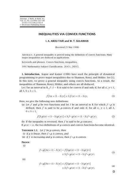
<strong>INEQUALITIES</strong> <strong>VIA</strong> <strong>CONVEX</strong> <strong>FUNCTIONS</strong><br />
I. A. ABOU-TAIR and W. T. SULAIMAN<br />
(Received 25 May 1998)<br />
Abstract. A general inequality is proved using the definition of convex functions. Many<br />
major inequalities are deduced as applications.<br />
Keywords and phrases. Convex functions, inequalities.<br />
1991 Mathematics Subject Classification. 26A51, 26D15.<br />
1. Introduction. Kapur and Kumer (1986) have used the principle of dynamical<br />
programming to prove major inequalities due to Shannon, Renyi, and Hölder. See [1].<br />
In this note, we prove a general inequality using convex functions. As a result, the<br />
inequalities of Shannon, Renyi, Hölder, and others are all deduced.<br />
Let I be an interval in R, f : I → R is said to be convex if and only if, for all x, y ∈ I,<br />
all λ, 0≤ λ ≤ 1,<br />
f [ λx +(1−λ)y ] ≤ λf (x)+(1−λ)y. (1)<br />
Here, we give the following new definitions:<br />
(a) Let f and g be two functions and let I be an interval in R for which f ◦ g is<br />
defined, then f is said to be g-convex if and only if, for all x, y ∈ I, all λ,<br />
0 ≤ λ ≤ 1,<br />
f [ λg(x)+(1−λ)g(y) ] ≤ λf ◦g(x)+(1−λ)f ◦g(y). (2)<br />
(b) If the inequality is reversed, then f is said to be g-concave.<br />
If g(x) = x, the two definitions of g-convex and convex functions become identical.<br />
Theorem 1.1. Let f be g-convex, then<br />
(i) if g is linear, then f ◦g is convex, and<br />
(ii) if f is increasing and g is convex, then f ◦g is convex.<br />
Proof.<br />
(i)<br />
(ii)<br />
f ◦g [ λx +(1−λ)y ] = f [ λg(x)+(1−λ)g(y) ]<br />
≤ λf ◦g(x)+(1−λ)f ◦g(y).<br />
f ◦g [ λx +(1−λ)y ] ≤ f [ λg(x)+(1−λ)g(y) ]<br />
≤ λf ◦g(x)+(1−λ)f ◦g(y).<br />
(3)<br />
(4)
544 I. A. ABOU-TAIR AND W. T. SULAIMAN<br />
Lemma 1.1. Let f be g-convex and let ∑ n<br />
i=1 t i = T n = 1, t i ≥ 0, i = 1,2,...,n, then<br />
(<br />
∑ n<br />
f t i g ( ) ) n∑<br />
x i ≤ t i f ◦g ( )<br />
x i . (5)<br />
Proof.<br />
(<br />
∑ n<br />
f<br />
i=1<br />
i=1<br />
t i g ( ) ) n−1<br />
∑<br />
x i =f<br />
(T n−1<br />
≤T n−1 f<br />
=T n−2 f<br />
i=1<br />
i=1<br />
t i<br />
g ( )<br />
x i +tn g ( ) )<br />
x n<br />
T n−1<br />
( n−1 ∑ t i<br />
g ( ) )<br />
x i +t n f ◦g ( )<br />
x n<br />
T<br />
i=1 n−1<br />
(<br />
n−2<br />
Tn−2 ∑<br />
T n−1<br />
i=1<br />
( n−2 ∑ t i<br />
i=1<br />
t i<br />
g ( ) t n−1<br />
x i + g ( ) )<br />
x n−1 +t n f ◦g ( )<br />
x n<br />
T n−2 T n−1<br />
(6)<br />
≤T n−2 f<br />
g ( ) )<br />
x i +t n−1 f ◦g ( )<br />
x n−1 +tn f ◦g ( )<br />
x n<br />
T n−2 .<br />
n∑<br />
≤ t i f ◦g ( )<br />
x i .<br />
i=1<br />
Lemma 1.2. For any function g, the exponential function f(x)= e x is g-convex.<br />
Proof.<br />
Define<br />
F(x)= λe g(x) +(1−λ)e g(y) −e λg(x)+(1−λ)g(y) . (7)<br />
Let<br />
G(t) = (1−λ)+λt −t λ , t >0. (8)<br />
It follows that<br />
G ′ (t) = λ ( 1−t λ−1) , G ′′ (t) = λ(1−λ)t λ−2 . (9)<br />
Thus, G ′ (t) = 0 when t = 1 and G ′′ (1) = λ(1 − λ) > 0. Hence, G has its minimum<br />
value 0 at t = 1 and this implies G(t) ≥ 0, t>0. The result follows by putting F(x)=<br />
e g(y) G(e g(x)−g(y) ).<br />
Corollary 1.3. The function f(x) = ln(x) is concave for if h(x) = e x , then, by<br />
Lemma 1.2, h is f -convex. Hence,<br />
It follows that<br />
e λ(lnx)+(1−λ)lny ≤ λe lnx +(1−λ)e lny = λx +(1−λy). (10)<br />
λlnx +(1−λ)lny ≤ ln [ λx +(1−λ)y ] . (11)<br />
2. Main inequality<br />
Theorem 2.1.<br />
Proof.<br />
n∑<br />
m∏<br />
j=1 i=1<br />
(<br />
pij<br />
) qi<br />
/ ∑mi=1<br />
q i<br />
≤<br />
∑ m<br />
i=1<br />
∑ n<br />
j=1 p ij q i<br />
∑ m<br />
i=1 q i<br />
. (12)<br />
If f(x)= e x and g(x) = lnx, then f is g-convex. By Lemma 1.2, we have
<strong>INEQUALITIES</strong> <strong>VIA</strong> <strong>CONVEX</strong> <strong>FUNCTIONS</strong> 545<br />
m∏<br />
/<br />
( ) ∑mi=1 (<br />
/ ∑mi=1 ∏mi=1<br />
)<br />
qi q i pij = e ln (p ij ) q i q i<br />
Therefore,<br />
i=1<br />
j=1 i=1<br />
/<br />
∑ ∑mi=1<br />
mi=1<br />
ln(p<br />
= e<br />
ij ) q i q ∑ i mi=1<br />
/ ∑mi=1<br />
(q<br />
= e i q i )lnp ij<br />
( ∑ m∑<br />
m<br />
qi<br />
≤ ∑ m<br />
)e lnp ij i=1 q i p ij<br />
= ∑ m .<br />
i=1 q i i=1 q i<br />
i=1<br />
(13)<br />
n∑ m∏<br />
/<br />
( ) ∑mi=1<br />
∑ n ∑ m ∑ m ∑ n<br />
qi q i j=1 i=1 p ij q i i=1 j=1 p ij q i<br />
pij ≤ ∑ m = ∑ m . (14)<br />
i=1 q i i=1 q i<br />
3. Applications<br />
Theorem 3.1 (Shannon’s inequality). Given ∑ m<br />
i=1 a i = a, ∑ m<br />
m∑<br />
Proof.<br />
we have<br />
That is<br />
It follows that<br />
Hence, we get<br />
( ) a<br />
aln ≤<br />
b<br />
i=1<br />
Applying Theorem 2.1 by putting<br />
p ij = b i<br />
a i<br />
, j = 1, q i = a i ,<br />
m∏<br />
i=1<br />
i=1 b i = b, then<br />
( )<br />
ai<br />
a i ln , a i ,b i ≥ 0. (15)<br />
b i<br />
m∑<br />
a i = a,<br />
i=1<br />
m∑<br />
b i = b, (16)<br />
/<br />
( ) ∑mi=1<br />
ai a bi<br />
i<br />
∑ m<br />
i=1 b<br />
≤ ∑ i<br />
m . (17)<br />
a i i=1 a i<br />
m∏<br />
i=1<br />
i=1<br />
(<br />
bi<br />
a i<br />
) ai /a<br />
≤ b a . (18)<br />
a<br />
m<br />
b ≤ ∏ ( ) ai /a ai<br />
. (19)<br />
b i<br />
i=1<br />
( ) a<br />
aln ≤<br />
b<br />
m∑<br />
i=1<br />
( )<br />
ai<br />
a i ln . (20)<br />
b i<br />
Theorem 3.2 (Renyi’s inequality). Given ∑ m<br />
i=1 a i = a, ∑ m<br />
i=1 b i = b, then, for α>0,<br />
α ̸=1,<br />
1 (<br />
a α b 1−α −a ) m∑ 1 ( )<br />
≤ a<br />
α<br />
i<br />
α−1<br />
α−1<br />
b1−α i<br />
−a i , ai ,b i ≥ 0. (21)<br />
i=1<br />
Proof. Applying Theorem 2.1 with i = 2, p 1j = c j , p 2j = d j , q 1 = λ, q 2 = 1 − λ,<br />
0
546 I. A. ABOU-TAIR AND W. T. SULAIMAN<br />
/∑ m<br />
/∑ m<br />
On putting c j = (a j j=1 a j ) and d j = (b j j=1 b j ), inequality (22) implies<br />
( m∑<br />
m<br />
)<br />
∑ λ ( m<br />
)<br />
∑ 1−λ<br />
a λ j b1−λ j<br />
≤ a j b j , (23)<br />
and this gives<br />
j=1<br />
j=1<br />
a λ b 1−λ<br />
λ−1 ≤ 1<br />
λ−1<br />
m∑<br />
j=1<br />
j=1<br />
a λ j b1−λ j<br />
. (24)<br />
Thus, for the case 0
Advances in Difference Equations<br />
Special Issue on<br />
Boundary Value Problems on Time Scales<br />
Call for Papers<br />
The study of dynamic equations on a time scale goes back<br />
to its founder Stefan Hilger (1988), and is a new area of<br />
still fairly theoretical exploration in mathematics. Motivating<br />
the subject is the notion that dynamic equations on time<br />
scales can build bridges between continuous and discrete<br />
mathematics; moreover, it often revels the reasons for the<br />
discrepancies between two theories.<br />
In recent years, the study of dynamic equations has led<br />
to several important applications, for example, in the study<br />
of insect population models, neural network, heat transfer,<br />
and epidemic models. This special issue will contain new<br />
researches and survey articles on Boundary Value Problems<br />
on Time Scales. In particular, it will focus on the following<br />
topics:<br />
• Existence, uniqueness, and multiplicity of solutions<br />
• Comparison principles<br />
• Variational methods<br />
• Mathematical models<br />
• Biological and medical applications<br />
• Numerical and simulation applications<br />
Lead Guest Editor<br />
Alberto Cabada, Departamento de Análise Matemática,<br />
Universidade de Santiago de Compostela, 15782 Santiago de<br />
Compostela, Spain; alberto.cabada@usc.es<br />
Guest Editor<br />
Victoria Otero-Espinar, Departamento de Análise<br />
Matemática, Universidade de Santiago de Compostela,<br />
15782 Santiago de Compostela, Spain;<br />
mvictoria.otero@usc.es<br />
Before submission authors should carefully read over the<br />
journal’s Author Guidelines, which are located at http://www<br />
.hindawi.com/journals/ade/guidelines.html. Authors should<br />
follow the Advances in Difference Equations manuscript<br />
format described at the journal site http://www.hindawi<br />
.com/journals/ade/. Articles published in this Special Issue<br />
shall be subject to a reduced Article Processing Charge of<br />
C200 per article. Prospective authors should submit an electronic<br />
copy of their complete manuscript through the journal<br />
Manuscript Tracking System at http://mts.hindawi.com/<br />
according to the following timetable:<br />
Manuscript Due April 1, 2009<br />
First Round of Reviews July 1, 2009<br />
Publication Date October 1, 2009<br />
Hindawi Publishing Corporation<br />
http://www.hindawi.com