Inter-universal Teichmuller Theory I: Construction of Hodge Theaters

24.04.2014 Views
112 SHINICHI MOCHIZUKI — which [since Π p0 is commensurably terminal in π 1 ( † D ⊛ ) — cf., e.g., [AbsAnab], Theorem 1.1.1, (i)] we consider up to the action by the “inner automorphisms of the pair” arising from conjugation by Π p0 . In the language of [AbsTopIII], §3, this pair is an “MLF-Galois TM-pair of strictly Belyi type” [cf. [AbsTopIII], Definition 3.1, (ii)]. (vi) Before proceeding, we observe that the discussion of (iv), (v) concerning † F ⊛ , † D ⊛ may also be carried out for † F ⊚ , † D ⊚ . We leave the routine details to the reader. (vii) Next, let us consider the index set J of the capsule of D-prime-strips † D J . def ∼ For j ∈ J, writeV j = {v j } v∈V . Thus, we have a natural bijection V j → V, i.e., given by sending v j ↦→ v. These bijections determine a “diagonal subset” V 〈J〉 ⊆ V J def = ∏ j∈J V j — which also admits a natural bijection V 〈J〉 ∼ → V. Thus,weobtainnatural bijections V 〈J〉 ∼ → Vj ∼ → Prime( † F ⊚ mod ) ∼ → V mod for j ∈ J. Write † F ⊚ 〈J〉 † F ⊚ j def = { † F ⊚ mod , V 〈J〉 def = { † F ⊚ mod , V j ∼ → Prime( † F ⊚ mod )} ∼ → Prime( † F ⊚ mod )} for j ∈ J. That is to say, we think of † F ⊚ j as a copy of † F ⊚ mod “situated on” the constituent labeled j of the capsule † D J ; we think of † F ⊚ 〈J〉 as a copy of † F ⊚ mod “situated in a diagonal fashion on” all the constituents of the capsule † D J . Thus, we have a natural embedding of categories † F ⊚ 〈J〉 ↩→ † F ⊚ J def = ∏ j∈J † F ⊚ j — where, by abuse of notation, we write † F ⊚ 〈J〉 for the underlying category of [i.e., the first member of the pair] † F ⊚ 〈J〉 . Here, we observe that the category † F ⊚ J is not equipped with a Frobenioid structure. Write † F ⊚R j ; † F ⊚R 〈J〉 ; † F ⊚R J def = ∏ j∈J † F ⊚R j for the respective realifications [or product of the underlying categories of the realifications] of the corresponding Frobenioids whose notation does not contain a superscript “R”. [Here, we recall that the theory of realifications of Frobenioids is discussed in [FrdI], Proposition 5.3.] Remark 5.1.1. Thus, † F ⊚ 〈J〉 may be thought of as the Frobenioid associated to divisors on V J [i.e., finite formal sums of elements of this set with coefficients in Z or

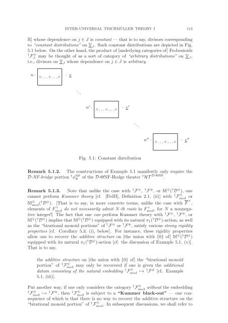
INTER-UNIVERSAL TEICHMÜLLER THEORY I 113 R] whose dependence on j ∈ J is constant — that is to say, divisors corresponding to “constant distributions” on V J . Such constant distributions are depicted in Fig. 5.1 below. On the other hand, the product of [underlying categories of] Frobenioids † F ⊚ J may be thought of as a sort of category of “arbitrary distributions” on V J, i.e., divisors on V J whose dependence on j ∈ J is arbitrary. n · ◦ ...◦ ...◦ · v . .. n ′ · ◦ ...◦ ...◦ · v ′ . .. n ′′ · ◦ ...◦ ...◦ · v ′′ Fig. 5.1: Constant distribution Remark 5.1.2. The constructions of Example 5.1 manifestly only require the D-NF-bridge portion † φ NF of the D-ΘNF-Hodge theater † HT D-ΘNF . Remark 5.1.3. Note that unlike the case with † F ⊚ , † F ⊛ ,orM ⊚ ( † D ⊚ ), one cannot perform Kummer theory [cf. [FrdII], Definition 2.1, (ii)] with † F ⊚ mod or M ⊚ mod († D ⊚ ). [That is to say, in more concrete terms, unlike the case with F × , elements of F × mod do not necessarily admit N-th roots in F × mod ,forN a nonnegative integer!] The fact that one can perform Kummer theory with † F ⊚ , † F ⊛ ,or M ⊚ ( † D ⊚ ) implies that M ⊚ ( † D ⊚ ) equipped with its natural π 1 ( † D ⊚ )-action, as well as the “birational monoid portions” of † F ⊚ or † F ⊛ , satisfy various strong rigidity properties [cf. Corollary 5.3, (i), below]. For instance, these rigidity properties allow one to recover the additive structure on [the union with {0} of] M ⊚ ( † D ⊚ ) equipped with its natural π 1 ( † D ⊚ )-action [cf. the discussion of Example 5.1, (v)]. That is to say, the additive structure on [the union with {0} of] the “birational monoid portion” of † F ⊚ mod may only be recovered if one is given the additional datum consisting of the natural embedding † F ⊚ mod ↩→ † F ⊛ [cf. Example 5.1, (iii)]. Put another way, if one only considers the category † F ⊚ mod without the embedding † F ⊚ mod ↩→ † F ⊛ ,then † F ⊚ mod is subject to a “Kummer black-out” — one consequence of which is that there is no way to recover the additive structure on the “birational monoid portion” of † F ⊚ mod . In subsequent discussions, we shall refer to

Page 1 and 2: INTER-UNIVERSAL TEICHMÜLLER THEORY







Page 15 and 16: associated to † F ⊩ mod and ‡

































Page 81 and 82: completely determined by † D. INT








Page 97 and 98: conjugation by which maps φ NF IN







Page 111: INTER-UNIVERSAL TEICHMÜLLER THEORY








Page 129 and 130: (v) Write INTER-UNIVERSAL TEICHMÜL














Page 157: INTER-UNIVERSAL TEICHMÜLLER THEORY

remark

definition

proposition

associated

various

corollary

isomorphism

follows

theorem

mochizuki

teichmuller

hodge

theaters

www.kurims.kyoto-u.ac.jp

Inter-universal Teichmuller Theory I: Construction of Hodge Theaters

Inter-universal Teichmuller Theory I: Construction of Hodge Theaters ... View more Inter-universal Teichmuller Theory I: Construction of Hodge Theaters

Delete template?

Save as template ?

Inter-universal Teichmuller Theory I: Construction of Hodge Theaters Inter-universal Teichmuller Theory I: Construction of Hodge Theaters