Laplace Transforms

Laplace Transforms
Gilles Cazelais
May 2006

Contents
1 Problems 1
1.1 Laplace Transforms . . . . . . . . . . . . . . . . . . . . . . . . . . 1
1.2 Inverse Laplace Transforms . . . . . . . . . . . . . . . . . . . . . 2
1.3 Initial Value Problems . . . . . . . . . . . . . . . . . . . . . . . . 3
1.4 Step Functions and Impulses . . . . . . . . . . . . . . . . . . . . 4
1.5 Convolution . . . . . . . . . . . . . . . . . . . . . . . . . . . . . . 5
2 Solutions 7
2.1 Laplace Transforms . . . . . . . . . . . . . . . . . . . . . . . . . . 7
2.2 Inverse Laplace Transforms . . . . . . . . . . . . . . . . . . . . . 10
2.3 Initial Value Problems . . . . . . . . . . . . . . . . . . . . . . . . 16
2.4 Step Functions and Impulses . . . . . . . . . . . . . . . . . . . . 25
2.5 Convolution . . . . . . . . . . . . . . . . . . . . . . . . . . . . . . 33
A Formulas and Properties 39
A.1 Table of Laplace Transforms . . . . . . . . . . . . . . . . . . . . . 39
A.2 Properties of Laplace Transforms . . . . . . . . . . . . . . . . . . 40
A.3 Trigonometric Identities . . . . . . . . . . . . . . . . . . . . . . . 41
B Partial Fractions 43
B.1 Partial Fractions . . . . . . . . . . . . . . . . . . . . . . . . . . . 43
B.2 Cover-up Method . . . . . . . . . . . . . . . . . . . . . . . . . . . 44
Bibliography 47
i

ii
CONTENTS

Chapter 1
Problems
1.1 Laplace Transforms
1. Find the Laplace transform of the following functions.
(d) f(t) = e −2t (4 cos 5t + 3 sin 5t)
(a) f(t) = 4t 2 − 2t + 3
(b) f(t) = 3 sin 5t − 2 cos 3t
(e) f(t) = t 3 e 2t + 2te −t
(c) f(t) = 3e 2t + 5e −3t (f) f(t) = (1 + e 3t ) 2
2. Use an appropriate trigonometric identity to find the following Laplace transforms.
See page 41 for a list of trigonometric identities.
(a) L { cos 2 t }
(b) L {sin 2t cos 2t}
(c) L {sin 3t cos 4t}
(d) L {sin(ωt + φ)}
(e) L {cos(ωt + φ)}
(f) L { e −2t sin(3t + π 6 )}
3. The hyperbolic sine and hyperbolic cosine are defined by
sinh t = et − e −t
and cosh t = et + e −t
.
2
2
Evaluate both L {sinh ωt} and L {cosh ωt}.
4. Find both L {cos ωt} and L {sin ωt} by starting from Euler’s formula
and
e jθ = cos θ + j sin θ
L { e at} = 1
s − a .
1

2 CHAPTER 1. PROBLEMS
5. Use the frequency differentiation property (see page 40) to derive the following
formulas.
(a) L {t sin ωt} =
2ωs (b) L {t cos ωt} = s2 − ω 2
(s 2 + ω 2 ) 2
(s 2 + ω 2 ) 2
6. Use the frequency shift property (see page 40) to find the following.
(a) L { t e 2t sin 3t } (b) L { t e −3t cos 2t }
1.2 Inverse Laplace Transforms
In problems 1 − 8, find the inverse Laplace transforms of the given functions.
1. F (s) = 1 5. F (s) =
s 4
2. F (s) = s + 5
s 2 + 4
3. F (s) = 3s + 1
7. F (s) =
s 2 + 5
1
4. F (s) =
(s − 3) 5 8. F (s) =
s − 2
s 2 + 2s + 5
6. F (s) = s + 5
(s 2 + 9) 2
1
s 2 − 4s + 7
5s + 2
(s 2 + 6s + 13) 2
In problems 9 − 16, use the method of partial fractions to find the given inverse
Laplace transforms. See page 43 for a refresher on partial fractions.
{ } s + 3
9. L −1 s 2 + 4s − 5
{
}
10. L −1 s + 1
(2s − 1)(s + 2
{ s
11. L −1 2 }
+ s + 5
s 4 − s 2
{
}
12. L −1 1
(s + 1)(s 2 + 4)
{ s
13. L −1 2 }
+ 3s + 4
(s − 2) 3
{ s
14. L −1 2 }
+ s + 4
s 3 + 9s
{ } 3s + 2
15. L −1 s 3 (s 2 + 1)
{
}
16. L −1 2s + 1
(s + 3)(s 2 + 4s + 13)

1.3. INITIAL VALUE PROBLEMS 3
1.3 Initial Value Problems
Use Laplace transforms to solve the following initial-value problems.
1. y ′ + 4y = e t , y(0) = 2
2. y ′ − y = sin t, y(0) = 1
3. y ′′ + 3y ′ + 2y = t + 1, y(0) = 1, y ′ (0) = 0
4. y ′′ + 4y ′ + 13y = 0, y(0) = 1, y ′ (0) = 2
5. y ′′ + 4y = 4t + 8, y(0) = 4, y ′ (0) = −1
6. y ′′ + y ′ − 2y = 5e 3t , y(0) = 1, y ′ (0) = −4
7. y ′′ + y ′ − 2y = e t , y(0) = 2, y ′ (0) = 3
8. y ′′ − 2y ′ + y = e t , y(0) = 3, y ′ (0) = 4
9. y ′′ + 2y ′ + 2y = cos 2t, y(0) = 0, y ′ (0) = 1
10. y ′′ + 4y = sin 3t, y(0) = 2, y ′ (0) = 1
11. y ′′ + ω 2 y = cos ωt, y(0) = 0, y ′ (0) = 0
12. y ′′ + 2y ′ + 5y = 3e −t cos 2t, y(0) = 1, y ′ (0) = 2
13. The differential equation for a mass-spring system is
mx ′′ (t) + βx ′ (t) + kx(t) = F e (t).
Consider a mass-spring system with a mass m = 1 kg that is attached to a
spring with constant k = 5 N/m. The medium offers a damping force six
times the instantaneous velocity, i.e., β = 6 N· s/m.
(a) Determine the position of the mass x(t) if it is released with initial
conditions: x(0) = 3 m, x ′ (0) = 1 m/s. There is no external force.
(b) Determine the position of the mass x(t) if it released with the initial
conditions: x(0) = 0, x ′ (0) = 0 and the system is driven by an external
force F e (t) = 30 sin 2t in newtons with time t measured in seconds.
14. The differential equation for the current i(t) in an LR circuit is
L di + Ri = V (t).
dt
Find the current in an LR circuit if the initial current is i(0) = 0 A given that
L = 2 H, R = 4 Ω, and V (t) = 5e −t volts with time t measured in seconds..
15. The differential equations for the charge q(t) in an LRC circuit is
Lq ′′ (t) + Rq ′ (t) + q(t)
C
= V (t).
Find the charge and current in an LRC circuit with L = 1 H, R = 2 Ω,
C = 0.25 F and V = 50 cos t volts if q(0) = 0 C and i(0) = 0 A.

4 CHAPTER 1. PROBLEMS
1.4 Step Functions and Impulses
1. Find the Laplace transforms of the following functions.
⎧
⎧
⎪⎨ t, 0 ≤ t < 1
⎪⎨ 1, 0 ≤ t < 1
(c) f(t) = 1, 1 ≤ t < 2
(a) f(t) = 3, 1 ≤ t < 2
⎪⎩
⎪⎩
0, t ≥ 2
−2, t ≥ 2
{
{
sin t, 0 ≤ t < π
0, 0 ≤ t < 3
(b) f(t) =
(d) f(t) =
0, t ≥ π
t 2 , t ≥ 3
2. Find the following inverse Laplace transforms.
{ } e
(a) L −1 −2s
s + 3
{ } e
(b) L −1 −2πs
s 2 + 4
(c) L −1 {
(d) L −1 {
e −s
(s − 1)(s + 2)
e
−πs
s(s 2 + 1)
In problems 3 − 9, use Laplace transforms solve the initial-value problem.
to
{
3. y ′ + 2y = f(t), y(0) = 3, where f(t) =
1, 0 ≤ t ≤ 1
0, t ≥ 1
{
4. y ′′ + y = f(t), y(0) = 1, y ′ (0) = 0, where f(t) =
0, 0 ≤ t ≤ π
sin t, t ≥ π
{
5. y ′′ + y ′ − 2y = f(t), y(0) = 0, y ′ (0) = 0, where f(t) =
1, 0 ≤ t ≤ 3
−1, t ≥ 3
⎧
⎪⎨ 1, 0 ≤ t < π,
6. y ′′ + 4y = f(t), y(0) = 0, y ′ (0) = 2, where f(t) = 2, π ≤ t < 2π,
⎪⎩
0, t ≥ 2π
7. y ′ + 3y = δ(t − 1), y(0) = 2
8. y ′′ + 4y ′ + 13y = δ(t − π), y(0) = 2, y ′ (0) = 1
9. y ′′ + y = δ(t − π 2 ) + 2δ(t − π), y(0) = 3, y′ (0) = −1
10. Find the Laplace transform of the periodic function f(t) with period T = 2a
defined over one period by
{
1, 0 ≤ t < a
f(t) =
0, a ≤ t < 2a.
}
}

1.5. CONVOLUTION 5
11. The differential equation for the current i(t) in an LR circuit is
L di + Ri = V (t).
dt
Consider an LR circuit with L = 1 H, R = 4 Ω and a voltage source (in volts)
{
2, 0 ≤ t < 1
V (t) =
0, t ≥ 1.
(a) Find the current i(t) if i(0) = 0.
(b) Compute the current at t = 1.5 seconds, i.e., compute i(1.5).
(c) Evaluate lim
t→∞
i(t).
(d) Sketch the graph of the current as a function of time.
12. Consider the following function with a > 0 and ɛ > 0.
⎧
0, 0 ≤ t < a
⎪⎨
1
δ ε (t − a) =
⎪⎩
ε , a ≤ t < a + ε
0, t ≥ a + ε
(a) Find L {δ ε (t − a)}.
(b) Show that: lim
ε→0
L {δ ε (t − a)} = e −as .
1.5 Convolution
1. Find the following Laplace transforms.
(a) L { 1 ∗ t 4}
{∫ t
}
(b) L cos θ dθ
0
(c) L {e t ∗ sin t}
{∫ t
}
(d) L cos θ sin(t − θ) dθ
0
2. Find the following inverse Laplace transforms by using convolution. Do not
use partial fractions.
{ }
{ }
(a) L −1 1
(c) L −1 1
s(s 2 + 1))
s(s − 1)
{
}
{ }
(b) L −1 1
(d) L −1 1
(s + 1)(s − 3)
s 2 (s 2 + 1)

6 CHAPTER 1. PROBLEMS
3. Use convolution to derive the following formula.
{ }
L −1 1 sin ωt − ωt cos ωt
(s 2 + ω 2 ) 2 =
2ω 3
4. Solve for f(t) in the following equation.
f(t) = t + e 2t +
∫ t
0
e −θ f(t − θ) dθ
5. Solve for f(t) in the following equation. Be sure to find all solutions.
∫ t
0
f(θ)f(t − θ) dθ = t 3
6. Solve for y(t) in the following initial-value problem.
y ′ (t) +
∫ t
0
e −2θ y(t − θ) dθ = 1, y(0) = 0

Chapter 2
Solutions
2.1 Laplace Transforms
1. We use the table of Laplace transforms (see page 39) to answer this question.
(a) L {f(t)} = 4 L { t 2} − 2 L {t} + 3 L {1} = 8 s 3 − 2 s 2 + 3 s
(b) L {f(t)} = 3 L {sin 5t} − 2 L {cos 3t} = 15
s 2 + 25 −
2s
s 2 + 9
(c) L {f(t)} = 3 L { e 2t} + 5 L { e −3t} = 3
s − 2 + 5
s + 3
(d) L {f(t)} = 4 L { e −2t cos 5t } +3 L { e −2t sin 5t } 4(s + 2)
=
(s + 2) 2 + 25 + 15
(s + 2) 2 + 25
(e) L {f(t)} = L { t 3 e 2t} + 2 L {te −t 6
} =
(s − 2) 4 + 2
(s + 1) 2
(f) Since f(t) = (1 + e 3t ) 2 = 1 + 2e 3t + e 6t , we have
2. (a) Since cos 2 t =
L {f(t)} = L {1} + 2L { e 3t} + L { e 6t} = 1 s + 2
s − 3 + 1
s − 6 .
1 + cos 2t
, we have
2
L { cos 2 t } = 1 (L {1} + L {cos 2t})
2
= 1 ( 1
2 s + s )
s 2 .
+ 4
(b) Starting from the identity sin 2θ = 2 sin θ cos θ, if we let θ = 2t we get
sin 4t = 2 sin 2t cos 2t =⇒ sin 2t cos 2t = 1 sin 4t
2
7

8 CHAPTER 2. SOLUTIONS
and
L {sin 2t cos 2t} = 1 2 L {sin 4t} = 1 2
( ) 4 2
s 2 =
+ 16 s 2 + 16 .
(c) From the identity sin α cos β = 1 2
(sin(α + β) + sin(α − β)), we deduce
and
sin 3t cos 4t = 1 (sin(3t + 4t) + sin(3t − 4t))
2
L {sin 3t cos 4t} = 1 2
= 1 (sin 7t + sin(−t))
2
= 1 (sin 7t − sin t)
2
( 7
s 2 + 49 − 1 )
s 2 .
+ 1
(d) From the identity sin(α + β) = sin α cos β + cos α sin β, we deduce
and
sin(ωt + φ) = sin ωt cos φ + cos ωt sin φ
L {sin(ωt + φ)} = cos φ L {sin ωt} + sin φ L {cos ωt}
( ) ( )
ω
s
= cos φ
s 2 + ω 2 + sin φ
s 2 + ω 2 .
(e) From the identity cos(α + β) = cos α cos β − sin α sin β, we deduce
and
cos(ωt + φ) = cos ωt cos φ − sin ωt sin φ
L {cos(ωt + φ)} = cos φ L {cos ωt} − sin φ L {sin ωt}
( ) ( )
s
ω
= cos φ
s 2 + ω 2 − sin φ
s 2 + ω 2 .
(f) Using the identity sin(α + β) = sin α cos β + cos α sin β, we deduce
e −2t sin(3t + π 6 ) = e−2t (sin 3t cos π 6 + cos 3t sin π 6 )
and
L { √ ( 3
e −2t sin(3t + π 6 )} =
2
= e −2t ( √ 3
2 sin 3t + 1 2
cos 3t)
= √ 3
2 e−2t sin 3t + 1 2 e−2t cos 3t
3
(s + 2) 2 + 9
)
+ 1 (
2
s + 2
(s + 2) 2 + 9
)
.

2.1. LAPLACE TRANSFORMS 9
3. Using L {e at } = 1 , we deduce
s − a
and
4. From Euler’s formula, we get
From L {e at } = 1 , we deduce
s − a
L {sinh ωt} = 1 ( {
L e
ωt } − L { e −ωt} )
2
= 1 ( 1
2 s − ω − 1 )
s + ω
= 1 ( )
s + ω − (s − ω)
2 s 2 − ω 2
ω
=
s 2 − ω 2
L {cosh ωt} = 1 ( {
L e
ωt } + L { e −ωt} )
2
= 1 ( 1
2 s − ω + 1 )
s + ω
= 1 ( )
s + ω + s − ω
2 s 2 − ω 2
s
=
s 2 − ω 2 .
L { e jωt} =
L { e jωt} = L {cos ωt} + jL {sin ωt} . (2.1)
1
s − jω = 1
s − jω
( ) s + jω
= s + jω
s + jω s 2 + ω 2 . (2.2)
Since the real and imaginary parts in equations (2.1) and (2.2) are equal, we
conclude that
L {cos ωt} =
s
ω
s 2 + ω 2 and L {sin ωt} =
s 2 + ω 2 .
5. We will use the property L {tf(t)} = −F ′ (s).
(a) If f(t) = sin ωt, we have F (s) =
ω
s 2 + ω 2 . Therefore
L {t sin ωt} = −F ′ (s) = − d ds
2ωs
=
(s 2 + ω 2 ) 2 .
( ω
s 2 + ω 2 )

10 CHAPTER 2. SOLUTIONS
s
(b) If f(t) = cos ωt, we have F (s) =
s 2 + ω 2 . Therefore
L {t cos ωt} = −F ′ (s) = − d ( )
s
ds s 2 + ω 2
= s2 − ω 2
(s 2 + ω 2 ) 2 .
6. We use the frequency shift property L {e at f(t)} = F (s − a).
(a) Since L {t sin 3t} =
L { te 2t sin 3t } =
6s
(s 2 , we conclude that
+ 9)
2
6(s − 2)
((s − 2) 2 + 9) 2 = 6(s − 2)
(s 2 − 4s + 13) 2 .
(b) Since L {t cos 2t} = s2 − 4
(s 2 , we conclude that
+ 4)
2
L { te −3t cos 2t } = (s + 3)2 − 4
((s + 3) 2 + 4) 2 = s2 + 6s + 5
(s 2 + 6s + 13) 2 .
2.2 Inverse Laplace Transforms
1. L −1 { 1
s 4 }
= 1 3! L −1 { 3!
s 4 }
= t3 6
{ } { }
s + 5
s
2. L −1 s 2 = L −1
+ 4
s 2 + 5 { } 2
+ 4 2 L −1 s 2 = cos 2t + 5 sin 2t
+ 4
2
{ } { }
{
3s + 1
s
3. L −1 s 2 = 3L −1
+ 5
s 2 + 1
√ }
5
√ L −1
+ 5 5 s 2 + 5
{ }
4. L −1 1
(s − 3) 5
5. By completing the square, we get
{ } 3s + 1
L −1 s 2 = 3 cos √ 5t + √ 1 sin √ 5t
+ 5
5
= 1 { } 4!
4! L −1 (s − 3) 5 = t4 e 3t
24
s 2 + 2s + 5 = (s + 1) 2 + 4.
Observe that
s − 2 (s + 1) − 3
s 2 =
+ 2s + 5 (s + 1) 2 + 4 .

2.2. INVERSE LAPLACE TRANSFORMS 11
Therefore,
L −1 { s − 2
s 2 + 2s + 5
{ } s + 5
6. L −1 (s 2 + 9) 2
}
= L −1 {
s + 1
(s + 1) 2 + 4
= e −t cos 2t − 3 2 e−t sin 2t.
}
− 3 2 L −1 {
= 1 { } { }
6 L −1 6s
(s 2 + 9) 2 + 5L −1 1
(s 2 + 9) 2
{ } s + 5
L −1 (s 2 + 9) 2 = 1 ( sin 3t − 3t cos 3t
6 t sin 3t + 5 2(3 3 )
= 1 6 t sin 3t + 5 54 sin 3t − 5 t cos 3t.
18
}
2
(s + 1) 2 + 4
)
7. By completing the square, we get
s 2 − 4s + 7 = (s − 2) 2 + 3.
Therefore,
{
}
L −1 1
s 2 − 4s + 7
{
= √ 1
√ }
3
L −1
3 (s − 2) 2 + 3
= 1 √
3
e 2t sin √ 3t.
8. First we complete the square to get
Observe that
s 2 + 6s + 13 = (s + 3) 2 + 4.
5s + 2 5(s + 3) − 13
(s 2 =
+ 6s + 13)
2
((s + 3) 2 + 4) 2 .
We now use the frequency shift theorem L {e at f(t)} = F (s − a) to conclude
that
{ }
{ }
5(s + 3) − 13
5s − 13
L −1 ((s + 3) 2 + 4) 2 = e −3t L −1 (s 2 + 4) 2 .
{ } 5s − 13
Now let’s focus on L −1 (s 2 + 4) 2 .
{ } 5s − 13
L −1 (s 2 + 4) 2
= 5 { } { }
4 L −1 4s
(s 2 + 4) 2 − 13L −1 1
(s 2 + 4) 2
= 5 ( )
sin 2t − 2t cos 2t
4 t sin 2t − 13 2(2) 3
= 5 13
t sin 2t −
4 16
13
sin 2t + t cos 2t
8

12 CHAPTER 2. SOLUTIONS
Therefore,
{
} (
L −1 5s + 2
5
(s 2 + 6s + 13) 2 = e −3t 4
t sin 2t −
13
16 sin 2t + 13 8 t cos 2t )
.
9. We can factor the denominator to obtain
s 2 + 4s − 5 = (s − 1)(s + 5).
The partial fractions decomposition is of the form
s + 3
(s − 1)(s + 5) = A
s − 1 + B
s + 5 .
Using the cover-up method we obtain A and B as follows.
s + 3
A =
✘(s ✘ − ✘
= 2 s + 3
and B =
1) (s + 5) ∣ 3
s=1
(s − 1) ✘(s ✘ + ✘
= 1
5) ∣ 3
s=−5
Then,
{
}
L −1 s + 3
(s − 1)(s + 5)
= 2 { } 1
3 L −1 + 1 { } 1
s − 1 3 L −1 s + 5
= 2 3 et + 1 3 e−5t .
10. The partial fractions decomposition is of the form
s + 1
(2s − 1)(s + 2) = A
2s − 1 + B
s + 2 .
Using the cover-up method we obtain A and B as follows.
s + 1
A =
✘(2s ✘ = 3 s + 1
and B =
−✘✘
1) (s + 2) ∣ 5
s=1/2
(2s − 1) ✘(s ✘ + ✘
= 1
2) ∣ 5
s=−2
Then,
{
}
L −1 s + 1
(2s − 1)(s + 2)
= 3 { } 1
5 L −1 2s − 1
= 3
5 · 2 L −1 { 1
s − 1/2
= 3 10 et/2 + 1 5 e−2t .
+ 1 { } 1
5 L −1 s + 2
}
+ 1 { 1
5 L −1 s + 2
}

2.2. INVERSE LAPLACE TRANSFORMS 13
11. We start by factoring the denominator to get s 4 − s 2 = s 2 (s − 1)(s + 1). The
partial fractions decomposition is of the form
s 2 + s + 5
s 2 (s − 1)(s + 1) = A s + B s 2 +
C
s − 1 +
By multiplying both sides by s 2 (s − 1)(s + 1) we get
D
s + 1 .
s 2 + s + 5 = As(s − 1)(s + 1) + B(s − 1)(s + 1) + Cs 2 (s + 1) + Ds 2 (s − 1).
To find the constants, let’s assign values to s as follows.
s = 0 =⇒ 5 = 0 − B + 0 + 0 =⇒ B = −5
s = 1 =⇒ 7 = 0 + 0 + 2C + 0 =⇒ C = 7/2
s = −1 =⇒ 5 = 0 + 0 + 0 − 2D =⇒ D = −5/2
s = 2 =⇒ 11 = 6A + 3B + 12C + 4D =⇒ A =
11 − 3B − −12C − 4D
6
= −1
Then,
{ s
L −1 2 } { } { }
+ s + 5
1 1
s 4 − s 2 = −L −1 − 5L −1
s
s 2 + 7 { } 1
2 L −1 − 5 { } 1
s − 1 2 L −1 s + 1
= −1 − 5t + 7 2 et − 5 2 e−t .
12. The partial fractions decomposition is of the form
1
(s + 1)(s 2 + 4) = A
s + 1 + Bs + c
s 2 + 4 .
We can use the cover-up method to find A, B, C as follows.
1
A =
✘✘ (s + ✘
= 1
1) (s 2 + 4) ∣ 5
s=−1
(Bs + C)| s=2j =
2Bj + C = 1
1 + 2j
= 1
1 + 2j
1
(s + 1) ✘✘ (s 2 + ✘ 4)
= 1 − 2j .
5
∣
( ) 1 − 2j
1 − 2j
∣
s=2j

14 CHAPTER 2. SOLUTIONS
Since the real and imaginary parts are equal on both sides, we get
B = − 1 5
and C = 1 5 .
Then,
{
}
L −1 1
(s + 1)(s 2 + 4)
= 1 { } 1
5 L −1 s + 1
= 1 5 e−t − 1 5
− 1 { s
5 L −1 s 2 + 4
1
cos 2t + sin 2t.
10
13. The partial fractions decomposition is of the form
s 2 + 3s + 4
(s − 2) 3 = A
s − 2 + B
(s − 2) 2 + C
(s − 2) 3 .
By multiplying both sides by (s − 3) 3 and expanding, we get
We conclude that
Then,
s 2 + 3s + 4 = A(s − 2) 2 + B(s − 2) + C
= A(s 2 − 4s + 4) + Bs − 2B + C
= As 2 + (B − 4A)s + (C − 2B + 4A).
A = 1, B − 4A = 3 =⇒ B = 7, C − 2B + 4A = 4 =⇒ C = 14.
{ s
L −1 2 } {
+ 3s + 4
1
(s − 2) 3 = L −1 s − 2
}
+ 7L −1 {
= e 2t + 7te 2t + 7t 2 e 2t .
}
+ 1 { } 2
5 · 2 L −1 s 2 + 4
}
1
(s − 2) 2 + 14 { } 2!
2! L −1 (s − 2) 3
14. We factor the denominator to get s 3 + 9s = s(s 2 + 9). The partial fractions
decomposition is of the form
s 2 + s + 4
s(s 2 + 9) = A s + Bs + C
s 2 + 9 .
By multiplying both sides by s(s 2 + 9) and expanding, we get
We conclude that
s 2 + s + 4 = A(s 2 + 9) + (Bs + C)s
= As 2 + 9A + Bs 2 + Cs
= (A + B)s 2 + Cs + 9A.
9A = 4 =⇒ A = 4/9, C = 1, A + B = 1 =⇒ B = 5/9.

2.2. INVERSE LAPLACE TRANSFORMS 15
Then,
L −1 { s 2 + s + 4
s 3 + 9s
}
= 4 { 1
9 L −1 s
= 4 9 + 5 9 cos 3t + 1 sin 3t.
3
}
+ 5 { } s
9 L −1 s 2 + 1 { } 3
+ 9 3 L −1 s 2 + 9
15. The partial fractions decomposition is of the form
3s + 2
s 3 (s 2 + 1) = A s + B s 2 + C s 3 + Ds + E
s 2 + 1 .
By multiplying both sides by s 3 (s 2 + 1) and expanding, we get
3s + 2 = As 2 (s 2 + 1) + Bs(s 2 + 1) + C(s 2 + 1) + (Ds + E)s 3
= As 4 + As 2 + Bs 3 + Bs + Cs 2 + C + Ds 4 + Es 3
0s 4 + 0s 3 + 0s 2 + 3s + 2 = (A + D)s 4 + (B + E)s 3 + (A + C)s 2 + Bs + C.
We conclude that
C = 2
B = 3
A + C = 0 =⇒ A = −2
B + E = 0 =⇒ E = −3
A + D = 0 =⇒ D = 2.
Then,
{ } 3s + 2
L −1 s 3 (s 2 = −2 + 3t + t 2 + 2 cos t − 3 sin t.
+ 1)
16. First we complete the square to get s 2 + 4s + 13 = (s + 2) 2 + 9. We can look
for a partial fractions decomposition in the form
2s + 1
(s + 3)(s 2 + 4s + 13) = A B(s + 2) + C
+
s + 3 (s + 2) 2 + 9 .
Method 1. Let’s multiply both sides by (s + 3)((s + 2) 2 + 9) to get
2s + 1 = A((s + 2) 2 + 9) + (B(s + 2) + C)(s + 3).
To find the constants A, B, and C, let’s assign values to s as follows.
s = −3 =⇒ −5 = 10A + 0 =⇒ A = −1/2
s = −2 =⇒ −3 = 9A + C =⇒ C = −3 − 9A = 3/2
s = −1 =⇒ −1 = 10A + 2B + 2C =⇒ B = (−3 − 10A − 2C)/2 = 1/2

16 CHAPTER 2. SOLUTIONS
Method 2. We can use the cover-up method to find A, B, and C.
2s + 1
A =
✘(s ✘ + ✘
= − 1
3) (s 2 + 4s + 13) ∣ 2 .
s=−3
Since s 2 + 4s + 13 = (s + 2) 2 + 9 = 0 if s = −2 + 3j, then
2s + 1
(B(s + 2) + C)| s=−2+3j =
✭ ∣
(s + 3) ✭✭✭✭✭
(s 2 + 4s + 13)
2(−2 + 3j) + 1
3Bj + C =
(−2 + 3j) + 3
−3 + 6j
=
1 + 3j
( ) ( )
−3 + 6j 1 − 3j
=
1 + 3j 1 − 3j
15j + 15
3Bj + C = .
10
∣
s=−2+3j
Since the real and imaginary parts are equal on both sides, we get
Then,
3B = 15
10 =⇒ B = 1 2
2s + 1
(s + 3)(s 2 + 4s + 13) = −1 2
( ) 1
+ 1 (
s + 3 2
and C = 15
10 = 3 2 .
s + 2
(s + 2) 2 + 9
)
+ 1 (
2
3
(s + 2) 2 + 9
)
and
{
}
L −1 2s + 1
(s + 3)(s 2 = − 1 + 4s + 13) 2 e3t + 1 2 e−2t (cos 3t + sin 3t) .
2.3 Initial Value Problems
1. Take the Laplace transform on both sides of the differential equation.
Since y(0) = 2, we get
Solving for Y (s) gives
L {y ′ (t)} + 4L {y(t)} = L { e t}
(sY (s) − 2) + 4Y (s) = 1
s − 1 .
Y (s) = 2
s + 4 + 1
(s + 4)(s − 1) = 2s − 1
(s + 4)(s − 1) .

2.3. INITIAL VALUE PROBLEMS 17
Using partial fractions, we obtain
Y (s) = 9 ( ) 1
+ 1 ( ) 1
.
5 s + 4 5 s − 1
Taking the inverse Laplace transform gives the answer.
y(t) = 9 5 e−4t + 1 5 et
2. Take the Laplace transform on both sides of the differential equation.
Since y(0) = 1, we get
Solving for Y (s) gives
L {y ′ (t)} − L {y(t)} = L {sin t}
(sY (s) − 1) − Y (s) = 1
s 2 + 1 .
Y (s) = 1
s − 1 + 1
(s − 1)(s 2 + 1) = s 2 + 2
(s − 1)(s 2 + 1) .
Using partial fractions, we obtain
Y (s) = 3 ( 1
2 s − 1
)
− 1 2
( ) s
s 2 − 1 ( ) 1
+ 1 2 s 2 .
+ 1
Taking the inverse Laplace transform gives the answer.
y(t) = 3 2 et − 1 2 cos t − 1 2 sin t
3. Take the Laplace transform on both sides of the differential equation.
L {y ′′ (t)} + 3L {y ′ (t)} + 2L {y(t)} = L {t} + L {1}
Since y(0) = 1 and y ′ (0) = 0, we get
(s 2 Y (s) − s − 0) + 3(sY (s) − 1) + 2Y (s) = 1 s 2 + 1 s .
Solving for Y (s) and simplifying gives
Y (s) =
s + 3
s 2 + 3s + 2 + 1
s 2 (s 2 + 3s + 2) + 1
s(s 2 + 3s + 2)
= s3 + 3s 2 + s + 1
s 2 (s + 1)(s + 2) .

18 CHAPTER 2. SOLUTIONS
Using partial fractions, we obtain
Y (s) = 1 ( ) 1
2 s 2 − 1 4
( 1
s
)
+ 2
( ) 1
− 3 ( ) 1
.
s + 1 4 s + 2
Taking the inverse Laplace transform gives the answer.
y(t) = 1 2 t − 1 4 + 2e−t − 3 4 e−2t
4. Take the Laplace transform on both sides of the differential equation.
L {y ′′ (t)} + 4L {y ′ (t)} + 13L {y(t)} = 0
Since y(0) = 1 and y ′ (0) = 2, we get
Solving for Y (s) gives
(s 2 Y (s) − s − 2) + 4(sY (s) − 1) + 13Y (s) = 0.
Y (s) =
s + 6
s 2 + 4s + 13 .
By completing the square of the denominator, we get
Therefore,
Y (s) =
s 2 + 4s + 13 = (s + 2) 2 + 9.
(s + 2) + 4
(s + 2) 2 + 9 = s + 2
(s + 2) 2 + 9 + 4 (
3
Taking the inverse Laplace transform gives the answer.
3
(s + 2) 2 + 9
)
.
y(t) = e −2t cos 3t + 4 3 e−2t sin 3t
5. Take the Laplace transform on both sides of the differential equation.
L {y ′′ (t)} + 4L {y(t)} = 4L {t} + L {8}
Since y(0) = 4 and y ′ (0) = −1, we get
Solving for Y (s) gives
(s 2 Y (s) − 4s + 1) + 4Y (s) = 4 s 2 + 8 s .
Y (s) = 4s − 1
s 2 + 4 + 4
s 2 (s 2 + 4) + 8
s(s 2 + 4) = 4s3 − s 2 + 8s + 4
s 2 (s 2 .
+ 4)

2.3. INITIAL VALUE PROBLEMS 19
Using partial fractions, we obtain
Y (s) = 1 s 2 + 2 ( 1
s
) ( ) s
+ 2
s 2 − 2
+ 4 s 2 + 4 .
Taking the inverse Laplace transform gives the answer.
y(t) = t + 2 + cos 2t − sin 2t
6. Take the Laplace transform on both sides of the differential equation.
L {y ′′ (t)} + L {y ′ (t)} − 2L {y(t)} = 5L { e 3t}
Since y(0) = 1 and y ′ (0) = −4, we get
(s 2 Y (s) − s + 4) + (sY (s) − 1) − 2Y (s) = 5
s − 3 .
Solving for Y (s) and simplifying gives
Y (s) = s − 3
s 2 + s − 2 + 5
(s 2 + s − 2)(s − 3)
=
=
Using partial fractions, we obtain
( 1
Y (s) = 2
s + 2
(s − 3) 2 + 5
(s 2 + s − 2)(s − 3)
s 2 − 6s + 14
(s + 2)(s − 1)(s − 3) .
)
− 3 2
( ) 1
+ 1 ( ) 1
.
s − 1 2 s − 3
Taking the inverse Laplace transform gives the answer.
y(t) = 2e −2t − 3 2 et + 1 2 e3t
7. Take the Laplace transform on both sides of the differential equation.
L {y ′′ (t)} + L {y ′ (t)} − 2L {y(t)} = L { e t}
Since y(0) = 2 and y ′ (0) = 3, we get
(s 2 Y (s) − 2s − 3) + (sY (s) − 2) − 2Y (s) = 1
s − 1 .
Solving for Y (s) and simplifying gives
Y (s) = 2s + 5
s 2 + s − 2 + 1
(s 2 + s − 2)(s − 1)
(2s + 5)(s − 1) + 1
=
(s 2 + s − 2)(s − 1)
= 2s2 + 3s − 4
(s + 2)(s − 1) 2 .

20 CHAPTER 2. SOLUTIONS
Using partial fractions, we obtain
Y (s) = − 2 ( ) 1
+ 20 9 s + 2 9
( ) 1
+ 1 (
s − 1 3
Taking the inverse Laplace transform gives the answer.
y(t) = − 2 9 e−2t + 20
9 et + 1 3 tet
)
1
(s − 1) 2 .
8. Take the Laplace transform on both sides of the differential equation.
L {y ′′ (t)} − 2L {y ′ (t)} + L {y(t)} = L { e t}
Since y(0) = 3 and y ′ (0) = 4, we get
(s 2 Y (s) − 3s − 4) − 2(sY (s) − 3) + Y (s) = 1
s − 1 .
Solving for Y (s) and simplifying gives
Y (s) = 3s − 2
s 2 − 2s + 1 + 1
(s 2 − 2s + 1)(s − 1)
3(s − 1) + 1
=
= 3
(s − 1) 2 +
( ) 1
+
s − 1
1
(s − 1) 3
1
(s − 1) 2 + 1 2!
Taking the inverse Laplace transform gives the answer.
( 2!
(s − 1) 3 )
.
y(t) = 3e t + te t + 1 2 t2 e t
9. Take the Laplace transform on both sides of the differential equation.
L {y ′′ (t)} + 2L {y ′ (t)} + 2L {y(t)} = L {cos 2t}
Since y(0) = 0 and y ′ (0) = 1, we get
(s 2 Y (s) − 1) + 2sY (s) + 2Y (s) = s
s 2 + 4 .
Solving for Y (s) and simplifying gives
Y (s) =
=
1
s 2 + 2s + 2 + s
(s 2 + 2s + 2)(s 2 + 4)
s 2 + s + 4
(s 2 + 2s + 2)(s 2 + 4)

2.3. INITIAL VALUE PROBLEMS 21
Using partial fractions, we obtain
Y (s) = 1 ( ) s + 8
10 s 2 − 1 ( ) s − 4
+ 2s + 2 10 s 2 + 4
By completing the square, we get
s 2 + 2s + 2 = (s + 1) 2 + 1.
Therefore,
Y (s) = 1 ( )
(s + 1) + 7
10 (s + 1) 2 − 1 ( ) s − 4
+ 1 10 s 2 + 4
= 1 (
)
s + 1
10 (s + 1) 2 + 7 (
+ 1 10
1
(s + 1) 2 + 1
Taking the inverse Laplace transform gives the answer.
y(t) = 1
10 e−t cos t + 7
10 e−t sin t − 1
10 cos 2t + 1 sin 2t
5
)
− 1 ( ) s
10 s 2 + 4 ( ) 2
+ 4 10 · 2 s 2 + 4
10. Take the Laplace transform on both sides of the differential equation.
Since y(0) = 2 and y ′ (0) = 1, we get
Solving for Y (s) gives
Using partial fractions, we obtain
Therefore,
L {y ′′ (t)} + 4L {y(t)} = L {sin 3t}
(s 2 Y (s) − 2s − 1) + 4Y (s) = 3
s 2 + 9 .
Y (s) = 2s + 1
s 2 + 4 + 3
(s 2 + 4)(s 2 + 9) .
3
(s 2 + 4)(s 2 + 9) = 3
5(s 2 + 4) − 3
5(s 2 + 9) .
Y (s) = 2s + 1
s 2 + 4 + 3
5(s 2 + 4) − 3
5(s 2 + 9)
( ) s
= 2
s 2 + 4 ( )
2
+ 4 5 (s 2 − 1 ( ) 3
+ 4) 5 s 2 .
+ 9
Taking the inverse Laplace transform gives the answer.
y(t) = 2 cos 2t + 4 5 sin 2t − 1 sin 3t
5

22 CHAPTER 2. SOLUTIONS
11. Take the Laplace transform on both sides of the differential equation.
Since y(0) = 0 and y ′ (0) = 0, we get
Solving for Y (s) gives
L {y ′′ (t)} + ω 2 L {y(t)} = L {cos ωt}
Y (s) =
s 2 Y (s) + ω 2 Y (s) =
s
s 2 + ω 2 .
s
(s 2 + ω 2 ) 2 = 1 ( )
2ωs
2ω (s 2 + ω 2 ) 2 .
Taking the inverse Laplace transform gives the answer.
y(t) = 1 t sin ωt
2ω
12. Take the Laplace transform on both sides of the differential equation.
L {y ′′ (t)} + 2L {y ′ (t)} + 5L {y(t)} = 3L { e −t cos 2t }
Since y(0) = 1 and y ′ (0) = 2, we get
(s 2 Y (s) − s − 2) + 2(sY (s) − 1) + 5Y (s) =
Solving for Y (s) gives
Y (s) =
3(s + 1)
(s + 1) 2 + 4 .
s + 4
s 2 + 2s + 5 + 3(s + 1)
(s 2 + 2s + 5)((s + 1) 2 + 4) .
Since s 2 + 2s + 5 = (s + 1) 2 + 4, we obtain
Y (s) =
=
(s + 1) + 3
(s + 1) 2 + 4 + 3(s + 1)
((s + 1) 2 + 4)
(
2
s + 1
(s + 1) 2 + 4 + 3 2
2
(s + 1) 2 + 4
)
+
3(s + 1)
((s + 1) 2 + 4) 2 .
Taking the inverse Laplace transform and using frequency shift property
L −1 {F (s − a)} = e at L −1 {F (s)}
we get
y(t) = e −t cos(2t) + 3 {
}
2 e−t sin(2t) + L −1 3(s + 1)
((s + 1) 2 + 4) 2
= e −t cos(2t) + 3 { }
2 e−t sin(2t) + e −t L −1 3s
(s 2 + 4) 2
= e −t cos(2t) + 3 2 e−t sin(2t) + 3 { }
4 e−t L −1 4s
(s 2 + 4) 2 .

2.3. INITIAL VALUE PROBLEMS 23
Taking the inverse Laplace transform gives the answer.
y(t) = e −t cos(2t) + 3 2 e−t sin(2t) + 3 4 te−t sin(2t)
13. The differential equation of the mass-spring system is
x ′′ (t) + 6x ′ (t) + 5x(t) = F e (t).
(a) We have F e (t) = 0 and the initial conditions are
x(0) = 3 and x ′ (0) = 1.
Take the Laplace transform on both sides of the DE to get
Solving for X(s) gives
(s 2 X(s) − 3s − 1) + 6(sX(s) − 3) + 5X(s) = 0.
X(s) =
Using partial fractions, we obtain
3s + 19
s 2 + 6s + 5 = 3s + 19
(s + 1)(s + 5) .
X(s) = 4
s + 1 − 1
s + 5 .
Taking the inverse Laplace transform gives the answer.
x(t) = 4e −t − e −5t
(b) We have F e (t) = 30 sin 2t and the initial conditions are
x(0) = 0 and x ′ (0) = 0.
Take the Laplace transform on both sides of the DE to get
( ) 2
s 2 X(s) + 6sX(s) + 5X(s) = 30
s 2 .
+ 4
Solving for X(s) gives
X(s) =
60
(s 2 + 6s + 5)(s 2 + 4) = 60
(s + 1)(s + 5)(s 2 + 4) .
Using partial fractions, we obtain
( ) 1
X(s) = 3 − 15 ( 1
s + 1 29 s + 5
)
− 72
29
Taking the inverse Laplace transform gives the answer.
( ) s
s 2 + 12 ( ) 2
+ 4 29 · 2 s 2 .
+ 4
x(t) = 3e −t − 15
29 e−5t − 72 6
cos 2t + sin 2t
29 29

24 CHAPTER 2. SOLUTIONS
14. The differential equation of the LR circuit is
2i ′ (t) + 4i(t) = 5e −t
with initial condition i(0) = 0. Take the Laplace transform on both sides of
the DE to get
2sI(s) + 4I(s) = 5
s + 1 .
Solving for I(s) gives
5
I(s) =
(2s + 4)(s + 1) .
Using partial fractions, we obtain
5
I(s) =
2(s + 1) − 5
2(s + 2) .
Taking the inverse Laplace transform gives the answer.
i(t) = 5 2 e−t − 5 2 e−2t
15. The differential equation of the LRC circuit is
q ′′ (t) + 2q ′ (t) + 4q(t) = 50 cos t
with initial condition q ′ (0) = 0 and q(0) = 0. Take the Laplace transform
on both sides of the DE to get
s 2 Q(s) + 2sQ(s) + 4Q(s) =
50s
s 2 + 1 .
Solving for Q(s) gives
Q(s) =
Using partial fractions, we obtain
Q(s) = 50
13
50s
(s 2 + 1)(s 2 + 2s + 4) .
( 3s + 2
s 2 + 1
By completing the square, we get
Therefore
Q(s) = 50 ( 3s + 2
13 s 2 + 1
= 150 ( s
13 s 2 + 1
)
− 50
13
)
− 50 ( ) 3s + 8
13 s 2 .
+ 2s + 4
s 2 + 2s + 4 = (s + 1) 2 + 3.
)
+ 100
13
( )
3(s + 1) + 5
(s + 1) 2 + 3
( 1
s 2 + 1
)
− 150
13
Taking the inverse Laplace transform gives the answer.
q(t) = 150
13
cos t +
100
13
(
) (
s + 1
(s + 1) 2 − 250
√ )
3
+ 3 13 √ 3 (s + 1) 2 .
+ 3
sin t −
150
13 e−t cos √ 3t − 250
13 √ 3 e−t sin √ 3t

2.4. STEP FUNCTIONS AND IMPULSES 25
2.4 Step Functions and Impulses
1. We will use the following time shift property.
L {f(t) U(t − a)} = e −as L {f(t + a)}
(a) We have f(t) = 1 + 2 U(t − 1) − 5 U(t − 2). Then,
L {f(t)} = 1 s + 2e−s
s
(b) We have f(t) = sin t − sin t U(t − π). Then,
− 5e−2s
.
s
L {f(t)} = L {sin t} − L {sin t U(t − π)}
= 1
s 2 + 1 − e−πs L {sin(t + π)}
= 1
s 2 + 1 − e−πs L {− sin t}
=
1
s 2 + 1 + e−πs
s 2 + 1 .
(c) We have f(t) = t − t U(t − 1) + U(t − 1) − U(t − 2). Then,
L {f(t)} = L {t} − L {t U(t − 1)} + L { U(t − 1)} − L { U(t − 2)}
= 1 s 2 − e−s L {t + 1} + e−s
s
= 1 ( 1
s 2 − e−s s 2 + 1 )
+ e−s
s s
= 1 s 2 − e−s
s 2
− e−2s
s .
(d) We have f(t) = t 2 U(t − 3). Then,
− e−2s
s
−
e−2s
s
L {f(t)} = L { t 2 U(t − 3) }
= e −3s L { (t + 3) 2}
= e −3s L { t 2 + 6t + 9 }
= e −s ( 2
s 3 + 6 s 2 + 9 s
)
.
2. We will use the following time shift property.
L −1 { e −as F (s) } = f(t − a) U(t − a)

26 CHAPTER 2. SOLUTIONS
(a) If F (s) = 1
s + 3 , then f(t) = e−3t . Therefore,
(b) If F (s) = 1
s 2 + 4 = 1 ( 2
2
(c) Let F (s) =
{ } e
L −1 −2s
= e −3(t−2) U(t − 2).
s + 3
L −1 { e
−2πs
s 2 + 4
)
s 2 , then f(t) = 1
+ 4
2
sin 2t. Therefore,
}
= 1 sin 2(t − 2π) U(t − 2π)
2
= 1 sin 2t U(t − 2π).
2
1
. Using partial fractions, we get
(s − 1)(s + 2)
F (s) = 1 ( 1
3 s − 1 − 1 )
.
s + 2
Since f(t) = L −1 {F (s)} = 1 3 (et − e −2t ), then
(d) Let F (s) =
3. The IVP is
{
L −1 e −s }
= 1 (s − 1)(s + 2) 3
(
e (t−1) − e −2(t−1)) U(t − 1).
1
s(s 2 . Using partial fractions, we get
+ 1)
F (s) = 1 s −
s
s 2 + 1 .
Since f(t) = L −1 {F (s)} = 1 − cos t, then
{ } e
L −1 −πs
s(s 2 = (1 − cos(t − π)) U(t − π)
+ 1)
= (1 + cos t) U(t − π).
y ′ (t) + 2y(t) = 1 − U(t − 1), y(0) = 3.
Take the Laplace transform on both sides of the DE to get
Solving for Y (s) gives
(sY (s) − 3) + 2Y (s) = 1 s − e−s
s .
Y (s) = 3
s + 2 + 1 (
1 − e
−s ) .
s(s + 2)

2.4. STEP FUNCTIONS AND IMPULSES 27
Let G(s) =
Since
we conclude that
1
. Using partial fractions we obtain
s(s + 2)
G(s) = 1 ( 1
2 s − 1 )
=⇒ g(t) = 1 (
1 − e
−2t ) .
s + 2
2
Y (s) = 3
s + 2 + G(s) − e−s G(s),
y(t) = 3e −2t + g(t) − g(t − 1) U(t − 1)
= 3e −2t + 1 (
1 − e
−2t ) − 1 (
1 − e −2(t−1)) U(t − 1)
2
2
= 1 2 + 5 2 e−2t − 1 (
1 − e −2(t−1)) U(t − 1).
2
We can also express y(t) as a piecewise defined function as follows.
{
1
y(t) =
2 + 5 2 e−2t , 0 ≤ t < 1
5
2 e−2t + 1 2 e−2(t−1) , t ≥ 1
4. The IVP is
y ′′ (t) + y(t) = sin t U(t − π), y(0) = 1, y ′ (0) = 0.
Take the Laplace transform on both sides of the DE to get
Solving for Y (s) gives
Since
we get
(s 2 Y (s) − s) + Y (s) = L {sin t U(t − π)}
Y (s) =
{ }
L −1 1
(s 2 + 1) 2 =
= e −πs L {sin(t + π)}
= e −πs L {− sin t}
= − e−πs
s 2 + 1 .
s
s 2 + 1 −
e−πs
(s 2 + 1) 2 .
sin t − t cos t
,
2
( )
sin(t − π) − (t − π) cos(t − π)
y(t) = cos t −
U(t − π)
2
( )
sin t − (t − π) cos t
= cos t +
U(t − π).
2

28 CHAPTER 2. SOLUTIONS
We can also express y(t) as a piecewise defined function as follows.
{
cos t,
0 ≤ t < π
y(t) =
(1 − 1 2 (t − π)) cos t + 1 2
sin t, t ≥ π
5. The IVP is
y ′′ (t) + y ′ (t) − 2y(t) = 1 − 2 U(t − 3), y(0) = 0, y ′ (0) = 0.
Take the Laplace transform on both sides of the DE to get
Solving for Y (s) gives
Let G(s) =
Since
G(s) =
s 2 Y (s) + sY (s) − 2Y (s) = 1 s − 2e−3s
.
s
Y (s) =
1 − 2e−3s
s(s 2 + s − 2) = 1 − 2e−3s
s(s − 1)(s + 2) .
1
. Using partial fractions we obtain
s(s − 1)(s + 2)
1
3(s − 1) + 1
6(s + 2) − 1 2s =⇒ g(t) = 1 3 et + 1 6 e−2t − 1 2 .
Y (s) = G(s) − 2e −3s G(s),
we conclude that
y(t) = 1 3 et + 1 6 e−2t − 1 ( 2
2 − 3 e(t−3) + 1 )
3 e−2(t−3) − 1 U(t − 3).
We can also express y(t) as a piecewise defined function as follows.
{
1
y(t) =
3 et + 1 6 e−2t − 1
(
2 , 0 ≤ t < 3
1
3 e t − 2e (t−3)) (
+ 1 6 e −2t − 2e −2(t−3)) + 1 2 , t ≥ 3
6. The IVP is
y ′′ (t) + 4y(t) = 1 + U(t − π) − 2 U(t − 2π), y(0) = 0, y ′ (0) = 2.
Take the Laplace transform on both sides of the DE to get
Solving for Y (s) gives
(s 2 Y (s) − 2) + 4Y (s) = 1 s + e−πs
s
− 2e−2πs
.
s
Y (s) = 2
s 2 + 4 + 1 + e−πs − 2e −2πs
s(s 2 .
+ 4)

2.4. STEP FUNCTIONS AND IMPULSES 29
Let G(s) =
1
s(s 2 . Using partial fractions we obtain
+ 4)
G(s) = 1 ( 1
4 s − s )
s 2 =⇒ g(t) = 1 (1 − cos 2t) .
+ 4
4
Since
Y (s) = 2
s 2 + 4 + G(s) + e−πs G(s) − 2e −2πs G(s)
we conclude that
y(t) = sin 2t + 1 4 (1 − cos 2t) + 1 (1 − cos 2(t − π)) U(t − π)
4
Simplifying gives the answer.
− 1 (1 − cos 2(t − 2π)) U(t − 2π).
2
y(t) = sin 2t + 1 4 (1 − cos 2t) + 1 4 (1 − cos 2t) U(t − π) − 1 (1 − cos 2t) U(t − 2π)
2
We can also express y(t) as a piecewise defined function as follows.
⎧
⎪⎨ sin 2t + 1 4
(1 − cos 2t) , 0 ≤ t < π
y(t) = sin 2t + 1 2
(1 − cos 2t) ,
⎪⎩
π ≤ t < 2π
sin 2t,
t ≥ 2π
7. Take the Laplace transform on both sides of the differential equation.
L {y ′ (t)} + 3L {y(t)} = L {δ(t − 1)}
Since y(0) = 2, we get
(sY (s) − 2) + 3Y (s) = e −s .
Solving for Y (s) gives
Y (s) = 2
s + 3 + e−s
s + 3 .
Taking the inverse Laplace transform gives the answer.
y(t) = 2e −3t + e −3(t−1) U(t − 1)
8. Take the Laplace transform on both sides of the differential equation.
L {y ′′ (t)} + 4L {y ′ (t)} + 13L {y(t)} = L {δ(t − π)}
Since y(0) = 2 and y ′ (0) = 1, we get
(s 2 Y (s) − 2s − 1) + 4(sY (s) − 2) + 13Y (s) = e −πs .

30 CHAPTER 2. SOLUTIONS
Solving for Y (s) gives
Y (s) =
By completing the square, we get
Therefore,
Y (s) =
2s + 9
s 2 + 4s + 13 + e −πs
s 2 + 4s + 13 .
s 2 + 4s + 13 = (s + 2) 2 + 9.
2s + 9
(s + 2) 2 + 9 + e −πs
(s + 2) 2 + 9
2(s + 2) + 5
(s + 2) 2 + 9 + e −πs
(s + 2) 2 + 9
=
(
= 2
s + 2
(s + 2) 2 + 9
)
+ 5 3
(
3
(s + 2) 2 + 9
Taking the inverse Laplace transform gives
) (
+ e−πs
3
3
(s + 2) 2 + 9
y(t) = 2e −2t cos 3t + 5 3 e−2t sin 3t + 1 3 e−2(t−π) sin 3(t − π) U(t − π).
Since sin 3(t − π) = − sin 3t, we obtain the answer
y(t) = 2e −2t cos 3t + 5 3 e−2t sin 3t − 1 3 e−2(t−π) sin 3t U(t − π).
)
.
9. Take the Laplace transform on both sides of the differential equation.
L {y ′′ (t)} + L {y(t)} = L { δ(t − π 2 )} + 2 L {δ(t − π)}
Since y(0) = 3 and y ′ (0) = −1, we get
Solving for Y (s) gives
(s 2 Y (s) − 3s + 1) + Y (s) = e − π 2 s + 2e −πs .
Y (s) = 3s − 1
s 2 + 1 + e− π 2 s + 2e −πs
s 2 + 1
( s
= 3
s 2 + 1
)
− 1
s 2 + 1 + e− π 2 s ( 1
s 2 + 1
Taking the inverse Laplace transform gives
Since
) ( ) 1
+ 2e −πs s 2 .
+ 1
y(t) = 3 cos t − sin t + sin(t − π 2 ) U(t − π 2
) + 2 sin(t − π) U(t − π).
we obtain the answer
sin(t − π 2
) = − cos t and sin(t − π) = − sin t,
y(t) = 3 cos t − sin t − cos t U(t − π 2
) − 2 sin t U(t − π).

2.4. STEP FUNCTIONS AND IMPULSES 31
10. We will use the formula
Since
and T = 2a, we have
L {f(t)} =
f(t) =
∫
1 T
1 − e −sT
0
{
1, 0 ≤ t < a
0, a ≤ t < 2a
∫
1 2a
L {f(t)} =
1 − e −2as e −st f(t) dt
0
(∫
1
a
=
1 − e −2as e −st f(t) dt +
0
e −st f(t) dt.
∫ 2a
a
∫ 2a
(∫
1
a
=
1 − e −2as e −st (1) dt +
0
a
∫
1 a
=
1 − e −2as e −st dt
0
( ) ( )
1 1 − e
−as
=
1 − e −2as s
(
) (
1
✘ ✘ ✘ ✘
1 − e −as )
=
(1 + e −as ) ✘ ✘ ✘✘ ✘
(1 − e −as ) s
=
1
s(1 + e −as ) .
)
e −st f(t) dt
)
e −st (0) dt
11. Since V (t) = 2 − 2 U(t − 1), the differential equation of the LR circuit is
i ′ (t) + 4i(t) = 2 − 2 U(t − 1)
with initial conditions i(0) = 0. Take the Laplace transform on both sides
of the DE to get
Solving for I(s) gives
Let G(s) =
Since
sI(s) + 4I(s) = 2 s − 2e−s
s .
I(s) =
2
s(s + 4) −
2e−s
s(s + 4) .
2
. Using partial fractions, we obtain
s(s + 4)
G(s) = 1 ( 1
2 s − 1 )
=⇒ g(t) = 1 (
1 − e
−4t ) .
s + 4
2
I(s) = G(s) − e −s G(s),
we can take the inverse Laplace transform to get the current.

32 CHAPTER 2. SOLUTIONS
(a)
i(t) = 1 2
(
1 − e
−4t ) − 1 2
(
1 − e −4(t−1)) U(t − 1)
(b) We can express i(t) as follows.
For t = 1.5, we get
{
1
( )
i(t) =
2 1 − e
−4t
, 0 ≤ t < 1
(
e −4(t−1) − e −4t) , t ≥ 1
i(1.5) = 1 2
1
2
(
e −4(1.5−1) − e −4(1.5)) ≈ 0.0664.
At t = 1.5 seconds, the current is about 0.0664 A.
(c) For t ≥ 1, we have
i(t) = 1 2
(
e −4(t−1) − e −4t) .
Therefore,
lim i(t) = 0.
t→∞
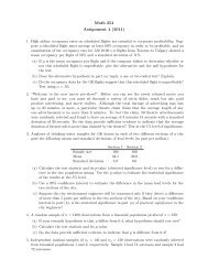
(d) The graph of i(t) is the following.
0.5
0.4
0.3
0.2
0.1
0.0
0.0
0.2
0.4
0.6
0.8
1.0
t
1.2
1.4
1.6
1.8
2.0
Observe that the current i(t) is continuous even though the voltage is
discontinuous at t = 1.
12. We have
δ ε (t − a) = 1 ε U(t − a) − 1 U(t − (a + ε)).
ε

2.5. CONVOLUTION 33
(a) Taking Laplace transform, we get
L {δ ε (t − a)} = 1 ε
= e−as
s
( e
−as
)
− 1 s ε
( 1 − e
−εs
ε
( ) e
−(a+ε)s
)
.
(b) We will use l’Hôpital’s rule to compute the limit.
lim L {δ ε(t − a)} = lim
ε→0
ε→0
e −as
= e−as
s
= e−as
s
= e−as
✁ s ( ✁ s)
= e −as
s
( ) 1 − e
−εs
s ε
(
1 − e −εs )
lim
ε→0 ε
(
se −εs )
lim
ε→0 1
2.5 Convolution
1. We will use the convolution theorem.
(a) L { 1 ∗ t 4} = L {1} L { t 4} = 1 s
(b) Observe that
∫ t
0
L {f(t) ∗ g(t)} = F (s)G(s)
cos θ dθ = 1 ∗ cos t.
(c) L {e t ∗ sin t} = L {e t } L {sin t} =
( ) 4!
s 5 = 24
s 6
{∫ t
}
L cos θ dθ = L {1 ∗ cos t}
0
= L {1} L {cos t}
= 1 (
✁ s )
✁ s s 2 + 1
=
1
s 2 + 1
( ) ( )
1 1
s − 1 s 2 =
+ 1
1
(s − 1)(s 2 + 1)

34 CHAPTER 2. SOLUTIONS
(d) Observe that
∫ t
0
cos θ sin(t − θ) dθ = cos t ∗ sin t.
{∫ t
}
L cos θ sin(t − θ) dθ
0
= L {cos t ∗ sin t}
( s
=
s 2 + 1
=
s
(s 2 + 1) 2
) ( 1
s 2 + 1
)
2. We will use the convolution theorem.
L −1 {F (s)G(s)} = f(t) ∗ g(t) =
∫ t
0
f(θ)g(t − θ) dθ
(a) Let F (s) = 1 s
and G(s) =
1
s − 1 , then
f(t) = L −1 {F (s)} = 1 and g(t) = L −1 {G(s)} = e t .
Therefore,
{ }
L −1 1
= L −1 {F (s)G(s)}
s(s − 1)
= f(t) ∗ g(t)
= 1 ∗ e t
=
∫ t
0
e θ dθ
= e θ∣ ∣ t 0
= e t − 1.
(b) Let F (s) = 1
s + 1
and G(s) =
1
s − 3 , then
f(t) = L −1 {F (s)} = e −t and g(t) = L −1 {G(s)} = e 3t .

2.5. CONVOLUTION 35
Therefore,
{
}
L −1 1
= L −1 {F (s)G(s)}
(s + 1)(s − 3)
= f(t) ∗ g(t)
= e −t ∗ e 3t
=
∫ t
0
e −(t−θ) e 3θ dθ
∫ t
= e −t e 4θ dθ
0
( )∣ e
= e −t 4θ ∣∣∣
t
4
0
( e
= e −t 4t )
− 1
4
= e3t − e −t
.
4
(c) Let F (s) = 1 s
and G(s) =
1
s 2 + 1 , then
f(t) = L −1 {F (s)} = 1 and g(t) = L −1 {G(s)} = sin t.
Therefore,
{ }
L −1 1
s(s 2 = L −1 {F (s)G(s)}
+ 1)
= f(t) ∗ g(t)
= 1 ∗ sin t
=
∫ t
0
sin θ dθ
t
= − cos θ
∣
0
= 1 − cos t.
(d) Let F (s) = 1 s and G(s) = 1
s(s 2 + 1) , then
f(t) = L −1 {F (s)} = 1 and g(t) = L −1 {G(s)} = 1 − cos t.

36 CHAPTER 2. SOLUTIONS
Therefore,
{ }
L −1 1
s 2 (s 2 = L −1 {F (s)G(s)}
+ 1)
= f(t) ∗ g(t)
= 1 ∗ (1 − cos t
=
∫ t
0
1 − cos θ dθ
= (θ − sin θ)
∣
= t − sin t.
t
0
3. Since L {sin t} = 1
s 2 + 1 , then
{ }
L −1 1
(s 2 + 1) 2 = sin t ∗ sin t =
By using the identity
sin α sin β = 1 2
with α = θ and β = t − θ, we get
Therefore,
sin θ sin(t − θ) = 1 2
∫ t
0
sin θ sin(t − θ) dθ
(
cos(α − β) − cos(α + β)
)
(
cos(θ − (t − θ)) − cos(θ + (t − θ))
)
= 1 2(
cos(2θ − t) − cos t
)
.
{ }
L −1 1
(s 2 + 1) 2 = 1 ∫ t
(cos(2θ − t) − cos t) dθ
2 0
= 1 ( )∣ sin(2θ − t) ∣∣∣
t
− θ cos t
2 2
0
= 1 ( ) sin t
2 2 − t cos t − 1 ( sin(−t)
2 2
= 1 (sin t − t cos t)
2
We can now apply the scaling property
L {f(ωt)} = 1 ω F ( s
ω
)
)
− 0

2.5. CONVOLUTION 37
to the function f(t) = 1 2
(sin t − t cos t) to get
⎛
⎞
{ }
1
L
2 (sin ωt − ωt cos ωt) = 1 ⎜ 1 ⎟
⎝( ω ( s
) ) 2 2 ⎠
ω + 1
We can conclude that
4. First observe that
{ }
L −1 1
(s 2 + ω 2 ) 2 =
∫ t
The equation is then equivalent to
0
=
ω 3
(s 2 + ω 2 ) 2 .
sin ωt − ωt cos ωt
2ω 3 .
e −θ f(t − θ) dθ = e −t ∗ f(t).
f(t) = t + e 2t + e −t ∗ f(t).
Take Laplace transform on both sides to get
Solve for F (s) to get
Using partial fractions, we obtain
Therefore,
F (s) = 1 s 2 + 1
s − 2 + F (s)
s + 1 .
F (s) = 1 s 2 + 1 s 3 + s + 1
s(s − 2)
s + 1
s(s − 2) = −1/2 + 3/2
s s − 2 .
F (s) = 1 s 2 + 1 s 3 − 1 2
( ) 1
+ 3 ( ) 1
s 2 s − 2
Taking the inverse Laplace transform gives the answer.
f(t) = t + t2 2 − 1 2 + 3 2 e2t
5. The equation is of the form
f(t) ∗ f(t) = t 3 .

38 CHAPTER 2. SOLUTIONS
Take Laplace transform to get
F (s) · F (s) = F (s) 2 = 6 s 4 =⇒ F (s) = ± √
6
s 2 .
By taking the inverse Laplace transform we obtain the two answers
f(t) = ± √ 6t.
6. First observe that
∫ t
The equation is then equivalent to
0
e −2θ y(t − θ) dθ = e −2t ∗ y(t).
y ′ (t) + e −2t ∗ y(t) = 1.
Since y(0) = 0, we can take Laplace transform on both sides to get
Solve for Y (s) to get
Using partial fractions, we deduce
sY (s) + Y (s)
s + 2 = 1 s .
Y (s) = s + 2
s(s + 1) 2 .
Y (s) = 2 s − 2
s + 1 − 1
(s + 1) 2 .
Taking the inverse Laplace transform gives the answer.
y(t) = 2 − 2e −t − te −t

Appendix A
Formulas and Properties
A.1 Table of Laplace Transforms
f(t) L {f(t)} = F (s) f(t) L {f(t)} = F (s)
1
1
s
e at 1
s − a
t n n!
s n+1 e at t n n!
(s − a) n+1
sin ωt
e at sin ωt
t sin ωt
ω
s 2 + ω 2
cos ωt
ω
(s − a) 2 + ω 2 e at cos ωt
2ωs
(s 2 + ω 2 ) 2 t cos ωt
s
s 2 + ω 2
s − a
(s − a) 2 + ω 2
s 2 − ω 2
(s 2 + ω 2 ) 2
sin ωt − ωt cos ωt
2ω 3 1
(s 2 + ω 2 ) 2 U(t − a)
e −as
s
δ(t) 1 δ(t − a) e −as
39

40 APPENDIX A. FORMULAS AND PROPERTIES
A.2 Properties of Laplace Transforms
1. Definition
F (s) = L {f(t)} =
∫ ∞
0
e −st f(t) dt
2. Linearity
L {αf(t) + βg(t)} = αL {f(t)} + βL {g(t)}
3. Time differentiation
L {f ′ (t)} = sF (s) − f(0) L {f ′′ (t)} = s 2 F (s) − sf(0) − f ′ (0)
{ }
L f (n) (t) = s n F (s) − s n−1 f(0) − · · · − f (n−1) (0)
4. Frequency differentiation
L {t n f(t)} = (−1) n F (n) (s)
5. Time shift
L {f(t) U(t − a)} = e −as L {f(t + a)}
L −1 { e −as F (s) } = f(t − a) U(t − a)
6. Frequency shift
L { e at f(t) } = F (s − a)
7. Convolution
f(t) ∗ g(t) =
∫ t
0
f(θ)g(t − θ) dθ =⇒ L {f(t) ∗ g(t)} = F (s)G(s)
8. Integration
{∫ t
}
L f(θ) dθ = F (s)
0
s
9. Periodic function
f(t) has period T =⇒ L {f(t)} =
∫
1 T
1 − e −sT
0
e −st f(t) dt
10. Scaling
L {f(ωt)} = 1 ω F ( s
ω
)

A.3. TRIGONOMETRIC IDENTITIES 41
A.3 Trigonometric Identities
1. Pythagorean Identities
sin 2 θ + cos 2 θ = 1 1 + tan 2 θ = sec 2 θ 1 + cot 2 θ = csc 2 θ
2. Symmetry Identities
sin(−θ) = − sin θ cos(−θ) = cos θ tan(−θ) = − tan θ
3. Sum and Difference Identities
sin(α + β) = sin α cos β + cos α sin β
cos(α + β) = cos α cos β − sin α sin β
tan(α + β) =
tan α + tan β
1 − tan α tan β
sin(α − β) = sin α cos β − cos α sin β
cos(α − β) = cos α cos β + sin α sin β
tan(α − β) =
tan α − tan β
1 + tan α tan β
4. Double-Angle Identities
cos 2θ = cos 2 θ − sin 2 θ
5. Power-Reducing Identities
sin 2θ = 2 sin θ cos θ
= 1 − 2 sin 2 θ tan 2θ = 2 tan θ
1 − tan 2 θ
= 2 cos 2 θ − 1
cos 2 θ =
1 + cos 2θ
2
sin 2 θ =
1 − cos 2θ
2
6. Product-To-Sum Identities
sin α cos β = 1 ( )
sin(α − β) + sin(α + β)
2
sin α sin β = 1 ( )
cos(α − β) − cos(α + β)
2
cos α cos β = 1 ( )
cos(α − β) + cos(α + β)
2

42 APPENDIX A. FORMULAS AND PROPERTIES

Appendix B
Partial Fractions
B.1 Partial Fractions
Consider a function F (s) expressed as a quotient of two polynomials
F (s) = P (s)
Q(s)
where Q(s) has a degree smaller than the degree of P (s). The method of partial
fractions can be summarized as follows.
1. Completely factor Q(s) into factors of the form
(ps + q) m and (as 2 + bs + c) n
where as 2 + bs + c is an irreducible quadratic.
2. For each factor of the form (ps + q) m , the partial fractions decomposition
must include the following m terms.
A 1
ps + q + A 2
(ps + q) 2 + · · · + A m
(ps + q) m .
3. For each factor of the form (as 2 + bs + c) n , the partial fractions decomposition
must include the following n terms.
B 1 s + C 1
as 2 + bs + c + B 2s + C 2
(as 2 + bs + c) 2 + · · · + B ns + C n
(as 2 + bs + c) n .
4. Find the values of all the constants.
43

44 APPENDIX B. PARTIAL FRACTIONS
B.2 Cover-up Method
There are several different ways to determine the constants in a partial fractions
decomposition. When the denominator has distinct roots, we can use the
cover-up method. Let’s illustrate it with some examples.
Example 1. Consider
s 2 + 5s + 4
(s − 1)(s − 3)(s + 2) = A
s − 1 +
B
s − 3 +
C
s + 2
(B.1)
To find A, we could use the following two steps.
1. Multiply both sides of equation (B.1) by (s − 1)(s − 3)(s + 2) to obtain
s 2 + 5s + 4 = A(s − 3)(s + 2) + B(s − 1)(s + 1) + C(s − 1)(s − 3).
2. Set s = 1 and solve for A.
1 + 5 + 4 = A(−2)(3) + 0 + 0 =⇒ A = − 5 3
The cover-up method combines these two steps in a single one as follows. To
find A, we cover up (s − 1) and set s = 1 in the left-hand side of (B.1).
s 2 + 5s + 4
A =
✘(s ✘ − ✘
= − 5
1) (s − 3)(s + 2) ∣ 3
s=1
We can find constants B and C in the same way. To find B, we cover up (s − 3)
and set s = 3.
s 2 + 5s + 4
B =
(s − 1) ✘✘ (s − ✘
= 14
3) (s + 2) ∣ 5
s=3
To find C, we cover up (s + 2) and set s = −2.
s 2 + 5s + 4
C =
(s − 1)(s − 3) ✘✘ (s + ✘
= − 2
2) ∣ 15
s=−2

B.2. COVER-UP METHOD 45
If the denominator includes irreducible quadratics terms, the cover-up method
works if we use complex numbers as in the following examples.
Example 2. Consider
s
(s + 1)(s 2 + 4) = A
s + 1 + Bs + C
s 2 + 4 .
Since s + 1 = 0 if s = −1, then
s
A =
✘(s ✘ + ✘
= − 1
1) (s 2 + 4) ∣ 5
s=−1
Since s 2 + 4 = 0 if s = 2j, then
(Bs + C)| s=2j =
s
(s + 1) ✘(s 2 ✘✘ +
✘
4)
∣
∣
s=2j
2Bj + C =
2j
1 + 2j
( )
2j 1 − 2j
=
(1 + 2j) 1 − 2j
= 2j + 4 .
5
The real and imaginary parts of the complex numbers on both sides are equal.
We conclude that
2B = 2 5 =⇒ B = 1 5
and
C = 4 5 .

46 APPENDIX B. PARTIAL FRACTIONS
Example 3. Consider
F (s) =
By completing the square, we get
s 2
(s + 2)(s 2 + 6s + 13) .
s 2 + 6s + 13 = (s + 3) 2 + 4.
We can look for a partial fractions decomposition of F (s) in the form
s 2
(s + 2)(s 2 + 6s + 13) = A B(s + 3) + C
+
s + 2 (s + 3) 2 + 4 .
Observe that by using B(s+3)+C instead Bs+C, we make it a little bit easier
since we do not have to solve a linear system to find B and C.
Since s + 2 = 0 if s = −2, then
s 2
A =
✘(s ✘ + ✘
= 4
2) (s 2 + 6s + 13) ∣ 5
s=−2
Since s 2 + 6s + 13 = (s + 3) 2 + 4 = 0 if s = −3 + 2j, then
(B(s + 3) + C)| s=−3+2j =
2Bj + C =
2Bj + C =
s 2
✭
(s + 2) ✭✭✭✭✭
(s 2 + 6s + 13)
(−3 + 2j)2
(−3 + 2j) + 2
= 5 − 12j
−1 + 2j
= 5 − 12j
−1 + 2j
2j − 29
.
5
( ) −1 − 2j
−1 − 2j
∣
∣
s=−3+2j
The real and imaginary parts of the complex numbers on both sides are equal.
We conclude that
2B = 2 5 =⇒ B = 1 5
and
C = − 29
5 .

Bibliography
[1] Johnson W.E., Kohler L., Elementary Differential Equations with Boundary
Value Problems, Second Edition, Addison Wesley, (2006).
[2] Simmons George F., Differential Equations with Applications and Historical
Notes, Second Edition, McGraw Hill, (1991).
[3] Wikipedia contributors, Laplace transform, Wikipedia, The Free Encyclopedia,
http://en.wikipedia.org/wiki/Laplace transform, (May
2006).
[4] Washington Allyn J., Basic Technical Mathematics with Calculus, Eight
Edition, Addison Wesley, (2005).
[5] Weisstein Eric W., Laplace Transform, From MathWorld – A Wolfram
Web Resource, http://mathworld.wolfram.com/LaplaceTransform.
html, (May 2006).
[6] Zill Dennis G., A First Course in Differential Equations, Eight Edition,
Brooks/Cole, (2005).
47