Structural Verification and Modeling of a Tension Cone Inflatable ...
Structural Verification and Modeling of a Tension Cone Inflatable ...
Structural Verification and Modeling of a Tension Cone Inflatable ...

You also want an ePaper? Increase the reach of your titles
YUMPU automatically turns print PDFs into web optimized ePapers that Google loves.
51st AIAA/ASME/ASCE/AHS/ASC Structures, <strong>Structural</strong> Dynamics, <strong>and</strong> Materials Conference18th<br />
12 - 15 April 2010, Orl<strong>and</strong>o, Florida<br />
AIAA 2010-2830<br />
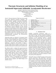
<strong>Structural</strong> <strong>Verification</strong> <strong>and</strong> <strong>Modeling</strong> <strong>of</strong> a <strong>Tension</strong> <strong>Cone</strong><br />
<strong>Inflatable</strong> Aerodynamic Decelerator<br />
Christopher L. Tanner *<br />
Georgia Institute <strong>of</strong> Technology, Atlanta, GA 30332-0150<br />
Juan R. Cruz †<br />
NASA Langley Research Center, Hampton, VA 23681-2199<br />
<strong>and</strong><br />
Robert D. Braun ‡<br />
Georgia Institute <strong>of</strong> Technology, Atlanta, GA 30332-0150<br />
<strong>Verification</strong> analyses were conducted on membrane structures pertaining to a tension<br />
cone inflatable aerodynamic decelerator using the analysis code LS-DYNA. The responses <strong>of</strong><br />
three structures - a cylinder, torus, <strong>and</strong> tension shell - were compared against linear theory<br />
for various loading cases. Stress distribution, buckling behavior, <strong>and</strong> wrinkling behavior<br />
were investigated. In general, agreement between theory <strong>and</strong> LS-DYNA was very good for<br />
all cases investigated. These verification cases exposed the important effects <strong>of</strong> using a linear<br />
elastic liner in membrane structures under compression. Finally, a tension cone wind tunnel<br />
test article is modeled in LS-DYNA for which preliminary results are presented. Unlike data<br />
from supersonic wind tunnel testing, the segmented tension shell <strong>and</strong> torus experienced<br />
oscillatory behavior when subjected to a steady aerodynamic pressure distribution. This<br />
work is presented as a work in progress towards development <strong>of</strong> a fluid-structures<br />
interaction mechanism to investigate aeroelastic behavior <strong>of</strong> inflatable aerodynamic<br />
decelerators.<br />
b = arc length <strong>of</strong> wrinkled region<br />
B 2 = tension shell shape factor<br />
c = torus radius ratio (r m /r M )<br />
C p = pressure coefficient<br />
E = elastic modulus<br />
F cr = critical buckling load<br />
G = shear modulus<br />
l = length<br />
M = applied moment<br />
p = internal pressure<br />
p a = aerodynamic pressure distribution<br />
p 0 = uniform pressure distribution<br />
P = force due to internal pressure (pπr 2 )<br />
r = radius or tension shell radial coordinate<br />
r b = tension shell base radius<br />
= minor torus radius<br />
r m<br />
Nomenclature<br />
* Graduate Research Assistant, Daniel Guggenheim School <strong>of</strong> Aerospace Engineering, AIAA Student Member,<br />
christopher.tanner@gatech.edu<br />
† Aerospace Engineer, Atmospheric Flight <strong>and</strong> Entry Systems Branch, AIAA Member, Juan.R.Cruz@nasa.gov<br />
‡ Associate Pr<strong>of</strong>essor, Daniel Guggenheim School <strong>of</strong> Aerospace Engineering, AIAA Fellow,<br />
robert.braun@ae.gatech.edu<br />
1<br />
American Institute <strong>of</strong> Aeronautics <strong>and</strong> Astronautics<br />
This material is declared a work <strong>of</strong> the U.S. Government <strong>and</strong> is not subject to copyright protection in the United States.
M<br />
t<br />
x,y,z<br />
z<br />
= major torus radius<br />
= material thickness<br />
= Cartesian coordinates for cylinder<br />
= tension shell axial coordinate<br />
α = tension shell stress ratio (σ c /σ m )<br />
ε c = circumferential strain<br />
κ = cylinder curvature due to load<br />
φ = angle measurement around torus cross-section<br />
ν = Poisson’s ratio<br />
σ 0 = stress at base <strong>of</strong> tension shell<br />
σ c = circumferential stress<br />
σ l = longitudinal stress<br />
= meridional stress<br />
σ m<br />
FSI<br />
IAD<br />
LSTC<br />
= Fluid-Structures Interaction<br />
= <strong>Inflatable</strong> Aerodynamic Decelerator<br />
= Livermore S<strong>of</strong>tware Technology Corporation<br />
I<br />
I. Introduction<br />
nflatable aerodynamic decelerator (IAD) designs, such as the tension cone shown in Figure 1, will require<br />
fluid-structure interaction (FSI) analyses to appropriately assess structural response at relevant aerodynamic<br />
conditions <strong>and</strong> scales. However, given the complexity <strong>of</strong> FSI, it is <strong>of</strong>ten useful to analyze portions <strong>of</strong> the problem<br />
under simplified conditions rather than immediately attempting to analyze the full problem. This process can lead to<br />
a better underst<strong>and</strong>ing <strong>of</strong> the underlying physics <strong>and</strong> the behavior <strong>of</strong> the computational tools used to model those<br />
physics.<br />
Figure 1. <strong>Tension</strong> cone IAD (figure from Ref. 1).<br />
A tension cone IAD consists <strong>of</strong> a shell <strong>of</strong> revolution, referred to as a tension shell attached at one end to the<br />
forebody <strong>of</strong> a blunt entry vehicle, <strong>and</strong> at the other end to a pressurized, toroidal structural member. The tension shell<br />
is intentionally shaped to carry only tensile loads in the meridional <strong>and</strong> circumferential directions while transferring<br />
compressive loads to the torus. <strong>Inflatable</strong> aerodynamic decelerators such as the tension cone are meant for<br />
supersonic deceleration, particularly in thin atmospheres, <strong>and</strong> will likely be constructed from high-strength textile<br />
materials with impermeable liners or coatings.<br />
This document summarizes a verification <strong>of</strong> the analysis code LS-DYNA 2 , developed by the Livermore S<strong>of</strong>tware<br />
Technology Corporation (LSTC), as applied to structures relevant to tension cone IADs. The tension cone is reduced<br />
to simple geometries -- a cylinder, torus, <strong>and</strong> tension shell -- which have well-understood static behavior. Analytical<br />
relationships that predict stress distributions, buckling loads, <strong>and</strong> wrinkling behavior for these shapes are used as a<br />
benchmark for comparison with LS-DYNA. These simple cases bring out the effects <strong>of</strong> particular modeling<br />
parameters in LS-DYNA, with various geometries <strong>and</strong> loading scenarios exercising different aspects <strong>of</strong> the code.<br />
Following verification, a preliminary structural analysis is performed on a tension cone IAD that is representative <strong>of</strong><br />
a fully inflatable tension cone wind tunnel model tested in the 10- by 10-ft Supersonic Wind Tunnel at the NASA<br />
2<br />
American Institute <strong>of</strong> Aeronautics <strong>and</strong> Astronautics
Glenn Research Center. 1 This work represents the initial structural verification <strong>of</strong> LS-DYNA, as part <strong>of</strong> a larger FSI<br />
effort intended to predict the aeroelastic behavior <strong>of</strong> IADs in supersonic flowfields.<br />
II. Textile <strong>Modeling</strong> Parameters<br />
Unless otherwise stated, all <strong>of</strong> the following verification cases were performed using the same material <strong>and</strong> finite<br />
element parameters stated here to maintain consistency across all solutions. The textile portion <strong>of</strong> each structure was<br />
modeled using membrane shell elements 0.01315 inches thick. The mat_fabric material model was used assuming<br />
the following isotropic properties: elastic modulus (E) <strong>of</strong> 387.7 ksi, Poisson’s ratio (ν) <strong>of</strong> 0.3, <strong>and</strong> shear modulus (G)<br />
determined from G = 0.5E / (1+ν). The fabric material model invokes an alternate membrane element algorithm<br />
using one through-thickness integration point regardless <strong>of</strong> what is specified in the section_shell keyword.<br />
LSTC recommends adding a “liner” to help stabilize membrane elements that have gone into compression. The<br />
liner is a linear elastic material that augment the element’s original material definition, effectively increasing tensile<br />
stiffness <strong>and</strong> making compressive stiffness non-zero, but maintaining zero bending stiffness in the element. Since<br />
the verification cases involve matching analytic theories (which assume zero compressive stiffness) <strong>and</strong> are<br />
pseudo-static, a liner was omitted from the models. LSTC also recommends adding at least 5% Rayleigh damping<br />
(corresponding to 5% <strong>of</strong> the critical damping value) to increase the stability <strong>of</strong> membrane elements. However,<br />
loaded elements still appeared to experience oscillatory behavior with low damping. Thus, in the attempt to obtain<br />
pseudo-static results, damping was increased to 100% <strong>of</strong> critical damping. The LS-DYNA keyword parameters<br />
described above are presented in card format in Table 1.<br />
Table 1. LS-DYNA keyword parameters for fabric portion <strong>of</strong> all verification cases.<br />
*SECTION_SHELL<br />
secid elform shrf nip propt qr/irid icomp setyp<br />
1 5 1 1 1 0 0 1<br />
t1 t2 t3 t4 nloc marea id<strong>of</strong> edgset<br />
0.01315 0.01315 0.01315 0.01315 0 0 0 0<br />
*MAT_FABRIC<br />
mid ro ea eb ec prba prca prcb<br />
1 1.0544E-4 387705 0 0 0.3 0 0<br />
gab gbc gca cse el prl lratio damp<br />
0 0 0 1 0 0 0 1.0<br />
aopt flc fac ela lnrc form fvopt tsrfac<br />
0 0 0 0 0 0 0 0<br />
xp yp zp a1 a2 a3 xd xl<br />
0 0 0 0 0 0 0 0<br />
All cases were solved explicitly using the double precision, symmetric multiprocessor version <strong>of</strong> the LS-DYNA<br />
v971, release 4.2. Generally explicit codes are intended for dynamic problems that have time dependence <strong>and</strong> are<br />
not generally used for pseudo-static problems. LS-DYNA does have an implicit solving routine that is more suited<br />
for static problems. However, membrane elements are not implemented in LS-DYNA’s implicit routine, which<br />
immediately precludes its use for this study. To effectively use an explicit solver for the following pseudo-static<br />
cases: (a) loads must be applied smoothly, (b) energy balance must be monitored to ensure that the systems energy is<br />
due almost entirely to internal energy, not kinetic energy, <strong>and</strong> (c) damping must be used with care to create a static<br />
solution in a short period <strong>of</strong> time without significantly influencing the end result.<br />
III. Column Buckling <strong>and</strong> Membrane Wrinkling<br />
Two circular cylinders were constructed to perform buckling <strong>and</strong> wrinkling verification <strong>of</strong> LS-DYNA. For a<br />
tension cone IAD, buckling prediction is particularly important as it is a critical collapse mode which drives the<br />
required torus internal pressure <strong>and</strong> consequently its mass. For the same reasons, wrinkling is an important response.<br />
Cylinder geometry <strong>and</strong> nomenclature are given in Figure 2. The Cartesian coordinate system originates from the<br />
base <strong>of</strong> the cylinder along the axis <strong>of</strong> symmetry. The radius for all cylinders is 1.5 inches.<br />
3<br />
American Institute <strong>of</strong> Aeronautics <strong>and</strong> Astronautics
l<br />
! c<br />
p<br />
x<br />
! l<br />
r<br />
z<br />
y<br />
t<br />
x,y,z<br />
r<br />
p<br />
t<br />
l<br />
σ l<br />
σ c<br />
Cartesian coordinate system<br />
radius<br />
internal pressure<br />
membrane thickness<br />
length<br />
longitudinal stress<br />
circumferential stress<br />
Figure 2. Cylinder geometry <strong>and</strong> nomenclature.<br />
A. Column Buckling<br />
A column 45 inches in length was modeled to investigate buckling behavior. Column end caps were modeled as<br />
stiff plates. The bottom cap was constrained in translation but permitted to rotate only about the x-axis; the top cap<br />
was only permitted to translate along the z-axis <strong>and</strong> rotate about the x-axis. An internal pressure <strong>of</strong> 200 psi was<br />
imposed to achieve a configuration that exhibited global buckling while retaining tensile longitudinal stress when<br />
buckled. The radius <strong>of</strong> the un-inflated shape was reduced to ensure that the final, inflated radius was close to 1.5<br />
inches. Fichter 3 approximated the critical buckling load <strong>of</strong> a column with membrane walls subject to internal<br />
pressure assuming the cylinder walls remain in tension <strong>and</strong> the column’s cross-section remains circular throughout.<br />
Fichter’s relationship for the critical buckling load is<br />
( )( pπr 2 +Gπrt)<br />
F cr<br />
= EIπ2 l −2<br />
EIπ 2 l −2 +pπr 2 +Gπrt<br />
(1)<br />
One issue common to buckling analysis using finite element analysis is that imperfection needs to be introduced<br />
into the model in order to recover an appropriate buckling load. Thus, for this model, imperfection was introduced as<br />
an applied moment couple at both € ends <strong>of</strong> the column at various magnitudes. Buckling results are given in Figure 3.<br />
Figure 3b shows that the buckling load with no end moment overshoots Fichter’s value <strong>and</strong> experiences substantial<br />
oscillation after buckling has occurred. The addition <strong>of</strong> small moments at the ends <strong>of</strong> the columns decrease the<br />
buckling load overshoot <strong>and</strong> subsequent oscillations. Oscillation is due to the release <strong>of</strong> potential energy after<br />
buckling. A 10 Hz Butterworth filter was applied to results to extract a pseudo-static buckling load as shown in<br />
Figure 3b. Even though the peak buckling load varies considerably with the applied moment, the steady-state<br />
buckled load appears to be within about 4% <strong>of</strong> that predicted by Fichter’s theory for all cases.<br />
B. Membrane Wrinkling – Cylinder Compresion<br />
A cylinder six inches in length was modeled to investigate its wrinkling response (i.e., zero wall stress<br />
condition). The column was subjected to 20 psi <strong>of</strong> internal pressure. Boundary conditions were a fixed lower end<br />
cap, <strong>and</strong> an upper end cap that was only allowed to translate axially. In Figure 4 the end cap externally applied force<br />
versus stroke response is plotted. The black line represents axial force due to internal pressure, where internal<br />
pressure is linearly dependent on the cylinder’s volume, which varies as stroke increases. For a cylinder with<br />
membrane walls, the externally applied force should be equal to the internal force after the walls have wrinkled.<br />
Indeed, LS-DYNA recovers this force when no liner is present after the cylinder walls have wrinkled. Wall<br />
oscillation occurs just after wrinkling <strong>and</strong> ceases when the cylinder compresses into a stable configuration with<br />
walls deflected outward, as in Figure 5c.<br />
4<br />
American Institute <strong>of</strong> Aeronautics <strong>and</strong> Astronautics
Force (lb)<br />
400<br />
350<br />
300<br />
250<br />
200<br />
150<br />
0.0 in-lb<br />
100<br />
1.0 in-lb<br />
50<br />
6.0 in-lb<br />
Theory<br />
0<br />
0.5 0.6 0.7 0.8 0.9 1.0 1.1 1.2 1.3 1.4 1.5<br />
Time (s)<br />
400<br />
350<br />
300<br />
(b) 100 Hz response<br />
(a) Contours <strong>of</strong> σ l<br />
Force (lb)<br />
250<br />
200<br />
150<br />
0.0 in-lb<br />
100<br />
1.0 in-lb<br />
50<br />
6.0 in-lb<br />
Theory<br />
0<br />
0.5 0.6 0.7 0.8 0.9 1.0 1.1 1.2 1.3 1.4 1.5<br />
Time (s)<br />
(c) Filtered response<br />
Figure 3. Column buckling response for various moment couples.<br />
250<br />
200<br />
wall<br />
wrinkles<br />
Force (lb)<br />
150<br />
100<br />
50<br />
wall<br />
oscillation<br />
stable<br />
compression<br />
p!r 2<br />
0% liner<br />
10% liner<br />
0<br />
20% liner<br />
0.0 0.1 0.2 0.3 0.4<br />
Stroke (in)<br />
Figure 4. <strong>Structural</strong> response <strong>of</strong> a short cylinder using for various liner thicknesses.<br />
5<br />
American Institute <strong>of</strong> Aeronautics <strong>and</strong> Astronautics
(a) Inflated, pre-loaded (b) Wall oscillation (c) Stable compression<br />
Figure 5. Cylinder buckling progression.<br />
The addition <strong>of</strong> a linear elastic liner significantly increases the amount <strong>of</strong> external force required for a given stroke<br />
after the cylinder walls have wrinkled. Reaction force is a function <strong>of</strong> both the internal pressure as well as the<br />
compressive load carried by the cylinder walls. Greater external force is required during compression since the liner,<br />
despite its small elastic modulus <strong>and</strong> thickness with respect to the base material, has compressive strength <strong>and</strong> will<br />
carry a non-negligible amount <strong>of</strong> load. The liner is defined by an elastic modulus 10% <strong>of</strong> the base material<br />
(E liner = 0.10E) <strong>and</strong> a Poisson’s ratio equal to that <strong>of</strong> the base material. Liner thickness is a fraction <strong>of</strong> the base<br />
material’s thickness (i.e., a 10% liner corresponds to t liner = 0.10t).<br />
C. Membrane Wrinkling – Cylinder Bending<br />
A cylinder six inches in length was subjected to 30 psi <strong>of</strong> internal pressure <strong>and</strong> a linearly increasing moment<br />
couple. The ends, modeled as rigid shells, were assigned boundary conditions similar to the column in Section II.A.<br />
Stein <strong>and</strong> Hedgpeth 4 developed a relationship that relates an applied moment couple to the curvature <strong>of</strong> the column,<br />
effectively showing that a pressurized cylinder is able to maintain a stable, static configuration in a partially<br />
wrinkled state. This is an important result for the tension cone as it implies that a partially wrinkled configuration<br />
will continue to support load. * Figure 6 provides additional nomenclature <strong>and</strong> compares results against Stein <strong>and</strong><br />
Hedgepeth’s theory. In Figure 6a, the parameter b is an arc length, measured from the bottom <strong>of</strong> the cylinder at<br />
b = 0, to the edge <strong>of</strong> the wrinkled region, with a maximum length <strong>of</strong> b = πr; in other words, it is half <strong>of</strong> the total arc<br />
length <strong>of</strong> the wrinkled region.<br />
For the material established in Section II, LS-DYNA results almost exactly match theory. This test case also<br />
helps illustrate the liner explored in Section III.B. Figure 6c indicates that wrinkling response is approximately the<br />
same for all cases until b/πr = 1/2. The liner then begins to have a noticeable effect, requiring larger moments for a<br />
given curvature, despite its low modulus <strong>and</strong> thickness relative to the base material. These results illustrate that liner<br />
effects may be non-negligible when a structure is in a wrinkled condition. This corroborates the results in Section<br />
II.B <strong>and</strong> reinforces that implementing a liner must be done with care since the structural response may deviate from<br />
the actual response.<br />
* In Reference 4 a photograph is shown <strong>of</strong> a cylinder in just such a partially wrinkled configuration, showing that<br />
this is a physically possible state.<br />
6<br />
American Institute <strong>of</strong> Aeronautics <strong>and</strong> Astronautics
(a) Column post-buckling nomenclature (figure from Ref. 4)<br />
1.0<br />
M/Pr<br />
0.9<br />
0.8<br />
0.7<br />
0.6<br />
0.5<br />
0.4<br />
0.3<br />
0.2<br />
0.1<br />
0.0<br />
1/3<br />
1/6<br />
b/!r = 0<br />
1/2<br />
0% liner<br />
10% liner<br />
20% liner<br />
Theory<br />
0 2 4 6 8 10<br />
2!r 2 Et"/P<br />
2/3<br />
(b) Contours <strong>of</strong> σ l<br />
(c) Moment-curvature response to various liner<br />
thicknesses<br />
Figure 6. Column post-buckling results for various liner thicknesses.<br />
IV. Torus Stress Distribution<br />
For the tension cone IAD, a pressurized torus serves as a primary load-bearing member, reacting the<br />
compressive loads transmitted through the tension shell. Accurate prediction <strong>of</strong> the stress distribution <strong>of</strong> a torus<br />
translates directly into material requirements <strong>and</strong> mass estimation <strong>of</strong> the tension cone. 5 Torus geometry <strong>and</strong><br />
nomenclature is provided in Figure 7.<br />
t<br />
r m<br />
p<br />
r<br />
!"<br />
r M<br />
# c<br />
# m<br />
r M<br />
r m<br />
p<br />
t<br />
φ<br />
σ m<br />
σ c<br />
Figure 7. Torus geometry <strong>and</strong> nomenclature.<br />
major radius<br />
minor radius<br />
internal pressure<br />
thickness<br />
angle around cross-section<br />
meridional stress<br />
circumferential stress<br />
Linear theory for the stress distribution in a toroidal shell relies on the assumption that the major torus radius is<br />
much larger than the minor torus radius. 6 In this scenario, a section <strong>of</strong> the torus appears as a cylinder <strong>and</strong> the<br />
circumferential stress can be approximated as a constant value throughout the shell. For cases in which the torus<br />
!"<br />
radius ratio (c = r m /r M ) is not small, circumferential stress becomes nonlinear. S<strong>and</strong>ers 7 presents a nonlinear theory<br />
for accurately predicting torus stresses in both the meridional <strong>and</strong> circumferential directions.<br />
7<br />
American Institute <strong>of</strong> Aeronautics <strong>and</strong> Astronautics
Nondimensional Stress, !<br />
1.4<br />
1.2<br />
1.0<br />
0.8<br />
0.6<br />
Circumferential (! c )<br />
0.4<br />
Linear<br />
Meridional (! m )<br />
0.2 Nonlinear<br />
0.0<br />
LS-DYNA<br />
-90 -60 -30 0 30 60 90<br />
" (deg)<br />
(a) Contours <strong>of</strong> σ c<br />
(b) Normalized torus stress distribution<br />
Figure 8. Comparison <strong>of</strong> linear, nonlinear, <strong>and</strong> computational stress for c = 2/3. Stress is non-dimensionalized<br />
by the maximum linear stress in each direction.<br />
In Figure 8 solid lines represents analytical predictions in the meridional direction, dotted lines represents<br />
analytical predictions in the circumferential direction, with black being used for the linear theory <strong>and</strong> grey being<br />
used for the nonlinear theory. Discrete symbols represent LS-DYNA solutions. Figure 8 shows that finite element<br />
results are nearly identical to the nonlinear solution for both the circumferential <strong>and</strong> meridional stresses. However,<br />
linear theory in the circumferential direction predicts the incorrect behavior <strong>and</strong> differs from the nonlinear <strong>and</strong><br />
computational results by up to 18%.<br />
V. <strong>Tension</strong> Shell Stress Distribution<br />
The tension shell as discussed here is a conical structure as proposed by Anderson et. al. 8 for mass efficient<br />
decelerator concepts. The tension shell shape, given in Figure 9, can be obtained assuming a constant stress ratio<br />
(α = σ c /σ m ), a shape parameter, <strong>and</strong> an axisymmetric aerodynamic pressure distribution (p a ).<br />
r b<br />
r<br />
! m<br />
! c<br />
nose<br />
base<br />
p a<br />
Figure 9. <strong>Tension</strong> shell geometry <strong>and</strong> nomenclature.<br />
A. Boundary Conditions<br />
In modeling the tension shell for this verification study the nose <strong>and</strong> base perimeters <strong>of</strong> the tension shell are<br />
constrained from moving in the radial direction. A radial constraint at the nose <strong>and</strong> base implies that the<br />
circumferential strain, ε c , is zero at these edges. For the isotropic material used in this verification study<br />
ε c<br />
= σ c −νσ m<br />
E<br />
(2)<br />
However, since ε c = 0 at the boundaries <strong>of</strong> the tension shell, Equation (2) yields σ c /σ m = ν. The tension shell theory<br />
defines a tension shell by a constant stress ratio, σ c /σ m = α. Thus, in order for the verification case <strong>and</strong> tension shell<br />
€<br />
theory to agree, α = ν. Per Section II, the material properties used for this study assume ν = 0.3; as such, the tension<br />
shell shape used for this study is defined by a stress ratio <strong>of</strong> 0.3. In addition to these radial constraints, the nose is<br />
fully constrained in axial translation, but the base is allowed to translate axially.<br />
8<br />
American Institute <strong>of</strong> Aeronautics <strong>and</strong> Astronautics
B. Stress Distribution<br />
For analytic pressure distributions, such as a uniform or Newtonian distribution, the tension shell pr<strong>of</strong>ile <strong>and</strong><br />
subsequent stress state can be derived from the tension shell theory. For a uniform pressure distribution, meridional<br />
stress (σ m ) is a function <strong>of</strong> the stress at the tension shell base (σ 0 ) <strong>and</strong> circumferential stress is a prescribed fraction<br />
<strong>of</strong> the meridional stress (α). These relationships, from reference 8, are given in Equations (3) where B 2 is the tension<br />
shell shape factor <strong>and</strong> p 0 is a constant, uniform pressure.<br />
σ 0<br />
= p 0r b<br />
2B 2 t<br />
1−α<br />
⎛ r<br />
σ m<br />
=σ b<br />
⎞<br />
0 ⎜ ⎟<br />
(3)<br />
⎝ r ⎠<br />
σ c<br />
=ασ m<br />
For these analyses, a uniform mesh was prescribed on a tension shell defined by α = 0.3 <strong>and</strong> B 2 = 0.5. The tension<br />
shell coordinates were obtained using the procedure described in reference 8.<br />
€<br />
250<br />
200<br />
Meridional (! m )<br />
Theory<br />
LS-DYNA<br />
Stress, ! (psi)<br />
150<br />
100<br />
50<br />
Circumferential (! c )<br />
0<br />
0.2 0.3 0.4 0.5 0.6 0.7 0.8 0.9 1.0<br />
Normalized Radius, r /r b<br />
(a) contours <strong>of</strong> σ m<br />
(b) <strong>Tension</strong> shell stress distribution<br />
Figure 10. <strong>Tension</strong> shell stress distribution results for α = 0.3, B 2 = 0.5, <strong>and</strong> p 0 = 0.1 psi.<br />
Figure 10b shows that the meridional stresses predicted by LS-DYNA are well behaved <strong>and</strong> follow the linear theory<br />
solution almost exactly. The circumferential stresses predicted by LS-DYNA agree with the linear theory solution<br />
up to a r/r b <strong>of</strong> 0.7. After this point, finite element results deviate from the linear solution. It is likely that this<br />
deviation is due to deformation <strong>of</strong> the tension shell geometry in the LS-DYNA model as compared to the shape<br />
specified in the linear theory; quoting from reference 8: “It should be noted that the circumferential stress N θ is very<br />
sensitive to small changes in the shape in the vicinity <strong>of</strong> the base; this sensitivity may require special consideration<br />
in the vehicle design.” (p. 12). In general agreement between the linear theory <strong>and</strong> the nonlinear LS-DYNA results<br />
should improve when deformations are negligible, as p 0 approaches zero <strong>and</strong>/or in the limit <strong>of</strong> a very stiff tension<br />
shell. In performing the work presented here, the sensitivity <strong>of</strong> the results to the exact shape <strong>of</strong> the tension shell was<br />
also observed near the nose.<br />
VI. <strong>Tension</strong> <strong>Cone</strong> <strong>Structural</strong> Model<br />
The tension cone shown in Figure 11 was tested in the 10- by 10-ft Supersonic Wind Tunnel at the NASA Glenn<br />
Research Center. 1<br />
9<br />
American Institute <strong>of</strong> Aeronautics <strong>and</strong> Astronautics
textile, inflatable torus. The inflatable torus was fabricated using the same urethane-coated<br />
kevlar as the tension shell. Inflation <strong>of</strong> the torus was achieved through two tubes located at<br />
the 3 o’clock <strong>and</strong> 9 o’clock positions on the back <strong>of</strong> the model. The inflation tubes were also<br />
constructed using kevlar to provide flexibility <strong>and</strong> allow for the model to be easily stowed.<br />
Inflation<br />
Tube<br />
Tunnel Sting &<br />
Support Hardware<br />
<strong>Inflatable</strong><br />
Torus<br />
(a) Front view (photo from Ref. 1) Figure 54: Aft view <strong>of</strong> (b) the Back inflatable view tension (photo cone from model Ref.5) installed in the test section.<br />
Figure 11. <strong>Inflatable</strong> tension cone model.<br />
Two variations <strong>of</strong> the inflatable model were used during testing. Due to pre-test<br />
A continuous tension cone was approximated by a 16-sided polygon constructed from urethane-coated Kevlar ® concerns<br />
fabric. The purpose <strong>of</strong> the urethane coating about was the to tension eliminate shell fabric torquing porosity the flexible <strong>and</strong> permit torus <strong>and</strong> gore causing seams it to to be roll welded forward during<br />
together instead <strong>of</strong> sewn. The welding process involved butting two seam ends together with a second layer <strong>of</strong> the<br />
testing, a series <strong>of</strong> panels were added. These anti-torque panels, shown in Figure 55, ran<br />
material <strong>and</strong> heating until the urethane bonded all pieces together. To properly seal all seams <strong>and</strong> ensure structural<br />
integrity, the tension cone employed between from the one back <strong>and</strong> <strong>of</strong>four the inflatable layers <strong>of</strong> torus welded to thematerial base <strong>of</strong> the throughout rigid aeroshell. the model. During early A testing<br />
detailed finite element model consisting <strong>of</strong> over 16,000 elements was constructed <strong>of</strong> this tension cone model. The<br />
<strong>of</strong> these two variations <strong>of</strong> inflatable models, differences in shape <strong>and</strong><br />
colored regions in the mesh shown in Figure 12 capture the various material thicknesses. The Kevlar ® aerodynamics were<br />
fabric is<br />
modeled identically to the verification cases observed. except that As athe result, thickness the anti-torque is increased panelas modification appropriate. was The alsoinflation applied to tubes the semi-rigid<br />
<strong>and</strong> metallic hardware are fully constrained as this represents the mounting configuration in the wind tunnel.<br />
model <strong>and</strong> both variants (with <strong>and</strong> without panels) were tested at similar conditions.<br />
89<br />
(a) front view<br />
(b) back view<br />
Figure 12. Detailed finite element mesh <strong>of</strong> tension cone.<br />
Preliminary aeroelastic response <strong>of</strong> the tension cone was obtained by first pressurizing the torus to 50 psi <strong>and</strong> then<br />
imposing the aerodynamic pressure distribution shown in Figure 13 on the tension shell <strong>and</strong> torus. The applied<br />
pressure distribution was obtained from rigid tension cone testing in the Unitary Plan Wind Tunnel at NASA<br />
Langley Research Center. 1<br />
10<br />
American Institute <strong>of</strong> Aeronautics <strong>and</strong> Astronautics
2.0<br />
Pressure Coefficient, C p<br />
1.5<br />
1.0<br />
0.5<br />
0.0<br />
-0.5<br />
0.0 0.2 0.4 0.6 0.8 1.0<br />
Normalized Radial Location<br />
Figure 13. Pressure distribution at Mach 2.5, adapted from Ref 5.<br />
The tension shell vibrated in response to the applied load. Similarly, the torus appeared to flex <strong>and</strong> oscillate about<br />
the axis formed by the inflation tubes. In general, the tension cone exhibited an unsteady response to a steady<br />
aerodynamic load, which contrasts the steady behavior observed during wind tunnel testing. The addition <strong>of</strong> a 10%<br />
liner eliminated torus the motion, but the tension shell vibration remained. A snapshot <strong>of</strong> the tension cone’s<br />
deformation is shown in Figure 14 using contours <strong>of</strong> axial displacement.<br />
(a) front view<br />
(b) back view<br />
Figure 14. <strong>Tension</strong> cone contours <strong>of</strong> axial displacement.<br />
The presented results are very preliminary, as the applied pressure distribution remained constant even as the<br />
structure deformed. Damping will be necessary to eliminate the vibrations on the tension shell <strong>and</strong> recover the static<br />
behavior observed during the wind tunnel test. Additionally, the material properties used are those described in<br />
Section II, which result in a shear modulus <strong>of</strong> 150 ksi. In contrast, the actual Kevlar ® material is orthotropic <strong>and</strong><br />
testing indicates that the material may have a shear modulus closer to 5 ksi 9 , over an order <strong>of</strong> magnitude lower than<br />
the value used in this preliminary tension cone analysis.<br />
VII. Summary <strong>and</strong> Future Work<br />
Several basic geometries <strong>and</strong> loading scenarios were simulated using the finite element analysis code LS-DYNA.<br />
The analysis code was verified against known analytical theories, both linear <strong>and</strong> nonlinear, using a single material<br />
<strong>and</strong> a finite element definition that did not utilize a liner. A liner was introduced into the wrinkling analysis to<br />
11<br />
American Institute <strong>of</strong> Aeronautics <strong>and</strong> Astronautics
illustrate how it augments the structure’s stiffness in situations where the membrane is placed in compression.<br />
Finally, a 16-segment tension cone wind tunnel test article is modeled with finite element boundaries along seam<br />
boundaries. Preliminary analysis was performed on the tension cone using a representative, static aerodynamic<br />
pressure distribution. The tension cone exhibited unsteady behavior to a steady load, which contradicts the steady<br />
behavior observed during wind tunnel testing. Introduction <strong>of</strong> damping <strong>and</strong> more appropriate material properties into<br />
the model will be necessary to create a more accurate representation <strong>of</strong> wind tunnel results.<br />
This paper is presented as a work in progress. To further mature the tension cone structural model, implementation<br />
<strong>of</strong> oriented, orthotropic, nonlinear materials on simple models <strong>and</strong> validation <strong>of</strong> those models against experimental<br />
results will be required. Following a validation <strong>of</strong> nonlinear material models, work will begin on implementing the<br />
segmented tension cone structural model presented in Section VI in a fluid dynamics solver. Difficulties in this area<br />
involve mapping the aerodynamic <strong>and</strong> structural grids to each other as well as implementing a scheme to control<br />
grid stretching or remeshing as the structure deforms. Additionally, it is not known how much <strong>of</strong> the tension cone’s<br />
aft structure will need to be modeled to recover accurate pressures. Joint implementation <strong>of</strong> accurate structural<br />
response <strong>and</strong> accurate aerodynamic pressures, which change with structural deformation, will be required to recover<br />
tension cone wind tunnel behavior. The fluid-structure interaction mechanism described above will be used to<br />
validate structural response against the static aeroelastic shape <strong>of</strong> the tension cone at various angles <strong>of</strong> attack as well<br />
as buckling response <strong>of</strong> the tension cone as torus pressure is reduced.<br />
References<br />
1 Clark, I. G., Cruz, J. R., Hughes, M. F., Ware, J. S., Madlangbayan, A., Braun, R. D., “Aerodynamic <strong>and</strong> Aeroelastic<br />
Characteristics <strong>of</strong> a <strong>Tension</strong> <strong>Cone</strong> <strong>Inflatable</strong> Aerodynamic Decelerator,” AIAA Aerodynamic Decelerator Systems Technology<br />
Conference <strong>and</strong> Seminar, AIAA-2009-2967, May 2009.<br />
2 LS-DYNA Keyword User’s Manual, Version 971, Vol. I-II, May 2007.<br />
3 Fichter, W. B., “A Theory for Inflated Thin-Wall Cylindrical Beams,” NASA TN D-3466, 1966.<br />
4 Stein, M. <strong>and</strong> Hedgepeth, J. M., “Analysis <strong>of</strong> Partly Wrinkled Membranes,” NASA TN D-813, 1961.<br />
5 Clark, I. G., Aerodynamic Design, Analyses, <strong>and</strong> Validation <strong>of</strong> a Supersonic <strong>Inflatable</strong> Aerodynamic Decelerator, Ph.D.<br />
Dissertation, Georgia Institute <strong>of</strong> Technology, August 2008.<br />
6 Young, W., C., Roark’s Formulas for Stress <strong>and</strong> Strain, McGraw-Hill Companies, 2002, p. 593.<br />
7 S<strong>and</strong>ers, J. L. <strong>and</strong> Liepins, A., A., “Toroidal Membrane Under Internal Pressure,” AIAA Journal, Vol. 1, No. 9, September<br />
1963, pp. 2105-2110.<br />
8 Anderson, M. S., Robinson J. C., Bush, H. G., <strong>and</strong> Fralich, R. W., “A <strong>Tension</strong> Shell Structure for Application to Entry<br />
Vehicles,” NASA TN D-2875, 1965.<br />
9 Hutchings, A. L., Braun, R. D., Masuyama, K. “Experimental Determination <strong>of</strong> Material Properties for <strong>Inflatable</strong> Aeroshell<br />
Structures,” AIAA Aerodynamic Decelerator Systems Technology Conference <strong>and</strong> Seminar, AIAA-2009-2949, May 2009.<br />
12<br />
American Institute <strong>of</strong> Aeronautics <strong>and</strong> Astronautics