Course on Model Predictive Control Part III ... - Centro E Piaggio

<strong>Course</strong> on Model Predictive Control 

Part III – Stability and robustness 

Gabriele Pannocchia 

Department of Chemical Engineering, University of Pisa, Italy 

Email: g.pannocchia@diccism.unipi.it 

Facoltà di Ingegneria, Pisa. 

September 17th, 2012. Aula Pacinotti 

G. Pannocchia <strong>Course</strong> on Model Predictive Control. Part III – Stability and robustness 1 / 36

Outline 

1 Nominal stability analysis 

Preliminaries on stability analysis and Lyapunov functions 

Closed loop description 

Stability results 

2 Nominal (inherent) robustness 

Perturbed closed-loop system 

Robust stability and recursive feasibility 

3 Suboptimal MPC: stability and robustness 

4 Robust MPC design 

Min-max 

Tube-based robust MPC 

5 Output feedback MPC 

Stability analysis 

Offset-free MPC analysis and design 


Some preliminary definitions 

Discrete-time system 

Consider general nonlinear discrete-time systems: 

x + = f (x,u) 

with f : R n × R m → R n continuous 

Let φ(k; x, u) be the solution of x + = f (x,u) at time k for 

initial state x(0) = x and control sequence u = {u(0), u(1), ...} 

Given a state-feedback law u = κ(x), obtain a closed-loop 

x + = f (x,κ(x)) denote again the solution as φ(k; x) 

Equilibrium and positive invariance 

A point x ∗ is an equilibrium point of x + = f (x,κ(x)) if 

x(0) = x ∗ implies that x(k) = φ(k; x ∗ ) = x ∗ for all k ≥ 0 

A set A is positively invariant for x + = f (x,κ(x)) if x ∈ A 

implies that x + = f (x,κ(x)) ∈ A 


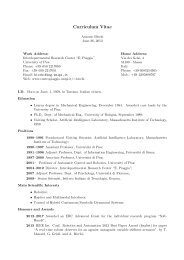
Stability and asymptotic stability 

606 Stabili 

Stability and attractivity of the origin 

Given a (closed-loop) system x + B✏(0) 

= f (x), with the 

origin as equilibrium, i.e. f (0) = 0 

The origin is locally stable if for every ɛ > 0, there 

x 

0 

exists δ > 0 such that |x| < δ implies |φ(k; x)| < ɛ 

The origin is globally attractive if 

lim k→∞ |φ(k; x)| = 0 for any x ∈ R n 

B (0) 

Global asymptotic stability and exponential stability 

Figure B.1: Stability of the origin. 

where A has eigenvalues 1 = 0.5 and 2 = 2 with associa 

vectors w1 and w2, shown in Figure B.2; w1 is the “stable” an 

“unstable” eigenvector; the smooth function (·) satisfies 

and (@/@x) (0) = 0 so that x + = Ax + (x) behaves like 

near the origin. If (x) ⌘ 0, the motion corresponding to 

state ↵w1, ↵ î 0, converges to the origin, whereas the mot 

sponding to an initial state ↵w2 diverges. If (·) is such tha 

nonzero states toward the horizontal axis, we get trajector 

|φ(k; x)| ≤ c|x|γ k formall shown k ≥in0 

Figure B.2. All trajectories converge to the o 

the motion corresponding to an initial state ↵w2, no matter h 

is similar to that shown in Figure B.2 and cannot satisfy the " 

tion of local stability. The origin is globally attractive but not 

G. Pannocchia <strong>Course</strong> on Model Predictive trajectory Control. Part that III – joins Stability anand equilibrium robustness point to itself, 4 / 36 as in Figu 

The origin is globally 

▶ 

▶ 

asymptotically stable (GAS) if it is locally stable and globally attractive 

exponentially stable (GES) if there exist c > 0 and γ ∈ (0,1) such that:

Asymptotic stability for constrained systems 

GAS for constrained system 

Let X be positively invariant for x + = f (x) 

The origin is 

▶ locally stable in X if for every ɛ > 0 there exists δ > 0 such that 

for any x ∈ X ∩ δB there holds |φ(k; x)| < ɛ for all k ≥ 0 

▶ attractive if for every x ∈ X there holds lim k→∞ |φ(k; x)| = 0 

▶ asymptotically stable in X if it is locally stable and attractive 

X is called region (or domain) of attraction for the origin 

Comparison function 

A function σ : R ≥0 → R ≥0 is of class K if it is continuous, σ(0) = 0 

and strictly increasing (K ∞ if unbounded) 

A function β : R ≥0 × N → R ≥0 is of class K L if for each t ∈ N, 

β(·, t) is a K function, and for each s ∈ R ≥0 , lim t→∞ β(s, t) = 0 

GAS is equivalent to |φ(k; x)| ≤ β(|x|,k) for all k ≥ 0, β(·) ∈ K L 


Lyapunov functions and asymptotic stability 

General definition 

A function V : R n → R ≥0 is a Lyapunov function for x + = f (x) 

if there exist K ∞ functions α 1 ,α 2 ,α 3 such that for all x ∈ R n : 

α 1 (|x|) ≤ V (x) ≤ α 2 (|x|) 

V (f (x)) −V (x) ≤ −α 3 (|x|) 

V decreases during the evolution of the system 

Lyapunov functions and GAS 

If V (·) is a Lyapunov function for x + = f (x), the origin is globally asymptotically 

stable 


Lyapunov functions and stability for constrained systems 

Asymptotic stability 

Then, the origin is asymptotically stable in X if: 

X is positively invariant for x + = f (x) 

V (·) is a Lyapunov function for x + = f (x) 

Exponential Lyapunov function and stability 

The origin of x + = f (x) is exponentially stable in X if 

X is positively invariant for x + = f (x) 

There exist V : R n → R ≥0 and positive constants a, a 1 , a 2 , a 3 : 

a 1 |x| a ≤ V (x) ≤ a 2 |x| a 

V (f (x)) −V (x) ≤ −a 3 |x| a 


Linear quadratic MPC formulation 

Prototype MPC problem 

Given current state x(0) = x, solve for the input sequence 

u = {u(0; x),u(1; x),...,u(N − 1; x)} 

Cost function: 

P N (x) : 

min u 

V N (x, u) s.t. 

x + = Ax + Bu 

x(j ) ∈ X for all j = 0,..., N − 1 

u(j ) ∈ U for all j = 0,..., N − 1 

x(N ) ∈ X f 

N−1 ∑ 

V N (x, u) = l(x(j ),u(j ))+V f (x(N )), 

j =0 

l(x,u) = x ′ Qx+u ′ Ru 

Terminal cost: V f (x) = x ′ P x 


Closed-loop system and basic path for stability 

Closed-loop system 

Given the optimal solution sequence u 0 (x), function of 

current state x, denote the implicit MPC control law 

κ N (x) = u 0 (0; x) 

Closed-loop system: x + = Ax + Bκ N (x) 

Notice that κ N : X N → U is not linear 

Basic route to prove stability 

Show that V 0 N 

(·) is a Lyapunov function for 

x + = f (x) = Ax + κ N (x) 

Show that the feasibility set, X N , is positively invariant 

(Control invariance of X f ) For every x ∈ X f , there exists 

u ∈ U: x + = Ax + Bu ∈ X f V f (x + ) −V f (x) ≤ −l(x,u) 


Stability proof 

Lemma. Optimal cost decrease 

For all x ∈ X N , there holds: V 0 N (Ax + Bκ N (x)) −V 0 N (x) ≤ −l(x,κ N (x)) 

Proof 

Consider the optimal input and state sequences 

u 0 (x) = {u 0 (0; x),u 0 (1; x),...,u 0 (N − 1; x)} 

x 0 (x) = {x 0 (0), x 0 (1),..., x 0 (N )} 

At next time, given x + = Ax + Bκ N (x), consider a candidate 

sequence ũ := {u 0 (1; x),...,u 0 (N − 1; x),u(N )} 

Choose u(N ) ∈ U such that x(N + 1) = Ax 0 (N ; x) + Bu(N ) ∈ X f 

and V f (x(N + 1)) + l(x(N ),u(N )) ≤ V f (x 0 (N )) 

ũ is feasible and V N (x + , ũ) ≤ V 0 N (x) − l(x,κ N (x)) 

But not optimal for P N (x + ). Thus: 

V 0 N (x+ ) ≤ V N (x + , ũ) ≤ V 0 N (x) − l(x,κ N (x)) 


Examples of linear MPC: the origin as terminal set 

Simple idea 

(No) Terminal cost: V f (x) = 0 

Terminal set: X f = {0} 

Drawbacks 

The feasibility set X N may be small because one needs to 

reach the origin in N steps (with constrained input u ∈ U) 

Closed-loop evolution of x + = Ax + Bκ N (x) and open-loop 

trajectory {x 0 (0), x 0 (1),..., x 0 (N − 1),0} may be very different 


Examples of linear MPC: Rawlings and Muske [1993] 

Open-loop stable systems 

Terminal cost: V f (x) := x ′ P x with P solution to the 

Lyapunov equation: 

∞∑ 

P = A ′ PA +Q notice that: P = (A j ) ′ Q A j 

Terminal set X f = X 

j =0 

Open-loop unstable systems 

][ 

Perform Schur decomposition: A = 

As A 

[ S s S u ][ 

su S ′ 

] 

s 

0 A u S u 

′ 

Solve reduced Lyapunov equation: Π = A ′ s ΠA s + S ′ s QS s 

Terminal cost: V f (x) = x ′ P x with P = S ′ s ΠS s 

Terminal set: X f = {x ∈ X | S ′ u x = 0} 


Examples of linear MPC: Scokaert and Rawlings [1998] 

Now considered the “standard” formulation 

Terminal cost: V f (x) = x ′ P x, from the Riccati equation: 

P = Q + A ′ PA − A ′ PB(B ′ PB + R) −1 B ′ PA 

Terminal set: X f = {x ∈ R n | V f (x) ≤ α} with α > 0 suitably 

chosen such that 

x ∈ X K x ∈ U with K = −(B ′ PB + R) −1 B ′ PA 

Comments 

Closed-loop and open-loop trajectories coincide 

It is an infinite-horizon optimal formulation 

Often the terminal constraint is not enforced, but verified 

a-posteriori (increasing N if not satisfied) 


Types of uncertainties 

... The bare truth 

The true controlled system does not satisfy x + = Ax + Bu 

The true state x is not known exactly 

Additive uncertainty 

The true system is modeled as 

x + = f (x,u) + w 

with f (x,u) = Ax + Bu 

The disturbance w is unknown but bounded, w ∈ W 

(W compact and convex) 

Alternative LTV description (convex hull) 

M∑ 

x(k + 1) = A(k)x(k) + B(k)u(k) with {A(k),B(k)} = µ i (k){A(i ),B(i )} 

i=1 


Closed-loop uncertain system under nominal MPC 

Difference inclusion description 

The true system can be modeled as a difference inclusion 

x + ∈ F (x,u) = {f (x,u) + w | w ∈ W} 

If the state is not precisely known: 

u = κ N (x + e) with e ∈ E (compact and convex) 

The closed-loop system evolves as: 

x + ∈ H(x) = {f (x,κ N (x + e)) + w | e ∈ E, w ∈ W} 

with a generic solution denoted as φ ew (k; x) 

Fundamental questions: if W and E are small sets 

Is P N solvable at all times (recursive feasibility)? 

Does the following robust stability condition hold? 

|φ ew (k; x)| ≤ β(|x|,k) + ɛ with ɛ > 0 


Inherent robustness of linear MPC 

Properties of P N for linear MPC [Grimm et al., 2004] 

The optimal cost function V 0 N 

(·) is continuous (in x) 

The optimal MPC law κ N (·) is continuous (in x) 

Robust asymptotic stability 

Grimm et al. [2004] showed that if: 

▶ 

▶ 

there exists a continuous Lyapunov function for the nominal 

system x + = f (x,κ N (x)), and 

P N is feasible at all times 

Then, for any ɛ > 0 there exists δ > 0 such that if {W,E} ∈ δB: 

|φ ew (k; x)| ≤ β(|x|,k) + ɛ 

In [Grimm et al., 2004] recursive feasibility was assumed 

... Proved in [Pannocchia et al., 2011a,b] 


What is suboptimal MPC? 

Why suboptimal MPC? ...A practical problem 

Despite its convexity (only for linear MPC), solving P N (x) up 

to optimality may be difficult if a short decision time is 

allowed 

Stability theory assumed that P N (x) is solved exactly 

What is the impact of using a suboptimal solution to P N (x)? 

A neat suboptimal MPC framework [Scokaert et al., 1999] 

Given current state x, previous control sequence 

u − = {u − (0),u − (1),...,u − (N − 1)} and state sequence 

x − = {x − (0), x − (1),..., x − (N )} 

Build a warm-start: u 0 = {u − (1),...,u − (N − 1),κ f (x − (N ))} 

Perform some iterations to improve the warm start: 

V N (x, u) ≤ V N (x, u 0 ) 


Stability under suboptimal MPC 

An additional ingredient 

To prove GAS, an additional requirement is enforced 

V N (x, u) ≤ V f (x) if x ∈ r B ⊂ X f 

r > 0 can be arbitrarily small: additional constraint will not matter 

Sketch of stability proof. 

Consider the extended state: z = (x, u) 

The successor suboptimal input sequence u + is a function of 

the x + and of the warm-start. Hence u + = g (x, u) 

The extended state evolves as 

[ 

] 

x + 

= 

u + ] 

[ 

Ax+B[I 0]u 

g (x,u) 

V N (·) is a Lyapunov function for z + = h(z) 

or z + = h(z) 

Additional condition implies GAS in the non-extended state 


Inherent robustness of suboptimal MPC (1/2) 

Comments on the suboptimal cost and control 

The suboptimal control is not unique, i.e. κ N (x) is 

set-valued map 

The suboptimal cost function V N (·) is not continuous in x 

The proof of [Grimm et al., 2004] for inherent robustness 

does not hold for suboptimal MPC 

New results [Pannocchia et al., 2011a,b] 

Suboptimal MPC is inherently robust 

Recursive feasibility can be established 

Optimal and suboptimal MPC have the same (qualitative) 

stability properties 


Inherent robustness of suboptimal MPC (2/2) 

Sketch of robust stability proof. 

The perturbed extended system evolves as a difference 

inclusion 

z + = H(z) := {(x + , u + ) | x + = Ax + Bu(0; x + e) + w, u + ∈ G(z)} 

Show exponential stability in the extended state 

Prove that exist γ ∈ (0,1) and µ > 0 

V N (z + ) ≤ max{γV N (z),µ} 

V N (·) is continuous in z and implies robust stability in the 

extended state 

The additional condition implies robust stability in the 

non-extended state 


Robust MPC design: an introduction (1/2) 

An example [Rawlings and Mayne, 2009] 

(Nominal) system: x + = x + u, without constraints X = U = R 

MPC design: N = 3, l(x,u) = x 2 + u 2 , V f (x) = x 2 

Open-loop control vs feedback policies 

OL Given initial state x(0) = x, solve for u = [u(0), u(1), u(2)] ′ : 

u 0 (x) = [ −0.615x −0.231x −0.077x ] ′ 

FB Use dynamic programming to obtain a feedback policy: 

µ 0 = [ −0.615x(0) −0.6x(1) −0.5x(2) ] ′ 

Evolution in the presence of uncertainties 

Same nominal evolution is obtained 

Considering disturbances: x + = x + u + w, different trajectories are obtained 


i 

Robust i MPC design: an introduction (2/2) 

Trajectories in three cases 

Three disturbance sequences: 

“book” — 2008/11/3 — 17:21 — page 178 — #210 

▶ w 0 = {0, 0, 0} 

▶ w 1 178 

= {1, 1, 1} 

Robust Model Predictive Control 

▶ w 2 = {−1, −1, −1} 

2 

x1 

2 

x1 

X1 

X2 

X3 

X1 

X2 

X3 

x0 

x0 

0 

1 

2 

k 

3 

0 

1 

2 

k 

3 

x2 

x2 

2 

2 

(a) Open loop. 

(b) Feedback. 

Feedback policies Figure 3.1: are Open-loop clearly more and feedback effective trajectories. against disturbances 


Min-max MPC 

Conceptual framework 

Prediction model x + = Ax + Bu + w with w ∈ W (compact) 

Robustly invariant terminal set X f [Blanchini, 1999] 

Open-loop min-max: u = [ u(0) u(1) ··· u(N−1)] 

min u 

max 

w V N (x, u, w) s.t. 

x(j + 1) = Ax(j ) + Bu(j ) + w(j ) 

x(j ) ∈ X, w(j ) ∈ W, u(j ) ∈ U for j = 0,..., N − 1 

x(N ) ∈ X f 

Feedback min-max: µ = [ µ(x(0)) µ(x(1)) ··· µ(x(N−1))] 

min max V N (x,µ, w) s.t. 

µ w 

x(j + 1) = Ax(j ) + Bµ(x(j )) + w(j ) 

x(j ) ∈ X, w(j ) ∈ W, µ(x(j )) ∈ U for j = 0,..., N − 1 

x(N ) ∈ X f 


Tube-based MPC (1/3) 

Set algebra 

Some notation 

▶ Set addition: A ⊕ B = {a + b | a ∈ A, b ∈ B} 

▶ Set subtraction: A ⊖ B = {x ∈ R n | {x} ⊕ B ⊆ A} 

▶ Set multiplication: let K ∈ R m×n . K A = {K a | a ∈ A} 

Outer-bounding tube 

Uncertain linear system: x + = Ax + Bu + w, w ∈ W 

Nominal system: z + = Az + Bv 

Affine feedback policy: u = v + K (x − z) 

Error, e = x − z, evolves as: e + = (A + BK )e + w = A K e + w 

If we set z(0) = x(0), i.e. e(0) = 0, then 

i−1 ∑ 

e(i ) ∈ S K (i ) = A j K W ⊆ S 

j =0 



Constraint tightening 

Constraints on the uncertain system: x(i ) ∈ X, u(i ) ∈ U 

i 

Tightened constraints on the nominal system: 

z(i ) ∈ Z = X ⊖ S, v(i ) ∈ V = U ⊖ K S 

i 

“book” — 2008/11/3 — 17:21 — page 212 — #244 

A sketch of nominal and uncertain trajectories 

212 Robust Model Predictive Control 

i 

i 

X1 

x2 

x trajectory 

X0 

X2 

z trajectory 

x1 

S0 

Figure 3.4: Outer-bounding tube X(z, v). 



Nominal MPC problem with restricted constraints 

¯P N (z) : 

min v 

V N (z, v) s.t. z + = Az + Bv 

z(j ) ∈ Z for all j = 0,..., N − 1 

v(j ) ∈ V for all j = 0,..., N − 1 

z(N ) ∈ Z f 

Tube-based MPC 

Initialization At time k = 0, set z(0) = x(0) 

Step 1 Given current augmented state (x, z), solve ¯P N (z) and obtain 

nominal control v = ¯κ N (z) 

Step 2 Apply control: u = v + K (x − z) 

Step 3 Compute nominal successor state: z + = Az + Bv and measure 

successor state x + 

Step 4 Replace (x, z) ← (x + , z + ), go to Step 1 


Output feedback MPC: main definitions 

True system and state estimator 

Uncertain LTI system 

x + = Ax + Bu + w 

y = C x + v 

Bounded disturbances: w ∈ W, v ∈ V 

Simple Luenberger observer: 

ˆx + = A ˆx + Bu + L(y − ŷ) 

Estimation error e := x − ˆx evolves as 

with ŷ = C ˆx 

e + = (A − LC )e + ˜w 

with ˜w := w − Lv ∈ ˜W := W ⊕ (−LV) 

Output feedback MPC 

Solve P N ( ˆx) and apply κ N ( ˆx) 


Nominal stability of output feedback MPC 

Deterministic case 

In the ideal situation: W = {0} and V = {0}: e + = (A − LC )e 

The origin of e + = (A − LC )e is exponentially stable 

Estimator state evolves as: ˆx + = A ˆx + Bu + LCe 

Main result [Scokaert et al., 1997] 

Let φ(k; x,e) be the solution at time k of x + = Ax + Bκ N ( ˆx) 

The following asymptotic stability condition holds: 

|φ(k; x,e)| ≤ β(|(x,e)|,k) for all k ∈ N 

for any initial state x ∈ C ⊂ X N and estimate error e ∈ E 


Offset-free MPC based on disturbance model 

Some reminders 

The augmented system (x ∈ R n ,u ∈ R m , y ∈ R p ,d ∈ R n d ) 

x + = Ax + Bu + B d d 

d + = d 

y = C x +C d d 

Observability requirements 

(A,C ) observable rank[ 

A−I Bd 

C C d 

] 

= n + n d 

Tracked variables, target calculator and dynamic optimization 

Controlled variables: r = H y, with r ∈ R p r 

and p r ≤ min{p,m} 

Target calculator chooses targets (x s ,u s ) such that: 

x s = Ax s + Bu s + B d d, ¯r = H(C x s +C d d) 

Dynamic optimization regulates deviation variables: 

˜x = x − x s → 0, ũ = u − u s → 0 


Zero offset [Muske and Badgwell, 2002, Pannocchia and 

Rawlings, 2003, Maeder et al., 2009] 

Theorem statement 

Let n d = p, assume that: 

▶ 

▶ 

MPC feasible at all times, unconstrained for k ≥ ¯k 

Closed loop reaches steady values: (u ∞ , y ∞ ), ( ˆx ∞ , d ˆ ∞ ), (x s ,u s ) 

Then, there is zero offset in r : r ∞ = H y ∞ = ¯r 

Sketch of proof 

Stability of the observer implies that L d ∈ R p×p is full rank: 

dˆ 

∞ = d ˆ ∞ + L d (y ∞ −C ˆx ∞ −C d d∞ ˆ ) ⇒ y ∞ = C ˆx ∞ +C d d∞ ˆ 

Target satisfies: ¯r = H(C x s +C d d∞ ˆ ) 

Since constraints are inactive (at steady state), ũ ∞ = K ˜x ∞ 

Hence: ˜x ∞ = (A + BK ) ˜x ∞ ⇒ ˜x ∞ = ˆx ∞ − x s = 0 ⇒ ˆx ∞ = x s 

Combining all steps: H(C ˆx ∞ +C d ˆ d∞ ) = H y ∞ = r ∞ = ¯r 


Equivalence of disturbance models and observer design 

A debate: what is the best choice for (B d ,C d )? 

There were evidences that B d = 0, C d = I was a bad choice 

[Lundström et al., 1995, Muske and Badgwell, 2002, 

Pannocchia, 2003, Pannocchia and Rawlings, 2003, Maeder 

et al., 2009, Bageshwar and Borrelli, 2009] 

A change of perspective 

Rajamani et al. [2004, 2009] argued that two augmented 

systems with same (A,B,C ) and different (B d ,C d ) are two 

non-minimal realizations of the same system 

A transformation matrix T makes them equivalent 

A 1 = [ ] 

A B d1 

0 I , B1 = [ ] [ ] 

B Lx1 

0 

, C1 = [C C d1 ], L 1 = 

L d1 

A 2 = [ ] 

A B d2 

0 I = T A1 T −1 , B 2 = [ ] 

B 

0 

= T B1 , C 2 = [C C d1 ] = 

C 1 T −1 , L 2 = T L 1 

Choose any (B d ,C d ) and determine (L x ,L d ) from data 


H ∞ interpretation of disturbance models 

H ∞ interpretation [Pannocchia and Bemporad, 2007] 

System P subject to a disturbance w ∈ R n+p 

x + = Ax + Bu + B w w B w = [ I n 0] 

y = C x + +D w w D w = [ 0 I p ] 

Design a dynamic observer L : 

ξ + = A L ξ + B L e 

with e = y − ŷ 

v = C L ξ + D L e 

Estimator in closed loop: 

ˆx + = A ˆx + Bu + B v v B v = [ I n 0] 

ŷ = C x + +D v v D v = [ 0 I p ] 

Equivalent to the augmented system and observer: 

A L = I p , B d = AB v C L , C d = D v C L 

L x = AB v D L (I + D v D L ) −1 , L d = B L (I + D v D L ) −1 

An H ∞ observer L such that the DC-gain w → s = e 

is zero is such that A L = I 

s 

e 

P 

L 

w 

v 


Alternative methods for offset-free MPC design (1/2) 

Delta input form 

Assume for simplicity r = y. Define δu(k) = u(k) − u(k − 1), 

i.e. u(k) = u(k − 1) + δu(k), and the augmented system 

] 

= [ ] 

A B 

+ [ ] 

B 

I 

δu(k) 

[ 

x(k+1) 

u(k) 

y(k) = [C 0] 

Observer to estimate x a (k) = 

0 I m 

] [ x(k) 

u(k−1) 

[ ] 

x(k) 

u(k−1) 

[ 

x(k) 

u(k−1) 

Solve the dynamic optimization penalizing (y − ¯r ) and δu 

Apply u(k) = u(k − 1) + δu 0 (k) 

] 

Observations 

The system is observable only if p ≥ m 

Does not require a target calculator 

True input u(k − 1) and its estimate û(k − 1) may be different 


Alternative methods for offset-free MPC design (2/2) 

Velocity form 

δx(k) = x(k) − x(k − 1), δu(k) = u(k) − u(k − 1), z = y − ¯r 

Augmented system: 

[ ] [ ] 

δx + A 0 

[ ] [ 

z 

= 

δx 

C A I p z + B 

] 

CB 

δu 

y − ¯r = [ 0 I ] [ ] 

δx 

z 

Observer to estimate x a = [ ] 

δx 

z 

Solve the dynamic optimization penalizing z and δu 

Apply u(k) = u(k − 1) + δu 0 (k) 

Observations 

The system is stabilizable only if p ≤ m 

Does not require a target calculator 

May show windup issues if the setpoint ¯r is not reachable 


References I 

V. L. Bageshwar and F. Borrelli. On a property of a class of offset-free model predictive controllers. IEEE 

Trans. Auto. Contr., 54(3):663–669, 2009. 

F. Blanchini. Set invariance in control. Automatica, 35:1747–1767, 1999. 

G. Grimm, M. J. Messina, S. E. Tuna, and A. R. Teel. Examples when nonlinear model predictive control 

is nonrobust. Automatica, 40:1729–1738, 2004. 

P. Lundström, J. H. Lee, M. Morari, and S. Skogestad. Limitations of dynamic matrix control. Comp. 

Chem. Eng., 19:409–421, 1995. 

U. Maeder, F. Borrelli, and M. Morari. Linear offset-free model predictive control. Automatica, 45(10): 

2214–2222, 2009. 

K. R. Muske and T. A. Badgwell. Disturbance modeling for offset-free linear model predictive control. J. 

Proc. Contr., 12:617–632, 2002. 

G. Pannocchia. Robust disturbance modeling for model predictive control with application to 

multivariable ill-conditioned processes. J. Proc. Cont., 13:693–701, 2003. 

G. Pannocchia and A. Bemporad. Combined design of disturbance model and observer for offset-free 

model predictive control. IEEE Trans. Auto. Contr., 52(6):1048–1053, 2007. 

G. Pannocchia and J. B. Rawlings. Disturbance models for offset-free model predictive control. AIChE J., 

49:426–437, 2003. 

G. Pannocchia, J. B. Rawlings, and S. J. Wright. Conditions under which suboptimal nonlinear MPC is 

inherently robust. Syst. Contr. Lett., 60:747–755, 2011a. 


References II 

G. Pannocchia, S. J. Wright, and J. B. Rawlings. Partial enumeration MPC: Robust stability results and 

application to an unstable cstr. J. Proc. Contr., 21(10):1459–1466, 2011b. 

M. R. Rajamani, J. B. Rawlings, and J. Qin. Optimal estimation in presence of incorrect disturbance 

model. Technical Report 2004–09 (Draft), TWMCC, Department of Chemical Engineering, University 

of Wisconsin-Madison, March 2004. 

M. R. Rajamani, J. B. Rawlings, and S. J. Qin. Achieving state estimation equivalence for misassigned 

disturbances in offset-free model predictive control. AIChE J., 55(2):396–407, 2009. 

J. B. Rawlings and D. Q. Mayne. Model Predictive Control: Theory and Design. Nob Hill Publishing, 

Madison, WI, 2009. 

J. B. Rawlings and K. R. Muske. Stability of constrained receding horizon control. IEEE Trans. Auto. 

Contr., 38:1512–1516, 1993. 

P. O. M. Scokaert and J. B. Rawlings. Constrained linear quadratic regulation. IEEE Trans. Auto. Contr., 

43:1163–1169, 1998. 

P. O. M. Scokaert, J. B. Rawlings, and E. S. Meadows. Discrete-time stability with perturbations: 

Application to model predictive control. Automatica, 33:463–470, 1997. 

P. O. M. Scokaert, D. Q. Mayne, and J. B. Rawlings. Suboptimal model predictive control (feasibility 

implies stability). IEEE Trans. Auto. Contr., 44:648–654, 1999.

Course on Model Predictive Control Part III ... - Centro E Piaggio

You also want an ePaper? Increase the reach of your titles

Delete template?

Save as template?