Trajectory Control of a Four-Wheel Skid-Steering Vehicle Over Soft ...

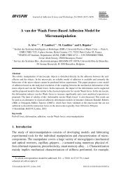
2007 IEEE International Conference on
Robotics and Automation
Roma, Italy, 10-14 April 2007
WeD5.2
Trajectory Control of a Four-Wheel Skid-Steering Vehicle over Soft
Terrain using a Physical Interaction Model
D. Lhomme-Desages ∗ ,Ch.Grand ∗ and J-C. Guinot ∗
∗ Laboratoire de Robotique de Paris
Route du Panorama, 92260 Fontenay-aux-Roses
lhomme@robot.jussieu.fr, grand@robot.jussieu.fr, guinot@robot.jussieu.fr
Abstract— A model-based control for fast autonomous fourwheel
mobile robots on soft soils is developed. This control
strategy takes into account slip and skid effects to extend the
mobility over planar granular soils. Each wheel is independently
actuated by an electric motor. The overall objective is to follow
a path roughly at relatively high speed. Some results obtained
in dynamic simulation are presented.
I. INTRODUCTION
Many popular controllers for wheeled mobile robots assume
that wheels roll without slipping. This leads to a
nonholonomic constraint added to the kinematic or dynamic
model [1]. This assumption is quite legitimate for usual
applications such as autonomous cars over hard terrains or
slow indoor exploration. However, it is no longer suitable for
many applications where wheel slip cannot be neglected [2],
especially for traveling over natural soils at high speed [3].
With this type of control architecture, the stability of the
rover cannot be guaranteed in presence of slippage, due to
the dynamics of the vehicle and the saturation of admissible
forces by the soil. Therefore, a new control scheme is
required.
In this paper, a model-based control method for fast
autonomous mobile robots on soft soils is developed. On
such a type of terrain (sand for instance), slip and skid
phenomena may be significant. The control strategy takes
into account these effects to extend the mobility of the
vehicles over natural soils. The terrains considered here are
horizontal and relatively smooth compared to the size of the
wheels.
A non-linear model-based control of wheel slippage is
studied, using a semi-empirical wheel-soil interaction model.
A higher-level control is applied to a four-wheel skid-steering
vehicle which can travel at relatively high speed (several
meters per second). Each wheel is independently actuated
by an electric motor.
The overall objective is to follow a given trajectory at
relatively high speed. This controller implies a low-level
control method that aims to regulate the slip rate of one
wheel, since the traction force generated by the rotation of
the wheel at the contact patch depends on the wheel slip.
Limitations and required sensors are also pointed out.
Finally, this control scheme is evaluated in dynamic simulation.
The results show an improvement of motion control
when implementing the model-based traction control.
II. SYSTEM MODELLING
A. Rover model
We consider a skid-steering vehicle with four independent
electrically driven wheels. The kinematic and geometric
parameters of the vehicle are shown on figure 1.
X
M ψ
O3
Y
ψ
F Y
b F X
a
O4
G
O2
v
Γ
y
F l1 F
ω
t1
R
O1
F t
x
z X
O
Fig. 1.
Model of a four-wheel rover
The center of mass G is located at the center of the
platform. See Tab. I for a description of notations. ψ is the
orientation of the vehicle relatively to (O, x).
B. Wheel-soil interaction model
Several modeling frameworks can be used to calculate the
forces involved in the wheel-soil interaction process. We use
an extended version of the terramechanic model introduced
by Bekker ([4],[5]). We assume that the entire wheel is very
stiff compared to the ground and we can consider that the
wheel is rigid (Fig. 2).
D
R
F n
ω
R
θ θ 1
z
R r
z
F t
w w l
Fig. 2.
Model of a rigid wheel
v
1-4244-0602-1/07/$20.00 ©2007 IEEE. 1164

WeD5.2
Denote v the velocity of the center of the wheel, and ω
the angular velocity of the wheel. In this model, the traction
force depends on the slip rate s, which is defined as:
{ 1 −
v
s =
ω.R
if Rω ≥ v
1 − ω.R
(1)
v
if Rω < v
for v>0 and ω>0. This definition can be extended to
every (v, ω) ∈R 2 , as is shown in Fig. 3.
F tmax
F t (N)
−F tmax
19
16
13
10
7
4
1
0
s
z =5mm
F n =44.2 N
8 6 4 2 0 0.2 0.4 0.6 0.8 1
Fig. 4.
Traction force vs. slip rate
Fig. 3.
Slip rate as a function of v and Rω
F l = μ l (d l ).F n = μ ls
(
1 − e d l/d ls
)
F n (6)
where d ls and μ ls are soil characteristics, d l is the lateral
displacement.
This contact model has been validated by experimental
measurements on an instrumented testing bench (Fig. 5).
A set of experimental data is depicted in Fig. 6. A curvefitting
algorithm is used to find the soil parameters of the
interaction model. The resulting curve fits relatively well the
data, despite a high experimental noise of about ±10 N.
According to Bekker theory [4], the normal force depends
on the wheel sinkage z through:
F n = 1 [ ( )
kc
w w
3 r + k φ (3 − n) √ ]
Dz 2n+1
2 (2)
where k c , k φ and n are soil parameters. w w is the width of
the wheel.
r = min(w w ,l), l being the length of the contact patch.
The net traction force DP (also known as drawbar pull) is
the difference between the raw traction force and the rolling
resistance:
Fig. 5.
Experimental device
DP(s) =F t (s) − R r (3)
In this study, the rolling resistance is assumed to be
mainly caused by soil compaction, which allows to use the
expression:
z n+1 ( )
kc
R r = w w
n +1 r + k φ
(4)
The raw traction force is related to the slip rate:
[ (
F t (s) =F )]
m 1 −
K
s.l 1 − e
−s.l/K
(5)
F m = lw w c + F n tan φ
where c, φ and K are soil cohesion, friction angle and shear
deformation modulus, respectively.
The shape of F t is plotted on Fig. 4 with parameters of
Tab. I. This is a monotonic function and it reaches its extreme
values ±F tmax for extreme values of s.
Lateral forces can be implemented, including bulldozing
resistance, as described in [6]. In this study, we use a simple
linearized Coulomb model for lateral forces:
III. TRAJECTORY TRACKING CONTROL
The objective of this model-based control scheme is the
tracking of a reference trajectory given under the form
(x ∗ (t),y ∗ (t),ψ ∗ (t)).
We denote F the global vector of forces and torque applied
to the center of mass of the platform, in the local frame
attached to the chassis. This vector has two components
since the lateral motion is uncontrollable: no combination
of traction forces can result in a lateral motion. Therefore,
the lateral component F Y is ignored:
[ ]
FX
F =
(7)
M ψ
A. Control architecture
Figure 7 presents the overall control system. The role of
the trajectory controller is to generate a proper desired global
force F ∗ . Then each raw traction force F ∗
t is computed
from the global desired force by solving the forces balance.
Lateral forces and rolling resistance are estimated using the
1165

WeD5.2
( x ∗ , y ∗ , ψ ∗ )
y
x
M ψ
∗
v ∗
d
ψ ∗˜ψ
G
F X
∗
ψ
Fig. 8.
Parameters for the trajectory control
Fig. 6.
Experimental measure of drawbar pull
terramechanic model. The inversion of the estimated wheelsoil
contact model provides the desired slip rate s ∗ from F t ∗ .
X ∗
Ẋ ∗
Dynamic
Trajectory
Controller
F ∗ +
∗
A t
F t
F
ˆF l
lateral forces
estimator
Fig. 7.
s
s ∗
X
Traction
Controller
slip
computer
Ẋ
s
Control block diagram
This architecture is composed of two stages, the trajectory
control and the traction control, which are detailed in the
next sections. The traction controller regulates the slip rate
of each wheel.
The input desired torques are saturated to ensure that
desired values do not exceed actuators capabilites.
B. Trajectory controller
The trajectory controller is a high-level module that
generates a desired F ∗ corresponding to a desired motion
of the robot toward the desired trajectory (Fig. 8). The
desired global force depends on the kinematic and geometric
situation (F ∗ = f(X, Ẋ)).
Note d the distance between the platform center of mass
and the desired reference position.
Define the errors in velocity and heading angle:
Γ
Rover
e v = v ∗ − v (8)
e ψ = ˜ψ − ψ (9)
Instead of the reference angle ψ ∗ (t) of the reference
trajectory, the desired angle is:
ω
˜ψ(d) =ψ ∗ − arctan(k f d) (10)
This defines a modified reference angle that depends also
on the distance d. k f is a tuning parameter. Equation (10)
is intended to reduce the distance to the reference trajectory
even with a passive lateral motion.
A simple strategy may be defined as the following:
F X ∗ = k pX e v + k iX
∫
e v (11)
M ψ ∗ = k pψ e ψ + k iψ
∫
e ψ + k dψ e˙
ψ (12)
where k iX , k pX , k pψ , k iψ and k dψ are gains. This defines a
PI-controller on operational velocity v and a PID-control of
the heading angle ψ.
C. Tractive force distribution
Each wheel is subjected to tangential lateral and longitudinal
contact forces, gathered in corresponding vectors:
F t =[DP 1 ,DP 2 ,DP 3 ,DP 4 ] T (13)
F l =[F l1 ,F l2 ,F l3 ,F l4 ] T (14)
The position of the robot is the position of the platform
center of mass in the referential frame:
X =[x, y, ψ] T (15)
and ω is the vector of angular velocities of the wheels.
For each wheel, we can separate the contributions of lateral
and longitudinal forces, which are related to the global force
by a linear equation:
) )
F = A t F t
(Ẋ, ω + A l F l
(Ẋ (16)
with:
A t =
[
1 1 1 1
b b −b −b
]
(17)
1166

WeD5.2
A l =
[
0 0 0 0
−a a a −a
]
(18)
Therefore, assuming translation and angular velocities are
known, we can deduce the longitudinal forces to apply. Angular
velocities can be easily measured via optical encoders.
Ground velocity can be estimated using a Doppler sensor for
instance [7].
We can inverse the linear system (16) by minimizing the 2-
norm of vector Ft (thus minimizing tractive efforts). Using
the pseudo-inverse of A t , the optimal tractive efforts are
computed from equation (19), where hats denote estimated
values, and stars denote desired values:
( )
F ∗ +
t = A t F ∗ − A l̂Fl (19)
The pseudo-inverse of this matrix A t can be symbolically
solved:
⎡ ⎤
b 1
A + t = 1 ⎢ b 1 ⎥
⎣
4b b −1 ⎦ (20)
b −1
D. Model-based traction control
In order to apply motor torques corresponding to desired
traction efforts, the interaction contact model is used to take
into account the capabilities of the ground.
The forces balance equation gives the desired net traction
force DP for each wheel. Using the Bekker-Wong model
described in section II, the rolling resistance is first estimated
from eq. (4). To perform this estimation, an estimation of the
sinkage z is calculated on the basis of eq. (2). Normal forces
F ni are assumed to be equal to the fourth of the total weight:
F ni =(m c +4m r )g/4, 1 ≤ i ≤ 4 (21)
This strong assumption means that the center of mass is
located at the center of the platform and that there is no
lateral or longitudinal load transfers.
Then, the raw traction force F t is computed using eq. (3).
Finally, the F t (s) function (eq. (5)) can be inversed to obtain
a desired slip rate.
The tractive efforts can be unreachable if we consider the
contact model. If the desired force is not admissible by the
soil (|F t | > F tmax , i.e. |s| = 1), then the robot will be
unable to follow the path with accuracy and will skid.
The lateral efforts ̂F l are estimated with the lateral contact
model and a measure of the kinematic state of the vehicle.
E. Slip servoing
Several slip control methods exist in the literature, including
nonlinear and gain-scheduled PID, sliding mode [8],
fuzzy logic [9], or Lyapunov synthesis [10].
Simple slip control strategies have been used for several
mobile robots in rough terrain ([11], [12]). Like these
authors, we implement a simple PI-controller (Fig. 9). A
derivative gain is inappropriate since the slip rate is a
s ∗
+
-
Fig. 9.
s
1
s
K i
K p
slip
+
+
Γ
Motor
Control block diagram with PI-controller
discontinuous function. Each independent electric motor is
controlled in torque (namely in current).
Numerical simulations of a one-wheel vehicle have been
led in a dynamical multibody modeling software [13]. An
extension to this software has been developed to implement
the terramechanic contact model. The step response of the
controller is depicted on Fig. 10 (s ∗ =0.8, K p = K i = 100).
1.0
0.8
0.75
0.5
0.25
0.0
0.0
s
s ∗
0.5
time (seconds)
Fig. 10. Comparison between step desired and simulated slip rate with
PI-control
After a short period where s is not continuous (at t =0 + ,
v =0and ω>0, see Fig. 3), it converges toward the desired
value.
IV. SIMULATION RESULTS
To simulate the behavior of the robot, a simple desired
maneuver has been chosen, which is a right bend at constant
desired tangential velocity (1.7 m/s) after an acceleration
phase at constant rate. The minimal radius of curvature is 54
cm. Kinematic, dynamical and contact parameters are given
in the table I. Soil parameters correspond to a dry sandy
soil [5]. Dynamic and geometrical parameters are those of a
project of a testing skid-steering platform.
A passive revolute joint has been introduced between both
sides of the platform to guarantee an isostatic contact.
A. Trajectory control without traction control
In order to test and validate the traction control, a simulation
is made without the model-based traction control
subsystem. Therefore, the contact model is not involved in
the control architecture and the lateral forces are ignored,
which means they are processed as perturbations. Since the
contact model is not used, the rolling resistance is also
ignored, so it is implicitly assumed that F t = DP for each
wheel.
In this case, the distribution of the global desired force is:
1.0
1.5
2.0
1167

WeD5.2
TABLE I
SIMULATION PARAMETERS
m r 1 kg wheel mass
m c 14 kg chassis mass
J 1.03.10 −2 kg.m 2 wheel inertia
R 10 cm wheel radius
w w 6 cm wheel width
a 35 cm half wheelbase
b 23 cm half track width
n 0.705 soil exponent
k c 6940 N.m −(n+1) cohesive modulus
k φ 505800 N.m −(n+2) friction modulus
φ 31.5 deg friction angle
c 1150 Pa cohesion
K 1.15 cm soil modulus
K p 300 proportional gain for slip servoing
K i 1000 integral gain for slip servoing
rad
1.57
0.3925
0.0
-0.785
-1.9625
-3.14
0.0
Fig. 13.
1.0 2.0
3.0
ψ
˜ψ
4.0
time (seconds)
ψ ∗
5.0 6.0 7.0
Rover direction and desired heading angle
1.5
F t ∗ = A t + F ∗ (22)
1.5
v ∗
For each wheel, the desired traction force Ft
∗
translated to a torque using:
is directly
m/s
0.5
v
Γ=RF t
∗
(23)
The inertial term of the dynamic equation of the wheel
motion is ignored, as well as the soil capabilities. The
resulting control architecture is represented on Fig. 11.
0.0
-0.5
0.0
1.0
2.0
3.0
4.0
time (seconds)
5.0
6.0
7.0
X
Fig. 14.
Rover velocity
X ∗
Ẋ ∗
Dynamic
Trajectory
Controller
F ∗
A t
+
F t
∗
1/R
Γ
Ẋ
Rover
It can be seen from Fig. 15 that the slip rate reaches its
maximum (soil failure regions). The ground cannot admit
traction forces that are required to stabilize the system.
Fig. 11.
Control block diagram
1.0
The simulation gives the sequence shown in Fig. 12.
10
0.5
0.0
s 1
s 3
y(m)
-0.5
-1.0
0.0
1.0
2.0
3.0 4.0
time (seconds)
soil failure
5.0
6.0
soil failure
7.0
Fig. 15.
Slip rates
1
0 1
x(m) 10
Fig. 12. Trace of the motion of the rover
The unstable behavior of the system is clearly highlighted.
For this particular set of parameters and gains, the system
is unstable. More generally, the control of this type of
autonomous robots in presence of large slip is problematic.
B. Model-based Trajectory control
With the implementation of the control architecture developed
in this paper, we obtain the sequence of the figure 16.
Despite the lack of accuracy of the tracking, which is sec-
1168

WeD5.2
d =1.2m
max
Fig. 19.
Skid-steering demonstrator
rad
1.0
0.5
0.0
-0.5
-1.0
-1.5
Fig. 16.
Trace of the motion of the rover
-2.0
-2.5
-3.0
-3.5
0.0
Fig. 17.
1.0
2.0
3.0
4.0
time (seconds)
ψ ∗˜ψ
V. CONCLUSION AND FUTURE WORKS
The controller presented in this paper may be useful to
achieve better performances on challenging terrains such as
planetary surfaces, but requires a larger instrumentation. In
particular, this model-based control may be used for obstacle
avoidance at high speed.
Further works are being made to implement this control
strategy in a fast mobile robotic platform under development
(Fig. 19). Absolute ground velocity will be measured with
a Doppler radar sensor. Robustness and sensitivity to soil
parameters have to be evaluated. If the algorithm is robust
enough, then a real-time nonlinear estimation of contact
parameters is not required as long as the terrain is relatively
homogeneous. An off-line initialization procedure may be
suitable.
m/s
2.0
1.5
1.0
0.5
0.0
-0.5
-1.0
0.0
1.0
Rover direction and desired heading angle
2.0
Fig. 18.
3.0
4.0
v
v ∗
time (seconds)
5.0
5.0
Rover velocity
ondary for high-speed applications, the control architecture
allows the stability of the system.
The figure 18 shows that the tangeantial velocity can be
negative, which is acceptable, but very inefficient for power
consumption.
These results show that the trajectory tracking is improved
under such conditions with the model-based control scheme
developed in section III .
ψ
6.0
6.0
7.0
7.0
8.0
8.0
REFERENCES
[1] L. Caracciolo, A. De Luca, and S. Iannitti, “Trajectory tracking control
of a four-wheel differentially driven mobile robot,” in Proc. IEEE Intl
Conf. on Robotics & Automation, Detroit, USA, May 1999, pp. 2632–
2638.
[2] T. Huntsberger, H. Aghazarian, Y. Cheng, E. Baumgartner, E. Tunstel,
C. Leger, A. Trebi-Ollennu, and P. S. Schenker, “Rover autonomy
for long range navigation and science data acquisition on planetary
surfaces,” in Proc. IEEE Intl Conf. on Robotics & Automation,
Washington DC, USA, May 2002, pp. 3161–3168.
[3] M. Spenko, K. Iagnemma, and S. Dubowsky, “High speed hazard
avoidance for mobile robots in rough terrain,” in SPIE Conf. on
Unmanned Ground Vehicles, 2004.
[4] M. Bekker, Introduction to Terrains-Vehicles Systems. The University
of Michigan Press, 1969.
[5] J. Y. Wong, Terramechanics and Off-Road Vehicles. Elsevier, 1989.
[6] G. Ishigami, A. Miwa, and K. Yoshida, “Steering trajectory analysis of
planetary exploration rovers based on all-wheel dynamics model,” in
8th Intl Symposium on Artifical Intelligence, Robotics and Automation
in Space, Munich, Germany, Sept. 2005.
[7] S. Stuchly, A. Thansandote, J. Mladek, and J. Townsend, “A doppler
radar velocity meter for agricultural tractors,” IEEE Trans. Veh.
Technol., vol. 27, no. 1, pp. 24–30, Feb. 1978.
[8] K. Buckholtz, “Reference input wheel slip tracking using sliding
mode control,” in SAE World Congress Detroit, Society of Automotive
Engineers. SAE, Mar. 2002.
[9] F. Yu, J.-Z. Feng, and J. Li, “A fuzzy logic controller design for vehicle
abs with a on-line optimized target wheel slip ratio,” Intl Journal of
Automotive Technology, vol. 3, no. 4, pp. 165–170, 2002.
[10] J. Kalkkuhl, T. Johansen, and J. Ludemann, “Improved transient performance
of nonlinear adaptive backstepping using estimator resetting
based on multiple models,” IEEE Trans. Automat. Contr., vol. 47, pp.
136–140, 2002.
[11] K. Yoshida and H. Hamano, “Motion dynamics of a rover with
slip-based traction model,” in Proc. IEEE Intl Conf. on Robotics &
Automation, Washington, DC, USA, May 2002, pp. 3155–3160.
[12] D. Caltabiano, D. Ciancitto, and G. Muscato, “Experimental results on
a traction control algorithm for mobile robots in volcano environment,”
in Proc. IEEE Intl Conf. on Robotics & Automation, New Orleans,
USA, Apr. 2004, pp. 4375–4380.
[13] Msc adams. [Online]. Available: www.mscsoftware.com/products
1169