Document Title - Geoscience Australia

G E O S C I E N C E A U S T R A L I A 

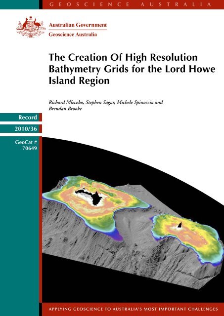
The Creation Of High Resolution 

Bathymetry Grids for the Lord Howe 

Island Region 

Record 

Richard Mleczko, Stephen Sagar, Michele Spinoccia and 

Brendan Brooke 

2010/36 

GeoCat # 

70649 

APPLYING GEOSCIENCE TO AUSTR ALIA’S MOST IMPORTANT CHALLENGES

The Creation of High Resolution 

Bathymetry Grids for the Lord Howe 

Island Region 

GEOSCIENCE AUSTRALIA 

RECORD 2010/36 

by 

Richard Mleczko, Stephen Sagar, Michele Spinoccia and Brendan Brooke.

Department of Resources, Energy and Tourism 

Minister for Resources and Energy: The Hon. Martin Ferguson, AM MP 

Secretary: Mr John Pierce 

Geoscience Australia 

Chief Executive Officer: Dr Chris Pigram 

© Commonwealth of Australia, 2010 

This work is copyright. Apart from any fair dealings for the purpose of study, research, criticism, 

or review, as permitted under the Copyright Act 1968, no part may be reproduced by any process 

without written permission. Copyright is the responsibility of the Chief Executive Officer, 

Geoscience Australia. Requests and enquiries should be directed to the Chief Executive Officer, 

Geoscience Australia, GPO Box 378 Canberra ACT 2601. 

Geoscience Australia has tried to make the information in this product as accurate as possible. 

However, it does not guarantee that the information is totally accurate or complete. Therefore, you 

should not solely rely on this information when making a commercial decision and the data 

contained herein is not to be used for navigation. 

Certain material reproduced under licence by permission of The Australian Hydrographic Service. 

© Commonwealth of Australia 2010. All rights reserved. This information may not be copied, 

reproduced, translated, or reduced to any electronic medium or machine readable form, in whole or 

part, without the prior written consent of the Australian Hydrographic Service. 

ISSN 1448-2177 

ISBN 978-1-921781-39-1 (Print) 

ISBN 978-1-921781-40-7 (Web) 

GeoCat # 70649 

Bibliographic reference: Mleczko, R., Sagar, S., Spinoccia, M., and Brooke, B. 2010. The Creation 

of High Resolution Bathymetry Grids for the Lord Howe Island Region. Geoscience Australia 

Record 2010/36. 58pp.

Lord Howe High Resolution Grids 

Contents 

Acknowledgements ........................................................................................ vi 

Executive Summary......................................................................................... 1 

1. Introduction ................................................................................................ 3 

2. Existing Bathymetry Grids............................................................................ 4 

What is available? ...................................................................................................................... 4 

The Australian Bathymetry and Topography Grid ................................................................ 4 

DBDB2 .................................................................................................................................. 5 

ETOPO1 ................................................................................................................................ 6 

GEBCO.................................................................................................................................. 7 

Comparison of the four grids...................................................................................................... 8 

Dataset discussion.................................................................................................................. 8 

3. Available Data ............................................................................................. 9 

Bathymetric Data........................................................................................................................ 9 

AHS data................................................................................................................................ 9 

Chart data ........................................................................................................................ 10 

LADS data....................................................................................................................... 11 

BGR surveys........................................................................................................................ 12 

Sonne 7............................................................................................................................ 12 

Sonne 36A....................................................................................................................... 12 

National Facility surveys ..................................................................................................... 14 

Franklin surveys .............................................................................................................. 14 

SS0906 ............................................................................................................................ 14 

SS0608 ............................................................................................................................ 14 

SS2009 T02..................................................................................................................... 14 

GA surveys .......................................................................................................................... 19 

Lady Christine surveys.................................................................................................... 19 

GA survey 77 .................................................................................................................. 19 

GA survey 222 ................................................................................................................ 19 

TAN0308......................................................................................................................... 19 

TAN0713......................................................................................................................... 19 

NGDC data .......................................................................................................................... 24 

19920013......................................................................................................................... 24 

DME06............................................................................................................................ 24 

EW9202........................................................................................................................... 24 

VI49 ................................................................................................................................ 24 

University of Wollongong data............................................................................................ 26 

Satellite Derived Bathymetry ................................................................................................... 27 

Quickbird......................................................................................................................... 27 

ETOPO1.......................................................................................................................... 27 

III


Topographic Data..................................................................................................................... 29 

NSW LPMA.................................................................................................................... 29 

GA coastline data ............................................................................................................ 29 

SRTM data ...................................................................................................................... 29 

Other Data ............................................................................................................................... 29 

4. Data Processing ........................................................................................ 35 

Swath processing...................................................................................................................... 35 

Singlebeam echosounder processing........................................................................................ 35 

Chart data ................................................................................................................................. 35 

LADS data................................................................................................................................ 35 

Satellite data processing ........................................................................................................... 35 

5. Analysis and QC of Bathymetric Data .......................................................... 36 

Fledermaus ............................................................................................................................... 36 

ArcMap .................................................................................................................................... 36 

Procedure.................................................................................................................................. 36 

6. Gridding ................................................................................................... 39 

Preliminary considerations....................................................................................................... 39 

Gridding process ...................................................................................................................... 40 

Lord Howe regional 250 m grid...................................................................................... 41 

Lord Howe Island and Ball’s Pyramid plateau 100 m grid ............................................. 43 

Lord Howe Island, Ball’s Pyramid and reef 40 m grid ................................................... 44 

Lord Howe Island reef 8 m grid ...................................................................................... 45 

7. Final Grids ................................................................................................ 47 

Bibliography................................................................................................. 49 

Appendix 1 ................................................................................................... 51 

Multibeam systems................................................................................................................... 51 

Multibeam processing .............................................................................................................. 52 

Appendix 2 ................................................................................................... 54 

Satellite data processing ........................................................................................................... 54 

Method ............................................................................................................................ 54 

Quality control ................................................................................................................ 54 

Validation........................................................................................................................ 54 

Appendix 3 ................................................................................................... 56 

ANZLIC metadata record......................................................................................................... 56 

IV


Figures 

Figure 1 The GA Australian Bathymetry and Topography 9 second of arc Grid 2005............. 4 

Figure 2 The DBDB2 2 minute of arc grid................................................................................ 5 

Figure 3 The ETOPO 1 minute of arc grid................................................................................ 6 

Figure 4 The GEBCO 1 minute of arc grid. .............................................................................. 7 

Figure 5 Comparison of 4 widely used and popular global bathymetry grids........................... 8 

Figure 6 AHS chart data. ......................................................................................................... 10 

Figure 7 AHS LADS data........................................................................................................ 11 

Figure 8 R/V Sonne data. ........................................................................................................ 13 

Figure 9 R/V Franklin data...................................................................................................... 15 

Figure 10 SS0906 data............................................................................................................. 16 

Figure 11 SS0608 data............................................................................................................. 17 

Figure 12 SS2009 T02 data. .................................................................................................... 18 

Figure 13 GA Survey data....................................................................................................... 20 

Figure 14 AUSTREA 1 data.................................................................................................... 21 

Figure 15 NORFANZ data. ..................................................................................................... 22 

Figure 16 TAN0713 data......................................................................................................... 23 

Figure 17 NGDC data.............................................................................................................. 25 

Figure 18 CEEDUCER data.................................................................................................... 26 

Figure 19 Satellite Derived Bathymetry. ................................................................................... 28 

Figure 20 Coast and height data .............................................................................................. 30 

Figure 21 Contour data............................................................................................................ 31 

Figure 22 SRTM data. ............................................................................................................. 32 

Figure 23 Chart AUS610......................................................................................................... 33 

Figure 24 Aerial Photography ................................................................................................. 34 

Figure 25 Final Dataset ........................................................................................................... 38 

Figure 26 Lord Howe 250 m grid ........................................................................................... 41 

Figure 27 Profile through the Lord Howe region .................................................................... 42 

Figure 28 Lord Howe volcano base 100 m grid. ..................................................................... 43 

Figure 29 Lord Howe plateau 40 m grid. ................................................................................ 44 

Figure 30 CARIS 8 m dataset.................................................................................................. 46 

Figure 31 Lord Howe final merged 8 m grid focusing on the reef.......................................... 46 

Figure 32 Coverage versus depth ............................................................................................ 52 

Figure 33 CARIS processing flow diagram............................................................................. 53 

Figure 34 Regression of Quickbird derived depths ................................................................. 55 

Figure 35 Quickbird satellite derived bathymetry ................................................................... 55 

Tables 

Table 1 Lord Howe region bathymetry ..................................................................................... 9 

Table 2 Lord Howe Island topography.................................................................................... 29 

Table 3 Data density................................................................................................................ 39 

Table 4 Intrepid gridding parameters for the 250 m grid. ....................................................... 41 

Table 5 Intrepid gridding parameters for the 100 m grid. ....................................................... 43 

Table 6 Intrepid gridding parameters for the 40 m grid. ......................................................... 44 

Table 7 Intrepid gridding parameters for the 8 m grid. ........................................................... 45 

Table 8 Intrepid Grid Merge parameters for the 8 m grid. ...................................................... 45 

Table 9 Multibeam systems..................................................................................................... 51 

V


Acknowledgements 

Many people worked on or supplied various aspects of the data and gridding and the authors would 

like to acknowledge them. 

These people are: 

 

 

 

 

Andrea Cortese – swath gridding. 

Lewis Haley – LPMA Lord Howe Island topography, GIS and aerial photographs. 

Mike Sexton – Helpful edits and suggestions to the manuscript. 

Colin Woodroffe – University of Wollongong Lord Howe Island bathymetry GIS. 

Also, thank you to the following people who reviewed this document: 

 

 

George Bernardel. 

Michael Morse. 

The Commonwealth Environmental and Research Facilities program (CERF) Marine Biodiversity 

hub are acknowledged for partially funding the satellite derived bathymetry work. 

VI


Executive Summary 

Lord Howe Island lies approximately 580 km off the northern coast of New South Wales. It is a 

volcanic island with a shallow (20 – 120 m) shelf; a fringing coral reef lies on its western shore. 

Detailed bathymetric data are needed to better understand the marine environment. These data 

provide useful insights into physical processes that act on the seabed and reveal the location of 

different types of habitats, especially relict reef structures. The final bathymetric models will enable 

the modelling of tsunami as these interact with the shelf, reef and the coast. 

This report describes the methodology employed in creating detailed bathymetric grids of the Lord 

Howe Island region. It covers data collation, quality control and gridding. Descriptions are provided 

for each dataset employed, the methods used to integrate the different datasets and the attributes of 

the new bathymetry models. 

Four new bathymetry grids are presented, including grids that integrate bathymetry with the island’s 

topography. 

1


2


1. Introduction 

Australia’s marine estate is one of the largest and most diverse in the world and for much of it we 

have very limited knowledge of the physical environment, major marine ecosystem processes and 

patterns of biological diversity. Obtaining and collating detailed bathymetric data is an essential 

early step along the path of better understanding the marine environment. Models of seabed 

morphology derived from these data provide useful insights into the physical processes acting on the 

seabed and the location of different types of habitats. For Lord Howe Island, these data are required 

by the Marine Biodiversity Hub, which is part of the Commonwealth Environment Research 

Facilities (CERF) Program. The data are used to map seabed geomorphology as a means of 

identifying major seabed processes and habitats, especially relict reef structures, and to measure how 

well physical seabed properties act as surrogates of patterns of seabed biodiversity. Lord Howe 

Island is a useful site to study in detail because it provides an example of a mid-ocean volcano and 

carbonate shelf that likely experiences erosional and depositional processes and exhibits patterns of 

benthic biodiversity typical of other remote volcanoes and shallow shelves in the Australian marine 

estate (e.g. Queensland Plateau, Norfolk Is). 

Another important application of detailed bathymetric data is the modelling of tsunami as they 

interact with the shelf, reef and coast. Hydrodynamic equations used in tsunami modelling in the far 

field are insensitive to small changes in the earthquake rupture model, however, small changes in the 

bathymetry of the shelf and nearshore can have a dramatic effect on model outputs. Therefore, 

accurate, detailed bathymetric data are essential. The earthquake and tsunami generated by the 

Puysegur subduction zone just south west of New Zealand’s south island prompted the Bureau of 

Meteorology to issue a tsunami warning for the east coast of Australia, including Lord Howe Island 

(BOM, 2009). The collation of all available bathymetric data for the island and generation of a 

detailed seabed surface model will enable improved modelling of tsunami interaction with the Lord 

Howe Island environment. 

Lord Howe Island (31 0 33’ S, 159 0 05’ E) lies approximately 580 km off the northern coast of New 

South Wales in the northern Tasman Sea. It is a volcanic island that rises 860 m above sea level; a 

shallow (20 – 120 m) shelf surrounds the island and a coral reef fringes the island’s western shore. 

The island and neighbouring islets lie at the southern end of the Lord Howe Seamount chain, at the 

southern latitudinal limit to coral reef growth (Woodroffe et al., 2006). Lord Howe Island and 

adjacent Balls Pyramid are part of the same volcano and comprise basalts that erupted around 7 

million years ago (McDougall et al., 1981). 

This report provides a detailed description of the diverse datasets that were collated to produce the 

new bathymetric grids. The grids cover the nearshore and shallow shelf that surrounds the island, 

the Lord Howe submarine volcano, and the broader area of the western margin of the Lord Howe 

Rise that includes Lord Howe Island and a number of seamounts. Maps of data distribution and 

three dimensional seabed surface models are provided for each of these areas. 

3


2. Existing Bathymetry Grids 

WHAT IS AVAILABLE? 

There are many publicly available bathymetry grids (Marks and Smith, 2006) but none dedicated to 

the Lord Howe region. Subsets of four global or large regional grids in this area (158.13°E to 160.2° 

E and 30.63°S to 32.6°S) are discussed and compared. 

The Australian Bathymetry and Topography grid 

In 2005 Geoscience Australia (GA) released its 250 metre (9 sec of arc) grid of the Australian 

region. The grid in this region was based on limited datasets, and chart data from the Australian 

Hydrographic Service (AHS) were not included. A full explanation of the datasets and the 

construction of this grid can be found in Webster (2005). The 2009 GA grid (Whiteway, 2009) is not 

compared here as the grids from this work went into that grid. An extract of the model that covers 

the Lord Howe region is shown in Figure 1. 

Features of the Geoscience Australia 250 m grid are: 

Four seamounts are identified, in addition to the larger Lord Howe volcano. 

Islands in the Lord Howe Island group are incorrectly located. 

There is some level of detail in the representation of the flanks of the Lord Howe volcano. 

There is an erroneous deep hole on the south of the volcano region. 

30.63 o S 

160.2 o E 

32.6 o S 

158.13 o E 

Figure 1: The region around Lord Howe Island as represented by the GA Australian Bathymetry 

and Topography 9 second of arc grid 2005 (position marker approximate only). 

4


Digital Bathymetry Database 2 minute (DBDB2) grid 

The DBDB2 grid is a 2 minute of arc global bathymetry and topography data grid. It was developed 

by the US Naval Research Laboratory (NRL) and is based on the earlier DBDB5. Global topography 

from satellite altimetry and ship depth soundings were used in deep water as well as data from GA’s 

2002 Australian Bathymetry and Topography grid. More information on the construction of this 

global grid can be found at http://www7320.nrlssc.navy.mil/DBDB2_WWW/. An extract of the 

model that covers the Lord Howe region is shown in Figure 2. 

Features of the DBDB2 model for the Lord Howe Island region are: 

Four seamounts are identified, in addition to the larger Lord Howe volcano. 


There is a lack of detail in the representation of the Lord Howe volcano. 

30.63 o S 

160.2 o E 

32.6 o S 

158.13 o E 

Figure 2: The region around Lord Howe Island as represented by the DBDB2 2 minute of arc 

grid (position marker approximate only). 

5


Earth Topography 1 minute (ETOPO1) grid 

The ETOPO1 grid is a 1 minute of arc global bathymetry and topography data grid. Data for this 

grid are derived from sea-surface altimetry measurements, ocean soundings, Space Shuttle Radar 

Topography Mission 30 minute elevation data (SRTM30) and the 30 minute Global Topography 

dataset (GTOPO30). An extract of the model that covers the Lord Howe Island region is shown in 

Figure 3. A full description (http://www.ngdc.noaa.gov/mgg/global/etopo1sources.html) of the grid 

can be found at the link. 

Features of the ETOPO1 model for the Lord Howe Island region are: 

Three seamounts are identified, in addition to the larger Lord Howe volcano. 



30.63 o S 

160.2 o E 

32.6 o S 

158.13 o E 

Figure 3: The region around Lord Howe Island as represented by the ETOPO 1 minute of arc 


6


General Bathymetric Chart of the Oceans (GEBCO) grid 

The GEBCO grid is a 1 minute of arc global bathymetry and topography data grid. GEBCO is based 

on the most recent set of contours contained within the GEBCO Digital Atlas. More information on 

the construction of this global grid and the GEBCO Digital Atlas can be found at 

http://www.gebco.net/data_and_products/gridded_bathymetry_data/. An extract of the model that 

covers the Lord Howe region is shown in Figure 4. 

Features of the GEBCO model for the Lord Howe Island region are: 

Three seamounts are identified, in addition to the larger Lord Howe volcano. 

Islands in the Lord Howe Island group are incorrectly located and are too large. 


There is a missing seamount in the south compared with the other grids. 

30.63 o S 

160.2 o E 

32.6 o S 

158.13 o E 

Figure 4: The region around Lord Howe Island as represented by the GEBCO 1 minute of arc 


7


COMPARISON OF THE FOUR GRIDS 

The Lord Howe Island region as represented by the global and Australian bathymetry grids are 

shown in Figure 5. 

Major differences in the representation of the Lord Howe Island region by the four datasets include: 

Only the GA grid has detail on the volcano. 

The number and size of seamounts differs greatly. 

The location and size of the land component differs greatly. 

30.63 o S 

160.2 o E 

30.63 o S 

160.2 o E 

32.6 o S 

158.13 o E 

30.63 o S 

160.2 o E 

32.6 o S 

158.13 o E 

30.63 o S 

160.2 o E 

32.6 o S 

158.13 o E 

32.6 o S 

158.13 o E 

Figure 5: Comparison of 4 widely used bathymetry grids. Clockwise from the top left: the GA 

grid, GEBCO, ETOPO1, and DBDB2 (position markers approximate only). 

Dataset Discussion 

All four grids were produced using relatively sparse data. The Australian grid seems to be the most 

accurate, largely due to its higher resolution through the incorporation of more survey data, 

including multibeam sonar bathymetry data. However, even the Australian grid is heavily 

interpolated on the upper portion of the Lord Howe volcano due to the low density of data in this 

shallow area. The ETOPO1 grid appears 150 m too shallow when compared to the other grids and 

actual survey soundings. 

There is also inconsistency in the positioning of the seamounts and islands. The purpose of this study 

is to improve on the Australian bathymetry grid in this area with the inclusion of new bathymetric 

data, topographic data and a thorough assessment of the quality of the data employed. 

8


3. Available Data 

BATHYMETRIC DATA 

A review of existing bathymetric data holdings at Geoscience Australia and a search for other 

bathymetric datasets that cover the Lord Howe Island region was undertaken. Only surveys that fell 

within the area bounded by the coordinates 158.15 o to 160.35 o E and 30.65 o to 32.85 o S were 

considered (Table 1). Basically four data types were found: singlebeam echosounder, multibeam 

echosounder (swath), satellite derived bathymetry and laser airborne depth sounder (LADS, also 

known as LIDAR). The history and characteristics of each dataset are described below. 

Table 1: Lord Howe region bathymetry 

SURVEY NAME VESSEL NAME DATA TYPE SOURCE INSTITUTION* 

“AHS Chart” unknown chart AHS 

“AHS LADS” unknown LADS AHS 

Sonne 7 R/V Sonne echo sounder BGR 

Sonne 36A R/V Sonne echo sounder BGR 

FR01/97 R/V Franklin echo sounder CSIRO 

FR12/98 R/V Franklin echo sounder CSIRO 

TAN0308 - NORFANZ R/V Tangaroa multibeam CSIRO 

SS0906 R/V Southern Surveyor multibeam CSIRO 

SS0608 R/V Southern Surveyor multibeam CSIRO 

SS2009 T02 R/V Southern Surveyor multibeam CSIRO 

GA 12 M/V Hamme echo sounder GA 

GA 14 M/V Lady Christine echo sounder GA 

GA 15 M/V Lady Christine echo sounder GA 

GA 77 R/V Rig Seismic echo sounder GA 

GA 222 – AUSTREA 1 N/O L’Atalante multibeam GA 

TAN0713 R/V Tangaroa multibeam GA 

“Satellite data” Quick Bird satellite derived bathy. GA 

ETOPO1 grid NGDC 

VI49 M/V Vityaz echo sounder NGDC 

DME06 M/V Dmitrij Mendeleev echo sounder NGDC 

19920013 HMY Britannia echo sounder NGDC 

EW9202 R/V Maurice Ewing multibeam NGDC 

“CEEDUCER” Small unknown dinghy echo sounder UOW 

*AHS=Australian Hydrographic Service, BGR=Bundesanstalt für Geowissenschaften und Rohstoffe, CSIRO=Commonwealth 

Scientific and Industrial Research Organisation, GA=Geoscience Australia, NGDC= National Geophysical Data Center, UOW= 

University of Wollongong. 

Australian Hydrographic Service data 

The Australian Hydrographic Service (AHS) acquires and maintains a large collection of 

bathymetric data for the purposes of hydrographic surveying. Older data that were collected by using 

a lead line or single beam echosounder have generally been collated into a series of bathymetric 

charts; whereas more recent data such as those acquired using multibeam echosounders and airborne 

lasers are stored in digital data files. The datasets from the AHS are usually supplied in an AHS 

exchange format (.htf – hydrographic transfer format). 

9


Figure 6: AHS chart data covering both the Lord Howe Island and Ball’s Pyramid region. 

Chart data 

In recent years the AHS has undertaken the major task of digitising its large collection of 

bathymetric charts. Under a memorandum of understanding (MOU) GA now has access to much of 

these data. 

Two independent sets of chart data exist: one collected by the Australian Navy; the other by National 

Mapping. The digitised values taken from the charts were obtained via the University of 

Wollongong which maintains a GIS of Lord Howe bathymetry. 

The Navy data were collected circa 1959 and the National Mapping data circa 1984. Both datasets 

have been converted to mean sea level (MSL) and WGS84. Many of the depths when overlaid on 

chart AUS610 (http://www.hydro.gov.au/webapps/jsp/charts/charts.jsp?chart=Aus610&subchart=0) 

match up, which indicates that the digitising process has been reliably conducted. The stated 

positional accuracy of the chart is anywhere from 5 m to 500 m. More information on these datasets 

can be found in Dickson et al. (2002). The data distribution of both the Navy and National Mapping 

chart data are shown in Figure 6. 

10


Laser Airborne Depth Sounder data 

The laser airborne depth soundings (LADS) data were acquired by the Australian Navy in 1997. The 

data have been converted to MSL and are referenced to the WGS84 datum. The positional accuracy 

of this dataset is stated as 20 m. More information on this dataset can be found in Dickson et al. 

(2002). The data distribution is shown in Figure 7. 

Figure 7: AHS LADS data showing detail in the reef (used under licence, not to be used for navigation). 

11


Bundesanstalt für Geowissenschaften und Rohstoffe surveys 

Bundesanstalt für Geowissenschaften und Rohstoffe (BGR) is the Federal Institute for Geosciences 

and Natural Resources in Germany. GA holds the data for two R/V Sonne surveys undertaken in the 

Lord Howe region. More information on BGR can be found from the following website: 

http://www.bgr.bund.de/cln_101/nn_322882/EN/Home/. 

Sonne 7 survey data (also known as GA survey 1031) 

In 1978 the R/V Sonne collected bathymetric data around Lord Howe Island. These data were only 

acquired in deep water and have not been converted to MSL. The navigation data have been 

converted from WGS72 to WGS84 and was based on the transit satellite system and the positional 

accuracy is stated as 500 m. More information on this survey can be found in Wilcox et al. (1981). 

The data distribution is shown in Figure 8. 

Sonne 36A survey data (also known as GA survey 52) 

In 1985 the R/V Sonne again collected bathymetric data in the Lord Howe Island region. These data 

were only in deep water and have not been converted to MSL. The navigation was converted from 

WGS72 to WGS84; it was based on the transit satellite system with additional post-processing. The 

final positional accuracy is stated as 250 m. More information on this survey can be obtained from 

Roeser et al. (1985). The data distribution is also shown in Figure 8. From this figure, a criss-cross 

track near the bottom shows that some multibeam data acquisition was conducted during this survey. 

A request was made to BGR for access to these data; unfortunately the original field tapes have 

proved to be unreadable. More information on this survey can be obtained from Roeser et al. (1985). 

12


Figure 8: R/V Sonne data mainly in deep water, note the detailed survey tracks over the 

seamount in the south. 

13


Marine National Facility surveys 

CSIRO operates the Marine National Facility (http://www.marine.csiro.au/nationalfacility/) and has 

undertaken five surveys that have acquired bathymetric data around Lord Howe Island using the R/V 

Franklin and the R/V Southern Surveyor. The early Franklin surveys used a singlebeam 

echosounder whilst the Southern Surveyor surveys employed EM300 multibeam systems. 

Franklin Surveys (FR0197 and FR1298) 

The R/V Franklin surveyed the area in 1997 and 1998. For surveys of this vintage the Global 

Positioning System (GPS) would have been used for the navigation with a horizontal positional 

accuracy of 100 m. The data distribution is shown in Figure 9. More details on these surveys can be 

found at the following links: 

http://www.marine.csiro.au/marq/edd_search.Browse_Citation?txtSession=4464. 


SS0906 (also known as GA 2416) 

In 2006 the R/V Southern Surveyor collected swath data around Lord Howe Island. The data 

coverage is shown in Figure 10. Differential GPS (DGPS) was used for the navigation with a 

horizontal positional accuracy of 2 to 5 m. More details on this survey can be found at the following 

link: http://www.marine.csiro.au/marq/edd_search.Browse_Citation?txtSession=6815. 

SS0608 (also known as GA 2461) 

In 2008 the R/V Southern Surveyor again collected swath data around Lord Howe Island (Figure 

11). DGPS was used for the navigation with a horizontal positional accuracy of 2 to 5 m. More 

details on this survey can be found at the following links: 


http://www.marine.csiro.au/nationalfacility/voyagedocs/2008/MNF-SS0608-plan.pdf. 

SS2009T02 (also known as GA 2488) 

In 2009 the R/V Southern Surveyor transited from Noumea to Hobart with the swath equipment 

turned on. The data coverage is shown in Figure 12. DGPS was used for the navigation system with 

a horizontal positional accuracy of 2 to 5 m. More details on this survey can be found at the 

following link: http://www.marine.csiro.au/marq/edd_search.Browse_Citation?txtSession=8527. 

14


Figure 9: R/V Franklin data mainly on the plateau. 

15


Figure 10: SS0906 data mainly on the flanks of the volcano. 

16


Figure 11: SS0608 data includes high resolution data on the plateau. 

17


Figure 12: SS2009 T02 data on a transit from Noumea to Hobart showing only the section in the 

Lord Howe Island region. 

18


Geoscience Australia surveys 

GA has conducted six surveys around Lord Howe Island that have acquired marine geophysical data. 

Two surveys have collected swath data. The surveys are: 

Lady Christine surveys (GA 12, GA 14, and GA 15) 

In 1971 the M/V Hamme and the M/V Lady Christine (formally known as the M/V Hamme) 

surveyed the east coast of Australia as far east as Lord Howe Island (Figure 13). The transit satellite 

navigation system was used coupled to sonar Doppler with an accuracy in the vicinity of 500 to 1500 

m. More details on this survey can be found in Compagnie (1974, 1975) and Cameron (1974). 

GA 77 

In 1988 the R/V Rig Seismic surveyed around the Lord Howe Island region. The extent of the ship’s 

track is shown in Figure 13. The transit satellite navigation system was used coupled to sonar 

Doppler with an accuracy in the vicinity of 500 to 1500 m. However with post processing this was 

improved to about 250 m. More details on this survey can be found in Marks (1989). 

GA 222 (AUSTREA 1) 

The N/O L’Atalante is a French owned vessel operated by IFREMER (Institut Français Recherche 

pour l'Exploitation de la Mer: http://www.ifremer.fr/anglais/), which is the French Research Institute 

for Exploitation of the Sea. In 1999 the N/O L’Atalante, under contract to GA swath mapped around 

the plateau of Lord Howe Island and Ball’s Pyramid (Figure 14). DGPS navigation was used, with a 

positional accuracy of 10 to 20 m. More details on this survey can be found in Hill et al. (2001). 

TAN0308 (NORFANZ, also known as GA survey 2312) 

The National Institute of Water & Atmospheric Research (NIWA; http://www.niwa.co.nz/) is a New 

Zealand government owned research and consultancy company which owns and operates the R/V 

Tangaroa. In 2003 the R/V Tangaroa carried out a survey around Lord Howe Island. In 

collaboration with the CSIRO and Geoscience Australia, swath data were collected and are shown in 

Figure 15. GPS navigation was used with a positional accuracy of 2 to 5 m. See the following link: 

http://www.marine.csiro.au/marq/edd_search.Browse_Citation?txtSession=6482 for more details on 

this survey. 

TAN0713 (also known as GA survey 2436) 

In 2007 the R/V Tangaroa, under contract to GA, collected swath data over the northern Lord Howe 

Rise and in the vicinity of the island (Figure 16). DGPS navigation was used with a positional 

accuracy of 2 to 5 m. More details on this survey can be found in Heap et al. (2009). 

19


Figure 13: GA singlebeam survey data mainly in deeper water. 

20


Figure 14: AUSTREA 1 data mainly on the flanks of the volcano. 

21


Figure 15: NORFANZ data mainly around Ball’s Pyramid. 

22


Figure 16: TAN0713 data mainly in deeper water. 

23


National Geophysical Data Center 

The National Geophysical Data Center (NGDC; http://www.ngdc.noaa.gov) is a part of the US 

Department of Commerce, National Oceanographic & Atmospheric Administration (NOAA). It is 

the primary data centre for US derived marine geophysical data, but also houses data from other 

nations. Suitable data from four surveys were found at this site and their distributions are shown in 

Figure 17. These surveys are: 

19920013 

In 1988 the HMY Britannia sailed past Lord Howe Island. The transit satellite navigation system 

was used with accuracy in the vicinity of 500 to 1500 m. More details on this survey can be found at: 

http://www.ngdc.noaa.gov/idb/struts/results?op_0=eq&v_0=19920013&t=102697&s=6&d=7 which 

is the link to the NGDC. 

DME06 

In 1971 the Russian vessel the Dmitrij Mendeleev surveyed near Lord Howe Island. The navigation 

system used Loran-C, radar and sextant, which has a low accuracy in to order of 3,500 to 10,000 m. 

More details on this survey can be found at the following link to the NGDC website at: 

http://www.ngdc.noaa.gov/idb/struts/results?op_0=eq&v_0=DME06&t=102697&s=6&d=7. 

EW9202 

In 1992 the R/V Maurice Ewing was transiting past the east coast of Lord Howe Island with the 

swath mapping equipment turned on. The transit satellite navigation system was used with an 

accuracy of 500 to 1500 m. More details on this survey can be found at the following link to the 

NGDC:http://www.ngdc.noaa.gov/idb/struts/results?op_0=eq&v_0=EW9202&t=102697&s=6&d=7. 

VI49 

In 1971 the Russian vessel the Vityaz surveyed near Lord Howe Island. No navigation system is 

stated for this survey; given the vintage it is assumed that the transit satellite system was used with 

an accuracy of 500 to 1500 m. More details on this survey can be found at the following link to the 

NGDC: http://www.ngdc.noaa.gov/idb/struts/results?op_0=eq&v_0=VI49&t=102697&s=6&d=7. 

24


Figure 17: NGDC data showing swath, singlebeam and ETOPO1. 

25


University of Wollongong data 

GA obtained this data from the University of Wollongong which maintains a GIS of Lord Howe 

bathymetric data, (Dickson, 2002). In 1999 and in 2001, the university mounted a CEEDUCER echo 

sounder on a small dinghy and collected bathymetric data around Lord Howe Island. The navigation 

used was GPS with an accuracy of 100 m. The extents of the data are shown in Figure 18. 

Figure 18: The CEEDUCER data mostly in very shallow areas around the island. 

26


SATELLITE DERIVED BATHYMETRY DATA 

Two sources of satellite derived bathymetric data were available. 

Quickbird 

In shallow water areas less than about 20 metres deep it is possible to use multi-spectral satellite data 

for the determination of water depth. Images from the Quickbird satellite were obtained and 

processed to extract bathymetry in areas close to shore. A complete explanation of the processes 

involved in obtaining bathymetry from multi-spectral satellite data is given in Appendix 2. The data 

distribution is shown in Figure 19. 

ETOPO1 

In deep water areas, satellite observations of sea height can be processed to determine the 

gravitational field over the ocean surface and estimate an underlying bathymetry (Smith and 

Sandwell, 1997). The latest release of this bathymetric dataset is known as ETOPO1 which was 

mentioned earlier as one of the publicly available grids covering the Lord Howe Island area. 

Unfortunately in the Lord Howe Island area ETOPO1 was found to be about 150 metres too shallow 

in many places and too deep in others when compared to soundings data. It was decided to only use 

subsets of this dataset in the vicinity of two seamounts. This data was obtained from the NGDC and 

is shown with other NGDC data as the two squares of data in Figure 17. 

27


Figure 19: Satellite derived bathymetry gives fine-scale coverage in the very shallow regions. 

28


TOPOGRAPHIC DATA 

The four publicly available bathymetric grids of the Lord Howe Island area depict the exposed land 

surface and coastlines poorly. To rectify this deficiency and to provide some constraints to the 

bathymetric gridding process, a number of high quality topographic and coastline datasets were 

evaluated (Table 2). 

Table 2: Lord Howe Island topography. 

NAME RESOLUTION SOURCE INSTITUTION 

coast 2 metre intervals Geoscience Australia 

spot heights 5 to 1500 metre intervals NSW LPMA* 

contour lines 3 to 100 metre intervals NSW LPMA* 

SRTM* 90 metre intervals US Geological Survey 

*LPMA=Land and Property Information Management Authority, SRTM=Shuttle Radar Topography Mission. 

NSW Land and Property Information Management Authority data 

Topographic data were obtained from the NSW Land and Property Information Management 

Authority (LPMA) in the form of a GIS containing coast, height and contour line data. These data 

were converted to WGS84 and exported to an xyz format file containing points. The spatial accuracy 

of these data are about 2 m. GA has a deed of agreement with the LPMA which gives it access to the 

data. From this dataset, the coast for Ball’s Pyramid and the height data distribution are shown in 

Figure 20. The contour data are shown in Figure 21. 

GA Coastline data 

The coastline data was obtained by masking out the land in a satellite image based on the infrared 

signature of the pixel. A shapefile of the land was then created and exported as points at 2 metre 

resolution. The spatial accuracy of these data is about 2 m. The satellite derived coastline of Lord 

Howe Island (but not Ball’s Pyramid) was superior to that supplied by the LPMA and was used 

instead. The data are shown in Figure 20. 

Space Shuttle Radar Topography Mission (SRTM) data 

Topographic data were obtained from the USGS web site and are shown in Figure 22. The dataset 

has a resolution of 90 metres with values rounded to the nearest integer. The positional accuracies 

are stated as 20 metres in both horizontal and vertical directions. However, in lieu of any other data 

it can be a useful dataset. Some data in the vicinity of the very steep mountain peaks are missing. 

More information on the SRTM dataset can be found from the following link: 

http://srtm.usgs.gov/index.php. 

OTHER DATA 

Charts and Images 

Though naval charts, satellite images and aerial photography are not part of the dataset to be gridded 

they serve as a valuable tool for assessing the data. The position of coastlines, islands and general 

depths and heights can be cross-checked against these images in visualisation software mentioned in 

the following chapters. In this work chart number AUS610 obtained from the AHS 

(http://www.hydro.gov.au/webapps/jsp/charts/charts.jsp?chart=Aus610&subchart=0; under the 

MOU) was used and is shown in Figure 23. Aerial photography, which was obtained from the NSW 

LPMA and which had superior geo-referencing than the chart, was also used and is shown in Figure 

24. 

29


Figure 20: Coastline and topographic data for Lord Howe Island and Ball’s Pyramid. 

30


Figure 21: Contour data for Lord Howe Island and Ball’s Pyramid. 

31


Figure 22: Incomplete SRTM data coverage for Lord Howe Island. 

32


Figure 23: Chart AUS610 (used under licence AHS, not to be used for navigation). 

33


0 2 4 6 8 

Kilometers 

0 0.5 1 1.5 2 

Kilometers 

Figure 24: Aerial photography depicting Lord Howe Island and Ball’s Pyramid. (used with 

permission LPMA). 

34


4. Data Processing 

The various datasets had all undergone some level of data processing prior to their importation into 

the gridding algorithm. Whilst much of this work was conducted outside of this project, the data 

processing is a key component in making a valid gridded surface. As a first step, all datasets were 

converted to the WGS84 datum and, if possible, the depths were referenced to mean sea level. The 

following gives a brief description of the processing steps employed. 

SWATH PROCESSING 

Multibeam data are usually partially processed at sea during data acquisition. This phase of 

processing usually concentrates on the removal of erroneous beams. At GA, all of the available 

multibeam data have been imported into the CARIS processing application (http://www.caris.com/) 

and undergone further cleaning of bad beams as well as detailed corrections for tides and speed of 

sound variations. As the number of beams in the multibeam datasets was so large, the data were 

internally gridded within CARIS and exported at 100, 40 and 8 metre ASCII xyz grids. These xyz 

data formed the basis of further work using the multibeam data. A more detailed description of the 

swath data processing is contained in Appendix 1. 

SINGLEBEAM ECHOSOUNDER PROCESSING 

All echo sounder data had already been processed to some degree by the source institutions. These 

data have also been examined a number of times within GA by other projects and any serious 

problems had been removed. Invariably, the bathymetric soundings are referenced to the sea surface 

at the time of observation and not mean sea level. This was not an issue as most of the singlebeam 

soundings were in deep water. 

CHART DATA 

These data were entirely processed by the AHS. No further processing was undertaken at GA. The 

vertical datum was the Lowest Astronomical Tide (LAT) and a small (1 metre) correction was 

applied to correct them to mean sea level. 

LADS DATA 

These data were entirely processed by the AHS. No further processing was undertaken at GA. The 

vertical datum was the Lowest Astronomical Tide (LAT) and a small (1 metre) correction was 

applied to correct to mean sea level. 

SATELLITE DATA PROCESSING 

The shallow water satellite-derived bathymetry was obtained by processing multi-spectral data from 

the Quickbird satellite. Briefly, the processing steps involved the masking of land and inter-tidal 

areas, a deglinting and an atmospheric correction procedure followed by the extraction of a 

bathymetry value utilising the SAMBUCA algorithm (Wettle & Brando, 2006), and validated 

against existing LADS bathymetry in the area. The final depths were then tide and datum adjusted. 

For further details on the data and methodology refer to Appendix 2. 

Similarly the bathymetry obtained from the satellite altimeter data was a result of extensive data 

processing at NOAA and the Scripps Institution of Oceanography. This process is complex and 

involves the averaging of many years of observations of sea height from satellite based RADAR. 

These averaged heights give a good measure of the height of the geoid relative to the theoretical 

ellipsoid. The variations in geoidal height can be converted into gravitational field values, which can 

then be modelled as variations in bathymetry if a crustal model is assumed. No further processing 

was possible at GA, which is unfortunate given the significant deviations this dataset had from actual 

soundings. 

35


5. Analysis and QC of Bathymetric Data 

The fully processed datasets were checked against each other for consistency as an additional check 

of data quality. Two tools were used extensively in an iterative fashion to achieve this: Fledermaus 

and ArcMap. 

FLEDERMAUS 

Fledermaus is a bathymetry display and processing tool which allows data points to be viewed in 3D 

(http://www.ivs3d.com/). In this work it was used to compare datasets from different surveys and 

assess their reliability. Included in the Fledermaus set of tools is a program called DMAGIC. It was 

used to create shaded 3D terrain models which where then inspected for data and gridding problems. 

ARCMAP 

ArcMap (http://www.esri.com) was used to visualise the spatial distribution of the survey data, look 

at different surveys in relation to each other, delete suspect or incorrect data points and delete 

inferior surveys in the regions where they overlapped with more reliable swath and LADS surveys. 

This was done in conjunction with Fledermaus. The final data were then exported in ASCII xyz 

format ready to be gridded. 

PROCEDURE 

All final processed datasets were loaded into ArcMap, except for the swath data where only a geo- 

TIFF was loaded to show the spatial extent of the multibeam coverage (the actual multibeam dataset 

was too large for ArcMap). In deciding which data points to keep for the gridding process, the 

following tasks were performed: 

 

 

 

All data points that fell on areas covered by swath and/or LADs datasets were immediately 

discarded. 

Data points adjacent to swath data were checked to see if they were consistent with the 

multibeam data. 

All surveys that intersected with each other were checked for cross-over errors. 

The data were then checked with Fledermaus in 3D for similar inconsistencies. Here it was found 

that many of the digitised chart soundings were not consistent with surrounding echosounder data. 

Much of this inconsistency could be attributed to inferior navigation in the older chart data, but the 

inconsistency possibly stems from the physics of the original echosounders employed. These 

echosounders probably had a significant beamwidth (> 30°) which would lead to shallower depths 

being detected in areas of steep bottom slope. Such a situation is observed in the digitised chart data 

just to the east of Lord Howe Island (Figure 6). The east-west transects are in an area of steep slope 

and where they overlap multibeam data (which have a very small beamwidth of less than 2°) they 

are consistently shallower. On the other hand, the north-south transects in the digitised chart data are 

in deeper water with a much smaller slope and are in agreement with multibeam data where the two 

datasets overlap. Consequently, it was decided to ignore all of the data from the east-west transects 

and keep all of the north-south transect data (except where they intersected multibeam data). 

Unfortunately, Dickson and Woodroffe (2002) came to exactly the opposite conclusion when they 

observed that the north-south data did not fit a gridded surface; produced by a Kriging technique that 

was heavily influenced by the more numerous east-west data. 

36


Clearly the physics of the acquisition must be well understood and accounted for when making a 

bathymetric grid. Furthermore hydrographic charts are principally for safety of navigation, reporting 

shallower than actual water depths is not a problem in such work and correcting for diffraction 

effects from pronounced submarine topographic features is not routinely undertaken. For 

bathymetric mapping however, all echosounder observations should be corrected for these 

diffraction effects if the beamwidth of the instrumentation and the slope of the surface are 

significant. 

As mentioned earlier ETOPO1 data were about 150 m too shallow when compared with survey data. 

In the area of the Lord Howe Island and two areas over probable seamounts, the ETOPO1 data in 

this region exhibited some features not supported by survey data. For more information regarding 

the problems with the ETOPO dataset consult Marks and Smith (2005). Only data from around the 

two seamounts were extracted from ETOPO1 and used. These data underwent an additional block 

shift to bring them into better agreement with the other sparse data in these areas. 

The CEEDUCER data were acquired during a period when differential GPS corrections were not 

available. Consequently the navigational accuracy of these data are no better than 100 metres. 

Fortunately the survey followed the coastline and entered small bays and circled small islets. It was 

possible to apply a horizontal shift to the navigation data to better fit the coastline. This brought 

these data into better agreement with LADS. Nevertheless, where the CEEDUCER data overlapped 

areas containing the satellite derived shallow water data, the CEEDUCER data were discarded. 

The SRTM, LPMA and coast datasets were also checked against georeferenced TIFF images of the 

island. It was decided to use the contour data from LPMA in preference to the other datasets, 

although a small portion of SRTM data were used where contour data were lacking. 

The process was iterative in nature with both ArcMap and Fledermaus being used to make decisions. 

When finished, the final quality-controlled data points showed good general agreement with each 

other and were considered suitable to be gridded (Figure 25). 

37


Figure 25: The final dataset showing all data used to create the final grid including: satellite, 

LADS, multibeam, chart and singlebeam echosounder. 

38


6. Gridding 

PRELIMINARY CONSIDERATIONS 

It is possible to produce a gridded surface with any cell size subject to the limitations of the software 

available and the computer used. The data however can only safely support (without creating 

gridding artefacts) a cell size that fits the sampling interval of the dataset. In an area such as the Lord 

Howe Rise, the data sources and their sampling densities vary widely (Table 3). As a result some 

areas will be able to be gridded with a small cell size (areas of high density data), whilst other areas 

can only justify a much coarser cell size (in areas of sparse data). To create a visually appealing grid 

(without null values) it is often necessary to produce a grid at a finer cell size (therefore interpolating 

in areas of no data) even though the data density may not support it 

Table 3: Data density 

SURVEY NAME DATA TYPE DURING 

ACQUISITION 

REEFAL AREA 

“Satellite data” derived bathy. 2.4 m 2.4 m 

“CEEDUCER” echosounder 5 m 5 m 

“AHS LADS” LADS 10 m 35 m 

“AHS Chart inner” chart unknown 50 m 

AS USED IN 

THIS WORK 

PLATEAU AREA 

SS0608 multibeam 1.5 – 30 m 8/40/100 m 

TAN0308 - NORFANZ multibeam 0.7 – 25 m 40/100 m 

“AHS Chart inner” chart unknown 50 m 

UPPER SLOPE AREA 

TAN0713 multibeam 0.8 – 40 m 40/100 m 

GA 222 – AUSTREA 1 multibeam 15 – 130 m 40/100 m 

SS0906 multibeam 0.8 – 50 m 40/100 m 

DEEP WATER 

TAN0308 - NORFANZ multibeam 0.7 – 25 m 40/100 m 

SS2009 T02 multibeam 16 – 500 m 100 m 

GA 77 echosounder 20 m 120 m 

FR12/98 echosounder unknown 140/500/1500 m 

Sonne 7 echosounder unknown 170 m 

GA 12 echosounder Unknown 210 m 



Sonne 36A echosounder unknown 380 m 

FR01/97 echosounder unknown 1500 m 

“AHS Chart outer” chart unknown 1500 m 

ETOPO1 grid N/A 1850 m 

VI49 echosounder Unknown 3800 m 

DME06 echosounder Unknown 3800 m 

19920013 echosounder Unknown 5000 m 

39


For the single beam datasets the table shows along track data density as the distance between points. 

As the lines of the ship’s tracks are often kilometres apart, this measure of data density may not be 

all that meaningful but it is all that is available. Multibeam data density contains an along-line and 

cross-line component and varies with water depth. Sometimes these two measures can be quite 

different. Once again, the values are more qualitative than quantitative. It was found necessary to 

split the chart data into “inner” and “outer” sets as there was a considerably higher data density in 

the areas closer to the island. 

A decision was made to produce four grids. A fine-scaled grid with an 8 m cell size was seen as 

possible in the reefal areas around the island. A 40 m cell size grid would be suitable over the 

plateau area surrounding Lord Howe Island and Balls Pyramid, whilst a 100 m cell size grid would 

be appropriate for the top and upper slopes of the volcano complex. A 250 m cell size grid was made 

of the entire region to compare with previous grids. 

GRIDDING PROCESS 

Various gridding packages were available to this study but it was decided to use the Intrepid (Des 

Fitzgerald and Associates: http://www.intrepid-geophysics.com/ig/index.php) application as it is 

widely used at GA and can handle large separate datasets. The gridding method employed was 

nearest neighbour with minimum curvature smoothing (Billings and Fitzgerald 1998, Briggs 1974). 

As mentioned earlier, CARIS had been used to grid the multibeam data prior to making an export. 

This gridding operation is viewed as a “data thinning” exercise rather than being part of the gridding 

process; exporting the multibeam data to a more useable data volume. Data were exported at three 

resolutions (8, 40 and 100 m cell size) from CARIS and the appropriate version used to produce the 

final bathymetric grids. 

All of the data were imported into the Intrepid Point Databases, a gridding job was set up with the 

required parameters and a batch job executed. The final product was an ERMapper compatible grid 

file that can be displayed using ERMapper or converted into any other grid format. A cosmetic clip 

was applied to the edges of the grids to remove possible edge effects. 

On the examination of the resultant grids it was found that there were some deeper holes or rises that 

were not supported by the data in the final dataset. This was more evident in the 40 and 8 m grids in 

the Ball’s Pyramid region where data were sparse and the interpolations often produced artefacts. 

Regions most affected were very close to land where the lack of bathymetric data and the steep 

topographic gradients from sea to land produced gridding artefacts. The problem was reduced by 

introducing “control points”. These points were inserted into areas where the interpolation had 

created unrealistic values. The data points were interpolated by using an average of neighbouring 

points. The data were then re-gridded and the artefacts disappeared. 

All final grids were validated against the original data points. This was done by importing the final 

grids into DMAGIC and creating 3D DEM surfaces. These were viewed in Fledermaus with the 

original data points overlaid. All data points fell on this surface, which was to be expected as an 

option in Intrepid was chosen to honour the original data points. This final check was also necessary 

in case cells contained unrealistic interpolated data. 

Tables 4 to 8 and their accompanying discussion detail the parameters used in the production of the 

various grids. The large values used for the maximum iterations and extrapolation limit were chosen 

to ensure that the maximum residual was met and that large gaps in the data were completely 

40


interpolated over leaving no null values. These gridding parameters had no significant increase in 

computation time. 

Lord Howe Regional 250 metre grid 

The Lord Howe regional 250 metre (or 9 second of arc) grid is shown in Figure 26. It uses all the 

data that is shown in Figure 25. The computational parameters used in Intrepid are shown in Table 4. 

The grid on this scale is a good representation of the bathymetry in the region. All the original data 

were honoured and only one gridding artefact was detected. This is located at the bottom left hand 

corner of the grid. The ship’s track seems to be a bit noisy and this has resulted in an oscillation. As 

no other data is available in that region it is something that will remain until better data becomes 

available. However, it is still a significant improvement of any grid so far at this resolution. 

Table 4: Intrepid gridding parameters for the ~250 m grid. 

PARAMETER 

VALUE 

Latitude range 

-32.85 o to -30.65 o 

Longitude range 

158.15 o to 160.35 o 

Cell size 

0.00225 degrees ( ~9 sec of arc) 

Cell assignment 

Nearest neighbour 

Minimum curvature tension 0.5 

Maximum iterations 2,000 

Maximum residual 

0.01 m 

Extrapolation limit 

2,000 cells 

30.65 o S 

160.35 o E 

32.85 o S 

158.15 o E 

Figure 26: The Lord Howe regional 250 m grid 2010 from this work (vertical exaggeration X 6, 

position marker approximate only). 

Depth in metres 

41


A profile (south to north) passing through Ball’s Pyramid and Mount Gower was extracted from this 

grid using the Fledermaus profile tool as shown in Figure 27. It clearly reveals the wave-cut platform 

of the volcano complex and how little land remains of a once much larger island. 

1000 

500 

0 

-500 

depth (metres) 

-1000 

-1500 

-2000 

-2500 

-3000 

-3500 

0 10000 20000 30000 40000 50000 60000 70000 80000 90000 100000 

distance (metres) 

30.65 o S 

160.35 o E 

32.85 o S 

158.15 o E 

Figure 27: A profile from south to north across the plateaus of Ball’s Pyramid and Lord Howe 

Island (top) and the 9 km profile path (bottom). 

42


Lord Howe Island and Ball’s Pyramid Plateau 100 metre grid 

The higher resolution grid is shown in Figure 28. This grid focuses on the flanks of the volcano 

which show considerable detail. At this resolution not much detail is seen on the plateau. This grid 

may not match up perfectly at the edges with the 250 m grid as it used a subset of the data shown in 

Figure 25, using mainly the swath data from the base of the plateau inward as well as the LADS, 

satellite derived bathymetry, chart and topographic data in the shallow water. The computational 

parameters used in Intrepid are shown in the table. 


PARAMETER 

VALUE 


-32.2 o to -31.12 o 


158.62 o to 159.7 o 

Cell size 

0.0009 degrees ( ~3 sec of arc) 






0.01 m 


1,000 cells 

31.12 o S 

159.7 o E 

32.2 o S 

158.62 o E 


Figure 28: The Lord Howe volcano base 100 m grid showing the fine detail in the flanks 

(vertical exaggeration X 4, position marker approximate only). 

43


Lord Howe Island, Ball’s Pyramid and reef 40 metre grid 

The even higher resolution grid showing detail in the reef is shown in Figure 29. It uses a subset of 

the data shown in Figure 25 as described for the 100 m grid. The computational parameters used in 

Intrepid are shown in Table 6. This grid is only valid in the coloured region and the grey area of the 

grid should be ignored. Numerous ripples can be seen in the grey area which is an artefact of the 

CARIS gridding scheme, due to gridding a lower resolution 13 kHz dataset. Also, because a subset 

of the original data was used for gridding due to computational limitations, the grid in the grey area 

does not match up perfectly with the 250 and 100 metre grids. On the plateau (coloured region) no 

gridding artefacts were observed, due to the higher resolution 32 kHz dataset and the grid in this 

region can be considered reliable when compared to the original data. 


PARAMETER 

VALUE 


-32.01 o to -31.24 o 


158.8 o to 159.506 o 

Cell size 

0.00036 degrees ( ~1.3 sec of arc) 






0.01 m 


2,000 cells 

31.24 o S 

159.51 o E 


Figure 29: The Lord Howe Island plateau 40 m grid showing detail in the reef structure 

(vertical exaggeration X 4, position marker approximate only). 

44


Lord Howe Island reef 8 metre grid 

In the reefal areas surrounding Lord Howe Island, a higher resolution grid (8 m cell size) was 

considered appropriate. This grid was achieved by taking the following steps: 

An 8 m cell-sized grid (from CARIS) of the multibeam data areas was obtained (Figure 30). 

This grid has a large gap in the area of Lord Howe Island and only sparse information in the 

Balls Pyramid area. 

In the area of the gap, mentioned above, the shallow water satellite data, LADS, 

topography, chart data and a small amount of multibeam data were gridded (using Intrepid) 

to a grid with an 8 m cell-size. 

These two 8 m grids and the 40 m grid produced previously were merged using the Intrepid 

program Gridmerge. This program not only merges the grids but incorporates a feathering 

process which smoothes the boundaries between the original grids and is able to interpolate 

areas where the cell-size was originally 40 m down to an 8 m cell size. 

The end result (Figure 31) was highly satisfactory as the input grids were quite consistent with each 

other. This is no doubt due to the considerable effort expended in ensuring that the original 

soundings were reliable. The parameters used in making the 8 m grid and the merge are given in 

Tables 7 and 8 respectively. This grid is only valid in the coloured region and the grey area of the 

grid should be ignored for the same reasons that were noted for the 40 metre grid. 

Table 7: Intrepid gridding parameters for the ~8 m grid (non CARIS data) 

PARAMETER 

VALUE 


-31.6165 o to -31.4730 o 


159.0240 o to 159.1510 o 

Cell size 

0.000072 degrees ( ~0.3 sec of arc) 






0.01 m 


500 cells 

Table 8: Intrepid Grid Merge parameters for the ~8 m grid. 

PARAMETER 

VALUE 

Overlap limit 500 

Filter length 

5,000 m 

Smoothing iterations 3 

Soothing residual 0 

45


 

0 4.5 9 18 27 36 45 54 63 

Kilometers 

Figure 30: The 8 m dataset export from Caris. 


0 5 

10 20 30 

Kilometers 

Figure 31: The Lord Howe final merged 8 m grid focusing on the reef. 

46


7. Final Grids 

The Final Grids are known as: 

1. Lord_Howe_8m_grid_2010 (.ers, .sd, .xyz … ) 




and exist in ERMapper, ArcGrid, Fledermaus and ASCII xyz grid formats. A copy of the gridded 

files reside on the project unix disks /nas/pmd/bathy/grids along with other grids that have been 

produced by the Geophysical Analysis and Data Access (GADA) group. Appendix 3 provides the 

ANZLIC compliant metadata. 

These sets of grids of the Lord Howe Island region are clearly an improvement on previously 

available grids. In comparison to those grids, the new grids: 

 

 

 

Show a high level of detail in the reefal areas around Lord Howe Island and the volcanic 

plateau. 

Show a good level of detail down the flanks of the volcano. 

Show the various islands in their correct spatial locations and in their correct form. 

These grids are made up of many different datasets employing many technologies and sounding 

methods as well as coming from different eras in time. In terms of the reliability in both the 

navigation and the sounding the following ranking should be considered: 

 

 

 

 

 

Multibeam swath 

Laser airborne depth sounder 

Singlebeam echosounder 

Naval charts 

Satellite derived bathymetry 

However it should be noted that some old chart soundings may be accurate but the navigation not 

that certain. This may also apply to other older echosounder surveys. Modern multibeam and 

singlebeam echosounder data may be considered to be the most accurate both in terms of navigation 

and soundings. Many bathymetry surveys now claim navigation with an uncertainty to within 3 m 

while the sounding is to within 1 m. So in conclusion it may be assumed that the highest confidence 

in these grids can be placed in the regions of the grid where data has come from the newer 

multibeam, LADS and singlebeam surveys. In regions where data was sparse and heavily 

interpolated the final gridded bathymetry is only an indication of possible values there based on the 

nearest measured bathymetry. 

The new Australian Bathymetry and Topography Grid (Whiteway, 2009) incorporated an earlier 

version of the 250 m grid created here for the Lord Howe region. This prototype used all the data 

available at the time which included singlebeam, multibeam and SRTM data. The resulting grid for 

the Lord Howe region is better than the previous version (Webster and Petkovic, 2005), but it uses 

the unreliable ETOPO1 to fill in unsurveyed areas. 

47


It is envisaged that the new grids would be suitable for: 

 

 

 

 

 

 

 

Tsunami modelling 

Storm surge modelling 

Ocean and tide modelling 

Environmental impact studies 

Marine conservation 

Fisheries management 

Law of the sea territorial zoning 

Possible future work may include detailed bathymetric mapping around Ball’s Pyramid (a proposal 

has been submitted), and surveying closer to the south eastern end of Lord Howe Island. 

Only the 250 m grid is available for public release as part of the Australian Bathymetry and 

Topography Grid 2009 or as a dedicated Lord Howe Island grid from this work. 

48


Bibliography 

REFERENCES 

Billings, S. D. and Fitzgerald, D. J., 1998. An integrated framework for interpolating airborne 

geophysical data with special reference to radiometrics. Exploration Geophysics, 29, 284-289. 

BOM, 2009. Tsunami warning system passes its first test. Quarterly Focus, July 2009. 

http://www.bom.gov.au/quarterly-focus/archive/previous.shtml. 

Brando, V. E. and Dekker, A. G., 2003. Satellite hyperspectral remote sensing for estimating 

estuarine and coastal water quality. IEEE Transactions on Geoscience and Remote Sensing, 

2003, 41, 1378–1387. 

Briggs, I. C., 1974. Machine Contouring Using Minimum Curvature. Geophysics, 39, 39-43. 

Cameron, P. J., 1974. Geophysical results from offshore Tasmania. BMR Record 1974/98. 

Compagnie Generale de Geophysique (France), 1974. Marine geophysical survey of the continental 

margins of Australia, of Papua and the Bismarck Sea: equipment description 1970-1973. BMR 

Record 1974/111. 

Compagnie Generale de Geophysique (France), 1975. Marine geophysical survey of the continental 

margins of Australia, of Papua and the Bismarck Sea: operations and techniques 1970-1973. 

BMR Record 1975/151. 

Dickson, M. E. and Woodroffe, C. D., 2002. Bathymetric data for Lord Howe Island Marine Park 

and its application to habitat mapping. Unpublished report to the Lord Howe Island Marine 

Park Authority, University of Wollongong. 38pp. 

Heap, A. D., Hughes, M., Anderson, T., Nichol, S., Hashimoto, T., Daniell, J., Przeslawski, R., 

Payne, D., Radke, L., and Shipboard Party, (2009). Seabed Environments and Subsurface 

Geology of the Capel and Faust basins and Gifford Guyot, Eastern Australia – post survey 

report. Geoscience Australia, Record 2009/22, 167pp. 

Hedley, J. D., Harborne, A. R. and Mumby, P. J., 2005. Simple and robust removal of sun glint for 

mapping shallow-water benthos, International Journal of Remote Sensing, 2005, 26(10), 

2107-2120. 

Hill, P., Rollet, N. and Symonds, P., 2001. AUSTREA final report: Lord Howe Island, south-east 

Australian margin (includes Tasmania and South Tasman Rise) and central Great Australian 

Bight. Geoscience Australia Record, 2001/08, 141pp. 

Hochberg, E. J., Andrefout, S. and Tyler, M. R., 2003. Sea Surface Correction of High Spatial 

Resolution Images to Improve Bottom Mapping in Near-Shore Environments. 2003, IEEE 

Transactions on Geoscience and Remote Sensing 41, 1724–1729. 

49


Lee, Z. P., Carder, K. L., Mobley, C. D., Steward, R. G. and Patch, J. S., 1998. Hyperspectral 

remote sensing for shallow waters:1. a semianalytical model. Applied Optics, 1998, 37(27), 

6329–6338. 

Lee, Z., Carder, K. L., Mobley, C. D., Steward, R. G. and Patch, J. F., 1999. Hyperspectral remote 

sensing for shallow waters:2. deriving bottom depths and water properties by optimization. 

Applied Optics, 1999, 38(18), 3831–3843. 

Marks, A., 1989. BMR marine survey 77: Tasman Sea: explanatory notes to accompany release of 

non-seismic data. BMR Record 1989/027. 

Marks, K. M. and Smith, W. H., 2006. An Evaluation of Publicly Available Global Bathymetry 

Grids. Marine Geophysical Researches, 27/01, 15pp. 

McDougall, I., Embleton, B. J. and Stone, D. B., 1981. Origin and evolution of Lord Howe Island, 

Southwest Pacific Ocean. Journal of the Geological Society of Australia, 28, 155-76. 

Smith, W. H. F. and Sandwell, D. T., 1997. Global seafloor topography from satellite altimetry and 

ship depth soundings, Science, v. 277, p. 1957-1962. 

Roeser, H. A., Hinz, K. and Symonds, P. A., 1985. Report on the Sonne cruise SO-36 part 1 - 

Geophysical, geological and geochemical investigations on the Lord Howe Rise, 7th February 

1985 - 12th March 1985, 1st May 1985 - 5th May 1985. Internal BGR report. 

Webster, M. A. and Petkovic, P., 2005. Australian Bathymetry and Topography Grid. Geoscience 

Australia Record, 2005/12, 27pp. 

Wettle, M. and Brando, V. E., 2006. SAMBUCA – Semi-Analytical Model for Bathymetry, Unmixing 

and Concentration Assessment. CSIRO Land and Water Science Report, 22/06. 

Whiteway, T. G., 2009. Australian Bathymetry and Topography Grid, June 2009. Geoscience 

Australia Record, 2009/21, 46pp. 

Wilcox, J. B., Symonds, P. A., Bennett, D. and Hinz, K., 1981. Lord Howe Rise Area, Offshore 

Australia: Preliminary Results of a Cooperative Federal Republic of Germany / Australia 

Geophysical Survey. BMR Report 228. 

Woodroffe, C. D., Kennedy, D. M., Brooke, B. P. and Dickson, M. E., 2006. Geomorphological 

evolution of Lord Howe Island and carbonate production at the latitudinal limit to reef 

growth. Journal of Coastal Research, 22, 188-201. 

50


Appendix 1 

MULTIBEAM SYSTEMS 

The swath data were acquired by four research vessels (Table 9): IFREMER’s L’Atalante, CSIRO’s 

Southern Surveyor, Lamont-Doherty’s Maurice Ewing and NIWA’s Tangaroa. 

These vessels have bathymetry multibeam acquisition systems designed for different depth ranges. 

The Southern Surveyor and Tangaroa operate in the mid-depths (1000-2500 m), whilst the 

L’Atalante and Ewing systems are more suitable for deep water operations (> 3000 m). Most of the 

multibeam swath data collected in the shallow depths were acquired by the Southern Surveyor on 

voyage GA-2461 (SS06/2008). 

The table below summarises the different acquisition systems, operating frequencies, number of 

beams and depth range for each vessel. 

Table 9: Multibeam systems 

ECHO SOUNDER EM12D EM300 ATLAS HYROSWEEP 

DS 

Builder Kongsberg Simrad Kongsberg Simrad Atlas Hydrographic 

Vessel L’Atalante Southern Surveyor/ Maurice Ewing 

Tangaroa 

Antenna Flat (V shape) Flat horizontal ? 

Depth range (m) 50 – 12000 20 – 4000 3000 – 11000 

Depth category Very deep Moderate Very Deep 

Frequencies (kHz) 13 32 15.5 

No. of beams/ping 162 135 59 

Angular aperture 150º 150º 90° 

Width of beams 

emitting X receiving 

1.8°x3.5° 1°x1° 2°x2° 

Figure 32 shows the relationship between swath width and water depth for the EM300 and EM12D 

systems illustrates the mapping potential of 13 kHz systems in deeper water. The 32 kHz EM300 

system reaches its optimal mapping capacity in about 2500 m water depth, which limits it to the 

upper portions of the Lord Howe Island volcano. 

The EM300 however has narrower beamwidths, higher sonar frequency and a close beam spacing 

than the other systems which makes it more useful for higher resolution investigations in shallower 

areas (< 1000 m). 

51


0 

-500 

-1000 

Water Depth (m) 

-1500 

-2000 

-2500 

-3000 

EM12D 

EM300 

-3500 

-4000 

-4500 

0 2000 4000 6000 8000 10000 12000 14000 16000 18000 20000 

Swath Width (m) 

Figure 32: Coverage versus depth for two multibeam systems. 

MULTIBEAM PROCESSING 

Prior to the Intrepid gridding operation all of the multbeam data had been extensively edited and 

corrected using the CARIS HIPS & SIPS processing software. Figure 33 below shows the CARIS 

workflow. 

Essentially a file describing the configuration of the various sensors (GPS antenna, motion sensor 

unit and transducer heads) and any biases (roll, pitch, yaw and time latency) is created so that the 

soundings can be located in their correct spatial positions. Measurements of the speed of sound in 

water and an estimate of tidal heights (determined using WXTide32 software) are made and also 

entered into the CARIS application. 

52


Figure 33: CARIS HIPS Data Processing Flow (non CUBE). 

The raw multibeam data for each survey are then imported and the appropriate vessel information 

assigned to the data. Next, the various sensor data (navigation, attitude and soundings) are cleaned 

and edited using a range of tools within the application. 

The soundings are then corrected using the appropriate sound velocity and tidal models applying at 

the time and location of the acquisition. 

Finally a BASE surface (ie a grid) is made at whatever resolution is desired. For this work an 8 m, 

40 m and 100 m cell-sized grids were produced for areas that represented the reefal areas, the plateau 

area of the volcano and the entire area of interest respectively. These were than exported as an 

ASCII grid for incorporation with the other datasets. 

53


Appendix 2 

SATELLITE DATA PROCESSING 

Method 

A multi-spectral scene from the Quickbird sensor (480 – 805 nm), acquired on the 9th February 

2009, was used for this study. To convert the raw satellite data to reflectance data a MODTRAN 

based atmospheric correction procedure was completed using the c-WOMBAT-c interface (Brando 

and Dekker, 2003). 

De-glinting; the removable of water-surface specular reflection was completed, using a commonly 

used glint-correction technique for optical imagery, which assumes a linear relationship across 

glinted and non-glinted pixels between each of the visible bands and the near-infrared (NIR) in 

optically deep water (Hochberg et al. 2003, Hedley et al. 2005). Land and exposed inter-tidal areas 

were masked from the imagery using a NIR threshold approach. 

Depths were then derived through the application a physics-based bathymetry mapping technique: 

SAMBUCA (Semi-Analytical Model for Bathymetry, Un-mixing, and Concentration Assessment) 

which was developed in the ENVI/IDL environment as an objective and repeatable algorithm for 

extracting aquatic environmental information on a pixel-by-pixel basis from remote sensing data 

(Wettle and Brando, 2006). It is based on the Lee et al. (1998, 1999) for retrieving environmental 

variables from remote sensing data using an analytical model and optimization routine. 

The basis of this approach is the expression of the subsurface remote sensing reflectance as a set of 

variables and a parameterization of this model to define it as a function of a set of environmental 

parameters. An optimization routine is used to minimize the difference/error between the measured 

subsurface remote sensing reflectance and the model by altering the variables and retrieving the 

environmental parameters, including water depth, that correspond to the lowest error. This process 

uses a library of benthic substrate spectral signatures to determine, on a pixel-by-pixel basis, the 

ratio composition of any two substrates for example 70% sand 30% coral. The library used in this 

project consisted of 3 common benthic substrates (sand, massive coral, seagrass) provided by the 

University of Queensland. 

Quality Control 

The optimisation process in SAMBUCA varies the environmental parameters associated with the 

water properties, depth and bottom substrate until the modelled spectra for each pixel is as close to 

the observed data as possible. Pixels where the error between the modelled and observed reflectance 

spectra is large indicate areas where the derived depth and other environmental variables may be 

considered more unreliable, and these were masked from the model as a quality control measure. 

Validation 

The derived depths were validated against a selection of 8750 LADS data points across the lagoon to 

a depth of 15 m. The resulting scatter-plot is shown in Figure 34 with a regression coefficient value 

of 0.879. Issues arising from this validation, including a general overestimation of depth beyond 4 m 

and a section of underestimated depths at approximately 2 and 3.7 m, are scheduled to be addressed 

by upcoming field work at the island. Acquisition of site-specific substrate spectra and water quality 

measurements are expected to improve the modelling results and accuracy in subsequent versions of 

the bathymetry model. 

54


Figure 34: Regression of Quickbird derived depths versus LADS data (regression line: red, 1:1 line: 

blue). 

Figure 35: A close- up of the bay of the Lord Howe Island bathymetry revealing many features which are 

visible at the resolution of satellite data (each pixel is 2.4 m, land is in olive green). 

55


Appendix 3 

ANZLIC METADATA RECORD 

Metadata 

Element 

ANZLIC 

Identifier 

Title 

Custodian 

Jurisdiction 

Abstract 

Entry 

ANZCW0703013935 

High Resolution Bathymetry Grids of the Lord Howe Island Region 


NSW 

Detailed seabed bathymetric data are needed to better understand our marine 

environment because models of seabed morphology derived from these data 

provide useful insights into physical processes that act on the seabed and the 

location of different types of seabed habitats. Lord Howe Island lies 

approximately 580 km off the northern coast of New South Wales. It is a 

volcanic island with a fringing coral reef on its western shore, and a shallow (20 

– 120 m) shelf surrounds the island. Bathymetry data are required in this area to 

help identify major seabed processes and habitats, especially relict reef 

structures, and to measure how well physical seabed properties act as surrogates 

of patterns of biodiversity on this mid-ocean carbonate shelf. The data are also 

required to enable modelling of tsunami as they interact with the shelf around the 

island and the coast. 

Four new bathymetry grids have been created, including grids that integrate 

bathymetry with the island’s topography. 

Search Word(s) GEOSCIENCES Geomorphology GEOSCIENCES Geophysics MARINE 

OCEANOGRAPHY Physical MARINE Reefs MARINE Coasts 

Geographic 158.15 o -30.65 o , 160.35 o -30.65 o , 160.35 o -32.85 o , 158.15 o -32.85 o 

Extent Polygon 

North Bounding -30.65 o 

Latitude 

South Bounding -32.85 o 

Latitude 

East Bounding 160.35 o 

Longitude 

West Bounding 158.15 o 

Longitude 

Beginning Date 2009-07-01 

Ending Date 2010-06-31 

Progress Complete 

Maintenance As Required 

and Update 

Frequency 

Stored Data 

Format 

Available 

Format Type 

DIGITAL ER Mapper raster dataset, WGS84 Spheroid, WGS84 Datum 

DIGITAL - ER Mapper raster dataset, WGS84 Spheroid, WGS84 Datum 

DIGITAL - ARC/INFO 4 byte integer DIGITAL – Fledermaus SD file – ASCII 

X, Y, Z Grid File. 

56


Access 

Constraint 

Lineage 

Positional 

Accuracy 

Attribute 

Accuracy 

Logical 

Consistency 

Only the 250 m grid is available for public release. 

The grids are derived from data in Geoscience Australia’s databases and recent 

sources which will eventually be entered into those databases. Satellite derived 

bathymetry was used in shallow waters. Seven swath datasets acquired between 

1992 and 2009 were used. Five of the surveys supply extensive regional coverage, 

whilst the others are basically multibeam transits of the area. One LADS survey 

from the AHS was used. A high quality coastline, as well as topography data of 

Lord Howe and its islands were obtained from the Land and Property Information 

Management Authority. Eleven singlebeam surveys from the GA MARDAT 

database. These data range in vintage from 1971 to 1998 and were edited to remove 

suspect datapoints, but were left uncorrected with regards speed of sound issues. 

Chart data from the AHS were used in both deep and shallow water but most of it 

was superseded by swath data. ETOPO1 data was used in the area of two seamounts 

where data were sparse. One singlebeam survey fro the University of Wollongong 

that was previously unknown to GA was used. 

The grid incorporates data from surveys acquired since 1959. Modern surveys which 

use GPS have a positional accuracy of 5 - 30 m depending on several factors, while 

earlier surveys which used dead reckoning and Transit satellite fixes had positions 

accurate to 50 - 2000 m depending upon the water depth and strength of currents. 

These surveys overlap in an irregular distribution and the more extensive, higher 

quality swath datasets were used to mask data of lower quality and extent. 

Effectively there are two regions in the grid. One covered by multibeam data of high 

positional and bathymetric accuracy and the other heavily reliant on chart data and 

singlebeam surveys which are of lower positional and bathymetric accuracy. The 

grid cell sizes are 0.00225˚ (nominal 250 m), 0.0009˚ (nominal 100 m), 0.00036˚ 

(nominal 40 m) and 0.000072˚ (nominal 8 m). 

The attribute accuracy varies depending upon the predominant data source in an 

area. Where modern, high quality swath bathymetric data that form an areal 

coverage exists, overlapping swaths and speed of sound corrections show that the 

data are quite accurate. Some transit swath data also have speed of sound corrections 

applied and are assumed to be highly accurate. Other transit swath surveys have 

utilized a nominal speed of sound of 1500 m/s and are not as accurate (problems 

were encountered trying to apply correction). Most other data assume a nominal 

speed of sound of 1500 m/s, although some have had corrections applied. For a 

significant portion of the region, predicted bathymetry from satellite data are the 

only source of data. No attempts have been made to compare bathymetry from high 

quality datasets to that which would be obtained from lesser datasets, although all 

the data exist to perform such a task. 

Each of the input datasets were examined in detail and edited where necessary. 

Areas of poor navigation and obviously bad bathymetry were discarded. A 

hierarchical system was employed whereby the best and most extensive datasets 

replaced data of lesser datasets. All the various datasets were then brought together 

by the gridding algorithm (Intrepid – Desmond Fitzgerald Associates) and an 

ERMapper format grid produced. 

57


Completeness 

Contact 

Organisation 

Contact 

Position 

Mail Address GPO Box 378 

Locality Canberra City 

State 

ACT 

Country Australia 

Postcode 2601 

Telephone +61 2 6249 911 

Facsimile +61 26249 999 

All of the known, available data (to 2010) were used in the production of the 

grids. The GA databases which underpin this grid will be updated as new surveys 

are completed and older surveys have corrections applied to them. A data density 

map was produced as a means of assessing the completeness of coverage and it 

could possibly be used as a variably opaque overlay of the bathymetric grid to 

highlight good quality areas and darken lesser quality areas. 


Electronic Mail sales@ga.gov.au 

Address 

Metadata Date 2010-06-10 

Additional 

Metadata 

Manager, Geophysical Analysis and Data Access Group, Petroleum and Marine 

Division, Geoscience Australia 

Mleczko, R., Sagar, S., Spinoccia, M., and Brooke, B. 2010. The Creation of High 

Resolution Bathymetry Grids for the Lord Howe Island Region. Geoscience 

Australia Record 2010/36. 

58


59

Document Title - Geoscience Australia

You also want an ePaper? Increase the reach of your titles

Delete template?

Save as template?