Problem Set 8: MAE 127
Problem Set 8: MAE 127
Problem Set 8: MAE 127

Create successful ePaper yourself
Turn your PDF publications into a flip-book with our unique Google optimized e-Paper software.
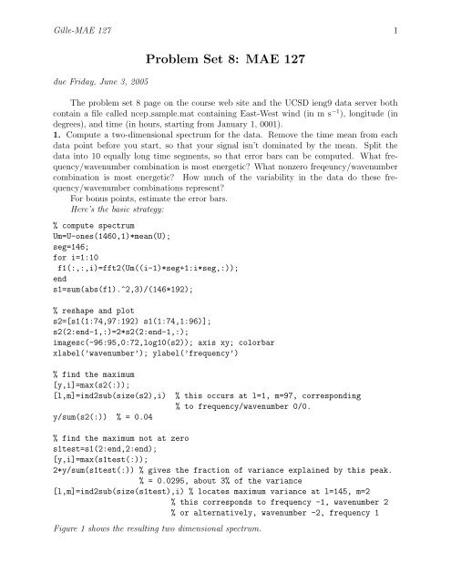
Gille-<strong>MAE</strong> <strong>127</strong> 1<br />
due Friday, June 3, 2005<br />
<strong>Problem</strong> <strong>Set</strong> 8: <strong>MAE</strong> <strong>127</strong><br />
The problem set 8 page on the course web site and the UCSD ieng9 data server both<br />
contain a file called ncep sample.mat containing East-West wind (in m s −1 ), longitude (in<br />
degrees), and time (in hours, starting from January 1, 0001).<br />
1. Compute a two-dimensional spectrum for the data. Remove the time mean from each<br />
data point before you start, so that your signal isn’t dominated by the mean. Split the<br />
data into 10 equally long time segments, so that error bars can be computed. What frequency/wavenumber<br />
combination is most energetic? What nonzero freqeuncy/wavenumber<br />
combination is most energetic? How much of the variability in the data do these frequency/wavenumber<br />
combinations represent?<br />
For bonus points, estimate the error bars.<br />
Here’s the basic strategy:<br />
% compute spectrum<br />
Um=U-ones(1460,1)*mean(U);<br />
seg=146;<br />
for i=1:10<br />
f1(:,:,i)=fft2(Um((i-1)*seg+1:i*seg,:));<br />
end<br />
s1=sum(abs(f1).^2,3)/(146*192);<br />
% reshape and plot<br />
s2=[s1(1:74,97:192) s1(1:74,1:96)];<br />
s2(2:end-1,:)=2*s2(2:end-1,:);<br />
imagesc(-96:95,0:72,log10(s2)); axis xy; colorbar<br />
xlabel(’wavenumber’); ylabel(’frequency’)<br />
% find the maximum<br />
[y,i]=max(s2(:));<br />
[l,m]=ind2sub(size(s2),i)<br />
y/sum(s2(:)) % = 0.04<br />
% this occurs at l=1, m=97, corresponding<br />
% to frequency/wavenumber 0/0.<br />
% find the maximum not at zero<br />
s1test=s1(2:end,2:end);<br />
[y,i]=max(s1test(:));<br />
2*y/sum(s1test(:)) % gives the fraction of variance explained by this peak.<br />
% = 0.0295, about 3% of the variance<br />
[l,m]=ind2sub(size(s1test),i) % locates maximum variance at l=145, m=2<br />
% this corresponds to frequency -1, wavenumber 2<br />
% or alternatively, wavenumber -2, frequency 1<br />
Figure 1 shows the resulting two dimensional spectrum.
Gille-<strong>MAE</strong> <strong>127</strong> 2<br />
70<br />
5<br />
60<br />
4<br />
50<br />
3<br />
frequency<br />
40<br />
30<br />
2<br />
1<br />
20<br />
0<br />
10<br />
−1<br />
0<br />
−80 −60 −40 −20 0 20 40 60 80<br />
wavenumber<br />
−2<br />
Figure 1: Two-dimensional frequency-wavenumber spectrum of zonal wind observations from<br />
the Southern Ocean. Colorscale corresponds to log 10 of spectrum.<br />
To estimate error bars, we use the same method that we used for one-dimensional spectra.<br />
Since the data have been broken into 10 segments, we compute:<br />
nu=2*10;<br />
err_low = nu/chi2inv(1-.05/2,nu); % 0.5853<br />
err_high = nu/chi2inv(.05/2,nu); % 2.0853<br />
This indicates that on a log scale, if the log 10 of the spectrum for a particular frequency–<br />
wavenumber combination is 1, then the uncertainty of this estimate ranges from 0.59 to<br />
2.09. This tells us that peaks that exceed the background spectrum by about 1 unit in log<br />
space are statistically significant.<br />
2. Compute EOFs for the same demeaned data. What fraction of the variance in the data<br />
is explained by the 1st, 2nd, and 3rd mode EOFs?<br />
EOFs are a quick one-line computation.<br />
[u,s,v]=svd(Um);<br />
diag(s(1:3,1:3).^2)/sum(diag(s.^2))<br />
plot(diag(s.^2)/sum(diag(s.^2)))<br />
The fraction of variance is plotted in Figure 2 and the corresponding numerical values indicate<br />
that the first 3 EOFs explain 12.7%, 11.0%, and 9.2% of the variance respectively.<br />
To plot the first mode EOFs in time and space:<br />
subplot(1,2,1);<br />
plot(time-time(1),u(:,1)); xlabel(’time (hours from start of year)’);
Gille-<strong>MAE</strong> <strong>127</strong> 3<br />
0.14<br />
0.12<br />
0.1<br />
fraction of variance explained<br />
0.08<br />
0.06<br />
0.04<br />
0.02<br />
0<br />
0 20 40 60 80 100 120 140 160 180 200<br />
mode number<br />
Figure 2: Fraction of variance explained by EOFs of Southern Ocean wind data.<br />
ylabel(’mode 1 structure’);<br />
subplot(1,2,2);<br />
plot(lon,v(:,1)); xlabel(’longitude’); ylabel(’mode 1 structure’);<br />
The resulting structures in Figure 3 indicate that the leading order response is stronger in<br />
the Pacific Ocean than the Atlantic or Indian Oceans, and that the pattern varies rapidly.
Gille-<strong>MAE</strong> <strong>127</strong> 4<br />
0.06<br />
0.14<br />
0.04<br />
0.12<br />
0.02<br />
0.1<br />
mode 1 structure<br />
0<br />
−0.02<br />
−0.04<br />
mode 1 structure<br />
0.08<br />
0.06<br />
0.04<br />
−0.06<br />
0.02<br />
−0.08<br />
0<br />
−0.1<br />
0 2000 4000 6000 8000 10000<br />
time (hours from start of year)<br />
−0.02<br />
0 100 200 300 400<br />
longitude<br />
Figure 3: Temporal (left) and spatial (right) structure of mode 1 EOF.