SPIE 2010 - SALSA - 3D reconstruction - Bossa Nova Technologies
SPIE 2010 - SALSA - 3D reconstruction - Bossa Nova Technologies
SPIE 2010 - SALSA - 3D reconstruction - Bossa Nova Technologies

Create successful ePaper yourself
Turn your PDF publications into a flip-book with our unique Google optimized e-Paper software.
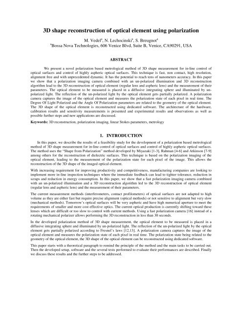
<strong>3D</strong> shape <strong>reconstruction</strong> of optical element using polarization<br />
M. Vedel a , N. Lechocinski a , S. Breugnot a<br />
a <strong>Bossa</strong> <strong>Nova</strong> <strong>Technologies</strong>, 606 Venice Blvd, Suite B, Venice, CA90291, USA<br />
ABSTRACT<br />
We present a novel polarization based metrological method of <strong>3D</strong> shape measurement for in-line control of<br />
optical surfaces and control of highly aspheric optical surfaces. This technique is fast, non contact, high resolution,<br />
alignment free and with unprecedented dynamic. It has the potential to reach tens of nanometers accuracy. In this paper<br />
we show that a polarization imaging camera combined with an un-polarized illumination and <strong>3D</strong> <strong>reconstruction</strong><br />
algorithm lead to the <strong>3D</strong> <strong>reconstruction</strong> of optical element (regular lens and aspheric lens) and the measurement of their<br />
parameters. The optical element to be measured is placed in a diffusive integrating sphere and illuminated by unpolarized<br />
light. The reflection of the un-polarized light by the optical element gets partially polarized. A polarization<br />
camera captures the image of the optical element and measures the polarization state of each pixel in real time. The<br />
Degree Of Light Polarized and the Angle Of Polarization parameters are related to the geometry of the optical element.<br />
The <strong>3D</strong> shape of the optical element is reconstructed using dedicated software. The architecture of the hardware,<br />
calibration results and sensitivity measurements is presented and experimental results and observations as well as<br />
possible further steps and new applications are discussed.<br />
Keywords: <strong>3D</strong> <strong>reconstruction</strong>, polarization imaging, linear Stokes parameters, metrology<br />
1. INTRODUCTION<br />
In this paper, we describe the results of a feasibility study for the development of a polarization based metrological<br />
method of <strong>3D</strong> shape measurement for in-line control of optical surfaces and control of highly aspheric optical surfaces.<br />
The method uses the “Shape from Polarization” method developed by Miyazaki [1-3], Rahman [4-6] and Atkinson [7-9]<br />
among others for the <strong>reconstruction</strong> of dielectric surfaces. This technique is based on the polarization imaging of the<br />
optical element, leading to the measurement of the polarization state for each pixel of the image. This allows the<br />
<strong>reconstruction</strong> of the <strong>3D</strong> shape of the imaged optical element.<br />
With increasing requirement for improving productivity and competitiveness, manufacturing companies are looking to<br />
implement more in-line inspection techniques where the immediate feedback can lead to tighter tolerance, reduction in<br />
scraps and reduction in energy consumption. In this paper, we show that a fast polarization imaging camera combined<br />
with an un-polarized illumination and a <strong>3D</strong> <strong>reconstruction</strong> algorithm led to the <strong>3D</strong> <strong>reconstruction</strong> of optical element<br />
(regular lens and aspheric lens) and the measurement of their parameters.<br />
The current measurement methods (interferometers, contact profilometers) of optical surfaces are not adapted to high<br />
volume as they are either fast but require precise alignment (optical methods) or not sensitive to alignment but very slow<br />
(mechanical methods). Tomorrow’s optical surfaces will be very aspheric and have high numerical aperture to meet the<br />
requirements of smaller and more cost effective optics. The current optical production is currently shifting toward these<br />
lenses which are difficult or too slow to control with current methods. Using a fast polarization camera [16] instead of a<br />
rotating mechanical polarizer allows performing the <strong>3D</strong> <strong>reconstruction</strong> in less than 30 seconds.<br />
In the developed polarization method of <strong>3D</strong> shape measurement, the optical element to be measured is placed in a<br />
diffusive integrating sphere and illuminated by un-polarized light. The reflection of the un-polarized light by the optical<br />
element gets partially polarized according to Fresnel’s laws [12,13]. A polarization camera captures the image of the<br />
optical element and measures the polarization state of each pixel in real time. The polarization state being related to the<br />
geometry of the optical element, the <strong>3D</strong> shape of the optical element can be reconstructed using dedicated software.<br />
This paper starts with a theoretical paragraph to remind the principle of the method and the main tasks to be carried out.<br />
Then the developed setup, software and the several tests performed to evaluate their performances are described. Finally<br />
we discuss these results and the further steps to be addressed.
2. <strong>3D</strong> RECONSTRUCTION BASED ON POLARIZATION IMAGING<br />
2.1 Description of polarization<br />
Light can be totally polarized, unpolarized or partially polarized. A totally polarized light can then be linearly<br />
polarized, circularly polarized, or elliptically polarized. An unpolarized light is a light which has no coherence between<br />
the electric fields along to orthogonal directions. In between light can be partially polarized. The polarization state of<br />
light is usually described using Stokes formalism (Equation 1) [13].<br />
⎡S<br />
S<br />
S r<br />
=<br />
S<br />
⎢⎢⎢⎢<br />
⎣S<br />
0<br />
1<br />
2<br />
3<br />
⎤<br />
⎥⎥⎥⎥<br />
⎦<br />
S<br />
S<br />
S<br />
S<br />
0<br />
1<br />
2<br />
3<br />
=<br />
=<br />
=<br />
=<br />
E E<br />
x<br />
E E<br />
x<br />
E E<br />
x<br />
x<br />
*<br />
x<br />
*<br />
x<br />
*<br />
y<br />
j E E<br />
+ E E<br />
*<br />
y<br />
y<br />
− E E<br />
y<br />
+ E E<br />
y<br />
y<br />
*<br />
y<br />
*<br />
y<br />
*<br />
x<br />
− E E<br />
*<br />
x<br />
= I<br />
= I<br />
= I<br />
o<br />
0<br />
o<br />
0<br />
o<br />
45<br />
= I<br />
+ I<br />
− I<br />
lh<br />
o<br />
90<br />
o<br />
90<br />
− I<br />
− I<br />
o<br />
−45<br />
rh<br />
(1)<br />
It can describe any type of polarization and is linear with the intensity of light which makes it compatible with linear<br />
algebra. The Stokes-Mueller formalism describes mathematically the polarization of light as well as its evolution. This<br />
formalism uses real quadratic values (intensities along horizontal, vertical axes...) directly measured by detectors. A<br />
Stokes vector is a 4 components vector. However, polarization is generally described with more physical parameters.<br />
The parameters relevant for this paper are the Degree Of Linear Polarization (DOLP) and Angle Of linear Polarization<br />
(AOP) (Equation 2). DOLP represents the relative amount of light linearly polarized; AOP represents the orientation of<br />
this linearly polarized part.<br />
DOLP<br />
=<br />
S<br />
1<br />
+ iS<br />
S<br />
0<br />
2<br />
2.2 Fresnel equations<br />
1<br />
AOP = Arg( S1<br />
+ iS<br />
2<br />
)<br />
(2)<br />
2<br />
Generally speaking, polarization of light will be modified after interacting with an object [12,13]. The possible<br />
modifications include, but are not limited to, depolarization of a polarized light and polarization of an unpolarized light.<br />
Polarization of an unpolarized light is a very general phenomenon. It comes from a difference in the reflection<br />
coefficient for the electric field in the plane of incidence and perpendicular to the plane of incidence. This difference in<br />
the reflection coefficient is perfectly determined by the angle of incidence on the surface and the physical properties of<br />
the material. The reflection coefficient for the electric field in the plane of incidence (p-polarization) and perpendicular<br />
to the plane of incidence (s-polarization) are calculated using the Fresnel equations [12]. The fact that the reflection<br />
coefficients are not the same makes that an unpolarized light will become partially s-polarized after a reflection by a<br />
dielectric surface (figure 1). Using the Fresnel equations, the DOLP can be calculated for any angle of incidence θ<br />
(Equation 3). The calculation of the DOLP after a specular reflection of light by a dielectric surface shows that a<br />
measurement of DOLP can be inverted to two possible angles of incidence with the hypothesis of a known material<br />
refractive index and unpolarized incident light [1-11]. The same calculation can be conducted for other surfaces<br />
materials. Morel described an extension of the “Shape from Polarization” method to metallic surfaces using a complex<br />
refractive index [10,11].
2 2 2 2 2 4<br />
2sin θ n −sin<br />
θ −n<br />
sin θ −sin<br />
θ<br />
DOLP reflection<br />
=<br />
(3)<br />
2 2 2 2<br />
4<br />
n −sin<br />
θ − n sin θ − 2sin θ<br />
Figure 1. Fresnel laws: light reflected by a dielectric surface becomes partially polarized depending on the incidence angle<br />
2.3 Shape from polarization<br />
Gradient field estimation<br />
Given a conventional Cartesian coordinate system (X,Y,Z) one can express the <strong>3D</strong> shape by the height Z in<br />
function of (X,Y) parameters. The method presented in this paper is based on the surface gradient field <strong>reconstruction</strong><br />
and its numerical integration. Figure 2 shows the geometrical parameters. Each normal vector (Equation 3) is expressed<br />
knowing the local slope, related to the zenith angle θ i (incidence angle of the light), and the azimuth angle φ [1-11].<br />
Partially<br />
polarized light<br />
DOLP(θ i )<br />
AOP(φ)<br />
X<br />
N r Unpolarized<br />
θ r illumination<br />
θ i<br />
φ<br />
Y<br />
⎛ ∂Z(<br />
X , Y ) ⎞<br />
−<br />
⎛ p = tan( θ )cos( ϕ)<br />
⎞ ∂<br />
r ∂Z(<br />
X , Y )<br />
= = tan( )sin( ) = −<br />
⎜⎜⎜<br />
⎟⎟⎟<br />
∂Y<br />
⎝ 1 ⎠ 1<br />
⎜⎜⎜⎜⎜⎜<br />
X (3)<br />
N q θ ϕ<br />
⎟⎟⎟⎟⎟⎟<br />
⎝<br />
⎠<br />
Figure 2. Geometrical parameters
Considering a specular reflection on the surface element the incidence angle θ i and the reflected angle θ r are the same.<br />
We will denote it the zenith angle θ. The Fresnel equations link the surface’s local slope (zenith angle), the refractive<br />
index n of the material and the Degree Of Linear Polarization (Equation 3). This equation can be inverted to express the<br />
two zenith angles θ possible: one below and one above the Brewster incidence angle (figure 1). In most of the cases, the<br />
first root will be the right one. For a usual glass with refractive index around 1.5, Brewster’s angle is 56°. Most of the<br />
optics do not have such high slope. Even high numerical apertures aspherics or condensers have slopes below 45° at their<br />
edge. The results presented in this paper are limited to these cases.<br />
The second parameter φ is related to the Angle Of Polarization. As the polarization vector is defined within [0°; 180°]<br />
cycle there are two possible azimuth angles for the normal vector (Equation 4).<br />
ϕ = AOP or ϕ = AOP + π<br />
(4)<br />
Several methods to resolve that ambiguity have been described in previous papers [1-11]. A simple algorithm has been<br />
used to disambiguate the normal to the surface. As shown in figure 3, for simple lenses shape, the normal to the surface<br />
appear to radiate for the point of the lens oriented toward the lens. The angle θ also increases with the radius. These are<br />
the properties used to disambiguate the normal to the surface for simple shape lenses: convex or concave surfaces with<br />
no inflexion point.<br />
Gradient field integration<br />
Once the zenith and the azimuth angles are known for each pixel of the imaged sample we need to operate a<br />
numerical integration in order to obtain the <strong>3D</strong> height map Z(X,Y). Many off the shelf algorithms to project a gradient<br />
field onto the closest integrable gradient field and to recover the <strong>3D</strong> surface associated with this gradient field exist. The<br />
most used is the Frankot-Chellapa algorithm [14]. The non integrable gradient field measured is projected onto a base of<br />
integrable functions which are the Fourier functions. Let us denote Z ~ , p ~ and q ~ the Fourier transform of respectively<br />
the height map and the X, Y components of the gradient field; µ and ν the reciprocal coordinates in the Fourier space.<br />
Then the Fourier transform of the height map can be expressed as Equation (4) for each pixel.<br />
* ~ *<br />
~ − i.<br />
µ .<br />
~<br />
p − i . ν . q<br />
Z ( µ , ν ) =<br />
(4)<br />
2 2<br />
µ + ν<br />
Finally an inverse Fourier transform operation is computed in order to obtain the height map of the sample’s surface.<br />
This algorithm is very efficient in term of both precision of the results and speed.<br />
3.1 Illumination design<br />
3. EXPERIMENTAL SETUP<br />
As we measure the amount of polarized light reflected by the sample to be characterized, an unpolarized<br />
illumination had to be designed. It is based on an integrating sphere which uses a white Lambertian coating. The light<br />
source used is made of 2 green LEDs. These LEDs were chosen for several reasons: first of all, they provide high<br />
luminous flux, typically 160 lm per LED. They have a narrow spectrum, which is an advantage as the polarization<br />
elements used in the polarization camera presents some chromatic dependency of its polarization properties. Figure 3<br />
shows pictures of the sphere.
Figure 3. Picture of the integrating sphere (a) Closed (b) Open with illumination<br />
3.2 Polarization camera<br />
The polarization camera used is composed of a fast polarization modulator developed by <strong>Bossa</strong> <strong>Nova</strong> <strong>Technologies</strong><br />
[16]. It allows switching polarization state between 4 linear polarization states (0°, 45°, 90° and 135°). The camera is<br />
able to perform polarization imaging of a scene. With the 4 polarization images acquired in real time, it is easy to<br />
calculate the linear Stokes parameters and the following polarization parameters - Degree of Linear Polarization (DOLP)<br />
and the Angle of Polarization (AOP) – for each pixel of the image. The polarization camera is based on a standard CCD<br />
camera. This CCD camera has good capacity, resolution, noise and linearity. Figure 4 shows the polarization camera<br />
mounted vertically to image the sample that is mounted inside the integrating sphere.<br />
Figure 4. (a) <strong>Bossa</strong> <strong>Nova</strong> <strong>Technologies</strong> linear Stokes camera <strong>SALSA</strong> TM (b) DOLP grayscale image of a 1’’ aspheric lens (c) AOP as a<br />
color HUE<br />
The DOLP is increasing with the radius, as the slope of the optic is; the AOP is varying according to the azimuth angle.<br />
3.3 Sample mount<br />
The measurement is based on the analysis of the light reflected by the first surface of the sample. To be able to<br />
measure only the light reflected by the first surface, it is necessary to remove any other reflected and scattered light<br />
coming from the back surface of the sample or from the holder. The sample needs to be both opaque and non scattering.<br />
This can be achieved by index matching the back surface of lens to the support. In this case, the support must have the<br />
same refractive index as the lens. The best to this end is to use an absorptive glass optical density and index matching<br />
liquid (figure 5).
Figure 5: (a) the specular reflection at an air-glass interface is characterized by a 4% reflection coefficient. (b) Using an optical density<br />
as a support avoids both transmitted and scattered light. (c) Index matching the optical density and the lens eliminates the surface<br />
reflections<br />
We used an index matching liquid of refractive index n=1.52. The refractive index of BK7 (most commonly used glass)<br />
is exactly this value around 520nm (green). To test the efficiency of the set up, we imaged the lens on the absorptive<br />
neutral density without index matching liquid, with water (refractive index 1.33) as index matching material and finally<br />
with the index matching material (figure 6). Without index matching material, a strong back reflection is visible. It is<br />
even brighter than the front reflection because it comes from the interface between the lens and air and from the interface<br />
between the absorptive neutral density and air. Interferences fringes are visible on the back surface reflection (equal<br />
thickness interference fringes). The reflections at the back surface are about to 8% of the total light which is twice as<br />
much as the front surface reflection. With water as index matching material, the back surface reflections are highly<br />
attenuated but are still not negligible in front on the front surface reflection. The total reflection coefficient is about<br />
0.9%. With the index matching liquid, the back reflection totally disappears; only the front surface reflection is visible.<br />
Figure 6: (a) lens on an absorptive optical density. The back surface reflection is stronger than front surface reflection. (b) Using water<br />
as index matching material dramatically reduces back surface reflection. (c) Using a specific index matching liquid totally eliminates<br />
the back surface reflection<br />
3.4 Full Setup<br />
Figure 7 shows a picture of the complete system, showing the polarization camera, the integrating sphere and the<br />
sample.
Polarization camera<br />
Integrating sphere<br />
Sample<br />
Illumination LEDs<br />
Figure 7. Full Setup<br />
4. TESTS ON COMMERCIAL SAMPLES - ANALYSIS<br />
In order to evaluate the performances and the limitations of the developed system we realized many tests on several<br />
spherical and aspheric commercial samples. Measurements were performed on spherical lenses with Radius of Curvature<br />
ranging from 15mm to 110mm. Profiles can be deduced from the <strong>3D</strong> shape and compared to theoretical values. The<br />
repeatability of the measurement can be evaluated by subtracting two measurements. Figure 8 shows a screenshot of a<br />
sample’s surface <strong>3D</strong> <strong>reconstruction</strong> (a), the selection of a section profile to be plotted (b) and an extracted profile (c).<br />
Figure 8. (a)Reconstructed surface, (b) section (c) extracted profile<br />
4.1 Tests on commercial samples<br />
Profile measurements<br />
Profile measurements were performed on commercial highly aspheric lenses. These profiles were compared to<br />
very accurate measured profiles (performed with 250nm resolution mechanical profilometer) given by the constructor in<br />
order to evaluate the performances of the system. Figure 9 shows a profile measured on a commercial aspheric lens<br />
sample with a high departure from sphere parameter (conic constant: k = -2.27, Departure From Sphere=180µm). The<br />
red curve shows the profile acquired by the constructor’s contact profilometer (1nm resolution) and the black curve<br />
shows the one acquired by our system.
Theoretical and BNT Profiles<br />
0.5<br />
0<br />
-15 -10 -5 0 5 10 15<br />
-0.5<br />
-1<br />
Height (mm)<br />
-1.5<br />
-2<br />
-2.5<br />
-3<br />
Theoretical Profile<br />
-3.5<br />
BNT profile<br />
-4<br />
X section (mm)<br />
Figure 9: Measured and theoretical profiles – aspheric sample<br />
One can notice the strong artifact at the top of the surface. It is due to the reflection of the diaphragm on the sample<br />
surface which modifies the DOLP value. The DOLP is already very low on the central area of the sample because the<br />
incident angle of the light beam is very close to the normal direction. So the combination of those two parameters leads<br />
to that strong artifact. Figure 10 shows the plot of the difference between the reconstructed and the theoretical profile. If<br />
we forget the strong artifact at the center due to the reflection of the pupil lens on the sample we can notice that the error<br />
is a slowly increasing in the field and has a rotational symmetry component. The maximum amplitude is around 25µm at<br />
the edge of the sample. There is a strong field dependency. However, we think that dependency is an artifact and does<br />
not show the real limitation of the <strong>reconstruction</strong> method. The real limitation is more likely to be the high frequency<br />
noise around the slow variation. The amplitude of that noise is about 100nm which correspond to the order of magnitude<br />
given by our previous simulations. In the following section we will analyze the possible sources of these artifacts.<br />
Figure 10. Difference between the theoretical and the reconstructed profile
Repeatability<br />
Several measurements in a row were performed on the same sample (removing the sample from the holder) in<br />
order to evaluate the repeatability of the results. Reconstructed surfaces of two successive acquisitions are subtracted.<br />
Residual noise and artifacts can be estimated. Figure 11 shows the <strong>3D</strong> residual noise of two measurements on a 20.6mm<br />
ROC sample (sample removed between the 2 measurements). The PV value of the residual surface is 1.9µm. This is<br />
extremely encouraging as the measurements are done without any specific optical alignment like the ones required for<br />
interferometric methods.<br />
Figure 11. Measurement repeatability<br />
5. CURRENT LIMITATIONS – FURTHER STEPS<br />
These preliminary tests were very useful to estimate the limitations of the system. The main limitations are the<br />
artifact due to the central reflection and the slow deviation observed which is increasing with the field of view. The<br />
potential sources of errors investigated are listed below:<br />
Artifacts in the <strong>3D</strong> <strong>reconstruction</strong> algorithm itself<br />
The measurement of DOLP and AOP parameters<br />
5.1 Artifacts introduced by the algorithm<br />
The point is to evaluate the error introduced by the <strong>reconstruction</strong> algorithm itself. We generated perfect DOLP and<br />
AOP map and used the <strong>reconstruction</strong> algorithm. Then we can compare the reconstructed spheres with a theoretical<br />
sphere and see the defects introduced by the algorithm. Then we have computed the difference between the reconstructed<br />
shape and the theoretical one. Figure 12 shows the <strong>3D</strong> plot and an extracted profile of that difference
Difference and fitting<br />
0.00E+00<br />
-1.50E+01 -1.00E+01 -5.00E+00 0.00E+00 5.00E+00 1.00E+01 1.50E+01<br />
Amplitude of the difference (mm)<br />
-5.00E-04<br />
-1.00E-03<br />
-1.50E-03<br />
-2.00E-03<br />
-2.50E-03<br />
-3.00E-03<br />
X section (mm)<br />
Difference Perfect sphere -<br />
Reconstructed shere<br />
Fitting with a spherical profile<br />
Figure 12: <strong>3D</strong> plot (a) and profile (b) of the deviation between perfect sphere and reconstructed sphere<br />
The PV amplitude of the deviation is around 2.7µm for a simulated 40 mm Radius Of Curvature. Moreover the profile<br />
shape of the deviation appears to be spherical and using a numerical solver we can estimate the best sphere parameters<br />
which fit the deviation profile (especially the Radius Of Curvature of the deviation profile). Figure 13 shows that the<br />
ROC of the deviation profile is proportional to the ROC of the sphere to be reconstructed.<br />
ROC of the deviation profile vs. ROC of<br />
theoretical sphere<br />
35000<br />
30000<br />
ROC defect (mm)<br />
25000<br />
20000<br />
15000<br />
10000<br />
5000<br />
0<br />
0 10 20 30 40 50 60<br />
ROC perfect sphere (mm)<br />
Figure 13: ROC of the profile deviation vs. ROC of the sphere<br />
These tests have shown that the algorithm itself introduces artifact in the <strong>3D</strong> reconstructed shape. Those artifacts strongly<br />
depend on the geometric parameters of the system. The PV amplitude of the defect ranges from 2 to 4µm depending on<br />
the Radius Of Curvature of the sphere and on geometrical parameters. The <strong>reconstruction</strong> process assumes that the<br />
distance between the entrance pupil and the sample as well as the magnification of the optical conjugation is uniform. In<br />
reality, as shown in figure 14, these parameters vary in the field. This is particularly true with high sag optics such as the<br />
tested aspherics. That explains why the ROC of the deviation profile is increasing with the ROC of the sphere to be<br />
reconstructed. The more the ROC of the sphere is, the less the sag is, and the less the amplitude of the deviation is. The<br />
consequences are a non uniform integration of the gradient field and could lead to such an artifact. The same kind of<br />
error has been observed in the measurement of the DOLP parameter; it will be detailed in the following section.
∆d<br />
Sample<br />
Lens<br />
Detector<br />
Distance<br />
Distance + ∆d<br />
Figure 14 Non uniformity of the distance Sample – Entrance pupil<br />
5.2 Measurement of DOLP and AOP parameters<br />
Measured DOLP profiles were compared to theoretical DOLP. As shown on Figure 15 the measured DOLP are<br />
always smaller than expected values while the field is increasing. The DOLP error is up to 0.11 at the edge (11% DOLP).<br />
It has a strong impact on the final result as it is related to the local slope of the surface. That error is due to an important<br />
amount of flare light in the setup.<br />
Figure 15: (a) Measured and Theoretical DOLP profiles, 1’’ spherical commercial sample, ROC=20.6mm; (b) Deviation<br />
If we call I 0 the intensity of the flare light, I S and I P respectively the intensity of s-polarized and p-polarized light,<br />
DOLP mes and DOLP th respectively the measured and the theoretical DOLP, we can see the effect on the DOLP<br />
deviation:<br />
∆<br />
∆<br />
DOLP<br />
DOLP<br />
=<br />
=<br />
DOLP<br />
I<br />
S<br />
measured<br />
I<br />
0<br />
+ I + 2 I<br />
P<br />
− DOLP<br />
0<br />
× DOLP<br />
theoretica l<br />
2 (4)<br />
th<br />
= K × DOLP<br />
theoretica l
That leads to a DOLP error proportional to the DOLP expected value. That assumption was verified experimentally. The<br />
K constant depends only on the amount of flare light which is related to the experimental setup. Therefore it is possible<br />
to measure it and then to correct systematically the DOLP error. That compensation was implemented and gave excellent<br />
results. Figure 16 shows corrected DOLP and the new deviation. The error was put down 0.4% pic-to-valley.<br />
Figure 16 : Calibrated an theoretical DOLP, 1’’ spherical commercial sample, ROC=20.6mm; (b) Deviation<br />
Similar results have been observed on commercial spherical and aspheric optics with Radius Of Curvature ranging<br />
between 15mm to 105mm. The DOLP correction performed here does not take into account any field dependency. The<br />
next step should be to perform a complete calibration of DOLP and AOP values using an angle controlled reflecting<br />
plane. Then we could build a calibration matrix for each angle. The real noise appears as a high frequency modulation of<br />
the symmetric remaining artifact. Its amplitude is around 100nm.<br />
6. CONCLUSION<br />
The principle of a polarization imaging system for <strong>3D</strong> <strong>reconstruction</strong> of optical elements was successfully<br />
demonstrated. A complete setup based on an unpolarized illumination and <strong>Bossa</strong> <strong>Nova</strong> <strong>Technologies</strong>’ linear Stokes<br />
polarization camera was designed. A dedicated <strong>reconstruction</strong> algorithm based on the off-the-shelf Frankot-Chellapa<br />
algorithm was developed and tested on several commercial samples. The described setup performances were evaluated<br />
by comparing measured section profiles and theoretical profiles given by constructors. The samples tested with the<br />
method were one and two inches diameters, spherical and aspheric, with Radius of Curvature ranging from 15mm to<br />
110mm and Departure From Sphere ranging from 0 to 800µm. The best accuracy obtained was 25µm with this setup.<br />
This is very encouraging as the current setup was based on relatively cheap components and no specific calibrations or<br />
signal/image processing was performed.<br />
This work has been sponsored by a SBIR phase I grant from the National Science Foundation.<br />
REFERENCE<br />
[1] Miyazaki, D., Tan, R. T., Hara, K., Ikeuchi, K., 2003. “Polarization-based Inverse Rendering from a Single View”.<br />
IEEE Int. Conf. on Computer Vision, Nice, France, vol. II, pp. 982-987, (2003).<br />
[2] Miyazaki D., Takashima N., Yoshida A. Hara E. Ikeuchi K. "Polarization-based Shape Estimation of Transparent<br />
Objects by Using Raytracing and PLZT Camera", Proceedings of <strong>SPIE</strong> (Polarization Science and Remote Sensing<br />
II, Part of <strong>SPIE</strong>'s International Symposium on Optics and Photonics 2005), Vol. 5888, pp. 1-14, San Diego, CA<br />
USA, Aug. 2005, (2005)<br />
[3] Miyazaki, D., “Calculation of surface orientations of transparent objects by little rotation using polarization”, Senior<br />
Thesis submitted to the Department of Information Science on February 15, 2000
[4] S. Rahmann, “Inferring 3d scene structure from a single polarization image,” in Conference on Polarization and<br />
Color Techniques in Industrial Inspection, volume 3826 of <strong>SPIE</strong> Proceedings, pp. 22–33, June 99.<br />
[5] Rahmann, S., Canterakis, N., 2001. “Reconstruction of Specular Surfaces using Polarization Imaging”. Int. Conf. on<br />
Computer Vision and Pattern Recognition, Kauai, USA, vol. I, pp. 149-155, (2001).<br />
[6] S. Rahmann and N. Canterakis, “Reconstruction of specular surfaces using polarization imaging,” in IEEE<br />
Computer Vision and Pattern Recognition (CVPR01), volume I, Kauai, USA, pp. 149–155, December 2001.<br />
[7] Atkinson Gary A., Edwin R. Hancock, “Multi-view Surface Reconstruction using Polarization”, Department of<br />
Computer Science, University of York, IEEE International Conf. on Computer Vision, (2005)<br />
[8] Atkinson Gary A., Edwin R. Hancock, “Recovery of Surface Orientation From Diffuse Polarization”, Department of<br />
Computer Science, University of York, IEEE Transaction on image processing, Vol. 15, n°6, (June 2006)<br />
[9] Atkinson Gary A., “Surface Shape and Reflectance Analysis Using Polarization”, submitted for the degree of Doctor<br />
of Philosophy, Department of Computer Science, University of York, May 2007, (2007).<br />
[10] Morel Olivier, Meriaudeau Fabrice, Stolz Christophe, Gorria Patrick, “Polarization Imaging Applied to <strong>3D</strong><br />
Reconstruction of Specular Metallic Surfaces”, in Machine Vision Applications in Industrial Inspection XIII; Jeffery<br />
R. Price, Fabrice Meriaudeau; eds., Proc. <strong>SPIE</strong> 5679, 178–186 (San Jose, California, USA, 2005).<br />
[11] Morel Olivier, Meriaudeau Fabrice, Stolz Christophe, Gorria Patrick, “Active Lighting Applied to <strong>3D</strong><br />
Reconstruction of Specular Metallic Surfaces by Polarization Imaging”, Thesis Olivier Morel, Le2i UMR CNRS<br />
5158, 12 rue de la Fonderie, 71200 Le Creusot, France, Optical Society of America (2005).<br />
[12] L. B.Wolff and T. E. Boult, “Constraining object features using a polarization reflectance model,” IEEE Trans.<br />
Pattern Anal. Machine Intell. 13, 635–657 (1991).<br />
[13] S. Huard, “Polarized optical wave,” in Polarization of Light (Wiley, 1997).<br />
[14] Frankot Robert T., Chellappa Rama, “A Method for Enforcing Integrability in Shape from Shading Algorithms”<br />
IEEE Transactions on pattern analysis and machine intelligence, Vol. 10, n°4, July 1988<br />
[15] J.Scott Tyo, Dennis L. Goldstein, David B. Chenault, Joseph A. Shaw, ”Review of passive imaging polarimetry for<br />
remote sensing applications”, Applied Optics 5453, Vol. 45, No. 22, (2006)<br />
[16] Lefaudeux N., Lechocinski N., Breugnot S., Clemenceau, P, <strong>Bossa</strong> <strong>Nova</strong> <strong>Technologies</strong>, “Compact and robust linear<br />
Stokes polarization camera”, <strong>SPIE</strong> conference, Polarization: Measurement, Analysis, and Remote Sensing VIII,<br />
Volume 6972, 2008