EMPIRE Manual

EMPIRE Manual
(c) IMST GmbH 1998-2006
October 19, 2006

User and Reference Manual
for the
3D-EM Time Domain Simulator
EMPIRE XCcel TM
c○IMST GmbH
Carl-Friedrich-Gauß-Str. 2 • D-47475 Kamp-Lintfort, Germany
Phone +49 (0) 2842 / 981 100 • Fax +49 (0) 2842 / 981 199
E-Mail: empire.support@imst.de. Internet: www.empire.de
i (C) 2006

Copyright notice
Copyright c○1998-2006 IMST GmbH. All rights reserved. No part of the EMPIRE XCcel TM software, that needs a
license, may be used without a valid license from the IMST.
THERE IS NO WARRANTY, TO THE EXTENT PERMITTED BY APPLICABLE LAW. EXCEPT WHEN OTH-
ERWISE STATED IN WRITING THE COPYRIGHT HOLDERS AND/OR OTHER PARTIES PROVIDE THE
PROGRAM ”AS-IS” WITHOUT WARRANTY OF ANY KIND, EITHER EXPRESSED OR IMPLIED, INCLUDING,
BUT NOT LIMITED TO, THE IMPLIED WARRANTIES OF MERCHANTABILITY AND FITNESS FOR A
PARTICULAR PURPOSE.
THE ENTIRE RISK AS TO THE QUALITY AND PERFORMANCE OF THE PROGRAM IS WITH YOU. SHOULD
THE PROGRAM PROVE DEFECTIVE, YOU ASSUME THE COST OF ALL NECESSARY SERVICING, REPAIR
OR CORRECTION.
Please pay attention to the following facts
• EMPIRE XCcel TM is a trademark of IMST GmbH.
• EMPIRE XCcel TM makes use of public software which has to be distributed with the EMPIRE XCcel TM software.
This includes among others
1. The tcl/tk GUI system
2. Gnuplot, Emacs and other GNU–Software
The sources of the public programs including the appropriate license files can be found on the EMPIRE XCcel TM
CD-ROM /pd_sources.
ii (C) 2006

Preface
EMPIRE XCcel TM is an established and versatile electromagnetic field simulator based upon the Finite-Difference Time-
Domain Method (FDTD). At the IMST GmbH, this powerful method has been applied to build an Electro Magnetic field
simulator for the analysis of Packages, Interconnects, Radiators, waveguide Elements (EMPIRE XCcel TM ) and EMC
problems.
The exact knowledge of electromagnetic fields and the propagation of waves is a prerequisite for the design of radio
frequency (RF) elements. In former times, RF design tasks were based on measurement and simple models, leading
to time and costs consuming design procedures. Today, affordable computer hard- and software have established and
simulation programs can accurately predict the electromagnetic behavior of new products. So, field simulators have
become a new standard for RF calculations.
Unlike the Finite Element Method, which has long been established in computing electromagnetic fields, the FDTD
method had its breakthrough in the late 80’s when extensive research and development lead to a number of improvements
in applying advanced boundary conditions, e.g. free space or waveguides, and, therefore, reducing significantly the area
of simulation. Today, its applicability covers the whole area of three-dimensional (3D) field simulations for RF designer.
Originally intended to analyze planar passive structures, the EMPIRE XCcel TM simulator was continuously extended
to capture more and more high frequency applications. It has proven its functionality in numerous comparisons with
measurements and was successfully applied in many different microwave component designs. The method is based
on the most efficient algorithm known which is very accurate and simplification is hardly necessary since it solves the
discretized Maxwell’s equations directly.
The EMPIRE XCcel TM Graphical User Interface works on all supported Platforms, like Windows NT/2000/XP, Suse and
Red Hat Linux. Graphics data can be easily exchanged with other CAD programs for both 2D layout data (DXF 12,
Gerber, GDSII, ...) as well as 3D structures in STL standard which is supported by nearly all CAD tools. Multiple port
scattering parameters, radiation patterns, field plots etc. are generated for a user defined frequency range within only one
simulation process. Monitoring and animation can give physical insight into the electromagnetic wave phenomena while
accurate results are obtained with little effort.
iii (C) 2006

About this manual
This manual is divided into several parts, intended to guide both very beginners and skilled experts from installation and
simulation setup to understanding and exploiting the results.
• Part I describes the installation and licensing process.
• Part II describes the EMPIRE XCcel TM Graphical User Interface, the simulation control as well as pre- and postprocessing
features.
• Part III is the User interface reference, a complete description of all actions, operations, options and simulation
parameters of EMPIRE XCcel TM .
• Part IV describes the theoretical background of the applied method. A skilled user can skip this part, if he is
already familiar with FDTD.
Any comments and suggestions related to this manual are highly appreciated and should be mailed to
empire.support@imst.de. Manual updates can be down-loaded as pdf-files from the web at www.empire.de.
iv (C) 2006

Contents
I Software Administration 6
1 Installation on Windows PC 7
1.1 Requirements for PC Installation . . . . . . . . . . . . . . . . . . . . . . . . . . . . . . . . . . . . . 7
1.2 Installation Procedure . . . . . . . . . . . . . . . . . . . . . . . . . . . . . . . . . . . . . . . . . . . 7
2 License Setup 14
2.1 Request a License . . . . . . . . . . . . . . . . . . . . . . . . . . . . . . . . . . . . . . . . . . . . . 14
2.2 Install the License . . . . . . . . . . . . . . . . . . . . . . . . . . . . . . . . . . . . . . . . . . . . . 15
3 Floating License on Windows 18
3.1 Installation on the Server . . . . . . . . . . . . . . . . . . . . . . . . . . . . . . . . . . . . . . . . . 18
3.2 Installation on each Client . . . . . . . . . . . . . . . . . . . . . . . . . . . . . . . . . . . . . . . . . 18
4 Support 20
4.1 Web Sites . . . . . . . . . . . . . . . . . . . . . . . . . . . . . . . . . . . . . . . . . . . . . . . . . 20
4.2 Contact Us . . . . . . . . . . . . . . . . . . . . . . . . . . . . . . . . . . . . . . . . . . . . . . . . . 20
4.3 License Diagnostic . . . . . . . . . . . . . . . . . . . . . . . . . . . . . . . . . . . . . . . . . . . . 20
5 Linux systems 22
5.1 Requirements . . . . . . . . . . . . . . . . . . . . . . . . . . . . . . . . . . . . . . . . . . . . . . . 22
5.2 Installation . . . . . . . . . . . . . . . . . . . . . . . . . . . . . . . . . . . . . . . . . . . . . . . . . 22
5.3 Start Commands . . . . . . . . . . . . . . . . . . . . . . . . . . . . . . . . . . . . . . . . . . . . . . 23
5.4 License Request . . . . . . . . . . . . . . . . . . . . . . . . . . . . . . . . . . . . . . . . . . . . . . 23
5.5 Install the License . . . . . . . . . . . . . . . . . . . . . . . . . . . . . . . . . . . . . . . . . . . . . 23
II Empire User Interface 24
6 Introduction 25
6.1 Top tool bars . . . . . . . . . . . . . . . . . . . . . . . . . . . . . . . . . . . . . . . . . . . . . . . . 26
6.2 Control Lists . . . . . . . . . . . . . . . . . . . . . . . . . . . . . . . . . . . . . . . . . . . . . . . . 28
6.3 Bottom line . . . . . . . . . . . . . . . . . . . . . . . . . . . . . . . . . . . . . . . . . . . . . . . . 28
1 (C) 2006

CONTENTS 2
7 Templates 30
7.1 Transmission Lines & Waveguides . . . . . . . . . . . . . . . . . . . . . . . . . . . . . . . . . . . . 30
7.2 SMD chip components . . . . . . . . . . . . . . . . . . . . . . . . . . . . . . . . . . . . . . . . . . 31
7.3 RLC . . . . . . . . . . . . . . . . . . . . . . . . . . . . . . . . . . . . . . . . . . . . . . . . . . . . 31
7.4 Antennas . . . . . . . . . . . . . . . . . . . . . . . . . . . . . . . . . . . . . . . . . . . . . . . . . . 31
7.5 Examples . . . . . . . . . . . . . . . . . . . . . . . . . . . . . . . . . . . . . . . . . . . . . . . . . 33
8 Parameter Set-up 34
8.1 Geometry . . . . . . . . . . . . . . . . . . . . . . . . . . . . . . . . . . . . . . . . . . . . . . . . . 34
8.2 Frequency . . . . . . . . . . . . . . . . . . . . . . . . . . . . . . . . . . . . . . . . . . . . . . . . . 35
8.3 Prototype . . . . . . . . . . . . . . . . . . . . . . . . . . . . . . . . . . . . . . . . . . . . . . . . . . 35
8.4 Simulation . . . . . . . . . . . . . . . . . . . . . . . . . . . . . . . . . . . . . . . . . . . . . . . . . 36
8.5 Boundary conditions . . . . . . . . . . . . . . . . . . . . . . . . . . . . . . . . . . . . . . . . . . . . 36
8.6 Autodisc . . . . . . . . . . . . . . . . . . . . . . . . . . . . . . . . . . . . . . . . . . . . . . . . . . 37
8.7 Advanced Simulation Parameters . . . . . . . . . . . . . . . . . . . . . . . . . . . . . . . . . . . . . 37
9 Object creation 42
9.1 Box . . . . . . . . . . . . . . . . . . . . . . . . . . . . . . . . . . . . . . . . . . . . . . . . . . . . 42
9.2 Polygon . . . . . . . . . . . . . . . . . . . . . . . . . . . . . . . . . . . . . . . . . . . . . . . . . . 43
9.3 Line Polygon . . . . . . . . . . . . . . . . . . . . . . . . . . . . . . . . . . . . . . . . . . . . . . . 44
9.4 Bond Wire . . . . . . . . . . . . . . . . . . . . . . . . . . . . . . . . . . . . . . . . . . . . . . . . . 44
9.5 Circle . . . . . . . . . . . . . . . . . . . . . . . . . . . . . . . . . . . . . . . . . . . . . . . . . . . 45
9.6 Segment of a circle . . . . . . . . . . . . . . . . . . . . . . . . . . . . . . . . . . . . . . . . . . . . 45
9.7 Sphere . . . . . . . . . . . . . . . . . . . . . . . . . . . . . . . . . . . . . . . . . . . . . . . . . . . 46
9.8 Rotational Polygon . . . . . . . . . . . . . . . . . . . . . . . . . . . . . . . . . . . . . . . . . . . . 46
9.9 2D Layout Import . . . . . . . . . . . . . . . . . . . . . . . . . . . . . . . . . . . . . . . . . . . . . 46
9.10 3D Solid Import . . . . . . . . . . . . . . . . . . . . . . . . . . . . . . . . . . . . . . . . . . . . . . 47
9.11 2D Point List Import . . . . . . . . . . . . . . . . . . . . . . . . . . . . . . . . . . . . . . . . . . . . 48
9.12 Python Scripts . . . . . . . . . . . . . . . . . . . . . . . . . . . . . . . . . . . . . . . . . . . . . . . 48
10 Object modification 50
11 Operations 51
11.1 Operators . . . . . . . . . . . . . . . . . . . . . . . . . . . . . . . . . . . . . . . . . . . . . . . . . 51
11.2 Select objects . . . . . . . . . . . . . . . . . . . . . . . . . . . . . . . . . . . . . . . . . . . . . . . 52
11.3 Move Objects . . . . . . . . . . . . . . . . . . . . . . . . . . . . . . . . . . . . . . . . . . . . . . . 52
11.4 Copy Objects . . . . . . . . . . . . . . . . . . . . . . . . . . . . . . . . . . . . . . . . . . . . . . . 54
11.5 Stretch Objects . . . . . . . . . . . . . . . . . . . . . . . . . . . . . . . . . . . . . . . . . . . . . . . 56
11.6 Boolean operations . . . . . . . . . . . . . . . . . . . . . . . . . . . . . . . . . . . . . . . . . . . . 58
12 Object properties 59
12.1 Basic Object Properties . . . . . . . . . . . . . . . . . . . . . . . . . . . . . . . . . . . . . . . . . . 60
12.2 Circuit Elements . . . . . . . . . . . . . . . . . . . . . . . . . . . . . . . . . . . . . . . . . . . . . . 62
12.3 Field . . . . . . . . . . . . . . . . . . . . . . . . . . . . . . . . . . . . . . . . . . . . . . . . . . . . 62
12.4 Advanced Properties . . . . . . . . . . . . . . . . . . . . . . . . . . . . . . . . . . . . . . . . . . . . 66
(C) 2006

CONTENTS 3
13 Port types 72
13.1 Coaxial Port . . . . . . . . . . . . . . . . . . . . . . . . . . . . . . . . . . . . . . . . . . . . . . . . 72
13.2 Square coaxial Port . . . . . . . . . . . . . . . . . . . . . . . . . . . . . . . . . . . . . . . . . . . . 74
13.3 Coplanar Port . . . . . . . . . . . . . . . . . . . . . . . . . . . . . . . . . . . . . . . . . . . . . . . 75
13.4 Lumped Port . . . . . . . . . . . . . . . . . . . . . . . . . . . . . . . . . . . . . . . . . . . . . . . . 76
13.5 Perpendicular Lumped Port . . . . . . . . . . . . . . . . . . . . . . . . . . . . . . . . . . . . . . . . 77
13.6 Microstrip Port . . . . . . . . . . . . . . . . . . . . . . . . . . . . . . . . . . . . . . . . . . . . . . . 78
13.7 Stripline Port . . . . . . . . . . . . . . . . . . . . . . . . . . . . . . . . . . . . . . . . . . . . . . . . 79
14 Discretization 81
14.1 Automatic Discretization . . . . . . . . . . . . . . . . . . . . . . . . . . . . . . . . . . . . . . . . . 81
14.2 Manual Discretization . . . . . . . . . . . . . . . . . . . . . . . . . . . . . . . . . . . . . . . . . . . 83
15 Simulation 85
15.1 Basic Simulation . . . . . . . . . . . . . . . . . . . . . . . . . . . . . . . . . . . . . . . . . . . . . . 85
15.2 Advanced Simulation . . . . . . . . . . . . . . . . . . . . . . . . . . . . . . . . . . . . . . . . . . . 85
15.3 Batch processing . . . . . . . . . . . . . . . . . . . . . . . . . . . . . . . . . . . . . . . . . . . . . . 87
15.4 Optimization . . . . . . . . . . . . . . . . . . . . . . . . . . . . . . . . . . . . . . . . . . . . . . . . 88
15.5 Remote Processing . . . . . . . . . . . . . . . . . . . . . . . . . . . . . . . . . . . . . . . . . . . . 90
16 Results 92
16.1 Graph display set up . . . . . . . . . . . . . . . . . . . . . . . . . . . . . . . . . . . . . . . . . . . . 92
16.2 Advanced Postprocessing . . . . . . . . . . . . . . . . . . . . . . . . . . . . . . . . . . . . . . . . . 96
III User Interface Reference 102
17 Actions 103
17.1 Clear . . . . . . . . . . . . . . . . . . . . . . . . . . . . . . . . . . . . . . . . . . . . . . . . . . . . 103
17.2 Copy . . . . . . . . . . . . . . . . . . . . . . . . . . . . . . . . . . . . . . . . . . . . . . . . . . . . 103
17.3 Create . . . . . . . . . . . . . . . . . . . . . . . . . . . . . . . . . . . . . . . . . . . . . . . . . . . 104
17.4 DRC . . . . . . . . . . . . . . . . . . . . . . . . . . . . . . . . . . . . . . . . . . . . . . . . . . . . 106
17.5 Delete . . . . . . . . . . . . . . . . . . . . . . . . . . . . . . . . . . . . . . . . . . . . . . . . . . . 106
17.6 Display . . . . . . . . . . . . . . . . . . . . . . . . . . . . . . . . . . . . . . . . . . . . . . . . . . . 107
17.7 Edit . . . . . . . . . . . . . . . . . . . . . . . . . . . . . . . . . . . . . . . . . . . . . . . . . . . . 108
17.8 Elements . . . . . . . . . . . . . . . . . . . . . . . . . . . . . . . . . . . . . . . . . . . . . . . . . . 108
17.9 File . . . . . . . . . . . . . . . . . . . . . . . . . . . . . . . . . . . . . . . . . . . . . . . . . . . . . 109
17.10 Layer . . . . . . . . . . . . . . . . . . . . . . . . . . . . . . . . . . . . . . . . . . . . . . . . . . . . 109
17.11 Manual Disc . . . . . . . . . . . . . . . . . . . . . . . . . . . . . . . . . . . . . . . . . . . . . . . . 110
17.12 Misc . . . . . . . . . . . . . . . . . . . . . . . . . . . . . . . . . . . . . . . . . . . . . . . . . . . . 111
17.13 Mode . . . . . . . . . . . . . . . . . . . . . . . . . . . . . . . . . . . . . . . . . . . . . . . . . . . . 114
17.14 Modify . . . . . . . . . . . . . . . . . . . . . . . . . . . . . . . . . . . . . . . . . . . . . . . . . . . 114
17.15 Operate . . . . . . . . . . . . . . . . . . . . . . . . . . . . . . . . . . . . . . . . . . . . . . . . . . 116
17.16 Select . . . . . . . . . . . . . . . . . . . . . . . . . . . . . . . . . . . . . . . . . . . . . . . . . . . 117
17.17 Structure . . . . . . . . . . . . . . . . . . . . . . . . . . . . . . . . . . . . . . . . . . . . . . . . . . 117
17.18 View . . . . . . . . . . . . . . . . . . . . . . . . . . . . . . . . . . . . . . . . . . . . . . . . . . . . 118
17.19 Advanced . . . . . . . . . . . . . . . . . . . . . . . . . . . . . . . . . . . . . . . . . . . . . . . . . 118
(C) 2006

CONTENTS 4
18 Editor Options 139
18.1 3D Display . . . . . . . . . . . . . . . . . . . . . . . . . . . . . . . . . . . . . . . . . . . . . . . . . 139
18.2 Bond Wires . . . . . . . . . . . . . . . . . . . . . . . . . . . . . . . . . . . . . . . . . . . . . . . . 143
18.3 Discretization . . . . . . . . . . . . . . . . . . . . . . . . . . . . . . . . . . . . . . . . . . . . . . . 144
18.4 Draft Display . . . . . . . . . . . . . . . . . . . . . . . . . . . . . . . . . . . . . . . . . . . . . . . 146
18.5 Export . . . . . . . . . . . . . . . . . . . . . . . . . . . . . . . . . . . . . . . . . . . . . . . . . . . 154
18.6 General . . . . . . . . . . . . . . . . . . . . . . . . . . . . . . . . . . . . . . . . . . . . . . . . . . 159
18.7 Import . . . . . . . . . . . . . . . . . . . . . . . . . . . . . . . . . . . . . . . . . . . . . . . . . . . 160
18.8 Object Snap . . . . . . . . . . . . . . . . . . . . . . . . . . . . . . . . . . . . . . . . . . . . . . . . 163
18.9 Operations . . . . . . . . . . . . . . . . . . . . . . . . . . . . . . . . . . . . . . . . . . . . . . . . . 164
18.10 Polygon . . . . . . . . . . . . . . . . . . . . . . . . . . . . . . . . . . . . . . . . . . . . . . . . . . 164
18.11 Print . . . . . . . . . . . . . . . . . . . . . . . . . . . . . . . . . . . . . . . . . . . . . . . . . . . . 166
18.12 Solid . . . . . . . . . . . . . . . . . . . . . . . . . . . . . . . . . . . . . . . . . . . . . . . . . . . . 167
18.13 Standard Snap . . . . . . . . . . . . . . . . . . . . . . . . . . . . . . . . . . . . . . . . . . . . . . . 168
19 Autodisc Options 170
19.1 Advanced . . . . . . . . . . . . . . . . . . . . . . . . . . . . . . . . . . . . . . . . . . . . . . . . . 170
19.2 Directions . . . . . . . . . . . . . . . . . . . . . . . . . . . . . . . . . . . . . . . . . . . . . . . . . 171
19.3 General . . . . . . . . . . . . . . . . . . . . . . . . . . . . . . . . . . . . . . . . . . . . . . . . . . 171
19.4 Options . . . . . . . . . . . . . . . . . . . . . . . . . . . . . . . . . . . . . . . . . . . . . . . . . . 172
19.5 Resolution . . . . . . . . . . . . . . . . . . . . . . . . . . . . . . . . . . . . . . . . . . . . . . . . . 173
19.6 Simulation Box . . . . . . . . . . . . . . . . . . . . . . . . . . . . . . . . . . . . . . . . . . . . . . 175
20 Simulation Options 177
20.1 Boundary Conditions . . . . . . . . . . . . . . . . . . . . . . . . . . . . . . . . . . . . . . . . . . . 177
20.2 Frequency . . . . . . . . . . . . . . . . . . . . . . . . . . . . . . . . . . . . . . . . . . . . . . . . . 178
20.3 Geometry . . . . . . . . . . . . . . . . . . . . . . . . . . . . . . . . . . . . . . . . . . . . . . . . . 179
20.4 Prototype . . . . . . . . . . . . . . . . . . . . . . . . . . . . . . . . . . . . . . . . . . . . . . . . . . 179
20.5 Simulation . . . . . . . . . . . . . . . . . . . . . . . . . . . . . . . . . . . . . . . . . . . . . . . . . 180
IV Theoretical Background 182
21 General Description 183
21.1 Assumptions . . . . . . . . . . . . . . . . . . . . . . . . . . . . . . . . . . . . . . . . . . . . . . . . 183
21.2 The Yee algorithm . . . . . . . . . . . . . . . . . . . . . . . . . . . . . . . . . . . . . . . . . . . . . 184
22 Discretization 187
22.1 Grids . . . . . . . . . . . . . . . . . . . . . . . . . . . . . . . . . . . . . . . . . . . . . . . . . . . . 187
23 Boundary Conditions 188
23.1 Electric Wall . . . . . . . . . . . . . . . . . . . . . . . . . . . . . . . . . . . . . . . . . . . . . . . . 188
23.2 Magnetic Wall . . . . . . . . . . . . . . . . . . . . . . . . . . . . . . . . . . . . . . . . . . . . . . . 188
23.3 Transversal Absorbing Wall . . . . . . . . . . . . . . . . . . . . . . . . . . . . . . . . . . . . . . . . 189
23.4 Longitudinal Absorbing Wall . . . . . . . . . . . . . . . . . . . . . . . . . . . . . . . . . . . . . . . 189
23.5 Simple absorbing wall . . . . . . . . . . . . . . . . . . . . . . . . . . . . . . . . . . . . . . . . . . . 190
23.6 Perfectly Matched Layer . . . . . . . . . . . . . . . . . . . . . . . . . . . . . . . . . . . . . . . . . 190
(C) 2006

CONTENTS 5
24 Stability Conditions 191
24.1 Uniform grid . . . . . . . . . . . . . . . . . . . . . . . . . . . . . . . . . . . . . . . . . . . . . . . . 191
24.2 Non-uniform grid . . . . . . . . . . . . . . . . . . . . . . . . . . . . . . . . . . . . . . . . . . . . . 191
24.3 Open boundaries . . . . . . . . . . . . . . . . . . . . . . . . . . . . . . . . . . . . . . . . . . . . . . 191
25 Excitations 193
25.1 Types of excitation . . . . . . . . . . . . . . . . . . . . . . . . . . . . . . . . . . . . . . . . . . . . . 193
25.2 Time signals . . . . . . . . . . . . . . . . . . . . . . . . . . . . . . . . . . . . . . . . . . . . . . . . 195
26 Ports and S–matrices 196
26.1 Port definition . . . . . . . . . . . . . . . . . . . . . . . . . . . . . . . . . . . . . . . . . . . . . . . 197
26.2 Time signals . . . . . . . . . . . . . . . . . . . . . . . . . . . . . . . . . . . . . . . . . . . . . . . . 199
26.3 DFT . . . . . . . . . . . . . . . . . . . . . . . . . . . . . . . . . . . . . . . . . . . . . . . . . . . . 200
26.4 Impedances . . . . . . . . . . . . . . . . . . . . . . . . . . . . . . . . . . . . . . . . . . . . . . . . 200
26.5 Wave quantities . . . . . . . . . . . . . . . . . . . . . . . . . . . . . . . . . . . . . . . . . . . . . . 200
26.6 Scattering parameters . . . . . . . . . . . . . . . . . . . . . . . . . . . . . . . . . . . . . . . . . . . 201
27 Specials 202
27.1 Hollow Waveguides . . . . . . . . . . . . . . . . . . . . . . . . . . . . . . . . . . . . . . . . . . . . 202
27.2 Near to Far Field Transformation . . . . . . . . . . . . . . . . . . . . . . . . . . . . . . . . . . . . . 202
27.3 SAR and Current Density . . . . . . . . . . . . . . . . . . . . . . . . . . . . . . . . . . . . . . . . . 203
27.4 Low-Frequency Algorithm . . . . . . . . . . . . . . . . . . . . . . . . . . . . . . . . . . . . . . . . 204
27.5 Dielectric Properties of Biological Tissue . . . . . . . . . . . . . . . . . . . . . . . . . . . . . . . . . 204
V Literature 205
VI Index 207
Keyword index 208
Reference index 218
List of Actions . . . . . . . . . . . . . . . . . . . . . . . . . . . . . . . . . . . . . . . . . . . . . . . . . . . 219
List of Options . . . . . . . . . . . . . . . . . . . . . . . . . . . . . . . . . . . . . . . . . . . . . . . . . . . 220
List of Autodisc Options . . . . . . . . . . . . . . . . . . . . . . . . . . . . . . . . . . . . . . . . . . . . . . 222
List of Simulation Options . . . . . . . . . . . . . . . . . . . . . . . . . . . . . . . . . . . . . . . . . . . . . 222
(C) 2006

Part I
Software Administration
6 (C) 2006

Chapter 1
Installation on Windows PC
1.1 Requirements for PC Installation
The requirements are
• PC-Compatible (Pentium 4/Pentium D/Core/Core 2 or Athlon FX Processor) with at least 512 MBytes of RAM
• Microsoft Windows 2000/XP installed
• Graphic resolution set to at least 1024*768 Pixel
• Graphic processor with hardware accelerated OpenGL support, incl. driver
• at least 300 Mbytes free hard disk storage
1.2 Installation Procedure
You must have Administration rights to allow all files to be installed!
Step 1:
• Insert the EMPIRE XCcel TM CD into your CD-ROM drive
• The setup will start automatically, if not:
– Start the File Explorer
– Change the directory to your CD-ROM drive
– Start the program setup.exe
• The window shown in Fig. 1.1 will appear on your screen:
Step 2:
• Press next> to continue the installation
• The window shown in Fig. 1.2 will appear on your screen:
Step 3:
• Please read the License Policy
• Press I Agree to continue the installation
• The window shown in Fig. 1.3 will appear on your screen:
7 (C) 2006

CHAPTER 1. INSTALLATION ON WINDOWS PC 8
Figure 1.1. EMPIRE XCcel TM Setup Start Window
Figure 1.2. EMPIRE XCcel TM License Agreement Window
(C) 2006

CHAPTER 1. INSTALLATION ON WINDOWS PC 9
Figure 1.3. EMPIRE XCcel TM Choose Components Window
Step 4:
• We recommend to install the full EMPIRE XCcel TM installation
• If you do not want to install the Examples, deselect the correspondent check box
• Press next> to continue the installation
• The window shown in Fig. 1.4 will appear on your screen:
Figure 1.4. EMPIRE XCcel TM Choose Install Location Window
Step 5:
• Please choose the Installation Folder
• Press next> to continue the installation
• The window shown in Fig. 1.5 will appear on your screen:
(C) 2006

CHAPTER 1. INSTALLATION ON WINDOWS PC 10
Figure 1.5. EMPIRE XCcel TM Install Desktop Icon Window
Step 6:
• Deselect the check box, if you do not want to install a Desktop Item for EMPIRE XCcel TM
• Choose Current User or All User Installation
• Press next> to continue the installation
• The window shown in Fig. 1.6 will appear on your screen:
Figure 1.6. EMPIRE XCcel TM Choose Start Menu Folder Window
Step 7:
• Choose a name for the Start Menu Folder
• Press Install to start the installation of EMPIRE XCcel TM
• The window shown in Fig. 1.7 will appear on your screen:
(C) 2006

CHAPTER 1. INSTALLATION ON WINDOWS PC 11
Figure 1.7. EMPIRE XCcel TM Installing Window
Step 8:
• Please be patience, the installation is proceeding
• The window shown in Fig. 1.8 will appear on your screen:
Figure 1.8. EMPIRE XCcel TM Installing Complete
Step 9:
• The installation of the EMPIRE XCcel TM files is ready
• Please proceed by pressing next>
• The window shown in Fig. 1.9 will appear on your screen:
(C) 2006

CHAPTER 1. INSTALLATION ON WINDOWS PC 12
Figure 1.9. EMPIRE XCcel TM Server Setup Window
Step 10:
The EMPIRE XCcel TM Server lets your computer provide simulation time to other EMPIRE XCcel TM
users in the local network.
• If you want to install the EMPIRE XCcel TM Server
– select the Check box
– fill in your username and password
– proceed by pressing next> (this will need few seconds)
• If you do not want to install the EMPIRE XCcel TM Server
– Proceed by pressing next>
The window shown in Fig. 1.10 will appear on your screen:
Step 11:
• Congratulation, the Installation of EMPIRE XCcel TM is complete
• Close the Setup Window by pressing Finish
• You can now start EMPIRE XCcel TM by the Desktop Icon or from the Start Menu
• You will need a license for running EMPIRE XCcel TM , please continue at Chapter 2 for the
license installation
(C) 2006

CHAPTER 1. INSTALLATION ON WINDOWS PC 13
Figure 1.10. EMPIRE XCcel TM Setup Complete Window
(C) 2006

Chapter 2
License Setup
The license can be node locked or floating on some operating systems. Please contact empire.support@imst.de for
setting up floating licenses.
2.1 Request a License
To get the license for the EMPIRE XCcel TM software some identification numbers of your computer on which the
software shall be installed are required to generate the key. The following steps are to be taken after installation of
EMPIRE XCcel TM :
Step 1:
• Start EMPIRE XCcel TM
• Open a random Template
Step 2:
From the EMPIRE XCcel TM main menu
• open File - License - License Request as you can see in Fig. 2.1
Figure 2.1. EMPIRE XCcel TM License Request Selection
14 (C) 2006

CHAPTER 2. LICENSE SETUP 15
Step 3: The License Request Form will open as in Fig. 2.2
• Please complete the form with your Name, Company, Address and E-mail.
• Save the text into a file
Figure 2.2. EMPIRE XCcel TM License Request Window
Step 4:
Send an E-mail to empire.support@imst.de and attache the above saved file.
2.2 Install the License
You need write permission to the EMPIRE XCcel TM installation folder to install the license keys!
The EMPIRE XCcel TM Support Team will generate a license file and send it to you.
Step 1:
Step 2:
• Save the license file, that you received by E-mail
• Start EMPIRE XCcel TM
At this point, there could possibly pop up a ”FLEXlm license Finder”.
Please ”Cancel” this window!
• Press ”Start From Scratch”
Step 3:
From the EMPIRE XCcel TM main menu
• open File - License - License Installation as in Fig. 2.3
The window shown in Fig. 2.4 will appear on your screen:
(C) 2006

CHAPTER 2. LICENSE SETUP 16
Figure 2.3. EMPIRE XCcel TM License Installation Selection
Figure 2.4. EMPIRE XCcel TM License Agreement Window
(C) 2006

CHAPTER 2. LICENSE SETUP 17
Step 4:
• Please read the License Agreement
• Scroll to the end of the text and press Accept
• Congratulations, the license installation is completed
• Please close Empire and start it again.
(C) 2006

Chapter 3
Floating License on Windows
There are two types of licenses
• node-locked licenses
• floating licenses
The installation of node-locked licenses is described in section 2.2.
This chapter describes the installation of floating licenses.
3.1 Installation on the Server
For the floating license additional steps have to be taken to ensure that the license daemon is started automatically on the
license server:
In the following lines, we assume that C:\Program Files\Empire XCcel\ is the folder where EMPIRE XCcel TM is installed.
• Install the license as described in section 2.2
• Start the File Explorer and change to the folder C:\Program Files\Empire XCcel\empire\flexlm\winnt
• Start the program ”lmtools”
• Choose the following settings:
– Select radio box Configuration using Services as in Fig. 3.1
– Select tab Configure Services as in Fig. 3.2
– Enter a service name i.e. ”Empire XCcel”
– Set the paths
∗ C:\Program Files\Empire XCcel\empire\flexlm\winnt\lmgrd.exe
∗ C:\Program Files\Empire XCcel\empire\flexlm\winnt\license.dat
– Select: ”Use Services” and ”Start Server at Power up”
– Press ”Save Service”
• Leave the program and reboot the PC.
3.2 Installation on each Client
Each client has to install the license file as described in section 2.2.
18 (C) 2006

CHAPTER 3. FLOATING LICENSE ON WINDOWS 19
Figure 3.1. EMPIRE XCcel TM Lmtools Starting Window
Figure 3.2. EMPIRE XCcel TM Configure Services Tab
(C) 2006

Chapter 4
Support
4.1 Web Sites
• Actual information about EMPIRE XCcel TM can be found on http://www.empire.de/
• Information about our Company can be found at http://www.imst.com/
4.2 Contact Us
• We highly appreciate any comment to EMPIRE XCcel TM . If you have any comment in mind, please let us know by
sending an email to empire.support@imst.de.
• If you have any trouble, do not hesitate to contact our support team empire.support@imst.de
• If we do not reply within two working days, assume a transmission fault of the data. Please retry to contact us.
• Please notice our general working hours Monday to Friday from 9:00 to 17:00 CET, except for German public
holidays.
4.3 License Diagnostic
A tool is available in the installation tree which helps to detect license problems.
The program lmtools.exe is available in C:\Program Files\Empire XCcel\
By executing this program the window as in Figure4.1 appears. Select Server diagnostics to check the status of the
licenses.
If there are troubles concerning the license management please attache this license server diagnostics to your email.
20 (C) 2006

CHAPTER 4. SUPPORT 21
Figure 4.1. EMPIRE XCcel TM Lmtools Starting Window
(C) 2006

Chapter 5
Linux systems
5.1 Requirements
EMPIRE XCcel TM requirements on Linux/PC Computers.
• Linux/PC/i686: Pentium 4/Pentium D/Core/Core 2 or Athlon FX Processor, at least 512 MBytes Memory recommended.
• Operating Systems
– Suse 9.2 and higher
– Red Hat on request
• full 64 bit support
• 200 MBytes free Disk space for EMPIRE, another 400 MBytes for the examples (optional).
• Graphic card with hardware accelerated OpenGL support
– e.g. Nvidia: Riva GeForce 5500+ or ATI
– Latest driver version (usually available from card vendor as download, e.g, www.nvidia.com, or it comes with
the Linux distribution (ATI))
– Monitor settings: True color (32 bit), Z buffer depth: 32 bit
5.2 Installation
1. Mount the CD ROM and start the linux/setup.sh script from a shell and follow the instructions.
• We do not recommend installation as super user (root) for security reasons.
• EMPIRE XCcel TM will be available to all users on the workstation from one installation by default.
• EMPIRE XCcel TM can be used via network/NFS from other workstations, too.
2. Add the EMPIRE XCcel TM installation folder to your search PATH for convenience.
22 (C) 2006

CHAPTER 5. LINUX SYSTEMS 23
5.3 Start Commands
For the main design and control environment
• EMPIRE-XCcel
– Templates
– Examples
– Start from scratch
For simulating .acad files
• EMPIRE
– For advanced users
5.4 License Request
• Please follow the license request guide in section 2.1.
5.5 Install the License
• Please follow the license install guide in section 2.2.
(C) 2006

Part II
Empire User Interface
24 (C) 2006

Chapter 6
Introduction
Figure 6.1. EMPIRE XCcel TM start-up window
This chapter gives an introduction about the EMPIRE XCcel TM user interface and refers to more detailed chapters which
deal with basic and advanced features. In this chapter the different window areas will be explained.
By starting the EMPIRE XCcel TM icon from the desktop, the window as in Figure 6.1 appears. Here, global parameters
which are specific to the current project can be entered. These parameters will be explained in chapter 8.
Hint 1: Drawing unit
It is recommended (but not necessary) to use integer values, e.g. microns as unit for GHz frequencies.
25 (C) 2006

CHAPTER 6. INTRODUCTION 26
It is possible to open an existing project by either selecting one of the recent projects displayed at the bottom or browse
through the folder tree by pressing Open project. Further many built-in templates can be used to start with by selecting
one of the template entries available in the template list. Most templates make use of parameters which can be adjusted
before opening. A comprehensive description is avaliable in chapter 7. If Start from scratch is selected the window as
displayed in figure 6.2 is opened.
Figure 6.2. EMPIRE XCcel TM start from scratch
6.1 Top tool bars
The top menu and icons in the EMPIRE XCcel TM window define the standard commands which are always available, like
save, import, export, options, viewports, etc.
Hint 2: License management
The license management (request, installation and test) is avaliable in the File menu.
Below the top icons there are folders located to switch between different display modes.
• Draft This mode displays the structure in a wire frame model. Object creation and modification is always entered
in a 2D-view, either xy (default), xz- or yz plane. In the draft mode a 3D isometric view is available, e.g. to select
handles which are on top of each other in the 2D view.
• 3D Here, the structure is displayed in a rendered view. Visibility of different objects can be controlled with the
layer control list on the left. It is also possible to display field values and animations in this mode.
(C) 2006

CHAPTER 6. INTRODUCTION 27
• Voltage If results are already available the time series of the port voltages can be displayed in this mode. Further, if
a simulation is running the evolution of the port voltages can be observed.
• S-Parameters If results are available or a current simulation is finished the scattering parameters will be displayed
in this mode.
• Impedance Similar to S-Parameters the Impedance values will be displayed here.
• Farfield These results are only available if a far field recording box has been defined in structure set up and the far
field has been calculated for some angular sweeps in the post processing.
• Additional Here, the user can define any other data to be displayed which can be selected and saved in the Setup and
options folders.
• Advanced Manual set up of simulation parameters and user defined equations.
Hint 3: Drawing planes
By default, the Draft window displays the xy-plane which is the Top View of the structure to be entered. To switch to
the xz-plane (Front view) or the yz-plane (Right view) viewport icons are available in the top tool bar.
Right below the display folders operation buttons are available which appear or disappear depending on the current object
and operator selections (case sensitive tool bar). Their usage may be performed in both forward and backward manner.
Hint 4: Forward usage
1. Press one of the operation buttons
2. Follow the steps indicated in the top left area of the window.
Hint 5: Backward usage
1. Select one or more object(s), or enter point/arrow/number/text/gridbar/...
2. Press one of the operation buttons
While the forward usage is more intuitive the backward usage can be faster and more powerful for the advanced user. A
comprehensive list of all available operations can be found in chapter 17
Hint 6: Operation menu
All operations which are currently available in the case sensitive tool bar can be accessed in a menu to be opened by
pressing the right mouse button in the drawing area.
Hint 7: On-line help
Help is available for most icons and input fields by pressing the right mouse button.
(C) 2006

CHAPTER 6. INTRODUCTION 28
6.2 Control Lists
On the left side of the window there are areas for
• display status, e.g. progress bar (top)
• The control list (middle)
• displaying current mouse button actions (bottom)
The control list is used to create or control layers, objects, ports, options, and parameters.
• Layers All objects are created on layers which are used to group objects with common properties. Here, layers
can be created and controlled. Objects which are created on a layer inherit the layers’ properties, such as default
extrusion height, color, or electric property.
• Structure Basic objects, such as Boxes, Polygons and Linetype Polygons, can be created with the aid of this list by
entering co-ordinate values. More advanced objects, such as Rotational Polygons and Solids can be derived from
basic objects as explained in chapter 9 and modified as shown in chapter 10
• Ports Ports are used to excite the structure with feeding lines or differential ports. This list starts the port library
wizard where a set of different port types can be selected as explained in chapter 13.
• Simulation Setup The global parameters entered in the beginning, such as unit and frequency range, can be accessed
and adjusted in this list. A description of all global parameters is given in chapter 8
• Editor Options Settings such as background color, cursor style, import and export options, and many more can be
adjusted here. Most options are explained and listed in chapter 18.
• Advanced For advanced users this list displays information on the current grid, the content of the function keys
(internal clipboard), and a list of the current selections.
• Parameters Both geometrical and physical properties may be defined parametrically. They are entered as characters,
e.g. xvar, in object co-ordinates or as $ and character, e.g. $epsr, in object properties. After their range has been
defined these parameters are available in this list and can be controlled here.
6.3 Bottom line
At the bottom beneath the drawing area there are fields for
• Name and color of current layer
• Number of selections
• Current cursor or arrow co-ordinate
Hint 8: Active layer
Objects are always created on the active layer. To activate another layer press the left mouse button on one of the layer
names in the layer list.
Hint 9: Operation errors
The field where the number of selections is displayed shows the status of operations by the background color which is
green (Status OK) by default. In case of a red background an error occurred, press Esc to continue.
(C) 2006

CHAPTER 6. INTRODUCTION 29
On the right and on the bottom there are grid bars displayed which show the current meshing. By starting from scratch
no grid lines are available and only the origin is displayed by small green arrows.
Hint 10: Grid generation
A grid is generated automatically before starting simulation or can be enforced by pressing Create Discretization
(C) 2006

Chapter 7
Templates
EMPIRE XCcel TM comes with a new template wizard which ensures an easy and intuitive understanding. These templates
are particularly developed for beginners to get ahead started. Nevertheless, experienced users will also benefit from the
template engine, since many settings are done automatically and the structure can be modified according to the current
needs.
• Common template feature
Every template comes at least with two switches to record and display the near field if desired. Additionally, for
antenna templates a far field recording and a Farfield computation is done
• General setting
The drawing unit needs to be specified. The following drawing units can be use within EMPIRE XCcel TM : nm,
um, mm, m, mil, inch, the default value is set to um. The default resolution for the FDTD mesh is set to Medium
and be changed to Coarse, Fine and Very Fine, as desired.
• Frequency
Here, the frequency range of interest can be specified. The Target frequency is used for dielectric and conductor
loss modeling if losses should be taken into account. Some antenna templates as well as rectangular waveguide
templates set the frequencies automatically according to their template parameters. If frequency range needs to be
changed in this case, they can be modified later on in the simulation setup.
• Simulation
The loss models for the narrow(5%), medium(50%) and broad band (95%), of the dielectric and the conductor are
centered to the target frequency.
7.1 Transmission Lines & Waveguides
These templates generate very basic transmission line structures such as microstrip & stripline transmission line and
coplanar & rectangular wave guides.
For the lines supporting the TEM propagation mode two different port setups can be chosen, line and impedance. The
line is terminated with a 50Ω concentrated port at both sides, where as for impedance the transmission line is terminated
with an absorbing port at one end. Using this absorbing port the line is effectively terminated with its characteristic
impedance. Using the switch calculate width from impedance, either the line width or the characteristic line impedance
can be specified.
30 (C) 2006

CHAPTER 7. TEMPLATES 31
7.1.1 Microstrip - SMD components
These templates help in modeling SMD chip components (Resistor, Inductor, Capacitor) mounted on a microstrip line.
The SMD size along with its value is placed with its pad between two microstrip line ports. The SMD components are
modeled in the sense that they consist of metal caps and an inner sheet with the defined electric properties. This allows
an accurate modeling taking into account parasitic effects of the pads and caps of the SMD.
SMD Port
This template can be used to model a SMD component, using a circuit simulator. Between the two metal caps of the
SMD a lumped port is placed. By exporting the s-matrix of the 3 port structure (two microstrip ports and one inner SMD
port), external SMD data can be processed using a circuit simulator.
7.1.2 Rectangular Wave Guides
Rectangular Wave Guides (WG) are easily set up using this template. Here the common WG types and their frequency
range are listed. The structure uses electric wall at the 4 sides of the WG and absorbing walls in the direction of propagation.
Two waveguide ports to operate in the first TE Mode at either end of the wave guide are defined. The frequency
range is set from 0.8 × f c (cut- off frequency) to the max operating frequency of the wave guide that is also given in the
selection list. WG devices like filters, couplers or diplexers can be easily generate by modifying this structure.
7.2 SMD chip components
These templates helps in modeling single SMD chip components (Resistor, Inductor, Capacitor) on a substrate. The SMD
size along with its value is placed with its pad between two lumped ports. The SMD components are modeled in the sense
that they consist of metal caps and an inner sheet with the defined electric properties. This allows an accurate modeling
taking into account parasitic effects of the pads and caps of the SMD.
7.3 RLC
7.3.1 Rectangular Inductor
With the number of turns n, the line width and the slot width a rectangular inductor is placed on top of the substrate
material. Two lumped ports at the inner as well as the outer line end are defined. By replacing the inner short, a stub
conductor to ground is obtained and the inductance can be found from the impedance slope. Using the loss models of the
dielectric as well as of the conductor, the quality factor of the coil can be computed. The simulation box is confined by
magnetic walls except for the z min direction which uses an electric wall. In order not to strongly effect the near field
and the simulated inductance the wall should be placed at a distance of one coil diameter away from the structure. The
simulation bandwidth is computed automatically taking into account the total length of the structure.
7.4 Antennas
7.4.1 The dipole
The dipole antenna can be specified either by its resonance frequency or its physical length. The dipole is excited by
a lumped port in the center. The near & far field calculation are performed at the resonance frequency of the antenna.
The thickness of the dipole may not be smaller than 1e-3 of its length to ensure a quick simulation time. This is a very
basic example to compute an antenna in free space. It can also be useful for experienced users to model their individual
antennas and just use the pre-settings (Far field computation, Simulation settings and Simulation box) for their structures
and frequencies of their interest.
(C) 2006

CHAPTER 7. TEMPLATES 32
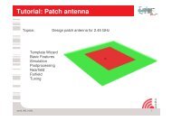
Figure 7.1. Patch array template
7.4.2 The monopole
The monopole antenna basically has the same setting as the dipole antenna. It is resonating at a quarter wave length.
Additionally, a finite ground plane can be employed in the model with the dimension to be specified in the template. This
model can be widely used for other types of antennas by specifying the ground plane size and replacing the monopole
arm with individual radiating elements.
7.4.3 Microstrip Antenna
This template will generate a very basic patch antenna on an infinite ground plane. The substrate material permittivity
(default Rogers Duroid 5880) as well as the height h (default 1524 um) are given in the initial setting. The λ 2 operating
frequency needs to be specified. The patch length and the size of the total simulation box are calculated based on these
parameters. The two switches Insert Far Field transformation and Insert field dump allows to access the near field data and
the far field data at the resonance frequency. After running the simulation the layer for the far field animation and the
layer for the field animation are activated to see the fields in the 3d mode.
7.4.4 Mobile phone
A generic model of a cellular phone is implemented to model multi band antennas in mobile devices. The Antenna height
is the distance between the upper antenna structure and the printed circuit board (PCB) and is set to 6mm by default.
With the two geometric parameters Board length (default 107mm) and Board width (40 mm), the total size of the device
can be adopted to the dimension of interest. This template is particularly useful to setup a quick simulation for any kind
of mobile devices. The position, shape and size of the Antenna structure can be rearranged and modified in order to
tackle the customer’s needs. The frequency range for this template is automatically set from 500 MHz to 2.5 GHz. And
the Farfield computation is done for 920 MHz. For this template the dimensions of the cell phone should be limited to
(C) 2006

CHAPTER 7. TEMPLATES 33
40mm < w < 100mm and 70mm < h < 150mm. The two switches model battery and model plastic casing, will generate
the phone’s battery (modeled as PEC) and a 1mm thick casing with a permittivity of 3, respectively.
7.4.5 Biquad
The BiQuad Antenna is rather simple antenna with a comparatively high directivity (about 10 dB). Each of the two
folded arms have are a wavelength (λ) long and the total structure is placed at a distance of about λ 4
over an infinite
ground plane. By entering the resonance frequency (default IMS band 2.45 GHz) the length of the two antenna arms are
calculated automatically to resonate at λ. The two switches lumped port excitation and coaxial excitation allow to define
the excitation scheme. By default, a lumped port is used to save simulation time, due to the less stringent discretization
requirements of this port type. In case of a practical BiQuad antenna a coaxial feeding line should be used.
7.4.6 Patch Antenna Array
The patch array is the most complex antenna template. By defining the patch size, as there is the length l and the width w
of the patch and the spacing (hdx and wdy) between the patches, an n x × n y array is set up. The numbers of elements n x
in x-direction and n y in y-direction are limited due to the computational resources available. An array of 10x10 Elements
and the default settings needs less than 5 minutes on a P4 architecture. The beam can be tilted by specifying the two
angles in spherical coordinates theta (θ) and phi (ϕ). Please note that for tilted beams (time delays for the ports) a correct
s-parameter evaluation is not possible. If the switch assign common port for all elements is turned off, every element will
be assigned its own port number, which allows to compute the total coupling using the n x × n y S-matrix.
7.5 Examples
Here, many examples with fixed parameters can be previewed and selected from a list. They can also be found in the
EMPIRE XCcel TM installation folder.
(C) 2006

Chapter 8
Parameter Set-up
Upon starting EMPIRE XCcel TM , most global simulation parameters have already been entered or set by an opened
project. To access and adjust these global parameters the entry Simulation Setup in the control list can be opened as shown
in Figure 8.1
Figure 8.1. Global simulation parameters
8.1 Geometry
The drawing unit determines the relation between one unit in the drawing plane and the geometry in reality. The default
is 1µm and can be changed according to the entries in the list.
34 (C) 2006

CHAPTER 8. PARAMETER SET-UP 35
8.2 Frequency
Start- and End Frequency determine the width of a Gaussian pulse which is used as the default excitation function. If the
start frequency is different from zero a modulated Gaussian pulse will be used.
Hint 11: Pulse width
It can be advantageous to excite with a pulse as short as possible to minimize simulation time.
To achieve a minimum pulse width the frequency bandwidth should be as large as possible. The end frequency determines
the maximum grid size and is limited. Therefore the start frequency should be zero to allow maximum bandwidth.
Hint 12: Start frequency
Only with a few exceptions, e.g. hollow waveguides where the minimum frequency should be above cut-off, the start
frequency should be set to 0 Hz.
The target frequency specifies the center of the frequency band where loss models are optimized for.
8.3 Prototype
In this paragraph information about the simulation problem type have to be entered.
Discretization - Algorithms can be optimized depending on information about the object types (mainly planar or
mainly 3-dimensional)
• Planar + 3D Here, the grid will be optimized for both planar and general 3D structures. The planar plane is assumed
to be xy-plane by default but can be set differently in the options menu.
• Planar Grid lines will be preferred for planar structure, i.e. one-third rule grid lines will be favored over generic
grid lines from 3D objects.
• 3D Only 3D objects will be assumed and no optimization for flat metals will be performed.
• User defined Some parameters of the automatic meshing engine in Editor options - Autodisc can be adjusted only, if
the mode is set to user defined.
• Manual This mode is used to switch off the automatic meshing engine and to define the grid manually.
Resolution - Defines the accuracy of the grid
• Coarse, e.g. 3 cells for a stripline
• Medium, e.g. 4 cells for a stripline
• Fine, e.g. 5 cells for a stripline
• Very fine, e.g. 6 cells for a stripline
Structure type - Determines number of timesteps, required energy decay and resonance estimation order depending on
typical simulation problems.
• Inductor n < 5, medium energy decay, low order estimation, e.g. single turn inductor
• Inductor n < 20, slow energy decay, low order estimation, e.g. multiple turn inductor
(C) 2006

CHAPTER 8. PARAMETER SET-UP 36
• Short Response, fast energy decay, no estimation, e.g. broad band antenna
• Medium Response, medium energy decay, high order estimation, e.g. narrow band antenna
• Filter HO slow energy decay, high order estimation, e.g. high order filter
• Filter LO medium energy decay, high order estimation, e.g. low order filter
• User Setup (Advanced) Here, the end criteria (last time step and energy decrement) and resonance estimation order
have to be defined by the user.
8.4 Simulation
By default Dielectrics and Conductors are treated as lossless. This reduces simulation time and leads to reliable results
for parameters such as reflection or coupling. In case of resonators or if the transmission losses play a significant role and
high accuracy is required the losses can be included in the simulation at different levels. Here, the frequency dependent
loss models are centered to the Target frequency which can be set in section Frequency.
Dielectrics
• lossless, ideal dielectrics
• narrow band lossy, equivalent conductivity, typically ±10% bandwidth
• medium band lossy, 1st order approximation of constant loss angle, typically ±50% bandwidth
• broad band lossy, 2nd order approximation of constant loss angle, typically ±95% bandwidth
Conductors
• lossless, ideal conductors
• narrow band lossy, constant conductivity, typically ±10% bandwidth
• medium band lossy, 1st order approximation of skin effect typically ±50% bandwidth
• broad band lossy, 2nd order approximation of skin effect, typically ±95% bandwidth
Flat metal thickness
• thin, metalization will be resolved with one gridline
• 1 cell, metalization will be resolved with two grid lines with the spacing of the conductor thickness.
8.5 Boundary conditions
These parameters determine which boundary conditions will be applied at the six sides of the simulation domain.
• Electric Tangential electric field is forced to be zero at the outermost gridline. Used for (lossless) ground planes,
metal packages, or symmetry planes
• Magnetic Tangential magnetic field is forced to be zero in the middle of the outermost cell. Used to truncate
simulation domain if both radiation and reactive field can be neglected at the boundaries. Further, can be used as
symmetry plane.
• Open n Radiating boundary condition with n Perfectly Matched Layers. The higher the number of layers the lesser
reflections will be produced at the boundary (but slows down simulation speed). The layers are placed outside the
simulation domain.
• Resistive sheet A sheet with 377Ω is placed at the boundary which absorbs radiation which is directed normal to
the boundary. Used for high directivity radiation or to suppress box mode resonances in simulations.
(C) 2006

CHAPTER 8. PARAMETER SET-UP 37
8.6 Autodisc
If not disabled, the automatic mesh generation engine will be executed each time if
• the operation Create Discretization is executed
• the button Convert and Save is used before simulation
• the button Simulation is pressed to start a simulation
• a parameter value is swept in a variation or optimization
The settings of the automatic mesh generation can be adjusted here. If the Prototype is set to User defined all parameters
can be accessed otherwise only a limited number of parameters can be changed.
The most important parameters to be adjusted will be described in chapter 14 while the complete list and description of
the different Autodisc parameters is available in chapter 19
8.7 Advanced Simulation Parameters
If item Structure Type is set to User defined the respective parameters can be set in the Advanced Display Mode.
8.7.1 Excitation
According to the entered values the shape of the pulses in frequency and time domain are displayed in the preview
windows. Also the number of frequency points used for the Frequency Transformation DFT can be adjusted.
Hint 13: Minimum number of timesteps
In the pulse preview window the required number of time steps can be estimated. At least twice the duration given in
steps have to be simulated.
8.7.2 Boundary Conditions
To enter Boundary Conditions select Boundary Conditions on the left list. Here, the boundary conditions have to be
entered by selecting the desired combination.
Figure 8.2. Boundary conditions setup
(C) 2006

CHAPTER 8. PARAMETER SET-UP 38
• Metal and magnetic boundaries can be combined with any open boundary condition
• Retarding boundary conditions (trans abs, long abs, mur) may not be combined with Perfectly Matched Layers
(pml).
• Perfectly Matched Layers (pml a) may be combined with Perfectly Matched Layers (pml b) with different numbers
of layers a,b.
Hint 14: Retarding boundary conditions
Retarding boundary conditions (trans abs, long abs) are suited for TEM like feedings (Absorbing Ports), such as Coaxial,
MSL, CPW,... The effective permittivity has to be entered and can be found in literature for many line types.
Hint 15: 1st order Mur boundary condition
First order Mur (mur) is suited for radiation problems if the radiation direction is known. if α is the angle between
radiation direction and normal vector of the boundary the effective permittivity can be obtained from ε e f f = ε r cos 2 (α)
Hint 16: Perfectly Matched Layer boundary conditions
Perfectly Matched Layers (pml) are well suited for general use. Strong reactive fields should be avoided at the boundaries.
8.7.3 End Criteria
Figure 8.3. End criteria setup
There are two possibilities to terminate the simulation run.
• Fixed number of time steps: The simulation will terminate if the value is exceeded. During the simulation this
number can be changed.
• Maximum checksum decrement: If the energy left inside the structure is declined to this value, the simulation will
be terminated.
Restarting the simulation after termination is not possible.
Hint 17: Restart
(C) 2006

CHAPTER 8. PARAMETER SET-UP 39
Remarks:
• The value for the maximum simulation time is not known in general.
• The maximum checksum decrement can be used to terminate the simulation run automatically when the energy
inside the structure is decreased below this value.
• For resonant structures simulation time can be saved using Resonance Estimation.
• The order of the averaging system gives the number of sample points which will be used for estimation.
High quality structures are able to store the energy for a long time thus causing long simulation runs for accurate determination
of results. A special resonance estimation technique can reduce simulation time drastically. A moving average
system (mAVG) is applied with an adjustable order which determines the estimation interval.
Info window:
The info window gives useful hints for the required number of time steps.
• Time step: Time step size in seconds. Depending on smallest grid size and material distribution only.
• Sample factor: Every ns time steps the signal values are stored into the time domain files, e.g ut1.
• Excitation Duration: DE, the length of the pulse in time steps
• Wave in Air: DA, approximate duration for wave traveling 1mm in free space
• Zero size structure: Calculated from DE + 2nsN, where N is the system order
• Small size structure: Calculated from 2DE + 2nsN, where N is the system order
• Minimum recommended frequency: Frequency which can be resolved by estimation. This value can be decreased by
increasing order N if the estimation interval is long enough.
8.7.4 Port Setup
Figure 8.4. Port setup
• Effective Permittivity: Has to be entered if retarding boundary conditions are applied. The value may be calculated
separately by simulating the feeding line only using PMLs. For the feed lines in the port library, an Info window
displays this value depending on the line parameters.
(C) 2006

CHAPTER 8. PARAMETER SET-UP 40
• Length of source area:
1. N = 0 for plane wave and lumped source excitation
2. N = 3 for waveguide excitation with TE- or TM-modes
3. N > 2D f /δx b for matched source excitation, where D f is the effective field diameter and δx b is the first
discretization step at the excitation boundary.
• The default value of the lumped port impedance of 50Ω which is used to separate incident and reflected waves, e.g.
ut1.inc, ut1.ref can be adjusted if the port impedance has been modified in the structure setup.
8.7.5 Cleanup Setup
The cleanup defines the files to be deleted before subsequent simulation runs.
Figure 8.5. Cleanup setup
8.7.6 Special parameters
Parameters
• Time delay in minutes: Delay for starting a batch simulation
• Oversampling factor: Determines number of timesteps written in time series files, e.g. ut1
• Parameter tolerance: Level, at which relative FDTD coefficients are treated as equal.
• Gauss attenuation at start: Level of incident pulse at timestep 0.
• Maximum Runlength: Number of Yee cells used in one system call
• Multiple Timestepping: Can be switched off if not supported by processor
• Number of Threads: Number of CPUs used for simulation
(C) 2006

CHAPTER 8. PARAMETER SET-UP 41
Figure 8.6. Miscellaneous
Switches
• Increased stability reserve: Reduces the calculated maximum time step. This can help to avoid long term instabilities.
• Excitation normalization: By default, the energy distribution of the incident pulse over the frequency is compensated
by the normalization function ef. Can be switched off.
• Wait for license: If more remote hosts are enabled than licenses available in the network this switch causes simulation
tasks to wait until licenses are checked out again.
• Save memory during set up: Memory used during compilation will be de-allocated if enabled. This may cause Out
of memory errors on 32 bit machines for large structures.
• Close Idle Processors: If enabled, only active jobs will be displayed in the batch mode.
• Speed Optimization of losses: Can be disabled to be compatible with old version
(C) 2006

Chapter 9
Object creation
This chapter gives an overview on how to create objects in EMPIRE XCcel TM . Building more complex geometries, e.g.
shaping, drilling, merging, will be described in chapter 10.
Hint 18: Object creation
New objects are created on the active layer and inherit the layer property by default.
9.1 Box
A box is defined by 6 numbers which represent two opposite points in the 3D space. In EMPIRE XCcel TM a box is mainly
used to define rectangular shapes, field dump regions, surface for far field transformations, animation planes and centers.
It can be created in the following ways.
Forward Usage
1. Press button Create Box (default)
2. Enter co-ordinate values of the box
3. Press OK
Remarks
• The co-ordinates perpendicular to the current drawing plane are defined by the layer arrow.
• Instead of entering the co-ordinate values an arrow can be drawn in the drawing area.
• Pressing the OK button can be replaced by pressing the right mouse button in the drawing area.
Backward usage
1. Draw an arrow in the drawing plane representing the box’s cross section
2. Press button Create Box (default)
Structure List
1. Select ⊞Structure ⊞Create ⊢Box
2. Enter co-ordinate values of the box
42 (C) 2006

CHAPTER 9. OBJECT CREATION 43
3. Press OK to confirm or Cancel
The structure is displayed immediately in the drawing area
Hint 19: Point input by mouse
Instead of typing the values, it is also possible to press the button Input Point by Mouse
drawing area and press left button to enter the values.
and move the cursor to the
9.2 Polygon
An N-point polygon is defined by (N+2) numbers which represent the N-point cross section and two height co-ordinates.
A polygon is closed by connecting first and last points. These objects are mainly used in planar layouts. They can be
created as follows.
Forward Usage
1. Press button Create Poly
2. Adjust extrusion arrow if necessary by pressing height=z 0.0-1000.0
3. Enter co-ordinate values of the points
4. Press OK
• Press Insert after or Insert before to add points to the polygon.
• Press Delete point
to delete a point
Remarks
• The extrusion height is defined by the layer arrow.
• Instead of entering the co-ordinate values press the button Input Point by Mouse
drawing area and press left button to enter a point.
and move the cursor to the
• Pressing the OK button can be replaced by pressing the right mouse button in the drawing area.
Backward usage
1. Enter a set of points in the drawing area
2. Press button Create Poly
Remarks
• The sequence of points entered determine which points will be connected with lines
• The last point and first point will be connected to close the polygon
• The latest entered point(s) can be deleted by pressing the Backspace key
Structure List
1. Select ⊞Structure ⊞Create ⊢Poly
2. Follow the same procedure as defined in Forward usage
(C) 2006

CHAPTER 9. OBJECT CREATION 44
9.3 Line Polygon
The special polygon Linpoly is an unclosed N-point polygon. It is a line type object and can be oriented in space by
assigning a tangential vector.
1. Enter a set of points in the drawing area
2. Press button Advanced and Create Linpoly
3. Select the line polygon
4. Switch to an alternative view
5. Enter a tangential arrow for the orientation in space
6. Press button Advanced and Set tangential
Hint 20: Line objects
Line objects are always discretized in a way that connection from first to last point can be ensured.
9.4 Bond Wire
A bond wire is a special line type object which shape is fixed by start and ending point and slope angle (third order
polynomial).
Forward usage
1. Press the icon Create Bondwire
2. Enter an arrow in the drawing area which represents the start and end point of the wire.
3. Press OK or press right mouse button
4. Adjust heights of beginning and end
5. Optionally, adjust slope angle and number of supporting points
6. Press OK or press right mouse button
Backward usage
1. Enter an arrow in the drawing area which represents the start and end point of the wire.
2. Press the icon Create Bondwire
3. Adjust heights of beginning and end
4. Optionally, adjust slope angle and number of supporting points
5. Exit by pressing Close
(C) 2006

CHAPTER 9. OBJECT CREATION 45
9.5 Circle
In EMPIRE XCcel TM a circle is a 1-point polygon with a radius > 0. Together with the height co-ordinates a circular
cylinder is defined.
Forward usage
1. Press the icon Create Circular Cylinder
2. Enter Midpoint P0 of the circle
3. Enter any point on the circumference of the circle
4. Press OK
Remarks
• The height of the cylinder is defined by the layer arrow.
• Instead of entering the co-ordinate values an arrow can be drawn in the drawing area from midpoint to any point
on the circle.
• Pressing the OK button can be replaced by pressing the right mouse button in the drawing area.
Backward usage
1. Enter an arrow in the drawing area from midpoint to any point on the circle.
2. Press the icon Create Circular Cylinder
Structure list
1. Select ⊞Structure ⊞Create ⊢Poly
2. Delete one of the points, e.g. Point 1, by pressing the Delete point button
3. Enter x and y values of the midpoint
4. Enter the radius r
5. Press OK
9.6 Segment of a circle
To obtain segments of a circle it has to be converted into a multiple point polygon first which resolution can be edited in
Editor options
1. Create a circular cylinder with method above
2. Select object, e.g. press middle mouse button
3. Press icon Merge
4. Select object at first segmentation point (green handle at P1)
5. Activate handle at second segmentation point (green handle at P2)
6. Press icon Advanced and Bisect polygon
7. Select circular segment to be deleted
8. Press Del key to erase
(C) 2006

CHAPTER 9. OBJECT CREATION 46
Remarks
• By merging a circle it will be converted to a multiple point polygon
• The number of points is determined by the circle resolution (default 11.25 degree), and can be changed in Editor
Options - Polygon - Circle Resolution
9.7 Sphere
A sphere is a special rotational polygon with the cross section of a half circle.
1. Create a half circle parallel to one axis with method above
2. Enter a 1D arrow as rotational axis (e.g. diameter of the half circle)
3. Select the circle, e.g. press middle mouse button
4. Press the icon Change to ROTPOLY
9.8 Rotational Polygon
A rotational polygon Rotpoly is defined by the polygon cross section and a rotational axis.
1. Create a (closed) polygon as described before
2. Enter a 1D arrow as rotational axis, e.g. in x-direction
3. Select the polygon, e.g. press middle mouse button
4. Press the icon Change to ROTPOLY
One example of a rotational polygon is displayed in Figure ??
Remarks
• The rotational polygon is subdivided for display. To obtain a finer resolution this number of can be changed in
Editor Options - Polygon - Rotpoly Subdivision
9.9 2D Layout Import
Imported layout objects are always represented as polygons. Layout data is often available in files which have a certain
standard. EMPIRE XCcel TM supports the following file types:
• Gerber - ending .ger, .gbr
• DXF - ending .dxf (only DXF 12)
• GDS2 - ending .gds
Before import the respective settings in the Editor options should be checked and adjusted. The most important settings
are:
• Scaling - To be adjusted if layout unit and EMPIRE XCcel TM drawing unit are different
(C) 2006

CHAPTER 9. OBJECT CREATION 47
Figure 9.1. View of rotational Polygon in the 3D mode
• Arc resolution - If Layout contain a huge amount of curved objects the import time can be reduced by enlarging the
default resolution of 5 degrees.
• Circle recognition - Automatically convert multiple point circles into single point circles to speed up drawing
• DXF connection tolerance - A value > 0 can help to join single lines into polygons.
The import procedure is executed with the following commands.
1. Select Menu File - Import - Layout and file format
2. Browse directory and select layout file
3. Select or de-select layer or additional files to be imported
4. Press Import and Close to finish the layout import
5. Browse through the layers and assign a respective height
Hint 21: Layout import
Layout files do not contain any height information and has to be set by the user. If a layer stack has been set once it can
be re-used if the layer names are identical for another layout file.
9.10 3D Solid Import
Arbitrary objects which have been generated by, e.g. a mechanical CAD tool, can be imported in STL standard (Stereo-
Lithography), a format which most of the CAD tools support.
Before import the respective settings in the Editor options should be checked and adjusted. The most important settings
are:
• Scaling - To be adjusted if drawing units are different
• Import Shift - To be set if origins are different
(C) 2006

CHAPTER 9. OBJECT CREATION 48
• Separate STL objects - In some cases several solids are grouped in one file. They can be separated if switched On
• STL Resolution - Reduce complexity of solids if less than 100% to speed up import and drawing time.
The import procedure is executed with the following commands.
1. Select Menu File - Import - 3D - Import STL object
2. Browse directory and select file with ending .stl
3. Select or de-select additional files to be imported
4. Press Import and Close to finish the import
9.11 2D Point List Import
In order to create special shapes it is possible to import a set of points from a simple list which has been created, e.g. by
another tool. After import the points will be displayed in EMPIRE XCcel TM and can be further processed, e.g. to create
a polygon with the cross section defined by the points. The points and the polygon cross section will be generated in the
current drawing plane. Therefore, the desired plane has to be selected first.
The file can have any name, e.g. list.txt and the entries have to be plain ASCII. One example of a parabolic shape could be:
0 0
100 10
200 40
300 90
400 160
600 360
800 640
1000 1000
1000 -100
0 -100
The procedure to generate this parabolic cylinder is:
1. Select Menu File - Import - User - 2D Points from File
2. Browse directory and select point list file
3. Press button Create Poly
9.12 Python Scripts
EMPIRE XCcel TM supports an interface to Python scripts which allow the generation of user defined shapes. The Python
programming language, commands and syntax is available at www.python.org.
Hint 22: Python scripts
Python scripts (ending .py) have to be located in the respective project folder.
(C) 2006

CHAPTER 9. OBJECT CREATION 49
Figure 9.2. View of rotational Polygon in the 3D mode
9.12.1 User defined polygons
To create a user defined polygon:
1. Create a layer with property, e.g. userpoly anyname $amp
2. Create a two point polygon with start and end point of the shape
One typical python script, named userdef.py to generate a user defined shape has the following content:
from math import *
def anyname (pts,args):
p2d = []
(x0,y0),(x1,y1) = pts[:2]
Amp = eval(args[0])
Include math library
function call from userpoly name in EMPIRE XCcel TM
Initializing a 2 dimensional point list
Assigning points from a 2-point polygon
Every time the drawing is updated this value is renewed
LX = int(x1-x0) Interval size
for x in range(0,LX,LX/100.):
y = Amp *(x/LX)**2
p2d.append((x+x0,y0+y))
p2d.append((x1,y0))
p2d.append((x0,y0))
Loop over x values
function with parameters
Append points to the list
Append last point
Append first point
return p2d Return point list to EMPIRE XCcel TM (C) 2006

Chapter 10
Object modification
50 (C) 2006

Chapter 11
Operations
This chapter lists a choice of operations which are often used in EMPIRE XCcel TM . A complete list of all available
operations and their explanations can be found in chapter 17.
11.1 Operators
Some operations require the input of an arrow, a point or a number. When these operators are requested in the left top
area they can be entered by either:
or
Arrow
1. Editing the values with the keyboard
2. Press OK
1. Moving the cursor to the start point of the arrow
2. Press and drag the left mouse button to the end point of the arrow
3. Press the right mouse button or OK
Point
1. Moving the cursor to the point
2. Press the right mouse button or OK
51 (C) 2006

CHAPTER 11. OPERATIONS 52
11.2 Select objects
Also it is often required to select objects. To select one or more objects several methods are available:
• Move the cursor to an object and press the middle mouse button
• Move the cursor to an object, press the Ctrl key and the left mouse button
• If objects lay on top of each other drag the mouse to toggle between objects
• Press the keys Ctrl and a to select all objects
• Press the button Select overlapping
• Press the button Select enclosed
and enter an arrow which partially or totally covers the object(s)
and enter an arrow which totally covers the object(s)
• Enter an arrow which does not touch or intersect objects to be selected and press the buttons Advanced
Select outside
and
Hint 23: Object Handles
If an object is selected the object is highlighted and small square handles are displayed on edges (boxes) or corners (polys
and soldis). The handle which is the nearest to the cursor will be activated (green square). Handles can be activated or
de-activated (red square) with the left mouse button. Multiple handles can be activated by entering an arrow covering
multiple edges of the (un-selected) object.
11.3 Move Objects
Forward usage
1. Press the button Move
2. Select objects to be shifted
3. Enter the shift arrow
Backward usage
1. Enter the shift arrow
2. Select objects to be shifted
3. Press the button Move
Mouse input
1. Select object(s) to be shifted
2. Move the mouse to one green handle
3. Press and hold the right mouse button
4. Drag the mouse to the desired position
(C) 2006

CHAPTER 11. OPERATIONS 53
11.3.1 Move Object to Layer
If objects have to be moved from one layer to another the following procedures can be applied:
1. Select object(s) to be moved to another layer
2. Open the layer list
3. Press the layer button Move selections to this layer
or
1. Open the layer list and activate the desired layer by pressing the left mouse button on the layer name
2. Select object(s) to be moved
3. Press Advanced and Move objects to the current layer
11.3.2 Parametric Move
For geometry variations it is possible to move objects parametrically. Here, the shift vector may be defined with parameters.
1. Select objects to be shifted parametrically
2. Press Advanced and Parameter Move
3. Enter shift arrow, e.g. x=xvar y=yvar and press OK
4. Enter Min Max Value Step for the parameters and press OK
Now the parameters are available in the Parameters list and the range can be verified by using the sliders.
11.3.3 Mirror Destructive
If objects should be mirrored a plane has to be defined. It is only possible to use a mirror plane which is parallel to one
of the co-ordinate axes and is defined by a 1D-arrow in the current drawing plane.
1. Switch to the desired drawing plane
2. Select objects to be mirrored
3. Press Mirror Destructive
4. Enter mirror arrow co-ordinates and press OK
• As before, instead of entering co-ordinates an arrow can be drawn and can be confirmed by pressing the left mouse
button in the drawing area.
• A 1D arrow always contains two identical co-ordinates.
• The length of the arrow can be arbitrary.
(C) 2006

CHAPTER 11. OPERATIONS 54
11.3.4 Rotate Destructive
If objects should be rotated a rotational axis has to be defined. It is only possible to use a rotational axis which is parallel
to one of the co-ordinate axes and is defined by a point in the current drawing plane.
1. Switch to the desired drawing plane
2. Select objects to be rotated
3. Press Rotate Destructive
4. Enter point co-ordinates and press OK
5. Enter rotation angle and press OK
• As before, instead of entering co-ordinates a point can be entered and confirmed with the left mouse button in the
drawing area.
• The sequence of the steps can also be mixed.
• The default rotation angle can be set in the Editor Options - Operations
11.3.5 Center
Objects can be centered to a point which can be helpful, e.g. to align objects.
1. Switch to the desired drawing plane
2. Select objects to be centered
3. Press Center to Point
4. Enter point co-ordinates and press OK
• As before, instead of entering co-ordinates a point can be entered and confirmed with the left mouse button in the
drawing area.
• The sequence of the steps can also be mixed.
11.4 Copy Objects
Hint 24: Copy Objects
Copied objects will always be generated on layers of the original objects.
Forward usage
1. Press the button Copy
2. Select objects to be copied
3. Enter the shift arrow
Backward usage
1. Enter the shift arrow
2. Select objects to be copied
(C) 2006

CHAPTER 11. OPERATIONS 55
3. Press the button Copy
Mouse input
1. Select object(s) to be copied
2. Move the mouse to one green handle
3. Press and hold the middle mouse button
4. Drag the mouse to the desired position
11.4.1 Copy to Current Layer
1. Open the layer list and activate the desired layer by pressing the left mouse button on the layer name
2. Select object(s) to be copied
3. Press Copy objects to the current layer
11.4.2 Copy Assign Arrow
The copied box gets the cross section of the entered arrow but maintains the same height as the original box
1. Select box to be copied
2. Press the button Copy Assign Arrow
3. Enter co-ordinates of the new box and press OK
• As before, instead of entering co-ordinates an arrow can be entered and confirmed with the left mouse button in the
drawing area.
• Operation available for boxes only.
11.4.3 Multiple Copy
For the generation of an array this operation is useful.
1. Select object to be multiple copied
2. Press the buttons Advanced and Multiple Copy
3. Adjust default copy expression and press OK
• The default copy expression can also be adjusted in the Editor Options - Operations
• dx, dy, dz - Shift values in x, y and z direction
• nx, ny, nz - Number of copies in x, y and z direction
• map=lambda - Mapping function for more complex arrays
Examples
dx=100,nx=9,dy=100,ny=9,dz=0,nz=0
dx=45,nx=8,map=lambda x,y,z:(100*cos(x*0.0175),100*sin(x*0.0175),0)
dx=100,nx=9,map=lambda x,y,z:(x, 0, x*x/100)
dx=0.4,nx=16,dy=0.4,ny=8,map=lambda x,y,z:(10*cos(x)*sin(y),10*sin(x)*sin(y),10*cos(y))
Comment
10x10 linear array
circular array
parabolic array
spherical array
(C) 2006

CHAPTER 11. OPERATIONS 56
Figure 11.1. Example of a multiple copy array
11.4.4 Mirror Constructive
Similar to Mirror Destructive but the original object will be maintained.
1. Switch to the desired drawing plane
2. Select objects to be mirrored
3. Press Mirror Constructive
4. Enter mirror arrow co-ordinates and press OK
11.4.5 Rotate Constructive
Similar to Rotate Destructive but the original objects will be maintained.
1. Switch to the desired drawing plane
2. Select objects to be rotated
3. Press Rotate Constructive
4. Enter point co-ordinates and press OK
5. Enter rotation angle and press OK
11.5 Stretch Objects
Forward usage
1. Press the button Stretch
2. Select objects to be stretched and press OK
3. Activate handles of corners or edges to be shifted
(C) 2006

CHAPTER 11. OPERATIONS 57
4. Enter the shift arrow and press OK
Backward usage
1. Select objects to be stretched
2. Activate handles of corners or edges to be shifted
3. Press the button Stretch
4. Enter the shift arrow and press OK
Mouse input
1. Select objects to be stretched
2. Activate handles of corners or edges to be shifted
3. Move the mouse to one green handle
4. Press and hold the right mouse button
5. Drag the mouse to the desired position
Hint 25: Stretch objects
Stretching boxes and polygons is also possible with the aid of the left list by selecting e.g. ⊞Structure ⊞Boxes ⊞L name,
press Input Coordinate by Mouse and move the cursor in the drawing area.
11.5.1 Parametric Stretch
For geometry variations it is possible to stretch objects parametrically. Here, the stretch vector may be defined with
parameters.
1. Select objects to be stretched parametrically
2. Press Advanced and Parameter Stretch
3. Enter stretch arrow, e.g. x=xvar y=yvar and press OK
4. Enter Min Max Value Step for the parameters and press OK
Now the parameters are available in the Parameters list and the range can be verified by using the sliders.
11.5.2 Scale
Objects can be scaled to their center or to the origin (green triangles on grid bar).
1. Select objects to be scaled
• Press Advanced
• Press Advanced
and Scale to Center
and Scale to Origin
2. Enter scale factor and press OK
(C) 2006

CHAPTER 11. OPERATIONS 58
11.5.3 Assign Arrow
The box gets the cross section of the entered arrow but maintains the same height as the original box.
1. Select box to be copied
2. Press the button Copy Assign Arrow
3. Enter co-ordinates of the new box and press OK
• As before, instead of entering co-ordinates an arrow can be entered and confirmed with the left mouse button in the
drawing area.
• Operation available for boxes only.
11.6 Boolean operations
In order to create more complex shapes, Boolean operations between all objects are allowed.
1. Select two or more objects to apply Boolean operations
• Merge Press the button Merge
• Subtract Press the button Subtract
• Drill Press the buttons Advanced and Drill
• Intersect Press the buttons Advanced and Intersect
(C) 2006

Chapter 12
Object properties
To all objects certain properties have to be assigned to which can be either physical or functional properties. By default
the object properties are used from the layer properties. 1
Control for all layers
• - Switch on all layers
• - Switch off all but the current layer
• - Create a new layer with default properties
• - Delete unused layers
• - Recolor all layers according to the current background color
Control for single layers
• - Move layer up in list
• - Move layer down in list
• - Switch layer on/off
• - Select layer color
• - Lock/unlock layer to prevent its objects from selection
• - Discretization modes important, basic, ignore
• - Move selected objects to this layer
• - Edit layer name or Edit property
• - Copy layer or Add property
• - Delete layer (including objects on it) or Delete Property
• - Color of fill style
• - Line width
• - Fill style
59 (C) 2006

CHAPTER 12. OBJECT PROPERTIES 60
Figure 12.1. Dielectrics data base
12.1 Basic Object Properties
12.1.1 Dielectric Assistant
Folders
• Basic - Here, the material properties can be entered manually.
• Database - A list of predefined materials can be selected for usage.
• Userbase - The user can add, modify and save his own material database.
• Info - The frequency dependence can be realized by high order Debye models and previewed in this window.
Basic
• Name - A unique name of an item in the data- and userbase or userdefined
• Rel. Permittivity - ε r ≥ 1
• Tangent Delta - tanδ ≥ 0
• Conductivity - σ ≥ 0 in 1
Ωm
• Priority Integer > 0, used for intersecting objects
Database
To use one of these materials, open one of the entries by pressing ⊞ and selecting one of the materials. Switch to Basic
to verify the selection or to Info to see the frequency dependence.
Userbase
• Folder - A unique name of an entry in the userbase list
• Name - A unique name of a material in the userbase
• Rel. Permittivity - ε r ≥ 1
• Tangent Delta - tanδ ≥ 0
(C) 2006

CHAPTER 12. OBJECT PROPERTIES 61
Figure 12.2. Conductor data base
12.1.2 Conductor Assistant
• Basic - Here, the material properties can be entered manually.
• Database - A list of predefined materials which can be selected.
• Userbase - The user may add, modify and save his own definitions
• Info - The frequency dependence of different approximation models can be previewed in this window.
Basic
• Name - A unique name of an item in the data- and userbase or userdefined
• Conductivity - σ ≥ 0 in 1
Ωm
• Thickness for skin effect - 0 < t < 10a, in µm 2
• Surface roughness - 0 ≤ R a < thickness, average roughness in µm
• Priority - Integer > 0, used for intersecting objects
• Autodisc Modeling - auto-detected or set as flat or bulk material
• Active Sides - If set to groundplane only one side is used for loss calculation.
Database
To use predefined conductors open one of the entries by pressing ⊞ and select one of the materials. Switch to Basic to
verify the selection or to Info to see the frequency dependence.
Userbase
• Folder - A unique name of an entry in the userbase list
• Name - A unique name for a material in the userbase
• Conductivity - σ ≥ 0 in 1
Ωm
(C) 2006

CHAPTER 12. OBJECT PROPERTIES 62
Figure 12.3. Lumped resistor definition
12.2 Circuit Elements
• The object type has to a box which can be flat or thin and has to be defined between two conductors
• The direction of current flow has to be specified
• Metal caps ensure a homogeneous current flow
• Lumped Resistor - Value (> 0) has to be entered in Ω.
• Lumped Capacitor - Value (> 0) has to be entered in Farad. 3
• Lumped InductorValue (> 0) has to be entered in Henry. 4
12.3 Field
12.3.1 Field storage
Only Boxes can be used to define areas of field storage.
Field distribution
Field dumps are possible for both time and frequency domain. All field nodes which are covered by the box will be
recorded. Frequency dumps are generated by an on-line DFT during the simulation run, therefore the performance can
slow down if many frequency points are used.
• Name If more than one field distribution boxes are used the names must be different.
• Domain Frequency or Time domain
• Points To specify frequencies or time steps it is possible to define equidistant sequences or single points.
• Advanced Parameters Field components can be deselected to save memory.
1 For special purposes properties can also be set directly to objects.
2 where a is the skin depth a = 1 √ (π f µσ)
3 Maximum value can be determined from N timesteps δt > 3τ = 3RC
4 Maximum value can be determined from N timesteps δt > 3τ = 3 L R
(C) 2006

CHAPTER 12. OBJECT PROPERTIES 63
Figure 12.4. Field dump definition
Nearfield to Farfield Transformation
Figure 12.5. Near-field box definition
The near-field will be recorded on each side of the entered box. Intersection of this box with material or metal boxes can
lead to unphysical results and leads to warning messages.
For scattering problems, the box should be placed outside the plane wave box to record the scattered field only.
• Name If more than one NF-to-FF boxes are used the names must be different.
• Points Only Frequency domain far field transformations are possible.
12.3.2 Field Display
The field is displayed in the 3D mode together with the structure. To hide objects their respective layers can be switched
of or set to transparent.
(C) 2006

CHAPTER 12. OBJECT PROPERTIES 64
Figure 12.6. Field animation box definition
3D Field Animation Box
Usually flat boxes are used to define planes for display of fields in 3D mode. They have to defined within the respective
field dump box and can be entered before or after the simulation.
Hint 26: Field animation plane
If only a single plane should be displayed a flat box can be defined on a single layer with both Field Distribution and 3D
Field Animation Box properties.
General
• Name of fielddump If more than one field dump has been defined, the file name has to be selected
• Frequency/Time selection - If more than one frequency has been defined for the field dump it has to be specified
here
• Normalization - Field values can be normalized for different frequency domain results, e.g. ef, if1, if1.inc
• Animation loop - Sweep over angle/timestep/frequencies or no-sweep
• Field components - E (electric field), H (magnetic field), J (current density), j (Surface current density), S (Power
flow), ACD (averaged current density), SAR (Specific Absorption Rate)
• Fielddump scaling Linear / logarithmic scaling and dynamic
• Legend keys - Switch On/Off and set number of keys for field strength vs. colors
Additional
• Arrow field Plot - Off/On/Exclusive for displaying field vectors
• Arrow Size - Length of arrows
• Line Color - On/Off and line color
• Line Type - Showing grid or lines of constant field strength
(C) 2006

CHAPTER 12. OBJECT PROPERTIES 65
Advanced
• Action - Display only or Display and Export to file after pressing the 3D button
• Weight Factor - Can be used if multiple animation boxes are used
• Field MAX value - Maximum: Automatic or absolute value
• Fielddump subsampling - Use every 1st, 2nd, 3rd, ... cell for display in the respective direction
• Fielddump move - Shift of animation display versus structure
• Fielddump type - Display style if lines are used as fill mode
• Shade Model - Interpolated or constant shading
• Fielddump fill Mode - Display styles fill, lines, points
ACD/SAR 1
• Restrict calculation - ACD/SAR can be restricted to animation box to reduce simulation time. No global maximum
can be determined in this case.
• ACD/SAR target frequency - for Gabriel parameters
• ACD/SAR cube interpolation - different standards of interpolation
• ACD/SAR max surface distance - ACD/SAR can be restricted to a certain depth of the body to reduce simulation
time.
ACD/SAR 2
• Min Number of neighbor cells - Used for tissue identification algorithms
• Tissues not zero - List of tissues found in volume
3D Farfield Animation Box
Figure 12.7. Far Field animation box definition
This box defines the center where the 3D radiation pattern is displayed in the 3D mode.
(C) 2006

CHAPTER 12. OBJECT PROPERTIES 66
Hint 27: Farfield animation center
If the NF-to-FF box can be used as the center for display a single layer with both Nearfield to Farfield Transformation and
3D Farfield Animation Box properties is sufficient.
• Filename - If more than one NF-to-FF boxes have been defined, the file name has to be selected
• Animation loop - Sweep over frequencies or phase angles, e.g. for circular polarized beams.
• Scaling - Linear / logarithmic scaling and dynamic
• Amplitude - Display relative to drawing
• Move - Shift relative to drawing
• Type - Display style if lines are used as fill mode
• Poly fill mode - Display styles fill, lines, points
• Borders - On/Off and line color for lines of constant field strength
• Legend keys - Switch On/Off legend and set number of keys for field strength vs. colors
12.4 Advanced Properties
12.4.1 Object Definition - General objects
Metal
• A metal object is defined here as a ideal conductor. Lossy metal has to be defined as material with a certain
conductivity for bulk objects or as conducting sheets.
• The default priority value for metal is higher than the default number for a material box which is used for intersecting
objects.
Material
• A material box may have homogeneous and isotropic permittivity and conductivity. The values to be entered are
the relative permittivity and the conductivity which must be given in 1
Ωm
• The default priority value for material is lower than the default number for a metal box.
Debye Material
A complex, frequency dependent permittivity can be defined using a Debye model:
Usage
• ε ∞ is the permittivity for f → ∞
• f ν are the pole frequencies
• ∆ε ν are the relative changes of permittivity
ε( f ) = ε r ( f ) − j
2π f σ( f ) = ε ∞ +
debye PRIO N EPSINF ε ∞ JUMPS [ f 1 ,∆ε 1 , f 2 ,∆ε 2 ,...]
Here, N denotes the priority number for intersecting objects.
n
∑
ν=1
∆ε ν
1 + j f
f ν
(C) 2006

CHAPTER 12. OBJECT PROPERTIES 67
Advanced Material
• The material may be an-isotropic by using, e.g [2 1 4] for the relative permittivity or permeability tensor
ε r ,µ r =
⎛
⎝ 2 0 0 1 0
0
⎞
⎠
0 0 4
• Electric conductivity, e.g. σ e = 2π f 0 ε 0 ε r tanδ
• Magnetic conductivity, e.g. σ m = 2π f 0 µ 0 µ r tanδ
• Mass density has to be defined if Specific Absorption Rate should be evaluated with mass averaging, e.g. for 1g.
12.4.2 Object Definition - Sheet objects
Sheet Resistor
• A sheet resistor in Ω can be defined
• The box must cover only one grid line in one direction.
• For the calculation of the conductivity the direction of the current has to be entered.
Sheet Resistor (Rsquare)
A direction-less square resistance can be entered if current direction is not known
Conducting Sheet
Sheet model approximation: Special algorithm for broadband modeling of skin losses.
12.4.3 Surface metalization
Surface metalization of volume objects.
• Metalization - Surface will be metalized with ideal conductor or R square resistance.
• Mask - Metalization is switched off where Mask objects intersect Metalization object.
• Unmask - Cancel Mask definition where Unmask objects intersect Metalization object.
12.4.4 Object Definition - Line objects
Line Resistor
• A line resistor with a value in Ω m
can be defined
• The object type has to be a line object, e.g. bond wire.
(C) 2006

CHAPTER 12. OBJECT PROPERTIES 68
12.4.5 Object Definition - Other objects
Voxel model
A meshed body model can be included into the simulation to evaluate the field in tissues, e.g. ACD or SAR.
• Name of the voxel file (ending .vxx), must be located in project folder
• Gabriel target frequency used for low frequency algorithm
• Fixed Permittivity if value can be neglected for simulation
• Fixed Conductivity if value can be neglected for simulation
• Store Voxel Info on / off
• Clip Region used if only part of the model is used
• Erase Start Points is used if only part of the model is used
• Anchor defines insertion point relative to voxel box co-ordinates x0, y0, z0
• Rotation limited to multiples of 90 degrees
• Length unit for display has to be set according to drawing unit
• Min Permittivity for display Tissues with lower values will be hidden
• Min Conductivity for display Tissues with lower values will be hidden
12.4.6 Measurement Definition
Voltage Box
• A voltage box fixes the integration path for the electric field.
• The voltage box has to cover exactly one grid line and has to be placed between two conducting objects 5 where the
voltage will be evaluated.
• For each port a unique number has to be defined.
Current Box
• A current box fixes the integration path for the magnetic field.
• For an outer port the current box has to be placed between the two first or two last grid lines of a boundary (It must
be placed in any case between two grid lines). The defined area has to cover the cross section of the conductor
which current should be evaluated.
• For each port a unique number has to be defined.
12.4.7 Excitation Definition
Concentrated source
• Voltage source, the structure is excited by 1 Volt.
• Impressed electric field source, the structure is excited by 1 V m
• Current source, the structure is excited by 1 Ampere.
5 an electric boundary may be regarded as an conducting object
(C) 2006

CHAPTER 12. OBJECT PROPERTIES 69
Excitation Box
• The electrical field components with the entered direction will be excited at the nodes which are covered by the
excitation box.
• The excitation box has to be defined at one of the boundaries and has to cover exactly the first or the last grid line.
• Weighting factors can be used, e.g. to double the current when using a magnetic wall.
• For each port a unique number has to be defined.
Plane Wave Excitation
Plane waves are realized as compact sources. This means that inside the box both the incident field wave as well as the
scattered field exists, whereas outside the box only the scattered field is present.
All scattering objects must lie inside the plane wave box. The scattering objects may not touch or even intersect the box.
One boundary may be chosen to be electric to simulate ground. Depending on polarization and propagation direction a
mirrored plane wave will be generated to ensure proper boundary conditions at the ground wall.
The direction of propagation is entered in spherical co-ordinates in degrees. The polarization of the wave is uniquely
defined by components of the spherical unit vectors.
More than one plane wave boxes may be defined to exploit interference effects, e.g. a standing wave to model a homogeneous
field. To calculate delay factors one plane wave has to be regarded as reference.
• E theta - θ- component of electric field for polarization in V m
• E phi - φ- component of electric field for polarization in V m
• K theta - θ- component for direction of propagation in degree
• K phi - φ- component for direction of propagation in degree
• Delay - Used for more than one plane wave excitations in s
Waveguide Port
A waveguide port can only be hollow or filled with one dielectric material. At a waveguide port more than one mode can
be taken into account by defining port numbers for every mode.
Before simulation TE and TM modes will be calculated i = 1,...,M − N + 1 They are numbered in ascending order of
their cut-off frequencies.
• Start Port Number N: N 1 > 0 6
• End Port Number M: M 1 ≥ N 1
7
• Start Excitation Port Number J: N ≤ J ≤ M
• End Excitation Port Number K: J ≤ K ≤ M
• Sign - Used to adjust phase angle at this port
• Weight - Can be adjusted to account for electric symmetry plane
Here, M − N + 1 Modes are used for termination at this waveguide port and K − J + 1 Modes are used for (subsequent)
excitations at this waveguide port.
6 nth waveguide N n > M n−1
7 nth waveguide M n ≥ N n
(C) 2006

CHAPTER 12. OBJECT PROPERTIES 70
Hint 28: Waveguide mode visualization
Modes can be visualized by
1. Adding 3D Field Animation Box to the Waveguide Box
2. Loading wg port i.dbx file
12.4.8 Other definitions
Name Object
• A name can be specified for layers or objects
• Naming convention: name anynamewithoutspaces
Poly smart discretization
For compatibility purposes only.
Ignore Object
If this property is set to a layer or object it will be ignored for simulation.
Autodisc Hints
• Autodisc Hints - important , basic , ignore or auto.
• Autodisc Modeling - treatment as flat or bulk material.
12.4.9 Experimental
Meta Material
Metamaterials are Materials with unusual and unconventional wave properties. One class of Metamaterials has a negative
refraction index (NRI). To model this NRI phenomenon, a Drude model for the electric field as well as for the magnetic
field is implemented in EMPIRE XCcel TM . For frequencies lower than the electric resonant frequency f elec and magnetic
f mag resonant frequency an effective negative permittivity ε e f f as well as a negative permeability µ e f f can be observed.
At the transition frequency the effective material parameters ε e f f and µ e f f are zero, which corresponds to an infinite
wavelength at a non-zero frequency.
µ e f f ( f ) = µ r
(
1 − f )
mag
2
f 2
ε e f f ( f ) = ε r
(1 − f elec
2 )
f 2
• Relative Permittivity - ε r positive permittivity value, which corresponds to the effective permittivity for the frequency
approaching infinity.
• Relative Permeability - µ r positive permeability value, which corresponds to the effective permeability for the frequency
approaching infinity
• Electric Conductivity - takes into account losses for the electric node in Ω m
• Magnetic Conductivity - takes into account losses for the magnetic node in Ω m
• Electric Resonance - transition frequency f elec for the electric field node
• Magnetic Resonance - transition frequency f mag for the magnetic field node
• Priority - Used for intersecting objects
(C) 2006

CHAPTER 12. OBJECT PROPERTIES 71
Diode
Nonlinear Spice Diode model. Parameters not part of Spice Model:
• Direction of the diode - only positive axes possible
• NRS: series resistance in cells - Cells for Series Resistance
• DUM: max. Voltage Step - Maximum voltage iteration step in V
• OFF: Voltage Offset - used for DC bias in small signal simulations
• SF: File to Save for LTV sim - File to save time domain diode parameters
(C) 2006

Chapter 13
Port types
The following section describes the different port types which are available in the Library Wizard. For all port types the
following hints are valid:
Hint 29: Ports
• The direction of a port must coincide with one of the major axes.
• A concentrated port may not be placed at the boundary.
• An absorbing port has to be placed at the boundary.
• The ports consist of voltage and current boxes for recording the time signals and a surface resistance with an
adjustable impedance (default 50 Ω) parallel to the voltage box.
• If the port is excited, a current source as an excitation box is added to the port parallel to the resistor.
• Its basic elements can be displayed by selecting the port and pressing the icon Explode Library Element.
Undo to recover the library element.)
(Use
To insert a port into the current drawing:
1. Select a suitable drawing plane
2. Set an appropriate layer arrow
• Press the button Open Library Wizard
• Select ⊞Ports ⊞Create
or
3. Select one of the available port types in the list 13.1
13.1 Coaxial Port
• The transverse insertion point is defined by the beginning of the height value
• The direction of the coaxial port is defined by the points Point 0 and Point 1 in the port list.
• Depending on the type of the port the reference plane (indicated by a blue line) is either at the boundary (absorbing
port) or within the structure (concentrated port)
72 (C) 2006

CHAPTER 13. PORT TYPES 73
Figure 13.1. Library Wizard: Port types
Figure 13.2. Parameters of Coaxial Port
(C) 2006

CHAPTER 13. PORT TYPES 74
1. Geometry to be entered in drawing units
• Inner Diameter, di > 0 Inner Conductor, ideal metal
• Dielectric Diameter, dd > di, Isolator
• Outer Diameter, da > dd, Outer conductor, ideal metal
2. Material
• Permittivity(rel), epsr ≥ 1
3. Priority to be adjusted if port intersects other objects
• Outer Priority, pra > 0
• Dielectric Priority, prd > pra
• Inner Priority, pri > pri
4. Concentrated Port Parameters (only for port type = concentrated)
• Ref. Impedance, R > 0 in Ω, internal load of current source
• Port Distance, pd > 0 in drawing unit, distance between load and reference plane
• Use old concentrated ports, OCP = on/o f f , no end cap is used if set to on
5. Discretization Parameters to be entered in drawing units
• Inner Disc, d0 > 0, grid spacing for inner conductor
• Dielectric Disc, d1 > 0, grid spacing for isolator
• Outer Disc, d2 > 0, grid spacing for outer conductor
• Longitudinal Disc, dL > 0, grid spacing in propagation direction
6. Advanced Parameters
• Excitation Delay, ED ≥ 0 in s, used for multiple simultaneous excitations
• Excitation weight factor, WE, used for weighting multiple ports
• Current weight factor, WC, used for, e.g. magnetic symmetry plane
• Voltage weight factor, WV , used for, e.g. electric symmetry plane
7. Start Port Definition Port at Point 0
• Start Port Type, p1t Concentrated, Absorbing, None
• Number of Start Port, p1 ≥ 1, to be adjusted for multiple ports
• Start Port Excitation p1e = On/O f f , Off - only used for termination
8. End Port Definition Port at Point 1
• End Port Type, p1t Concentrated, Absorbing, None
• Number of End Port, p1 ≥ 1, to be adjusted for multiple ports
• End Port Excitation p1e = On/O f f
13.2 Square coaxial Port
All remarks and parameters are equal to those of the circular coaxial port.
(C) 2006

CHAPTER 13. PORT TYPES 75
Figure 13.3. Parameters of Square coaxial Port
Figure 13.4. Library Wizard: Coplanar Port
13.3 Coplanar Port
• The direction of the coplanar port is defined by the points Point0 and Point1 in the port list.
• Depending on the type of the port the reference plane (indicated by a blue line) is either at the boundary (absorbing
port) or within the structure (concentrated port)
• The substrate has to be defined separately
• The port has to be defined on a layer with conductor or metal property
1. Geometry to be entered in drawing units
• Width of CPW Center Conductor, w > 0
• Width of CPW Gap, s > 0
• Width of CPW Outer Conductors, b > 0
• Met Thickness, t > 0
2. Material - ! Only used for Impedance calculation in Info Window !
• Permittivity(rel), epsr ≥ 1
3. Concentrated Port Parameters (only for port type = concentrated)
• Ref. Impedance, R > 0 in Ω, internal load of current source
• Port Load Size, pl > 0 in drawing unit, width of load in propagation direction
• Port Distance, pd > 0 in drawing unit, distance between load and reference plane
(C) 2006

CHAPTER 13. PORT TYPES 76
4. Advanced Parameters
• Excitation Delay, ED ≥ 0 in s, used for multiple simultaneous excitations
• Excitation weight factor, WE, used for weighting multiple ports
• Current weight factor, WC, used for, e.g. magnetic symmetry plane
• Voltage weight factor, WV , used for, e.g. electric symmetry plane
5. Discretization Parameters to be entered in drawing units
• Min Disc, d0 > 0, minimum grid spacing for inner conductor and gap
• Max Disc, d1 ≥ d0, maximum grid spacing for inner conductor and gap
• Longitudinal Disc, d2 > 0, grid spacing in propagation direction
• Perpendicular Height, hp > w + 2s, Minimum distance to perpendicular boundary
• Perpendicular Max Disc, d p > 0, perpendicular grid spacing
• Met Thickness Disc, dt, flat metal gird resolution
6. Start Port Definition Port at Point 0
• Start Port Type, p1t Concentrated, Absorbing, None
• Number of Start Port, p1 ≥ 1, to be adjusted for multiple ports
• Start Port Excitation p1e = On/O f f , Off - only used for termination
7. End Port Definition Port at Point 1
• End Port Type, p1t Concentrated, Absorbing, None
• Number of End Port, p1 ≥ 1, to be adjusted for multiple ports
• End Port Excitation p1e = On/O f f
13.4 Lumped Port
Figure 13.5. Parameters of Lumped Port
• The direction of the lumped port is defined by the points Point0 and Point1 in the port list.
• The lumped port may not be placed at the boundary.
(C) 2006

CHAPTER 13. PORT TYPES 77
1. Port Parameters
• Width of Port, w > 0 in drawing unit
• Port Number, p1 ≥ 1, to be adjusted for multiple ports
• Port Excitation p1e = On/O f f , Off - only used for termination
• Weight factor, WE, used for weighting multiple ports
2. Advanced Parameters
• Ref. Impedance, R > 0 in Ω, internal load of current source
• Disc, d0 > 0, grid spacing
• Excitation Delay, ED ≥ 0 in s, used for multiple simultaneous excitations
• Excitation weight factor, WE, used for weighting multiple ports
• Current weight factor, WC, used for, e.g. magnetic symmetry plane
• Voltage weight factor, WV , used for, e.g. electric symmetry plane
• Excitation Function, FE, used for multiple simultaneous excitations with different pulse shapes
• Length of metal connectors, DL ≥ 0, used if port end have to be enlarged
13.5 Perpendicular Lumped Port
Figure 13.6. Parameters of Perpendicular Lumped Port
• The direction of the perpendicular lumped port is defined by the layer arrow.
• The lumped port may not be placed at the boundary.
• The cross section of the port is defined by the Points P0 and P1.
1. Port Parameters
• Port Number, p1 ≥ 1, to be adjusted for multiple ports
• Port Excitation p1e = On/O f f , Off - only used for termination
• Weight factor, WE, used for weighting multiple ports
2. Advanced Parameters identical to usual lumped port.
(C) 2006

CHAPTER 13. PORT TYPES 78
Figure 13.7. Parameters of Microstrip Port
13.6 Microstrip Port
• The direction of the microstrip port is defined by the points Point0 and Point1 in the port list.
• Depending on the type of the port the reference plane (indicated by a blue line) is either at the boundary (absorbing
port) or within the structure (concentrated port)
• Ground metalization and substrate have to be defined separately
• The port has to be defined on a layer with conductor or metal property
1. Geometry to be entered in drawing units. If signal line is below ground plane these parameters have to entered as
negative numbers
• Width of Conductor, w > 0
• Top height, |ht| > hb + w, Minimum distance to top boundary
• Bottom height, |hb| > 0, distance between signal line and ground
• Met Thickness, |t| > 0
2. Material - ! Only used for Impedance calculation in Info Window !
• Permittivity(rel), epsr ≥ 1
3. Concentrated Port Parameters (only for port type = concentrated)
• Ref. Impedance, R > 0 in Ω, internal load of current source
• Port Distance, pd > 0 in drawing unit, distance between load and reference plane
4. Advanced Parameters
• Excitation Delay, ED ≥ 0 in s, used for multiple simultaneous excitations
• Excitation weight factor, WE, used for weighting multiple ports
• Current weight factor, WC, used for, e.g. magnetic symmetry plane
• Voltage weight factor, WV , used for, e.g. electric symmetry plane
5. Discretization Parameters to be entered in drawing units
• Min Disc, d0 > 0, minimum grid spacing for signal line
• Max Disc, d1 ≥ d0, maximum grid spacing for signal line
• Transverse Disc Width, wd > 0, minimum distance to transverse boundary
(C) 2006

CHAPTER 13. PORT TYPES 79
• Perpendicular Disc, d p0 > 0, minimum perpendicular grid spacing
• Perpendicular Max Disc, d p > 0, maximum perpendicular grid spacing between signal and ground
• Perpendicular Big Disc, d p > 0, perpendicular grid spacing to boundary
• Longitudinal Disc, d2 > 0, grid spacing in propagation direction
• Met Thickness Disc, dt, flat metal gird resolution
6. Start Port Definition Port at Point 0
• Start Port Type, p1t Concentrated, Absorbing, None
• Number of Start Port, p1 ≥ 1, to be adjusted for multiple ports
• Start Port Excitation p1e = On/O f f , Off - only used for termination
7. End Port Definition Port at Point 1
• End Port Type, p1t Concentrated, Absorbing, None
• Number of End Port, p1 ≥ 1, to be adjusted for multiple ports
• End Port Excitation p1e = On/O f f
13.7 Stripline Port
Figure 13.8. Parameters of Stripline Port
• The direction of the stripline is defined by the points Point0 and Point1 in the port list.
• Depending on the type of the port the reference plane (indicated by a blue line) is either at the boundary (absorbing
port) or within the structure (concentrated port)
• Ground metalization and substrate have to be defined separately
• The port has to be defined on a layer with conductor or metal property
1. Geometry to be entered in drawing units.
• Width of Conductor, w > 0
• Top height, ht > 0, Distance to top ground
• Bottom height, hb > 0, Distance to bottom ground
• Met Thickness, t > 0
2. Material - ! Only used for Impedance calculation in Info Window !
(C) 2006

CHAPTER 13. PORT TYPES 80
• Permittivity(rel), epsr ≥ 1
3. Concentrated Port Parameters (only for port type = concentrated)
• Ref. Impedance, R > 0 in Ω, internal load of current source
• Port Distance, pd > 0 in drawing unit, distance between load and reference plane
4. Advanced Parameters
• Excitation Delay, ED ≥ 0 in s, used for multiple simultaneous excitations
• Excitation weight factor, WE, used for weighting multiple ports
• Current weight factor, WC, used for, e.g. magnetic symmetry plane
• Voltage weight factor, WV , used for, e.g. electric symmetry plane
5. Discretization Parameters to be entered in drawing units
• Min Disc, d0 > 0, minimum grid spacing for signal line
• Max Disc, d1 ≥ d0, maximum grid spacing for signal line
• Transverse Disc Width, wd > 0, minimum distance to transverse boundary
• Perpendicular Disc, d p0 > 0, minimum perpendicular grid spacing
• Perpendicular Max Disc, d p > 0, maximum perpendicular grid spacing between signal and ground
• Perpendicular Big Disc, d p > 0, perpendicular grid spacing to boundary
• Longitudinal Disc, d2 > 0, grid spacing in propagation direction
• Met Thickness Disc, dt, flat metal gird resolution
6. Start Port Definition Port at Point 0
• Start Port Type, p1t Concentrated, Absorbing, None
• Number of Start Port, p1 ≥ 1, to be adjusted for multiple ports
• Start Port Excitation p1e = On/O f f , Off - only used for termination
7. End Port Definition Port at Point 1
• End Port Type, p1t Concentrated, Absorbing, None
• Number of End Port, p1 ≥ 1, to be adjusted for multiple ports
• End Port Excitation p1e = On/O f f
(C) 2006

Chapter 14
Discretization
14.1 Automatic Discretization
Figure 14.1. General Adjustments
The automatic discretization creates a suitable mesh for the entered structure. It should be used after all structure and
excitation information has been entered.
Hint 30: Grid statistics
81 (C) 2006

CHAPTER 14. DISCRETIZATION 82
Information about the current discretization can be obtained by
• Pressing the right mouse button on one of the grid bars, Figure 14.2
• Open the left list ⊞Advanced ⊞ Discretization
Figure 14.2. Bottom grid bar
Depending on the structure only a few parameters have to be adjusted in Simulation Setup - Autodisc :
14.1.1 General
• Relative Drawing accuracy This number times the boundary distance gives the absolute drawing accuracy in each
direction. Below this threshold co-ordinates will be treated as identical.
• Relative Limit for warning A warning message will be displayed if grid spacing is below this number times the
boundary distance in each direction.
14.1.2 Directions
x,y,z-discretization in units
• off The automatic discretization is turned of in this direction.
• auto Automatic discretization will be used.
• auto+fixed As auto but fixed lines (black and bold) will be kept.
• number Equidistant mesh with a spacing of selected number.
14.1.3 Simulation Box
In some cases additional space to the boundaries will be required which can not be detected from the automatic meshing
routines, e.g. if coils or antennas with a large reactive volume should be simulated.
In other cases the simulation domain should be truncated to model only a part of the structure, e.g. for large circuits
where far distance components can be neglected.
Simulation Box X,Y,Z
• The numbers displayed in min and max are the current boundary positions
• By pressing from structure all objects will be evaluated and a overall bounding box defines the boundary.
• To adjust the simulation box by hand the co-ordinates can be edited.
• By pressing Apply the displayed values will be used for boundaries.
(C) 2006

CHAPTER 14. DISCRETIZATION 83
14.1.4 Resolution
Values can only be modified if Simulation Setup - Prototype - Discretization is set to User defined.
• Min Cells per Wavelength The minimum number of cells per wavelength may not be smaller than 5. Recommended
10. High precision 20.
• Absolute min resolution in units Co-ordinates below these numbers will be treated as equal.
• Min. Resolution in units Minimum cell spacing
• Max. Resolution in units Maximum cell spacing, if set to None it will be determined from maximum frequency.
• Object cells Number of cells used to resolve box-type objects
• Refinement ratio Used to generate a graded mesh between small and large cells.
14.1.5 Options
Values can only be modified if Simulation Setup - Prototype - Discretization is set to User defined.
• Planar Direction Default value is z (xy-plane). Can be changed if needed.
• Arc Resolution Angular step to discretize circles and arcs.
• Flat metal recognition limit This factor is used to decide if metal is treated as flat.
14.1.6 Layers
Discretization hints can also be given for each layer separately by switching the button
• Objects on this layer are important for grid generation, e.g. signal lines, hot vias, ports, etc.
• Objects on this layer don’t need accurate grid resolution, e.g. via fences, ground planes, etc.
• Ignore objects of this layer for grid generation, e.g. field dump boxes, labels, etc.
14.2 Manual Discretization
The Manual Discretization can be enabled by
• Setting Simulation Setup - Prototype - Discretization to Manual
• Press the left mouse button on one of the grid bars and confirming dialog boxes
• Loading an old input file, ending .gym, which has been generated with Empire v4.20 or older
14.2.1 Generic discretization
Press left mouse button on one of the grid bars:
• Deletes initial grid and inserts fixed lines on object edges
• Deletes initial grid and inserts a graded mesh between every pair of fixed lines
• In marked intervals inserts a graded mesh between a pair of fixed lines
• Deletes initial grid and generates a mesh using Generic Disc and Smoothing Algorithms using a maximum
grid spacing of the entered number
(C) 2006

CHAPTER 14. DISCRETIZATION 84
14.2.2 Delete Lines
Press left mouse button on one of the grid bars:
• Press the middle mouse button on one line in the grid bar
• Delete the whole grid lines
• Delete only un-fixed (red) grid lines
• Delete range defined by entered arrow
• Delete range (only un-fixed lines) defined by arrow
• Delete grid line defined by entered point
14.2.3 Add lines
Press left mouse button on one of the grid bars:
• Press the middle mouse button on empty space of the grid bar
• Add fixed lines defined by points or tips or arrows
• Add un-fixed lines defined by points or tips of arrows
• Add grid lines in the marked interval with the spacing of δ
• Add grid lines in the marked interval with n equal subdivisions
14.2.4 Port discretization
• Select Port
Delete initial mesh and insert grid proposed by the port
• Select Port, select grid bar
• Select Port, select grid bar
Add grid proposed by the port
Add local grid proposed by the port
(C) 2006

Chapter 15
Simulation
After the structure has been set up the input data has to be converted into a suitable format (file with ending .acad) to be
further processed by the EMPIRE XCcel TM kernel. This is done by
• Pressing Convert & Save
• Pressing Start Simulation
generate the .acad file and display input statistics
to generate the .acad file and start a basic simulation directly.
Hint 31: Project folder
It is recommended to use one working directory for every project. All simulation data will be stored within or beneath
this directory path. The input file has the ending .gym and contains all necessary information for the simulation. Use Save
as to generate copies of the project.
15.1 Basic Simulation
The simulation will be started by pressing the Start Simulation button . In the upper left region of the EMPIRE XCcel TM
window the progress of compilation is being displayed. The simulation starts when the display mode is switched to
Voltage where the evolution of the time domain signals is depicted. The simulation is finished when the display mode is
switched to S-Parameters. The simulation can be aborted by pressing the button.
In case of multiple port excitations, the next port will be excited and a new simulation will be started automatically.
15.2 Advanced Simulation
If more details of the simulation should be displayed the user can switch to the Advanced display mode after pressing the
button Convert & Save .
The simulation is started by selecting Processing - Start in the list and pressing the button Complete Simulation. Then
a log window is displayed, as in Figure 15.1, where some internal information like warnings, messages, and errors are
displayed. During the simulation run, performance and status of the simulation are displayed in the monitor part and
checksums are given to estimate the remaining energy inside the structure.
Setup
• Output level Displays more or less output in the log window
• Number of Timesteps Can be adjusted during simulation
• Checksum Decrement Can be adjusted during simulation
• Apply Set new values
85 (C) 2006

CHAPTER 15. SIMULATION 86
Figure 15.1. Snapshot of a running job
Admin
Action
Status
• Clear Clear log windows
• Save log Save log window to file
• Close Close log window and return to section Processing - Start
• Start Page Return to section Processing - Start without closing log window
• Kill Terminate current simulation without result generation
• Output Sync Write out current near field data
• Steps Already simulated time steps
• Performance measured in million cells each second
• Checksum E,H current checksum decrement, which is a measure for energy, for E and H fields
• Time Time needed to reach the number of time steps
It is possible to adjust the number of time steps during the simulation. This can be useful if the time signals have reached
steady state long before the simulation ends, or if the signals don’t decay fast enough so a larger number of time steps
should be given. The expected end time is displayed in the monitor part of job control. For multi-port simulation, this
time refers to the current port only.
Hint 32: Intermediate results
To obtain intermediate frequency domain results, a new job can be started by returning to the Processing - Start section
and pressing the button PostProc. DFT’s of the current time signals will be performed and the scattering parameters will
be calculated.
(C) 2006

CHAPTER 15. SIMULATION 87
15.3 Batch processing
If several jobs should be executed after another a batch control can be used for this task. For all jobs which should be
simulated the converted files .acad have to exist in the respective folders. To select the different jobs, the search path and
the search depth have to be selected. The jobs to be executed can then be selected by checkmarks.
Figure 15.2. Batch control window
Batch Control
Press Add to add one or more batch jobs to the list
Batch Start
• Simulation Start batch processing
• Postprocessing Generate intermediate results
Batch Admin
• Delete Batch Close batch control
• Close Idle Close finished batch jobs
• Kill All Terminate batch processing - no results will be generated
Batch Setup - Files
• Batch Root relative to current project folder, e.g. .. parent folder
• Search Depth relative to batch root, e.g. 2 for parent folder
• Delete all listed folders (!)
• Generate new subfolders
• Select New Select all new jobs
(C) 2006

CHAPTER 15. SIMULATION 88
• Select All Select all jobs
• Deselect All Deselect all jobs
• Refresh Start new job search
• Stop Filesearch Terminate job search
Batch Setup - Hosts
• Single host - Enable localhost
• Multiple hosts - See section Remote processing
15.4 Optimization
If parametric objects or parametric values have been defined , they can be be varied or optimized using the variator or
Discrete Gradient, respectively. The variator simulates all parameter combinations subsequently. The Discrete Gradient
applies a certain strategy to find the optimum parameter set following the entered optimization goal and terminates the
process if the goal has been reached.
Figure 15.3. Optimizer control window
Control
• Optimization - Press button Add Optimization to add one or more optimization controls
• Optimization Options - The Log Level determines the amount of log output
• Subdirectory Selection - Used only for sequential optimizations
Optimization Action
• Start - Start optimization process
• Stop - Stop optimization process
• Postprocessing - Generate intermediate results
• Clear Log - Empty log window
(C) 2006

CHAPTER 15. SIMULATION 89
• Save Log - Save log into a file
• Delete - Close Optimization control
• Close Idle - Close finished simulations
• Delete Subdirs - Delete previous results
Setup - General
• Optimizer - Optimization method
• Initial Step Factor - Step enlargement for first iteration
• Step Factor Decay - Step decay for next iteration
• Sequential Subdir Calculation - Used for result dependent optimization
Setup - Goal
• Source Files - To be used for goal definition. Press >>> to add to Terms window.
• Parameter Min - Start value of target interval, e.g. f 1
• Parameter Max - End value of target interval, e.g. f 2
• Equation - Goal function. Press >>> to ad to Terms window.
• Reference - Reference Value used for error function.
• Weight - Value used to weight different goals.
Figure 15.4. Goal definition for optimization
Setup - Hosts
• Single host - Enable localhost
• Multiple hosts - See section Remote processing
Setup - Log Window displaying current error and progress of optimization.
(C) 2006

CHAPTER 15. SIMULATION 90
15.5 Remote Processing
If multiple licenses are available in a network, the jobs in the batch and optimization control can be executed remotely
on every machine on which EMPIRE XCcel TM is installed and the empire-server is running on. This works for Linux and
Windows and cross installations.
Figure 15.5. Hosts control window
• Add Processor - Select specific host or processor to the host list
• Update Status - Refresh list of available host
• Get hosts - Get a list of all available hosts in the LAN
• Host - Name of the processor to be added to hostlist
• Process Number limit - Specify number of jobs which can be handled by this processor in parallel.
• - Delete host from list
• - Select host for processing
• State - busy if host is processing an own job
• Host - Hostname in network
• Job Limit - Number of jobs which can be run simultaneously
• Availability - Yes / No
• Performance - in Mcells/s
(C) 2006

CHAPTER 15. SIMULATION 91
• Admin - Information of owner, RAM size, etc.
• Jobs - Number of currently running jobs on this host
• Users - Owners of currently running jobs
(C) 2006

Chapter 16
Results
After the simulation all desired values like S-parameters or field dumps are available to be displayed or further processed
by special tools described in this chapter.
16.1 Graph display set up
The following graph display modes are available:
1. Voltage: Voltage time signals files are detected and displayed linear
2. S-Parameters: S-parameter files are detected and displayed logarithmic
3. Impedance: Impedance files are detected and displayed with real and imaginary parts
4. Farfield: Radiation patterns are detected and displayed
5. Additional: User defined graph set up
All setups can be can be changed and saved for the current project.
16.1.1 Display
Graph
Display of the results depending on the adjustments in the Setup. Labels and graph style can be changed in Options.
Legend
Colors and names of the graphs which are displayed, which can be switched on/off
Actions
• update - Reread current data base and update the graph
• print - Print graph
• separate - Open the graph display in a separate window
• save - Save current settings selected in setup and options
• save zoom - Save current zoom selection
• autoscale - Reset zoom
• copy - Copy graph to the windows clipboard to be used, e.g. in Office tools
92 (C) 2006

CHAPTER 16. RESULTS 93
• zoom - Zoom is done by dragging a rectangle in the graph window. Pressing this button displays a help text in the
status area.
• marker - Markers are activated by selecting one of the graphs with the cursor. Pressing this button displays a help
text in the status area.
Status
Displays xy values depending on the cursor position in the graph or a help text after pressing a button.
16.1.2 Setup
General selection - Type
• u(t) - voltage in time steps
• i(t) - current in time steps
• u(f) - voltage over frequency
• i(f) - current over frequency
• s(f) - S-parameters in a Cartesian grid
• s(f) Smith Chart - S-parameters in a Smith chart display
• s(f) Polar - S-parameters in a polar diagram
• z(f) - impedance over frequency
• y(f) - admittance over frequency (to be enabled in Advanced - Postprocessing - General Setup)
• p(f)- power over frequency (to be enabled in Advanced - Postprocessing - General Setup)
• e() - Farfield over angle in a Cartesian grid (to be enabled in Advanced - Postprocessing - Farfield)
• e() polar - Farfield in a polar diagram (to be enabled in Advanced - Postprocessing - Farfield)
• e,h path - Electric or magnetic field along a path (to be enabled in Advanced - Postprocessing - Equations
• sc(f) - Scattering cross section over frequency Advanced - Postprocessing - Farfield - Frequency dependent results)
General selection - Flavor
• magnitude lin = |y(x)| Magnitude in linear style
• magnitude dB = 20log|y(x)| Magnitude in logarithmic style
• angle degrees = ϕ( f ) = 180
π
• group delay = 1
• VSWR = | 1+s
1−s |
dϕ
2π d f
arctan
Is
Rs
• magnitude lin/angle - Linear magnitude and angle in degree of complex value
• magnitude dB/angle - Logarithmic magnitude and angle in degree of complex value
• Re/Im - Real and imaginary part of complex value
• Re - Real part of complex value
(C) 2006

CHAPTER 16. RESULTS 94
• Im - Imaginary part of complex value
General selection - Name in Legend
Usage
• - Folder and filename, where project folder is regarded as root folder
• - Filename, only
• anyname - Name can be userdefined
1. Select or enter Name in legend
2. Select file in Files list
3. Press add ==> (or right mouse button) to add to Graphs list
General selection - File Filter
The Files list detects result files automatically depending on the Type selection. It may contain many files, especially in
parameter variation subfolders. The automatic file detection can be limited by applying a file filter.
Usage
1. Enter a filter expression using the wildcard replacer *, e.g. ut*
2. Press reread in the Action area
Scaling
The range of the graphs can be adjusted by selecting one of the predefined values or by entering values manually. The
values have always to be entered in basic units, e.g. in Hz for the frequency (1 GHz = 1000000000 = 1e9).
Curves
• xstart - Left limit of graph
• xstop - Right limit of graph
• xgrid - Interval size of grid lines on ordinate
• ystart - Bottom limit of graph
• ystop - Top limit of graph
• ygrid - Interval size of grid lines
Files - List of result files which are detected automatically depending on the Type selection.
Graphs - List of result files which are selected for display.
Action
• add ==> - Add result file from Files to Graphs list
• import - Add result file from other projects to the Files list. This is very helpful for displaying results from different
simulation runs or measurements.
• delete - Delete result file from the Graphs list
• delete all - Clear Graphs list
• view - Switch back to Display using the current selections
• reread - Update Files list
• save - Save settings for the selected display mode
• export - Generate a .gif image of the graph
(C) 2006

CHAPTER 16. RESULTS 95
16.1.3 Options
General
• Title - Can be selected from a list (e.g time, date, project folder) or userdefined
• Xlabel - Can be selected from a list or userdefined
• Ylabel - Can be selected from a list or userdefined
• Xaxis unit prefix - Scaling factor for x axis
• Yaxis unit prefix - Scaling factor for y axis
• Legend position - Used for exported images
• Max. file search depth - Autodetection of result files for the Files list. Default is 1.
• Display time axis - If enabled the number of time steps is multiplied by time step size
• Use symbols - Can be used to distinguish curves if colors are insufficient
Screen
Properties of the screen display
• Maximum Number of Data points
• Geometry
• Automatic Update
• Use big crosshair cursor
• Legend in separate window
Export
Properties of the export images
• Maximum Number of Data points
• Format Computer Graphics Meta-file format .cgm output is well suited to be imported in e.g. Word documents and
can be further processed.
• Font Size of characters
• Resolution
• Export color plot black/white or colored lines
• Use dashed lines Dashed lines can be selected for a black/white output
• Landscape output or portrait style
Print
Only used for Linux operation systems. On Windows, the usual printer menu is used.
Smith Chart, Polar
• Char. Impedance - Smith Chart (SC) impedance
• Number of tics - SC Number of internal impedance circles
(C) 2006

CHAPTER 16. RESULTS 96
• Polar Number of angle tics - Number of angle intervals
• Polar Number of radius tics - Number of radius intervals
• Tic factor - SC factor between impedance circles
• Start frequency - SC first frequency to be displayed
• Stop frequency - SC last frequency to be displayed
• Frequency steps - SC Number of steps between Start and Stop frequency
16.2 Advanced Postprocessing
To obtain more advanced results already calculated data can be further processed. This is done in the Advanced display
mode in section Postprocessing
Hint 33: Advanced display mode
The Advanced folder can only be opened if the Convert and Save button
carried out.
has been pressed or a simulation has been
An overview of the subfolder structure and the available data is gathered in the subfolder list.
16.2.1 List of Subfolders
Here, the definitions of the results are displayed by pressing ⊞
sub-i (i is a number of a port which has been excited)
• DFT Definition of frequency transformations
• FDTD Time domain results
• INCREF Calculation of incident and reflected waves 1
• P Available if enabled in General setup
• SPAR Calculation of S-parameters
• USERDEF Userdefined equations
• Z Impedance calculation definition
• Y Available if enabled in General setup
sub-all Result folder for all subdirectories
• USERDEF Userdefined equations
spar Result folder for all S-parameters
• USERDEF Location for S-parameter source files only, e.g. Touchstone files
ypar Result folder for all Y-parameters
• USERDEF Location for S-parameter source files only, e.g. Touchstone files or Spice net lists.
The Delete Selection applies to the USERDEF folders only.
1 lpi is the lumped port impedance
(C) 2006

CHAPTER 16. RESULTS 97
16.2.2 General Setup
Hint 34: Advanced settings
If settings have to be changed or equations have been entered for Postprocessing use the Save button
settings.
to store the
• Power Calculation To be enabled if power of ports shall be calculated
• Admittance Calculation To be enabled if admittance of ports shall be calculated
• Update Update the subfolder list
• Reset Close the subfolder list
16.2.3 Equations
Hint 35: Userdefined equations
Equations can be defined by
1. pressing on one of the USERDEF folders
2. selecting a suitable equation type
3. editing the equation
Time/Frequency domain
Linear Equation
y(t, f ) = a 1 x 1 (t, f ) + a 2 x 2 (t, f ) + ...
Usage
1. press on USERDEF in the desired subfolder sub-i
2. press on Linear equation
3. Enter destination file name
4. Enter factor a 1 and select result file
5. Optionally, press Add button to add more terms
File Copy
y(t, f ) = f olderexpression\x(t)
Usage
1. press on USERDEF in the desired subfolder sub-i
2. press on File Copy
3. Enter destination file name
4. Enter copy expression, e.g. ut3 = ..\\sub − 3\ut1
(C) 2006

CHAPTER 16. RESULTS 98
Frequency Domain
Voltage/Current Processing - Relation
y( f ) = x 1 ( f )/x 2 ( f )
Usage
1. press on USERDEF in the desired subfolder sub-i
2. press on Relation
3. Destination Enter destination file name
4. Terms Enter (complex) frequency domain result files
Voltage/Current Processing - Symbolic Equation
y( f ) = y 1 (x 1 ( f )) + y 2 (x 2 ( f )) + ...
Usage
1. press on USERDEF in the desired subfolder sub-i
2. press on Symbolic equation
3. Enter destination file name
4. Enter source file x 1
5. Optionally, press Add button to add more source files
6. Enter mathematical expression Term
S-Parameter Processing - Loss Calculation
If N is the number of ports:
√
s 0 i = 1 − ∑ N n=1 |s n i| 2
Usage
1. press on USERDEF in the desired subfolder sub-i
2. press on Loss calculation
3. Select Loss Calculation S-Parameters
S-Parameter Processing - Touchstone File
f ile.snp = Touchstone(n × n -S-Matrix)
Usage
1. press on USERDEF in the subfolder spar 2
2. press on Touchstone File
3. Destination Filename
4. Select S Parameter Ports
Y-Parameter Processing - Y and S parameter
f ile.snp = Y PAR(n × n-Y-Matrix)
Usage
2 or ypar if enabled
(C) 2006

CHAPTER 16. RESULTS 99
1. press on USERDEF in the subfolder ypar
2. press on Y and S parameter
3. Destination Filename
4. Select Y/S Parameter Ports
Y-Parameter Processing - Y and S parameter for deembedding
f ile.snp = Y PAR DEEM(n × n-Y-Matrix)
Usage
1. press on USERDEF in the subfolder ypar
2. press on Y and S parameter for deembedding
3. Destination Filename
4. Select Y/S Parameter Ports
Y-Parameter Processing - Spice Model
f ile.net = Y PAR(n × n-Y-Matrix)
Usage
1. press on USERDEF in the subfolder ypar
2. press on Spice Model
3. Destination Filename
4. Select Spice Parameter Ports
• Destination Filename - ending .net
• Spice Parameter Ports - Convention: every odd port i is connected to the even port i+1
• Frequencies Frequency range for fitting spice model
16.2.4 Farfield
This setup is only available if an NF-2-FF box has been defined in the simulation set up and a file called, e.g. nf2ff 1 has
been generated.
Usage To add a Farfield equation
1. Select the subfolder where the far field has to be calculated, e.g. sub-1
2. Press on USERDEF in the subfolder list
3. Press on Far Field Calculation
Farfield Setup
• Near field file - File name which has been used in the NF-to-FF property definition
• Normalization - Select between Directivity, Excitation, Gain, or Maximum
• Sweep Mode - Single angle sweep or sweep over both angles
• Fixed Angle - in degree, for single angle sweep
(C) 2006

CHAPTER 16. RESULTS 100
• Angle Step - in degree, for angle to be swept
• Angle Start - in degree, for angle to be swept
• Angle Stop - in degree, for angle to be swept
• Rotation - used to swap radiation direction to z-axis
• Phase Center Translation - in m, e.g. z 1e − 3 for 1 mm
• Array Setup - linear or rotational array
Selection
• General - Enable transformation - Can be disabled to save time in subsequent postprocessings
• General - Frequency dependent results - Used to generate, e.g. gain vs frequency
• Frequency in Hz - List of frequencies defined in the NF-to-FF property definition
• Output - To select the desired Farfield components
• Misc - RCS calculation - Scattering cross section calculation
• Misc - Power calculation - determined from Poynting vector integration on NF-to-FF box
• Recognize near field at - Can be disabled if radiation in the respective direction can be neglected
• Enable BOUNDARY Mirroring at - To be used if a symmetry plane has been used
• FF BOX Mirroring at - can be used if a symmetry plane should be defined at one side of the NF-to-FF box
16.2.5 Field Path
This setup is only available if a dump box has been defined in the simulation set up and a file called, e.g. fdump 1 has
been generated.
Field Path Setup
• Field Distribution File Name of the field dump defined in structure setup
• Output File Prefix Can be selected to distinguish different result files
• Normalization - Can be normed to 1A if1, 1V uf1, or excitation function ef for absolute value
• Factor weight
• Samples Number of supporting points used in field path
Points (Units)
Points have to inside the respective field dump box.
Usage
1. X Enter x coordinate of start point
2. Y Enter y coordinate of start point
3. Z Enter z coordinate of start point
4. Add Add subsequent points to define a path through the field dump box
5. Delete Delete last entered point
(C) 2006

CHAPTER 16. RESULTS 101
Selection
• General - Calculation can be disabled to save time in subsequent postprocessings
• Frequency in Hz - Frequency points which have been defined in field dump definition
• Output - Select component
• Interpolation - Select or deselect interpolation schemes
(C) 2006

Part III
User Interface Reference
102 (C) 2006

Chapter 17
Actions
17.1 Clear
1 Clear Selections
Shortcut: Esc
All selections will be de-selected.
Pressing this button will clear all stack entries.
Equivalent to ESCAPE key.
17.2 Copy
2 Copy
Operates on Polygon Objects, Solid Objects, Box Objects,operand Arrow Objects.
Shortcut:
Copy selected OBJECT(s) according to the entered ARROW(s).
Selection: OBJECT and ARROW
3 Mirror Constructive
Operates on Polygon Objects, Discretisation Objects, Solid Objects, Box Objects,operand Arrow Objects.
Shortcut:
103 (C) 2006

CHAPTER 17. ACTIONS 104
The selected OBJECTs/GRID lines are mirrored at a 1D ARROW.
The selected OBJECTs/GRID lines are maintained.
Note:
Only 1D arrows are permitted for mirror operation.
Selection: OBJECT/GRID lines and ARROW
4 Copy Assign Arrow
Operates on Box Objects,operand Arrow Objects.
Shortcut:
Creates new BOX(es) with the cross section of the entered ARROW(s).
The height is copied from the selected BOX.
Selection: BOX and ARROW(s)
5 Rotate Constructive
Operates on Polygon Objects, Solid Objects, Box Objects,operand Point Objects.
The selected OBJECTs will be rotated around the
entered POINT which acts as the rotational axis.
The rotation angle is entered positive for counterclockwise
rotation.
Original objects are maintained.
Note:
Angle may be parametric, e.g. a
17.3 Create
6 Create Box (default)
Operates on Arrow Objects.
Creates a BOX from an ARROW.
Forward usage:
- Press Button
- Enter BOX co-ordinates on the left / Enter Arrow
- Press OK
Backward usage:
- Enter an arrow in drawing area (drag left mouse button)
- Press Icon
Note:
The layer height has to be normal to the current view.
(C) 2006

CHAPTER 17. ACTIONS 105
7 Create Cylinder (default Circular)
Operates on Arrow Objects.
Creates a 3D circular cylinder defined by an arrow.
The starting point of the ARROW is the origin of the circle
and the length defines its radius.
Forward usage:
- Press Button
- Enter co-ordinates on the left / Enter an arrow
- Press OK
Backward usage:
- Enter an arrow in drawing area (drag left mouse button)
- Press Icon
Note: The layer height must be normal to the current view.
8 Create Poly
Operates on Point Objects.
Creates a closed POLYgon from a set of POINTS.
Forward usage:
- Press Button
- Enter Point co-ordinates on the left
- optionally, insert points by pressing up/down icons
Backward usage:
- Enter set of points in drawing area (left mouse button)
- Press Icon
Note: The layer height has to be normal to the current view
Note: Each corner can be rounded by
- Open the left list + Structure + Poly
- Select desired Poly
- Enter radius value of each corner
9 Create Bond Wire
Operates on Arrow Objects.
Create a bond wire between the start and end
point of the entered arrow.
The height and slope information is entered afterwards
or can be adjusted in the options menu: Bond wires.
A third-order polynomial will be used as the shape.
10 Insert Port
(C) 2006

CHAPTER 17. ACTIONS 106
Starts the Library wizard for port definition
Inserts a (parallel) PORT into the structure which
- has the direction of a 1D arrow between Point 0 and Point 1
- insertion height is defined by the current layer arrow
Exception:
Perpendicular (lumped) Port
- has the direction of the current layer arrow
- cross section is defined by Point 0 and Point 1
Note:
MSL, CPW and Stripline Ports get the properties of the current layer.
Coaxial and Lumped Ports possess their own properties.
11 Create Discretisation
Starts the Automatic Meshing Engine, to e.g. check the structure
after discretization.
Depending on the entered objects, layer settings, and global
parameters in the Simulation Setup a grid is generated automatically.
This operation is also executed on pressing "Convert and Save" or
"Start simulation" unless the Discretization is set to "Manual".
The Autodisc Parameters may be adjusted in the Simulation Setup.
Advanced Autodisc parameters may only be adjusted if the
Discretisation is set to "User-defined"
17.4 DRC
12 Discretize
The structure is discretized using the current grid and
displayed in the 3D rendered mode. To return to the
drawing mode, press ’Draft’ Display.
The original strucutre will not be modified.
Note: Recommended for checking staircase approximation.
17.5 Delete
13 Empty Discretisation
Operates on Discretisation Objects.
Deletes all non-fixed lines on the selected GRID bar.
Non-fixed Lines are thin and red.
Note:
To de-select a GRID bar, press ESC.
14 Empty Fixed
(C) 2006

CHAPTER 17. ACTIONS 107
Operates on Discretisation Objects.
Deletes all lines (fixed and non-fixed) on the selected GRID bar.
Note:
To de-select a GRID bar, press ESC.
Undo will work.
17.6 Display
15 Zoom Extends
Shortcut: z
Displays the drawing to the overall extends.
Note:
Zoom may influence current cursor snap.
16 Return To Last View
Swap between current and last view
17 Zoom Window
Operates on Arrow Objects.
Shortcut: z
Zoom into the region which is marked by the entered ARROW.
18 Redraw
- Updates the drawing with the current database.
- Deletes Snap co-ordinates which have been added
by selecting an object
(C) 2006

CHAPTER 17. ACTIONS 108
17.7 Edit
19 Undo
Shortcut: u
Cancel last action.
Multiple Undos are possible.
20 Redo
Shortcut: r
Recover a cancelled action.
The possible number of redos is equal the numbers of undos.
17.8 Elements
21 Delete Elements
Operates on Polygon Objects.
The active (green) handles of the selected POLY will be deleted.
Note:
Handles can be activated (green) / de-activated (red) by clicking
them with left mouse button. Undo will work.
22 Insert Between
Operates on Polygon Objects,operand Point Objects.
Insert entered POINTS between two green handles.
Selection: POLY and POINTs
(C) 2006

CHAPTER 17. ACTIONS 109
17.9 File
23 Save
Saves the current input data into a the standard
input file with ending .gym
24 Convert & Save
This operation
- starts the automatic discretization if not disabled
- converts the drawing in a suitable data file .acad for simulation
- saves the current input file as .gym.
- checks object properties and grid resolution
Operation needed if the simulation should be started in the
"Advanced" Mode
25 Start Simulation
This operation
- starts the automatic discretization if not disabled
- converts the drawing in a suitable data file .acad for simulation
- saves the current input file as .gym.
- compiles the structure (pre-processing)
- starts the simulation and switches to the Voltage display during simulation
- generates results (post-processing)
- switches to S-Parameter display when data available
It is recommended to press "Convert and Save" to check the structure first.
17.10 Layer
26 Open Current Layer
Adjust Layer settings
Open the current layer for the purpose of
+ Set / Add / change Properties
+ Set layer height
+ Adjust color, style, visibility, ...
+ Create, copy, activate layers
27 Assign To Current Layer’s Arrow
Operates on Geometric Objects.
The selected OBJECTs heights are assigned to the active layer’s height.
28 Copy To Current Layer
(C) 2006

CHAPTER 17. ACTIONS 110
Operates on Geometric Objects.
Copy the selected OBJECTs to the current (active) layer.
17.11 Manual Disc
29 Generic Discretisation
Operates on Discretisation Objects.
Detects all edges of BOXes and corners of POLYs and fills
the selected GRID bar with Fixed Lines which are marked
black and bold.
Note: Previous entered lines (also fixed ones) will be deleted.
Selection: GRID bar
Hint: More functionality is available by entering a NUMBER as base spacing.
Undo will work.
30 Smooth Discretisation
Operates on Discretisation Objects.
All Intervals on the selected GRID bars are filled automatically
with non-fixed lines using a special smoothing algorithm.
An interval must be enclosed by a Pair of 2 Fixed Lines
(entered by e.g. middle mouse button on the grid bar)
The algorithm can be used to obtain a smooth transition
from fine to coarse mesh and vice versa.
Selection: GRID bar
Note: Non-fixed lines will be deleted.
Undo will work.
31 Smooth Discretisation Marked
Operates on Discretisation Objects.
(C) 2006

CHAPTER 17. ACTIONS 111
Only the marked intervals on the selected GRID bars are filled automatically
using a special smoothing algorithm.
An interval must be enclosed by a Pair of 2 Fixed Lines.
The algorithm can be used to obtain a smooth transition from
fine to coarse mesh.
Note:
To mark an interval press (or drag) left mouse button on GRID bar in the
respective intervals
Note: Non-fixed lines will be deleted.
Undo will work.
17.12 Misc
32 Options
Modify settings, like:
- Background colors for Draft and 3D Mode
- Draft mode (2D) settings
- 3D mode setiings
- Layout and 3D Data Import/Export options
- Default operations
- GUI size and cursor appearance
- Legend and Measurement
- Polygon attributes
- Defaults for Bond wires, Solids, via fences
- Snap and Object selection
- Discretization
33 +/-
Operates on Number Objects.
Shortcut: m
The entered NUMBER is multiplied by -1.
Selection: NUMBER
34 1/x
Operates on Number Objects.
Shortcut: i
The entered NUMBER is replaced by its reciprcial value.
Selection: NUMBER
35 Add Numbers
(C) 2006

CHAPTER 17. ACTIONS 112
Operates on Number Objects,operand Number Objects.
Shortcut:
Adds the last two entered NUMBERs.
Selection: NUMBERs
36 Divide Numbers
Operates on Number Objects,operand Number Objects.
Shortcut:
The last but one NUMBER is divided by the last entered NUMBER.
The result is a integer number.
Selection: NUMBERs
37 Edit
Operates on Point Objects, Arrow Objects, Number Objects.
Edit co-ordinates of entered ARROW/POINT/NUMBER
38 Edit Text
Operates on Geometric Objects,operand Text Objects.
Shortcut:
Sets the current TEXTstring to the object
Selection: OBJECT and TEXT
39 Enter Text String
Operates on Text Objects.
Shortcut: -
Composes a text string for labelling purposes
Usage:
- Press button
- Press the ENTER key
- drag right mouse button from handles to the desired position
Note:
By default the font size is 35 units.
The font size of the text and the distances can be adjusted in:
Options - Vector Font - Font hight (in drawing units)
40 Multiply Numbers
(C) 2006

CHAPTER 17. ACTIONS 113
Operates on Number Objects,operand Number Objects.
Shortcut:
Multiplies the last two entered NUMBERs.
Selection: NUMBERs
41 Push Regular Expression
Operates on Text Objects.
All objects which properties match the entered TEXT are pushed to the stack.
Note:
Replacers (*, ?, []) may be used.
42 Set Coordinate Origin (move All)
Operates on Point Objects.
Move origin to the entered point.
The origin is indicated by green triangles on top
and right grid bars.
43 Set height
Operates on Polygon Objects,operand Arrow Objects.
Shortcut:
Set new height of the selected POLYs defined by the entered ARROW.
The ARROW must be a 1D arrow, perpendicular to the polygon cross section.
Selection: ARROW and POLY(s)
44 Subtract Numbers
Operates on Number Objects,operand Number Objects.
Shortcut:
The last but one NUMBER is substracted by the last NUMBER.
Selection: NUMBERs
45 Toggle Mode
(C) 2006

CHAPTER 17. ACTIONS 114
Operates on Measure Objects.
Shortcut: i
Changes style of outline measurement.
17.13 Mode
46 Change To Poly
Operates on Rotpolygon Objects, Bondwire Objects.
Converts the selected LINPOLY or ROTPOLY to a (closed) POLY
with the current layer height.
47 Change To Rotpoly
Operates on Polygon Objects,operand Arrow Objects.
Shortcut:
Revolves a cross section of a polygon around an axis.
The rotational axis is defined by a 1D ARROW
and the first value of the layer height.
Note:
The entered ARROW must be in the plane of the poly cross section
directed in either x,y, or z direction.
17.14 Modify
48 Move
Operates on Polygon Objects, Solid Objects, Box Objects,operand Arrow Objects.
Shortcut:
Shifts the selected OBJECTs acccording to the entered ARROW.
Selection: OBJECT and ARROW
Forward usage:
+ Press Icon
+ Select object(s)
+ Enter shift arrow
Backward usage:
+ Enter shift arrow
+ Select object(s)
+ Press Icon
(C) 2006

CHAPTER 17. ACTIONS 115
49 Stretch
Operates on Polygon Objects, Solid Objects, Box Objects,operand Arrow Objects.
Shortcut:
The green handles of the selected OBJECTs will be stretched
according to the entered ARROW.
Hint: To select/deselect handles click them with the left mouse button.
Hint: Handles can also be selected in the Draft 3D Iso View
Hint: A group of handles can be selected by operation "Select overlapping"
entering the range arrow from top left to right bottom.
Selection: POLYs and ARROW
Forward usage:
+ Press Icon
+ Select object
+ Select corners/edges to be stretched
+ Enter shift arrow
Backward usage:
+ Select object
+ Select corners/edges to be stretched
+ Enter shift arrow
+ Press Icon
Hint: If the shift arrow starts at one active handle
pressing the icon is obsolete.
50 Mirror Destructive
Operates on Polygon Objects, Discretisation Objects, Solid Objects, Box Objects,operand Arrow Objects.
Shortcut:
The selected OBJECTs/GRID lines are mirrored at a 1D ARROW.
The selected OBJECTs/GRID lines are deleted.
Selection: OBJECT/GRID lines and ARROW
Note: Only 1D arrows are permitted for mirror operation.
51 Assign Arrow
Operates on Box Objects,operand Arrow Objects.
Shortcut:
Modify the cross section of the selected BOX according
to the entered arrow.
If the entered arrow is 1-dimensional the cross section will be
modified in this direction, only.
Selection: BOX and ARROW
52 Edit Parameters
(C) 2006

CHAPTER 17. ACTIONS 116
Operates on Port Objects.
Edit parameters of the selected library elements.
53 Rotate Destructive
Operates on Polygon Objects, Solid Objects, Box Objects,operand Point Objects.
The selected OBJECTs will be rotated around the
entered POINT which acts as the rotational axis.
The rotation angle is entered positive for counterclockwise
rotation.
Original objects are deleted.
Note:
Angle may be entered parametric, e.g. a
54 Set Port Number(s)
Operates on Port Objects,operand Number Objects.
Shortcut:
Changes the Port number of the selected library element
Forward usage:
- Select Port
- Press Button
- Enter new Port number
Backward usage:
- Type number
- OK (or press right mouse button)
- Select Port
- Press Button
17.15 Operate
55 Merge
Operates on Geometric Objects.
An object is created which is defined by the total volume
of the selected OBJECT(s)
Note: If the objects’ type are not equal they will be converted into
Polygons or Solids
(C) 2006

CHAPTER 17. ACTIONS 117
56 Subtract
Operates on Geometric Objects.
The second selected OBJECT will be subtracted from the
first selected OBJECT
Note:
If the objects’ type are not equal they will be converted into
Polygons or Solids
17.16 Select
57 Select Enclosed
Operates on Arrow Objects.
Shortcut: e
Selects all objects which are enclosed by the entered ARROW.
Note:
Objects on a locked or switched-off layer are disregarded.
58 Select Overlapping
Operates on Arrow Objects.
Shortcut: p
Selects all objects which are enclosed or partially lie
inside the region defined by the entered ARROW.
Note:
Objects on a locked or switched-off layer are disregarded.
17.17 Structure
59 Erase
Operates on Geometric Objects.
Shortcut:
All selected objects will be erased.
Undo will work.
(C) 2006

CHAPTER 17. ACTIONS 118
17.18 View
60 Right View
Displays the current drawing from the right.
z and y co-ordinates will be displayed.
Normal direction is + x.
61 Front View
Displays the current drawing from the front.
z and x co-ordinates will be displayed.
Normal direction is - y.
62 Top View
Displays the current drawing from the top.
x and y co-ordinates will be displayed.
Normal direction is + z (standard view).
63 View Iso X
Displays the current drawing in a 3D view.
Lines parallel to the x-axis are displayed as vertical.
64 View Iso Y
Displays the current drawing in a 3D view.
Lines parallel to the y-axis are displayed as vertical.
65 View Iso Z
Displays the current drawing in a 3D view.
Lines parallel to the z-axis are displayed as vertical.
17.19 Advanced
17.19.1 Advanced/Add
66 Add Fixed
Operates on Discretisation Objects,operand Point Objects.
Shortcut:
(C) 2006

CHAPTER 17. ACTIONS 119
The entered POINTs or ARROWs will be added as Fixed Lines
on the selected GRID bar.
Fixed Lines are marked black and bold on GRID bar.
To select press left mouse button on GRID bar.
Selection: POINT or ARROW and GRID
67 Add To Discretisation
Operates on Discretisation Objects,operand Point Objects.
Shortcut:
The entered POINTs or ARROWs will be added as
un-fixed lines on the selected GRID bar.
Non-fixed Lines are marked as red thin lines.
To select press left mouse button on GRID bar.
Selection: POINT or ARROW and GRID
17.19.2 Advanced/Calc
68 User Vertex Transform
Operates on Solid Objects.
Vertices of the selected Solid(s) will be transformed
according to a user defined Python script.
Note: A Python script .py has to be located in the project folder
17.19.3 Advanced/Convert
69 Combine Multibox
Operates on Box Objects.
Combines several BOXes into one MULTIBOX.
Multiboxes must have common TEXT and LAYER attributes.
70 Convert Multibox to Polygon
Operates on Box Objects.
(C) 2006

CHAPTER 17. ACTIONS 120
Multibox objects are converted to Polygons.
71 Convert To Poly
Operates on Solid Objects, Box Objects.
If possible, the selected Solid(s) will be transformed
into POLYGON(s).
Note: Only possible if a Solid is cylindrical in one direction
Convert BOX to extruded (closed) POLYgon.
Handles will be placed from edges to corners.
72 Convert To Solid
Operates on Geometric Objects.
Convert OBJECT(s) to Solid(s).
Note:
A Solid is an arbitrary 3D object consisting of triangles.
Handles will be placed at their corners.
73 Explode Library Element
Operates on Port Objects.
The selected library element is exploded into its
basic parts applying the current discretization,
i.e. metal boxes, current and voltage boxes.
The library element can only be recovered using Undo.
Selection: Library element
74 Explode Multibox
Operates on Multibox Objects.
MULTIBOXes will be divided into single BOXes.
Only BOXes may be modified.
75 Show Exploded Library Element
Operates on Port Objects.
(C) 2006

CHAPTER 17. ACTIONS 121
The selected library element is maintained. The
basic parts applying the current discretization,
i.e. metal boxes, current and voltage boxes are
shown in addition.
Use redraw to erase the exploded view.
Selection: Library element
17.19.4 Advanced/Copy
76 Multiple Copy
Operates on Geometric Objects.
Copy selected OBJECT(s) according to an array expression:
mcopy(dx=a,dy=b,dz=c,nx=m,ny=l,nz=p)
where a,b,c are the shifts in x,y,z direction
and m,l,p are the numbers of copies in x,y,z direction
Note:
More complex copy operations are possible using a map function, e.g.
’mcopy(dx=45,nx=8,map= lambda x,y,z: (100*cos(x/180*3.1415),100*sin(x/180*3.1415),0))’
copies an object 8 times around a circle with an angle step of 45 degrees
17.19.5 Advanced/Create
77 Create Box
Operates on Arrow Objects.
Creates a 3D BOX which cross section is defined by an arrow
in the current drawing plane.
The height co-ordinates are edited afterwards.
Note:
Arithmetic Error if the entered arrow is parallel to one axis
78 Create Linpoly
Operates on Point Objects.
(C) 2006

CHAPTER 17. ACTIONS 122
Creates an unclosed polygon (LINPOLY) after entering a set of points.
At least two points are required.
Unclosed polygons can be used for defining wires.
The third dimension is defined by assigning a tangent or normal arrow
to the LINPOLY in an alternative view.
79 Create Measure
Operates on Point Objects.
Creates a legend with a default text after entering an ARROW.
or
Creates a measurement arrow after entering 3 POINTS.
The first POINT defines the position of the measurement number,
the subsequent POINTS define the measurement distance.
Note:
The first two POINTS should be orthogonal to the measurement line.
Note:
The measurement has no effect on simulation.
80 Legend
Operates on Box Objects,operand Arrow Objects.
Creates a legend to the selected Box with a default text.
This Text can be edited for e.g. documentation purposes.
Note.
The legend has no effect on simulation.
Selection: BOX and ARROW
17.19.6 Advanced/DISC
81 Propose Discretization
Operates on Port Objects,operand Discretisation Objects.
Shortcut:
Adds discretization lines to the selected GRID bar
proposed by the library element.
Note:
The rules for proposing lines can be adjusted with the library wizard.
Note: Use Explode, Discretize to check the right discretization.
Apply Undo to recover library element.
Selection: Library element and GRID bar
(C) 2006

CHAPTER 17. ACTIONS 123
82 Propose Discretization (e/s)
Operates on Port Objects.
Deletes current discretization (x, y, and z) and
inserts discretization lines proposed by the library
wizard.
Selection: GRID bar and Library element
Undo will work.
83 Propose Discretization (local)
Operates on Port Objects,operand Discretisation Objects.
Shortcut:
Locally adds discretization lines to the selected
GRID bar proposed by the library element.
Note:
The rules for proposing lines can be adjusted
with the library wizard.
Note: Use Explode, Discretize to check the right discretization.
Apply Undo to recover library element.
Selection: Library element and GRID bar
17.19.7 Advanced/DRC
84 Check Integrity
Operates on Geometric Objects.
The selected OBJECT is checked if a single volume will
be obtained after discretization using the current grid.
Note: useful to check if current grid density is sufficient
to resolve thin solid objects without generating gaps.
85 Check Symmetry
Operates on Arrow Objects.
Selected objects are checked if they are symmetric
to the entered 1D ARROW.
Objects which are not symmetric remain highlighted.
Selection: OBJECTs and 1D ARROW
86 Copy To Signal Layers
(C) 2006

CHAPTER 17. ACTIONS 124
Operates on Geometric Objects.
This operation performs a connectivity check of the
selected objects and copies the connected line pathes to new layers
("Signal_n" where n is the number of detected siganl path).
If no connection is found the object(s) are copied
to a new layer "Unconnected"
Example
To check a multi-layered printed circuit:
- Select all lines and vias
- Press "Copy to signal layer"
- Switch off all layers and switch on one of the
signal layers to check the detected connection.
87 Copy To Signal Layers (discretized)
Operates on Geometric Objects.
This operation performs a connectivity check of the
selected objects and copies the connected line pathes to new layers
In contrast to usual "Copy to Signal layers" all objects
will be first discretized.
88 Discretize
Operates on Box Objects, Polygon Objects, Solid Objects.
The selected OBJECT(s) are discretized using the current grid.
The original object can be recovered by using UNDO.
Note: Only recommended for checking staircase approximation.
89 Show Discretized
Operates on Geometric Objects.
Displays the discretized shape of the selected OBJECT(s)
The selected OBJECT(s) will not be changed.
Use REDRAW to erase discretized view.
(C) 2006

CHAPTER 17. ACTIONS 125
17.19.8 Advanced/Delete
90 Delete Fixed Range
Operates on Discretisation Objects,operand Arrow Objects.
Shortcut:
Delete all lines in the range defined by the entered ARROW
on the selected GRID bar.
Selection: ARROW and GRID
Undo will work.
91 Delete Point
Operates on Discretisation Objects,operand Point Objects.
Shortcut:
Non-fixed GRID lines will be deleted defined by POINTs on
the selected GRID bar.
The GRID bar is selected by clicking it with the left mouse button.
Note:
A GRID line can also be deleted by clicking a line with the middle mouse button.
Selection: POINT or ARROW and GRID bar
92 Delete Range
Operates on Discretisation Objects,operand Arrow Objects.
Shortcut:
Non-fixed gird lines will be deleted in the range defined
by ARROWs on the selected DISC bar.
To select press left mouse button on GRID bar.
Note:
A grid line can also be deleted by clicking a line with the middle
mouse button.
Selection: POINT or ARROW and GRID bar
17.19.9 Advanced/Export
93 Extract Points
Operates on Discretisation Objects,operand Arrow Objects.
(C) 2006

CHAPTER 17. ACTIONS 126
Points will be extracted from GRID lines
covered by the entered ARROW.
Those points can be used, e.g. to store a
discretization into a variable (Shift + F1)
for a later re-use (F1 to recall).
17.19.10 Advanced/Layer
94 Move To Current Layer
Operates on Geometric Objects.
Move OBJECT(s) to the current layer.
95 Select Layers’ Objects
Operates on Geometric Objects.
Select all objects of the selected object’s layer
96 Select Object’s Layer
Operates on Geometric Objects.
Shortcut: m
The LAYER of the selected OBJECT will be extracted.
All objects of this Layer will be highlighted.
17.19.11 Advanced/Manual Disc
97 Generic Discretisation
Operates on Discretisation Objects,operand Number Objects.
Shortcut:
Detects all edges of BOXes and corners of POLYs and f
ills the selected GRID bar as Fixed Lines.
Additionally, grid lines will be inserted as non-fixed with
a base spacing of the entered NUMBER.
Previous entered lines (also fixed) will be deleted.
Note: The additional line spacing may vary to produce smooth transitions.
Selection: GRID and NUMBER
Undo will work.
(C) 2006

CHAPTER 17. ACTIONS 127
17.19.12 Advanced/Marks
98 Delete Marks
Operates on Discretisation Objects.
Deletes all marks on the selected GRID bar.
Note:
Separate marks can be deleted by clicking
the mark with the left mouse button.
99 Mark All
Operates on Discretisation Objects.
Inserts marks between every two grid lines on the selected GRID bar.
Note:
Separate marks can be inserted by clicking the mark with the left mouse button.
100 Mark Range
Operates on Discretisation Objects,operand Arrow Objects.
Shortcut:
All intervals between GRID lines covered by the
entered ARROW will be marked.
Useful for mesh refinement in certain regions,
e.g. enter 2 followed by / adds one grid line
in each marked interval.
17.19.13 Advanced/Misc
101 Arrow (1-2)/3 Metalization Rule
Operates on Arrow Objects,operand Number Objects.
Shortcut:
Generates two arrows according to the metalization rule.
This rule accounts for the edge effect by filling one third of a cell with
metal. The entered ARROW has to be drawn between two edges of
the metal object. The length of the generated arrows is entered by
NUMBER and RETURN (=grid spacing).
The arrows can be used to define the grid lines by activating the grid
bar and pressing Add Fixed.
Note: Grid lines between the new ones have to be deleted.
Selection: ARROW + NUMBER
(C) 2006

CHAPTER 17. ACTIONS 128
102 Arrow = P1-P2
Operates on Point Objects,operand Point Objects.
Shortcut:
Two entered POINTs create an ARROW.
Selection: POINT and POINT
103 Arrow Concat
Operates on Arrow Objects,operand Arrow Objects.
Shortcut:
Combines the entered ARROWs to a resulting one by vectorial addition.
104 Arrow Multiple
Operates on Arrow Objects,operand Number Objects.
Shortcut:
Generates N arrows with the lengths a, a/2, ..., a/N where
a is the length of the entered ARROW.
N is the entered NUMBER
Selection: ARROW + NUMBER
105 Arrow Scale
Operates on Arrow Objects,operand Number Objects.
Shortcut:
Scale the entered ARROW by a factor.
The factor has to be entered as a NUMBER
Selection: ARROW and NUMBER
106 Arrow Subdivide
Operates on Arrow Objects,operand Number Objects.
Shortcut:
Generates N subsequent arrows with the lengths a/N where
a is the length of the entered ARROW
N is the entered NUMBER
Selection: ARROW + NUMBER
107 Edit Coordinates
(C) 2006

CHAPTER 17. ACTIONS 129
Operates on Box Objects.
Edit the co-ordinate values of the box with a number editor.
108 Extract Diag
Operates on Box Objects.
Shortcut: i
Creates an ARROW from the lowest corner (xmin, ymin, zmin)
of the selected BOX to the highest corner (xmax, ymax, zmax)
109 Length Measurement
Operates on Polygon Objects.
Calculates the length of the selected POLYGON between two active (green) handles
110 Negate
Operates on Arrow Objects.
Shortcut: m
Changes tip with origin of the entered ARROW.
111 Set Text
Operates on Geometric Objects,operand Text Objects.
Shortcut:
Sets the current TEXTstring to the object
Selection: OBJECT and TEXT
112 Simplify
Operates on Polygon Objects.
(C) 2006

CHAPTER 17. ACTIONS 130
Deletes obsolete points of a POLYGON to reduce the memory requirement
and increase drawing speed.
A point Pn between Pn-1 and Pn+1 is obsolete if it is
part of the line (Pn-1,Pn+1)
113 Zoom Factor
Operates on Number Objects.
According to the entered NUMBER the drawing window is enlarged.
Zooming in: NUMBER > 1, zooming out: NUMBER < 1
Selection: NUMBER
17.19.14 Advanced/Mode
114 Change To Bond Wire
Operates on Polygon Objects.
Create a bond wire between the start and end
point of the selected 2-point POLYGON.
The height and slope information is entered afterwards
or can be adjusted in the options menu: Bond wires.
A third-order polynomial will be used as the shape.
115 Change To Linpoly
Operates on Polygon Objects.
Converts the selected POLY to LINPOLY.
The resulting LINPOLY is open.
By default, its tangent has zero components in the plane perpendicular
to the POLY plane.
116 Change To Linpoly By Script
Operates on Polygon Objects.
Create a bond wire between the start and end
point of the selected 2-point POLYGON.
Converts a two-point POLYGON into a set of points
delivered by a user-defined script.
A Python script called "bondwire.py" has to be
available in the project folder.
(C) 2006

CHAPTER 17. ACTIONS 131
17.19.15 Advanced/Modify
117 Add To Port Number(s)
Operates on Port Objects,operand Number Objects.
Shortcut:
The entered NUMBER will be added to the
Port number of the selected library element.
118 Center
Operates on Geometric Objects,operand Point Objects.
Shortcut: #
The midpoint of the selected BOXes will be centered
to the entered Point
Selection: BOXes and Point
119 Circle Recognition
Operates on Polygon Objects,operand Number Objects.
Converting quasi-circular shapes into real circles
to reduce number of points and speed up the drawing.
Often needed for imported layout data which contain
multiple point polygons as circles.
The entered number defines the tolerance.
Minimum Points (default 8) can be adjusted in:
Options - Poly - Circle recognition min # of Points
120 Copy Marked
Operates on Discretisation Objects,operand Arrow Objects.
Shortcut:
GRID lines of marked intervals will be copied
according to the entered 1D ARROW.
The entered arrow acts as the shift vector.
Old grid lines will be maintained.
121 Cycle Elements
(C) 2006

CHAPTER 17. ACTIONS 132
Operates on Polygon Objects,operand Number Objects.
Start and end point of the selected POLYGON(s) will be
cycled according to the entered Number.
122 Fix Range
Operates on Discretisation Objects,operand Arrow Objects.
All un-fixed (red) GRID lines covered by the entered
ARROW will be turned into fixed lines (black).
Fixed lines will be maintained.
Selection: GRID bar and ARROW
123 Insert Symmetric
Operates on Discretisation Objects,operand Number Objects.
Shortcut:
Inserts Un-fixed lines in the marked interval with a
spacing of the entered NUMBER on the selected GRID bar.
Note:
The spacing is varied to ensure a symmetric filling.
Selection: NUMBER and GRID bar
Undo will work.
124 Scale To Center
Operates on Polygon Objects, Box Objects,operand Number Objects.
The selected BOX(es) will be scaled according to
the entered NUMBER which acts as a scale factor.
The scaling is referenced to each object’s center.
125 Scale To Origin
Operates on Solid Objects, Geometric Objects,operand Number Objects.
The selected OBJECT(s) will be scaled according to
the entered NUMBER which acts as a scale factor.
The scaling is referenced to the co-ordinate origin
so that all co-ordinate values are multiplied by
the scale factor.
126 Set Parameter By Equation
(C) 2006

CHAPTER 17. ACTIONS 133
Operates on Port Objects,operand Text Objects.
Shortcut:
The respective parameter of the selected Library
Element will be set to the entered equation.
Example:
+ Select Lumped port
+ Press "Modify: Set Parameter by Equation"
+ Enter w=100, OK
+ Press "Esc"
127 Set Radius
Operates on Polygon Objects,operand Number Objects.
The activated (green) corners of the selected POLYGONs
will be rounded according to the entered NUMBER
which defines the radius of the rounding.
To activate/de-activate the corners press the left mouse
button.
128 Set Tangential
Operates on Bondwire Objects,operand Arrow Objects.
Shortcut:
The entered ARROW defines the tangent of the LINPOLY.
The ARROW may not be entered in the Poly’s plane.
Selection: ARROW and LINPOLY
129 Shift Marked
Operates on Discretisation Objects,operand Arrow Objects.
Shortcut:
Shift all marked lines according to the entered
ARROW on the selected GRID bar.
The entered arrow acts as the shift vector.
Selection: ARROW and GRID bar
130 Subdivide
Operates on Discretisation Objects,operand Number Objects.
Shortcut:
(C) 2006

CHAPTER 17. ACTIONS 134
Inserts Un-fixed lines in the marked interval.
The region is subdivided into N equal intervals,
where N is the entered NUMBER.
Selection: NUMBER and GRID bar
Undo will work.
131 Subtract From Port Number(s)
Operates on Port Objects,operand Number Objects.
Shortcut:
The Port number of the selected library element
will be subtracted from the entered NUMBER.
132 Unfix Range
Operates on Discretisation Objects,operand Arrow Objects.
Fixed lines (black) will be turned into
un-fixed (red) lines.
Un-fixed lines are maintained.
Selection: ARROW and GRID bar
17.19.16 Advanced/Operate
133 Bisect Polygon
Operates on Polygon Objects.
The selected POLY is split in two along a line defined
by two activated (green) handles.
Note:
Exactly two handles must be active (green).
Selection: POLY
134 Drill Holes
Operates on Geometric Objects.
Selected small OBJECT(s) will be subtracted from selected large OBJECT(s)
The large objects must entirely cover the small ojects.
Note:
If the objects’ type are not equal they will be converted into
Polygons or Solids
(C) 2006

CHAPTER 17. ACTIONS 135
135 Extrude Solid
Operates on Solid Objects,operand Number Objects.
The selected Solid(s) will be extruded in direction of its normal.
The thickness of this extrusion is defined by the entered number.
Selection: OBJECT and NUMBER
Hint:
Useful for unclosed Solids with zero thickness
136 Intersect
Operates on Geometric Objects.
An object will be created which is defined by the common
volume of the selected OBJECT(s).
Note: If the objects’ type are not equal they will be converted into
Polygons or Solids
137 Orient Solid
Operates on Solid Objects.
Change the orientation of the selected Solid(s).
Hint:
Useful for un-closed Solids to
- change extrusion direction
- improve render images
138 Oversize
Operates on Polygon Objects, Box Objects, Solid Objects,operand Number Objects.
The selected OBJECTs will be oversized according to the entered NUMBER.
All edges of the OBJECT are shifted to the outside.
Selection: OBJECT and NUMBER
139 Path To Circular Extrusion
Operates on Polygon Objects,operand Number Objects.
Shortcut:
(C) 2006

CHAPTER 17. ACTIONS 136
Create a wire from a path defined by the selected Polygon.
Converts the selected POLY into a LINPOLY with a circular
cross section with a diameter entered by A NUMBER.
Note:
The center of the wire will be placed at the Polygon bottom.
Note:
The diameter has to be resolved by at least 4 cells in
perpendicular direction. Therefore, the NUMBER has to be
larger than 4 cells.
Example: Polygon (0-1000), Diameter 100, requires at least
4 grid lines, e.g. at -50,-30,0,30,50
Selection: POLY and NUMBER
140 Path To Poly
Operates on Polygon Objects,operand Number Objects.
Create a stripline from a path defined by a polygon.
Converts the selected POLY into a LINPOLY with a rectangular
cross section with a width entered by the number and a height
defined by the layer arrow.
141 Path To Poly (Circular Mitering)
Operates on Polygon Objects,operand Number Objects.
Create a stripline from a path defined by a polygon.
Converts the selected POLY into a LINPOLY with a rectangular
cross section with a width entered by the number and a height
defined by the layer arrow.
All corners will be mitred with the diameter of the width size.
142 Rasterize
Operates on Geometric Objects.
The corners and edges of selected OBJECT(s) are mapped
to a grid which is defined by the parameters defined in:
Options - Poly - Poly Rasterize
Note:
This function is often used to get rid of odd co-ordinate
values of imported layout data.
(C) 2006

CHAPTER 17. ACTIONS 137
17.19.17 Advanced/Parameters
143 Parameter Move
Operates on Geometric Objects.
The selected OBJECT(s) will be moved by a parametric value.
Note:
A parametric value is defined by entering a textstring for a coordinate value
and defining range and step size.
144 Parameter Stretch
Operates on Geometric Objects.
Edges or corners of selected OBJECT(s) defined by the active (green)
handles will be stretched by a parametric value.
Note:
A parametric value is defined by entering a textstring for a coordinate value
and defining range and step size.
17.19.18 Advanced/Properties
145 Add Property
Operates on Geometric Objects.
Assigns an additional Property to the selected OBJECT.
The Property string is composed by the Property Editor.
146 Delete Added Property
Operates on Geometric Objects.
Deletes the last Property entry which was bound to the selected object.
147 Delete Properties
Operates on Geometric Objects.
(C) 2006

CHAPTER 17. ACTIONS 138
Deletes all Properties which are bound to the selected OBJECT.
148 Set Properties
Operates on Geometric Objects.
Assigns a Property to the selected object using the Property editor.
Note: Property of the layer will be ignored!
17.19.19 Advanced/Select
149 Select Outside
Operates on Arrow Objects.
Selects all objects which are outside of the
region covered by the entered ARROW.
Note:
Objects on a locked layer are disregarded.
17.19.20 Advanced/Structure
150 Insert
Operates on Geometric Objects.
Inserts objects from the clipboard into the current file.
All layer attributes of the inserted objects will be included.
Usage:
Step 1: Select the objects to be copied
Step 2: Press Ctrl c
Step 3: Open a new or existing file
Step 4: Press Ctrl v
Step 4: Press the button Insert Objects
(C) 2006

Chapter 18
Editor Options
18.1 3D Display
18.1.1 3D Display/General
1 Background Color 3D mode
Choice black, white, grey25, grey50, grey75.
Default white.
Color can be changed at any time
2 Transparency algorithm
Choice fast, accurate hw, accurate hw/sw, accurate sw.
Default fast.
Option depending on graphic card support
For proper display of transparent media switch to accurate.
+ accurate hw fastest, not supported on all graphic cards
+ accurate hw/sw fast, not supported on all graphic cards
+ accurate sw slow, should work in any case
3 Display Mode
Choice fill, wire frame.
Default fill.
Display style of objects in 3D mode
Either Shaded or Wire frame model
139 (C) 2006

CHAPTER 18. EDITOR OPTIONS 140
18.1.2 3D Display/Lights
4 Light 0 Position
Choice off, 1 1 1 0, 1 0 0 0, 0 1 0 0, 0 0 1 0.
Default 0 0 1 0.
Adjust point light source
Light Positions
1000 x=inf
-1000 x=-inf
0100 y=inf
0-100 y=-inf
0010 z=inf
00-10 z=-inf
0001 off
5 Light 0 Ambient
Choice 0, 0, 0, 0, 0, 0, 0, 0, 0, 0, 1.
Default 0.4.
Pointless light source
6 Light 0 Diffuse
Choice 0, 0, 0, 0, 0, 0, 0, 0, 0, 0, 1.
Default 0.8.
Diffuse reflection coefficient
7 Light 1 Position
Choice off, 1 1 1 0, 1 0 0 0, 0 1 0 0, 0 0 1 0.
Default off.
See Light 0
8 Light 1 Ambient
Choice 0, 0, 0, 0, 0, 0, 0, 0, 0, 0, 1.
Default 1.0.
See Light 0
9 Light 1 Diffuse
(C) 2006

CHAPTER 18. EDITOR OPTIONS 141
Choice 0, 0, 0, 0, 0, 0, 0, 0, 0, 0, 1.
Default 0.2.
See Light 0
10 Light Global Ambient
Choice 0, 0, 0, 0, 0, 0, 0, 0, 0, 0, 1.
Default 0.2.
Pointless light source
18.1.3 3D Display/Advanced
3D Display/Advanced/Animation
11 FD animation duration
Choice 500, 1000, 1500, 2000, 3000, 4000, 5000, 6000, 7000, 8000, 9000.
Default 1000.
Adjust speed of animation
This number can be adjusted if animations loops
run too slow or too fast by reducing or increasing
this number, respectively.
12 FD animation linewidth
Choice 1, 2, 3, 4, 5.
Default 3.
Width of grid- or contour lines in animations
13 FD animation pointsize
Choice 1, 2, 3, 4, 5, 6, 7, 8, 9, 10, 11, 12, 13, 14, 15, 16, 17, 18, 19.
Default 10.
Size of points in animations
(C) 2006

CHAPTER 18. EDITOR OPTIONS 142
3D Display/Advanced/General
14 3D antialiasing
Choice on, off.
Default off.
Improve rendering
If enabled an antialiasing algorithm tries to improve the
appearance of the rendered image.
15 3D export size factor
Choice (’1’, ’1’), (’2’, ’2’), (’3’, ’3’), (’4’, ’4’), (’5’, ’5’), (’6’, ’6’), (’7’, ’7’), (’8’, ’8’), (’9’, ’9’), (’10’, ’10’).
Default 1.
Image enlargement factor
By default the generation of images of the 3D display
mode is done in the monitor resolution.
The resolution can be enhanced (e.g. for high quality
pictures to be used for posters) by increasing this number.
16 Wheel Mouse clip
Choice off, 0.001, 0.01, 0.05.
Default off.
Operates in 3D Clip window
Can be used instaed of the scroll bar if turned to On.
17 Blending Extension
Choice on, off.
Default off.
Transparency for field dumps
Allows automatic update of transparency for field dumps.
(C) 2006

CHAPTER 18. EDITOR OPTIONS 143
3D Display/Advanced/Measure
18 3D Measure Cone size
Choice 1, 2, 3, 4, 5, 6, 7, 8, 9, 10, 11, 12, 13, 14, 15, 16, 17, 18, 19.
Default 50.
Size of tip in 3D mode
19 3D Measure Font size
Choice 10, 12, 14, 18, 20, 24.
Default 14.
Size of Font in 3D Mode
20 3D Measure Line Width
Choice 1, 2, 3, 4, 5, 6, 7, 8, 9, 10, 11, 12, 13, 14, 15, 16, 17, 18, 19.
Default 2.
Line width in 3D mode
21 3D Measure Distance
Choice 100, 200, 300, 400.
Default 100.
Distance between Line and Number
18.2 Bond Wires
22 Height of beginning z0=
Choice 0, 100, 200, 500, 1000.
Default 0.
Start point of the arrow
23 Height of end z1=
Choice 0, 100, 200, 500, 1000.
Default 0.
(C) 2006

CHAPTER 18. EDITOR OPTIONS 144
Tip of the arrow
24 Slope Angle phi=
Choice 40, 50, 60, 70, 80.
Default 50.0.
Anlge at start and end of bond wire
0 < phi < 90 degree
25 Number of Points in Bond Wire
Choice 10, 20, 30, 40.
Default 10.
Increase this number to obtain a smoother wire
N > 2
26 3D Display Linewidth
Choice 1, 2, 3, 4, 5.
Default 5.
Reduce this number if the appearance is too bold in 3D mode
Width in number of Pixels
18.3 Discretization
27 Boundaries in main window
Choice (’off’, ’off’), (’black’, ’black’), (’red’, ’red’), (’grey’, ’grey’), (’grey90’, ’grey90’), (’grey75’, ’grey75’), (’grey50’,
’grey50’), (’grey40’, ’grey40’), (’grey30’, ’grey30’).
Default grey80.
Color of open boundaries
If open boudaries are applied they are diplayed by
dotted lines at the outermost grid lines in a selectable color.
28 Discretization in main window
Choice (’off’, ’off’), (’black’, ’black’), (’red’, ’red’), (’grey’, ’grey’), (’grey80’, ’grey80’), (’grey90’, ’grey90’), (’grey40’,
’grey40’), (’grey30’, ’grey30’).
Default off.
Display grid lines in drawing area
(C) 2006

CHAPTER 18. EDITOR OPTIONS 145
By default "off" no grid lines are visible inside the
drawing area. Instead they are displayed on the
grid bars on the right and in the bottom.
Displaying can be enabled by selecting one of the colors
29 Flat Box Thickness
Choice 0.001, 0.01, 0.1, 1.
Default 0.001.
Thickness used for Display in 3D mode
Some objects may be mapped on one single gridline,
e.g. metal strips. This value determines the minimum
thickness which is used for discretizing and displaying
these objects.
Can be reduced in case of discretization errors
Note:
Using a smaller drawing unit (e.g. um instead of mm)
is usually recommended in case of small extensions.
30 Min. Disc spacing
Choice 0.001, 0.01, 0.1.
Default 0.001.
Minimum distance between two grid lines
Too small cell spacing should be avoided if possible
to reduce simulation time.
31 Insert Graded Factor
Choice 1.1, 1.2, 1.5, 1.8, 2.
Default 1.5.
Relative step size for graded meshes
18.3.1 Discretization/Advanced
32 Discretization color
Choice (’red’, ’red’), (’green’, ’green’), (’blue’, ’blue’), (’grey’, ’grey’), (’white’, ’white’).
Default red.
Color of non-fixed lines
Non-fixed lines can be erased and replaced by using
automatic meshing routines
33 Fix Mark color
(C) 2006

CHAPTER 18. EDITOR OPTIONS 146
Choice (’red’, ’red’), (’green’, ’green’), (’blue’, ’blue’), (’grey’, ’grey’), (’white’, ’white’), (’black’, ’black’).
Default black.
Color of fixed lines
Fixed lines will not be erased by automatic meshing
routines
34 Discretization in 3D views
Choice on, off.
Default on.
Switch on-off grid bars in 3D views
18.4 Draft Display
18.4.1 Draft Display/Arrow
35 Arrow Crosshair
Choice on, off.
Default on.
Change Arrow shape
on: Small crosshair at start and end of arrow
off: No crosshair
36 Arrow Text
Choice (’off’, ’off’), (’normal’, ’normal’), (’verbose’, ’verbose’).
Default normal.
Change arrow text display
off: only arrow and rectangle
normal: arrow number
verbose: arrow number and coordinates
37 Arrow color
Choice (’red’, ’red’), (’green’, ’green’), (’blue’, ’blue’), (’grey’, ’grey’), (’white’, ’white’).
Default red.
Should be different to background color
38 Arrow rectangle color
(C) 2006

CHAPTER 18. EDITOR OPTIONS 147
Choice (’off’, ’off’), (’red’, ’red’), (’green’, ’green’), (’blue’, ’blue’), (’grey’, ’grey’), (’white’, ’white’), (’grey50’,
’grey50’), (’grey30’, ’grey30’), (’grey20’, ’grey20’).
Default grey25.
Fill color of area which is spanned by the entered arrow
18.4.2 Draft Display/Cursor
39 Coordinate number of digits
Choice (’%+7.0f’, ’0’), (’%+9.1f’, ’1’), (’%+10.2f’, ’2’), (’%+11.3f’, ’3’), (’%+12.4f’, ’4’).
Default 2.
Adjust cursor co-ordinate display
By default 2 digits after the decimal point are used
to display the cursor co-ordinate.
40 Cursor size
Choice (’big’, ’Big’), (’10’, ’ 10’), (’25’, ’ 25’), (’50’, ’ 50’), (’75’, ’ 75’), (’100’, ’100’), (’150’, ’150’), (’200’, ’200’).
Default Big.
Length of the cursor crosshair
Default = Big displays the cursor entirely over the drawing area
41 Cursor color
Choice (’white’, ’white’), (’black’, ’black’), (’red’, ’red’), (’grey’, ’grey’), (’grey70’, ’grey70’), (’grey50’, ’grey50’),
(’grey40’, ’grey40’), (’grey30’, ’grey30’), (’grey20’, ’grey20’), (’grey15’, ’grey15’).
Default grey70.
Color of crosshair and cursor numbers
42 Cursor rectangle
Choice on, off.
Default on.
Show rectangle during dragging
When an arrow is entered a rectangle is drawn if
choice is "on" which displays the deltax and deltay
co-ordinates
43 Cursor text
(C) 2006

CHAPTER 18. EDITOR OPTIONS 148
Choice on, off.
Default on.
Visibility of cursor co-ordinates in main window
Visibility can be disabled, to e.g. accelerate the cursor
movement in case of complex drawings.
Note:
Co-ordinates are still displayed in the bottom line
44 Show discrete coordinates
Choice on, off.
Default off.
Switch cursor display mode
The discrete coordinates are available if a
grid has been generated.
A discrete co-ordinate is the number of grid line
counted from the mimimum boundary.
45 Tick size
Choice (5, ’5.000’), (10, ’10.000’), (15, ’15.000’), (20, ’20.000’), (25, ’25.000’), (30, ’30.000’), (40, ’40.000’), (50,
’50.000’), (80, ’80.000’), (100, ’100.000’), (150, ’150.000’), (200, ’200.000’).
Default 30.000.
Size of Point and Arrow crosses
18.4.3 Draft Display/GUI
46 Arrow and Point Highlighting
Choice on, off.
Default off.
Style of arrows and points in Draft mode
47 Mouse Messages
Choice on, off.
Default on.
Display current mouse button operations
Hints in the bottom left corner can be
switched off for advanced users
48 Preferred icon Size
(C) 2006

CHAPTER 18. EDITOR OPTIONS 149
Choice (’default’, ’default’), (’16’, ’16’), (’24’, ’24’), (’32’, ’32’).
Default default.
Button Appearance
By default all Operation buttons (icons) have a size
of 24x24 pixels and are optimized for a screen of
1280x1024 size.
49 Wheelmouse Zoom Factor
Choice (’1’, ’1’), (’1.1’, ’1.1’), (’1.2’, ’1.2’), (’1.5’, ’1.5’), (’2’, ’2’).
Default 1.2.
Enlargement / Reduction factor of one wheel turn
Draft mode
wheel backward = zoom out
wheel forward = zoom in
18.4.4 Draft Display/General
50 Background Color Draft mode
Choice (’white’, ’white’), (’grey’, ’grey’), (’black’, ’black’), (’grey75’, ’grey75’), (’grey50’, ’grey50’), (’grey25’,
’grey25’).
Default white.
51 Color correction limit
Choice off, 10, 22, 30, 40, 50.
Default 22.
Contrast to the background
To assure visibility all layer colors can be
automatically redefined depending on the
current background color.
This limit can be used to enlarge the new colors
contrast to the background
18.4.5 Draft Display/Point
52 Point Text
Choice (’off’, ’off’), (’normal’, ’normal’), (’verbose’, ’verbose’).
Default normal.
Change Point text display
(C) 2006

CHAPTER 18. EDITOR OPTIONS 150
off: only crosshair
normal: point number
verbose: point number and coordinates
53 Point shape
Choice (’big’, ’Big Crosshair’), (’small’, ’Small Crosshair’).
Default Small Crosshair.
Change Point shape display
Big: crosshair covers the whole main window
54 Point color
Choice (’red’, ’red’), (’black’, ’black’), (’green’, ’green’), (’blue’, ’blue’), (’grey’, ’grey’), (’white’, ’white’).
Default red.
Should be different to background color
18.4.6 Draft Display/Advanced
Draft Display/Advanced/Initial
55 Horizontal Screen Fill in %
Choice (20, ’20’), (30, ’30’), (50, ’50’), (60, ’60’), (70, ’70’), (80, ’80’), (90, ’90’), (100, ’100’).
Default 100.
The window size can be adjusted here
The horizontal or vertical size in Pixel can be expressed as
(N_{Pixel}-N_{Pad})Factor_{Screen Fill}/100
56 Vertical Screen Fill in %
Choice (20, ’20’), (30, ’30’), (50, ’50’), (60, ’60’), (70, ’70’), (80, ’80’), (90, ’90’), (100, ’100’).
Default 100.
The window size can be adjusted here
The horizontal or vertical size in Pixel can be expressed as
(N_{Pixel}-N_{Pad})Factor_{Screen Fill}/100
57 Horizontal Pad
Choice (0, ’0’), (5, ’5’), (10, ’10’), (15, ’15’), (20, ’20’), (30, ’30’), (40, ’40’), (50, ’50’), (60, ’60’), (70, ’70’), (80, ’80’),
(90, ’90’), (100, ’100’).
Default 5.
The window position can be adjusted here
(C) 2006

CHAPTER 18. EDITOR OPTIONS 151
The horizontal or vertical size in Pixel can be expressed as
(N_{Pixel}-N_{Pad})Factor_{Screen Fill}/100
58 Vertical Pad
Choice (0, ’0’), (5, ’5’), (10, ’10’), (15, ’15’), (20, ’20’), (30, ’30’), (40, ’40’), (50, ’50’), (60, ’60’), (70, ’70’), (80, ’80’),
(90, ’90’), (100, ’100’).
Default 60.
The window position can be adjusted here
The horizontal or vertical size in Pixel can be expressed as
(N_{Pixel}-N_{Pad})Factor_{Screen Fill}/100
Draft Display/Advanced/Labels
59 Legend Mode
Choice (’short’, ’short’), (’full’, ’full’), (’all’, ’all’).
Default full.
Display object properties
short Number of object
full Layer name and property
all
Number, Layer and property, and co-ordinates
Usage:
- Select Object
- Enter Label Arrow
- press "Create Legend"
60 Dimensioning Number of Digits
Choice (0, 0), (1, 1), (2, 2), (3, 3), (4, 4), (5, 5), (6, 6).
Default 0.
Display of dimensioning numbers in Draft mode
Usage:
- Enter starting point of dimensioning line
- Enter point of first object’s edge
- Enter point of second object’s edge
- Press "Create Measure"
61 Dimensioning Scale Factor
Choice (’1e-6’, ’1e-6’), (’1e-3’, ’1e-3’), (1, 1), (’1e3’, ’1e3’), (’1e6’, ’1e6’), (’2.54000e-05’, ’1e-6 * 25.4’), (’2.54000e-
02’, ’1e-3 * 25.4’), (’2.54000e+01’, ’1 * 25.4’), (’2.54000e+04’, ’1e3 * 25.4’), (’2.54000e+07’, ’1e6 * 25.4’),
(’3.93701e-08’, ’1e-6 / 25.4’), (’3.93701e-05’, ’1e-3 / 25.4’), (’3.93701e-02’, ’1 / 25.4’), (’3.93701e+01’, ’1e3 / 25.4’),
(’3.93701e+04’, ’1e6 / 25.4’).
Default 1.
By default (1) the numbers are displayed in the selected unit.
(C) 2006

CHAPTER 18. EDITOR OPTIONS 152
62 Dimensioning Tic Size
Choice (0, 0), (1, 1), (2, 2), (3, 3), (4, 4), (5, 5), (6, 6), (8, 8), (10, 10), (12, 12), (14, 14), (16, 16), (18, 18).
Default 5.
Distance of dimensioning numbers to lines in Draft mode
63 Arrow Distance
Choice (2, 2), (2.5, 2.5), (3, 3), (3.5, 3.5), (4, 4), (4.5, 4.5), (5, 5), (5.5, 5.5), (6, 6).
Default 4.
64 Arrow Heads
Choice AUTO, 10 10 3, 7 10 3.
Default AUTO.
Shape of labelling arrows in Draft mode
a b c
a tip style
b Length of tip
c width of tip
65 Font Size
Choice (6, 6), (7, 7), (8, 8), (9, 9), (10, 10), (11, 11), (12, 12), (13, 13), (14, 14), (15, 15), (16, 16), (17, 17), (18, 18), (20,
20), (22, 22), (24, 24), (26, 26), (28, 28), (30, 30), (32, 32), (34, 34), (36, 36), (38, 38), (40, 40), (44, 44), (48, 48), (50,
50).
Default 12.
Size of labelling characters in Draft mode
Draft Display/Advanced/Multibox
66 Generation Optimization
Choice on, off.
Default off.
Accelerate Multibox generation
Multiple Boxes can be combined to Multiboxes fore, e.g.
faster selection.
67 2D Display Mode
(C) 2006

CHAPTER 18. EDITOR OPTIONS 153
Choice (’edges’, ’edges’), (’rectangles’, ’rectangles’), (’polygons’, ’polygons’).
Default rectangles.
Display style of large Multiboxes
68 3D Display Mode
Choice (’edges’, ’edges’), (’rectangles’, ’rectangles’).
Default rectangles.
Display style of large Multiboxes
69 2D Display Optimization
Choice on, off.
Default on.
Accelerate Display of large Multiboxes
70 3D Display Optimization
Choice on, off.
Default off.
Accelerate Display of large Multiboxes
71 2D Polygon Combination
Choice on, off.
Default off.
Draft Display/Advanced/Object Selection
72 Selection Accuracy
Choice (0, 0), (1, 1), (2, 2), (3, 3), (4, 4), (5, 5), (6, 6), (7, 7).
Default 1.
Distance to Object in Pixels
73 Reselect Distance
(C) 2006

CHAPTER 18. EDITOR OPTIONS 154
Choice (5, 5), (10, 10), (20, 20), (30, 30), (40, 40), (50, 50), (60, 60), (80, 80), (100, 100).
Default 20.
Distance to Object in Pixels
18.5 Export
74 GDSII scale
Choice 1000, 1.
Default 1000.
Adjust output unit
Usually, GDS input is on a very fine scale, such as nanometers.
If the drawing unit is micron then the scale of 1000
generates an output of nanometers.
75 DXF scale
Choice 1000, 1.
Default 1.
Adjust output unit
If the drawing unit is micron then the scale of 1
generates an output of micrometers.
76 GERBER scale
Choice 1, 1000, 0.001.
Default 0.001.
Adjust output unit
Usually, gerber
input is in millimeters.
If the drawing unit is micron then the scale of 0.001
generates an output of millimeters.
18.5.1 Export/Advanced
77 HPGL scale
Choice 1/25.4, 1000/25.4, 1/(1000*25.4).
Default 1/25.4.
78 GERBER aperture size (mm)
(C) 2006

CHAPTER 18. EDITOR OPTIONS 155
Choice 0.01, 0.001.
Default 0.001.
79 GERBER float format
Choice 45, 43, 66.
Default 66.
80 CGM geometry
Choice 1024x768, 1280x1024, 3200x2000, 6400x4800, 8000x6000, 10240x7680.
Default 6400x4800.
81 CGM fontsize factor
Choice 1, 0, 0, 0, 0, 0, 0, 0, 0, 0, 0.
Default 0.7.
Export/Advanced/Export EXCELLON
82 Start Coordinates
Choice (0, 0).
Default 0 0.
83 Unit
Choice mm, m, inches, mil.
Default mm.
84 Scaling Factor
Choice 1, 1.0/1000, 1.0/(25.4*1000.0), 1.0/25.4.
Default 1./1000.
85 Output Format
(C) 2006

CHAPTER 18. EDITOR OPTIONS 156
Choice %.3f, %.4f, %.5f.
Default %.3f.
86 Circle min # points
Choice 12, 16, 20, 32, 64.
Default 12.
87 Circle tolerance
Choice 10, 20, 30, 40, 50, 60.
Default 10.
Export/Advanced/Export MLS
88 Start Coordinates
Choice (0, 0).
Default 0 0.
89 Scale Factor
Choice 1.
Default 1.0.
90 Repetitions
Choice 1, 2, 3, 4, 5, 6, 7, 8, 9, 10, 11, 12, 13, 14, 15.
Default 1.
91 Undersize
Choice 0, 10, 35, 50, 70.
Default 35.
92 Max Circle diameter
Choice 0, 1000, 2000, 3000, 4000, 5000, 6000.
(C) 2006

CHAPTER 18. EDITOR OPTIONS 157
Default 6000.
93 Double Via Holes
Choice on, off.
Default on.
94 Circle min # points
Choice 12, 16, 20, 32, 64.
Default 12.
95 Circle diameter Scale
Choice 160.0/58.0.
Default 160.0/58.0.
96 Circle tolerance
Choice 10, 20, 30, 40, 50, 60.
Default 10.
97 Poly Tolerance
Choice 5, 10, 15, 20, 25, 30, 35, 40.
Default 10.
98 Laser off speed
Choice 200.
Default 200.
99 Laser on speed
Choice 1.
Default 1.
(C) 2006

CHAPTER 18. EDITOR OPTIONS 158
100 Galvo speed
Choice 1.
Default 1.
101 Max instructions per file
Choice 200, 300, 400, 500, 600, 700.
Default 200.
102 Subroutine Optimization
Choice on, off.
Default on.
103 Lamp Current (A)
Choice 20.
Default 19.5.
104 Pulse Frequency (kHz)
Choice 1.5.
Default 1.5.
105 Pulse Length (s)
Choice 1.5.
Default 1.5.
Export/Advanced/Export PS
106 POSTSCRIPT Page Width
Choice 5 mm, 10 mm, 15 mm, 20 mm, 30 mm, 50 mm, 70 mm, 100 mm, 140 mm, 200 mm, 240 mm, 280 mm.
Default 280 mm.
107 PS Layout Scale
(C) 2006

CHAPTER 18. EDITOR OPTIONS 159
Choice 72.0/25400.0, 72.0/25.4.
Default 72.0/25400.0.
108 PS Layout shift
Choice 0, 100, 1000, 10000, 100000.
Default 10000.
18.6 General
109 Create Backup Files
Choice on, off.
Default on.
Backup files are named file.gym.bak
On every "Save" action the backup file will be updated
To recover backup files, rename file.gym.bak to file.gym
110 Show Conversion Info
Choice on, off.
Default off.
Output after pressing ”Simulation”
The button "Start Simulation" can create conversion info
to check some statistics in an Info window. Can be switched
off for advanced users.
18.6.1 General/Advanced
111 Gym Save mode
Choice compatible, smart.
Default smart.
Compatibility with v2.3 and lower
compatible: Version 2.3 and lower:
- Objects are shrinked to the grid
smart: Version 3.0 and higher:
- Objects are mapped to the nearest grid lines
112 Accuracy
(C) 2006

CHAPTER 18. EDITOR OPTIONS 160
Choice (1, ’1.000’), (0.10000000000000001, ’0.100’), (0.01, ’0.010’), (0.001, ’0.001’).
Default 0.010.
Drawing limit
Distances below this limit will be disregarded
General/Advanced/Vector Font
113 Font Height
Choice 10, 20, 25, 30, 35, 40, 45, 50, 100.
Default 35.
hight of text string for labelling
Used for character strings in drawings, e.g. layout labels.
114 Rel. Horizontal Distance
Choice 0.3, 0.5, 0.7.
Default 0.3.
115 Rel. Vertical Distance
Choice 1.2, 1.3, 1.4.
Default 1.4.
18.7 Import
116 Separate STL objects
Choice on, off.
Default off.
Importing multiple solids
By default (off) one imported STL file generates one layer
and one solid object.
If the STL file contains several single objects they can be
seperated on multiple layers by switching to (on).
117 GYM/STL import shift (x y z)
(C) 2006

CHAPTER 18. EDITOR OPTIONS 161
Choice 0 0 0, 1000 1000 0.
Default 0 0 0.
Insertion point of imported objects
Adjust if origin is different
118 Import scale factor
Choice 0.001, 1, 1000.
Default 1.
For STL import only
Adjust if scale is different
119 STL Resolution in Percent
Choice 5, 10, 20, 30, 40, 50, 60, 70, 80, 90, 100.
Default 100.
Simplify 3D objects
Accelerate import of complex 3D structures by
joining surface triangles
18.7.1 Import/Advanced
120 DXF/DSN/GBR/EXC arc resolution (DEG)
Choice 0.1, 0.2, 1, 2, 5, 10.
Default 5.
Subdivision of rounded objects
By default (5 degree) a ciclre is divided into
72 points. In case of a huge amount of single
circles this number can be increased to accelerate
the import.
121 All GERBER/EXCELLON Files in Directory
Choice on, off.
Default off.
Import multiple files
Usually GERBER files are generated for each
different layer and can be numerous. To select
all files by default the switch can be set to "on"
122 EXCELLON decimal digits
(C) 2006

CHAPTER 18. EDITOR OPTIONS 162
Choice (’2’, ’2’), (’3’, ’3’), (’4’, ’4’), (’5’, ’5’).
Default 4.
123 DXF connection tolerance
Choice 0, 0.1, 0.2, 1, 2, 5, 10.
Default 0.
Combine single lines
In some cases imported polygons consist
of single lines which can be joined by setting
the connection tolerance greater than zero.
124 DXF general tolerance
Choice 0, 0.1, 0.2, 1, 2, 5, 10.
Default 1e-3.
Absolute value in units
If the difference between two co-ordinate values are
below this threshold they will be considered as identical.
Note:
Decrease this limit if necessary or use an import scale
of 1000 (recommended)
125 HPGL pen width
Choice 150, 300, 500.
Default 300.
126 Generate POLYs Only
Choice on, off.
Default off.
127 Set Object’s text
Choice on, off.
Default off.
Compatibilty
This switch can be set to "on" for compatibility purposes
with former AutoCAD input files.
128 Accept flat Rectangles
(C) 2006

CHAPTER 18. EDITOR OPTIONS 163
Choice on, off.
Default off.
129 Ignore layer in DXF block
Choice on, off.
Default off.
130 Circle Recognition min. # points
Choice 8, 10, 12, 14, 16, 500.
Default 8.
Simplify polygons
Objects can be simplified to (1-point) circles to improve
import and drawing speed.
Note:
To prevent octagons to be recognized as circles
increase this number.
131 Circle Recognition tolerance
Choice 0.001, 0.1, 1, 5, 10, 100.
Default 0.1.
Simplify polygons
To recognize an object to be a cirlce the calculated
distance from midpoint to any point of the object
may not be above this limit (in units)
18.8 Object Snap
132 Horizontal Object Snap
Choice (’off’, ’off’), (’0’, ’0’), (’1’, ’1’), (’2’, ’2’), (’3’, ’3’), (’4’, ’4’).
Default 2.
Cursor snap on object lines
Used for selections, Distance in Pixels
133 Vertical Object Snap
Choice (’ = horizontal’, ’ = horizontal’), (’off’, ’off’), (’0’, ’0’), (’1’, ’1’), (’2’, ’2’), (’3’, ’3’), (’4’, ’4’).
Default = horizontal.
(C) 2006

CHAPTER 18. EDITOR OPTIONS 164
Used for selections, Distance in Pixels
134 3D snap
Choice (’off’, ’off’), (’0’, ’0’), (’1’, ’1’), (’2’, ’2’), (’3’, ’3’), (’4’, ’4’), (’5’, ’5’), (’8’, ’8’), (’10’, ’10’), (’15’, ’15’), (’20’,
’20’), (’25’, ’25’).
Default 15.
Object snap in Draft - iso view
Used for selections, Distance in Pixels
18.9 Operations
135 Default Rotation Angle
Choice -180, -150, -135, -120, -90, -60, -45, -30, 0, 30, 45, 60, 90, 120, 135, 150, 180.
Default 90.
Constructive and destructive point rotation
positive: counter clockwise
negative: clockwise
Note:
Rotation axis = line through point parallel to normal direction
of current draing plane
136 Default Copy Expression
Choice ’mcopy(dx=100,dy=100,dz=0,nx=5,ny=5,nz=0)’, ’mcopy(dx=100,nx=10)’, ’mcopy(dz=100,nz=5)’,
’mcopy(dx=45,nx=8,map=lambda x,y,z: (100*cos(x/180*3.1415),100*sin(x/180*3.1415),0))’.
Default mcopy(dx=100,dy=100,dz=0,nx=5,ny=5,nz=0).
Multiple copy
Copy selected OBJECT(s) according to an array expression:
mcopy(dx=a,dy=b,dz=c,nx=m,ny=l,nz=p)
where a,b,c are the shifts in x,y,z direction
and m,l,p are the numbers of copies in x,y,z direction
18.10 Polygon
137 Poly rasterize
Choice 0, 1, 2, 5, 10.
Default 0.1.
Set raster width
(C) 2006

CHAPTER 18. EDITOR OPTIONS 165
The corners and edges of selected OBJECT(s) are mapped
to a grid which is defined by this number.
Note:
This function is often used to get rid of odd co-ordinate
values of imported layout data.
138 Circle Resolution (Degrees)
Choice 0, 0, 0, 1, 2, 5, 10, 11, 15, 20, 22, 25, 30, 45.
Default 11.25.
Number of points used to approximate a circle
Usually a circle consists of the data set Midpoint (x0,y0)
and Radius r0. If the circle is merged of subtracted from
other objects the cirlce resolution defines the arc which
is approximated by a line.
Note:
If only a small circle segment is needed, reduce the
circle resolution to e.g. 1 degree
139 Rotpoly Subdivision (Integer)
Choice 6, 8, 10, 12, 14, 16, 18, 20, 25, 30, 35, 40, 45, 50, 75, 100.
Default 12.
Number of segments used to approximate a body of revolution
To save drawing time a rotational polygon is displayed
in segments. The more segments are used the better is
the approximation
Note:
If only a small part of the body needed, increase the
number of segments to e.g. 360
140 LINPOLY default width
Choice 0, 1.
Default 0.
Number of cells for discretization
N = 0 - effective diameter appr. 0.2 * delta
N = 1 - effective diameter appr. 1 * delta
141 Circle Recognition min. # Points
Choice 6, 8, 10, 12, 14, 16.
Default 8.
Simplify polygons
(C) 2006

CHAPTER 18. EDITOR OPTIONS 166
Objects can be simplified to (1-point) circles to improve
import and drawing speed.
Usage:
- Select polygons to be simplified to 1-point circles
- Press "Advanced - Circle recognition"
- Enter tolerance (in units)
Note:
To recognize an object to be a cirlce the calculated
distance from midpoint to any point of the object
may not be above this limit (in units)
Note:
To prevent octagons to be recognized as circles
increase this number.
18.10.1 Polygon/Advanced
142 Poly tolerance
Choice 0, 0, 0, 0.
Default 0.0001.
Tolerance in units
Used in the following operations:
- Path to Poly
- usertransformation
- oversize
- discretize
143 Rotpoly Fast Discretization
Choice on, off.
Default off.
Accelerate Meshing of rotational polygons
144 Show Bounding Box
Choice never, 2d perpendicular, 3d, always.
Default 2d perpendicular.
Display bounding box of polygons
18.11 Print
145 Page Layout
Choice (’Landscape’, ’Landscape’), (’Portrait’, ’Portrait’).
Default Landscape.
(C) 2006

CHAPTER 18. EDITOR OPTIONS 167
18.11.1 Print/Advanced
146 Print Command (UNIX)
Choice lpr.
Default lpr.
18.12 Solid
147 Min. Normal Angle for draft Display
Choice 1, 5, 10, 20, 30, 45, 60, 90.
Default 30.
Threshold for displaying lines of solids
In draft mode all objects are displayed as wire
frame models. Solid objects contain many lines
which can hide other objects.
To reduce the number of lines displayed in
draft mode, the minimum angle can be increased.
148 Warn for improper Objects
Choice on, off.
Default on.
Problems when importing solids
Only solid objects which surface is closed can be
properly processed.
An un-closed solid can be healed by using the operations
"Extrude Solid" or "Orient Solid"
Note:
If a solid object is not closed, some operations can not
be performed.
18.12.1 Solid/Advanced
149 Relative Accuracy
Choice 0.001, 0.0001, 1e-05.
Default 1e-5.
Used for Solid operations
150 2D Draft Display
(C) 2006

CHAPTER 18. EDITOR OPTIONS 168
Choice min, max, all.
Default all.
Accelerate display by neglecting triangles
18.13 Standard Snap
151 Horizontal
Choice off, small, medium, big, 0, 0, 0, 1, 2, 5, 10, 20, 50, 100, 200, 500, 1000, 2000, 5000, 10000.
Default small.
Behavior of the cursor snap
off
no snap on co-ordinates
small fine auto snap, depending on zoom
medium medium auto snap, depending on zoom
big
coarse auto snap, depending on zoom
value snap at horizontal co-ordinates N*value
152 Horizontal Discretization
Choice (’off’, ’off’), (’0’, ’0’), (’1’, ’1’), (’2’, ’2’), (’3’, ’3’), (’4’, ’4’).
Default off.
Snap on grid lines
If turned on, crosshair snaps to gridlines and changes
color to red.
153 Vertical Snap
Choice = horizontal, off, small, medium, big, 0, 0, 0, 1, 2, 5, 10, 20, 50, 100, 200, 500, 1000, 2000, 5000, 10000.
Default = horizontal.
Behavior of the cursor snap
horizontal - use same setting
off
no snap on co-ordinates
small fine auto snap, depending on zoom
medium medium auto snap, depending on zoom
big
coarse auto snap, depending on zoom
value snap at horizontal co-ordinates N*value
154 Vertical Discretization
Choice (’ = horizontal’, ’ = horizontal’), (’off’, ’off’), (’0’, ’0’), (’1’, ’1’), (’2’, ’2’), (’3’, ’3’), (’4’, ’4’).
Default = horizontal.
Snap on grid lines
If turned on, crosshair snaps to gridlines and changes
color to red.
(C) 2006

CHAPTER 18. EDITOR OPTIONS 169
155 Ortho snap
Choice (’off’, ’off’), (’0’, ’0’), (’1’, ’1’), (’2’, ’2’), (’3’, ’3’), (’4’, ’4’), (’5’, ’5’).
Default 5.
Snap distance in pixel for orthogonal egdes
156 Highlight color
Choice (’red’, ’red’), (’green’, ’green’), (’blue’, ’blue’), (’grey’, ’grey’), (’black’, ’black’), (’#f70’, ’#f70’).
Default #f70.
Cursor color changes
In case of
- grid lines are hit
the cursor co-ordinate values are highlighted
- object lines are hit
the crosshair is highlighted in this color
(C) 2006

Chapter 19
Autodisc Options
19.1 Advanced
157 Use Simplified Grid
Choice (1, ’yes’), (0, ’no’).
Default yes.
For experimental use can be switched off
Yes: Use only important vertices
No: Use all vertices
158 Object Roughness (cells)
Choice 0, 0.001, 0.01, 0.1, 1.
Default 0.
Accounts for drawing inaccuracy
Number in Units can be adjusted for improper drawings.
159 Wedge recognition limit in Degrees
Choice 10, 12, 22, 30, 45.
Default 15.
Changeable only if Discretization set to User defined
Detection of inner edges in polygons and solids
160 Edge accuracy (Percent)
Choice 10, 20, 50, 80, 100.
Default 50.
170 (C) 2006

CHAPTER 19. AUTODISC OPTIONS 171
Changeable only if Discretization set to User defined
Used for the decision to merge grid lines.
If two grid lines with distance dp are located
ds from a visible edge they will be merged if
dp < k/100 * ds, where k is the edge accuracy in percent
19.2 Directions
161 x discretisation in units
Choice off, auto, auto + fixed, 10, 20, 25, 50, 100, 200, 500.
Default auto.
off: Omit this direction for automatic meshing
auto: automatic meshing
auto+fixed automatic meshing keeping fixed lines
(number): equidistant meshing with spacing of (number)
162 y discretisation in units
Choice off, auto, auto + fixed, 10, 20, 25, 50, 100, 200, 500.
Default auto.
off: Omit this direction for automatic meshing
auto: automatic meshing
auto+fixed automatic meshing keeping fixed lines
(number): equidistant meshing with spacing of (number)
163 z discretisation in units
Choice off, auto, auto + fixed, 10, 20, 25, 50, 100, 200, 500.
Default auto.
off: Omit this direction for automatic meshing
auto: automatic meshing
auto+fixed automatic meshing keeping fixed lines
(number): equidistant meshing with spacing of (number)
19.3 General
164 Relative Drawing Accuracy
Choice 1e-06, 1e-05, 0.0001, 0.001.
Default 1e-6.
(C) 2006

CHAPTER 19. AUTODISC OPTIONS 172
Two object lines are considered to have equal
co-ordinates if their distance are below this
relative limit.
The absolute limit is determined by this value
times (max-min), which is the distance between
the boundaries in the respective direction.
165 Relative Limit for Warning
Choice 1e-06, 1e-05, 0.0001, 0.001.
Default 1e-3.
Minimum cell spacing
Very small cell spacing should be avoided if possible
to reduce simulation time.
A warning message is displayed if a cell is detected
which is smaller than 0.001*(max-min) by default,
wehre (max-min) is the distance between the
boundaries in the respective direction.
If these small grid line spacing is intended the
warning messages can be avoided by reducing
this number.
19.4 Options
166 Planar Direction
Choice x, y, z, None.
Default 0.
Changeable if Discretization set to User defined
If Prototype - Discretization is set to planar
this value determies the planar plane.
167 Arc Resolution in Degrees
Choice 10, 12, 22, 30, 45.
Default 12.125.
Changeable if Discretization set to User defined
Value determies the angular step which
is used to discretize arcs and circles.
168 Flat metal Recognition Limit
Choice 0.01, 0.05, 0.1, 0.2.
Default 0.05.
Changeable if Discretization set to User defined
A metal object is considered to be flat
if the ratio between thickness and
cross section is below this limit.
(C) 2006

CHAPTER 19. AUTODISC OPTIONS 173
19.5 Resolution
169 Min Cells per Wavelength
Choice 6, 8, 10, 15, 20, 25, 30, 40, 50.
Default 10.
Changeable if Discretization set to User defined
Spatial sampling of waves
- Minimum: 6 cells / wavelength
- Recommended: 10 cells / wavelenth
- Reduce numerical dispersion: 20 cells / wavelength
Note:
Wavelength is derived from maximum frequency
170 Absolute min resolution in units
Choice 0.1, 1, 10, 0.1 0.2 0.3, 50 50 80.
Default 0.
Changeable if Discretization set to User defined
Distances below this limit will not be recognized.
May be necessary to chang if large units are selected.
Format:
d
dx_dy_dz
Absolute minimum resolution
Absolute minimum resolution in each direction
171 Min Resolution in units
Choice 1, 10, 30, 50, 100, 200, 300, 400, 500, 600, 700, 800, 900, 1000, 50 50 80.
Default 50.
Changeable if Discretization set to User defined
The meshing algorithm will try to aim for this desired minimum resolution.
Format:
d
dx_dy_dz
Desired minimum resolution
Desired minimum resolution in each direction
172 Max Resolution in units
Choice 10, 20, 50, 100, 500, 1000, 2000, 5000, 10000, 1000 1000 100.
Default 1000.
Changeable if Discretization set to User defined
None:
Maximum resolution is determined by upper frequency
d: Maximum resolution
dx_dy_dz: Maximum resolution in respective direction
173 Object cells 1
(C) 2006

CHAPTER 19. AUTODISC OPTIONS 174
Choice 3, 4, 5, 6, 7, 8, 10, 15, 20, 10 10 5.
Default 5.
Changeable if Discretization set to User defined
Value determines:
- Number of cells for gap to the boundaries
- Number of cells used to resolve lumped objects
- Number of grid lines if flat metal discretization is set to 1 cell
174 Object cells 2
Choice 3, 4, 5, 6, 7, 8, 10, 15, 20, 10 10 5.
Default 5.
Changeable if Discretization set to User defined
Value determines:
Number of cells used for basic discretization of objects
(if layer discretization is set to ’basic’, no 1/3rd rule)
175 Object cells 3
Choice 3, 4, 5, 6, 7, 8, 10, 15, 20, 10 10 5.
Default 5.
Changeable if Discretization set to User defined
Currently not in use.
176 Object cells 4
Choice 3, 4, 5, 6, 7, 8, 10, 15, 20, 10 10 5.
Default 2.
Changeable if Discretization set to User defined
Value determines:
Number of cells used to resolve important objects
(If layer discretization is set to ’important’, 1/3rd rule may be used)
177 Refinement ratio
Choice 1.1, 1.2, 1.5, 2, 3, 1.5 1.5 2.
Default 1.5 1.5 3.
Changeable if Discretization set to User defined
Factor for graded meshing, used for the
smooth transition from small cell spacing
to large cell spacing.
default: d(i+1) = 1.8 * d(i)
Can be set for each direction separately, e.g.
1.1_1.4_1.8
(C) 2006

CHAPTER 19. AUTODISC OPTIONS 175
19.6 Simulation Box
19.6.1 Simulation Box/X
178 min
Choice 0.
Default 0.
Set boundary co-ordinate at xmin:
- from structure: derive outermost co-ordinate from structure
- from disc: use current outermost grid line
- (number): Enter/Use value for boundary co-ordinate
179 max
Choice 0.
Default 0.
Set boundary co-ordinate at xmax:
- from structure: derive outermost co-ordinate from structure
- from disc: use current outermost grid line
- (number): Enter/Use value for boundary co-ordinate
19.6.2 Simulation Box/Y
180 min
Choice 0.
Default 0.
Set boundary co-ordinate at ymin:
- from structure: derive outermost co-ordinate from structure
- from disc: use current outermost grid line
- (number): Enter/Use value for boundary co-ordinate
181 max
Choice 0.
Default 0.
Set boundary co-ordinate at ymax:
- from structure: derive outermost co-ordinate from structure
- from disc: use current outermost grid line
- (number): Enter/Use value for boundary co-ordinate
(C) 2006

CHAPTER 19. AUTODISC OPTIONS 176
19.6.3 Simulation Box/Z
182 zmin
Choice 0.
Default 0.
Set boundary co-ordinate at zmin:
- from structure: derive outermost co-ordinate from structure
- from disc: use current outermost grid line
- (number): Enter/Use value for boundary co-ordinate
183 zmax
Choice 0.
Default 0.
Set boundary co-ordinate at zmax:
- from structure: derive outermost co-ordinate from structure
- from disc: use current outermost grid line
- (number): Enter/Use value for boundary co-ordinate
(C) 2006

Chapter 20
Simulation Options
20.1 Boundary Conditions
184 xmin
Choice Electric, Magnetic, Open 4, Open 6, Open 8, Open 12, Open 16, Resistive Sheet 377 Ohms.
Default Open 6.
Electric Etan=0 at boundary (brown line)
Magnetic Htan=0 at boundary (green line)
Open N N=number of perfectly match layers (dotted line)
Sheet 377 Ohm Resistor (dotted line)
185 xmax
Choice Electric, Magnetic, Open 4, Open 6, Open 8, Open 12, Open 16, Resistive Sheet 377 Ohms.
Default Open 6.
Electric Etan=0 at boundary (brown line)
Magnetic Htan=0 at boundary (green line)
Open N N=number of perfectly match layers (dotted line)
Sheet 377 Ohm Resistor (dotted line)
186 ymin
Choice Electric, Magnetic, Open 4, Open 6, Open 8, Open 12, Open 16, Resistive Sheet 377 Ohms.
Default Open 6.
Electric Etan=0 at boundary (brown line)
Magnetic Htan=0 at boundary (green line)
Open N N=number of perfectly match layers (dotted line)
Sheet 377 Ohm Resistor (dotted line)
187 ymax
Choice Electric, Magnetic, Open 4, Open 6, Open 8, Open 12, Open 16, Resistive Sheet 377 Ohms.
Default Open 6.
177 (C) 2006

CHAPTER 20. SIMULATION OPTIONS 178
Electric Etan=0 at boundary (brown line)
Magnetic Htan=0 at boundary (green line)
Open N N=number of perfectly match layers (dotted line)
Sheet 377 Ohm Resistor (dotted line)
188 zmin
Choice Electric, Magnetic, Open 4, Open 6, Open 8, Open 12, Open 16, Resistive Sheet 377 Ohms.
Default Open 6.
Electric Etan=0 at boundary (brown line)
Magnetic Htan=0 at boundary (green line)
Open N N=number of perfectly match layers (dotted line)
Sheet 377 Ohm Resistor (dotted line)
189 zmax
Choice Electric, Magnetic, Open 4, Open 6, Open 8, Open 12, Open 16, Resistive Sheet 377 Ohms.
Default Open 6.
Electric Etan=0 at boundary (brown line)
Magnetic Htan=0 at boundary (green line)
Open N N=number of perfectly match layers (dotted line)
Sheet 377 Ohm Resistor (dotted line)
20.2 Frequency
190 Start Frequency
Choice 0 Hz, 1 MHz, 2 MHz, 3 MHz, 4 MHz, 5 MHz, 8 MHz, 10 MHz, 20 MHz, 30 MHz, 40 MHz, 50 MHz, 80 MHz,
100 MHz, 200 MHz, 300 MHz, 400 MHz, 500 MHz, 800 MHz, 1 GHz, 2 GHz, 3 GHz, 4 GHz, 5 GHz, 8 GHz, 10 GHz,
20 GHz, 30 GHz, 40 GHz, 50 GHz, 80 GHz, 100 GHz, 200 GHz, 300 GHz, 400 GHz, 500 GHz, 800 GHz, 1 THz, 2 THz,
3 THz, 4 THz, 5 THz, 8 THz, 10 THz, 20 THz, 30 THz, 40 THz, 50 THz, 80 THz, 100 THz, 200 THz, 300 THz, 400 THz,
500 THz, 800 THz.
Default 0 Hz.
Can be set to 0 Hz in most cases to obtain
the shortest possible pulse width.
In case of waveguides the start frequency
should be larger than the cut-off frequency.
191 Target Frequency
Choice 0 Hz, 1 MHz, 2 MHz, 3 MHz, 4 MHz, 5 MHz, 8 MHz, 10 MHz, 20 MHz, 30 MHz, 40 MHz, 50 MHz, 80 MHz,
100 MHz, 200 MHz, 300 MHz, 400 MHz, 500 MHz, 800 MHz, 1 GHz, 2 GHz, 3 GHz, 4 GHz, 5 GHz, 8 GHz, 10 GHz,
20 GHz, 30 GHz, 40 GHz, 50 GHz, 80 GHz, 100 GHz, 200 GHz, 300 GHz, 400 GHz, 500 GHz, 800 GHz, 1 THz, 2 THz,
3 THz, 4 THz, 5 THz, 8 THz, 10 THz, 20 THz, 30 THz, 40 THz, 50 THz, 80 THz, 100 THz, 200 THz, 300 THz, 400 THz,
500 THz, 800 THz.
Default 10 GHz.
Narrow band loss calculation
(C) 2006

CHAPTER 20. SIMULATION OPTIONS 179
During simulation the material can be treated
either lossless or lossy for a selectable frequency
band. Here, special algorithms are applied which
have impact on the simulation speed.
The loss calculation frequency band is centered
to the target frequency.
192 End Frequency
Choice 0 Hz, 1 MHz, 2 MHz, 3 MHz, 4 MHz, 5 MHz, 8 MHz, 10 MHz, 20 MHz, 30 MHz, 40 MHz, 50 MHz, 80 MHz,
100 MHz, 200 MHz, 300 MHz, 400 MHz, 500 MHz, 800 MHz, 1 GHz, 2 GHz, 3 GHz, 4 GHz, 5 GHz, 8 GHz, 10 GHz,
20 GHz, 30 GHz, 40 GHz, 50 GHz, 80 GHz, 100 GHz, 200 GHz, 300 GHz, 400 GHz, 500 GHz, 800 GHz, 1 THz, 2 THz,
3 THz, 4 THz, 5 THz, 8 THz, 10 THz, 20 THz, 30 THz, 40 THz, 50 THz, 80 THz, 100 THz, 200 THz, 300 THz, 400 THz,
500 THz, 800 THz.
Default 10 GHz.
The frequency range determines the pulse width.
The upper frequency is also a measure for the
grid accuracy used for the automatic meshing.
20.3 Geometry
193 Drawing Unit
Choice 1 um, —–, 1 nm, 1 mm, 1 m, 1 mil, 1 inch.
Default 1 um.
1 unit in drawing can be set to
1e-9 = 1 nm
1e-6 = 1 um
1e-3 = 1 mm
1 = 1 m
25.4e-6 = 1 mil
25.4e-3 = 1 inch
20.4 Prototype
194 Discretisation
Choice Planar + 3D, Planar, 3D, User Defined, Manual.
Default Planar + 3D.
Mode selection
Planar Autodisc is optimized for planar structures, e.g. one-3rd rule
Planar + 3D Mixed mode
3D Autodisc is optimized for structures without flat metalization
User defined Autodisc Parameters can be set by the user
Manual No Automatic Discretization
195 Resolution
(C) 2006

CHAPTER 20. SIMULATION OPTIONS 180
Choice Coarse, Medium, Fine, Very Fine.
Default Medium.
Measure for grid accuracy
e.g. Line resolution
Coarse 3 cells
Medium 4 cells
Fine 5 cells
Very fine 6 cells
196 Structure Type
Choice (’IND5’, ’Inductor (n

CHAPTER 20. SIMULATION OPTIONS 181
Conductors can be treated either lossless or lossy
for a selectable frequency band.
Special algorithms are applied which have impact on
the simulation speed. The loss calculation frequency band
is centered to the target frequency.
199 Flat metal thickness
Choice (’0’, ’thin’), (’1’, ’1 cell’).
Default thin.
Grid resolution of flat metal
If flat metals are detected this option
determines if they are resolved by one
or two grid lines.
(C) 2006

Part IV
Theoretical Background
182 (C) 2006

Chapter 21
General Description
The EMPIRE XCcel TM simulator is a tool for solving Maxwell’s equations, especially for radio frequency (RF) applications.
It is based on the Finite Difference Time Domain method (FDTD), which means that the equations are discretized
in space and time. This is accomplished by mapping the structure of interest onto a rectangular grid where the unknown
field components are located in each cell.
Because of the nature of the electromagnetic problem 1 , an initial value problem has to be solved. This means that the
unknown field for a certain time is calculated from the field values before. The FDTD method employs an efficient time
stepping algorithm, known as the Yee’s leapfrog scheme [1], which will be explained in this chapter, to solve the initial
value problem. The size of the time steps is related to the size of the grid for stability reasons and can not, therefore,
be defined independently. So the definition of a suitable grid is an important task for efficient simulation and will be
described later in more detail.
The duration of a simulation run is proportional to the number of time steps needed. It strongly depends on the quality
factor of the system, which can not easily be determined. In certain cases, even instabilities can occur before reaching
the steady state. The reasons for this and some rules to overcome this kind of problems are explained in Chapter 24.
Due to the limited memory resource of a computer, only a finite number of cells can be processed. Therefore, the calculation
area has to be terminated with boundary conditions. The EMPIRE XCcel TM software employs several truncations
of the mesh which will be explained in Chapter 23.
Most of the problems encountered in analyzing and designing high frequency elements are due to the unknown electromagnetic
field behavior. Often these problems are called ”parasitics” or ”coupling effects”. The reason for the inability
to predict the electromagnetic field behavior is that Maxwells equations can not be solved analytically for any practical 2
structure. Therefore, one often has to deal with approximations which have limitations in applicability. One method to
solve Maxwell’s equations with very few approximations is the Finite Difference Time Domain method, which will be
explained in this chapter.
21.1 Assumptions
The aim of the FDTD method is to solve Maxwell’s equations and its associated material relations for a given structure
and boundary conditions. Those equations yield
1 Maxwells equations can be reformulated as hyperbolic partial differential equations
2 with the exception of some academic examples
∇ × ⃗H = ⃗D ˙ + ⃗J, (21.1)
∇ × ⃗E = −⃗B, ˙
(21.2)
⃗D = ε⃗E, (21.3)
⃗B = µ⃗H, (21.4)
⃗J = σ⃗E, (21.5)
183 (C) 2006

CHAPTER 21. GENERAL DESCRIPTION 184
where ⃗E and ⃗H are the electric and magnetic field vectors, ⃗D and ⃗B are the electric and magnetic flux density vectors and
ε, µ, and σ are permittivity, permeability, and conductivity of the material, respectively. Some assumptions have to be
made to derive the algorithm to solve these equation with numerical methods:
• Passivity
The structure does not contain any active element. These elements can not be described by Maxwell’s equations
and, therefore, have to be excluded from the simulation. A method to include those elements as lumped elements
connected at inner ports using the so called compression approach will be explained in chapter 27.
• Linearity
Non-linear elements, like semi-conductors and some dielectric or permeable materials, need special treatment in
the algorithm, which is not considered here.
• No remedy effects
Hysteresis effects, which can occur in highly permeable materials, are not considered in the simulator.
• Isotropy
Anisotropic materials can be taken into account in the algorithm as long the material tensor can be described
by a diagonal matrix which must coincide with the co-ordinate system of the grid. Because of higher memory
requirements, this feature is not implemented yet.
• Absence of free charges
Free charges can be accelerated by electromagnetic fields and, therefore, have to be calculated with a combined set
of Maxwell’s equations and movement equations, which is often implemented in so called Particle in Cell Codes.
• Frequency independent materials
For the applied algorithm, the material properties are assumed to be independent of frequency, because often a
whole frequency range is covered by exciting with Gaussian-like pulses. If the frequency dependence can be
described by simple differential equations in the time domain it can be considered but the algorithm has to be
changed for those regions.
21.2 The Yee algorithm
No assumptions have to be made for the shape and material distribution of the structure. The only limitation is that the
structure has to be subdivided into cells in which the material properties are constant. For the Finite Difference scheme,
these cells are formed by intersecting planes of a Cartesian co-ordinate system. The basic idea of the algorithm is to place
the unknown field components in a certain position of each cell so that every electrical field component ⃗E is surrounded
by four circulating magnetic field components ⃗H and vice versa, as shown in Figure 21.1, and to approximate Maxwell’s
differential equations by central differences.
For example, the corresponding approximate equation for the Ḃ x component gives
Ḃ x = E y(x,y,z + δz
2 ) − E y(x,y,z − δz
2 ) − E z(x,y + δy
2 ,z) − E z(x,y − δy
2 ,z)
δz
δy
Also the time derivative is approximated by central differences and arranged in such a way, that the computed values for
⃗B and ⃗E are shifted for a half step in time, yielding the well-known leapfrog scheme. For any component A, a numbering
according to
A(x,y,z,t) = A
(
∑
i
δx i ,∑
j
(21.6)
)
δy j ,∑δz k ,nδt
k
ˆ=A n i, j,k (21.7)
(C) 2006

CHAPTER 21. GENERAL DESCRIPTION 185
Figure 21.1. Arrangement of field components in a Yee cell
is introduced. The FDTD scheme can then be written as:
1 − σ ⎛
i jkδt
E n+1
2ε i jk
2
x =
i + , j,k
1 + σ E n ε δt
i jk
i jkδt x + ⎝ Hn+1/2 z − H n+1/2
i + , j + ,k z H n+1/2
i + , j − ,k y − ⎞
i + , j,k + Hn+1/2 y i + , j,k −
i + , j,k
2ε i jk
1 + σ −
⎠ (21.8)
i jkδt δy j + δy j−1 δz k + δz k−1
2ε i jk
1 − σ ⎛
i jkδt
E n+1
2ε i jk
2
y =
i, j + ,k
1 + σ E n ε δt
i jk
i jkδt y + ⎝ Hn+1/2 x − ⎞
i, j + ,k + Hn+1/2 x H n+1/2
i, j + ,k − z − H n+1/2
i + , j + ,k z i − , j + ,k
i, j + ,k
2ε i jk
1 + σ −
⎠ (21.9)
i jkδt δz k + δz k−1 δx i + δx i−1
2ε i jk
1 − σ ⎛
i jkδt
E n+1
z = 2ε i jk
2
i, j,k +
1 + σ E n
i jkδt z + ε δt
i jk
⎝ Hn+1/2 y − i + , j,k + Hn+1/2 y H n+1/2
i − , j,k + x − ⎞
i, j + ,k + Hn+1/2 x i, j − ,k +
i, j,k +
2ε i jk
1 + σ −
⎠ (21.10)
i jkδt δx i + δx i−1 δy j + δy j−1
2ε i jk
⎛
H n+1/2
x = i, j + ,k + Hn−1/2 x + δt ⎝ En+1/2 y − E n+1/2
i, j + ,k+1 y E n+1/2
i, j + ,k z − ⎞
i, j+1,k + En+1/2 z i, j,k +
−
⎠ (21.11)
i, j + ,k +
µ i jk
δz k
δy j
⎛
H n+1/2
y = i + , j,k + Hn−1/2 y + δt ⎝ En+1/2 z − ⎞
i+1, j,k + En+1/2 z E n+1/2
i, j,k + x − E n+1/2
i + , j,k+1 x i + , j,k
−
⎠ (21.12)
i + , j,k +
µ i jk
δx i
δz k
⎛
⎞
H n+1/2
z = H n−1/2
i + , j + ,k z + δt ⎝ En+1/2 x − E n+1/2
i + , j+1,k x E n+1/2
i + , j,k y − E n+1/2
i+1, j + ,k y i, j + ,k
−
⎠ (21.13)
i + , j + ,k µ i jk
δy j
δx i
Here, the superscripts i ± denote a spatial shift of half a cell size. The discrete material parameters σ i jk ,ε i jk ,µ i jk are
obtained from the continuous ones by a special averaging scheme. They are stored in an efficient way, so that the
memory requirement is approximately limited to the 6 components.
These equations can now be solved recursively if initial values ⃗E 0 and ⃗H 1/2 and proper boundary conditions are given.
The field values are updated in each time step and lost, if they are not explicitly saved as done when recording voltages,
currents or field plots. As can be seen, no matrix inversion is needed and so the calculation with numbers having medium
(C) 2006

CHAPTER 21. GENERAL DESCRIPTION 186
precision (4 Bytes) is sufficient for most applications, thus leading to a very low memory requirement (appr. 24 Bytes
per cell) for the simulation.
(C) 2006

Chapter 22
Discretization
The structure to be analyzed has to be mapped onto the FDTD grid. Even more general grids could be constructed to
be used for the Finite Difference scheme, the Cartesian grid 1 has proven to be the most efficient and versatile one and is
applied in the EMPIRE XCcel TM software.
22.1 Grids
To maintain second order accuracy of the FDTD scheme, an equidistant spacing should be preferred. But to reduce
memory requirements, it is sometimes advisable to change the spacing of the grid lines according to the expected change
of field strength.
Hint 36:
The spacing of the grid lines should fulfill the following conditions.
• The space has to be resolved in such way, that the smallest wavelength is sampled properly, i.e. δx < λ/10.
• If the field values are changing rapidly in a region, the resolution of the space should be chosen in a way that the
desired accuracy is obtained.
While the first item can be deduced from the Nyquist theorem, the second item needs some Remarks:
• In the region of edges and corners the field values tend to infinity. So these regions should be resolved by a fine
discretization.
• It is often sufficient, to model substrate metalization as a film with zero thickness.
• Strips and gaps should be resolved with at least one cell.
Hint 37:
It is recommended to preview the discretized structure of all objects. This can be done by selecting the object(s) and
select the function DRC - Discretize. Use Undo to obtain the original object.
1 formed by intersecting planes of Cartesian co-ordinates
187 (C) 2006

Chapter 23
Boundary Conditions
The calculation area has to be truncated by applying boundary conditions at the outer grid cells. Due to the specified
condition, special algorithms have to be applied to the field components.
23.1 Electric Wall
Applying this condition will force the tangential electric field components at the outer plane to be zero. In other words,
only normal electric field components exist, so the electric field is perpendicular to this wall. There are two types of
application for using an electric wall:
• The boundary is covered by a perfect conductor
• The structure and the excitation have a symmetry plane on which the electric field is perpendicular.
23.2 Magnetic Wall
Applying this condition, it will force the tangential magnetic field components at the outer plane to be zero. In other
words, only normal magnetic field components exist, so the magnetic field is perpendicular to this wall. The only
application for this boundary condition is a symmetry plane where the magnetic field is perpendicular. Due to the
locations of the tangential magnetic field components in the grid, the magnetic wall can only be placed in the middle of
the first cell as illustrated in Figure 23.1.
Hint 38:
• The plane of symmetry for a magnetic wall lies between the two outermost grid lines of the mesh.
• The field values behind the magnetic wall can not be accessed.
• A weighting factor of two has to be defined within a current integration path definition, if a conductor is halved by
a magnetic wall to give a proper impedance value.
188 (C) 2006

CHAPTER 23. BOUNDARY CONDITIONS 189
Figure 23.1. Position of electric and magnetic walls in the grid
23.3 Transversal Absorbing Wall
This boundary condition (trans_abs) is well suited for TEM-like waves propagating towards the wall where the wave
should be passed through with low reflection. The working principle is that the field at the grid boundary can be calculated
from the field of the neighboring cell, if the phase velocity of the wave is known. This number has to be entered within
the parameter setup as the effective permittivity ε eff , where the following relations (23.1) are useful.
√
εeff = c 0
v ph
= c 0
∆t
∆l
(23.1)
where c 0 is the velocity of light in free space, v ph is the phase velocity of the TEM-like wave, which travels the distance
∆l during the period ∆t. EMPIRE XCcel TM features a super-absorption algorithm to minimize reflections. Here, the field
at the grid boundary is calculated from the fields of the two subsequent cells. To apply this, it is necessary that the grid
spacing of the two cells before the boundary are the same.
Hint 39:
The boundary condition trans_abs can not be combined with the Perfectly Matched Layer (pml) boundary condition.
23.4 Longitudinal Absorbing Wall
This is the complementary boundary condition (trans_abs) to the transversal absorbing wall if the structure is open.
Here, it is assumed that the wave is propagating parallel to the wall.
Hint 40:
The boundary condition long_abs can not be combined with the Perfectly Matched Layer (pml) boundary condition.
(C) 2006

CHAPTER 23. BOUNDARY CONDITIONS 190
23.5 Simple absorbing wall
If the propagation direction cannot be determined or does not coincide with a Cartesian coordinate, a simple absorption
algorithm can be applied which is often referred to first order Mur [2]. In specifying a certain value for ε eff , the absorption
for a certain angle of propagation can be optimized.
Hint 41:
The boundary condition mur can not be combined with the Perfectly Matched Layer (pml) boundary condition.
23.6 Perfectly Matched Layer
This boundary condition is well suited for absorbing outgoing waves having arbitrary directions of propagation. It is
realized by employing gradual electric and magnetic conductivities at the outer walls. The quality of the absorption can
be improved by enlarging the conducting thickness. The thickness of the conducting area can be chosen by specifying
the number of layers in the parameter setup.
Hint 42:
The boundary condition pml can not be combined with other absorbing boundary conditions, like
trans_abs, long_abs, mur.
Hint 43:
As a rule of thumb, the distance between a radiating source and an absorbing wall with pml boundary conditions should
be at least a quarter of a wavelength. Therefore, its usage is not recommended for low frequency applications.
Hint 44:
The boundary employing pml boundary conditions may be inhomogeneous (e.g. layered dielectrics), but the material
may not be lossy.
(C) 2006

Chapter 24
Stability Conditions
An undesired property of the explicit time integration scheme in the FDTD method is the possibility of an unlimited
growth in time of the computed values. In general, this can be overcome by selecting a proper value for the time step δt.
24.1 Uniform grid
To ensure stability of the Yee-algorithm for a uniform grid with homogeneous material distribution, a proper time step
can be derived from an eigenvalue analysis of the discrete differential operators in both space and time which yields
δt ≤
1
c 0
√
1
(δx) 2 + 1
(δy) 2 + 1
(δz) 2 . (24.1)
As can be seen, if the grid spacing is chosen very dense, the time step has to be very small which leads to long simulation
runs. Equation (24.1) can also be applied to inhomogeneous regions, since it represents the worst case.
24.2 Non-uniform grid
If the grid spacing is varying an exact stability criterion can not be derived and, therefore, an empirical upper bound for
the time step is applied as displayed in (24.2).
δt ≤
1
c 0 max i, j,k
( √
1
ε xi jk
(δx i ) 2 +
1
ε yi jk
(δy j ) 2 +
1
ε zi jk
(δz k ) 2 ) (24.2)
24.3 Open boundaries
As for the non-uniform grid, stability conditions can not be derived, especially for artificial boundaries, like absorbing
boundary conditions. In fact, instabilities have been reported in [3] when applying open boundary conditions, like Mur
1st order, transversal, longitudinal or PML to layered dielectrics.
Some empirical rules can be given for avoiding instabilities:
191 (C) 2006

CHAPTER 24. STABILITY CONDITIONS 192
Hint 45:
• equidistantly spaced grid lines before the boundary
• at least λ 8
distance from a source to a boundary
• use an Increased Stability Reserve within the parameter set-up
(C) 2006

Chapter 25
Excitations
For solving the initial value boundary problem, the excitation type and shape must be given for the whole simulation
time.
25.1 Types of excitation
Although it might be possible to impress the initial field arbitrary, only physically reasonable excitations lead to the
desired results.
25.1.1 Matched source excitation
This excitation type assumes a TEM-like propagation of the wave at an excitation port. So, the structure in the port plane
is extended to a certain length L source (25.1) where at the beginning the field is impressed according to the excite definition.
Naturally, the impressed field is not the physical mode, but as the wave propagates along the line the desired physical
mode will be established in the port plane.
L source = n source b dis (25.1)
Here, the parameter n source is entered in the parameter setup and b dis is defined by the first grid spacing at the excitation
plane.
Hint 46:
As a rule of thumb, the length of the matched source should be more than twice the diameter of the effective field cross
section.
When using the ”trans_abs” or ”mur” boundary condition (see 23.3), the phase velocity has to be given for the wave.
This is accomplished by entering the effective permittivity ε eff parameter. Some useful relations for the parameter are
given in equation (23.1). This number is obsolete when using ”pml” boundary conditions.
193 (C) 2006

CHAPTER 25. EXCITATIONS 194
Figure 25.1. Plane wave excitation
25.1.2 Plane wave excitation
The excitation by plane waves is realized as a compact source, where outside the source only the scattered field exists as
depicted in Figure 25.1.
Inside the source both incident waves and scattered fields are present. One electric boundary may be applied 1 when
plane waves are used.
Hint 47:
For plane wave excitation the scattering objects must lie inside the excitation box. Objects lying outside or intersect the
excitation box will lead to unphysical results.
The plane wave may have arbitrary direction of propagation which is specified by the spherical co-ordinates θ and ϕ and
arbitrary polarization, specified by E θ and E ϕ .
More than one plane wave can be excited for exploiting interference effects. With this feature, elliptical polarizations or
standing waves can be simulated. By default, the shape of the excitation is the Gaussian pulse. The shape may be varied
according to section ??.
To specify the desired values in spherical co-ordinates which are given in Cartesian co-ordinates, the following conversion
formulas are useful.
( ) (
Eθ cos(ϕ)cos(θ)
=
E ϕ −sin(ϕ)
sin(ϕ)cos(θ)
cos(ϕ)
−sin(θ)
0
The following table can be used if the propagation direction coincides with one of the Cartesian axis.
direction polarization θ ϕ E θ E ϕ
ˆx ŷ 90 ◦ 0 0 E 0
ˆx ẑ 90 ◦ 0 −E 0 0
ŷ ˆx 90 ◦ 90 ◦ 0 −E 0
ŷ ẑ 90 ◦ 90 ◦ −E 0 0
ẑ ˆx 0 0 E 0 0
ẑ ŷ 0 90 ◦ E 0 0
1 to simulate a ground plane
⎛
)
· ⎝ E ⎞
x
E y
⎠ (25.2)
E z
(C) 2006

CHAPTER 25. EXCITATIONS 195
25.1.3 Waveguide excitation
Hollow waveguides can be excited by TE- or TM-modes which are pre-calculated by a two-dimensional eigenvalue
solver. The cross-section may be arbitrary but must be enclosed by metal. Magnetic boundary condition may be applied
to exploit symmetry. The cross-section may be homogeneously filled by a dielectric material. The frequency range may
be arbitrary but propagation of the exciting mode is only possible if the frequency is above the mode’s cut-off. The
dispersion relation 25.3 of a dielectric filled waveguide is known.
Here, f c is the cut-off frequency of the hollow waveguide.
β = 2π
c 0
√
ε r f 2 0 − f 2 c (25.3)
25.2 Time signals
By default, the time signal of the structure excitation is the Gaussian pulse where the modulation frequency f 0 and the
bandwidth 2 f c is defined by the user.
( )
exc(t) = cos[2π f 0 (t −t 0 )]e − t−t0 2
τ
(25.4)
This definition leads to the following properties of the pulse:
• The amplitudes in frequency domain at the borders f 0 ± f c are −20dB of the amplitude of the center frequency f 0 .
• The amplitude in time domain at the first step t = 0 is −100dB.
• The time duration for the incident pulse is 2t 0 .
(C) 2006

Chapter 26
Ports and S-matrices
Some of the most important results when analyzing RF elements with a field simulator are scattering parameters, representing
reflected and transmitted waves at the ports. When the structure is closed and the ports are defined unique, the
whole passive structure can be described by a frequency dependent scattering matrix as depicted in Figure 26.1.
Figure 26.1. Multiple port scattering matrix
The elements of the scattering matrix are obtained by exciting the structure N times with the wave quantities a n ,n =
1...N, under the condition that all ports are terminated by a matched load.
s i, j = b i
a j
∣ ∣∣∣ak
=0∀k≠ j
(26.1)
If radiation can occur, as it does for open structures, the leakage of radiated power can be evaluated applying the law of
energy conservation.
P loss = 1 2
N
∑
n=1
|a n | 2 − |b n | 2 (26.2)
Note, that for the definition of the scattering matrix 26.1 no reference impedance has been given. This is due to the fact
that the type of waves are not specified yet.
196 (C) 2006

CHAPTER 26. PORTS AND S–MATRICES 197
26.1 Port definition
A port can be defined as a plane, where incident and reflected waves can be represented by complex wave quantities a
and b, respectively.
26.1.1 Quasi-TEM ports
The most common ports for analyzing passive structures are single mode waveguides 1 where voltages and currents can
be uniquely defined. Then the wave quantities can be obtained by
a n = uinc n ( f )
√ = i inc
n ( f ) √ Z n (26.3)
Zn
b n = uref n ( f )
√ = i ref
n ( f ) √ Z n (26.4)
Zn
Z n = uinc n ( f )
i inc n ( f ) = uref n ( f )
i ref n ( f )
(26.5)
Here, Z n is the characteristic impedance of the line at port n. To define a port, both incident and reflected voltages and
currents have to be sampled during the simulation. Here, EMPIRE XCcel TM features a matched source excitation where
the possibly dispersive mode is excited correctly over the whole frequency range. Additionally, the matched source
delivers the incident voltage and current, while the evaluation in the analyzed structure gives the sum of incident and
reflected voltage and current. In Figure 26.2, a microstrip port is depicted as an example. The voltage is obtained by
Figure 26.2. Illustration of an outer microstrip port
integrating numerically the corresponding electrical field vectors located on the grid lines along the path specified by the
box at i = 0 and j = 5.
Z h
5
u(t) = E z dz ≈ ∑ E nδt
z 0,5,k
δz k (26.6)
0
1 Hollow waveguides need a special treatment
k=0
(C) 2006

CHAPTER 26. PORTS AND S–MATRICES 198
The current is obtained in a similar way by integrating numerically the magnetic field along the conductor, where the path
of integration is specified by the box at i = 1/2 and k = 5:
I
i(t) = ⃗H · d⃗l
C
≈
−
7
∑ H (n+1/2)δt
y 0, j,5
j=3
7
∑ H (n+1/2)δt
y 0, j,4
j=3
δy j + δy j−1
2
δy j + δy j−1
2
−
H (n+1/2)δt
y 0,7,5
δz 5 + δz 4
2
+ H (n+1/2)δt
y 0,3,5
δz 5 + δz 4
2
(26.7)
26.1.2 Inner ports
Another type of port is featured by EMPIRE XCcel TM which is called inner port. At the inner port, embedded devices, such
as diodes or transistors, can be excluded from the analysis and be connected at the scattering port in a circuit simulator
after the simulation runs. This can be useful, when the environment of the embedded devices has to be characterized in
order to evaluate parasitic effects caused by e.g. bond wire or lead inductances of packaged devices. For this, a port can
be defined in a similar way as done for the outer ports as depicted in Figure 26.3.
Figure 26.3. Illustration of an inner port
By default, the characteristic reference impedances are set to 50Ω.
26.1.3 Waveguide ports
To simulate waveguide ports, the modes have to be pre-calculated by running a two-dimensional eigenvalue solver. The
shape may be arbitrary but must be homogeneously filled with material as depicted in Figure 26.4.
Magnetic may not be used for waveguide port calculation.
Hint 48:
(C) 2006

CHAPTER 26. PORTS AND S–MATRICES 199
Figure 26.4. Illustration of a waveguide port
An eigenvalue solver calculates a set of orthogonal eigenvectors which are normalized. For example, modes in the plane
x min can be expressed as
ê n j,k
=
⃗e n j,k
√
∑ j ∑ k ⃗e n j,k ·⃗e n j,k
δy j δz k
(26.8)
ĥ n j,k
=
⃗h n j,k
√
∑ j ∑ k
⃗h n j,k ·⃗h n j,k
δy j δz k
(26.9)
Although voltages and currents can not be uniquely defined for waveguides, it is convenient to record the following
expressions:
u n (t) = ∑
j
i n (t) = ∑
j
∑⃗E n t 0, j,k · ê n j,k
δy j δz k (26.10)
k
∑
⃗H n+1/2
t 0, j,k
· ĥ n j,k
δy j δz k (26.11)
k
Here, the subscript t denotes the transverse field values. According to the specific mode n, equivalent voltages and
currents are recorded during the simulation run. After a discrete Fourier transformation, (26.3,26.4) can be applied to get
the desired wave quantities.
26.2 Time signals
During the simulation run, currents and voltages are recorded. It is possible to obtain the values for every time step. But
for some reason the signals can be highly oversampled 2 . Thus, before the simulation run, a proper sampling factor n sample
will be determined, and only the necessary number of values are stored.
2 if the time step is extremely small compared to the period of the upper frequency limit
u(t) = u(n data n sample δt) (26.12)
(C) 2006

CHAPTER 26. PORTS AND S–MATRICES 200
where n data is the actual data point in the data file ut.
As an example, for a 3 port simulation, excited at port 1 with a matched source, the following time signals will be
obtained:
26.3 Discrete Fourier Transformation of signals
u inc
1 (t) u 1(t) u 2 (t) u 3 (t) (26.13)
i inc
1 (t) i 1(t) i 2 (t) i 3 (t) (26.14)
After the simulation run, the DFT of the time signals can be carried out to get the desired quantities in frequency domain.
In example for the voltages the following relation is applied.
N data
u( f ) =
∑
n=0
u(t)e −2π f nn sampleδt δt (26.15)
As an example, for a 3 port simulation, excited at port 1, the following frequency dependent parameters will be generated
automatically by a DFT with the data file names:
26.4 Impedances
u inc
1 ( f ) uref 1 ( f ) u 1( f ) u 2 ( f ) u 3 ( f ) (26.16)
i inc
1 ( f ) i 1( f ) i 2 ( f ) i 3 ( f ) (26.17)
According to (26.5), the impedances will be calculated. As an example, for a 3 port simulation, excited at port 1, the
impedances are obtained by:
26.5 Wave quantities
Z 1 = uinc 1 ( f )
i inc
1 ( f ) (26.18)
Z 2 = u 2( f )
i 2 ( f )
(26.19)
Z 3 = u 3( f )
i 3 ( f )
(26.20)
According to (26.4), the wave quantities will be calculated. As an example, for a 3 port simulation, excited at port 1, the
following values are generated:
The incident wave quantities are set to:
b 1 = uref 1 ( f ) √
Z1
(26.21)
b 2 = u 2( f )
√
Z2
(26.22)
b 3 = u 3( f )
√
Z3
(26.23)
a 1 = 1 (26.24)
a 2 = 0 (26.25)
a 3 = 0 (26.26)
(C) 2006

CHAPTER 26. PORTS AND S–MATRICES 201
26.6 Scattering parameters
According to (26.1), the scattering parameters will be calculated. As an example, for a 3 port simulation, excited at port
1, one column of the scattering matrix is generated:
s 11 = b 1
a 1
(26.27)
s 21 = b 2
a 1
(26.28)
s 31 = b 3
a 1
(26.29)
For a complete matrix, the simulation has to be carried out as many times as ports exist. This will be done automatically.
(C) 2006

Chapter 27
Specials
This chapter deals with some theoretical background of special features of the EMPIRE XCcel TM program.
27.1 Hollow Waveguides
For a given frequency f , only a finite number of modes can propagate inside a homogeneously filled conducting cylinder
with arbitrary cross section. This number increases with the frequency, implying that every hollow waveguide mode has
a cut-off frequency f c . Below f c the mode is evanescent and above f c the mode can propagate along the cylinder having a
well known propagation characteristic (25.3), where, c 0 denotes the velocity in free space. Two types of waveguide modes
can be distinguished, transversal electric (TE) modes and transversal magnetic (TM) modes, having only a magnetic and
an electric component in propagation direction, respectively. They fulfill the two-dimensional Helmholtz equation (27.1).
( ) 2π 2 fc
∆ t H z + H z = 0 (27.1)
c 0
( ) 2π 2 fc
∆ t E z + E z = 0 (27.2)
c 0
By discretizing equations (27.1) according to the Finite Difference scheme and employing the appropriate boundary
conditions, the eigenvalue problem for f c can be solved numerically using a two-dimensional Finite Difference Frequency
Domain (FDFD) solver, and eigenvectors can be found for H z and E z for TE-modes and TM-modes, respectively. The
transversal structure functions for these modes, which are independent of frequency for homogeneously filled waveguides,
can be derived from the longitudinal components H z and E z , leading to the desired eigenfunctions (27.3).
⃗e ni, j
= ∇ t H z (27.3)
⃗h ni, j
= ∇ t E z (27.4)
27.2 Near to Far Field Transformation
The near-field around a radiator or a scatterer can be sampled and saved for a set of frequency points during the simulation
run. After simulation the field can be transformed to the far-field resulting in radiation pattern of mono-static (RCS) or
bi-static cross section.
By introducing electric and magnetic current densities (27.5) derived from the field values on the near-field to far-field
box the integrals in (27.7) are solved numerically in the required observation direction.
⃗S = ˆn × ⃗H (27.5)
⃗M = − ˆn × ⃗E (27.6)
202 (C) 2006

CHAPTER 27. SPECIALS 203
N θ =
N φ =
L θ =
L φ =
Z Z
(S x cosθcosφ + S y cosθsinφ − S z sinθ)e jkr′ cosΨ ds ′ (27.7)
ZZ
(−S x sinφ + S y cosφ)e jkr′ cosΨ ds ′ (27.8)
Z Z
(M x cosθcosφ + M y cosθsinφ − M z sinθ)e jkr′ cosΨ ds ′ (27.9)
Z Z
(−M x sinφ + M y cosφ)e jkr′ cosΨ ds ′ (27.10)
In these equations Ψ is the angle between observation point and source point.
The far-field is then obtained using (27.11).
Ē θ (θ,ϕ) =
Ē ϕ (θ,ϕ) =
k
√ 8πPZ0
(L ϕ + Z 0 N θ ) (27.11)
k
√ 8πPZ0
(L θ − Z 0 N ϕ ) (27.12)
The value for P is chosen depending on the kind of normation:
• Maximum normation. All values are divided by the maximum.
• Directivity normation. P is the radiated power from the source, evaluated by Poynting vector integration over the
near-field.
• For RCS calculations, P is the power of the incident plane wave.
27.3 SAR and Current Density
The distribution of the specific absorption rate SAR and current density ⃗S are determined by the distribution of the electric
field ⃗E, the mass density ρ and the electric conductivity σ.
⃗J = σ⃗E (27.13)
SAR = σ| ⃗E| 2
ρ
(27.14)
The SAR and current density values are important field quantities, especially in the field of safety issues and numerical
dose assessment. Numerous national and international standards and guidelines in the field of human exposure to
electromagnetic fields claim for the compliance with so-called basic restrictions. In the high-frequency range this basic
restrictions are given in terms of specific absorption rates and in the low-frequency range this basic restrictions are given
in terms of current densities. As far as dose assessment is concerned the evaluation of compliance with standards and
limits is assisted by the software. For this the local SAR and current density values are averaged and the maximums are
determined. The SAR is averaged over a mass of 1 g or 10 g. The current density is averaged over an area of 1 cm 2 or
100 cm 2 .
(C) 2006

CHAPTER 27. SPECIALS 204
27.4 Low-Frequency Algorithm
In the field of human exposure to low-frequency electromagnetic fields (e.g. power line frequency) the determination
of induced electric fields inside the human body is of great importance. The application of the FDTD-method in the
calculation of low-frequency fields inside the human body results in long runtime. Therefore an algorithm presented in
the literature is applied in order to calculate the induced fields more efficiently.
The implemented algorithm has been proposed by O.P. Gandhi and is capable of calculating induced currents in lossy
dielectric material on condition, that the displacement current density is negligible (ωε ≪ σ). Considering this prerequisite
the simulation is performed with a permittivity of free space (ε r = 1) in order to reduce the simulation time. The
propagation speed of an electromagnetic wave inside the human body decreases with increasing ε r . Therefore, a high
permittivity would result in a low propagation speed and long runtime.
The algorithm of O.P. Gandhi takes advantage of the quasi-static nature of low-frequency fields. As a result the actual
simulation is performed at a higher frequency (with the quasi-static approximation being still valid) and the induced fields
are scaled to the frequency of interest after the higher frequency FDTD-simulation has been finished. For typical tissue
parameters and dimensions of the human body the upper limit is about 5 MHz to 10 MHz. The calculation of the induced
low-frequency fields down to 10 Hz is accomplished by scaling the high-frequency results. The method makes use of the
boundary condition of the electric field in the air ⃗E Air and the electric field inside the human body ⃗E Body
jωε 0 ⃗n⃗E Air = (σ + jωε)⃗n⃗E Body (27.15)
and the approximation of a normal orientation of the electric field on the surface of a conducting body. The induced
electric field for the angular frequency of interest ω is determined by the scaled results at an angular frequency of ω ′ .
27.5 Dielectric Properties of Biological Tissue
⃗E Body (ω) = ω σ ′ + jω ′ ε ′
ω ′ σ + jωε ⃗ E Body (ω ′ ) (27.16)
In order to consider the frequency-dependent dielectric properties of biological tissue a parametric model from literature 1
has been implemented. The model provides the relative permittivity ε r and the electric conductivity σ of 42 different
human tissue types in the frequency range from 10 Hz up to 100 GHz.
The complex permittivity is expressed by the following equation (27.17). The coefficients are summarized in the cited
literature.
ε(ω) = ε ∞ +
4
∑
n=1
∆ε n
1 + ( jωτ n ) 1−α + σ
(27.17)
n jωε 0
The parametric model has been integrated in the user interface in order to consider the relevant dielectric parameters in
the simulation model in an easy way.
1 S. Gabriel, R. W. Lau, C. Gabriel. The dielectric properties of biological tissue: III. Parametric models for the dielectric spectrum of tissues. Phys.
Med. Biol., Vol. 41, p. 2271-2293, 1996.
(C) 2006

Part V
Literature
205 (C) 2006

Bibliography
[1] K. S. Yee, “Numerical solution of initial boundary value problems involving Maxwell’s equations in isotropic media,”
IEEE Trans. Antennas Propagat., vol. AP-14, pp. 302–307, 1966.
[2] G. Mur, “Absorbing boundary conditions for the finite-difference approximation of the time-domain electromagneticfield
equations,” IEEE Trans. Electromagn. Compat., vol. EMC-23, pp. 377–382, 1981.
[3] R. Mittra and U. Pekel, “A new look at the Perfectly Matched Layer (PML) concept for the reflectionless absorption
of electromagnetic waves,” IEEE Microwave and Guided Wave Lett., vol. 5, pp. 84–86, 1995.
206 (C) 2006

Part VI
Index
207 (C) 2006

Keyword index
ACD/SAR
—Cube Interpolation, 65
—Max Surface Distance, 65
—Target Frequency, 65
Accuracy
—Relative Drawing, 82
Action, 219, 103, 28, 65, 94
Actions, 219, 103, 28
Add,
—Fixed, 84
—Optimization, 88
—Processor, 90
Additional, 27, 47, 48, 92
Admin, iv, 91
Advanced,
—Parameters, 62, 74, 76, 77, 78, 80
Air
—Wave In, 39
Algorithm
—Low-Frequency, 204
—Yee, 184
All
—Deselect, 88
—Kill, 87
—Select, 52, 87, 88
Amplitude, 66, 195
Anchor, 68
Angle
—Degrees, 93
—Fixed, 99
—Start, 100
—Step, 100
—Stop, 100
Animation
—Loop, 64, 66
Anyname, 49, 70, 94
Apply, 58, 82, 85
Arc
—Resolution, 47, 83
Area
—Length Of Source, 40
Array
—Setup, 100
Arrow
—Assign, 55, 58
—Copy Assign, 55, 58
—Field Plot, 64
—Size, 64
Assign
—Arrow, 55, 58
Assumptions, 183
At
—Enable BOUNDARY Mirroring, 100
—FF BOX Mirroring, 100
—Recognize Near Field, 100
Auto, 170
Autodisc
—Hints, 70
Automatic
—Update, 95
Autoscale, 92
Availability, 90
BOX, 100
Bars
—Tool, 26
Basic, 60, 28, 59, 61, 70, 72, 85
Batch
—Delete, 87
Bisect
—Polygon, 45
Borders, 66, 195
Bottom
—Height, 78, 79
Boundaries
—Open, 191
Boundary
—Conditions, 36, 37, 177, 188, 38, 39
Box, i
—Create, 42
—Current, 68, 72
—Excitation, 69, 72
—Field Dump, 83, 100
—Metal, 66
—Voltage, 68
Broad
—Band Lossy, 36
Bulk, 61, 70
208 (C) 2006

209
Busy, 90
Calculation
—Restrict, 65
—Sequential Subdir, 89
Capacitor
—Lumped, 62
Cells
—Min Number Of Neighbor, 65
—Object, 83
Center, 54, 57, 75, 100
Change
—To ROTPOLY, 46
Char.
—Impedance, 95
Checksum
—Decrement, 38, 39, 85, 86
Circle
—Recognition, 47
Clear, 103, 86, 88, 94
—Log, 86, 88
Clip
—Region, 68
Close,
—Idle, 41, 87, 89
—Idle Processors, 41
Coarse, 35
Color
—Line, 64, 66
Common
—Template Feature, 30
Components
—Field, 62, 64, 69, 100
Concentrated
—Port Parameters, 74, 75, 78, 80
Conditions
—Boundary, 36, 37, 177, 188, 38, 39
—Stability, 191
Conducting
—Sheet, 67
Conductivity, 36, 60, 61, 66, 67, 68, 70
—Electric, 67, 70
—Fixed, 68
—Magnetic, 67, 70
Conductor
—Width Of, 78, 79
—Width Of CPW Center, 75
Conductors
—Width Of CPW Outer, 75
Connectors
—Length Of Metal, 77
Constructive
—Mirror, 56
Copy, ii, 54, 103, 121, 55, 58, 59, 92, 97
—Assign Arrow, 55, 58
—Object, 54, 55
—Objects, 54, 55
—To Current Layer, 55
Create
—Box, 42
—Linpoly, 44
—Poly, 43, 48
Criteria
—End, 38, 36
Current,
—Box, 68, 72
—Layer, 55, 28, 53, 59
—Source, 68, 72, 74, 75, 77, 78, 80
—Weight Factor, 74, 76, 77, 78, 80
Cursor
—Use Big Crosshair, 95
Curved
—Objects, 47
DB
—Magnitude, 93
DB/angle
—Magnitude, 93
DFT, 200, 96
DISC, 122
DXF
—Connection Tolerance, 47
Database, 60, 61
Decay
—Step Factor, 89
Decrement
—Checksum, 38, 39, 85, 86
Defined
—User, 49, 27, 35, 60, 61, 92, 94, 95, 96
Definition
—End Port, 74, 76, 79, 80
—Port, 197, 74, 76, 79, 80
—Start Port, 74, 76, 79, 80
Degree, 46, 68, 69, 93, 99, 100
Degrees
—Angle, 93
Delay
—Excitation, 74, 76, 77, 78, 80
—Group, 93
Delete,
—Batch, 87
—Point, 43, 45
—Range, 84
—Subdirs, 89
Delta
—Tangent, 60
(C) 2006

210
Density
—SAR And Current, 203
Depth
—Search, 87, 95
Description
—General, 183
Deselect
—All, 88
Destination, 97, 98, 99
—Filename, 98, 99
Destructive
—Mirror, 53
Diameter
—Dielectric, 74
—Inner, 74
—Outer, 74
Dielectric
—Diameter, 74
—Disc, 74
—Priority, 74
—Properties Of Biological Tissue, 204
Diode
—Direction Of The, 71
Direction
—Of The Diode, 71
—Planar, 83
Disc, 81, 170, 187
—Dielectric, 74
—Inner, 74
—Longitudinal, 74, 76, 79, 80
—Max, 76, 78, 79, 80
—Met Thickness, 76, 79, 80
—Min, 76, 78, 80
—Outer, 74
—Perpendicular, 79, 80
—Perpendicular Big, 79, 80
—Perpendicular Max, 76, 79, 80
Discretization, 81, 187
—Generic, 83
—Parameters, 74, 76, 78, 80
Discretize, 44, 83
Display,
—Length Unit For, 68
—Min Conductivity For, 68
—Min Permittivity For, 68
Distance
—ACD/SAR Max Surface, 65
—Port, 74, 75, 78, 80
Domain, 97, 98, 62, 63, 64, 71, 96, 195
Draft, 146, 147, 148, 149, 150, 151, 152, 153, 26
Drill, 58
Dump
—Field, 64, 65, 83, 100, 101
Duration
—Excitation, 39
EMPIRE, 22
Edit, 108, 139, 28, 35, 51, 54, 55, 59, 82, 97
Editor
—Options, 139, 28, 54, 55
Effect
—Thickness For Skin, 61
Effective
—Permittivity, 39
Electric,
—Conductivity, 67, 70
—Resonance, 70
—Wall, 188
Empire,
Enable
—BOUNDARY Mirroring At, 100
End
—Criteria, 38, 36
—Excitation Port Number, 69
—Port Definition, 74, 76, 79, 80
—Port Excitation, 74, 76, 79, 80
—Port Number, 69
—Port Type, 74, 76, 79, 80
Erase, 45, 68
—Start Points, 68
Example, 33, 9, 22
Excitation, 193
—Box, 69, 72
—Delay, 74, 76, 77, 78, 80
—Duration, 39
—End Port, 74, 76, 79, 80
—Function, 77
—Matched Source, 193, 40
—Normalization, 41
—Plane Wave, 69, 194
—Types Of, 193
—Waveguide, 195, 40
—Weight Factor, 74, 76, 77, 78, 80
Excitations, 193, 69, 74, 76, 77, 78, 80
Export, 125, 154, 155, 156, 158, 28, 65, 94, 95
—Color Plot, 95
—Options, 28
FDTD, 40, 96
FF
—BOX Mirroring At, 100
Factor,
—Current Weight, 74, 76, 77, 78, 80
—Excitation Weight, 74, 76, 77, 78, 80
—Initial Step, 89
—Oversampling, 40
—Sample, 39
(C) 2006

211
—Tic, 96
—Voltage Weight, 74, 76, 77, 78, 80
—Weight, 65, 74, 76, 77, 78, 80
Farfield, 63, 65, 99, 27, 92, 93, 100
Feature
—Common Template, 30
Field
—Components, 62, 64, 69, 100
—Distribution File, 100
—Dump, 64, 65, 83, 100, 101
—Dump Box, 83, 100
—MAX Value, 65
—Recording, 27
Fielddump
—Fill Mode, 65
—Move, 65
—Name Of, 64
—Scaling, 64
—Subsampling, 65
—Type, 65
File
—Field Distribution, 100
—Near Field, 99
Filename, 66, 94, 98, 99
—Destination, 98, 99
Files,
Filesearch
—Stop, 88
Filter
—HO, 36
—LO, 36
Fine,
—Very, 35
Fixed
—Add, 84
—Angle, 99
—Conductivity, 68
—Permittivity, 68
Flat
—Metal Recognition Limit, 83
Folder,
Font
—Size, 95
Frequencies, 62, 64, 66, 99, 100
Frequency,
—ACD/SAR Target, 65
—Gabriel Target, 68
—In Hz, 100, 101
—Minimum Recommended, 39
—Start, 96
—Steps, 96
—Stop, 96
Frequency/Time
—Selection, 64
Function
—Excitation, 77
Gabriel
—Target Frequency, 68
Gap
—Width Of CPW, 75
Gauss, 40
—Attenuation At Start, 40
General, 183
—Description, 183
—Setting, 30
—Setup, 97, 93, 96
Generic
—Discretization, 83
Geometry, 34, 179, 74, 75, 78, 79, 95
Get
—Hosts, 90
Graphs, 93, 94
Grid
—Non-uniform, 191
—Uniform, 191
Grids, 187
Groundplane, 61
Group
—Delay, 93
HO
—Filter, 36
Height
—Bottom, 78, 79
—Perpendicular, 76
—Top, 78, 79
Hints
—Autodisc, 70
Hollow
—Waveguides, 202
Host, 41, 88, 89, 90, 91
Hosts
—Get, 90
Hz
—Frequency In, 100, 101
I(f), 50
I(t), 139, 188, 191, 193
Idle
—Close, 41, 87, 89
Im, 85, 177
Impedance,
—Char., 95
—Ref., 74, 75, 77, 78, 80
Impedances, 200
Import
(C) 2006

212
—Shift, 47
Impressed
—Electric Field Source, 68
Increased
—Stability Reserve, 41, 192
Inductor
—Lumped, 62
Info, 20, 28, 60, 61, 68, 75, 78, 79, 91
—Store Voxel, 68
Initial
—Step Factor, 89
Inner
—Diameter, 74
—Disc, 74
—Port, 198
—Ports, 198
—Priority, 74
Insert, 7, 43, 68, 72, 83, 84
Installation
—On Windows PC, 7
—Procedure, 7
—Requirements For PC, 7
Interpolation, 65, 101
—ACD/SAR Cube, 65
Intersect, 52, 58, 60, 61, 67, 70, 74
Job
—Limit, 90
Jobs, 41, 87, 88, 90, 91
Keys
—Legend, 64, 66
Kill, 86, 87
—All, 87
LO
—Filter, 36
Landscape
—Output, 95
Layer
—Copy To Current, 55
—Current, 55, 28, 53, 59
—Perfectly Matched, 190, 36, 38
Layers, 83, 28, 36, 38, 47, 59, 70
Legend, 64, 66, 94, 95
—In Separate Window, 95
—Keys, 64, 66
—Position, 95
Length
—Of Metal Connectors, 77
—Of Source Area, 40
—Unit For Display, 68
Level
—Log, 88
—Output, 85
License
—Wait For, 41
Limit
—Flat Metal Recognition, 83
—Job, 90
—Process Number, 90
Lin
—Magnitude, 93
Lin/angle
—Magnitude, 93
Line
—Color, 64, 66
—Type, 28, 64
Lines
—Use Dashed, 95
Linpoly
—Create, 44
Lock, 15, 18, 23, 59
Log
—Clear, 86, 88
—Level, 88
—Save, 86, 89
Longitudinal
—Absorbing Wall, 189
—Disc, 74, 76, 79, 80
Loop
—Animation, 64, 66
Losses
—Speed Optimization Of, 41
Lossless, 36
Lossy
—Broad Band, 36
—Medium Band, 36
—Narrow Band, 36
Low-Frequency
—Algorithm, 204
Lpi, 96
Lumped
—Capacitor, 62
—Inductor, 62
—Resistor, 62
Magnetic,
—Conductivity, 67, 70
—Resonance, 70
—Wall, 188, 69
Magnitude
—DB, 93
—DB/angle, 93
—Lin, 93
—Lin/angle, 93
(C) 2006

213
Manual, iv, 83, 110, 126, i, 27, 35, 60, 61
Marker, 93
Matched
—Source Excitation, 193, 40
Material,
Max
—Disc, 76, 78, 79, 80
—Parameter, 89
Maximum
—Number Of Data Points, 95
—Runlength, 40
Medium, 35, 36
—Band Lossy, 36
—Response, 36
Merge, 45, 58
Met
—Thickness, 75, 76, 78, 79, 80
—Thickness Disc, 76, 79, 80
Metal,
—Box, 66
Metalization, 67, 36, 78, 79, 187
Min
—Cells Per Wavelength, 83
—Conductivity For Display, 68
—Disc, 76, 78, 80
—Number Of Neighbor Cells, 65
—Parameter, 89
—Permittivity For Display, 68
Min.
—Resolution In Units, 83
Minimum
—Recommended Frequency, 39
Minutes
—Time Delay In, 40
Mirror, 53, 56, 100
—Constructive, 56
—Destructive, 53
Mode
—Fielddump Fill, 65
—Poly Fill, 66
—Sweep, 99
Model
—Shade, 65
Move, 53, 52, 55, 57, 59, 65, 66
—Fielddump, 65
—Object, 52, 53
—Objects, 52, 53
Multiple
—Timestepping, 40
Name,
—Of Fielddump, 64
Narrow
—Band Lossy, 36
Near
—Field File, 99
—To Far Field Transformation, 202
New
—Select, 87
Non-uniform
—Grid, 191
None, 74, 76, 79, 80, 83
Normalization, 41, 64, 99, 100
—Excitation, 41
Number,
—End Excitation Port, 69
—End Port, 69
—Of End Port, 74, 76, 79, 80
—Of Start Port, 74, 76, 79, 80
—Of Threads, 40
—Of Tics, 95
—Of Timesteps, 40, 85
—Port, 69, 77
—Start Excitation Port, 69
—Start Port, 69
Numbers, 82, 83
Object
—Cells, 83
—Copy, 54, 55
—Move, 52, 53
—Properties, 60, 59
—Select, 52, 45, 53, 54, 55, 56, 57
—Stretch, 56
Objects
—Copy, 54, 55
—Curved, 47
—Move, 52, 53
—Separate STL, 48
—Stretch, 56
Off,
—Switch, 35, 59
On, 7, 18, 25, 42, 50, 51, 81, 85, 103, 139, 170, 177, 183,
187, 188, 191, 193
—Switch, 59, 64, 66
Open
—Boundaries, 191
Operations, 58, 164, 51, 54, 55
Optimization
—Add, 88
Optimizer, 89
Options, 139, 170, 177
—Editor, 139, 28, 54, 55
—Export, 28
Outer
—Diameter, 74
(C) 2006

214
—Disc, 74
—Port, 68
—Priority, 74
Output, 85, 86, 88, 95, 100, 101
—File Prefix, 100
—Landscape, 95
—Level, 85
—Sync, 86
Oversampling
—Factor, 40
PC
—Installation On Windows, 7
POLY, 46
Page
—Start, 86
Parameter
—Max, 89
—Min, 89
—Set-up, 34, 192
—Tolerance, 40
Parameters,
—Advanced, 62, 74, 76, 77, 78, 80
—Concentrated Port, 74, 75, 78, 80
—Discretization, 74, 76, 78, 80
—Port, 74, 75, 77, 78, 80
—Scattering, 201
—Simulation, 37, 27
—Special, 40
Perfectly
—Matched Layer, 190, 36, 38
Performance, 86, 90
Permeability
—Relative, 70
Permittivity
—Effective, 39
—Fixed, 68
—Relative, 70
Perpendicular
—Big Disc, 79, 80
—Disc, 79, 80
—Height, 76
—Max Disc, 76, 79, 80
Phase
—Center Translation, 100
Planar, 75, 35, 83
—Direction, 83
Plane,
—Wave, 69, 194, 40, 203
—Wave Excitation, 69, 194
Plot
—Arrow Field, 64
—Export Color, 95
Point
—Delete, 43, 45
Points,
—Erase Start, 68
—Maximum Number Of Data, 95
Polar
—Number Of Angle Tics, 96
—Number Of Radius Tics, 96
Poly
—Create, 43, 48
—Fill Mode, 66
Polygon
—Bisect, 45
Port
—Definition, 197, 74, 76, 79, 80
—Distance, 74, 75, 78, 80
—Inner, 198
—Load Size, 75
—Number, 69, 77
—Number Of End, 74, 76, 79, 80
—Number Of Start, 74, 76, 79, 80
—Outer, 68
—Parameters, 74, 75, 77, 78, 80
—Waveguide, 69, 198
—Width Of, 77
Ports, 196
—Inner, 198
—Quasi-TEM, 197
—Spice Parameter, 99
—Waveguide, 198
Position
—Legend, 95
Postprocessing, 96, 87, 88, 93, 100, 101
Prefix
—Output File, 100
—Xaxis Unit, 95
—Yaxis Unit, 95
Print, 166, 167, 92
Priority, 60, 61, 66, 70, 74
—Dielectric, 74
—Inner, 74
—Outer, 74
Procedure
—Installation, 7
Process
—Number Limit, 90
Processor
—Add, 90
Processors
—Close Idle, 41
Properties
—Object, 60, 59
(C) 2006

215
Quantities
—Wave, 200
Quasi-TEM
—Ports, 197
ROTPOLY, 46
—Change To, 46
Range
—Delete, 84
Ratio
—Refinement, 83
Re, i, 42, 81, 92, 187
Re/Im, 93
Recognition
—Circle, 47
Recognize
—Near Field At, 100
Recording
—Field, 27
Rect,
Ref.
—Impedance, 74, 75, 77, 78, 80
Reference, i, 72, 74, 75, 78, 79, 80, 89
Refinement
—Ratio, 83
Refresh, 88, 90
Region
—Clip, 68
Relative
—Drawing Accuracy, 82
—Limit For Warning, 82
—Permeability, 70
—Permittivity, 70
Replace, 42, 43, 45, 94
Requirements, 7, 22
—For PC Installation, 7
Reserve
—Increased Stability, 41, 192
Reset, 92, 97
Resistive
—Sheet, 36
Resistor
—Lumped, 62
—Sheet, 67
Resolution, 83, 173, 7, 46, 47, 48, 76, 79, 80, 95
—Arc, 47, 83
—STL, 48
Resonance
—Electric, 70
—Magnetic, 70
Response
—Medium, 36
—Short, 36
Restrict
—Calculation, 65
Rotation, 46, 54, 56, 68, 100
Roughness
—Surface, 61
Runlength
—Maximum, 40
S(f), 63, 200, 202, 96, 100
SAR
—And Current Density, 203
SPAR, 96
STL
—Resolution, 48
Sample
—Factor, 39
Samples, 100
Save,
—Log, 86, 89
—Memory During Set Up, 41
—Settings, 94
—Zoom, 92
Scale, 57, 92
Scaling, 46, 47, 64, 66, 95
—Fielddump, 64
Scattering
—Parameters, 201
Search
—Depth, 87, 95
Select
—All, 52, 87, 88
—New, 87
—Object, 52, 45, 53, 54, 55, 56, 57
Selection
—Frequency/Time, 64
—Subdirectory, 88
Separate, 40, 48, 75, 78, 79, 92, 95
—STL Objects, 48
Sequential
—Subdir Calculation, 89
Set
—Tangential, 44
Set-up
—Parameter, 34, 192
Setting
—General, 30
Settings
—Save, 94
Setup
—Array, 100
—General, 97, 93, 96
—Simulation, 28, 83
Shade
(C) 2006

216
—Model, 65
Sheet
—Conducting, 67
—Resistive, 36
—Resistor, 67
Shift
—Import, 47
Short
—Response, 36
Sign,
Signals
—Time, 195, 199, 72, 92
Simple
—Absorbing Wall, 190
Simulation, 85, 177
—Parameters, 37, 27
—Setup, 28, 83
—Start, 85
Size
—Arrow, 64
—Font, 95
—Port Load, 75
Small
—Size Structure, 39
Source
—Current, 68, 72, 74, 75, 77, 78, 80
—Impressed Electric Field, 68
—Voltage, 68
Special
—Parameters, 40
Specials, 202
Speed
—Optimization Of Losses, 41
Spice
—Parameter Ports, 99
Stability
—Conditions, 191
Start,
—Angle, 100
—Excitation Port Number, 69
—Frequency, 96
—Gauss Attenuation At, 40
—Page, 86
—Port Definition, 74, 76, 79, 80
—Port Number, 69
—Port Type, 74, 76, 79, 80
—Simulation, 85
Status
—Update, 90
Step
—Angle, 100
—Factor Decay, 89
—Time, 36, 38, 39, 40, 62, 64, 85, 86, 93, 95
Steps,
—Frequency, 96
Stop, 88, 94, 96, 100
—Angle, 100
—Filesearch, 88
—Frequency, 96
Store
—Voxel Info, 68
Stretch, 56, 57
—Object, 56
—Objects, 56
Structure,
—Small Size, 39
—Zero Size, 39
Subdirectory
—Selection, 88
Subdirs
—Delete, 89
Subdivide, 46
Subsampling
—Fielddump, 65
Substrate, 75, 78, 79, 187
Subtract, 58
Surface
—Roughness, 61
Sweep
—Mode, 99
Switch
—Off, 35, 59
—On, 59, 64, 66
Symbols
—Use, 95
Sync
—Output, 86
Tangent
—Delta, 60
Tangential
—Set, 44
Terms, 89, 97, 98
Thickness
—For Skin Effect, 61
—Met, 75, 76, 78, 79, 80
Thin, 20, 36, 62, 188, 192
Threads
—Number Of, 40
Tic
—Factor, 96
Tics
—Number Of, 95
—Polar Number Of Angle, 96
—Polar Number Of Radius, 96
Time,
—Delay In Minutes, 40
(C) 2006

217
—Signals, 195, 199, 72, 92
—Step, 36, 38, 39, 40, 62, 64, 85, 86, 93, 95
Timestepping
—Multiple, 40
Timesteps
—Number Of, 40, 85
Tissue
—Dielectric Properties Of Biological, 204
Tissues
—Not Zero, 65
Title, 95
Tolerance
—DXF Connection, 47
—Parameter, 40
Tool
—Bars, 26
Top
—Height, 78, 79
Transformation
—Near To Far Field, 202
Translation
—Phase Center, 100
Transversal
—Absorbing Wall, 189
Transverse
—Disc Width, 78, 80
Type, 72
—End Port, 74, 76, 79, 80
—Fielddump, 65
—Line, 28, 64
—Start Port, 74, 76, 79, 80
Types
—Of Excitation, 193
U(f), 95, 100, 187
U(t), 170
USERDEF, 96, 97, 98, 99
Uniform
—Grid, 191
Units, 47, 74, 75, 76, 78, 79, 80, 83
—Min. Resolution In, 83
Up
—Save Memory During Set, 41
Update, 90, 92, 94, 95, 97
—Automatic, 95
—Status, 90
Use
—Big Crosshair Cursor, 95
—Dashed Lines, 95
—Symbols, 95
User
—Defined, 49, 27, 35, 60, 61, 92, 94, 95, 96
Userbase, 60, 61
Users, 28, 91
VSWR, 93
Value
—Field MAX, 65
Very
—Fine, 35
Voltage,
—Box, 68
—Source, 68
—Weight Factor, 74, 76, 77, 78, 80
Wait
—For License, 41
Wall
—Electric, 188
—Longitudinal Absorbing, 189
—Magnetic, 188, 69
—Simple Absorbing, 190
—Transversal Absorbing, 189
Warning
—Relative Limit For, 82
Wave
—In Air, 39
—Plane, 69, 194, 40, 203
—Quantities, 200
Waveguide
—Excitation, 195, 40
—Port, 69, 198
—Ports, 198
Waveguides
—Hollow, 202
Wavelength
—Min Cells Per, 83
Weight, 65, 69, 74, 76, 77, 78, 80, 89, 100, 188
—Factor, 65, 74, 76, 77, 78, 80
Width
—Of CPW Center Conductor, 75
—Of CPW Gap, 75
—Of CPW Outer Conductors, 75
—Of Conductor, 78, 79
—Of Port, 77
—Transverse Disc, 78, 80
Window
—Legend In Separate, 95
Xaxis
—Unit Prefix, 95
Xgrid, 94
Xlabel, 95
Xstart, 94
Xstop, 94
(C) 2006

218
Yaxis
—Unit Prefix, 95
Yee
—Algorithm, 184
Ygrid, 94
Ylabel, 95
Ystart, 94
Ystop, 94
Zero
—Size Structure, 39
—Tissues Not, 65
Zoom, 92, 93
—Save, 92
(C) 2006

219
List of Actions
+/- . . . . . . . . . . . . . . . . . . . . . . . . . . . . . . . . . . . . . . . . 111
1/x . . . . . . . . . . . . . . . . . . . . . . . . . . . . . . . . . . . . . . . . 111
Add Fixed . . . . . . . . . . . . . . . . . . . . . . . . . . . . . . . . . 118
Add Numbers . . . . . . . . . . . . . . . . . . . . . . . . . . . . . . 111
Add Property . . . . . . . . . . . . . . . . . . . . . . . . . . . . . . 137
Add To Discretisation . . . . . . . . . . . . . . . . . . . . . . . 119
Add To Port Number(s) . . . . . . . . . . . . . . . . . . . . . 131
Arrow (1-2)/3 Metalization Rule . . . . . . . . . . . . . 127
Arrow = P1-P2 . . . . . . . . . . . . . . . . . . . . . . . . . . . . . 128
Arrow Concat . . . . . . . . . . . . . . . . . . . . . . . . . . . . . . 128
Arrow Multiple . . . . . . . . . . . . . . . . . . . . . . . . . . . . 128
Arrow Scale . . . . . . . . . . . . . . . . . . . . . . . . . . . . . . . 128
Arrow Subdivide . . . . . . . . . . . . . . . . . . . . . . . . . . . 128
Assign Arrow . . . . . . . . . . . . . . . . . . . . . . . . . . . . . . 115
Assign To Current Layer’s Arrow . . . . . . . . . . . . 109
Bisect Polygon . . . . . . . . . . . . . . . . . . . . . . . . . . . . . 134
Center . . . . . . . . . . . . . . . . . . . . . . . . . . . . . . . . . . . . 131
Change To Bond Wire . . . . . . . . . . . . . . . . . . . . . . 130
Change To Linpoly . . . . . . . . . . . . . . . . . . . . . . . . . 130
Change To Linpoly By Script . . . . . . . . . . . . . . . . 130
Change To Poly . . . . . . . . . . . . . . . . . . . . . . . . . . . . 114
Change To Rotpoly . . . . . . . . . . . . . . . . . . . . . . . . . 114
Check Integrity . . . . . . . . . . . . . . . . . . . . . . . . . . . . 123
Check Symmetry . . . . . . . . . . . . . . . . . . . . . . . . . . . 123
Circle Recognition . . . . . . . . . . . . . . . . . . . . . . . . . 131
Clear Selections . . . . . . . . . . . . . . . . . . 103
Combine Multibox . . . . . . . . . . . . . . . . . . . . . . . . . 119
Convert Multibox to Polygon . . . . . . . . . . . . . . . . 119
Convert To Poly . . . . . . . . . . . . . . . . . . . . . . . . . . . . 120
Convert To Solid . . . . . . . . . . . . . . . . . . . . . . . . . . . 120
Convert & Save . . . . . . . . . . . . . . . . . . . . . . . . . . . . 109
Copy . . . . . . . . . . . . . . . . . . . . . . . . . . . . . . . . . . . . . . 103
Copy Assign Arrow . . . . . . . . . . . . . . . . . . . . . . . . 104
Copy Marked . . . . . . . . . . . . . . . . . . . . . . . . . . . . . . 131
Copy To Current Layer . . . . . . . . . . . . . . . . . . . . . 109
Copy To Signal Layers . . . . . . . . . . . . . . . . . . . . . . 123
Copy To Signal Layers (discretized) . . . . . . . . . . 124
Create Bond Wire . . . . . . . . . . . . . . . . . . . . . . . . . . 105
Create Box . . . . . . . . . . . . . . . . . . . . . . . . . . . . . . . . 121
Create Box (default) . . . . . . . . . . . . . . . . . . . . . . . . 104
Create Cylinder (default Circular) . . . . . . . . . . . . 105
Create Discretisation . . . . . . . . . . . . . . . . . . . . . . . 106
Create Linpoly . . . . . . . . . . . . . . . . . . . . . . . . . . . . . 121
Create Measure . . . . . . . . . . . . . . . . . . . . . . . . . . . . 122
Create Poly . . . . . . . . . . . . . . . . . . . . . . . . . . . . . . . . 105
Cycle Elements . . . . . . . . . . . . . . . . . . . . . . . . . . . . 131
Delete Added Property . . . . . . . . . . . . . . . . . . . . . . 137
Delete Elements . . . . . . . . . . . . . . . . . . . . . . . . . . . . 108
Delete Fixed Range . . . . . . . . . . . . . . . . . . . . . . . . . 125
Delete Marks . . . . . . . . . . . . . . . . . . . . . . . . . . . . . . 127
Delete Point . . . . . . . . . . . . . . . . . . . . . . . . . . . . . . . 125
Delete Properties . . . . . . . . . . . . . . . . . . . . . . . . . . . 137
Delete Range . . . . . . . . . . . . . . . . . . . . . . . . . . . . . . 125
Discretize . . . . . . . . . . . . . . . . . . . . . . . . . . . . . . . . . 106
Discretize . . . . . . . . . . . . . . . . . . . . . . . . . . . . . . . . . 124
Divide Numbers . . . . . . . . . . . . . . . . . . . . . . . . . . . . 112
Drill Holes . . . . . . . . . . . . . . . . . . . . . . . . . . . . . . . . 134
Edit . . . . . . . . . . . . . . . . . . . . . . . . . . . . . . . . . . . . . . . 112
Edit Coordinates . . . . . . . . . . . . . . . . . . . . . . . . . . . 128
Edit Parameters . . . . . . . . . . . . . . . . . . . . . . . . . . . . 115
Edit Text . . . . . . . . . . . . . . . . . . . . . . . . . . . . . . . . . . 112
Empty Discretisation . . . . . . . . . . . . . . . . . . . . . . . 106
Empty Fixed . . . . . . . . . . . . . . . . . . . . . . . . . . . . . . . 106
Enter Text String . . . . . . . . . . . . . . . . . . . . . . . . . . . 112
Erase . . . . . . . . . . . . . . . . . . . . . . . . . . . . . . . . . . . . . . 117
Explode Library Element . . . . . . . . . . . . . . . . . . . 120
Explode Multibox . . . . . . . . . . . . . . . . . . . . . . . . . . 120
Extract Diag . . . . . . . . . . . . . . . . . . . . . . . . . . . . . . . 129
Extract Points . . . . . . . . . . . . . . . . . . . . . . . . . . . . . . 125
Extrude Solid . . . . . . . . . . . . . . . . . . . . . . . . . . . . . . 135
Fix Range . . . . . . . . . . . . . . . . . . . . . . . . . . . . . . . . . 132
Front View . . . . . . . . . . . . . . . . . . . . . . . . . . . . . . . . 118
Generic Discretisation . . . . . . . . . . . . . . . . . . . . . . 110
Generic Discretisation . . . . . . . . . . . . . . . . . . . . . . 126
Insert . . . . . . . . . . . . . . . . . . . . . . . . . . . . . . . . . . . . . 138
Insert Between . . . . . . . . . . . . . . . . . . . . . . . . . . . . . 108
Insert Port . . . . . . . . . . . . . . . . . . . . . . . . . . . . . . . . . 105
Insert Symmetric . . . . . . . . . . . . . . . . . . . . . . . . . . . 132
Intersect . . . . . . . . . . . . . . . . . . . . . . . . . . . . . . . . . . . 135
Legend . . . . . . . . . . . . . . . . . . . . . . . . . . . . . . . . . . . . 122
Length Measurement . . . . . . . . . . . . . . . . . . . . . . . 129
Mark All . . . . . . . . . . . . . . . . . . . . . . . . . . . . . . . . . . 127
Mark Range . . . . . . . . . . . . . . . . . . . . . . . . . . . . . . . 127
(C) 2006

220
Merge . . . . . . . . . . . . . . . . . . . . . . . . . . . . . . . . . . . . . 116
Mirror Constructive . . . . . . . . . . . . . . . . . . . . . . . . 103
Mirror Destructive . . . . . . . . . . . . . . . . . . . . . . . . . . 115
Move . . . . . . . . . . . . . . . . . . . . . . . . . . . . . . . . . . . . . 114
Move To Current Layer . . . . . . . . . . . . . . . . . . . . . 126
Multiple Copy . . . . . . . . . . . . . . . . . . . . . . . . . . . . . 121
Multiply Numbers . . . . . . . . . . . . . . . . . . . . . . . . . . 112
Negate . . . . . . . . . . . . . . . . . . . . . . . . . . . . . . . . . . . . 129
Open Current Layer . . . . . . . . . . . . . . . . . . . . . . . . 109
Options . . . . . . . . . . . . . . . . . . . . . . . . . . . . . . . . . . . 111
Orient Solid . . . . . . . . . . . . . . . . . . . . . . . . . . . . . . . 135
Oversize . . . . . . . . . . . . . . . . . . . . . . . . . . . . . . . . . . . 135
Parameter Move . . . . . . . . . . . . . . . . . . . . . . . . . . . . 137
Parameter Stretch . . . . . . . . . . . . . . . . . . . . . . . . . . 137
Path To Circular Extrusion . . . . . . . . . . . . . . . . . . 135
Path To Poly . . . . . . . . . . . . . . . . . . . . . . . . . . . . . . . 136
Path To Poly (Circular Mitering) . . . . . . . . . . . . . 136
Propose Discretization . . . . . . . . . . . . . . . . . . . . . . 122
Propose Discretization (e/s) . . . . . . . . . . . . . . . . . 123
Propose Discretization (local) . . . . . . . . . . . . . . . 123
Push Regular Expression . . . . . . . . . . . . . . . . . . . . 113
Rasterize . . . . . . . . . . . . . . . . . . . . . . . . . . . . . . . . . . 136
Redo . . . . . . . . . . . . . . . . . . . . . . . . . . . . . . . . . . . . . . 108
Redraw . . . . . . . . . . . . . . . . . . . . . . . . . . . . . . . . . . . . 107
Return To Last View . . . . . . . . . . . . . . . . . . . . . . . . 107
Right View . . . . . . . . . . . . . . . . . . . . . . . . . . . . . . . . 118
Rotate Constructive . . . . . . . . . . . . . . . . . . . . . . . . . 104
Rotate Destructive . . . . . . . . . . . . . . . . . . . . . . . . . . 116
Save . . . . . . . . . . . . . . . . . . . . . . . . . . . . . . . . . . . . . . 109
Scale To Center . . . . . . . . . . . . . . . . . . . . . . . . . . . . 132
Scale To Origin . . . . . . . . . . . . . . . . . . . . . . . . . . . . 132
Select Enclosed . . . . . . . . . . . . . . . . . . . . . . . . . . . . 117
Select Layers’ Objects . . . . . . . . . . . . . . . . . . . . . . 126
Select Object’s Layer . . . . . . . . . . . . . . . . . . . . . . . 126
Select Outside . . . . . . . . . . . . . . . . . . . . . . . . . . . . . 138
Select Overlapping . . . . . . . . . . . . . . . . . . . . . . . . . 117
Set Coordinate Origin (move All) . . . . . . . . . . . . 113
Set Parameter By Equation . . . . . . . . . . . . . . . . . . 132
Set Port Number(s) . . . . . . . . . . . . . . . . . . . . . . . . . 116
Set Properties . . . . . . . . . . . . . . . . . . . . . . . . . . . . . . 138
Set Radius . . . . . . . . . . . . . . . . . . . . . . . . . . . . . . . . . 133
Set Tangential . . . . . . . . . . . . . . . . . . . . . . . . . . . . . . 133
Set Text . . . . . . . . . . . . . . . . . . . . . . . . . . . . . . . . . . . 129
Set height . . . . . . . . . . . . . . . . . . . . . . . . . . . . . . . . . 113
Shift Marked . . . . . . . . . . . . . . . . . . . . . . . . . . . . . . . 133
Show Discretized . . . . . . . . . . . . . . . . . . . . . . . . . . . 124
Show Exploded Library Element . . . . . . . . . . . . . 120
Simplify . . . . . . . . . . . . . . . . . . . . . . . . . . . . . . . . . . . 129
Smooth Discretisation . . . . . . . . . . . . . . . . . . . . . . 110
Smooth Discretisation Marked . . . . . . . . . . . . . . . 110
Start Simulation . . . . . . . . . . . . . . . . . . . . . . . . . . . . 109
Stretch . . . . . . . . . . . . . . . . . . . . . . . . . . . . . . . . . . . . 115
Subdivide . . . . . . . . . . . . . . . . . . . . . . . . . . . . . . . . . 133
Subtract . . . . . . . . . . . . . . . . . . . . . . . . . . . . . . . . . . . 117
Subtract From Port Number(s) . . . . . . . . . . . . . . . 134
Subtract Numbers . . . . . . . . . . . . . . . . . . . . . . . . . . 113
Toggle Mode . . . . . . . . . . . . . . . . . . . . . . . . . . . . . . 113
Top View . . . . . . . . . . . . . . . . . . . . . . . . . . . . . . . . . . 118
Undo . . . . . . . . . . . . . . . . . . . . . . . . . . . . . . . . . . . . . . 108
Unfix Range . . . . . . . . . . . . . . . . . . . . . . . . . . . . . . . 134
User Vertex Transform . . . . . . . . . . . . . . . . . . . . . . 119
View Iso X . . . . . . . . . . . . . . . . . . . . . . . . . . . . . . . . 118
View Iso Y . . . . . . . . . . . . . . . . . . . . . . . . . . . . . . . . 118
View Iso Z . . . . . . . . . . . . . . . . . . . . . . . . . . . . . . . . . 118
Zoom Extends . . . . . . . . . . . . . . . . . . . . . . . . . . . . . 107
Zoom Factor . . . . . . . . . . . . . . . . . . . . . . . . . . . . . . . 130
Zoom Window . . . . . . . . . . . . . . . . . . . . . . . . . . . . . 107
List of Options
2D Display Mode . . . . . . . . . . . . . . . . . . . . . . . . . . . . . . . 152
2D Display Optimization . . . . . . . . . . . . . . . . . . . . . . . . 153
2D Draft Display . . . . . . . . . . . . . . . . . . . . . . . . . . . . . . . 167
2D Polygon Combination . . . . . . . . . . . . . . . . . . . . . . . . 153
3D Display Linewidth . . . . . . . . . . . . . . . . . . . . . . . . . . . 144
3D Display Mode . . . . . . . . . . . . . . . . . . . . . . . . . . . . . . . 153
3D Display Optimization . . . . . . . . . . . . . . . . . . . . . . . . 153
3D Measure Cone size . . . . . . . . . . . . . . . . . . . . . . . . . . 143
3D Measure Distance . . . . . . . . . . . . . . . . . . . . . . . . . . . 143
3D Measure Font size . . . . . . . . . . . . . . . . . . . . . . . . . . . 143
3D Measure Line Width . . . . . . . . . . . . . . . . . . . . . . . . . 143
3D antialiasing . . . . . . . . . . . . . . . . . . . . . . . . . . . . . . . . . 142
3D export size factor . . . . . . . . . . . . . . . . . . . . . . . . . . . . 142
3D snap . . . . . . . . . . . . . . . . . . . . . . . . . . . . . . . . . . . . . . . . 164
Accept flat Rectangles . . . . . . . . . . . . . . . . . . . . . . . . . . . 162
Accuracy . . . . . . . . . . . . . . . . . . . . . . . . . . . . . . . . . . . . . . 159
All GERBER/EXCELLON Files in Directory . . . . . 161
(C) 2006

221
Arrow Crosshair . . . . . . . . . . . . . . . . . . . . . . . . . . . . . . . . 146
Arrow Distance . . . . . . . . . . . . . . . . . . . . . . . . . . . . . . . . . 152
Arrow Heads . . . . . . . . . . . . . . . . . . . . . . . . . . . . . . . . . . . 152
Arrow Text . . . . . . . . . . . . . . . . . . . . . . . . . . . . . . . . . . . . . 146
Arrow and Point Highlighting . . . . . . . . . . . . . . . . . . . . 148
Arrow color . . . . . . . . . . . . . . . . . . . . . . . . . . . . . . . . . . . . 146
Arrow rectangle color . . . . . . . . . . . . . . . . . . . . . . . . . . . 146
Background Color 3D mode . . . . . . . . . . . . . . . . . . . . . 139
Background Color Draft mode . . . . . . . . . . . . . . . . . . . 149
Blending Extension . . . . . . . . . . . . . . . . . . . . . . . . . . . . . 142
Boundaries in main window . . . . . . . . . . . . . . . . . . . . . 144
CGM fontsize factor . . . . . . . . . . . . . . . . . . . . . . . . . . . . 155
CGM geometry . . . . . . . . . . . . . . . . . . . . . . . . . . . . . . . . . 155
Circle Recognition min. # Points . . . . . . . . . . . . . . . . . 165
Circle Recognition min. # points . . . . . . . . . . . . . . . . . 163
Circle Recognition tolerance . . . . . . . . . . . . . . . . . . . . . 163
Circle Resolution (Degrees) . . . . . . . . . . . . . . . . . . . . . . 165
Circle diameter Scale . . . . . . . . . . . . . . . . . . . . . . . . . . . . 157
Circle min # points . . . . . . . . . . . . . . . . . . . . . . . . . . . . . . 156
Circle min # points . . . . . . . . . . . . . . . . . . . . . . . . . . . . . . 157
Circle tolerance . . . . . . . . . . . . . . . . . . . . . . . . . . . . . . . . . 156
Circle tolerance . . . . . . . . . . . . . . . . . . . . . . . . . . . . . . . . . 157
Color correction limit . . . . . . . . . . . . . . . . . . . . . . . . . . . 149
Coordinate number of digits . . . . . . . . . . . . . . . . . . . . . 147
Create Backup Files . . . . . . . . . . . . . . . . . . . . . . . . . . . . . 159
Cursor color . . . . . . . . . . . . . . . . . . . . . . . . . . . . . . . . . . . . 147
Cursor rectangle . . . . . . . . . . . . . . . . . . . . . . . . . . . . . . . . 147
Cursor size . . . . . . . . . . . . . . . . . . . . . . . . . . . . . . . . . . . . . 147
Cursor text . . . . . . . . . . . . . . . . . . . . . . . . . . . . . . . . . . . . . 147
DXF connection tolerance . . . . . . . . . . . . . . . . . . . . . . . 162
DXF general tolerance . . . . . . . . . . . . . . . . . . . . . . . . . . 162
DXF scale . . . . . . . . . . . . . . . . . . . . . . . . . . . . . . . . . . . . . 154
DXF/DSN/GBR/EXC arc resolution (DEG) . . . . . . . 161
Default Copy Expression . . . . . . . . . . . . . . . . . . . . . . . . 164
Default Rotation Angle . . . . . . . . . . . . . . . . . . . . . . . . . . 164
Dimensioning Number of Digits . . . . . . . . . . . . . . . . . . 151
Dimensioning Scale Factor . . . . . . . . . . . . . . . . . . . . . . 151
Dimensioning Tic Size . . . . . . . . . . . . . . . . . . . . . . . . . . 152
Discretization color . . . . . . . . . . . . . . . . . . . . . . . . . . . . . 145
Discretization in 3D views . . . . . . . . . . . . . . . . . . . . . . . 146
Discretization in main window . . . . . . . . . . . . . . . . . . . 144
Display Mode . . . . . . . . . . . . . . . . . . . . . . . . . . . . . . . . . . 139
Double Via Holes . . . . . . . . . . . . . . . . . . . . . . . . . . . . . . . 157
EXCELLON decimal digits . . . . . . . . . . . . . . . . . . . . . . 161
FD animation duration . . . . . . . . . . . . . . . . . . . . . . . . . . 141
FD animation linewidth . . . . . . . . . . . . . . . . . . . . . . . . . 141
FD animation pointsize . . . . . . . . . . . . . . . . . . . . . . . . . . 141
Fix Mark color . . . . . . . . . . . . . . . . . . . . . . . . . . . . . . . . . 145
Flat Box Thickness . . . . . . . . . . . . . . . . . . . . . . . . . . . . . 145
Font Height . . . . . . . . . . . . . . . . . . . . . . . . . . . . . . . . . . . . 160
Font Size . . . . . . . . . . . . . . . . . . . . . . . . . . . . . . . . . . . . . . 152
GDSII scale . . . . . . . . . . . . . . . . . . . . . . . . . . . . . . . . . . . . 154
GERBER aperture size (mm) . . . . . . . . . . . . . . . . . . . . 154
GERBER float format . . . . . . . . . . . . . . . . . . . . . . . . . . . 155
GERBER scale . . . . . . . . . . . . . . . . . . . . . . . . . . . . . . . . . 154
GYM/STL import shift (x y z) . . . . . . . . . . . . . . . . . . . 160
Galvo speed . . . . . . . . . . . . . . . . . . . . . . . . . . . . . . . . . . . . 158
Generate POLYs Only . . . . . . . . . . . . . . . . . . . . . . . . . . . 162
Generation Optimization . . . . . . . . . . . . . . . . . . . . . . . . 152
Gym Save mode . . . . . . . . . . . . . . . . . . . . . . . . . . . . . . . . 159
HPGL pen width . . . . . . . . . . . . . . . . . . . . . . . . . . . . . . . 162
HPGL scale . . . . . . . . . . . . . . . . . . . . . . . . . . . . . . . . . . . . 154
Height of beginning z0= . . . . . . . . . . . . . . . . . . . . . . . . . 143
Height of end z1= . . . . . . . . . . . . . . . . . . . . . . . . . . . . . . . 143
Highlight color . . . . . . . . . . . . . . . . . . . . . . . . . . . . . . . . . 169
Horizontal . . . . . . . . . . . . . . . . . . . . . . . . . . . . . . . . . . . . . 168
Horizontal Discretization . . . . . . . . . . . . . . . . . . . . . . . . 168
Horizontal Object Snap . . . . . . . . . . . . . . . . . . . . . . . . . . 163
Horizontal Pad . . . . . . . . . . . . . . . . . . . . . . . . . . . . . . . . . 150
Horizontal Screen Fill in % . . . . . . . . . . . . . . . . . . . . . . 150
Ignore layer in DXF block . . . . . . . . . . . . . . . . . . . . . . . 163
Import scale factor . . . . . . . . . . . . . . . . . . . . . . . . . . . . . . 161
Insert Graded Factor . . . . . . . . . . . . . . . . . . . . . . . . . . . . 145
LINPOLY default width . . . . . . . . . . . . . . . . . . . . . . . . . 165
Lamp Current (A) . . . . . . . . . . . . . . . . . . . . . . . . . . . . . . . 158
Laser off speed . . . . . . . . . . . . . . . . . . . . . . . . . . . . . . . . . 157
Laser on speed . . . . . . . . . . . . . . . . . . . . . . . . . . . . . . . . . 157
Legend Mode . . . . . . . . . . . . . . . . . . . . . . . . . . . . . . . . . . 151
Light 0 Ambient . . . . . . . . . . . . . . . . . . . . . . . . . . . . . . . . 140
Light 0 Diffuse . . . . . . . . . . . . . . . . . . . . . . . . . . . . . . . . . 140
Light 0 Position . . . . . . . . . . . . . . . . . . . . . . . . . . . . . . . . 140
Light 1 Ambient . . . . . . . . . . . . . . . . . . . . . . . . . . . . . . . . 140
Light 1 Diffuse . . . . . . . . . . . . . . . . . . . . . . . . . . . . . . . . . 140
Light 1 Position . . . . . . . . . . . . . . . . . . . . . . . . . . . . . . . . 140
Light Global Ambient . . . . . . . . . . . . . . . . . . . . . . . . . . . 141
Max Circle diameter . . . . . . . . . . . . . . . . . . . . . . . . . . . . 156
Max instructions per file . . . . . . . . . . . . . . . . . . . . . . . . . 158
Min. Disc spacing . . . . . . . . . . . . . . . . . . . . . . . . . . . . . . 145
Min. Normal Angle for draft Display . . . . . . . . . . . . . 167
Mouse Messages . . . . . . . . . . . . . . . . . . . . . . . . . . . . . . . 148
Number of Points in Bond Wire . . . . . . . . . . . . . . . . . . 144
Ortho snap . . . . . . . . . . . . . . . . . . . . . . . . . . . . . . . . . . . . . 169
Output Format . . . . . . . . . . . . . . . . . . . . . . . . . . . . . . . . . . 155
POSTSCRIPT Page Width . . . . . . . . . . . . . . . . . . . . . . . 158
PS Layout Scale . . . . . . . . . . . . . . . . . . . . . . . . . . . . . . . . 158
PS Layout shift . . . . . . . . . . . . . . . . . . . . . . . . . . . . . . . . . 159
Page Layout . . . . . . . . . . . . . . . . . . . . . . . . . . . . . . . . . . . . 166
Point Text . . . . . . . . . . . . . . . . . . . . . . . . . . . . . . . . . . . . . . 149
Point color . . . . . . . . . . . . . . . . . . . . . . . . . . . . . . . . . . . . . 150
Point shape . . . . . . . . . . . . . . . . . . . . . . . . . . . . . . . . . . . . . 150
Poly Tolerance . . . . . . . . . . . . . . . . . . . . . . . . . . . . . . . . . 157
Poly rasterize . . . . . . . . . . . . . . . . . . . . . . . . . . . . . . . . . . . 164
Poly tolerance . . . . . . . . . . . . . . . . . . . . . . . . . . . . . . . . . . 166
Preferred icon Size . . . . . . . . . . . . . . . . . . . . . . . . . . . . . . 148
Print Command (UNIX) . . . . . . . . . . . . . . . . . . . . . . . . . 167
Pulse Frequency (kHz) . . . . . . . . . . . . . . . . . . . . . . . . . . 158
Pulse Length (s) . . . . . . . . . . . . . . . . . . . . . . . . . . . . . . . . 158
Rel. Horizontal Distance . . . . . . . . . . . . . . . . . . . . . . . . 160
(C) 2006

222
Rel. Vertical Distance . . . . . . . . . . . . . . . . . . . . . . . . . . . 160
Relative Accuracy . . . . . . . . . . . . . . . . . . . . . . . . . . . . . . 167
Repetitions . . . . . . . . . . . . . . . . . . . . . . . . . . . . . . . . . . . . . 156
Reselect Distance . . . . . . . . . . . . . . . . . . . . . . . . . . . . . . . 153
Rotpoly Fast Discretization . . . . . . . . . . . . . . . . . . . . . . 166
Rotpoly Subdivision (Integer) . . . . . . . . . . . . . . . . . . . . 165
STL Resolution in Percent . . . . . . . . . . . . . . . . . . . . . . . 161
Scale Factor . . . . . . . . . . . . . . . . . . . . . . . . . . . . . . . . . . . . 156
Scaling Factor . . . . . . . . . . . . . . . . . . . . . . . . . . . . . . . . . . 155
Selection Accuracy . . . . . . . . . . . . . . . . . . . . . . . . . . . . . 153
Separate STL objects . . . . . . . . . . . . . . . . . . . . . . . . . . . . 160
Set Object’s text . . . . . . . . . . . . . . . . . . . . . . . . . . . . . . . . 162
Show Bounding Box . . . . . . . . . . . . . . . . . . . . . . . . . . . . 166
Show Conversion Info . . . . . . . . . . . . . . . . . . . . . . . . . . . 159
Show discrete coordinates . . . . . . . . . . . . . . . . . . . . . . . 148
Slope Angle phi= . . . . . . . . . . . . . . . . . . . . . . . . . . . . . . . 144
Start Coordinates . . . . . . . . . . . . . . . . . . . . . . . . . . . . . . . 155
Start Coordinates . . . . . . . . . . . . . . . . . . . . . . . . . . . . . . . 156
Subroutine Optimization . . . . . . . . . . . . . . . . . . . . . . . . . 158
Tick size . . . . . . . . . . . . . . . . . . . . . . . . . . . . . . . . . . . . . . . 148
Transparency algorithm . . . . . . . . . . . . . . . . . . . . . . . . . 139
Undersize . . . . . . . . . . . . . . . . . . . . . . . . . . . . . . . . . . . . . . 156
Unit . . . . . . . . . . . . . . . . . . . . . . . . . . . . . . . . . . . . . . . . . . . 155
Vertical Pad . . . . . . . . . . . . . . . . . . . . . . . . . . . . . . . . . . . . 151
Vertical Snap . . . . . . . . . . . . . . . . . . . . . . . . . . . . . . . . . . . 168
Vertical Discretization . . . . . . . . . . . . . . . . . . . . . . . . . . . 168
Vertical Object Snap . . . . . . . . . . . . . . . . . . . . . . . . . . . . 163
Vertical Screen Fill in % . . . . . . . . . . . . . . . . . . . . . . . . . 150
Warn for improper Objects . . . . . . . . . . . . . . . . . . . . . . . 167
Wheel Mouse clip . . . . . . . . . . . . . . . . . . . . . . . . . . . . . . 142
Wheelmouse Zoom Factor . . . . . . . . . . . . . . . . . . . . . . . 149
max . . . . . . . . . . . . . . . . . . . . . . . . . . . . . . . . . . . . . . . . . . . 175
max . . . . . . . . . . . . . . . . . . . . . . . . . . . . . . . . . . . . . . . . . . . 175
min . . . . . . . . . . . . . . . . . . . . . . . . . . . . . . . . . . . . . . . . . . . . 175
min . . . . . . . . . . . . . . . . . . . . . . . . . . . . . . . . . . . . . . . . . . . . 175
x discretisation in units . . . . . . . . . . . . . . . . . . . . . . . . . . 171
y discretisation in units . . . . . . . . . . . . . . . . . . . . . . . . . . 171
z discretisation in units . . . . . . . . . . . . . . . . . . . . . . . . . . 171
zmax . . . . . . . . . . . . . . . . . . . . . . . . . . . . . . . . . . . . . . . . . . 176
zmin . . . . . . . . . . . . . . . . . . . . . . . . . . . . . . . . . . . . . . . . . . . 176
List of Simulation Options
Conductors . . . . . . . . . . . . . . . . . . . . . . . . . . . . . . . . . . . . . 180
Dielectrics . . . . . . . . . . . . . . . . . . . . . . . . . . . . . . . . . . . . . 180
Discretisation . . . . . . . . . . . . . . . . . . . . . . . . . . . . . . . . . . 179
Drawing Unit . . . . . . . . . . . . . . . . . . . . . . . . . . . . . . . . . . . 179
End Frequency . . . . . . . . . . . . . . . . . . . . . . . . . . . . . . . . . 179
Flat metal thickness . . . . . . . . . . . . . . . . . . . . . . . . . . . . . 181
Resolution . . . . . . . . . . . . . . . . . . . . . . . . . . . . . . . . . . . . . 179
Start Frequency . . . . . . . . . . . . . . . . . . . . . . . . . . . . . . . . . 178
Structure Type . . . . . . . . . . . . . . . . . . . . . . . . . . . . . . . . . . 180
Target Frequency . . . . . . . . . . . . . . . . . . . . . . . . . . . . . . . 178
xmax . . . . . . . . . . . . . . . . . . . . . . . . . . . . . . . . . . . . . . . . . . 177
xmin . . . . . . . . . . . . . . . . . . . . . . . . . . . . . . . . . . . . . . . . . . 177
ymax . . . . . . . . . . . . . . . . . . . . . . . . . . . . . . . . . . . . . . . . . . 177
ymin . . . . . . . . . . . . . . . . . . . . . . . . . . . . . . . . . . . . . . . . . . 177
zmax . . . . . . . . . . . . . . . . . . . . . . . . . . . . . . . . . . . . . . . . . . 178
zmin . . . . . . . . . . . . . . . . . . . . . . . . . . . . . . . . . . . . . . . . . . . 178
List of Autodisc Options
Absolute min resolution in units . . . . . . . . . . . . . . . . . 173
Arc Resolution in Degrees . . . . . . . . . . . . . . . . . . . . . . . 172
Edge accuracy (Percent) . . . . . . . . . . . . . . . . . . . . . . . . . 170
Flat metal Recognition Limit . . . . . . . . . . . . . . . . . . . . 172
Max Resolution in units . . . . . . . . . . . . . . . . . . . . . . . . . 173
Min Cells per Wavelength . . . . . . . . . . . . . . . . . . . . . . . 173
Min Resolution in units . . . . . . . . . . . . . . . . . . . . . . . . . 173
Object Roughness (cells) . . . . . . . . . . . . . . . . . . . . . . . . 170
Object cells 1 . . . . . . . . . . . . . . . . . . . . . . . . . . . . . . . . . . 173
Object cells 2 . . . . . . . . . . . . . . . . . . . . . . . . . . . . . . . . . . 174
Object cells 3 . . . . . . . . . . . . . . . . . . . . . . . . . . . . . . . . . . 174
Object cells 4 . . . . . . . . . . . . . . . . . . . . . . . . . . . . . . . . . . 174
Planar Direction . . . . . . . . . . . . . . . . . . . . . . . . . . . . . . . . 172
Refinement ratio . . . . . . . . . . . . . . . . . . . . . . . . . . . . . . . 174
Relative Drawing Accuracy . . . . . . . . . . . . . . . . . . . . . . 171
Relative Limit for Warning . . . . . . . . . . . . . . . . . . . . . . 172
Use Simplified Grid . . . . . . . . . . . . . . . . . . . . . . . . . . . . . 170
Wedge recognition limit in Degrees . . . . . . . . . . . . . . . 170
(C) 2006