Linear Algebra Exercises-n-Answers.pdf
Linear Algebra Exercises-n-Answers.pdf
Linear Algebra Exercises-n-Answers.pdf

Create successful ePaper yourself
Turn your PDF publications into a flip-book with our unique Google optimized e-Paper software.
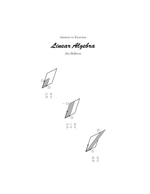
<strong>Answers</strong> to <strong>Exercises</strong><br />
<strong>Linear</strong> <strong>Algebra</strong><br />
Jim Hefferon<br />
( 1<br />
3)<br />
( 2<br />
1)<br />
∣ 1 2<br />
3 1∣<br />
x 1 ·<br />
( 1<br />
3<br />
)<br />
( 2<br />
1)<br />
∣ x · 1 2<br />
x · 3 1∣<br />
( 6<br />
8)<br />
( 2<br />
1)<br />
∣ 6 2<br />
8 1∣
Notation<br />
R real numbers<br />
N natural numbers: {0, 1, 2, . . .}<br />
C complex numbers<br />
{. . . ∣ . . .} set of . . . such that . . .<br />
〈. . .〉 sequence; like a set but order matters<br />
V, W, U vector spaces<br />
⃗v, ⃗w vectors<br />
⃗0, ⃗0 V zero vector, zero vector of V<br />
B, D bases<br />
E n = 〈⃗e 1 , . . . , ⃗e n 〉 standard basis for R n<br />
⃗β, ⃗ δ basis vectors<br />
Rep B (⃗v) matrix representing the vector<br />
P n set of n-th degree polynomials<br />
M n×m set of n×m matrices<br />
[S] span of the set S<br />
M ⊕ N direct sum of subspaces<br />
V ∼ = W isomorphic spaces<br />
h, g homomorphisms, linear maps<br />
H, G matrices<br />
t, s transformations; maps from a space to itself<br />
T, S square matrices<br />
Rep B,D (h) matrix representing the map h<br />
h i,j matrix entry from row i, column j<br />
|T | determinant of the matrix T<br />
R(h), N (h) rangespace and nullspace of the map h<br />
R ∞ (h), N ∞ (h) generalized rangespace and nullspace<br />
Lower case Greek alphabet<br />
name character name character name character<br />
alpha α iota ι rho ρ<br />
beta β kappa κ sigma σ<br />
gamma γ lambda λ tau τ<br />
delta δ mu µ upsilon υ<br />
epsilon ɛ nu ν phi φ<br />
zeta ζ xi ξ chi χ<br />
eta η omicron o psi ψ<br />
theta θ pi π omega ω<br />
Cover. This is Cramer’s Rule for the system x + 2y = 6, 3x + y = 8. The size of the first box is the determinant<br />
shown (the absolute value of the size is the area). The size of the second box is x times that, and equals the size<br />
of the final box. Hence, x is the final determinant divided by the first determinant.
These are answers to the exercises in <strong>Linear</strong> <strong>Algebra</strong> by J. Hefferon. Corrections or comments are<br />
very welcome, email to jimjoshua.smcvt.edu<br />
An answer labeled here as, for instance, One.II.3.4, matches the question numbered 4 from the first<br />
chapter, second section, and third subsection. The Topics are numbered separately.
Contents<br />
Chapter One: <strong>Linear</strong> Systems 3<br />
Subsection One.I.1: Gauss’ Method . . . . . . . . . . . . . . . . . . . . . . . . . . . . . . 5<br />
Subsection One.I.2: Describing the Solution Set . . . . . . . . . . . . . . . . . . . . . . . 10<br />
Subsection One.I.3: General = Particular + Homogeneous . . . . . . . . . . . . . . . . . 14<br />
Subsection One.II.1: Vectors in Space . . . . . . . . . . . . . . . . . . . . . . . . . . . . 17<br />
Subsection One.II.2: Length and Angle Measures . . . . . . . . . . . . . . . . . . . . . . 20<br />
Subsection One.III.1: Gauss-Jordan Reduction . . . . . . . . . . . . . . . . . . . . . . . 25<br />
Subsection One.III.2: Row Equivalence . . . . . . . . . . . . . . . . . . . . . . . . . . . . 27<br />
Topic: Computer <strong>Algebra</strong> Systems . . . . . . . . . . . . . . . . . . . . . . . . . . . . . . 31<br />
Topic: Input-Output Analysis . . . . . . . . . . . . . . . . . . . . . . . . . . . . . . . . . 33<br />
Topic: Accuracy of Computations . . . . . . . . . . . . . . . . . . . . . . . . . . . . . . . 33<br />
Topic: Analyzing Networks . . . . . . . . . . . . . . . . . . . . . . . . . . . . . . . . . . 33<br />
Chapter Two: Vector Spaces 36<br />
Subsection Two.I.1: Definition and Examples . . . . . . . . . . . . . . . . . . . . . . . . 37<br />
Subsection Two.I.2: Subspaces and Spanning Sets . . . . . . . . . . . . . . . . . . . . . 40<br />
Subsection Two.II.1: Definition and Examples . . . . . . . . . . . . . . . . . . . . . . . . 46<br />
Subsection Two.III.1: Basis . . . . . . . . . . . . . . . . . . . . . . . . . . . . . . . . . . 53<br />
Subsection Two.III.2: Dimension . . . . . . . . . . . . . . . . . . . . . . . . . . . . . . . 58<br />
Subsection Two.III.3: Vector Spaces and <strong>Linear</strong> Systems . . . . . . . . . . . . . . . . . . 61<br />
Subsection Two.III.4: Combining Subspaces . . . . . . . . . . . . . . . . . . . . . . . . . 66<br />
Topic: Fields . . . . . . . . . . . . . . . . . . . . . . . . . . . . . . . . . . . . . . . . . . 69<br />
Topic: Crystals . . . . . . . . . . . . . . . . . . . . . . . . . . . . . . . . . . . . . . . . . 70<br />
Topic: Voting Paradoxes . . . . . . . . . . . . . . . . . . . . . . . . . . . . . . . . . . . . 71<br />
Topic: Dimensional Analysis . . . . . . . . . . . . . . . . . . . . . . . . . . . . . . . . . . 72<br />
Chapter Three: Maps Between Spaces 74<br />
Subsection Three.I.1: Definition and Examples . . . . . . . . . . . . . . . . . . . . . . . 75<br />
Subsection Three.I.2: Dimension Characterizes Isomorphism . . . . . . . . . . . . . . . . 83<br />
Subsection Three.II.1: Definition . . . . . . . . . . . . . . . . . . . . . . . . . . . . . . . 85<br />
Subsection Three.II.2: Rangespace and Nullspace . . . . . . . . . . . . . . . . . . . . . . 90<br />
Subsection Three.III.1: Representing <strong>Linear</strong> Maps with Matrices . . . . . . . . . . . . . 95<br />
Subsection Three.III.2: Any Matrix Represents a <strong>Linear</strong> Map . . . . . . . . . . . . . . . 103<br />
Subsection Three.IV.1: Sums and Scalar Products . . . . . . . . . . . . . . . . . . . . . 107<br />
Subsection Three.IV.2: Matrix Multiplication . . . . . . . . . . . . . . . . . . . . . . . . 108<br />
Subsection Three.IV.3: Mechanics of Matrix Multiplication . . . . . . . . . . . . . . . . 112<br />
Subsection Three.IV.4: Inverses . . . . . . . . . . . . . . . . . . . . . . . . . . . . . . . . 116<br />
Subsection Three.V.1: Changing Representations of Vectors . . . . . . . . . . . . . . . . 121<br />
Subsection Three.V.2: Changing Map Representations . . . . . . . . . . . . . . . . . . . 124<br />
Subsection Three.VI.1: Orthogonal Projection Into a Line . . . . . . . . . . . . . . . . . 128<br />
Subsection Three.VI.2: Gram-Schmidt Orthogonalization . . . . . . . . . . . . . . . . . 131<br />
Subsection Three.VI.3: Projection Into a Subspace . . . . . . . . . . . . . . . . . . . . . 137<br />
Topic: Line of Best Fit . . . . . . . . . . . . . . . . . . . . . . . . . . . . . . . . . . . . . 143<br />
Topic: Geometry of <strong>Linear</strong> Maps . . . . . . . . . . . . . . . . . . . . . . . . . . . . . . . 147<br />
Topic: Markov Chains . . . . . . . . . . . . . . . . . . . . . . . . . . . . . . . . . . . . . 150<br />
Topic: Orthonormal Matrices . . . . . . . . . . . . . . . . . . . . . . . . . . . . . . . . . 157<br />
Chapter Four: Determinants 158<br />
Subsection Four.I.1: Exploration . . . . . . . . . . . . . . . . . . . . . . . . . . . . . . . 159<br />
Subsection Four.I.2: Properties of Determinants . . . . . . . . . . . . . . . . . . . . . . . 161<br />
Subsection Four.I.3: The Permutation Expansion . . . . . . . . . . . . . . . . . . . . . . 164<br />
Subsection Four.I.4: Determinants Exist . . . . . . . . . . . . . . . . . . . . . . . . . . . 166<br />
Subsection Four.II.1: Determinants as Size Functions . . . . . . . . . . . . . . . . . . . . 168<br />
Subsection Four.III.1: Laplace’s Expansion . . . . . . . . . . . . . . . . . . . . . . . . . 171
4 <strong>Linear</strong> <strong>Algebra</strong>, by Hefferon<br />
Topic: Cramer’s Rule . . . . . . . . . . . . . . . . . . . . . . . . . . . . . . . . . . . . . . 174<br />
Topic: Speed of Calculating Determinants . . . . . . . . . . . . . . . . . . . . . . . . . . 175<br />
Topic: Projective Geometry . . . . . . . . . . . . . . . . . . . . . . . . . . . . . . . . . . 176<br />
Chapter Five: Similarity 178<br />
Subsection Five.II.1: Definition and Examples . . . . . . . . . . . . . . . . . . . . . . . . 179<br />
Subsection Five.II.2: Diagonalizability . . . . . . . . . . . . . . . . . . . . . . . . . . . . 182<br />
Subsection Five.II.3: Eigenvalues and Eigenvectors . . . . . . . . . . . . . . . . . . . . . 186<br />
Subsection Five.III.1: Self-Composition . . . . . . . . . . . . . . . . . . . . . . . . . . . 190<br />
Subsection Five.III.2: Strings . . . . . . . . . . . . . . . . . . . . . . . . . . . . . . . . . 192<br />
Subsection Five.IV.1: Polynomials of Maps and Matrices . . . . . . . . . . . . . . . . . . 196<br />
Subsection Five.IV.2: Jordan Canonical Form . . . . . . . . . . . . . . . . . . . . . . . . 203<br />
Topic: Method of Powers . . . . . . . . . . . . . . . . . . . . . . . . . . . . . . . . . . . 210<br />
Topic: Stable Populations . . . . . . . . . . . . . . . . . . . . . . . . . . . . . . . . . . . 210<br />
Topic: <strong>Linear</strong> Recurrences . . . . . . . . . . . . . . . . . . . . . . . . . . . . . . . . . . . 210
Chapter One: <strong>Linear</strong> Systems<br />
Subsection One.I.1: Gauss’ Method<br />
One.I.1.16 Gauss’ method can be performed in different ways, so these simply exhibit one possible<br />
way to get the answer.<br />
(a) Gauss’ method<br />
−(1/2)ρ 1+ρ 2 2x + 3y = 7<br />
−→<br />
− (5/2)y = −15/2<br />
gives that the solution is y = 3 and x = 2.<br />
(b) Gauss’ method here<br />
−3ρ 1 +ρ 2<br />
−→<br />
gives x = −1, y = 4, and z = −1.<br />
One.I.1.17<br />
(a) Gaussian reduction<br />
1 3<br />
y = 4<br />
ρ +ρ<br />
x − z = 0<br />
y + 3z = 1<br />
x − z = 0<br />
−ρ 2 +ρ 3<br />
−→ y + 3z = 1<br />
−3z = 3<br />
−(1/2)ρ 1 +ρ 2<br />
−→<br />
2x + 2y = 5<br />
−5y = −5/2<br />
shows that y = 1/2 and x = 2 is the unique solution.<br />
(b) Gauss’ method<br />
gives y = 3/2 and x = 1/2 as the only solution.<br />
(c) Row reduction<br />
ρ 1+ρ 2<br />
−→<br />
−x + y = 1<br />
2y = 3<br />
−ρ 1 +ρ 2<br />
−→<br />
x − 3y + z = 1<br />
4y + z = 13<br />
shows, because the variable z is not a leading variable in any row, that there are many solutions.<br />
(d) Row reduction<br />
shows that there is no solution.<br />
(e) Gauss’ method<br />
−3ρ 1+ρ 2<br />
−→<br />
−x − y = 1<br />
0 = −1<br />
ρ 1 ↔ρ 4 2x − 2y + z = 0 −2ρ 1 +ρ 2 −4y + 3z = −20<br />
−→ −→<br />
x + z = 5 −ρ 1 +ρ 3 −y + 2z = −5<br />
x + y − z = 10 x + y − z = 10<br />
4y + z = 20<br />
4y + z = 20<br />
gives the unique solution (x, y, z) = (5, 5, 0).<br />
(f) Here Gauss’ method gives<br />
−2ρ 1+ρ 4 − (5/2)z − (5/2)w = −15/2<br />
2x + z + w = 5<br />
y − w = −1<br />
y − w = −1<br />
−(3/2)ρ 1 +ρ 3<br />
−→<br />
which shows that there are many solutions.<br />
−ρ 2 +ρ 4<br />
ρ 2 +ρ 4 (5/4)z = 0<br />
x + y − z = 10<br />
−4y + 3z = −20<br />
4z = 0<br />
−(1/4)ρ 2 +ρ 3<br />
−→<br />
−→<br />
y − w = −1<br />
− (5/2)z − (5/2)w = −15/2<br />
2x + z + w = 5<br />
0 = 0<br />
One.I.1.18 (a) From x = 1 − 3y we get that 2(1 − 3y) = −3, giving y = 1.<br />
(b) From x = 1 − 3y we get that 2(1 − 3y) + 2y = 0, leading to the conclusion that y = 1/2.<br />
Users of this method must check any potential solutions by substituting back into all the equations.
6 <strong>Linear</strong> <strong>Algebra</strong>, by Hefferon<br />
One.I.1.19 Do the reduction<br />
−3ρ 1+ρ 2 x − y = 1<br />
−→<br />
0 = −3 + k<br />
to conclude this system has no solutions if k ≠ 3 and if k = 3 then it has infinitely many solutions. It<br />
never has a unique solution.<br />
One.I.1.20 Let x = sin α, y = cos β, and z = tan γ:<br />
2x − y + 3z = 3<br />
2x − y + 3z = 3<br />
−2ρ 1+ρ 2<br />
4x + 2y − 2z = 10 −→ 4y − 8z = 4<br />
−3ρ<br />
6x − 3y + z = 9 1+ρ 3<br />
−8z = 0<br />
gives z = 0, y = 1, and x = 2. Note that no α satisfies that requirement.<br />
One.I.1.21<br />
(a) Gauss’ method<br />
x − 3y = b 1 x − 3y = b 1<br />
−3ρ 1 +ρ 2 10y = −3b −→<br />
1 + b 2 −ρ 2 +ρ 3 10y = −3b −→<br />
1 + b 2<br />
−ρ 1 3 10y = −b 1 + b 3 −ρ 2 +ρ 4 0 = 2b 1 − b 2 + b 3<br />
−2ρ 1+ρ 4<br />
10y = −2b 1 + b 4 0 = b 1 − b 2 + b 4<br />
shows that this system is consistent if and only if both b 3 = −2b 1 + b 2 and b 4 = −b 1 + b 2 .<br />
(b) Reduction<br />
x 1 + 2x 2 + 3x 3 = b 1 x 1 + 2x 2 + 3x 3 = b 1<br />
−2ρ 1 +ρ 2<br />
2ρ 2 +ρ 3<br />
−→ x 2 − 3x 3 = −2b 1 + b 2 −→ x 2 − 3x 3 = −2b 1 + b 2<br />
−ρ 1 +ρ 3<br />
−2x 2 + 5x 3 = −b 1 + b 3 −x 3 = −5b 1 + +2b 2 + b 3<br />
shows that each of b 1 , b 2 , and b 3 can be any real number — this system always has a unique solution.<br />
One.I.1.22 This system with more unknowns than equations<br />
x + y + z = 0<br />
x + y + z = 1<br />
has no solution.<br />
One.I.1.23 Yes. For example, the fact that the same reaction can be performed in two different flasks<br />
shows that twice any solution is another, different, solution (if a physical reaction occurs then there<br />
must be at least one nonzero solution).<br />
One.I.1.24<br />
Gauss’ method<br />
Because f(1) = 2, f(−1) = 6, and f(2) = 3 we get a linear system.<br />
a + b + c = 2<br />
−ρ 1+ρ 2<br />
−→ −2b = 4<br />
−4ρ 1 +ρ 2<br />
−2b − 3c = −5<br />
shows that the solution is f(x) = 1x 2 − 2x + 3.<br />
1a + 1b + c = 2<br />
1a − 1b + c = 6<br />
4a + 2b + c = 3<br />
a + b + c = 2<br />
−ρ 2+ρ 3<br />
−→ −2b = 4<br />
−3c = −9<br />
One.I.1.25 (a) Yes, by inspection the given equation results from −ρ 1 + ρ 2 .<br />
(b) No. The given equation is satisfied by the pair (1, 1). However, that pair does not satisfy the<br />
first equation in the system.<br />
(c) Yes. To see if the given row is c 1 ρ 1 + c 2 ρ 2 , solve the system of equations relating the coefficients<br />
of x, y, z, and the constants:<br />
2c 1 + 6c 2 = 6<br />
c 1 − 3c 2 = −9<br />
−c 1 + c 2 = 5<br />
4c 1 + 5c 2 = −2<br />
and get c 1 = −3 and c 2 = 2, so the given row is −3ρ 1 + 2ρ 2 .<br />
One.I.1.26 If a ≠ 0 then the solution set of the first equation is {(x, y) ∣ ∣ x = (c − by)/a}. Taking y = 0<br />
gives the solution (c/a, 0), and since the second equation is supposed to have the same solution set,<br />
substituting into it gives that a(c/a) + d · 0 = e, so c = e. Then taking y = 1 in x = (c − by)/a gives<br />
that a((c − b)/a) + d · 1 = e, which gives that b = d. Hence they are the same equation.<br />
When a = 0 the equations can be different and still have the same solution set: e.g., 0x + 3y = 6<br />
and 0x + 6y = 12.
<strong>Answers</strong> to <strong>Exercises</strong> 7<br />
One.I.1.27 We take three cases, first that a =≠ 0, second that a = 0 and c ≠ 0, and third that both<br />
a = 0 and c = 0.<br />
For the first, we assume that a ≠ 0. Then the reduction<br />
−(c/a)ρ 1+ρ 2<br />
ax + by = j<br />
−→<br />
(− cb<br />
a + d)y = − cj a + k<br />
shows that this system has a unique solution if and only if −(cb/a) + d ≠ 0; remember that a ≠ 0<br />
so that back substitution yields a unique x (observe, by the way, that j and k play no role in the<br />
conclusion that there is a unique solution, although if there is a unique solution then they contribute<br />
to its value). But −(cb/a)+d = (ad−bc)/a and a fraction is not equal to 0 if and only if its numerator<br />
is not equal to 0. This, in this first case, there is a unique solution if and only if ad − bc ≠ 0.<br />
In the second case, if a = 0 but c ≠ 0, then we swap<br />
cx + dy = k<br />
by = j<br />
to conclude that the system has a unique solution if and only if b ≠ 0 (we use the case assumption that<br />
c ≠ 0 to get a unique x in back substitution). But — where a = 0 and c ≠ 0 — the condition “b ≠ 0”<br />
is equivalent to the condition “ad − bc ≠ 0”. That finishes the second case.<br />
Finally, for the third case, if both a and c are 0 then the system<br />
0x + by = j<br />
0x + dy = k<br />
might have no solutions (if the second equation is not a multiple of the first) or it might have infinitely<br />
many solutions (if the second equation is a multiple of the first then for each y satisfying both equations,<br />
any pair (x, y) will do), but it never has a unique solution. Note that a = 0 and c = 0 gives that<br />
ad − bc = 0.<br />
One.I.1.28 Recall that if a pair of lines share two distinct points then they are the same line. That’s<br />
because two points determine a line, so these two points determine each of the two lines, and so they<br />
are the same line.<br />
Thus the lines can share one point (giving a unique solution), share no points (giving no solutions),<br />
or share at least two points (which makes them the same line).<br />
One.I.1.29 For the reduction operation of multiplying ρ i by a nonzero real number k, we have that<br />
(s 1 , . . . , s n ) satisfies this system<br />
a 1,1 x 1 + a 1,2 x 2 + · · · + a 1,n x n = d 1<br />
if and only if<br />
ka i,1 x 1 + ka i,2 x 2 + · · · + ka i,n x n = kd i<br />
.<br />
a m,1 x 1 + a m,2 x 2 + · · · + a m,n x n = d m<br />
.<br />
a 1,1 s 1 + a 1,2 s 2 + · · · + a 1,n s n = d 1<br />
.<br />
and ka i,1 s 1 + ka i,2 s 2 + · · · + ka i,n s n = kd i<br />
.<br />
and a m,1 s 1 + a m,2 s 2 + · · · + a m,n s n = d m<br />
by the definition of ‘satisfies’. But, because k ≠ 0, that’s true if and only if<br />
a 1,1 s 1 + a 1,2 s 2 + · · · + a 1,n s n = d 1<br />
.<br />
.<br />
and a i,1 s 1 + a i,2 s 2 + · · · + a i,n s n = d i<br />
.<br />
.<br />
and a m,1 s 1 + a m,2 s 2 + · · · + a m,n s n = d m
8 <strong>Linear</strong> <strong>Algebra</strong>, by Hefferon<br />
(this is straightforward cancelling on both sides of the i-th equation), which says that (s 1 , . . . , s n )<br />
solves<br />
a 1,1 x 1 + a 1,2 x 2 + · · · + a 1,n x n = d 1<br />
.<br />
.<br />
a i,1 x 1 + a i,2 x 2 + · · · + a i,n x n = d i<br />
a m,1 x 1 + a m,2 x 2 + · · · + a m,n x n = d m<br />
as required.<br />
For the pivot operation kρ i + ρ j , we have that (s 1 , . . . , s n ) satisfies<br />
a 1,1 x 1 + · · · + a 1,n x n = d 1<br />
.<br />
a i,1 x 1 + · · · + a i,n x n = d i<br />
.<br />
.<br />
(ka i,1 + a j,1 )x 1 + · · · + (ka i,n + a j,n )x n = kd i + d j<br />
if and only if<br />
a m,1 x 1 + · · · +<br />
a m,n x n = d m<br />
a 1,1 s 1 + · · · + a 1,n s n = d 1<br />
.<br />
and a i,1 s 1 + · · · + a i,n s n = d i<br />
.<br />
and (ka i,1 + a j,1 )s 1 + · · · + (ka i,n + a j,n )s n = kd i + d j<br />
and a m,1 s 1 + a m,2 s 2 + · · · + a m,n s n = d m<br />
again by the definition of ‘satisfies’. Subtract k times the i-th equation from the j-th equation (remark:<br />
here is where i ≠ j is needed; if i = j then the two d i ’s above are not equal) to get that the<br />
previous compound statement holds if and only if<br />
a 1,1 s 1 + · · · + a 1,n s n = d 1<br />
.<br />
.<br />
and a i,1 s 1 + · · · + a i,n s n = d i<br />
.<br />
.<br />
and (ka i,1 + a j,1 )s 1 + · · · + (ka i,n + a j,n )s n<br />
− (ka i,1 s 1 + · · · + ka i,n s n ) = kd i + d j − kd i<br />
.<br />
.<br />
and a m,1 s 1 + · · · + a m,n s n = d m<br />
which, after cancellation, says that (s 1 , . . . , s n ) solves<br />
a 1,1 x 1 + · · · + a 1,n x n = d 1<br />
.<br />
a i,1 x 1 + · · · + a i,n x n = d i<br />
.<br />
.<br />
a j,1 x 1 + · · · + a j,n x n = d j<br />
.<br />
.<br />
a m,1 x 1 + · · · + a m,n x n = d m<br />
as required.<br />
One.I.1.30<br />
Yes, this one-equation system:<br />
is satisfied by every (x, y) ∈ R 2 .<br />
0x + 0y = 0<br />
.<br />
.<br />
.
<strong>Answers</strong> to <strong>Exercises</strong> 9<br />
One.I.1.31<br />
Yes. This sequence of operations swaps rows i and j<br />
ρ i +ρ j<br />
−→<br />
−ρ j +ρ i<br />
−→<br />
ρ i +ρ j<br />
−→<br />
−1ρ i<br />
−→<br />
so the row-swap operation is redundant in the presence of the other two.<br />
One.I.1.32<br />
Swapping rows is reversed by swapping back.<br />
a 1,1 x 1 + · · · + a 1,n x n = d 1<br />
.<br />
a m,1 x 1 + · · · + a m,n x n = d m<br />
ρ i ↔ρ j ρ j ↔ρ i<br />
−→ −→<br />
a 1,1 x 1 + · · · + a 1,n x n = d 1<br />
.<br />
a m,1 x 1 + · · · + a m,n x n = d m<br />
Multiplying both sides of a row by k ≠ 0 is reversed by dividing by k.<br />
a 1,1 x 1 + · · · + a 1,n x n = d 1<br />
.<br />
.<br />
a m,1 x 1 + · · · + a m,n x n = d m<br />
a 1,1 x 1 + · · · + a 1,n x n = d 1<br />
−→<br />
.<br />
.<br />
a m,1 x 1 + · · · + a m,n x n = d m<br />
kρ i<br />
−→<br />
(1/k)ρ i<br />
Adding k times a row to another is reversed by adding −k times that row.<br />
a 1,1 x 1 + · · · + a 1,n x n = d 1<br />
.<br />
a m,1 x 1 + · · · + a m,n x n = d m<br />
kρ i+ρ j<br />
−→<br />
−kρ i+ρ j<br />
a 1,1 x 1 + · · · + a 1,n x n = d 1<br />
−→ .<br />
a m,1 x 1 + · · · + a m,n x n = d m<br />
Remark: observe for the third case that if we were to allow i = j then the result wouldn’t hold.<br />
3x + 2y = 7 2ρ 1+ρ 1<br />
−2ρ 1 +ρ 1<br />
−→ 9x + 6y = 21 −→<br />
−9x − 6y = −21<br />
One.I.1.33 Let p, n, and d be the number of pennies, nickels, and dimes. For variables that are real<br />
numbers, this system<br />
p + n + d = 13<br />
p + 5n + 10d = 83<br />
−ρ 1+ρ 2<br />
−→<br />
p + n + d = 13<br />
4n + 9d = 70<br />
has infinitely many solutions. However, it has a limited number of solutions in which p, n, and d are<br />
non-negative integers. Running through d = 0, . . . , d = 8 shows that (p, n, d) = (3, 4, 6) is the only<br />
sensible solution.<br />
One.I.1.34<br />
Solving the system<br />
(1/3)(a + b + c) + d = 29<br />
(1/3)(b + c + d) + a = 23<br />
(1/3)(c + d + a) + b = 21<br />
(1/3)(d + a + b) + c = 17<br />
we obtain a = 12, b = 9, c = 3, d = 21. Thus the second item, 21, is the correct answer.<br />
One.I.1.35 This is how the answer was given in the cited source. A comparison of the units and<br />
hundreds columns of this addition shows that there must be a carry from the tens column. The tens<br />
column then tells us that A < H, so there can be no carry from the units or hundreds columns. The<br />
five columns then give the following five equations.<br />
A + E = W<br />
2H = A + 10<br />
H = W + 1<br />
H + T = E + 10<br />
A + 1 = T<br />
The five linear equations in five unknowns, if solved simultaneously, produce the unique solution: A =<br />
4, T = 5, H = 7, W = 6 and E = 2, so that the original example in addition was 47474+5272 = 52746.<br />
One.I.1.36 This is how the answer was given in the cited source. Eight commissioners voted for B.<br />
To see this, we will use the given information to study how many voters chose each order of A, B, C.<br />
The six orders of preference are ABC, ACB, BAC, BCA, CAB, CBA; assume they receive a, b,<br />
c, d, e, f votes respectively. We know that<br />
a + b + e = 11<br />
d + e + f = 12<br />
a + c + d = 14
10 <strong>Linear</strong> <strong>Algebra</strong>, by Hefferon<br />
from the number preferring A over B, the number preferring C over A, and the number preferring B<br />
over C. Because 20 votes were cast, we also know that<br />
c + d + f = 9<br />
a + b + c = 8<br />
b + e + f = 6<br />
from the preferences for B over A, for A over C, and for C over B.<br />
The solution is a = 6, b = 1, c = 1, d = 7, e = 4, and f = 1. The number of commissioners voting<br />
for B as their first choice is therefore c + d = 1 + 7 = 8.<br />
Comments. The answer to this question would have been the same had we known only that at least<br />
14 commissioners preferred B over C.<br />
The seemingly paradoxical nature of the commissioners’s preferences (A is preferred to B, and B is<br />
preferred to C, and C is preferred to A), an example of “non-transitive dominance”, is not uncommon<br />
when individual choices are pooled.<br />
One.I.1.37 This is how the answer was given in the cited source. We have not used “dependent” yet;<br />
it means here that Gauss’ method shows that there is not a unique solution. If n ≥ 3 the system is<br />
dependent and the solution is not unique. Hence n < 3. But the term “system” implies n > 1. Hence<br />
n = 2. If the equations are<br />
ax + (a + d)y = a + 2d<br />
(a + 3d)x + (a + 4d)y = a + 5d<br />
then x = −1, y = 2.<br />
Subsection One.I.2: Describing the Solution Set<br />
One.I.2.15 (a) 2 (b) 3 (c) −1 (d) Not defined.<br />
One.I.2.16 (a) 2×3 (b) 3×2 (c) 2×2<br />
⎛<br />
One.I.2.17 (a) ⎝ 5 ⎞<br />
⎛<br />
( )<br />
1⎠<br />
20<br />
(b) (c) ⎝ −2<br />
⎞<br />
4 ⎠<br />
−5<br />
⎛ ⎞<br />
5<br />
0<br />
(f)<br />
⎝ 12 8<br />
4<br />
⎠<br />
(d)<br />
( )<br />
41<br />
52<br />
(e) Not defined.<br />
One.I.2.18 (a) This reduction (3 )<br />
6 18<br />
1 2 6<br />
( )<br />
(−1/3)ρ 1 +ρ 2 3 6 18<br />
−→<br />
0 0 0<br />
leaves x leading and y free. Making y the parameter, we have x = 6 − 2y so the solution set is<br />
( ( )<br />
6 −2<br />
{ + y<br />
0)<br />
∣ y ∈ R}.<br />
1<br />
(b) This reduction<br />
(<br />
1 1<br />
)<br />
1<br />
1 −1 −1<br />
( )<br />
−ρ 1 +ρ 2 1 1 1<br />
−→<br />
0 −2 −2<br />
gives the unique solution y = 1, x = 0. The solution set is<br />
(<br />
0<br />
{ }.<br />
1)<br />
(c) This use of Gauss’ method<br />
⎛<br />
⎝ 1 0 1 4<br />
⎞ ⎛<br />
1 −1 2 5 ⎠ −ρ 1+ρ 2<br />
−→ ⎝ 1 0 1 4<br />
⎞<br />
0 −1 1 1 −→<br />
−4ρ<br />
4 −1 5 17<br />
1+ρ 3<br />
0 −1 1 1<br />
leaves x 1 and x 2 leading with x 3 free. The solution set is<br />
⎛<br />
{ ⎝ 4<br />
⎞ ⎛<br />
−1⎠ + ⎝ −1<br />
⎞<br />
∣<br />
1 ⎠ x 3 x 3 ∈ R}.<br />
0 1<br />
⎠ −ρ 2+ρ 3<br />
⎛<br />
⎝ 1 0 1 4<br />
⎞<br />
0 −1 1 1⎠<br />
0 0 0 0
<strong>Answers</strong> to <strong>Exercises</strong> 11<br />
(d) This reduction<br />
⎛<br />
⎝ 2 1 −1 2<br />
⎞<br />
2 0 1 3⎠<br />
1 −1 0 0<br />
−ρ1+ρ2<br />
−→<br />
−(1/2)ρ 1 +ρ 3<br />
shows that the solution set is a singleton set.<br />
(e) This reduction is easy<br />
⎛<br />
⎝ 1 2 −1 0 3<br />
⎞<br />
2 1 0 1 4<br />
1 −1 1 1 1<br />
⎠ −2ρ1+ρ2<br />
−→<br />
−ρ 1+ρ 3<br />
⎛<br />
⎝ 2 1 −1 2<br />
⎞<br />
0 −1 2 1<br />
0 −3/2 1/2 −1<br />
⎛<br />
⎞<br />
{ ⎝ 1 1⎠}<br />
1<br />
⎛<br />
⎝ 1 2 −1 0 3<br />
⎞<br />
0 −3 2 1 −2<br />
0 −3 2 1 −2<br />
⎠ (−3/2)ρ2+ρ3<br />
−→<br />
⎠ −ρ2+ρ3<br />
−→<br />
⎛<br />
⎝ 2 0 1 −1 −1 2 2<br />
1<br />
⎞<br />
⎠<br />
0 0 −5/2 −5/2<br />
⎛<br />
⎝ 1 2 −1 0 3<br />
⎞<br />
0 −3 2 1 −2⎠<br />
0 0 0 0 0<br />
and ends with x and y leading, while z and w are free. Solving for y gives y = (2 + 2z + w)/3 and<br />
substitution shows that x + 2(2 + 2z + w)/3 − z = 3 so x = (5/3) − (1/3)z − (2/3)w, making the<br />
solution set<br />
⎛ ⎞ ⎞<br />
⎞<br />
(f) The reduction<br />
⎛<br />
⎝ 1 0 1 1 4<br />
⎞<br />
2 1 0 −1 2<br />
3 1 1 0 7<br />
⎛<br />
⎛<br />
5/3 −1/3 −2/3<br />
{ ⎜2/3<br />
⎟<br />
⎝ 0 ⎠ + ⎜ 2/3<br />
⎟<br />
⎝ 1 ⎠ z + ⎜ 1/3<br />
⎝ 0<br />
0 0<br />
1<br />
⎠ −2ρ1+ρ2<br />
−→<br />
−3ρ 1 +ρ 3<br />
⎛<br />
⎝ 1 0 1 1 4<br />
⎞<br />
0 1 −2 −3 −6<br />
0 1 −2 −3 −5<br />
shows that there is no solution — the solution set is empty.<br />
One.I.2.19<br />
(a) This reduction<br />
( )<br />
2 1 −1 1<br />
4 −1 0 3<br />
⎟<br />
⎠ w ∣ ∣ z, w ∈ R}.<br />
⎠ −ρ2+ρ3<br />
−→<br />
( )<br />
−2ρ 1 +ρ 2 2 1 −1 1<br />
−→<br />
0 −3 2 1<br />
⎛<br />
⎝ 1 0 1 1 4<br />
⎞<br />
0 1 −2 −3 −6⎠<br />
0 0 0 0 1<br />
ends with x and y leading while z is free. Solving for y gives y = (1−2z)/(−3), and then substitution<br />
2x + (1 − 2z)/(−3) − z = 1 shows that x = ((4/3) + (1/3)z)/2. Hence the solution set is<br />
⎛<br />
{ ⎝ 2/3<br />
⎞ ⎛<br />
−1/3⎠ + ⎝ 1/6<br />
⎞<br />
2/3⎠ z ∣ z ∈ R}.<br />
0 1<br />
(b) This application of Gauss’ method<br />
⎛<br />
⎝ 1 0 −1 0 1 ⎞ ⎛<br />
0 1 2 −1 3⎠ −ρ 1+ρ 3<br />
−→ ⎝ 1 0 −1 0 1 ⎞<br />
0 1 2 −1 3<br />
1 2 3 −1 7<br />
0 2 4 −1 6<br />
leaves x, y, and w leading. The solution set is<br />
⎛ ⎞ ⎛ ⎞<br />
1 1<br />
{ ⎜3<br />
⎟<br />
⎝0⎠ + ⎜−2<br />
⎟<br />
⎝ 1 ⎠ z ∣ z ∈ R}.<br />
0 0<br />
(c) This row reduction<br />
⎛<br />
⎞<br />
1 −1 1 0 0<br />
⎜0 1 0 1 0<br />
⎟<br />
⎝3 −2 3 1 0⎠<br />
0 −1 0 −1 0<br />
−3ρ 1+ρ 3<br />
−→<br />
⎛<br />
⎞<br />
1 −1 1 0 0<br />
⎜0 1 0 1 0<br />
⎟<br />
⎝0 1 0 1 0⎠<br />
0 −1 0 −1 0<br />
⎠ −2ρ 2+ρ 3<br />
−→<br />
−ρ 2+ρ 3<br />
−→<br />
ρ 2+ρ 4<br />
ends with z and w free. The solution set is<br />
⎛ ⎞ ⎛ ⎞ ⎛ ⎞<br />
0 −1 −1<br />
{ ⎜0<br />
⎟<br />
⎝0⎠ + ⎜ 0<br />
⎟<br />
⎝ 1 ⎠ z + ⎜−1<br />
⎟<br />
⎝ 0 ⎠ w ∣ z, w ∈ R}.<br />
0 0 1<br />
⎛<br />
⎝ 1 0 −1 0 1 ⎞<br />
0 1 2 −1 3⎠<br />
0 0 0 1 0<br />
⎛<br />
⎞<br />
1 −1 1 0 0<br />
⎜0 1 0 1 0<br />
⎟<br />
⎝0 0 0 0 0⎠<br />
0 0 0 0 0
12 <strong>Linear</strong> <strong>Algebra</strong>, by Hefferon<br />
(d) Gauss’ method done in this way<br />
( )<br />
1 2 3 1 −1 1<br />
3 −1 1 1 1 3<br />
( )<br />
−3ρ 1 +ρ 2 1 2 3 1 −1 1<br />
−→<br />
0 −7 −8 −2 4 0<br />
ends with c, d, and e free. Solving for b shows that b = (8c + 2d − 4e)/(−7) and then substitution<br />
a + 2(8c + 2d − 4e)/(−7) + 3c + 1d − 1e = 1 shows that a = 1 − (5/7)c − (3/7)d − (1/7)e and so the<br />
solution set is ⎛ ⎞ ⎛ ⎞ ⎛ ⎞ ⎛ ⎞<br />
1 −5/7 −3/7 −1/7<br />
0<br />
{<br />
⎜0<br />
⎟<br />
⎝0⎠ + −8/7<br />
⎜ 1<br />
⎟<br />
⎝ 0 ⎠ c + −2/7<br />
⎜ 0<br />
⎟<br />
⎝ 1 ⎠ d + 4/7<br />
⎜ 0<br />
⎟<br />
⎝ 0 ⎠ e ∣ c, d, e ∈ R}.<br />
0 0<br />
0<br />
1<br />
One.I.2.20 For each problem we get a system of linear equations by looking at the equations of<br />
components.<br />
(a) k = 5<br />
(b) The second components show that i = 2, the third components show that j = 1.<br />
(c) m = −4, n = 2<br />
One.I.2.21 For each problem we get a system of linear equations by looking at the equations of<br />
components.<br />
(a) Yes; take k = −1/2.<br />
(b) No; the system with equations 5 = 5 · j and 4 = −4 · j has no solution.<br />
(c) Yes; take r = 2.<br />
(d) No. The second components give k = 0. Then the third components give j = 1. But the first<br />
components don’t check.<br />
One.I.2.22<br />
This system has 1 equation. The leading variable is x 1 , the other variables are free.<br />
⎛ ⎞ ⎛ ⎞<br />
−1<br />
−1<br />
1<br />
{ ⎜ . ⎟<br />
⎝ . ⎠ x 0<br />
2 + · · · + ⎜ . ⎟<br />
⎝ . ⎠ x ∣<br />
n x 1 , . . . , x n ∈ R}<br />
0<br />
1<br />
One.I.2.23 (a) Gauss’ method here gives<br />
⎛<br />
⎝ 1 2 0 −1 a<br />
⎞<br />
2 0 1 0 b⎠<br />
−2ρ1+ρ2<br />
−→<br />
−ρ<br />
1 1 0 2 c<br />
1+ρ 3<br />
−(1/4)ρ 2+ρ 3<br />
−→<br />
⎛<br />
⎝ 1 2 0 −1 a<br />
⎞<br />
0 −4 1 2 −2a + b⎠<br />
0 −1 0 3 −a + c<br />
⎛<br />
⎝ 1 2 0 −1 a<br />
⎞<br />
0 −4 1 2 −2a + b ⎠ ,<br />
0 0 −1/4 5/2 −(1/2)a − (1/4)b + c<br />
leaving w free. Solve: z = 2a + b − 4c + 10w, and −4y = −2a + b − (2a + b − 4c + 10w) − 2w so<br />
y = a − c + 3w, and x = a − 2(a − c + 3w) + w = −a + 2c − 5w. Therefore the solution set is this.<br />
⎛ ⎞ ⎛ ⎞<br />
−a + 2c −5<br />
{ ⎜ a − c<br />
⎟<br />
⎝2a + b − 4c⎠ + ⎜ 3<br />
⎟<br />
⎝ 10 ⎠ w ∣ w ∈ R}<br />
0<br />
1<br />
(b) Plug in with a = 3, b = 1, and c = −2.<br />
⎛ ⎞ ⎛ ⎞<br />
−7 −5<br />
{ ⎜ 5<br />
⎟<br />
⎝ 15 ⎠ + ⎜ 3<br />
⎟<br />
⎝ 10 ⎠ w ∣ w ∈ R}<br />
0 1<br />
One.I.2.24<br />
a 12,3 .<br />
One.I.2.25<br />
Leaving the comma out, say by writing a 123 , is ambiguous because it could mean a 1,23 or<br />
(a)<br />
⎛<br />
⎞<br />
2 3 4 5<br />
⎜3 4 5 6<br />
⎟<br />
⎝4 5 6 7⎠<br />
5 6 7 8<br />
⎛<br />
⎞<br />
1 −1 1 −1<br />
(b) ⎜−1 1 −1 1<br />
⎟<br />
⎝ 1 −1 1 −1⎠<br />
−1 1 −1 1
<strong>Answers</strong> to <strong>Exercises</strong> 13<br />
⎛<br />
One.I.2.26 (a) ⎝ 1 4<br />
⎞<br />
( ) ( )<br />
2 5⎠<br />
2 1<br />
5 10<br />
(b)<br />
(c)<br />
(d) ( 1 1 0 )<br />
−3 1 10 5<br />
3 6<br />
One.I.2.27<br />
(a) Plugging in x = 1 and x = −1 gives<br />
a + b + c = 2<br />
a − b + c = 6<br />
−ρ 1 +ρ 2<br />
−→<br />
a + b + c = 2<br />
−2b = 4<br />
so the set of functions is {f(x) = (4 − c)x 2 − 2x + c ∣ ∣ c ∈ R}.<br />
(b) Putting in x = 1 gives<br />
a + b + c = 2<br />
so the set of functions is {f(x) = (2 − b − c)x 2 + bx + c ∣ ∣ b, c ∈ R}.<br />
One.I.2.28 On plugging in the five pairs (x, y) we get a system with the five equations and six unknowns<br />
a, . . . , f. Because there are more unknowns than equations, if no inconsistency exists among the<br />
equations then there are infinitely many solutions (at least one variable will end up free).<br />
But no inconsistency can exist because a = 0, . . . , f = 0 is a solution (we are only using this zero<br />
solution to show that the system is consistent — the prior paragraph shows that there are nonzero<br />
solutions).<br />
One.I.2.29 (a) Here is one — the fourth equation is redundant but still OK.<br />
x + y − z + w = 0<br />
y − z = 0<br />
2z + 2w = 0<br />
z + w = 0<br />
(b) Here is one.<br />
x + y − z + w = 0<br />
w = 0<br />
w = 0<br />
w = 0<br />
(c) This is one.<br />
x + y − z + w = 0<br />
x + y − z + w = 0<br />
x + y − z + w = 0<br />
x + y − z + w = 0<br />
One.I.2.30 This is how the answer was given in the cited source.<br />
(a) Formal solution of the system yields<br />
x = a3 − 1<br />
a 2 y = −a2 + a<br />
− 1 a 2 − 1 .<br />
If a + 1 ≠ 0 and a − 1 ≠ 0, then the system has the single solution<br />
x = a2 + a + 1<br />
y =<br />
−a<br />
a + 1<br />
a + 1 .<br />
If a = −1, or if a = +1, then the formulas are meaningless; in the first instance we arrive at the<br />
system { −x + y = 1<br />
x − y = 1<br />
which is a contradictory system. In the second instance we have<br />
{<br />
x + y = 1<br />
x + y = 1<br />
which has an infinite number of solutions (for example, for x arbitrary, y = 1 − x).<br />
(b) Solution of the system yields<br />
x = a4 − 1<br />
a 2 y = −a3 + a<br />
− 1 a 2 − 1 .<br />
Here, is a 2 − 1 ≠ 0, the system has the single solution x = a 2 + 1, y = −a. For a = −1 and a = 1,<br />
we obtain the systems<br />
{ { −x + y = −1 x + y = 1<br />
x − y = 1 x + y = 1<br />
both of which have an infinite number of solutions.
14 <strong>Linear</strong> <strong>Algebra</strong>, by Hefferon<br />
One.I.2.31 This is how the answer was given in the cited source. Let u, v, x, y, z be the volumes<br />
in cm 3 of Al, Cu, Pb, Ag, and Au, respectively, contained in the sphere, which we assume to be<br />
not hollow. Since the loss of weight in water (specific gravity 1.00) is 1000 grams, the volume of the<br />
sphere is 1000 cm 3 . Then the data, some of which is superfluous, though consistent, leads to only 2<br />
independent equations, one relating volumes and the other, weights.<br />
u + v + x + y + z = 1000<br />
2.7u + 8.9v + 11.3x + 10.5y + 19.3z = 7558<br />
Clearly the sphere must contain some aluminum to bring its mean specific gravity below the specific<br />
gravities of all the other metals. There is no unique result to this part of the problem, for the amounts<br />
of three metals may be chosen arbitrarily, provided that the choices will not result in negative amounts<br />
of any metal.<br />
If the ball contains only aluminum and gold, there are 294.5 cm 3 of gold and 705.5 cm 3 of aluminum.<br />
Another possibility is 124.7 cm 3 each of Cu, Au, Pb, and Ag and 501.2 cm 3 of Al.<br />
Subsection One.I.3: General = Particular + Homogeneous<br />
One.I.3.15 For the arithmetic to these, see the answers from the prior subsection.<br />
(a) The solution set is<br />
( ( )<br />
6 −2<br />
{ + y<br />
0)<br />
∣ y ∈ R}.<br />
1<br />
Here the particular solution and the<br />
(<br />
solution set<br />
(<br />
for<br />
)<br />
the associated homogeneous system are<br />
6 −2<br />
and { y<br />
0)<br />
∣ y ∈ R}.<br />
1<br />
(b) The solution set is<br />
(<br />
0<br />
{ }.<br />
1)<br />
The particular solution and the solution<br />
(<br />
set for the associated<br />
(<br />
homogeneous system are<br />
0 0<br />
and { }<br />
1)<br />
0)<br />
(c) The solution set is<br />
⎛<br />
{ ⎝ 4<br />
⎞ ⎛<br />
−1⎠ + ⎝ −1<br />
⎞<br />
∣<br />
1 ⎠ x 3 x3 ∈ R}.<br />
0 1<br />
A particular solution and the solution<br />
⎛<br />
set for the associated homogeneous system are<br />
⎝ 4 ⎞ ⎛<br />
−1⎠ and { ⎝ −1<br />
⎞<br />
∣<br />
1 ⎠ x 3 x 3 ∈ R}.<br />
0<br />
1<br />
(d) The solution set is a singleton<br />
⎛ ⎞<br />
{ ⎝ 1 1⎠}.<br />
1<br />
A particular solution and the solution<br />
⎛ ⎞<br />
set for the<br />
⎛<br />
associated<br />
⎞<br />
homogeneous system are<br />
⎝ 1 1⎠ and { ⎝ 0 0⎠ t ∣ t ∈ R}.<br />
1<br />
0<br />
(e) The solution set is<br />
⎛ ⎞ ⎛ ⎞ ⎛ ⎞<br />
5/3 −1/3 −2/3<br />
{ ⎜2/3<br />
⎟<br />
⎝ 0 ⎠ + ⎜ 2/3<br />
⎟<br />
⎝ 1 ⎠ z + ⎜ 1/3<br />
⎟<br />
⎝ 0 ⎠ w ∣ z, w ∈ R}.<br />
0 0<br />
1<br />
A particular solution and<br />
⎛<br />
the<br />
⎞<br />
solution set<br />
⎛<br />
for the<br />
⎞<br />
associated<br />
⎛ ⎞<br />
homogeneous system are<br />
5/2<br />
−1/3 −2/3<br />
⎜2/3<br />
⎟<br />
⎝ 0 ⎠ and { ⎜ 2/3<br />
⎟<br />
⎝ 1 ⎠ z + ⎜ 1/3<br />
⎟<br />
⎝ 0 ⎠ w ∣ z, w ∈ R}.<br />
0<br />
0<br />
1
<strong>Answers</strong> to <strong>Exercises</strong> 15<br />
(f) This system’s solution set is empty. Thus, there is no particular solution. The solution set of the<br />
associated homogeneous system is<br />
⎛ ⎞ ⎛ ⎞<br />
−1 −1<br />
{ ⎜ 2<br />
⎟<br />
⎝ 1 ⎠ z + ⎜ 3<br />
⎟<br />
⎝ 0 ⎠ w ∣ z, w ∈ R}.<br />
0 1<br />
One.I.3.16 The answers from the prior subsection show the row operations.<br />
(a) The solution set is<br />
⎛<br />
{ ⎝ 2/3<br />
⎞ ⎛<br />
−1/3⎠ + ⎝ 1/6<br />
⎞<br />
2/3⎠ z ∣ z ∈ R}.<br />
0 1<br />
A particular solution and the solution set for the associated homogeneous system are<br />
⎛<br />
⎝ 2/3<br />
⎞ ⎛ ⎞<br />
1/6<br />
−1/3⎠ and { ⎝2/3⎠ z ∣ z ∈ R}.<br />
0<br />
1<br />
(b) The solution set is<br />
⎛ ⎞ ⎛ ⎞<br />
1 1<br />
{ ⎜3<br />
⎟<br />
⎝0⎠ + ⎜−2<br />
⎟<br />
⎝ 1 ⎠ z ∣ z ∈ R}.<br />
0 0<br />
A particular solution and the solution set for the associated homogeneous system are<br />
⎛ ⎞ ⎛ ⎞<br />
1<br />
1<br />
⎜3<br />
⎟<br />
⎝0⎠ and { ⎜−2<br />
⎟<br />
⎝ 1 ⎠ z ∣ z ∈ R}.<br />
0<br />
0<br />
(c) The solution set is ⎛ ⎞ ⎛ ⎞ ⎛ ⎞<br />
0 −1 −1<br />
{ ⎜0<br />
⎟<br />
⎝0⎠ + ⎜ 0<br />
⎟<br />
⎝ 1 ⎠ z + ⎜−1<br />
⎟<br />
⎝ 0 ⎠ w ∣ z, w ∈ R}.<br />
0 0 1<br />
A particular solution and the solution set for the associated homogeneous system are<br />
⎛ ⎞ ⎛ ⎞ ⎛ ⎞<br />
0<br />
−1 −1<br />
⎜0<br />
⎟<br />
⎝0⎠ and { ⎜ 0<br />
⎟<br />
⎝ 1 ⎠ z + ⎜−1<br />
⎟<br />
⎝ 0 ⎠ w ∣ z, w ∈ R}.<br />
0<br />
0 1<br />
(d) The solution set is<br />
⎛ ⎞ ⎛ ⎞ ⎛ ⎞ ⎛ ⎞<br />
1 −5/7 −3/7 −1/7<br />
0<br />
{<br />
⎜0<br />
⎟<br />
⎝0⎠ + −8/7<br />
⎜ 1<br />
⎟<br />
⎝ 0 ⎠ c + −2/7<br />
⎜ 0<br />
⎟<br />
⎝ 1 ⎠ d + 4/7<br />
⎜ 0<br />
⎟<br />
⎝ 0 ⎠ e ∣ c, d, e ∈ R}.<br />
0 0<br />
0<br />
1<br />
A particular solution and the solution set for the associated homogeneous system are<br />
⎛ ⎞ ⎛ ⎞ ⎛ ⎞ ⎛ ⎞<br />
1<br />
−5/7 −3/7 −1/7<br />
0<br />
⎜0<br />
⎟<br />
⎝0⎠ and { −8/7<br />
⎜ 1<br />
⎟<br />
⎝ 0 ⎠ c + −2/7<br />
⎜ 0<br />
⎟<br />
⎝ 1 ⎠ d + 4/7<br />
⎜ 0<br />
⎟<br />
⎝ 0 ⎠ e ∣ c, d, e ∈ R}.<br />
0<br />
0<br />
0<br />
1<br />
One.I.3.17 Just plug them in and see if they satisfy all three equations.<br />
(a) No.<br />
(b) Yes.<br />
(c) Yes.<br />
One.I.3.18 Gauss’ method on the associated homogeneous system gives<br />
⎛<br />
⎝ 1 −1 0 1 0<br />
⎞ ⎛<br />
2 3 −1 0 0⎠ −2ρ 1+ρ 2<br />
−→ ⎝ 1 −1 0 1 0<br />
⎞<br />
⎛<br />
0 5 −1 −2 0⎠ −(1/5)ρ 2+ρ 3<br />
−→ ⎝ 1 −1 0 1 0<br />
⎞<br />
0 5 −1 −2 0⎠<br />
0 1 1 1 0<br />
0 1 1 1 0<br />
0 0 6/5 7/5 0
16 <strong>Linear</strong> <strong>Algebra</strong>, by Hefferon<br />
so this is the solution to the homogeneous problem:<br />
⎛ ⎞<br />
−5/6<br />
{ ⎜ 1/6<br />
⎟<br />
⎝−7/6⎠ w ∣ w ∈ R}.<br />
1<br />
(a) That vector is indeed a particular solution so the required general solution is<br />
⎛ ⎞ ⎛ ⎞<br />
0 −5/6<br />
{ ⎜0<br />
⎟<br />
⎝0⎠ + ⎜ 1/6<br />
⎟<br />
⎝−7/6⎠ w ∣ w ∈ R}.<br />
4 1<br />
(b) That vector is a particular solution so the required general solution is<br />
⎛ ⎞ ⎛ ⎞<br />
−5 −5/6<br />
{ ⎜ 1<br />
⎟<br />
⎝−7⎠ + ⎜ 1/6<br />
⎟<br />
⎝−7/6⎠ w ∣ w ∈ R}.<br />
10 1<br />
(c) That vector is not a solution of the system since it does not satisfy the third equation. No such<br />
general solution exists.<br />
One.I.3.19 The first is nonsingular while the second is singular. Just do Gauss’ method and see if the<br />
echelon form result has non-0 numbers in each entry on the diagonal.<br />
One.I.3.20<br />
(a) Nonsingular:<br />
( )<br />
−ρ 1 +ρ 2 1 2<br />
−→<br />
0 1<br />
ends with each row containing a leading entry.<br />
(b) Singular:<br />
( )<br />
3ρ 1 +ρ 2 1 2<br />
−→<br />
0 0<br />
ends with row 2 without a leading entry.<br />
(c) Neither. A matrix must be square for either word to apply.<br />
(d) Singular.<br />
(e) Nonsingular.<br />
One.I.3.21 In each case we must decide if the vector is a linear combination of the vectors in the<br />
set.<br />
(a) Yes. Solve<br />
( ) ( ) (<br />
1 1 2<br />
c 1 + c<br />
4 2 =<br />
5 3)<br />
with<br />
(<br />
1 1<br />
)<br />
2<br />
4 5 3<br />
( )<br />
−4ρ 1 +ρ 2 1 1 2<br />
−→<br />
0 1 −5<br />
to conclude that there are c 1 and c 2 giving the combination.<br />
(b) No. The reduction<br />
⎛<br />
⎝ 2 1 −1<br />
⎞<br />
⎛<br />
1 0 0 ⎠ −(1/2)ρ 1+ρ 2<br />
−→ ⎝ 2 1 −1<br />
⎞<br />
0 −1/2 1/2 −→<br />
0 1 1<br />
0 1 1<br />
shows that<br />
has no solution.<br />
(c) Yes. The reduction<br />
⎛<br />
⎝ 1 2 3 4 1<br />
⎞<br />
0 1 3 2 3<br />
4 5 0 1 0<br />
⎠ −4ρ 1+ρ 3<br />
−→<br />
⎠ 2ρ 2+ρ 3<br />
⎛<br />
c 1<br />
⎝ 2 ⎞ ⎛<br />
1⎠ + c 2<br />
⎝ 1 ⎞ ⎛<br />
0⎠ = ⎝ −1<br />
⎞<br />
0 ⎠<br />
0 1 1<br />
⎛<br />
⎝ 1 2 3 4 1<br />
⎞<br />
0 1 3 2 3<br />
0 −3 −12 −15 −4<br />
⎠ 3ρ 2+ρ 3<br />
⎛<br />
⎝ 2 1 −1<br />
⎞<br />
0 −1/2 1/2⎠<br />
0 0 2<br />
−→<br />
⎛<br />
⎝ 1 2 3 4 1<br />
⎞<br />
0 1 3 2 3⎠<br />
0 0 −3 −9 5
<strong>Answers</strong> to <strong>Exercises</strong> 17<br />
shows that there are infinitely many ways<br />
⎛ ⎞ ⎛ ⎞ ⎛ ⎞<br />
c 1 −10 −9<br />
{ ⎜c 2<br />
⎟<br />
⎝c 3<br />
⎠ = ⎜ 8<br />
⎟<br />
⎝−5/3⎠ + ⎜ 7<br />
⎟<br />
⎝−3⎠ c ∣<br />
4 c 4 ∈ R}<br />
c 4 0 1<br />
to write<br />
⎛<br />
⎝ 1 ⎞ ⎛<br />
3⎠ = c 1<br />
⎝ 1 ⎞ ⎛<br />
0⎠ + c 2<br />
⎝ 2 ⎞ ⎛<br />
1⎠ + c 3<br />
⎝ 3 ⎞ ⎛<br />
3⎠ + c 4<br />
⎝ 4 ⎞<br />
2⎠ .<br />
0 4 5 0 1<br />
(d) No. Look at the third components.<br />
One.I.3.22 Because the matrix of coefficients is nonsingular, Gauss’ method ends with an echelon form<br />
where each variable leads an equation. Back substitution gives a unique solution.<br />
(Another way to see the solution is unique is to note that with a nonsingular matrix of coefficients<br />
the associated homogeneous system has a unique solution, by definition. Since the general solution is<br />
the sum of a particular solution with each homogeneous solution, the general solution has (at most)<br />
one element.)<br />
One.I.3.23<br />
One.I.3.24<br />
In this case the solution set is all of R n , and can be expressed in the required form<br />
⎛ ⎞ ⎛ ⎞ ⎛ ⎞<br />
1 0<br />
0<br />
0<br />
{c 1 ⎜ ⎟<br />
⎝.<br />
⎠ + c 1<br />
2 ⎜ ⎟<br />
⎝.<br />
⎠ + · · · + c 0<br />
n ⎜ ⎟ ∣ c1 , . . . , c n ∈ R}.<br />
⎝.<br />
⎠<br />
0 0<br />
1<br />
Assume ⃗s,⃗t ∈ R n and write<br />
⎛<br />
⃗s =<br />
⎜<br />
⎝<br />
⎞<br />
s 1<br />
.<br />
s n<br />
⎟<br />
⎠ and ⃗t =<br />
⎛ ⎞<br />
1<br />
⎜<br />
⎝t<br />
. t n<br />
Also let a i,1 x 1 + · · · + a i,n x n = 0 be the i-th equation in the homogeneous system.<br />
(a) The check is easy:<br />
a i,1 (s 1 + t 1 ) + · · · + a i,n (s n + t n ) = (a i,1 s 1 + · · · + a i,n s n ) + (a i,1 t 1 + · · · + a i,n t n )<br />
(b) This one is similar:<br />
(c) This one is not much harder:<br />
= 0 + 0.<br />
⎟<br />
⎠ .<br />
a i,1 (3s 1 ) + · · · + a i,n (3s n ) = 3(a i,1 s 1 + · · · + a i,n s n ) = 3 · 0 = 0.<br />
a i,1 (ks 1 + mt 1 ) + · · · + a i,n (ks n + mt n ) = k(a i,1 s 1 + · · · + a i,n s n ) + m(a i,1 t 1 + · · · + a i,n t n )<br />
= k · 0 + m · 0.<br />
What is wrong with that argument is that any linear combination of the zero vector yields the zero<br />
vector again.<br />
One.I.3.25 First the proof.<br />
Gauss’ method will use only rationals (e.g., −(m/n)ρ i +ρ j ). Thus the solution set can be expressed<br />
using only rational numbers as the components of each vector. Now the particular solution is all<br />
rational.<br />
There are infinitely many (rational vector) solutions if and only if the associated homogeneous system<br />
has infinitely many (real vector) solutions. That’s because setting any parameters to be rationals<br />
will produce an all-rational solution.<br />
Subsection One.II.1: Vectors in Space
18 <strong>Linear</strong> <strong>Algebra</strong>, by Hefferon<br />
⎛ ⎞ ⎛ ⎞<br />
( ( )<br />
2 −1<br />
One.II.1.1 (a) (b) (c) ⎠ (d) ⎠<br />
1)<br />
2<br />
One.II.1.2<br />
⎝ 4 0<br />
−3<br />
(a) No, their canonical positions are different.<br />
( ) (<br />
1 0<br />
−1 3)<br />
⎝ 0 0<br />
0<br />
(b) Yes, their canonical positions are the same. ⎛<br />
⎝ 1 ⎞<br />
−1⎠<br />
3<br />
One.II.1.3<br />
That line is this set.<br />
Note that this system<br />
⎛ ⎞ ⎛<br />
−2<br />
{ ⎜ 1<br />
⎟<br />
⎝ 1 ⎠ + ⎜<br />
⎝<br />
0<br />
7<br />
9<br />
−2<br />
4<br />
⎞<br />
−2 + 7t = 1<br />
1 + 9t = 0<br />
1 − 2t = 2<br />
0 + 4t = 1<br />
has no solution. Thus the given point is not in the line.<br />
One.II.1.4<br />
(a) Note that<br />
⎛ ⎞ ⎛<br />
2<br />
⎜2<br />
⎟<br />
⎝2⎠ − ⎜<br />
⎝<br />
0<br />
and so the plane is this set.<br />
(b) No; this system<br />
has no solution.<br />
⎛<br />
{ ⎜<br />
⎝<br />
1<br />
1<br />
5<br />
−1<br />
1<br />
1<br />
5<br />
−1<br />
⎞<br />
⎛<br />
⎟<br />
⎠ = ⎜<br />
⎝<br />
⎞<br />
⎛<br />
⎟<br />
⎠ + ⎜<br />
⎝<br />
1<br />
1<br />
−3<br />
1<br />
1<br />
1<br />
−3<br />
1<br />
⎞<br />
⎟<br />
⎠<br />
⎞ ⎛<br />
⎟<br />
⎠ t + ⎜<br />
⎝<br />
⎟<br />
⎠ t ∣ t ∈ R}<br />
⎛ ⎞ ⎛<br />
3<br />
⎜1<br />
⎟<br />
⎝0⎠ − ⎜<br />
⎝<br />
4<br />
2<br />
0<br />
−5<br />
5<br />
⎞<br />
1 + 1t + 2s = 0<br />
1 + 1t = 0<br />
5 − 3t − 5s = 0<br />
−1 + 1t + 5s = 0<br />
One.II.1.5 The vector ⎛ ⎞<br />
2<br />
⎝0⎠<br />
3<br />
is not in the line. Because<br />
⎛ ⎞ ⎛ ⎞ ⎛ ⎞<br />
⎝ 2 0⎠ − ⎝ −1<br />
0 ⎠ = ⎝ 3 0⎠<br />
3 −4 7<br />
1<br />
1<br />
5<br />
−1<br />
⎞<br />
⎛<br />
⎟<br />
⎠ = ⎜<br />
⎝<br />
⎟<br />
⎠ s ∣ t, s ∈ R}<br />
that plane can be described in this way.<br />
⎛<br />
{ ⎝ −1 ⎞ ⎛<br />
0 ⎠ + m ⎝ 1 ⎞ ⎛<br />
1⎠ + n ⎝ 3 ⎞<br />
0⎠ ∣ m, n ∈ R}<br />
4 2 7<br />
One.II.1.6<br />
The points of coincidence are solutions of this system.<br />
t = 1 + 2m<br />
t + s = 1 + 3k<br />
t + 3s = 4m<br />
2<br />
0<br />
−5<br />
5<br />
⎞<br />
⎟<br />
⎠
<strong>Answers</strong> to <strong>Exercises</strong> 19<br />
Gauss’ method<br />
⎛<br />
⎝ 1 0 0 −2 1<br />
⎞<br />
1 1 −3 0 1<br />
1 3 0 −4 0<br />
⎠ −ρ1+ρ2<br />
−→<br />
−ρ 1+ρ 3<br />
⎛<br />
⎝ 1 0 0 −2 1<br />
⎞<br />
0 1 −3 2 0<br />
0 3 0 −2 −1<br />
⎠ −3ρ2+ρ3<br />
−→<br />
⎛<br />
⎝ 1 0 0 −2 1<br />
⎞<br />
0 1 −3 2 0 ⎠<br />
0 0 9 −8 −1<br />
gives k = −(1/9) + (8/9)m, so s = −(1/3) + (2/3)m and t = 1 + 2m. The intersection is this.<br />
⎛<br />
{ ⎝ 1 ⎞ ⎛<br />
1⎠ + ⎝ 0 ⎞<br />
⎛<br />
3⎠ (− 1 9 + 8 9 m) + ⎝ 2 ⎞<br />
⎛<br />
0⎠ m ∣ m ∈ R} = { ⎝ 1<br />
⎞ ⎛<br />
2/3⎠ + ⎝ 2<br />
⎞<br />
8/3⎠ m ∣ m ∈ R}<br />
0 0<br />
4<br />
0 4<br />
One.II.1.7<br />
(a) The system<br />
gives s = 6 and t = 8, so this is the solution set.<br />
⎛<br />
(b) This system<br />
1 = 1<br />
1 + t = 3 + s<br />
2 + t = −2 + 2s<br />
⎞<br />
{ ⎝ 1 9 ⎠}<br />
10<br />
2 + t = 0<br />
t = s + 4w<br />
1 − t = 2s + w<br />
gives t = −2, w = −1, and s = 2 so their intersection is this point.<br />
⎛ ⎞<br />
One.II.1.8<br />
(a) The vector shown<br />
⎝ 0 −2⎠<br />
3<br />
is not the result of doubling<br />
instead it is<br />
which has a parameter twice as large.<br />
(b) The vector<br />
⎛ ⎞ ⎛ ⎞<br />
⎝ 2 0⎠ + ⎝ −0.5<br />
1 ⎠ · 1<br />
0 0<br />
⎛ ⎞<br />
2<br />
⎛ ⎞<br />
−0.5<br />
⎛ ⎞<br />
1<br />
⎝0⎠ + ⎝ 1 ⎠ · 2 = ⎝2⎠<br />
0 0<br />
0<br />
is not the result of adding<br />
⎛<br />
( ⎝ 2 ⎞ ⎛<br />
0⎠ + ⎝ −0.5<br />
⎞ ⎛<br />
1 ⎠ · 1) + ( ⎝ 2 ⎞ ⎛<br />
0⎠ + ⎝ −0.5<br />
⎞<br />
0 ⎠ · 1)<br />
0 0<br />
0 1
20 <strong>Linear</strong> <strong>Algebra</strong>, by Hefferon<br />
instead it is<br />
which adds the parameters.<br />
One.II.1.9<br />
⎛<br />
⎝ 2 ⎞ ⎛<br />
0⎠ + ⎝ −0.5<br />
⎞ ⎛<br />
1 ⎠ · 1 + ⎝ −0.5<br />
⎞ ⎛<br />
0 ⎠ · 1 = ⎝ 1 ⎞<br />
2⎠<br />
0 0<br />
1<br />
0<br />
The “if” half is straightforward. If b 1 − a 1 = d 1 − c 1 and b 2 − a 2 = d 2 − c 2 then<br />
√<br />
(b1 − a 1 ) 2 + (b 2 − a 2 ) 2 = √ (d 1 − c 1 ) 2 + (d 2 − c 2 ) 2<br />
so they have the same lengths, and the slopes are just as easy:<br />
b 2 − a 2<br />
= d 2 − c 2<br />
b 1 − a 1 d 1 − a 1<br />
(if the denominators are 0 they both have undefined slopes).<br />
For “only if”, assume that the two segments have the same length and slope (the case of undefined<br />
slopes is easy; we will do the case where both segments have a slope m). Also assume,<br />
without loss of generality, that a 1 < b 1 and that c 1 < d 1 . The first segment is (a 1 , a 2 )(b 1 , b 2 ) =<br />
{(x, y) ∣ y = mx + n 1 , x ∈ [a 1 ..b 1 ]} (for some intercept n 1 ) and the second segment is (c 1 , c 2 )(d 1 , d 2 ) =<br />
{(x, y) ∣ y = mx + n2 , x ∈ [c 1 ..d 1 ]} (for some n 2 ). Then the lengths of those segments are<br />
√<br />
(b1 − a 1 ) 2 + ((mb 1 + n 1 ) − (ma 1 + n 1 )) 2 = √ (1 + m 2 )(b 1 − a 1 ) 2<br />
and, similarly, √ (1 + m 2 )(d 1 − c 1 ) 2 . Therefore, |b 1 −a 1 | = |d 1 −c 1 |. Thus, as we assumed that a 1 < b 1<br />
and c 1 < d 1 , we have that b 1 − a 1 = d 1 − c 1 .<br />
The other equality is similar.<br />
One.II.1.10<br />
We shall later define it to be a set with one element — an “origin”.<br />
One.II.1.11 This is how the answer was given in the cited source. The vector triangle is as follows, so<br />
⃗w = 3 √ 2 from the north west.<br />
✲<br />
❅<br />
⃗w ❅❅❅❘<br />
✒<br />
One.II.1.12 Euclid no doubt is picturing a plane inside of R 3 . Observe, however, that both R 1 and<br />
R 3 also satisfy that definition.<br />
Subsection One.II.2: Length and Angle Measures<br />
One.II.2.10 (a) √ 3 2 + 1 2 = √ 10 (b) √ 5 (c) √ 18 (d) 0 (e) √ 3<br />
One.II.2.11 (a) arccos(9/ √ 85) ≈ 0.22 radians (b) arccos(8/ √ 85) ≈ 0.52 radians<br />
(c) Not defined.<br />
One.II.2.12 We express each displacement as a vector (rounded to one decimal place because that’s<br />
the accuracy of the problem’s statement) and add to find the total displacement (ignoring the curvature<br />
of the earth).<br />
( ) ( ) ( ) ( ) ( )<br />
0.0 3.8 4.0 3.3 11.1<br />
+ + + =<br />
1.2 −4.8 0.1 5.6 2.1<br />
The distance is √ 11.1 2 + 2.1 2 ≈ 11.3.<br />
One.II.2.13<br />
One.II.2.14<br />
Solve (k)(4) + (1)(3) = 0 to get k = −3/4.<br />
The set<br />
⎛<br />
⎞<br />
{ ⎝ x y⎠ ∣ 1x + 3y − 1z = 0}<br />
z<br />
can also be described with parameters in this way.<br />
⎛<br />
{ ⎝ −3<br />
⎞ ⎛<br />
1 ⎠ y + ⎝ 1 ⎞<br />
0⎠ z ∣ y, z ∈ R}<br />
0 1
<strong>Answers</strong> to <strong>Exercises</strong> 21<br />
One.II.2.15<br />
(a) We can use the x-axis.<br />
(1)(1) + (0)(1)<br />
arccos( √ √ ) ≈ 0.79 radians<br />
1 2<br />
(b) Again, use the x-axis.<br />
arccos(<br />
(1)(1) + (0)(1) + (0)(1)<br />
√ √ ) ≈ 0.96 radians<br />
1 3<br />
(c) The x-axis worked before and it will work again.<br />
(1)(1) + · · · + (0)(1)<br />
arccos( √ √ ) = arccos( √ 1 )<br />
1 n n<br />
(d) Using the formula from the prior item, lim n→∞ arccos(1/ √ n) = π/2 radians.<br />
One.II.2.16 Clearly u 1 u 1 + · · · + u n u n is zero if and only if each u i is zero. So only ⃗0 ∈ R n is<br />
perpendicular to itself.<br />
One.II.2.17 Assume that ⃗u, ⃗v, ⃗w ∈ R n have components u 1 , . . . , u n , v 1 , . . . , w n .<br />
(a) Dot product is right-distributive.<br />
⎛ ⎞ ⎛ ⎞ ⎛ ⎞<br />
u 1 v 1 w 1<br />
⎜<br />
(⃗u + ⃗v) ⃗w = [ . ⎟ ⎜<br />
⎝ . ⎠ + . ⎟ ⎜ . ⎟<br />
⎝ . ⎠] ⎝ . ⎠<br />
u n v n w n<br />
⎛ ⎞ ⎛ ⎞<br />
u 1 + v 1 w 1<br />
⎜<br />
=<br />
. ⎟ ⎜ . ⎟<br />
⎝ . ⎠ ⎝ . ⎠<br />
u n + v n w n<br />
= (u 1 + v 1 )w 1 + · · · + (u n + v n )w n<br />
= (u 1 w 1 + · · · + u n w n ) + (v 1 w 1 + · · · + v n w n )<br />
= ⃗u ⃗w + ⃗v ⃗w<br />
(b) Dot product is also left distributive: ⃗w (⃗u + ⃗v) = ⃗w ⃗u + ⃗w ⃗v. The proof is just like the prior<br />
one.<br />
(c) Dot product commutes.<br />
⎛ ⎛<br />
⎛ ⎛<br />
⎜<br />
⎝<br />
⎞<br />
u 1<br />
⎟<br />
. ⎠<br />
u n<br />
⎜<br />
⎝<br />
⎞<br />
v 1<br />
.<br />
v n<br />
⎟<br />
⎠ = u 1 v 1 + · · · + u n v n = v 1 u 1 + · · · + v n u n =<br />
⎜<br />
⎝<br />
⎞<br />
v 1<br />
⎟<br />
. ⎠<br />
v n<br />
⎜<br />
⎝<br />
⎞<br />
u 1<br />
⎟<br />
. ⎠<br />
u n<br />
(d) Because ⃗u ⃗v is a scalar, not a vector, the expression (⃗u ⃗v) ⃗w makes no sense; the dot product<br />
of a scalar and a vector is not defined.<br />
(e) This is a vague question so it has many answers. Some are (1) k(⃗u ⃗v) = (k⃗u) ⃗v and k(⃗u ⃗v) =<br />
⃗u (k⃗v), (2) k(⃗u ⃗v) ≠ (k⃗u) (k⃗v) (in general; an example is easy to produce), and (3) ‖k⃗v ‖ = k 2 ‖⃗v ‖<br />
(the connection between norm and dot product is that the square of the norm is the dot product of<br />
a vector with itself).<br />
One.II.2.18 (a) Verifying that (k⃗x) ⃗y = k(⃗x ⃗y) = ⃗x (k⃗y) for k ∈ R and ⃗x, ⃗y ∈ R n is easy. Now, for<br />
k ∈ R and ⃗v, ⃗w ∈ R n , if ⃗u = k⃗v then ⃗u ⃗v = (k⃗u) ⃗v = k(⃗v ⃗v), which is k times a nonnegative real.<br />
The ⃗v = k⃗u half is similar (actually, taking the k in this paragraph to be the reciprocal of the k<br />
above gives that we need only worry about the k = 0 case).<br />
(b) We first consider the ⃗u ⃗v ≥ 0 case. From the Triangle Inequality we know that ⃗u ⃗v = ‖⃗u ‖ ‖⃗v ‖ if<br />
and only if one vector is a nonnegative scalar multiple of the other. But that’s all we need because<br />
the first part of this exercise shows that, in a context where the dot product of the two vectors<br />
is positive, the two statements ‘one vector is a scalar multiple of the other’ and ‘one vector is a<br />
nonnegative scalar multiple of the other’, are equivalent.<br />
We finish by considering the ⃗u ⃗v < 0 case. Because 0 < |⃗u ⃗v| = −(⃗u ⃗v) = (−⃗u) ⃗v and<br />
‖⃗u ‖ ‖⃗v ‖ = ‖ − ⃗u ‖ ‖⃗v ‖, we have that 0 < (−⃗u) ⃗v = ‖ − ⃗u ‖ ‖⃗v ‖. Now the prior paragraph applies to<br />
give that one of the two vectors −⃗u and ⃗v is a scalar multiple of the other. But that’s equivalent to<br />
the assertion that one of the two vectors ⃗u and ⃗v is a scalar multiple of the other, as desired.<br />
One.II.2.19<br />
No. These give an example.<br />
(<br />
1<br />
⃗u =<br />
0)<br />
(<br />
1<br />
⃗v =<br />
0)<br />
(<br />
1<br />
⃗w =<br />
1)
22 <strong>Linear</strong> <strong>Algebra</strong>, by Hefferon<br />
One.II.2.20 We prove that a vector has length zero if and only if all its components are zero.<br />
Let ⃗u ∈ R n have components u 1 , . . . , u n . Recall that the square of any real number is greater than<br />
or equal to zero, with equality only when that real is zero. Thus ‖⃗u ‖ 2 = u 2 1 + · · · + u 2 n is a sum of<br />
numbers greater than or equal to zero, and so is itself greater than or equal to zero, with equality if<br />
and only if each u i is zero. Hence ‖⃗u ‖ = 0 if and only if all the components of ⃗u are zero.<br />
One.II.2.21 We can easily check that<br />
(x 1 + x 2<br />
, y 1 + y 2<br />
)<br />
2 2<br />
is on the line connecting the two, and is equidistant from both. The generalization is obvious.<br />
One.II.2.22 Assume that ⃗v ∈ R n has components v 1 , . . . , v n . If ⃗v ≠ ⃗0 then we have this.<br />
√ ( ) 2 (<br />
) 2<br />
v<br />
√ 1<br />
v<br />
+ · · · + √ n<br />
v12 + · · · + v<br />
2 n v12 + · · · + v<br />
2 n<br />
√ ( ) (<br />
)<br />
v<br />
2 1 v<br />
2 n<br />
=<br />
+ · · · +<br />
v 12 + · · · + v<br />
2 n v 12 + · · · + v<br />
2 n<br />
If ⃗v = ⃗0 then ⃗v/‖⃗v ‖ is not defined.<br />
One.II.2.23<br />
= 1<br />
For the first question, assume that ⃗v ∈ R n and r ≥ 0, take the root, and factor.<br />
‖r⃗v ‖ = √ (rv 1 ) 2 + · · · + (rv n ) 2 = √ r 2 (v 12 + · · · + v n2 = r‖⃗v ‖<br />
For the second question, the result is r times as long, but it points in the opposite direction in that<br />
r⃗v + (−r)⃗v = ⃗0.<br />
One.II.2.24 Assume that ⃗u, ⃗v ∈ R n both have length 1. Apply Cauchy-Schwartz: |⃗u ⃗v| ≤ ‖⃗u ‖ ‖⃗v ‖ = 1.<br />
To see that ‘less than’ can happen, in R 2 take<br />
( (<br />
1 0<br />
⃗u = ⃗v =<br />
0)<br />
1)<br />
and note that ⃗u ⃗v = 0. For ‘equal to’, note that ⃗u ⃗u = 1.<br />
One.II.2.25<br />
Write<br />
and then this computation works.<br />
⎛ ⎞<br />
u 1<br />
⎜<br />
⃗u = .<br />
⎝ .<br />
u n<br />
⎟<br />
⎠ ⃗v =<br />
⎛ ⎞<br />
v 1<br />
⎜ . ⎟<br />
⎝ . ⎠<br />
v n<br />
‖⃗u + ⃗v ‖ 2 + ‖⃗u − ⃗v ‖ 2 = (u 1 + v 1 ) 2 + · · · + (u n + v n ) 2<br />
+ (u 1 − v 1 ) 2 + · · · + (u n − v n ) 2<br />
= u 1 2 + 2u 1 v 1 + v 1 2 + · · · + u n 2 + 2u n v n + v n<br />
2<br />
+ u 1 2 − 2u 1 v 1 + v 1 2 + · · · + u n 2 − 2u n v n + v n<br />
2<br />
= 2(u 1 2 + · · · + u n 2 ) + 2(v 1 2 + · · · + v n 2 )<br />
= 2‖⃗u ‖ 2 + 2‖⃗v ‖ 2<br />
One.II.2.26 We will prove this demonstrating that the contrapositive statement holds: if ⃗x ≠ ⃗0 then<br />
there is a ⃗y with ⃗x ⃗y ≠ 0.<br />
Assume that ⃗x ∈ R n . If ⃗x ≠ ⃗0 then it has a nonzero component, say the i-th one x i . But the<br />
vector ⃗y ∈ R n that is all zeroes except for a one in component i gives ⃗x ⃗y = x i . (A slicker proof just<br />
considers ⃗x ⃗x.)<br />
One.II.2.27 Yes; we can prove this by induction.<br />
Assume that the vectors are in some R k . Clearly the statement applies to one vector. The Triangle<br />
Inequality is this statement applied to two vectors. For an inductive step assume the statement is true<br />
for n or fewer vectors. Then this<br />
‖⃗u 1 + · · · + ⃗u n + ⃗u n+1 ‖ ≤ ‖⃗u 1 + · · · + ⃗u n ‖ + ‖⃗u n+1 ‖<br />
follows by the Triangle Inequality for two vectors. Now the inductive hypothesis, applied to the first<br />
summand on the right, gives that as less than or equal to ‖⃗u 1 ‖ + · · · + ‖⃗u n ‖ + ‖⃗u n+1 ‖.
<strong>Answers</strong> to <strong>Exercises</strong> 23<br />
One.II.2.28<br />
By definition<br />
⃗u ⃗v<br />
‖⃗u ‖ ‖⃗v ‖ = cos θ<br />
where θ is the angle between the vectors. Thus the ratio is | cos θ|.<br />
So that the statement ‘vectors are orthogonal iff their dot product is zero’ has no excep-<br />
One.II.2.29<br />
tions.<br />
One.II.2.30<br />
The angle between (a) and (b) is found (for a, b ≠ 0) with<br />
ab<br />
arccos( √ √ a<br />
2<br />
b ). 2<br />
If a or b is zero then the angle is π/2 radians. Otherwise, if a and b are of opposite signs then the<br />
angle is π radians, else the angle is zero radians.<br />
One.II.2.31 The angle between ⃗u and ⃗v is acute if ⃗u ⃗v > 0, is right if ⃗u ⃗v = 0, and is obtuse if<br />
⃗u ⃗v < 0. That’s because, in the formula for the angle, the denominator is never negative.<br />
One.II.2.32<br />
Suppose that ⃗u, ⃗v ∈ R n . If ⃗u and ⃗v are perpendicular then<br />
‖⃗u + ⃗v ‖ 2 = (⃗u + ⃗v) (⃗u + ⃗v) = ⃗u ⃗u + 2 ⃗u ⃗v + ⃗v ⃗v = ⃗u ⃗u + ⃗v ⃗v = ‖⃗u ‖ 2 + ‖⃗v ‖ 2<br />
(the third equality holds because ⃗u ⃗v = 0).<br />
One.II.2.33 Where ⃗u, ⃗v ∈ R n , the vectors ⃗u + ⃗v and ⃗u − ⃗v are perpendicular if and only if 0 =<br />
(⃗u + ⃗v) (⃗u − ⃗v) = ⃗u ⃗u − ⃗v ⃗v, which shows that those two are perpendicular if and only if ⃗u ⃗u = ⃗v ⃗v.<br />
That holds if and only if ‖⃗u ‖ = ‖⃗v ‖.<br />
One.II.2.34 Suppose ⃗u ∈ R n is perpendicular to both ⃗v ∈ R n and ⃗w ∈ R n . Then, for any k, m ∈ R<br />
we have this.<br />
⃗u (k⃗v + m ⃗w) = k(⃗u ⃗v) + m(⃗u ⃗w) = k(0) + m(0) = 0<br />
One.II.2.35 We will show something more general: if ‖⃗z 1 ‖ = ‖⃗z 2 ‖ for ⃗z 1 , ⃗z 2 ∈ R n , then ⃗z 1 + ⃗z 2 bisects<br />
the angle between ⃗z 1 and ⃗z 2<br />
✁<br />
✟ ✟ ✟<br />
✁<br />
✁✕<br />
✟ ✟ ✟✯<br />
✁ ✁✒<br />
✁ ✁ ✟ ✟ ′′′<br />
✟<br />
gives ✁ ′′ ′<br />
✟ ✟ ✟<br />
✁ ✁<br />
✁ ✁′′<br />
′<br />
′<br />
(we ignore the case where ⃗z 1 and ⃗z 2 are the zero vector).<br />
The ⃗z 1 + ⃗z 2 = ⃗0 case is easy. For the rest, by the definition of angle, we will be done if we show<br />
this.<br />
⃗z 1 (⃗z 1 + ⃗z 2 )<br />
‖⃗z 1 ‖ ‖⃗z 1 + ⃗z 2 ‖ = ⃗z 2 (⃗z 1 + ⃗z 2 )<br />
‖⃗z 2 ‖ ‖⃗z 1 + ⃗z 2 ‖<br />
But distributing inside each expression gives<br />
⃗z 1 ⃗z 1 + ⃗z 1 ⃗z 2<br />
‖⃗z 1 ‖ ‖⃗z 1 + ⃗z 2 ‖<br />
and ⃗z 1 ⃗z 1 = ‖⃗z 1 ‖ = ‖⃗z 2 ‖ = ⃗z 2 ⃗z 2 , so the two are equal.<br />
One.II.2.36<br />
⃗z 2 ⃗z 1 + ⃗z 2 ⃗z 2<br />
‖⃗z 2 ‖ ‖⃗z 1 + ⃗z 2 ‖<br />
We can show the two statements together. Let ⃗u, ⃗v ∈ R n , write<br />
⎛ ⎞ ⎛ ⎞<br />
u 1<br />
v 1<br />
⎜<br />
⃗u = . ⎟ ⎜<br />
⎝ . ⎠ ⃗v = . ⎟<br />
⎝ . ⎠<br />
u n v n<br />
and calculate.<br />
ku 1 v 1 + · · · + ku n v n<br />
cos θ = √<br />
(ku 1 ) 2 + · · · + (ku n ) 2√ = k ⃗u · ⃗v<br />
b 2 2 |k| ‖⃗u ‖ ‖⃗v ‖ = ± ⃗u ⃗v<br />
‖⃗u ‖ ‖⃗v ‖<br />
1 + · · · + b n<br />
One.II.2.37<br />
Let<br />
⎛ ⎞<br />
u 1<br />
⎜<br />
⃗u = .<br />
⎝ .<br />
u n<br />
⎟<br />
⎠ , ⃗v =<br />
⎛ ⎞<br />
v 1<br />
⎜ .<br />
⎝ .<br />
v n<br />
⎟<br />
⎠ ⃗w =<br />
⎛ ⎞<br />
w 1<br />
⎜ . ⎟<br />
⎝ . ⎠<br />
w n
24 <strong>Linear</strong> <strong>Algebra</strong>, by Hefferon<br />
and then<br />
as required.<br />
⎛ ⎞ ⎛ ⎞ ⎛ ⎞<br />
⃗u ( k⃗v + m ⃗w ) u 1<br />
⎜<br />
= ⎝<br />
⎟<br />
. ⎠ ( kv 1 mw 1<br />
⎜<br />
⎝<br />
⎟ ⎜<br />
. ⎠ + ⎝<br />
⎟<br />
. ⎠ )<br />
u n kv n mw n<br />
⎛ ⎞ ⎛ ⎞<br />
u 1 kv 1 + mw 1<br />
⎜ ⎟ ⎜ ⎟<br />
= ⎝ . ⎠ ⎝ . ⎠<br />
u n kv n + mw n<br />
= u 1 (kv 1 + mw 1 ) + · · · + u n (kv n + mw n )<br />
= ku 1 v 1 + mu 1 w 1 + · · · + ku n v n + mu n w n<br />
= (ku 1 v 1 + · · · + ku n v n ) + (mu 1 w 1 + · · · + mu n w n )<br />
= k(⃗u ⃗v) + m(⃗u ⃗w)<br />
One.II.2.38<br />
For x, y ∈ R + , set<br />
⃗u =<br />
(√ )<br />
x<br />
√ y<br />
⃗v =<br />
(√ )<br />
√ y<br />
x<br />
so that the Cauchy-Schwartz inequality asserts that (after squaring)<br />
as desired.<br />
( √ x √ y + √ y √ x) 2 ≤ ( √ x √ x + √ y √ y)( √ y √ y + √ x √ x)<br />
(2 √ x √ y) 2 ≤ (x + y) 2<br />
√ xy ≤<br />
x + y<br />
2<br />
One.II.2.39 This is how the answer was given in the cited source. The actual velocity ⃗v of the wind<br />
is the sum of the ship’s velocity and the apparent velocity of the wind. Without loss of generality we<br />
may assume ⃗a and ⃗ b to be unit vectors, and may write<br />
⃗v = ⃗v 1 + s⃗a = ⃗v 2 + t ⃗ b<br />
where s and t are undetermined scalars. Take the dot product first by ⃗a and then by ⃗ b to obtain<br />
s − t⃗a ⃗ b = ⃗a (⃗v 2 − ⃗v 1 )<br />
s⃗a ⃗ b − t = ⃗ b (⃗v 2 − ⃗v 1 )<br />
Multiply the second by ⃗a ⃗ b, subtract the result from the first, and find<br />
s = [⃗a − (⃗a ⃗ b) ⃗ b] (⃗v 2 − ⃗v 1 )<br />
1 − (⃗a ⃗ b) 2 .<br />
Substituting in the original displayed equation, we get<br />
One.II.2.40 We use induction on n.<br />
In the n = 1 base case the identity reduces to<br />
and clearly holds.<br />
⃗v = ⃗v 1 + [⃗a − (⃗a ⃗ b) ⃗ b] (⃗v 2 − ⃗v 1 )⃗a<br />
1 − (⃗a ⃗ b) 2 .<br />
(a 1 b 1 ) 2 = (a 1 2 )(b 1 2 ) − 0<br />
For the inductive step assume that the formula holds for the 0, . . . , n cases. We will show that it
<strong>Answers</strong> to <strong>Exercises</strong> 25<br />
then holds in the n + 1 case. Start with the right-hand side<br />
( ∑<br />
2<br />
a )( ∑<br />
2<br />
j b ) ∑ ( ) 2<br />
j −<br />
ak b j − a j b k<br />
1≤j≤n+1 1≤j≤n+1<br />
1≤j≤n<br />
1≤k
26 <strong>Linear</strong> <strong>Algebra</strong>, by Hefferon<br />
One.III.1.8 Use ( Gauss-Jordan ) reduction. ( )<br />
( )<br />
(a) −(1/2)ρ 1+ρ 2 2 1 (1/2)ρ 1 1 1/2 −(1/2)ρ 2 +ρ 1 1 0<br />
−→ −→<br />
−→<br />
0 5/2 (2/5)ρ 2<br />
0 1<br />
0 1<br />
⎛<br />
(b) −2ρ 1+ρ 2<br />
−→ ⎝ 1 3 1 ⎞ ⎛<br />
0 −6 2 ⎠ −(1/6)ρ 2<br />
−→ ⎝ 1 3 1 ⎞ ⎛<br />
0 1 −1/3⎠ (1/3)ρ 3+ρ 2<br />
−→ ⎝ 1 3 0 ⎞ ⎛<br />
0 1 0⎠ −3ρ 2+ρ 1<br />
−→ ⎝ 1 0 0 ⎞<br />
0 1 0⎠<br />
ρ 1 +ρ 3<br />
−(1/2)ρ<br />
0 0 −2<br />
3 −ρ<br />
0 0 1<br />
3 +ρ 1<br />
0 0 1<br />
0 0 1<br />
(c)<br />
⎛<br />
−ρ 1 +ρ 2<br />
−→ ⎝ 1 0 3 1 2<br />
⎞ ⎛<br />
0 4 −1 0 3 ⎠ −ρ 2+ρ 3<br />
−→ ⎝ 1 0 3 1 2<br />
⎞<br />
0 4 −1 0 3 ⎠<br />
−3ρ 1 +ρ 3<br />
0 4 −1 −2 −4<br />
0 0 0 −2 −7<br />
⎛<br />
(1/4)ρ 2<br />
−→ ⎝ 1 0 3 1 2<br />
⎞ ⎛<br />
0 1 −1/4 0 3/2⎠ −ρ 3+ρ 1<br />
−→ ⎝ 1 0 3 0 −3/2<br />
⎞<br />
0 1 −1/4 0 3/2 ⎠<br />
−(1/2)ρ 3<br />
0 0 0 1 7/2<br />
0 0 0 1 7/2<br />
(d)<br />
⎛<br />
ρ 1 ↔ρ 3<br />
−→ ⎝ 1 5 1 5<br />
⎞ ⎛<br />
0 0 5 6⎠ ρ 2↔ρ 3<br />
−→ ⎝ 1 5 1 5<br />
⎞ ⎛<br />
0 1 3 2⎠ (1/5)ρ 3<br />
−→ ⎝ 1 5 1 19/5<br />
⎞<br />
0 1 3 2 ⎠<br />
0 1 3 2 0 0 5 6 0 0 1 6/5<br />
⎛<br />
⎞ ⎛<br />
⎞<br />
1 3 0 −6/5<br />
1 0 0 59/5<br />
−3ρ 3 +ρ 2<br />
−→ ⎝0 1 0 −8/5⎠ −5ρ 2+ρ 1<br />
−→ ⎝0 1 0 −8/5⎠<br />
−ρ 3 +ρ 1<br />
0 0 1 6/5<br />
0 0 1 6/5<br />
One.III.1.9 For the “Gauss” halves, see the answers to Exercise 19.<br />
(a) The “Jordan” half goes ( this way. )<br />
( )<br />
(1/2)ρ 1 1 1/2 −1/2 1/2 −(1/2)ρ 2 +ρ 1 1 0 −1/6 2/3<br />
−→<br />
−→<br />
−(1/3)ρ 2<br />
0 1 −2/3 −1/3<br />
0 1 −2/3 −1/3<br />
The solution set is this<br />
⎛<br />
{ ⎝ 2/3 ⎞ ⎛<br />
−1/3⎠ + ⎝ 1/6 ⎞<br />
2/3⎠ z ∣ z ∈ R}<br />
0 1<br />
(b) The second half is<br />
⎛<br />
ρ 3+ρ 2<br />
−→ ⎝ 1 0 −1 0 1<br />
⎞<br />
0 1 2 0 3⎠<br />
0 0 0 1 0<br />
so the solution is this.<br />
⎛ ⎞ ⎞<br />
1 1<br />
⎜3⎟<br />
⎜−2⎟<br />
⎛<br />
{ ⎜ ⎟<br />
⎝ ⎠ + ⎜<br />
⎝<br />
0<br />
0<br />
1<br />
0<br />
⎟<br />
⎠ z ∣ z ∈ R}<br />
(c) This Jordan half<br />
⎛<br />
⎞<br />
1 0 1 1 0<br />
ρ 2 +ρ 1<br />
−→ ⎜0 1 0 1 0<br />
⎟<br />
⎝0 0 0 0 0⎠<br />
0 0 0 0 0<br />
gives<br />
⎛ ⎞ ⎛ ⎞ ⎛ ⎞<br />
0 −1 −1<br />
{ ⎜0<br />
⎟<br />
⎝0⎠ + ⎜ 0<br />
⎟<br />
⎝ 1 ⎠ z + ⎜−1<br />
⎟<br />
⎝ 0 ⎠ w ∣ z, w ∈ R}<br />
0 0 1<br />
(of course, the zero vector could be omitted from the description).<br />
(d) The “Jordan” half ( )<br />
−(1/7)ρ 2 1 2 3 1 −1 1<br />
−→<br />
0 1 8/7 2/7 −4/7 0<br />
(<br />
−2ρ 2+ρ 1 1 0 5/7 3/7 1/7 1<br />
−→<br />
0 1 8/7 2/7 −4/7 0<br />
ends with this solution ⎛ set. ⎞ ⎛ ⎞ ⎛ ⎞ ⎛ ⎞<br />
1 −5/7 −3/7 −1/7<br />
0<br />
{<br />
⎜0<br />
⎟<br />
⎝0⎠ + −8/7<br />
⎜ 1<br />
⎟<br />
⎝ 0 ⎠ c + −2/7<br />
⎜ 0<br />
⎟<br />
⎝ 1 ⎠ d + 4/7<br />
⎜ 0<br />
⎟<br />
⎝ 0 ⎠ e ∣ c, d, e ∈ R}<br />
0 0<br />
0<br />
1<br />
)
<strong>Answers</strong> to <strong>Exercises</strong> 27<br />
One.III.1.10<br />
Routine Gauss’ method gives one:<br />
⎛<br />
−3ρ 1+ρ 2<br />
−→ ⎝ 2 1 1 3<br />
⎞<br />
0 1 −2 −7<br />
−(1/2)ρ 1 +ρ 3<br />
0 9/2 1/2 7/2<br />
⎠ −(9/2)ρ2+ρ3<br />
−→<br />
and any cosmetic change, like multiplying the bottom row by 2,<br />
⎛<br />
⎝ 2 1 1 3 ⎞<br />
0 1 −2 −7⎠<br />
0 0 19 70<br />
gives another.<br />
⎛<br />
⎝ 2 1 1 3<br />
⎞<br />
0 1 −2 −7⎠<br />
0 0 19/2 35<br />
One.III.1.11 In the cases listed below, we take a, b ∈ R. Thus, some canonical forms listed below<br />
actually ( include ) ( infinitely ) ( many)<br />
cases. ( In)<br />
particular, they includes the cases a = 0 and b = 0.<br />
0 0 1 a 0 1 1 0<br />
(a) , , ,<br />
0 0 0 0 0 0 0 1<br />
( ) ( ) ( ) ( ) ( ) ( ) ( )<br />
0 0 0 1 a b 0 1 a 0 0 1 1 0 a 1 a 0 0 1 0<br />
(b)<br />
,<br />
,<br />
,<br />
,<br />
,<br />
,<br />
⎛<br />
0 0 0 0 0 0 0 0 0 0 0 0 0 1 b 0 0 1 0 0 1<br />
(c) ⎝ 0 0<br />
⎞ ⎛<br />
0 0⎠,<br />
⎝ 1 a<br />
⎞ ⎛<br />
0 0⎠,<br />
⎝ 0 1<br />
⎞ ⎛<br />
0 0⎠,<br />
⎝ 1 0<br />
⎞<br />
0 1⎠<br />
0 0 0 0 0 0 0 0<br />
⎛<br />
(d) ⎝ 0 0 0<br />
⎞ ⎛<br />
0 0 0⎠,<br />
⎝ 1 a b<br />
⎞ ⎛<br />
0 0 0⎠,<br />
⎝ 0 1 a<br />
⎞ ⎛<br />
0 0 0⎠,<br />
⎝ 0 0 1<br />
⎞ ⎛<br />
0 0 0⎠,<br />
⎝ 1 0 a<br />
⎞ ⎛<br />
0 1 b⎠,<br />
⎝ 1 a 0<br />
⎞ ⎛<br />
0 0 1⎠,<br />
⎝ 1 0 0<br />
⎞<br />
0 1 0⎠<br />
0 0 0 0 0 0 0 0 0 0 0 0 0 0 0 0 0 0 0 0 1<br />
One.III.1.12 A nonsingular homogeneous linear system has a unique solution. So a nonsingular matrix<br />
must reduce to a (square) matrix that is all 0’s except for 1’s down the upper-left to lower-right diagonal,<br />
e.g.,<br />
⎛<br />
( )<br />
1 0<br />
, or ⎝ 1 0 0 ⎞<br />
0 1 0⎠ , etc.<br />
0 1<br />
0 0 1<br />
One.III.1.13 (a) The ρ i ↔ ρ i operation does not change A.<br />
(b) For instance, ( ) ( ) ( )<br />
1 2 −ρ 1+ρ 1 0 0 ρ 1+ρ 1 0 0<br />
−→ −→<br />
3 4 3 4 3 4<br />
leaves the matrix changed.<br />
(c) If i ≠ j then<br />
⎛<br />
⎞<br />
.<br />
.<br />
a i,1 · · · a i,n<br />
.<br />
⎜<br />
⎝a j,1 · · · a j,n<br />
⎟<br />
⎠<br />
.<br />
kρ i +ρ j<br />
−→<br />
−kρ i +ρ j<br />
−→<br />
⎛<br />
⎞<br />
.<br />
.<br />
a i,1 · · · a i,n<br />
.<br />
⎜<br />
⎝ka i,1 + a j,1 · · · ka i,n + a j,n<br />
⎟<br />
⎠<br />
.<br />
⎛<br />
.<br />
.<br />
a i,1 · · · a i,n<br />
.<br />
⎜<br />
⎝−ka i,1 + ka i,1 + a j,1 · · · −ka i,n + ka i,n + a j,n<br />
⎟<br />
⎠<br />
.<br />
does indeed give A back. (Of course, if i = j then the third matrix would have entries of the form<br />
−k(ka i,j + a i,j ) + ka i,j + a i,j .)<br />
⎞<br />
Subsection One.III.2: Row Equivalence<br />
One.III.2.11<br />
Bring each to reduced echelon form and compare.
28 <strong>Linear</strong> <strong>Algebra</strong>, by Hefferon<br />
(a) The first gives<br />
while the second gives<br />
( )<br />
−4ρ 1 +ρ 2 1 2<br />
−→<br />
0 0<br />
( ) ( )<br />
ρ 1 ↔ρ 2 1 2 −2ρ 2 +ρ 1 1 0<br />
−→ −→<br />
0 1<br />
0 1<br />
The two reduced echelon form matrices are not identical, and so the original matrices are not row<br />
equivalent.<br />
(b) The first is this.<br />
⎛<br />
−3ρ 1 +ρ 2<br />
−→ ⎝ 1 0 2 ⎞ ⎛<br />
0 −1 −5⎠ −ρ 2+ρ 3<br />
−→ ⎝ 1 0 2 ⎞ ⎛<br />
0 −1 −5⎠ −ρ 2<br />
−→ ⎝ 1 0 2 ⎞<br />
0 1 5⎠<br />
−5ρ 1+ρ 3<br />
0 −1 −5<br />
0 0 0 0 0 0<br />
The second is this.<br />
−2ρ 1 +ρ 3<br />
−→<br />
⎛<br />
⎝ 1 0 2 ⎞<br />
0 2 10<br />
0 0 0<br />
⎠ (1/2)ρ 2<br />
−→<br />
⎛<br />
⎝ 1 0 2 ⎞<br />
0 1 5⎠<br />
0 0 0<br />
These two are row equivalent.<br />
(c) These two are not row equivalent because they have different sizes.<br />
(d) The first,<br />
( ) ( ) ( )<br />
ρ 1 +ρ 2 1 1 1 (1/3)ρ 2 1 1 1 −ρ 2 +ρ 1 1 0 0<br />
−→ −→ −→<br />
0 3 3 0 1 1 0 1 1<br />
and the second.<br />
These are not row equivalent.<br />
(e) Here the first is<br />
while this is the second.<br />
These are not row equivalent.<br />
( ) ( ) ( )<br />
ρ 1↔ρ 2 2 2 5 (1/2)ρ 1 1 1 5/2 −ρ 2+ρ 1 1 0 17/6<br />
−→ −→<br />
−→<br />
0 3 −1 (1/3)ρ 2<br />
0 1 −1/3 0 1 −1/3<br />
( ) ( )<br />
(1/3)ρ 2 1 1 1 −ρ 2 +ρ 1 1 1 0<br />
−→ −→<br />
0 0 1 0 0 1<br />
( ) ( )<br />
ρ 1 ↔ρ 2 1 −1 1 ρ 2 +ρ 1 1 0 3<br />
−→ −→<br />
0 1 2 0 1 2<br />
One.III.2.12 First, the only matrix row equivalent to the matrix of all 0’s is itself (since row operations<br />
have no effect).<br />
Second, the matrices that reduce to (<br />
1<br />
)<br />
a<br />
0 0<br />
have the form (<br />
b<br />
)<br />
ba<br />
c ca<br />
(where a, b, c ∈ R).<br />
Next, the matrices that reduce to (<br />
0<br />
)<br />
1<br />
0 0<br />
have the form (<br />
0<br />
)<br />
a<br />
0 b<br />
(where a, b ∈ R).<br />
Finally, the matrices that reduce to (<br />
1<br />
)<br />
0<br />
0 1<br />
are the nonsingular matrices. That’s because a linear system for which this is the matrix of coefficients<br />
will have a unique solution, and that is the definition of nonsingular. (Another way to say the same<br />
thing is to say that they fall into none of the above classes.)
<strong>Answers</strong> to <strong>Exercises</strong> 29<br />
One.III.2.13 (a) They have the form (<br />
a<br />
)<br />
0<br />
b 0<br />
where a, b ∈ R.<br />
(b) They have this form (for a, b ∈ R). (<br />
1a<br />
)<br />
2a<br />
1b 2b<br />
(c) They have the form (<br />
a<br />
)<br />
b<br />
c d<br />
(for a, b, c, d ∈ R) where ad − bc ≠ 0. (This is the formula that determines when a 2×2 matrix is<br />
nonsingular.)<br />
One.III.2.14 Infinitely many. For instance, in (1 ) k<br />
0 0<br />
each k ∈ R gives a different class.<br />
One.III.2.15<br />
No. Row operations do not change the size of a matrix.<br />
One.III.2.16 (a) A row operation on a zero matrix has no effect. Thus each zero matrix is alone in<br />
its row equivalence class.<br />
(b) No. Any nonzero entry can be rescaled.<br />
One.III.2.17 Here are two. ( ) 1 1 0<br />
and<br />
0 0 1<br />
One.III.2.18<br />
matrix with all 0’s except for 1’s down the diagonal.<br />
⎛<br />
( 1 0<br />
) 0<br />
0 0 1<br />
Any two n×n nonsingular matrices have the same reduced echelon form, namely the<br />
⎞<br />
1 0 0<br />
0 1 0<br />
⎜<br />
⎝<br />
. ..<br />
⎟<br />
⎠<br />
0 0 1<br />
Two 2×2 singular matrices need not<br />
(<br />
row<br />
)<br />
equivalent.<br />
1 1<br />
and<br />
0 0<br />
(<br />
1 0<br />
0 0<br />
One.III.2.19 Since there is one and only one reduced echelon form matrix in each class, we can just<br />
list the possible reduced echelon form matrices.<br />
For that list, see the answer for Exercise 11.<br />
One.III.2.20 (a) If there is a linear relationship where c 0 is not zero then we can subtract c 0β0 ⃗ and<br />
divide both sides by c 0 to get β ⃗ 0 as a linear combination of the others. (Remark. If there are no<br />
others — if the relationship is, say, ⃗0 = 3 · ⃗0 — then the statement is still true because zero is by<br />
definition the sum of the empty set of vectors.)<br />
If β ⃗ 0 is a combination of the others β ⃗ 0 = c 1β1 ⃗ + · · · + c nβn ⃗ then subtracting β ⃗ 0 from both sides<br />
gives a relationship where one of the coefficients is nonzero, specifically, the coefficient is −1.<br />
(b) The first row is not a linear combination of the others for the reason given in the proof: in the<br />
equation of components from the column containing the leading entry of the first row, the only<br />
nonzero entry is the leading entry from the first row, so its coefficient must be zero. Thus, from the<br />
prior part of this question, the first row is in no linear relationship with the other rows. Hence, to<br />
see if the second row can be in a linear relationship with the other rows, we can leave the first row<br />
out of the equation. But now the argument just applied to the first row will apply to the second<br />
row. (Technically, we are arguing by induction here.)<br />
One.III.2.21 (a) As in the base case we will argue that l 2 isn’t less than k 2 and that it also isn’t<br />
greater. To obtain a contradiction, assume that l 2 ≤ k 2 (the k 2 ≤ l 2 case, and the possibility that<br />
either or both is a zero row, are left to the reader). Consider the i = 2 version of the equation<br />
that gives each row of B as a linear combination of the rows of D. Focus on the l 1 -th and l 2 -th<br />
component equations.<br />
b 2,l1 = c 2,1 d 1,l1 + c 2,2 d 2,l1 + · · · + c 2,m d m,l1 b 2,l2 = c 2,1 d 1,l2 + c 2,2 d 2,l2 + · · · + c 2,m d m,l2<br />
)
30 <strong>Linear</strong> <strong>Algebra</strong>, by Hefferon<br />
The first of these equations shows that c 2,1 is zero because δ 1,l1 is not zero, but since both matrices<br />
are in echelon form, each of the entries d 2,l1 , . . . , d m,l1 , and b 2,l1 is zero. Now, with the second<br />
equation, b 2,l2 is nonzero as it leads its row, c 2,1 is zero by the prior sentence, and each of d 3,l2 ,<br />
. . . , d m,l2 is zero because D is in echelon form and we’ve assumed that l 2 ≤ k 2 . Thus, this second<br />
equation shows that d 2,l2 is nonzero and so k 2 ≤ l 2 . Therefore k 2 = l 2 .<br />
(b) For the inductive step assume that l 1 = k 1 , . . . , l j = k j (where 1 ≤ j < m); we will show that<br />
implies l j+1 = k j+1 .<br />
We do the l j+1 ≤ k j+1 < ∞ case here — the other cases are then easy. Consider the ρ j+1 version<br />
of the vector equation:<br />
( )<br />
0 . . . 0 βj+1,lj1 . . . β j+1,n<br />
= c j+1,1<br />
(<br />
0 . . . δ1,k1 . . . δ 1,kj . . . δ 1,kj+1 . . . δ 1,km . . . )<br />
.<br />
.<br />
+ c j+1,j<br />
(<br />
0 . . . 0 . . . δj,kj . . . δ j,kj+1 . . . δ j,km . . . )<br />
+ c j+1,j+1<br />
(<br />
0 . . . 0 . . . 0 . . . δj+1,kj+1 . . . δ j+1,km . . . )<br />
.<br />
(<br />
+ c j+1,m 0 . . . 0 . . . 0 . . . 0 . . . δm,km . . . )<br />
Knowing that l 1 = k 1 , . . . , l j = k j , consider the l 1 -th, . . . , l j -th component equations.<br />
0 = c j+1,1 δ 1,k1 + c j+1,2 · 0 + · · · + c j+1,j · 0 + c j+1,j+1 · 0 + · · · + c j+1,m · 0<br />
0 = c j+1,1 δ 1,k2 + c j+1,2 δ 2,kj · · · + c j+1,j · 0 + c j+1,j+1 · 0 + · · · + c j+1,m · 0<br />
.<br />
.<br />
0 = c j+1,1 δ 1,kj + c j+1,2 δ 2,k2 · · · + c j+1,j δ j,kj + c j+1,j+1 · 0 + · · · + c j+1,m · 0<br />
We can conclude that c j+1,1 , . . . , c j+1,j are all zero.<br />
Now look at the l j+1 -th component equation:<br />
β j+1,lj+1 = c j+1,j+1 δ j+1,lj+1 + c j+1,j+2 δ j+2,lj+1 + · · · + c j+1,m δ m,lj+1 .<br />
Because D is in echelon form and because l j+1 ≤ k j+1 , each of δ j+2,lj+1 , . . . , δ m,lj+1 is zero. But<br />
β j+1,lj+1 is nonzero since it leads its row, and so δ j+1,lj+1 is nonzero.<br />
Conclusion: k j+1 ≤ l j+1 and so k j+1 = l j+1 .<br />
(c) From the prior answer, we know that for any echelon form matrix, if this relationship holds<br />
among the non-zero rows:<br />
ρ i = c 1 ρ 1 + · · · + c i−1 ρ i−1 + c i+1 ρ i+1 + · · · + c n ρ n<br />
(where c 1 , . . . , c n ∈ R) then c 1 ,. . . , c i−1 must all be zero (in the i = 1 case we don’t know any of the<br />
scalars are zero).<br />
To derive a contradiction suppose the above relationship exists and let l i be the column index<br />
of the leading entry of ρ i . Consider the equation of l i -th components:<br />
ρ i,li = c i+1 ρ i+1,li + · · · + c n ρ n,li<br />
and observe that because the matrix is in echelon form each of ρ i+1,li , . . . , ρ n,li is zero. But that’s<br />
a contradiction as ρ i,li is nonzero since it leads the i-th row.<br />
Hence the linear relationship supposed to exist among the rows is not possible.<br />
One.III.2.22 (a) The inductive step is to show that if the statement holds on rows 1 through r then<br />
it also holds on row r + 1. That is, we assume that l 1 = k 1 , and l 2 = k 2 , . . . , and l r = k r , and we<br />
will show that l r+1 = k r+1 also holds (for r in 1 .. m − 1).<br />
(b) Lemma 2.3 gives the relationship β r+1 = s r+1,1 δ 1 + s r+2,2 δ 2 + · · · + s r+1,m δ m between rows.<br />
Inside of those rows, consider the relationship between entries in column l 1 = k 1 . Because r + 1 > 1,<br />
the row β r+1 has a zero in that entry (the matrix B is in echelon form), while the row δ 1 has<br />
a nonzero entry in column k 1 (it is, by definition of k 1 , the leading entry in the first row of D).<br />
Thus, in that column, the above relationship among rows resolves to this equation among numbers:<br />
0 = s r+1,1 · d 1,k1 , with d 1,k1 ≠ 0. Therefore s r+1,1 = 0.<br />
With s r+1,1 = 0, a similar argument shows that s r+1,2 = 0. With those two, another turn gives<br />
that s r+1,3 = 0. That is, inside of the larger induction argument used to prove the entire lemma is<br />
here an subargument by induction that shows s r+1,j = 0 for all j in 1 .. r. (We won’t write out the<br />
details since it is just like the induction done in Exercise 21.)
<strong>Answers</strong> to <strong>Exercises</strong> 31<br />
(c) First, l r+1 < k r+1 is impossible. In the columns of D to the left of column k r+1 the entries are<br />
are all zeroes as d r+1,kr+1 leads the row k + 1) and so if l k+1 < k k+1 then the equation of entries<br />
from column l k+1 would be b r+1,lr+1 = s r+1,1 · 0 + · · · + s r+1,m · 0, but b r+1,lr+1 isn’t zero since it<br />
leads its row. A symmetric argument shows that k r+1 < l r+1 also is impossible.<br />
One.III.2.23<br />
The zero rows could have nonzero coefficients, and so the statement would not be true.<br />
One.III.2.24 We know that 4s + c + 10d = 8.45 and that 3s + c + 7d = 6.30, and we’d like to know<br />
what s + c + d is. Fortunately, s + c + d is a linear combination of 4s + c + 10d and 3s + c + 7d. Calling<br />
the unknown price p, we have this reduction.<br />
⎛<br />
⎞<br />
⎛<br />
⎞ ⎛<br />
⎞<br />
4 1 10 8.45<br />
4 1 10 8.45<br />
4 1 10 8.45<br />
⎝3 1 7 6.30⎠ −(3/4)ρ 1+ρ 2<br />
−→ ⎝0 1/4 −1/2 −0.037 5 ⎠ −3ρ 2+ρ 3<br />
−→ ⎝0 1/4 −1/2 −0.037 5⎠<br />
−(1/4)ρ<br />
1 1 1 p<br />
1 +ρ 3<br />
0 3/4 −3/2 p − 2.112 5<br />
0 0 0 p − 2.00<br />
The price paid is $2.00.<br />
One.III.2.25 If multiplication of a row by zero were allowed then Lemma 2.6 would not hold. That<br />
is, where ( ) ( )<br />
1 3 0ρ 2 1 3 −→<br />
2 1 0 0<br />
all the rows of the second matrix can be expressed as linear combinations of the rows of the first, but<br />
the converse does not hold. The second row of the first matrix is not a linear combination of the rows<br />
of the second matrix.<br />
One.III.2.26 (1) An easy answer is this:<br />
0 = 3.<br />
For a less wise-guy-ish answer, solve the system:<br />
( )<br />
( )<br />
3 −1 8 −(2/3)ρ 1 +ρ 2 3 −1 8<br />
−→<br />
2 1 3<br />
0 5/3 −7/3<br />
gives y = −7/5 and x = 11/5.<br />
5x + 5y = 3.<br />
Now any equation not satisfied by (−7/5, 11/5) will do, e.g.,<br />
(2) Every equation can be derived from an inconsistent system. For instance, here is how to derive<br />
“3x + 2y = 4” from “0 = 5”. First,<br />
0 = 5 (3/5)ρ 1<br />
−→ 0 = 3 xρ 1<br />
−→ 0 = 3x<br />
(validity of the x = 0 case is separate but clear). Similarly, 0 = 2y. Ditto for 0 = 4. But now,<br />
0 + 0 = 0 gives 3x + 2y = 4.<br />
One.III.2.27 Define linear systems to be equivalent if their augmented matrices are row equivalent.<br />
The proof that equivalent systems have the same solution set is easy.<br />
One.III.2.28 (a) The three possible row swaps are easy, as are the three possible rescalings. One of<br />
the six possible pivots is kρ 1 + ρ 2 : ⎛<br />
⎝ 1 2 3<br />
⎞<br />
k · 1 + 3 k · 2 + 0 k · 3 + 3⎠<br />
1 4 5<br />
and again the first and second columns add to the third. The other five pivots are similar.<br />
(b) The obvious conjecture is that row operations do not change linear relationships among columns.<br />
(c) A case-by-case proof follows the sketch given in the first item.<br />
Topic: Computer <strong>Algebra</strong> Systems<br />
1 (a) The commands<br />
> A:=array( [[40,15],<br />
[-50,25]] );<br />
> u:=array([100,50]);<br />
> linsolve(A,u);<br />
yield the answer [1, 4].<br />
(b) Here there is a free variable:
32 <strong>Linear</strong> <strong>Algebra</strong>, by Hefferon<br />
> A:=array( [[7,0,-7,0],<br />
[8,1,-5,2],<br />
[0,1,-3,0],<br />
[0,3,-6,-1]] );<br />
> u:=array([0,0,0,0]);<br />
> linsolve(A,u);<br />
prompts the reply [ t 1 , 3 t 1 , t 1 , 3 t 1 ].<br />
2 These are easy to type in. For instance, the first<br />
> A:=array( [[2,2],<br />
[1,-4]] );<br />
> u:=array([5,0]);<br />
> linsolve(A,u);<br />
gives the expected answer of [2, 1/2]. The others are entered similarly.<br />
(a) The answer is x = 2 and y = 1/2.<br />
(b) The answer is x = 1/2 and y = 3/2.<br />
(c) This system has infinitely many solutions. In the first subsection, with z as a parameter, we got<br />
x = (43 − 7z)/4 and y = (13 − z)/4. Maple responds with [−12 + 7 t 1 , t 1 , 13 − 4 t 1 ], for some reason<br />
preferring y as a parameter.<br />
(d) There is no solution to this system. When the array A and vector u are given to Maple and it<br />
is asked to linsolve(A,u), it returns no result at all, that is, it responds with no solutions.<br />
(e) The solutions is (x, y, z) = (5, 5, 0).<br />
(f) There are many solutions. Maple gives [1, −1 + t 1 , 3 − t 1 , t 1 ].<br />
3 As with the prior question, entering these is easy.<br />
(a) This system has infinitely many solutions. In the second subsection we gave the solution set as<br />
( ( )<br />
6 −2<br />
{ + y<br />
0)<br />
∣ y ∈ R}<br />
1<br />
and Maple responds with [6 − 2 t 1 , t 1 ].<br />
(b) The solution set has only one member<br />
(<br />
0<br />
{ }<br />
1)<br />
and Maple has no trouble finding it [0, 1].<br />
(c) This system’s solution set is infinite<br />
⎛<br />
{ ⎝ 4 ⎞ ⎛<br />
−1⎠ + ⎝ −1<br />
⎞<br />
∣<br />
1 ⎠ x 3 x 3 ∈ R}<br />
0 1<br />
and Maple gives [ t 1 , − t 1 + 3, − t 1 + 4].<br />
(d) There is a unique solution<br />
⎛<br />
⎞<br />
{ ⎝ 1 1⎠}<br />
1<br />
and Maple gives [1, 1, 1].<br />
(e) This system has infinitely many solutions; in the second subsection we described the solution set<br />
with two parameters ⎛ ⎞ ⎞<br />
⎞<br />
⎛<br />
⎛<br />
5/3 −1/3 −2/3<br />
{ ⎜2/3<br />
⎟<br />
⎝ 0 ⎠ + ⎜ 2/3<br />
⎟<br />
⎝ 1 ⎠ z + ⎜ 1/3<br />
⎝ 0<br />
0 0<br />
1<br />
⎟<br />
⎠ w ∣ ∣ z, w ∈ R}<br />
as does Maple [3 − 2 t 1 + t 2 , t 1 , t 2 , −2 + 3 t 1 − 2 t 2 ].<br />
(f) The solution set is empty and Maple replies to the linsolve(A,u) command with no returned<br />
solutions.<br />
4 In response to this prompting<br />
> A:=array( [[a,c],<br />
[b,d]] );<br />
> u:=array([p,q]);<br />
> linsolve(A,u);
<strong>Answers</strong> to <strong>Exercises</strong> 33<br />
Maple thought for perhaps twenty seconds and gave this reply.<br />
[ −d p + q c<br />
−<br />
−b c + a d , −b p + a q ]<br />
−b c + a d<br />
Topic: Input-Output Analysis<br />
1 These answers were given by Octave.<br />
(a) s = 33 379, a = 43 304<br />
(b) s = 37 284, a = 43 589<br />
(c) s = 37 411, a = 43 589<br />
2 Octave gives these answers.<br />
(a) s = 24 244, a = 30 309<br />
(b) s = 24 267, a = 30 675<br />
Topic: Accuracy of Computations<br />
1 Sceintific notation is convienent to express the two-place restriction. We have .25 × 10 2 + .67 × 10 0 =<br />
.25 × 10 2 . The 2/3 has no apparent effect.<br />
2 The reduction<br />
−3ρ 1 +ρ 2 x + 2y = 3<br />
−→<br />
−8 = −7.992<br />
gives a solution of (x, y) = (1.002, 0.999).<br />
3 (a) The fully accurate solution is that x = 10 and y = 0.<br />
(b) The four-digit conclusion is quite<br />
(<br />
different.<br />
)<br />
−(.3454/.0003)ρ 1+ρ 2 .0003 1.556 1.569<br />
−→ =⇒ x = 10460, y = −1.009<br />
0 1789 −1805<br />
4 (a) For the first one, first, (2/3) − (1/3) is .666 666 67 − .333 333 33 = .333 333 34 and so (2/3) +<br />
((2/3) − (1/3)) = .666 666 67 + .333 333 34 = 1.000 000 0. For the other one, first ((2/3) + (2/3)) =<br />
.666 666 67 + .666 666 67 = 1.333 333 3 and so ((2/3) + (2/3)) − (1/3) = 1.333 333 3 − .333 333 33 =<br />
.999 999 97.<br />
(b) The first equation is .333 333 33 · x + 1.000 000 0 · y = 0 while the second is .666 666 67 · x +<br />
2.000 000 0 · y = 0.<br />
5 (a) This calculation<br />
⎛<br />
−(2/3)ρ 1+ρ 2<br />
−→ ⎝ 3 2 1 6<br />
⎞<br />
0 −(4/3) + 2ε −(2/3) + 2ε −2 + 4ε⎠<br />
−(1/3)ρ 1 +ρ 3<br />
0 −(2/3) + 2ε −(1/3) − ε −1 + ε<br />
⎛<br />
−(1/2)ρ 2+ρ 3<br />
−→ ⎝ 3 2 1 6<br />
⎞<br />
0 −(4/3) + 2ε −(2/3) + 2ε −2 + 4ε⎠<br />
0 ε −2ε −ε<br />
gives a third equation of y−2z = −1. Substituting into the second equation gives ((−10/3)+6ε)·z =<br />
(−10/3) + 6ε so z = 1 and thus y = 1. With those, the first equation says that x = 1.<br />
(b) The solution with two digits kept<br />
⎛<br />
⎝ .30 × ⎞<br />
101 .20 × 10 1 .10 × 10 1 .60 × 10 1<br />
.10 × 10 1 .20 × 10 −3 .20 × 10 −3 .20 × 10 1 ⎠<br />
.30 × 10 1 .20 × 10 −3 −.10 × 10 −3 .10 × 10 1<br />
−(2/3)ρ 1 +ρ 2<br />
−→<br />
−(1/3)ρ 1 +ρ 3<br />
−(.67/1.3)ρ 2 +ρ 3<br />
−→<br />
comes out to be z = 2.1, y = 2.6, and x = −.43.<br />
⎛<br />
⎞<br />
.30 × 10 1 .20 × 10 1 .10 × 10 1 .60 × 10 1<br />
⎝ 0 −.13 × 10 1 −.67 × 10 0 −.20 × 10 1 ⎠<br />
0 −.67 × 10 0 −.33 × 10 0 −.10 × 10 1<br />
⎛<br />
⎝ .30 × ⎞<br />
101 .20 × 10 1 .10 × 10 1 .60 × 10 1<br />
0 −.13 × 10 1 −.67 × 10 0 −.20 × 10 1 ⎠<br />
0 0 .15 × 10 −2 .31 × 10 −2
34 <strong>Linear</strong> <strong>Algebra</strong>, by Hefferon<br />
Topic: Analyzing Networks<br />
1 (a) The total resistance is 7 ohms. With a 9 volt potential, the flow will be 9/7 amperes. Incidentally,<br />
the voltage drops will then be: 27/7 volts across the 3 ohm resistor, and 18/7 volts across each<br />
of the two 2 ohm resistors.<br />
(b) One way to do this network is to note that the 2 ohm resistor on the left has a voltage drop<br />
across it of 9 volts (and hence the flow through it is 9/2 amperes), and the remaining portion on<br />
the right also has a voltage drop of 9 volts, and so is analyzed as in the prior item.<br />
We can also use linear systems.<br />
−→<br />
i 0<br />
−→<br />
i 2<br />
i 1 ↓<br />
i 3<br />
←−<br />
Using the variables from the diagram we get a linear system<br />
i 0 − i 1 − i 2 = 0<br />
i 1 + i 2 − i 3 = 0<br />
2i 1 = 9<br />
7i 2 = 9<br />
which yields the unique solution i 1 = 81/14, i 1 = 9/2, i 2 = 9/7, and i 3 = 81/14.<br />
Of course, the first and second paragraphs yield the same answer. Esentially, in the first paragraph<br />
we solved the linear system by a method less systematic than Gauss’ method, solving for some<br />
of the variables and then substituting.<br />
(c) Using these variables<br />
−→<br />
i 0<br />
−→<br />
i 2<br />
−→<br />
i 3<br />
i 1 ↓<br />
i 4 ↓<br />
i 6<br />
←−<br />
i 5<br />
←−<br />
one linear system that suffices to yield a unique solution is this.<br />
i 0 − i 1 − i 2 = 0<br />
i 2 − i 3 − i 4 = 0<br />
i 3 + i 4 − i 5 = 0<br />
i 1 + i 5 − i 6 = 0<br />
3i 1 = 9<br />
3i 2 + 2i 4 + 2i 5 = 9<br />
3i 2 + 9i 3 + 2i 5 = 9<br />
(The last three equations come from the circuit involving i 0 -i 1 -i 6 , the circuit involving i 0 -i 2 -i 4 -i 5 -<br />
i 6 , and the circuit with i 0 -i 2 -i 3 -i 5 -i 6 .) Octave gives i 0 = 4.35616, i 1 = 3.00000, i 2 = 1.35616,<br />
i 3 = 0.24658, i 4 = 1.10959, i 5 = 1.35616, i 6 = 4.35616.<br />
2 (a) Using the variables from the earlier analysis,<br />
i 0 − i 1 − i 2 = 0<br />
−i 0 + i 1 + i 2 = 0<br />
5i 1 = 20<br />
8i 2 = 20<br />
−5i 1 + 8i 2 = 0<br />
The current flowing in each branch is then is i 2 = 20/8 = 2.5, i 1 = 20/5 = 4, and i 0 = 13/2 = 6.5, all<br />
in amperes. Thus the parallel portion is acting like a single resistor of size 20/(13/2) ≈ 3.08 ohms.<br />
(b) A similar analysis gives that is i 2 = i 1 = 20/8 = 4 and i 0 = 40/8 = 5 amperes. The equivalent<br />
resistance is 20/5 = 4 ohms.
<strong>Answers</strong> to <strong>Exercises</strong> 35<br />
(c) Another analysis like the prior ones gives is i 2 = 20/r 2 , i 1 = 20/r 1 , and i 0 = 20(r 1 +r 2 )/(r 1 r 2 ), all<br />
in amperes. So the parallel portion is acting like a single resistor of size 20/i 1 = r 1 r 2 /(r 1 +r 2 ) ohms.<br />
(This equation is often stated as: the equivalent resistance r satisfies 1/r = (1/r 1 ) + (1/r 2 ).)<br />
3 (a) The circuit looks like this.<br />
(b) The circuit looks like this.<br />
4 Not yet done.<br />
5 (a) An adaptation is: in any intersection the flow in equals the flow out. It does seem reasonable<br />
in this case, unless cars are stuck at an intersection for a long time.<br />
(b) We can label the flow in this way.<br />
Shelburne St<br />
Willow<br />
west<br />
Jay Ln<br />
Winooski Ave<br />
Because 50 cars leave via Main while 25 cars enter, i 1 − 25 = i 2 . Similarly Pier’s in/out balance<br />
means that i 2 = i 3 and North gives i 3 + 25 = i 1 . We have this system.<br />
i 1 − i 2 = 25<br />
i 2 − i 3 = 0<br />
−i 1 + i 3 = −25<br />
(c) The row operations ρ 1 + ρ 2 and rho 2 + ρ 3 lead to the conclusion that there are infinitely many<br />
solutions. With i 3 as the parameter,<br />
⎛<br />
{ ⎝ 25 + i ⎞<br />
3<br />
i 3<br />
⎠ ∣ i 3 ∈ R}<br />
i 3<br />
of course, since the problem is stated in number of cars, we might restrict i 3 to be a natural number.<br />
(d) If we picture an initially-empty circle with the given input/output behavior, we can superimpose<br />
a z 3 -many cars circling endlessly to get a new solution.<br />
(e) A suitable restatement might be: the number of cars entering the circle must equal the number<br />
of cars leaving. The reasonableness of this one is not as clear. Over the five minute time period it<br />
could easily work out that a half dozen more cars entered than left, although the into/out of table<br />
in the problem statement does have that this property is satisfied. In any event it is of no help in<br />
getting a unique solution since for that we need to know the number of cars circling endlessly.<br />
6 (a) Here is a variable for each unknown block; each known block has the flow shown.<br />
east
36 <strong>Linear</strong> <strong>Algebra</strong>, by Hefferon<br />
65 55<br />
75<br />
i 1<br />
40<br />
5<br />
80<br />
i 2 i 3<br />
i 4<br />
i5<br />
i 7<br />
70<br />
i 6<br />
We apply Kirchoff’s principle that the flow into the intersection of Willow and Shelburne must equal<br />
the flow out to get i 1 + 25 = i 2 + 125. Doing the intersections from right to left and top to bottom<br />
gives these equations.<br />
i 1 − i 2 = 10<br />
−i 1 + i 3 = 15<br />
i 2 + i 4 = 5<br />
−i 3 − i 4 + i 6 = −50<br />
i 5 − i 7 = −10<br />
−i 6 + i 7 = 30<br />
The row operation ρ 1 + ρ 2 followed by ρ 2 + ρ 3 then ρ 3 + ρ 4 and ρ 4 + ρ 5 and finally ρ 5 + ρ 6 result in<br />
this system.<br />
i 1 − i 2 = 10<br />
−i 2 + i 3 = 25<br />
i 3 + i 4 − i 5 = 30<br />
−i 5 + i 6 = −20<br />
−i 6 + i 7 = −30<br />
0 = 0<br />
Since the free variables are i 4 and i 7 we take them as parameters.<br />
i 6 = i 7 − 30<br />
i 5 = i 6 + 20 = (i 7 − 30) + 20 = i 7 − 10<br />
i 3 = −i 4 + i 5 + 30 = −i 4 + (i 7 − 10) + 30 = −i 4 + i 7 + 20<br />
i 2 = i 3 − 25 = (−i 4 + i 7 + 20) − 25 = −i 4 + i 7 − 5<br />
50<br />
30<br />
i 1 = i 2 + 10 = (−i 4 + i 7 − 5) + 10 = −i 4 + i 7 + 5<br />
Obviously i 4 and i 7 have to be positive, and in fact the first equation shows that i 7 must be at least<br />
30. If we start with i 7 , then the i 2 equation shows that 0 ≤ i 4 ≤ i 7 − 5.<br />
(b) We cannot take i 7 to be zero or else i 6 will be negative (this would mean cars going the wrong<br />
way on the one-way street Jay). We can, however, take i 7 to be as small as 30, and then there are<br />
many suitable i 4 ’s. For instance, the solution<br />
results from choosing i 4 = 0.<br />
(i 1 , i 2 , i 3 , i 4 , i 5 , i 6 , i 7 ) = (35, 25, 50, 0, 20, 0, 30)<br />
()
Chapter Two: Vector Spaces<br />
Subsection Two.I.1: Definition and Examples<br />
Two.I.1.17 ( (a) 0 ) + 0x + 0x 2 + 0x 3<br />
0 0 0 0<br />
(b)<br />
0 0 0 0<br />
(c) The constant function f(x) = 0<br />
(d) The constant function f(n) = 0<br />
Two.I.1.18 (a) 3 + 2x − x 2 (b)<br />
( )<br />
−1 +1<br />
0 −3<br />
(c) −3e x + 2e −x<br />
Two.I.1.19 Most of the conditions are easy to check; use Example 1.3 as a guide. Here are some<br />
comments.<br />
(a) This is just like Example 1.3; the zero element is 0 + 0x.<br />
(b) The zero element of this space is the 2×2 matrix of zeroes.<br />
(c) The zero element is the vector of zeroes.<br />
(d) Closure of addition involves noting that the sum<br />
⎛ ⎞ ⎛ ⎞ ⎛ ⎞<br />
x 1 x 2 x 1 + x 2<br />
⎜y 1<br />
⎟<br />
⎝z 1<br />
⎠ + ⎜y 2<br />
⎟<br />
⎝ z 2<br />
⎠ = ⎜ y 1 + y 2<br />
⎟<br />
⎝ z 1 + z 2<br />
⎠<br />
w 1 w 2 w 1 + w 2<br />
is in L because (x 1 +x 2 )+(y 1 +y 2 )−(z 1 +z 2 )+(w 1 +w 2 ) = (x 1 +y 1 −z 1 +w 1 )+(x 2 +y 2 −z 2 +w 2 ) = 0+0.<br />
Closure of scalar multiplication is similar. Note that the zero element, the vector of zeroes, is in L.<br />
Two.I.1.20 In each item the set is called Q. For some items, there are other correct ways to show that<br />
Q is not a vector space.<br />
⎞<br />
⎛<br />
⎞<br />
⎛<br />
⎞<br />
(a) It is not closed under addition. ⎛<br />
⎝ 1 0<br />
0<br />
⎠ ,<br />
⎝ 0 1⎠ ∈ Q<br />
0<br />
⎝ 1 1⎠ ∉ Q<br />
0<br />
(b) It is not closed under addition. ⎛<br />
⎝ 1 0<br />
⎞<br />
⎛<br />
⎞<br />
⎛<br />
⎞<br />
(c) It is not closed under addition.<br />
( ) 0 1<br />
,<br />
0 0<br />
⎠ , ⎝ 0 1⎠ ∈ Q<br />
0 0<br />
( ) 1 1<br />
∈ Q<br />
0 0<br />
(d) It is not closed under scalar multiplication.<br />
(e) It is empty.<br />
⎝ 1 1⎠ ∉ Q<br />
0<br />
( ) 1 2<br />
∉ Q<br />
0 0<br />
1 + 1x + 1x 2 ∈ Q − 1 · (1 + 1x + 1x 2 ) ∉ Q<br />
Two.I.1.21 The usual operations (v 0 + v 1 i) + (w 0 + w 1 i) = (v 0 + w 0 ) + (v 1 + w 1 )i and r(v 0 + v 1 i) =<br />
(rv 0 ) + (rv 1 )i suffice. The check is easy.<br />
Two.I.1.22<br />
No, it is not closed under scalar multiplication since, e.g., π · (1) is not a rational number.<br />
Two.I.1.23 The natural operations are (v 1 x + v 2 y + v 3 z) + (w 1 x + w 2 y + w 3 z) = (v 1 + w 1 )x + (v 2 +<br />
w 2 )y + (v 3 + w 3 )z and r · (v 1 x + v 2 y + v 3 z) = (rv 1 )x + (rv 2 )y + (rv 3 )z. The check that this is a vector<br />
space is easy; use Example 1.3 as a guide.<br />
Two.I.1.24 The ‘+’ operation is not commutative; producing two members of the set witnessing this<br />
assertion is easy.
38 <strong>Linear</strong> <strong>Algebra</strong>, by Hefferon<br />
Two.I.1.25<br />
(a) It is not a vector space.<br />
(b) It is not a vector space.<br />
⎛<br />
⎞<br />
⎛<br />
⎞<br />
⎛<br />
⎞<br />
(1 + 1) · ⎝ 1 0⎠ ≠ ⎝ 1 0⎠ + ⎝ 1 0⎠<br />
0 0 0<br />
1 ·<br />
⎛<br />
⎞<br />
⎝ 1 0⎠ ≠<br />
0<br />
Two.I.1.26 For each “yes” answer, a check of all the conditions given in the definition of a vector space<br />
should be given. For each “no” answer, a specific example of the failure of one of the conditions must<br />
be given.<br />
(a) Yes.<br />
(b) Yes.<br />
(c) No, it is not closed under addition. The vector of all 1/4’s, when added to itself, makes a<br />
nonmember.<br />
(d) Yes.<br />
(e) No, f(x) = e −2x + (1/2) is in the set but 2 · f is not.<br />
Two.I.1.27 It is a vector space. Most conditions of the definition of vector space are routine; we here<br />
check only closure. For addition, (f 1 + f 2 ) (7) = f 1 (7) + f 2 (7) = 0 + 0 = 0. For scalar multiplication,<br />
(r · f) (7) = rf(7) = r0 = 0.<br />
Two.I.1.28 We check Definition 1.1.<br />
For (1) there are five conditions. First, closure holds because the product of two positive reals is<br />
a positive real. The second condition is satisfied because real multiplication commutes. Similarly, as<br />
real multiplication associates, the third checks. For the fourth condition, observe that multiplying a<br />
number by 1 ∈ R + won’t change the number. Fifth, any positive real has a reciprocal that is a positive<br />
real.<br />
In (2) there are five conditions. The first, closure, holds because any power of a positive real is a<br />
positive real. The second condition is just the rule that v r+s equals the product of v r and v s . The<br />
third condition says that (vw) r = v r w r . The fourth condition asserts that (v r ) s = v rs . The final<br />
condition says that v 1 = v.<br />
⎛<br />
⎝ 1 0<br />
0<br />
Two.I.1.29 (a) No: 1 · (0, 1) + 1 · (0, 1) ≠ (1 + 1) · (0, 1).<br />
(b) Same as the prior answer.<br />
Two.I.1.30<br />
in the set.<br />
It is not a vector space since it is not closed under addition since (x 2 ) + (1 + x − x 2 ) is not<br />
Two.I.1.31 (a) 6<br />
(b) nm<br />
(c) 3<br />
(d) To see that the answer is 2, rewrite it as<br />
( )<br />
a 0 ∣∣<br />
{<br />
a, b ∈ R}<br />
b −a − b<br />
so that there are two parameters.<br />
Two.I.1.32<br />
A vector space over R consists of a set V along with two operations ‘⃗+’ and ‘⃗· ’ such that<br />
(1) if ⃗v, ⃗w ∈ V then their vector sum ⃗v ⃗+ ⃗w is in V and<br />
• ⃗v ⃗+ ⃗w = ⃗w ⃗+ ⃗v<br />
• (⃗v ⃗+ ⃗w) ⃗+ ⃗u = ⃗v ⃗+ ( ⃗w ⃗+ ⃗u) (where ⃗u ∈ V )<br />
• there is a zero vector ⃗0 ∈ V such that ⃗v ⃗+ ⃗0 = ⃗v for all ⃗v ∈ V<br />
• each ⃗v ∈ V has an additive inverse ⃗w ∈ V such that ⃗w ⃗+ ⃗v = ⃗0<br />
(2) if r, s are scalars (i.e., members of R) and ⃗v, ⃗w ∈ V then the scalar product r⃗· ⃗v is in V and<br />
• (r + s)⃗· ⃗v = r⃗· ⃗v ⃗+ s⃗· ⃗v<br />
• r⃗· (⃗v ⃗+ ⃗w) = r⃗· ⃗v ⃗+ r⃗· ⃗w<br />
• (r · s)⃗· ⃗v = r⃗· (s⃗· ⃗v)<br />
• 1⃗· ⃗v = ⃗v.<br />
⎞<br />
⎠
<strong>Answers</strong> to <strong>Exercises</strong> 39<br />
Two.I.1.33 (a) Let V be a vector space, assume that ⃗v ∈ V , and assume that ⃗w ∈ V is the additive<br />
inverse of ⃗v so that ⃗w + ⃗v = ⃗0. Because addition is commutative, ⃗0 = ⃗w + ⃗v = ⃗v + ⃗w, so therefore ⃗v<br />
is also the additive inverse of ⃗w.<br />
(b) Let V be a vector space and suppose ⃗v, ⃗s,⃗t ∈ V . The additive inverse of ⃗v is −⃗v so ⃗v + ⃗s = ⃗v + ⃗t<br />
gives that −⃗v + ⃗v + ⃗s = −⃗v + ⃗v + ⃗t, which says that ⃗0 + ⃗s = ⃗0 + ⃗t and so ⃗s = ⃗t.<br />
Two.I.1.34 Addition is commutative, so in any vector space, for any vector ⃗v we have that ⃗v = ⃗v +⃗0 =<br />
⃗0 + ⃗v.<br />
Two.I.1.35 It is not a vector space since addition of two matrices of unequal sizes is not defined, and<br />
thus the set fails to satisfy the closure condition.<br />
Two.I.1.36 Each element of a vector space has one and only one additive inverse.<br />
For, let V be a vector space and suppose that ⃗v ∈ V . If ⃗w 1 , ⃗w 2 ∈ V are both additive inverses of<br />
⃗v then consider ⃗w 1 + ⃗v + ⃗w 2 . On the one hand, we have that it equals ⃗w 1 + (⃗v + ⃗w 2 ) = ⃗w 1 + ⃗0 = ⃗w 1 .<br />
On the other hand we have that it equals (⃗w 1 + ⃗v) + ⃗w 2 = ⃗0 + ⃗w 2 = ⃗w 2 . Therefore, ⃗w 1 = ⃗w 2 .<br />
Two.I.1.37 (a) Every such set has the form {r · ⃗v + s · ⃗w ∣ r, s ∈ R} where either or both of ⃗v, ⃗w may<br />
be ⃗0. With the inherited operations, closure of addition (r 1 ⃗v + s 1 ⃗w) + (r 2 ⃗v + s 2 ⃗w) = (r 1 + r 2 )⃗v +<br />
(s 1 + s 2 ) ⃗w and scalar multiplication c(r⃗v + s ⃗w) = (cr)⃗v + (cs) ⃗w are easy. The other conditions are<br />
also routine.<br />
(b) No such set can be a vector space under the inherited operations because it does not have a zero<br />
element.<br />
Two.I.1.38 Assume that ⃗v ∈ V is not ⃗0.<br />
(a) One direction of the if and only if is clear: if r = 0 then r · ⃗v = ⃗0. For the other way, let r be a<br />
nonzero scalar. If r⃗v = ⃗0 then (1/r) · r⃗v = (1/r) · ⃗0 shows that ⃗v = ⃗0, contrary to the assumption.<br />
(b) Where r 1 , r 2 are scalars, r 1 ⃗v = r 2 ⃗v holds if and only if (r 1 − r 2 )⃗v = ⃗0. By the prior item, then<br />
r 1 − r 2 = 0.<br />
(c) A nontrivial space has a vector ⃗v ≠ ⃗0. Consider the set {k · ⃗v ∣ ∣ k ∈ R}. By the prior item this<br />
set is infinite.<br />
(d) The solution set is either trivial, or nontrivial. In the second case, it is infinite.<br />
Two.I.1.39 Yes. A theorem of first semester calculus says that a sum of differentiable functions is<br />
differentiable and that (f +g) ′ = f ′ +g ′ , and that a multiple of a differentiable function is differentiable<br />
and that (r · f) ′ = r f ′ .<br />
Two.I.1.40 The check is routine. Note that ‘1’ is 1 + 0i and the zero elements are these.<br />
(a) (0 ( + 0i) + (0 + 0i)x ) + (0 + 0i)x 2<br />
0 + 0i 0 + 0i<br />
(b)<br />
0 + 0i 0 + 0i<br />
Two.I.1.41<br />
Two.I.1.42<br />
Notably absent from the definition of a vector space is a distance measure.<br />
(a) A small rearrangement does the trick.<br />
(⃗v 1 + (⃗v 2 + ⃗v 3 )) + ⃗v 4 = ((⃗v 1 + ⃗v 2 ) + ⃗v 3 ) + ⃗v 4<br />
= (⃗v 1 + ⃗v 2 ) + (⃗v 3 + ⃗v 4 )<br />
= ⃗v 1 + (⃗v 2 + (⃗v 3 + ⃗v 4 ))<br />
= ⃗v 1 + ((⃗v 2 + ⃗v 3 ) + ⃗v 4 )<br />
Each equality above follows from the associativity of three vectors that is given as a condition in<br />
the definition of a vector space. For instance, the second ‘=’ applies the rule (⃗w 1 + ⃗w 2 ) + ⃗w 3 =<br />
⃗w 1 + ( ⃗w 2 + ⃗w 3 ) by taking ⃗w 1 to be ⃗v 1 + ⃗v 2 , taking ⃗w 2 to be ⃗v 3 , and taking ⃗w 3 to be ⃗v 4 .<br />
(b) The base case for induction is the three vector case. This case ⃗v 1 + (⃗v 2 + ⃗v 3 ) = (⃗v 1 + ⃗v 2 ) + ⃗v 3 is<br />
required of any triple of vectors by the definition of a vector space.<br />
For the inductive step, assume that any two sums of three vectors, any two sums of four vectors,<br />
. . . , any two sums of k vectors are equal no matter how the sums are parenthesized. We will show<br />
that any sum of k + 1 vectors equals this one ((· · · ((⃗v 1 + ⃗v 2 ) + ⃗v 3 ) + · · · ) + ⃗v k ) + ⃗v k+1 .<br />
Any parenthesized sum has an outermost ‘+’. Assume that it lies between ⃗v m and ⃗v m+1 so the<br />
sum looks like this.<br />
(· · · ⃗v 1 · · · ⃗v m · · · ) + (· · · ⃗v m+1 · · · ⃗v k+1 · · · )<br />
The second half involves fewer than k + 1 additions, so by the inductive hypothesis we can reparenthesize<br />
it so that it reads left to right from the inside out, and in particular, so that its
40 <strong>Linear</strong> <strong>Algebra</strong>, by Hefferon<br />
outermost ‘+’ occurs right before ⃗v k+1 .<br />
= (· · · ⃗v 1 · · · ⃗v m · · · ) + ((· · · (⃗v m+1 + ⃗v m+2 ) + · · · + ⃗v k ) + ⃗v k+1 )<br />
Apply the associativity of the sum of three things<br />
= (( · · · ⃗v 1 · · · ⃗v m · · · ) + ( · · · (⃗v m+1 + ⃗v m+2 ) + · · · ⃗v k )) + ⃗v k+1<br />
and finish by applying the inductive hypothesis inside these outermost parenthesis.<br />
Two.I.1.43 (a) We outline the check of the conditions from Definition 1.1.<br />
Item (1) has five conditions. First, additive closure holds because if a 0 + a 1 + a 2 = 0 and<br />
b 0 + b 1 + b 2 = 0 then<br />
(a 0 + a 1 x + a 2 x 2 ) + (b 0 + b 1 x + b 2 x 2 ) = (a 0 + b 0 ) + (a 1 + b 1 )x + (a 2 + b 2 )x 2<br />
is in the set since (a 0 + b 0 ) + (a 1 + b 1 ) + (a 2 + b 2 ) = (a 0 + a 1 + a 2 ) + (b 0 + b 1 + b 2 ) is zero. The<br />
second through fifth conditions are easy.<br />
Item (2) also has five conditions. First, closure under scalar multiplication holds because if<br />
a 0 + a 1 + a 2 = 0 then<br />
r · (a 0 + a 1 x + a 2 x 2 ) = (ra 0 ) + (ra 1 )x + (ra 2 )x 2<br />
is in the set as ra 0 + ra 1 + ra 2 = r(a 0 + a 1 + a 2 ) is zero. The second through fifth conditions here<br />
are also easy.<br />
(b) This is similar to the prior answer.<br />
(c) Call the vector space V . We have two implications: left to right, if S is a subspace then it is closed<br />
under linear combinations of pairs of vectors and, right to left, if a nonempty subset is closed under<br />
linear combinations of pairs of vectors then it is a subspace. The left to right implication is easy;<br />
we here sketch the other one by assuming S is nonempty and closed, and checking the conditions of<br />
Definition 1.1.<br />
Item (1) has five conditions. First, to show closure under addition, if ⃗s 1 , ⃗s 2 ∈ S then ⃗s 1 + ⃗s 2 ∈ S<br />
as ⃗s 1 + ⃗s 2 = 1 · ⃗s 1 + 1 · ⃗s 2 . Second, for any ⃗s 1 , ⃗s 2 ∈ S, because addition is inherited from V , the<br />
sum ⃗s 1 + ⃗s 2 in S equals the sum ⃗s 1 + ⃗s 2 in V and that equals the sum ⃗s 2 + ⃗s 1 in V and that in<br />
turn equals the sum ⃗s 2 + ⃗s 1 in S. The argument for the third condition is similar to that for the<br />
second. For the fourth, suppose that ⃗s is in the nonempty set S and note that 0 ·⃗s = ⃗0 ∈ S; showing<br />
that the ⃗0 of V acts under the inherited operations as the additive identity of S is easy. The fifth<br />
condition is satisfied because for any ⃗s ∈ S closure under linear combinations shows that the vector<br />
0 · ⃗0 + (−1) · ⃗s is in S; showing that it is the additive inverse of ⃗s under the inherited operations is<br />
routine.<br />
The proofs for item (2) are similar.<br />
Subsection Two.I.2: Subspaces and Spanning Sets<br />
Two.I.2.20 By Lemma 2.9, to see if each subset of M 2×2 is a subspace, we need only check if it is<br />
nonempty and closed.<br />
(a) Yes, it is easily checked to be nonempty and closed. This is a paramatrization.<br />
( ) ( ) 1 0 0 0 ∣∣<br />
{a + b a, b ∈ R}<br />
0 0 0 1<br />
By the way, the paramatrization also shows that it is a subspace, it is given as the span of the<br />
two-matrix set, and any span is a subspace.<br />
(b) Yes; it is easily checked to be nonempty and closed. Alternatively, as mentioned in the prior<br />
answer, the existence of a paramatrization shows that it is a subspace. For the paramatrization, the<br />
condition a + b = 0 can be rewritten<br />
( )<br />
as a = −b. Then<br />
(<br />
we have<br />
)<br />
this.<br />
−b 0 ∣∣ −1 0 ∣∣<br />
{<br />
b ∈ R} = {b<br />
b ∈ R}<br />
0 b<br />
0 1<br />
(c) No. It is not closed under addition. For instance,<br />
( ) ( ) ( )<br />
5 0 5 0 10 0<br />
+ =<br />
0 0 0 0 0 0<br />
is not in the set. (This set is also not closed under scalar multiplication, for instance, it does not<br />
contain the zero matrix.)
<strong>Answers</strong> to <strong>Exercises</strong> 41<br />
(d) Yes.<br />
{b<br />
( ) ( )<br />
−1 0 0 1 ∣∣<br />
+ c b, c ∈ R}<br />
0 1 0 0<br />
Two.I.2.21 No, it is not closed. In particular, it is not closed under scalar multiplication because it<br />
does not contain the zero polynomial.<br />
Two.I.2.22<br />
(a) Yes, solving the linear system arising from<br />
⎛<br />
r 1<br />
⎝ 1 ⎞ ⎛<br />
0⎠ + r 2<br />
⎝ 0 ⎞ ⎛<br />
0⎠ = ⎝ 2 ⎞<br />
0⎠<br />
0 1 1<br />
gives r 1 = 2 and r 2 = 1.<br />
(b) Yes; the linear system arising from r 1 (x 2 ) + r 2 (2x + x 2 ) + r 3 (x + x 3 ) = x − x 3<br />
2r 2 + r 3 = 1<br />
r 1 + r 2 = 0<br />
r 3 = −1<br />
gives that −1(x 2 ) + 1(2x + x 2 ) − 1(x + x 3 ) = x − x 3 .<br />
(c) No; any combination of the two given matrices has a zero in the upper right.<br />
Two.I.2.23 (a) Yes; it is in that span since 1 · cos 2 x + 1 · sin 2 x = f(x).<br />
(b) No, since r 1 cos 2 x + r 2 sin 2 x = 3 + x 2 has no scalar solutions that work for all x. For instance,<br />
setting x to be 0 and π gives the two equations r 1 · 1 + r 2 · 0 = 3 and r 1 · 1 + r 2 · 0 = 3 + π 2 , which<br />
are not consistent with each other.<br />
(c) No; consider what happens on setting x to be π/2 and 3π/2.<br />
(d) Yes, cos(2x) = 1 · cos 2 (x) − 1 · sin 2 (x).<br />
Two.I.2.24<br />
(a) Yes, for any x, y, z ∈ R this equation<br />
⎛<br />
r 1<br />
⎝ 1 ⎞ ⎛<br />
0⎠ + r 2<br />
⎝ 0 ⎞ ⎛<br />
2⎠ + r 3<br />
⎝ 0 ⎞ ⎛<br />
0⎠ = ⎝ x ⎞<br />
y⎠<br />
0 0 3 z<br />
has the solution r 1 = x, r 2 = y/2, and r 3 = z/3.<br />
(b) Yes, the equation<br />
⎛<br />
r 1<br />
⎝ 2 ⎞ ⎛<br />
0⎠ + r 2<br />
⎝ 1 ⎞ ⎛<br />
1⎠ + r 3<br />
⎝ 0 ⎞ ⎛<br />
0⎠ = ⎝ x ⎞<br />
y⎠<br />
1 0 1 z<br />
gives rise to this<br />
2r 1 + r 2<br />
r 1<br />
r 2<br />
= x<br />
= y<br />
+ r 3 = z<br />
−(1/2)ρ 1+ρ 3<br />
−→<br />
(1/2)ρ 2+ρ 3<br />
−→ r 2 = y<br />
2r 1 + r 2 = x<br />
r 3 = −(1/2)x + (1/2)y + z<br />
so that, given any x, y, and z, we can compute that r 3 = (−1/2)x + (1/2)y + z, r 2 = y, and<br />
r 1 = (1/2)x − (1/2)y.<br />
(c) No. In particular, the vector<br />
⎛ ⎞<br />
0<br />
⎝0⎠<br />
1<br />
cannot be gotten as a linear combination since the two given vectors both have a third component<br />
of zero.<br />
(d) Yes. The equation<br />
⎛<br />
r 1<br />
⎝ 1 ⎞ ⎛<br />
0⎠ + r 2<br />
⎝ 3 ⎞ ⎛<br />
1⎠ + r 3<br />
⎝ −1<br />
⎞ ⎛<br />
0 ⎠ + r 4<br />
⎝ 2 ⎞ ⎛<br />
1⎠ = ⎝ x ⎞<br />
y⎠<br />
1 0 0 5 z<br />
leads to this reduction.<br />
⎛<br />
⎝ 1 3 −1 2 x<br />
⎞<br />
0 1 0 1 y<br />
1 0 0 5 z<br />
⎠ −ρ1+ρ3<br />
−→<br />
3ρ2+ρ3<br />
−→<br />
⎛<br />
⎝ 1 3 −1 2 x<br />
0 1 0 1 y<br />
0 0 1 6 −x + 3y + z<br />
We have infinitely many solutions. We can, for example, set r 4 to be zero and solve for r 3 , r 2 , and<br />
r 1 in terms of x, y, and z by the usual methods of back-substitution.<br />
⎞<br />
⎠
42 <strong>Linear</strong> <strong>Algebra</strong>, by Hefferon<br />
(e) No. The equation<br />
leads to this reduction.<br />
⎛<br />
⎝ 2 3 5 6 x<br />
⎞<br />
1 0 1 0 y<br />
1 1 2 2 z<br />
⎛<br />
r 1<br />
⎝ 2 ⎞ ⎛<br />
1⎠ + r 2<br />
⎝ 3 ⎞ ⎛<br />
0⎠ + r 3<br />
⎝ 5 ⎞ ⎛<br />
1⎠ + r 4<br />
⎝ 6 ⎞ ⎛<br />
0⎠ = ⎝ x ⎞<br />
y⎠<br />
1 1 2 2 z<br />
⎠ −(1/2)ρ1+ρ2 −(1/3)ρ 2+ρ 3<br />
−→ −→<br />
−(1/2)ρ 1 +ρ 3<br />
⎛<br />
⎝ 2 3 5 6 x<br />
0 −3/2 −3/2 −3 −(1/2)x + y<br />
0 0 0 0 −(1/3)x − (1/3)y + z<br />
This shows that not every three-tall vector can be so expressed. Only the vectors satisfying the<br />
restriction that −(1/3)x − (1/3)y + z = 0 are in the span. (To see that any such vector is indeed<br />
expressible, take r 3 and r 4 to be zero and solve for r 1 and r 2 in terms of x, y, and z by backsubstitution.)<br />
Two.I.2.25 (a) { ( c b c ) ∣ b, c ∈ R} = {b ( 0 1 0 ) + c ( 1 0 1 ) ∣ b, c ∈ R} The obvious choice<br />
for the set that spans is { ( 0 1 0 ) , ( 1 0 1 ) ( ) ( ) (<br />
}.<br />
) ( )<br />
−d b ∣∣ 0 1 0 0 −1 0 ∣∣<br />
(b) {<br />
b, c, d ∈ R} = {b + c + d<br />
b, c, d ∈ R} One set that spans<br />
c d<br />
0 0 1 0 0 1<br />
this space consists of those three matrices.<br />
(c) The system<br />
a + 3b = 0<br />
2a −c − d = 0<br />
gives b = −(c + d)/6 and a = (c + d)/2. So one description is this.<br />
( ) ( )<br />
1/2 −1/6 1/2 −1/6 ∣∣<br />
{c<br />
+ d<br />
c, d ∈ R}<br />
1 0 0 1<br />
That shows that a set spanning this subspace consists of those two matrices.<br />
(d) The a = 2b − c gives {(2b − c) + bx + cx 3 ∣ ∣ b, c ∈ R} = {b(2 + x) + c(−1 + x 3 ) ∣ ∣ b, c ∈ R}. So the<br />
subspace is the span of the set {2 + x, −1 + x 3 }.<br />
(e) The set {a + bx + cx 2 ∣ ∣ a + 7b + 49c = 0} paramatrized as {b(−7 + x) + c(−49 + x 2 ) ∣ ∣ b, c ∈ R}<br />
has the spanning set {−7 + x, −49 + x 2 }.<br />
Two.I.2.26 Each answer given is only one out of many possible.<br />
(a) We can paramatrize in this way<br />
⎛ ⎞<br />
⎛ ⎞ ⎛ ⎞<br />
giving this for a spanning set.<br />
{ ⎝ x 0⎠ ∣ x, z ∈ R} = {x ⎝ 1 0<br />
z<br />
0<br />
⎛<br />
⎞<br />
⎛<br />
⎠ + z<br />
⎞<br />
⎝ 0 0⎠ ∣ x, z ∈ R}<br />
1<br />
{ ⎝ 1 0⎠ , ⎝ 0 0⎠}<br />
0 1<br />
⎛<br />
(b) Paramatrize it with {y ⎝ −2/3<br />
⎞ ⎛<br />
1 ⎠ + z ⎝ −1/3<br />
⎞<br />
⎛<br />
0 ⎠ ∣ y, z ∈ R} to get { ⎝ −2/3<br />
⎞ ⎛<br />
1 ⎠ , ⎝ −1/3<br />
⎞<br />
0 ⎠}.<br />
⎛<br />
0<br />
1<br />
0 1<br />
⎞ ⎛ ⎞<br />
1 −1/2<br />
(c) { ⎜−2<br />
⎟<br />
⎝ 1 ⎠ , ⎜ 0<br />
⎟<br />
⎝ 0 ⎠ }<br />
0 1<br />
(d) Paramatrize the description as {−a 1 + a 1 x + a 3 x 2 + a 3 x ∣ 3 a1 , a 3 ∈ R} to get {−1 + x, x 2 + x 3 }.<br />
(e) {1, ( x, x 2 ), x 3 (, x 4 } ) ( ) ( )<br />
1 0 0 1 0 0 0 0<br />
(f) { , , , }<br />
0 0 0 0 1 0 0 1<br />
Two.I.2.27 Technically, no. Subspaces of R 3 are sets of three-tall vectors, while R 2 is a set of two-tall<br />
vectors. Clearly though, R 2 is “just like” this subspace of R 3 .<br />
⎛ ⎞<br />
{ ⎝ x y⎠ ∣ x, y ∈ R}<br />
0<br />
⎞<br />
⎠
<strong>Answers</strong> to <strong>Exercises</strong> 43<br />
Two.I.2.28 Of course, the addition and scalar multiplication operations are the ones inherited from<br />
the enclosing space.<br />
(a) This is a subspace. It is not empty as it contains at least the two example functions given. It is<br />
closed because if f 2 , f 2 are even and c 1 , c 2 are scalars then we have this.<br />
(c 1 f 1 + c 2 f 2 ) (−x) = c 1 f 1 (−x) + c 2 f 2 (−x) = c 1 f 1 (x) + c 2 f 2 (x) = (c 1 f 1 + c 2 f 2 ) (x)<br />
(b) This is also a subspace; the check is similar to the prior one.<br />
Two.I.2.29 It can be improper. If ⃗v = ⃗0 then this is a trivial subspace. At the opposite extreme, if<br />
the vector space is R 1 and ⃗v ≠ ⃗0 then the subspace is all of R 1 .<br />
Two.I.2.30<br />
No, such a set is not closed. For one thing, it does not contain the zero vector.<br />
Two.I.2.31 No. The only subspaces of R 1 are the space itself and its trivial subspace. Any subspace S<br />
of R that contains a nonzero member ⃗v must contain the set of all of its scalar multiples {r · ⃗v ∣ r ∈ R}.<br />
But this set is all of R.<br />
Two.I.2.32 Item (1) is checked in the text.<br />
Item (2) has five conditions. First, for closure, if c ∈ R and ⃗s ∈ S then c ·⃗s ∈ S as c ·⃗s = c ·⃗s + 0 ·⃗0.<br />
Second, because the operations in S are inherited from V , for c, d ∈ R and ⃗s ∈ S, the scalar product<br />
(c + d) · ⃗s in S equals the product (c + d) · ⃗s in V , and that equals c · ⃗s + d · ⃗s in V , which equals<br />
c · ⃗s + d · ⃗s in S.<br />
The check for the third, fourth, and fifth conditions are similar to the second conditions’s check<br />
just given.<br />
Two.I.2.33 An exercise in the prior subsection shows that every vector space has only one zero vector<br />
(that is, there is only one vector that is the additive identity element of the space). But a trivial space<br />
has only one element and that element must be this (unique) zero vector.<br />
Two.I.2.34 As the hint suggests, the basic reason is the <strong>Linear</strong> Combination Lemma from the first<br />
chapter. For the full proof, we will show mutual containment between the two sets.<br />
The first containment [[S]] ⊇ [S] is an instance of the more general, and obvious, fact that for any<br />
subset T of a vector space, [T ] ⊇ T .<br />
For the other containment, that [[S]] ⊆ [S], take m vectors from [S], namely c 1,1 ⃗s 1,1 +· · ·+c 1,n1 ⃗s 1,n1 ,<br />
. . . , c 1,m ⃗s 1,m + · · · + c 1,nm ⃗s 1,nm , and note that any linear combination of those<br />
r 1 (c 1,1 ⃗s 1,1 + · · · + c 1,n1 ⃗s 1,n1 ) + · · · + r m (c 1,m ⃗s 1,m + · · · + c 1,nm ⃗s 1,nm )<br />
is a linear combination of elements of S<br />
= (r 1 c 1,1 )⃗s 1,1 + · · · + (r 1 c 1,n1 )⃗s 1,n1 + · · · + (r m c 1,m )⃗s 1,m + · · · + (r m c 1,nm )⃗s 1,nm<br />
and so is in [S]. That is, simply recall that a linear combination of linear combinations (of members<br />
of S) is a linear combination (again of members of S).<br />
Two.I.2.35 (a) It is not a subspace because these are not the inherited operations. For one thing,<br />
in this space,<br />
⎛ ⎞ ⎛ ⎞<br />
0 ·<br />
⎝ x y⎠ =<br />
z<br />
while this does not, of course, hold in R 3 .<br />
(b) We can combine the argument showing closure under addition with the argument showing closure<br />
under scalar multiplication into one single argument showing closure under linear combinations of<br />
two vectors. If r 1 , r 2 , x 1 , x 2 , y 1 , y 2 , z 1 , z 2 are in R then<br />
⎛<br />
r 1<br />
⎝ x ⎞ ⎛<br />
1<br />
y 1<br />
⎠ + r 2<br />
⎝ x ⎞ ⎛<br />
2<br />
y 2<br />
⎠ = ⎝ r ⎞ ⎛<br />
1x 1 − r 1 + 1<br />
r 1 y 1<br />
⎠ + ⎝ r ⎞ ⎛<br />
2x 2 − r 2 + 1<br />
r 2 y 2<br />
⎠ = ⎝ r ⎞<br />
1x 1 − r 1 + r 2 x 2 − r 2 + 1<br />
r 1 y 1 + r 2 y 2<br />
⎠<br />
z 1 z 2 r 1 z 1<br />
r 2 z 2<br />
r 1 z 1 + r 2 z 2<br />
(note that the first component of the last vector does not say ‘+2’ because addition of vectors in this<br />
space has the first components combine in this way: (r 1 x 1 −r 1 +1)+(r 2 x 2 −r 2 +1)−1). Adding the<br />
three components of the last vector gives r 1 (x 1 −1+y 1 +z 1 )+r 2 (x 2 −1+y 2 +z 2 )+1 = r 1·0+r 2·0+1 = 1.<br />
Most of the other checks of the conditions are easy (although the oddness of the operations keeps<br />
them from being routine). Commutativity of addition goes like this.<br />
⎛<br />
⎝ x ⎞ ⎛<br />
1<br />
y 1<br />
⎠ + ⎝ x ⎞ ⎛<br />
2<br />
y 2<br />
⎠ = ⎝ x ⎞ ⎛<br />
1 + x 2 − 1<br />
y 1 + y 2<br />
⎠ = ⎝ x ⎞ ⎛<br />
2 + x 1 − 1<br />
y 2 + y 1<br />
⎠ = ⎝ x ⎞ ⎛<br />
2<br />
y 2<br />
⎠ + ⎝ x ⎞<br />
1<br />
y 1<br />
⎠<br />
z 1 z 2 z 1 + z 2<br />
z 2 + z 1 z 2 z 1<br />
⎝ 1 0<br />
0<br />
⎠
44 <strong>Linear</strong> <strong>Algebra</strong>, by Hefferon<br />
Associativity of addition has<br />
⎛<br />
( ⎝ x ⎞ ⎛<br />
1<br />
y 1<br />
⎠ + ⎝ x ⎞ ⎛<br />
2<br />
y 2<br />
⎠) + ⎝ x ⎞ ⎛<br />
3<br />
y 3<br />
⎠ = ⎝ (x ⎞<br />
1 + x 2 − 1) + x 3 − 1<br />
(y 1 + y 2 ) + y 3<br />
⎠<br />
z 1 z 2 z 3 (z 1 + z 2 ) + z 3<br />
while<br />
⎛<br />
⎝ x ⎞ ⎛<br />
1<br />
y 1<br />
⎠ + ( ⎝ x ⎞ ⎛<br />
2<br />
y 2<br />
⎠ + ⎝ x ⎞ ⎛<br />
3<br />
y 3<br />
⎠) = ⎝ x ⎞<br />
1 + (x 2 + x 3 − 1) − 1<br />
y 1 + (y 2 + y 3 ) ⎠<br />
z 1 z 2 z 3 z 1 + (z 2 + z 3 )<br />
and they are equal. The identity element with respect to this addition operation works this way<br />
⎛<br />
⎝ x ⎞ ⎛<br />
y⎠ + ⎝ 1 ⎞ ⎛<br />
0⎠ = ⎝ x + 1 − 1 ⎞ ⎛<br />
y + 0 ⎠ = ⎝ x ⎞<br />
y⎠<br />
z 0 z + 0 z<br />
and the additive inverse<br />
⎛<br />
is similar.<br />
⎝ x ⎞ ⎛<br />
y⎠ + ⎝ −x + 2<br />
⎞ ⎛<br />
⎞ ⎛<br />
x + (−x + 2) − 1<br />
−y ⎠ = ⎝ y − y ⎠ = ⎝ 1 ⎞<br />
0⎠<br />
z −z<br />
z − z<br />
0<br />
The conditions on scalar multiplication are also easy. For the first condition,<br />
⎛<br />
(r + s) ⎝ x ⎞ ⎛<br />
⎞<br />
(r + s)x − (r + s) + 1<br />
y⎠ = ⎝ (r + s)y ⎠<br />
z<br />
(r + s)z<br />
while<br />
⎛<br />
r ⎝ x ⎞ ⎛<br />
y⎠ + s ⎝ x ⎞ ⎛<br />
y⎠ = ⎝ rx − r + 1<br />
⎞ ⎛<br />
ry ⎠ + ⎝ sx − s + 1<br />
⎞ ⎛<br />
⎞<br />
(rx − r + 1) + (sx − s + 1) − 1<br />
sy ⎠ = ⎝ ry + sy<br />
⎠<br />
z z rz<br />
sz<br />
rz + sz<br />
and the two are equal. The second condition compares<br />
⎛<br />
r · ( ⎝ x ⎞ ⎛<br />
1<br />
y 1<br />
⎠ + ⎝ x ⎞ ⎛<br />
2<br />
y 2<br />
⎠) = r · ⎝ x ⎞ ⎛<br />
1 + x 2 − 1<br />
y 1 + y 2<br />
⎠ = ⎝ r(x ⎞<br />
1 + x 2 − 1) − r + 1<br />
r(y 1 + y 2 ) ⎠<br />
z 1 z 2 z 1 + z 2<br />
r(z 1 + z 2 )<br />
with<br />
⎛<br />
r ⎝ x ⎞ ⎛<br />
1<br />
y 1<br />
⎠ + r ⎝ x ⎞ ⎛<br />
2<br />
y 2<br />
⎠ = ⎝ rx ⎞ ⎛<br />
1 − r + 1<br />
ry 1<br />
⎠ + ⎝ rx ⎞ ⎛<br />
2 − r + 1<br />
ry 2<br />
⎠ = ⎝ (rx ⎞<br />
1 − r + 1) + (rx 2 − r + 1) − 1<br />
ry 1 + ry 2<br />
⎠<br />
z 1 z 2 rz 1<br />
rz 2<br />
rz 1 + rz 2<br />
and they are equal. For the third condition,<br />
⎛ ⎞ ⎛<br />
⎞<br />
(rs)<br />
⎝ x y⎠ =<br />
z<br />
rsx − rs + 1<br />
⎝ rsy ⎠<br />
rsz<br />
while<br />
⎛ ⎞ ⎛ ⎞ ⎛<br />
⎞<br />
r(s ⎝ x y⎠) = r( ⎝ sx − s + 1 r(sx − s + 1) − r + 1<br />
sy ⎠) = ⎝ rsy ⎠<br />
z<br />
sz<br />
rsz<br />
and the two are equal. For scalar multiplication by 1 we have this.<br />
⎛ ⎞ ⎛ ⎞ ⎛ ⎞<br />
x 1x − 1 + 1 x<br />
1 · ⎝y⎠ = ⎝ 1y ⎠ = ⎝y⎠<br />
z 1z z<br />
Thus all the conditions on a vector space are met by these two operations.<br />
Remark. A way to understand this vector space is to think of it as the plane in R<br />
⎛ ⎞<br />
3<br />
P = { ⎝ x y⎠ ∣ x + y + z = 0}<br />
z<br />
displaced away from the origin by 1 along the x-axis. Then addition becomes: to add two members<br />
of this space,<br />
⎛<br />
⎝ x ⎞ ⎛<br />
1<br />
y 1<br />
⎠ , ⎝ x ⎞<br />
2<br />
y 2<br />
⎠<br />
z 1 z 2
<strong>Answers</strong> to <strong>Exercises</strong> 45<br />
(such that x 1 + y 1 + z 1 = 1 and x 2 + y 2 + z 2 = 1) move them back by 1 to place them in P and add<br />
as usual,<br />
⎛<br />
⎝ x ⎞ ⎛<br />
1 − 1<br />
y 1<br />
⎠ + ⎝ x ⎞ ⎛<br />
2 − 1<br />
y 2<br />
⎠ = ⎝ x ⎞<br />
1 + x 2 − 2<br />
y 1 + y 2<br />
⎠ (in P )<br />
z 1 z 2<br />
z 1 + z 2<br />
and then move the result back out by 1 along the x-axis.<br />
⎛<br />
⎝ x ⎞<br />
1 + x 2 − 1<br />
y 1 + y 2<br />
⎠ .<br />
z 1 + z 2<br />
Scalar multiplication is similar.<br />
(c) For the subspace to be closed under the inherited scalar multiplication, where ⃗v is a member of<br />
that subspace,<br />
⎛ ⎞<br />
0 · ⃗v = ⎝ 0 0⎠<br />
0<br />
must also be a member.<br />
The converse does not hold. Here is a subset of R 3 that contains the origin<br />
⎛<br />
{ ⎝ 0 ⎞ ⎛ ⎞<br />
1<br />
0⎠ , ⎝0⎠}<br />
0 0<br />
(this subset has only two elements) but is not a subspace.<br />
Two.I.2.36 (a) (⃗v 1 + ⃗v 2 + ⃗v 3 ) − (⃗v 1 + ⃗v 2 ) = ⃗v 3<br />
(b) (⃗v 1 + ⃗v 2 ) − (⃗v 1 ) = ⃗v 2<br />
(c) Surely, ⃗v 1 .<br />
(d) Taking the one-long sum and subtracting gives (⃗v 1 ) − ⃗v 1 = ⃗0.<br />
Two.I.2.37<br />
Yes; any space is a subspace of itself, so each space contains the other.<br />
Two.I.2.38 (a) The union of the x-axis and the y-axis in R 2 is one.<br />
(b) The set of integers, as a subset of R 1 , is one.<br />
(c) The subset {⃗v} of R 2 is one, where ⃗v is any nonzero vector.<br />
Two.I.2.39 Because vector space addition is commutative, a reordering of summands leaves a linear<br />
combination unchanged.<br />
Two.I.2.40<br />
We always consider that span in the context of an enclosing space.<br />
Two.I.2.41 It is both ‘if’ and ‘only if’.<br />
For ‘if’, let S be a subset of a vector space V and assume ⃗v ∈ S satisfies ⃗v = c 1 ⃗s 1 + · · · + c n ⃗s n<br />
where c 1 , . . . , c n are scalars and ⃗s 1 , . . . , ⃗s n ∈ S. We must show that [S ∪ {⃗v}] = [S].<br />
Containment one way, [S] ⊆ [S ∪ {⃗v}] is obvious. For the other direction, [S ∪ {⃗v}] ⊆ [S], note<br />
that if a vector is in the set on the left then it has the form d 0 ⃗v + d 1<br />
⃗t 1 + · · · + d m<br />
⃗t m where the d’s are<br />
scalars and the ⃗t ’s are in S. Rewrite that as d 0 (c 1 ⃗s 1 + · · · + c n ⃗s n ) + d 1<br />
⃗t 1 + · · · + d m<br />
⃗t m and note that<br />
the result is a member of the span of S.<br />
The ‘only if’ is clearly true — adding ⃗v enlarges the span to include at least ⃗v.<br />
Two.I.2.42 (a) Always.<br />
Assume that A, B are subspaces of V . Note that their intersection is not empty as both contain<br />
the zero vector. If ⃗w, ⃗s ∈ A ∩ B and r, s are scalars then r⃗v + s ⃗w ∈ A because each vector is in A<br />
and so a linear combination is in A, and r⃗v + s ⃗w ∈ B for the same reason. Thus the intersection is<br />
closed. Now Lemma 2.9 applies.<br />
(b) Sometimes (more precisely, only if A ⊆ B or B ⊆ A).<br />
To see the answer is not ‘always’, take V to be R 3 , take A to be the x-axis, and B to be the<br />
y-axis. Note that ( ( ( (<br />
1 0 1 0<br />
∈ A and ∈ B but + ∉ A ∪ B<br />
0)<br />
1)<br />
0)<br />
1)<br />
as the sum is in neither A nor B.<br />
The answer is not ‘never’ because if A ⊆ B or B ⊆ A then clearly A ∪ B is a subspace.<br />
To show that A ∪ B is a subspace only if one subspace contains the other, we assume that A ⊈ B<br />
and B ⊈ A and prove that the union is not a subspace. The assumption that A is not a subset
46 <strong>Linear</strong> <strong>Algebra</strong>, by Hefferon<br />
of B means that there is an ⃗a ∈ A with ⃗a ∉ B. The other assumption gives a ⃗ b ∈ B with ⃗ b ∉ A.<br />
Consider ⃗a + ⃗ b. Note that sum is not an element of A or else (⃗a + ⃗ b) − ⃗a would be in A, which it is<br />
not. Similarly the sum is not an element of B. Hence the sum is not an element of A ∪ B, and so<br />
the union is not a subspace.<br />
(c) Never. As A is a subspace, it contains the zero vector, and therefore the set that is A’s complement<br />
does not. Without the zero vector, the complement cannot be a vector space.<br />
Two.I.2.43 The span of a set does not depend on the enclosing space. A linear combination of vectors<br />
from S gives the same sum whether we regard the operations as those of W or as those of V , because<br />
the operations of W are inherited from V .<br />
Two.I.2.44 It is; apply Lemma 2.9. (You must consider the following. Suppose B is a subspace of a<br />
vector space V and suppose A ⊆ B ⊆ V is a subspace. From which space does A inherit its operations?<br />
The answer is that it doesn’t matter — A will inherit the same operations in either case.)<br />
Two.I.2.45 (a) Always; if S ⊆ T then a linear combination of elements of S is also a linear combination<br />
of elements of T .<br />
(b) Sometimes (more precisely, if and only if S ⊆ T or T ⊆ S).<br />
The answer is not ‘always’ as is shown by this example from R<br />
⎛ ⎞ ⎛ ⎞ ⎛ ⎞ ⎛<br />
3<br />
⎞<br />
because of this.<br />
S = { ⎝ 1 0⎠ , ⎝ 0 1⎠}, T = { ⎝ 1 0⎠ , ⎝ 0 0⎠}<br />
0 0<br />
0 1<br />
⎛ ⎞<br />
⎛ ⎞<br />
⎝ 1 1⎠ ∈ [S ∪ T ] ⎝ 1 1⎠ ∉ [S] ∪ [T ]<br />
1<br />
1<br />
The answer is not ‘never’ because if either set contains the other then equality is clear. We<br />
can characterize equality as happening only when either set contains the other by assuming S ⊈ T<br />
(implying the existence of a vector ⃗s ∈ S with ⃗s ∉ T ) and T ⊈ S (giving a ⃗t ∈ T with ⃗t ∉ S), noting<br />
⃗s + ⃗t ∈ [S ∪ T ], and showing that ⃗s + ⃗t ∉ [S] ∪ [T ].<br />
(c) Sometimes.<br />
Clearly [S ∩ T ] ⊆ [S] ∩ [T ] because any linear combination of vectors from S ∩ T is a combination<br />
of vectors from S and also a combination of vectors from T .<br />
Containment the other way does not always hold. For instance, in R 2 , take<br />
( ( (<br />
1 0 2<br />
S = { , }, T = { }<br />
0)<br />
1)<br />
0)<br />
so that [S] ∩ [T ] is the x-axis but [S ∩ T ] is the trivial subspace.<br />
Characterizing exactly when equality holds is tough. Clearly equality holds if either set contains<br />
the other, but that is not ‘only if’ by this example in R 3 .<br />
⎛ ⎞ ⎛ ⎞ ⎛ ⎞ ⎛ ⎞<br />
S = { ⎝ 1 0⎠ , ⎝ 0 1⎠}, T = { ⎝ 1 0⎠ , ⎝ 0 0⎠}<br />
0 0<br />
0 1<br />
(d) Never, as the span of the complement is a subspace, while the complement of the span is not (it<br />
does not contain the zero vector).<br />
Two.I.2.46 Call the subset S. By Lemma 2.9, we need to check that [S] is closed under linear combinations.<br />
If c 1 ⃗s 1 + · · · + c n ⃗s n , c n+1 ⃗s n+1 + · · · + c m ⃗s m ∈ [S] then for any p, r ∈ R we have<br />
p · (c 1 ⃗s 1 + · · · + c n ⃗s n ) + r · (c n+1 ⃗s n+1 + · · · + c m ⃗s m ) = pc 1 ⃗s 1 + · · · + pc n ⃗s n + rc n+1 ⃗s n+1 + · · · + rc m ⃗s m<br />
which is an element of [S]. (Remark. If the set S is empty, then that ‘if . . . then . . . ’ statement is<br />
vacuously true.)<br />
Two.I.2.47 For this to happen, one of the conditions giving the sensibleness of the addition and scalar<br />
multiplication operations must be violated. Consider R 2 with these operations.<br />
( ) ( ) ( ( (<br />
x1 x2 0 x 0<br />
+ = r =<br />
y 1 y 2 0)<br />
y)<br />
0)<br />
The set R 2 is closed under these operations. But it is not a vector space.<br />
( (<br />
1 1<br />
1 · ≠<br />
1)<br />
1)
<strong>Answers</strong> to <strong>Exercises</strong> 47<br />
Subsection Two.II.1: Definition and Examples<br />
Two.II.1.18 For each of these, when the subset is independent it must be proved, and when the subset<br />
is dependent an example of a dependence must be given.<br />
(a) It is dependent. Considering<br />
⎛<br />
c 1<br />
⎝ 1 ⎞ ⎛<br />
−3⎠ + c 2<br />
⎝ 2 ⎞ ⎛<br />
2⎠ + c 3<br />
⎝ 4 ⎞ ⎛<br />
−4⎠ = ⎝ 0 ⎞<br />
0⎠<br />
5 4 14 0<br />
gives rise to this linear system.<br />
Gauss’ method<br />
⎛<br />
⎝ 1 2 4 0<br />
⎞<br />
−3 2 −4 0<br />
5 4 14 0<br />
c 1 + 2c 2 + 4c 3 = 0<br />
−3c 1 + 2c 2 − 4c 3 = 0<br />
5c 1 + 4c 2 + 14c 3 = 0<br />
⎠ 3ρ 1+ρ 2 (3/4)ρ 2 +ρ 3<br />
−→ −→<br />
−5ρ 1+ρ 3<br />
⎛<br />
⎝ 1 2 4 0<br />
⎞<br />
0 8 8 0⎠<br />
0 0 0 0<br />
yields a free variable, so there are infinitely many solutions. For an example of a particular dependence<br />
we can set c 3 to be, say, 1. Then we get c 2 = −1 and c 1 = −2.<br />
(b) It is dependent. The linear system that arises here<br />
⎛<br />
⎝ 1 2 3 0<br />
⎞<br />
⎛<br />
7 7 7 0⎠ −7ρ 1+ρ 2 −ρ 2 +ρ 3<br />
−→ −→ ⎝ 1 2 3 0<br />
⎞<br />
0 −7 −14 0⎠<br />
−7ρ<br />
7 7 7 0<br />
1 +ρ 3<br />
0 0 0 0<br />
has infinitely many solutions. We can get a particular solution by taking c 3 to be, say, 1, and<br />
back-substituting to get the resulting c 2 and c 1 .<br />
(c) It is linearly independent. The system<br />
⎛ ⎞<br />
⎛ ⎞<br />
⎝ 0 1 0<br />
0 0 0⎠ −→ ρ3↔ρ1<br />
−→ ⎝ −1 4 0<br />
0 1 0⎠<br />
−1 4 0<br />
0 0 0<br />
has only the solution c 1 = 0 and c 2 = 0. (We could also have gotten the answer by inspection — the<br />
second vector is obviously not a multiple of the first, and vice versa.)<br />
(d) It is linearly dependent. The linear system<br />
⎛<br />
⎝ 9 2 3 12 0<br />
⎞<br />
9 0 5 12 0⎠<br />
0 1 −4 −1 0<br />
has more unknowns than equations, and so Gauss’ method must end with at least one variable free<br />
(there can’t be a contradictory equation because the system is homogeneous, and so has at least the<br />
solution of all zeroes). To exhibit a combination, we can do the reduction<br />
⎛<br />
⎞<br />
−ρ 1 +ρ 2 (1/2)ρ 2 +ρ 3<br />
−→ −→<br />
9 2 3 12 0<br />
⎝0 −2 2 0 0⎠<br />
0 0 −3 −1 0<br />
and take, say, c 4 = 1. Then we have that c 3 = −1/3, c 2 = −1/3, and c 1 = −31/27.<br />
Two.II.1.19 In the cases of independence, that must be proved. Otherwise, a specific dependence must<br />
be produced. (Of course, dependences other than the ones exhibited here are possible.)<br />
(a) This set is independent. Setting up the relation c 1 (3−x+9x 2 )+c 2 (5−6x+3x 2 )+c 3 (1+1x−5x 2 ) =<br />
0 + 0x + 0x 2 gives a linear system<br />
⎛<br />
⎝ 3 5 1 0<br />
⎞<br />
⎛<br />
−1 −6 1 0⎠ (1/3)ρ1+ρ2 3ρ 2 −(12/13)ρ 2+ρ 3<br />
−→ −→ −→ ⎝ 3 5 1 0<br />
⎞<br />
0 −13 2 0⎠<br />
−3ρ<br />
9 3 −5 0<br />
1 +ρ 3<br />
0 0 −128/13 0<br />
with only one solution: c 1 = 0, c 2 = 0, and c 3 = 0.<br />
(b) This set is independent. We can see this by inspection, straight from the definition of linear<br />
independence. Obviously neither is a multiple of the other.
48 <strong>Linear</strong> <strong>Algebra</strong>, by Hefferon<br />
(c) This set is linearly independent. The linear system reduces in this way<br />
⎛<br />
⎝ 2 3 4 0<br />
⎞<br />
⎛<br />
1 −1 0 0⎠ −(1/2)ρ 1+ρ 2 −5ρ 2 +ρ 3<br />
−→ −→ ⎝ 2 3 4 0<br />
⎞<br />
0 −5/2 −2 0⎠<br />
−(7/2)ρ<br />
7 2 −3 0<br />
1 +ρ 3<br />
0 0 −7 0<br />
to show that there is only the solution c 1 = 0, c 2 = 0, and c 3 = 0.<br />
(d) This set is linearly dependent. The linear system<br />
⎛<br />
⎝ 8 0 2 8 0<br />
⎞<br />
3 1 2 −2 0⎠<br />
3 2 2 5 0<br />
must, after reduction, end with at least one variable free (there are more variables than equations,<br />
and there is no possibility of a contradictory equation because the system is homogeneous). We can<br />
take the free variables as parameters to describe the solution set. We can then set the parameter to<br />
a nonzero value to get a nontrivial linear relation.<br />
Two.II.1.20 Let Z be the zero function Z(x) = 0, which is the additive identity in the vector space<br />
under discussion.<br />
(a) This set is linearly independent. Consider c 1 · f(x) + c 2 · g(x) = Z(x). Plugging in x = 1 and<br />
x = 2 gives a linear system<br />
c 1 · 1 + c 2 · 1 = 0<br />
c 1 · 2 + c 2 · (1/2) = 0<br />
with the unique solution c 1 = 0, c 2 = 0.<br />
(b) This set is linearly independent. Consider c 1 · f(x) + c 2 · g(x) = Z(x) and plug in x = 0 and<br />
x = π/2 to get<br />
c 1 · 1 + c 2 · 0 = 0<br />
c 1 · 0 + c 2 · 1 = 0<br />
which obviously gives that c 1 = 0, c 2 = 0.<br />
(c) This set is also linearly independent. Considering c 1 · f(x) + c 2 · g(x) = Z(x) and plugging in<br />
x = 1 and x = e<br />
c 1 · e + c 2 · 0 = 0<br />
c 1 · e e + c 2 · 1 = 0<br />
gives that c 1 = 0 and c 2 = 0.<br />
Two.II.1.21 In each case, that the set is independent must be proved, and that it is dependent must<br />
be shown by exihibiting a specific dependence.<br />
(a) This set is dependent. The familiar relation sin 2 (x)+cos 2 (x) = 1 shows that 2 = c 1 ·(4 sin 2 (x))+<br />
c 2 · (cos 2 (x)) is satisfied by c 1 = 1/2 and c 2 = 2.<br />
(b) This set is independent. Consider the relationship c 1 · 1 + c 2 · sin(x) + c 3 · sin(2x) = 0 (that ‘0’<br />
is the zero function). Taking x = 0, x = π/2 and x = π/4 gives this system.<br />
c 1 = 0<br />
c 1 + c 2 = 0<br />
c 1 + ( √ 2/2)c 2 + c 3 = 0<br />
whose only solution is c 1 = 0, c 2 = 0, and c 3 = 0.<br />
(c) By inspection, this set is independent. Any dependence cos(x) = c · x is not possible since the<br />
cosine function is not a multiple of the identity function (we are applying Corollary 1.17).<br />
(d) By inspection, we spot that there is a dependence. Because (1 + x) 2 = x 2 + 2x + 1, we get that<br />
c 1 · (1 + x) 2 + c 2 · (x 2 + 2x) = 3 is satisfied by c 1 = 3 and c 2 = −3.<br />
(e) This set is dependent. The easiest way to see that is to recall the triginometric relationship<br />
cos 2 (x) − sin 2 (x) = cos(2x). (Remark. A person who doesn’t recall this, and tries some x’s,<br />
simply never gets a system leading to a unique solution, and never gets to conclude that the set is<br />
independent. Of course, this person might wonder if they simply never tried the right set of x’s, but<br />
a few tries will lead most people to look instead for a dependence.)<br />
(f) This set is dependent, because it contains the zero object in the vector space, the zero polynomial.<br />
Two.II.1.22 No, that equation is not a linear relationship. In fact this set is independent, as the<br />
system arising from taking x to be 0, π/6 and π/4 shows.<br />
Two.II.1.23<br />
To emphasize that the equation 1 · ⃗s + (−1) · ⃗s = ⃗0 does not make the set dependent.<br />
Two.II.1.24 We have already showed this: the <strong>Linear</strong> Combination Lemma and its corollary state<br />
that in an echelon form matrix, no nonzero row is a linear combination of the others.
<strong>Answers</strong> to <strong>Exercises</strong> 49<br />
Two.II.1.25 (a) Assume that the set {⃗u, ⃗v, ⃗w} is linearly independent, so that any relationship d 0 ⃗u+<br />
d 1 ⃗v + d 2 ⃗w = ⃗0 leads to the conclusion that d 0 = 0, d 1 = 0, and d 2 = 0.<br />
Consider the relationship c 1 (⃗u) + c 2 (⃗u + ⃗v) + c 3 (⃗u + ⃗v + ⃗w) = ⃗0. Rewrite it to get (c 1 + c 2 +<br />
c 3 )⃗u + (c 2 + c 3 )⃗v + (c 3 ) ⃗w = ⃗0. Taking d 0 to be c 1 + c 2 + c 3 , taking d 1 to be c 2 + c 3 , and taking d 2<br />
to be c 3 we have this system.<br />
c 1 + c 2 + c 3 = 0<br />
c 2 + c 3 = 0<br />
c 3 = 0<br />
Conclusion: the c’s are all zero, and so the set is linearly independent.<br />
(b) The second set is dependent.<br />
1 · (⃗u − ⃗v) + 1 · (⃗v − ⃗w) + 1 · ( ⃗w − ⃗u) = ⃗0<br />
Beyond that, the two statements are unrelated in the sense that any of the first set could be either<br />
independent or dependent. For instance, in R 3 , we can have that the first is independent while the<br />
second is not<br />
⎛<br />
{⃗u, ⃗v, ⃗w} = { ⎝ 1 ⎞ ⎛<br />
0⎠ , ⎝ 0 ⎞ ⎛<br />
1⎠ , ⎝ 0 ⎞<br />
⎛<br />
0⎠} {⃗u − ⃗v, ⃗v − ⃗w, ⃗w − ⃗u} = { ⎝ 1 ⎞ ⎛<br />
−1⎠ , ⎝ 0 ⎞ ⎛ ⎞<br />
−1<br />
1 ⎠ , ⎝ 0 ⎠}<br />
0 0 1<br />
0 −1 1<br />
or that both are dependent.<br />
⎛ ⎞ ⎛ ⎞ ⎛ ⎞<br />
{⃗u, ⃗v, ⃗w} = { ⎝ 1 0⎠ , ⎝ 0 1<br />
0 0<br />
⎠ ,<br />
⎝ 0 1<br />
1<br />
⎠} {⃗u − ⃗v, ⃗v − ⃗w, ⃗w − ⃗u} = {<br />
⎛<br />
⎝ 1 −1<br />
0<br />
⎞<br />
⎠ ,<br />
⎛<br />
⎝ 0 ⎞ ⎛<br />
0 ⎠ , ⎝ −1 ⎞<br />
1 ⎠}<br />
−1 1<br />
Two.II.1.26 (a) A singleton set {⃗v} is linearly independent if and only if ⃗v ≠ ⃗0. For the ‘if’ direction,<br />
with ⃗v ≠ ⃗0, we can apply Lemma 1.4 by considering the relationship c · ⃗v = ⃗0 and noting that the<br />
only solution is the trivial one: c = 0. For the ‘only if’ direction, just recall that Example 1.11 shows<br />
that {⃗0} is linearly dependent, and so if the set {⃗v} is linearly independent then ⃗v ≠ ⃗0.<br />
(Remark. Another answer is to say that this is the special case of Lemma 1.16 where S = ∅.)<br />
(b) A set with two elements is linearly independent if and only if neither member is a multiple of the<br />
other (note that if one is the zero vector then it is a multiple of the other, so this case is covered).<br />
This is an equivalent statement: a set is linearly dependent if and only if one element is a multiple<br />
of the other.<br />
The proof is easy. A set {⃗v 1 , ⃗v 2 } is linearly dependent if and only if there is a relationship<br />
c 1 ⃗v 1 + c 2 ⃗v 2 = ⃗0 with either c 1 ≠ 0 or c 2 ≠ 0 (or both). That holds if and only if ⃗v 1 = (−c 2 /c 1 )⃗v 2 or<br />
⃗v 2 = (−c 1 /c 2 )⃗v 1 (or both).<br />
Two.II.1.27<br />
This set is linearly dependent set because it contains the zero vector.<br />
Two.II.1.28 The ‘if’ half is given by Lemma 1.14. The converse (the ‘only if’ statement) does not<br />
hold. An example is to consider the vector space R 2 and these vectors.<br />
( ( (<br />
1 0 1<br />
⃗x = , ⃗y = , ⃗z =<br />
0)<br />
1)<br />
1)<br />
Two.II.1.29<br />
(a) The linear system arising from<br />
⎛ ⎞ ⎛ ⎞ ⎛ ⎞<br />
1 −1 0<br />
c 1<br />
⎝1⎠ + c 2<br />
⎝ 2 ⎠ = ⎝0⎠<br />
0 0 0<br />
has the unique solution c 1 = 0 and c 2 = 0.<br />
(b) The linear system arising from<br />
⎛<br />
c 1<br />
⎝ 1 ⎞ ⎛<br />
1⎠ + c 2<br />
⎝ −1<br />
⎞ ⎛<br />
2 ⎠ = ⎝ 3 ⎞<br />
2⎠<br />
0 0 0<br />
has the unique solution c 1 = 8/3 and c 2 = −1/3.<br />
(c) Suppose that S is linearly independent. Suppose that we have both ⃗v = c 1 ⃗s 1 + · · · + c n ⃗s n and<br />
⃗v = d 1<br />
⃗t 1 + · · · + d m<br />
⃗t m (where the vectors are members of S). Now,<br />
can be rewritten in this way.<br />
c 1 ⃗s 1 + · · · + c n ⃗s n = ⃗v = d 1<br />
⃗t 1 + · · · + d m<br />
⃗t m<br />
c 1 ⃗s 1 + · · · + c n ⃗s n − d 1<br />
⃗t 1 − · · · − d m<br />
⃗t m = ⃗0
50 <strong>Linear</strong> <strong>Algebra</strong>, by Hefferon<br />
Possibly some of the ⃗s ’s equal some of the ⃗t ’s; we can combine the associated coefficients (i.e., if<br />
⃗s i = ⃗t j then · · · + c i ⃗s i + · · · − d j<br />
⃗t j − · · · can be rewritten as · · · + (c i − d j )⃗s i + · · · ). That equation<br />
is a linear relationship among distinct (after the combining is done) members of the set S. We’ve<br />
assumed that S is linearly independent, so all of the coefficients are zero. If i is such that ⃗s i does<br />
not equal any ⃗t j then c i is zero. If j is such that ⃗t j does not equal any ⃗s i then d j is zero. In the<br />
final case, we have that c i − d j = 0 and so c i = d j .<br />
Therefore, the original two sums are the same, except perhaps for some 0 · ⃗s i or 0 · ⃗t j terms that<br />
we can neglect.<br />
(d) This set is not linearly independent:<br />
( (<br />
1 2<br />
S = { , } ⊂ R<br />
0)<br />
0)<br />
2<br />
and these two linear combinations give the same result<br />
( ( (<br />
0 1 2<br />
= 2 · − 1 · = 4 ·<br />
0)<br />
0)<br />
0)<br />
( (<br />
1 2<br />
− 2 ·<br />
0)<br />
0)<br />
Thus, a linearly dependent set might have indistinct sums.<br />
In fact, this stronger statement holds: if a set is linearly dependent then it must have the property<br />
that there are two distinct linear combinations that sum to the same vector. Briefly, where c 1 ⃗s 1 +<br />
· · · + c n ⃗s n = ⃗0 then multiplying both sides of the relationship by two gives another relationship. If<br />
the first relationship is nontrivial then the second is also.<br />
Two.II.1.30 In this ‘if and only if’ statement, the ‘if’ half is clear — if the polynomial is the zero<br />
polynomial then the function that arises from the action of the polynomial must be the zero function<br />
x ↦→ 0. For ‘only if’ we write p(x) = c n x n + · · · + c 0 . Plugging in zero p(0) = 0 gives that c 0 = 0.<br />
Taking the derivative and plugging in zero p ′ (0) = 0 gives that c 1 = 0. Similarly we get that each c i<br />
is zero, and p is the zero polynomial.<br />
Two.II.1.31 The work in this section suggests that an n-dimensional non-degenerate linear surface<br />
should be defined as the span of a linearly independent set of n vectors.<br />
Two.II.1.32 (a) For any a 1,1 , . . . , a 2,4 ,<br />
yields a linear system<br />
( ) ( ) ( ) ( )<br />
a1,1 a1,2 a1,3 a1,4<br />
c 1 + c<br />
a 2 + c<br />
2,1 a 3 + c<br />
2,2 a 4 =<br />
2,3 a 2,4<br />
a 1,1 c 1 + a 1,2 c 2 + a 1,3 c 3 + a 1,4 c 4 = 0<br />
a 2,1 c 1 + a 2,2 c 2 + a 2,3 c 3 + a 2,4 c 4 = 0<br />
that has infinitely many solutions (Gauss’ method leaves at least two variables free). Hence there<br />
are nontrivial linear relationships among the given members of R 2 .<br />
(b) Any set five vectors is a superset of a set of four vectors, and so is linearly dependent.<br />
With three vectors from R 2 , the argument from the prior item still applies, with the slight change<br />
that Gauss’ method now only leaves at least one variable free (but that still gives infintely many<br />
solutions).<br />
(c) The prior item shows that no three-element subset of R 2 is independent. We know that there<br />
are two-element subsets of R 2 that are independent — one is<br />
( (<br />
1 0<br />
{ , }<br />
0)<br />
1)<br />
(<br />
0<br />
0)<br />
and so the answer is two.<br />
Two.II.1.33<br />
Yes; here is one.<br />
⎛<br />
⎞<br />
⎛<br />
⎞<br />
⎛<br />
⎞<br />
⎛<br />
⎞<br />
{ ⎝ 1 0⎠ , ⎝ 0 1⎠ , ⎝ 0 0⎠ , ⎝ 1 1⎠}<br />
0 0 1 1<br />
Two.II.1.34 Yes. The two improper subsets, the entire set and the empty subset, serve as examples.<br />
Two.II.1.35 In R 4 the biggest linearly independent set has four vectors. There are many examples of<br />
such sets, this is one.<br />
⎛ ⎞ ⎛ ⎞ ⎛ ⎞ ⎛ ⎞<br />
1 0 0 0<br />
{ ⎜0<br />
⎟<br />
⎝0⎠ ⎜1<br />
⎟<br />
⎝0⎠ ⎜0<br />
⎟<br />
⎝1⎠ ⎜0<br />
⎟<br />
⎝0⎠ 0 0 0 1
<strong>Answers</strong> to <strong>Exercises</strong> 51<br />
To see that no set with five or more vectors can be independent, set up<br />
⎛ ⎞ ⎛ ⎞ ⎛ ⎞ ⎛ ⎞ ⎛ ⎞ ⎛ ⎞<br />
a 1,1 a 1,2 a 1,3 a 1,4 a 1,5 0<br />
c 1<br />
⎜a 2,1<br />
⎟<br />
⎝a 3,1<br />
⎠ + c ⎜a 2,2<br />
⎟<br />
2 ⎝a 3,2<br />
⎠ + c ⎜a 2,3<br />
⎟<br />
3 ⎝a 3,3<br />
⎠ + c ⎜a 2,4<br />
⎟<br />
4 ⎝a 3,4<br />
⎠ + c ⎜a 2,5<br />
⎟<br />
5 ⎝a 3,5<br />
⎠ = ⎜0<br />
⎟<br />
⎝0⎠<br />
a 4,1 a 4,2 a 4,3 a 4,4 a 4,5 0<br />
and note that the resulting linear system<br />
a 1,1 c 1 + a 1,2 c 2 + a 1,3 c 3 + a 1,4 c 4 + a 1,5 c 5 = 0<br />
a 2,1 c 1 + a 2,2 c 2 + a 2,3 c 3 + a 2,4 c 4 + a 2,5 c 5 = 0<br />
a 3,1 c 1 + a 3,2 c 2 + a 3,3 c 3 + a 3,4 c 4 + a 3,5 c 5 = 0<br />
a 4,1 c 1 + a 4,2 c 2 + a 4,3 c 3 + a 4,4 c 4 + a 4,5 c 5 = 0<br />
has four equations and five unknowns, so Gauss’ method must end with at least one c variable free,<br />
so there are infinitely many solutions, and so the above linear relationship among the four-tall vectors<br />
has more solutions than just the trivial solution.<br />
The smallest linearly independent set is the empty set.<br />
The biggest linearly dependent set is R 4 . The smallest is {⃗0}.<br />
Two.II.1.36 (a) The intersection of two linearly independent sets S ∩T must be linearly independent<br />
as it is a subset of the linearly independent set S (as well as the linearly independent set T also, of<br />
course).<br />
(b) The complement of a linearly independent set is linearly dependent as it contains the zero vector.<br />
(c) We must produce an example. One, in R 2 , is<br />
( (<br />
1 2<br />
S = { } and T = { }<br />
0)<br />
0)<br />
since the linear dependence of S 1 ∪ S 2 is easily seen.<br />
(d) The union of two linearly independent sets S ∪ T is linearly independent if and only if their<br />
spans have a trivial intersection [S] ∩ [T ] = {⃗0}. To prove that, assume that S and T are linearly<br />
independent subsets of some vector space.<br />
For the ‘only if’ direction, assume that the intersection of the spans is trivial [S] ∩ [T ] = {⃗0}.<br />
Consider the set S ∪ T . Any linear relationship c 1 ⃗s 1 + · · · + c n ⃗s n + d 1<br />
⃗t 1 + · · · + d m<br />
⃗t m = ⃗0 gives<br />
c 1 ⃗s 1 + · · · + c n ⃗s n = −d 1<br />
⃗t 1 − · · · − d m<br />
⃗t m . The left side of that equation sums to a vector in [S], and<br />
the right side is a vector in [T ]. Therefore, since the intersection of the spans is trivial, both sides<br />
equal the zero vector. Because S is linearly independent, all of the c’s are zero. Because T is linearly<br />
independent, all of the d’s are zero. Thus, the original linear relationship among members of S ∪ T<br />
only holds if all of the coefficients are zero. That shows that S ∪ T is linearly independent.<br />
For the ‘if’ half we can make the same argument in reverse. If the union S ∪ T is linearly<br />
independent, that is, if the only solution to c 1 ⃗s 1 + · · · + c n ⃗s n + d 1<br />
⃗t 1 + · · · + d m<br />
⃗t m = ⃗0 is the trivial<br />
solution c 1 = 0, . . . , d m = 0, then any vector ⃗v in the intersection of the spans ⃗v = c 1 ⃗s 1 +· · ·+c n ⃗s n =<br />
−d 1<br />
⃗t 1 − · · · = d m<br />
⃗t m must be the zero vector because each scalar is zero.<br />
Two.II.1.37 (a) We do induction on the number of vectors in the finite set S.<br />
The base case is that S has no elements. In this case S is linearly independent and there is<br />
nothing to check — a subset of S that has the same span as S is S itself.<br />
For the inductive step assume that the theorem is true for all sets of size n = 0, n = 1, . . . , n = k<br />
in order to prove that it holds when S has n = k+1 elements. If the k+1-element set S = {⃗s 0 , . . . , ⃗s k }<br />
is linearly independent then the theorem is trivial, so assume that it is dependent. By Corollary 1.17<br />
there is an ⃗s i that is a linear combination of other vectors in S. Define S 1 = S − {⃗s i } and note that<br />
S 1 has the same span as S by Lemma 1.1. The set S 1 has k elements and so the inductive hypothesis<br />
applies to give that it has a linearly independent subset with the same span. That subset of S 1 is<br />
the desired subset of S.<br />
(b) Here is a sketch of the argument. The induction argument details have been left out.<br />
If the finite set S is empty then there is nothing to prove. If S = {⃗0} then the empty subset will<br />
do.<br />
Otherwise, take some nonzero vector ⃗s 1 ∈ S and define S 1 = {⃗s 1 }. If [S 1 ] = [S] then this proof<br />
is finished by noting that S 1 is linearly independent.<br />
If not, then there is a nonzero vector ⃗s 2 ∈ S − [S 1 ] (if every ⃗s ∈ S is in [S 1 ] then [S 1 ] = [S]).<br />
Define S 2 = S 1 ∪ {⃗s 2 }. If [S 2 ] = [S] then this proof is finished by using Theorem 1.17 to show that<br />
S 2 is linearly independent.
52 <strong>Linear</strong> <strong>Algebra</strong>, by Hefferon<br />
Repeat the last paragraph until a set with a big enough span appears. That must eventually<br />
happen because S is finite, and [S] will be reached at worst when every vector from S has been used.<br />
Two.II.1.38 (a) Assuming first that a ≠ 0,<br />
( ( (<br />
a b 0<br />
x + y =<br />
c)<br />
d)<br />
0)<br />
gives<br />
ax + by = 0<br />
cx + dy = 0<br />
−(c/a)ρ 1 +ρ 2<br />
−→<br />
ax + by = 0<br />
(−(c/a)b + d)y = 0<br />
which has a solution if and only if 0 ≠ −(c/a)b + d = (−cb + ad)/d (we’ve assumed in this case that<br />
a ≠ 0, and so back substitution yields a unique solution).<br />
The a = 0 case is also not hard — break it into the c ≠ 0 and c = 0 subcases and note that in<br />
these cases ad − bc = 0 · d − bc.<br />
Comment. An earlier exercise showed that a two-vector set is linearly dependent if and only if<br />
either vector is a scalar multiple of the other. That can also be used to make the calculation.<br />
(b) The equation<br />
⎛<br />
c 1<br />
⎝ a ⎞ ⎛<br />
d⎠ + c 2<br />
⎝ b ⎞ ⎛ ⎞ ⎛ ⎞<br />
c 0<br />
e⎠ + c 3<br />
⎝f⎠ = ⎝0⎠<br />
g h i 0<br />
gives rise to a homogeneous linear system. We proceed by writing it in matrix form and applying<br />
Gauss’ method.<br />
We first reduce the matrix to upper-triangular. Assume that a ≠ 0.<br />
⎛<br />
⎞<br />
⎛<br />
⎞<br />
(1/a)ρ 1<br />
−→<br />
1 b/a c/a 0<br />
⎝d e f 0⎠<br />
g h i 0<br />
−dρ 1+ρ 2<br />
−→<br />
−gρ 1 +ρ 3<br />
(a/(ae−bd))ρ 2<br />
−→<br />
1 b/a c/a 0<br />
⎝0 (ae − bd)/a (af − cd)/a 0⎠<br />
0 (ah − bg)/a (ai − cg)/a 0<br />
⎛<br />
⎞<br />
1 b/a c/a 0<br />
⎝0 1 (af − cd)/(ae − bd) 0⎠<br />
0 (ah − bg)/a (ai − cg)/a 0<br />
(where we’ve assumed for the moment that ae−bd ≠ 0 in order to do the row reduction step). Then,<br />
under the assumptions, we get this.<br />
⎛<br />
⎞<br />
((ah−bg)/a)ρ 2 +ρ 3<br />
−→<br />
b<br />
1<br />
a<br />
⎝0 1<br />
0 0<br />
c<br />
a<br />
0<br />
af−cd<br />
ae−bd<br />
0<br />
aei+bgf+cdh−hfa−idb−gec<br />
ae−bd<br />
0<br />
shows that the original system is nonsingular if and only if the 3, 3 entry is nonzero. This fraction<br />
is defined because of the ae − bd ≠ 0 assumption, and it will equal zero if and only if its numerator<br />
equals zero.<br />
We next worry about the assumptions. First, if a ≠ 0 but ae − bd = 0 then we swap<br />
⎛<br />
⎞ ⎛<br />
⎞<br />
1 b/a c/a 0<br />
⎝0 0 (af − cd)/a 0⎠<br />
0 (ah − bg)/a (ai − cg)/a 0<br />
ρ2↔ρ3<br />
−→<br />
⎠<br />
1 b/a c/a 0<br />
⎝0 (ah − bg)/a (ai − cg)/a 0⎠<br />
0 0 (af − cd)/a 0<br />
and conclude that the system is nonsingular if and only if either ah − bg = 0 or af − cd = 0. That’s<br />
the same as asking that their product be zero:<br />
ahaf − ahcd − bgaf + bgcd = 0<br />
ahaf − ahcd − bgaf + aegc = 0<br />
a(haf − hcd − bgf + egc) = 0<br />
(in going from the first line to the second we’ve applied the case assumption that ae − bd = 0 by<br />
substituting ae for bd). Since we are assuming that a ≠ 0, we have that haf − hcd − bgf + egc = 0.<br />
With ae − bd = 0 we can rewrite this to fit the form we need: in this a ≠ 0 and ae − bd = 0 case,<br />
the given system is nonsingular when haf − hcd − bgf + egc − i(ae − bd) = 0, as required.<br />
The remaining cases have the same character. Do the a = 0 but d ≠ 0 case and the a = 0 and<br />
d = 0 but g ≠ 0 case by first swapping rows and then going on as above. The a = 0, d = 0, and<br />
g = 0 case is easy — a set with a zero vector is linearly dependent, and the formula comes out to<br />
equal zero.
<strong>Answers</strong> to <strong>Exercises</strong> 53<br />
(c) It is linearly dependent if and only if either vector is a multiple of the other. That is, it is not<br />
independent iff<br />
⎛ ⎞ ⎛ ⎞ ⎛ ⎞ ⎛ ⎞<br />
⎝ a d⎠ = r · ⎝ b e⎠<br />
g h<br />
or<br />
⎝ b e⎠ = s · ⎝ a d⎠<br />
h g<br />
(or both) for some scalars r and s. Eliminating r and s in order to restate this condition only in<br />
terms of the given letters a, b, d, e, g, h, we have that it is not independent — it is dependent — iff<br />
ae − bd = ah − gb = dh − ge.<br />
(d) Dependence or independence is a function of the indices, so there is indeed a formula (although<br />
at first glance a person might think the formula involves cases: “if the first component of the first<br />
vector is zero then . . . ”, this guess turns out not to be correct).<br />
Two.II.1.39 Recall that two vectors from R n are perpendicular if and only if their dot product is<br />
zero.<br />
(a) Assume that ⃗v and ⃗w are perpendicular nonzero vectors in R n , with n > 1. With the linear<br />
relationship c⃗v + d ⃗w = ⃗0, apply ⃗v to both sides to conclude that c · ‖⃗v‖ 2 + d · 0 = 0. Because ⃗v ≠ ⃗0<br />
we have that c = 0. A similar application of ⃗w shows that d = 0.<br />
(b) Two vectors in R 1 are perpendicular if and only if at least one of them is zero.<br />
We define R 0 to be a trivial space, and so both ⃗v and ⃗w are the zero vector.<br />
(c) The right generalization is to look at a set {⃗v 1 , . . . , ⃗v n } ⊆ R k of vectors that are mutually<br />
orthogonal (also called pairwise perpendicular): if i ≠ j then ⃗v i is perpendicular to ⃗v j . Mimicing the<br />
proof of the first item above shows that such a set of nonzero vectors is linearly independent.<br />
Two.II.1.40 (a) This check is routine.<br />
(b) The summation is infinite (has infinitely many summands). The definition of linear combination<br />
involves only finite sums.<br />
(c) No nontrivial finite sum of members of {g, f 0 , f 1 , . . .} adds to the zero object: assume that<br />
c 0 · (1/(1 − x)) + c 1 · 1 + · · · + c n · x n = 0<br />
(any finite sum uses a highest power, here n). Multiply both sides by 1 − x to conclude that<br />
each coefficient is zero, because a polynomial describes the zero function only when it is the zero<br />
polynomial.<br />
Two.II.1.41 It is both ‘if’ and ‘only if’.<br />
Let T be a subset of the subspace S of the vector space V . The assertion that any linear relationship<br />
c 1<br />
⃗t 1 + · · · + c n<br />
⃗t n = ⃗0 among members of T must be the trivial relationship c 1 = 0, . . . , c n = 0 is a<br />
statement that holds in S if and only if it holds in V , because the subspace S inherits its addition and<br />
scalar multiplication operations from V .<br />
Subsection Two.III.1: Basis<br />
Two.III.1.16 By Theorem 1.12, each is a basis if and only if each vector in the space can be given in<br />
a unique way as a linear combination of the given vectors.<br />
(a) Yes this is a basis. The relation<br />
⎛ ⎞ ⎛ ⎞ ⎛ ⎞ ⎛ ⎞<br />
1 3 0 x<br />
c 1<br />
⎝2⎠ + c 2<br />
⎝2⎠ + c 3<br />
⎝0⎠ = ⎝y⎠<br />
3 1 1 z<br />
gives<br />
⎛<br />
⎝ 1 3 0 x<br />
⎞<br />
2 2 0 y<br />
3 1 1 z<br />
⎠ −2ρ1+ρ2 −2ρ 2+ρ 3<br />
−→ −→<br />
−3ρ 1 +ρ 3<br />
⎛<br />
⎝ 1 3 0 x<br />
0 −4 0 −2x + y<br />
0 0 1 x − 2y + z<br />
which has the unique solution c 3 = x − 2y + z, c 2 = x/2 − y/4, and c 1 = −x/2 + 3y/4.<br />
(b) This is not a basis. Setting it up as in the prior item<br />
⎛<br />
c 1<br />
⎝ 1 ⎞ ⎛<br />
2⎠ + c 2<br />
⎝ 3 ⎞ ⎛<br />
2⎠ = ⎝ x ⎞<br />
y⎠<br />
3 1 z<br />
⎞<br />
⎠
54 <strong>Linear</strong> <strong>Algebra</strong>, by Hefferon<br />
gives a linear system whose<br />
⎛<br />
solution<br />
⎝ 1 3 x<br />
⎞<br />
⎛<br />
2 2 y⎠ −2ρ1+ρ2 −2ρ 2+ρ 3<br />
−→ −→ ⎝ 1 3 x<br />
⎞<br />
0 −4 −2x + y ⎠<br />
−3ρ<br />
3 1 z<br />
1 +ρ 3<br />
0 0 x − 2y + z<br />
is possible if and only if the three-tall vector’s components x, y, and z satisfy x − 2y + z = 0. For<br />
instance, we can find the coefficients c 1 and c 2 that work when x = 1, y = 1, and z = 1. However,<br />
there are no c’s that work for x = 1, y = 1, and z = 2. Thus this is not a basis; it does not span the<br />
space.<br />
(c) Yes, this is a basis. Setting up the relationship leads to this reduction<br />
⎛<br />
⎝ 0 1 2 x<br />
⎞<br />
⎛<br />
⎞<br />
−1 1 0 z<br />
2 1 5 y⎠ ρ1↔ρ3<br />
−→ 2ρ1+ρ2<br />
−→<br />
−(1/3)ρ2+ρ3<br />
−→ ⎝ 0 3 5 y + 2z ⎠<br />
−1 1 0 z<br />
0 0 1/3 x − y/3 − 2z/3<br />
which has a unique solution for each triple of components x, y, and z.<br />
(d) No, this is not a basis. The reduction<br />
⎛<br />
⎝ 0 1 1 x<br />
⎞<br />
⎛<br />
2 1 3 y⎠ ρ 1↔ρ 3 2ρ 1 +ρ 2 (−1/3)ρ 2 +ρ 3<br />
−→ −→ −→ ⎝ −1 1 0 z<br />
⎞<br />
0 3 3 y + 2z ⎠<br />
−1 1 0 z<br />
0 0 0 x − y/3 − 2z/3<br />
which does not have a solution for each triple x, y, and z. Instead, the span of the given set includes<br />
only those three-tall vectors where x = y/3 + 2z/3.<br />
Two.III.1.17<br />
(a) We solve<br />
)<br />
( ) (<br />
−1 1<br />
+ c 2 =<br />
1 2)<br />
(<br />
1<br />
c 1<br />
1<br />
with ( ) ( )<br />
1 −1 1 −ρ 1+ρ 2 1 −1 1<br />
−→<br />
1 1 2 0 2 1<br />
and conclude that c 2 = 1/2 and so c 1 = 3/2. Thus, the representation is this.<br />
( ( )<br />
1 3/2<br />
Rep B ( ) =<br />
2)<br />
1/2<br />
B<br />
(b) The relationship c 1 · (1) + c 2 · (1 + x) + c 3 · (1 + x + x 2 ) + c 4 · (1 + x + x 2 + x 3 ) = x 2 + x 3 is easily<br />
solved by eye to give that c 4 = 1, c 3 = 0, c 2 = −1, and c 1 = 0.<br />
⎛ ⎞ ⎛ ⎞<br />
0 0<br />
(c) Rep E4<br />
( ⎜−1<br />
⎟<br />
⎝ 0 ⎠ ) = ⎜−1<br />
⎟<br />
⎝ 0 ⎠<br />
1 1<br />
E 4<br />
⎛ ⎞<br />
0<br />
Rep D (x 2 + x 3 ) = ⎜−1<br />
⎟<br />
⎝ 0 ⎠<br />
1<br />
Two.III.1.18 A natural basis is 〈1, x, x 2 〉. There are bases for P 2 that do not contain any polynomials<br />
of degree one or degree zero. One is 〈1 + x + x 2 , x + x 2 , x 2 〉. (Every basis has at least one polynomial<br />
of degree two, though.)<br />
Two.III.1.19 The reduction ( ) ( )<br />
1 −4 3 −1 0 −2ρ 1 +ρ 2 1 −4 3 −1 0<br />
−→<br />
2 −8 6 −2 0<br />
0 0 0 0 0<br />
gives that<br />
⎛<br />
the only condition<br />
⎞<br />
is that x 1 = 4x 2 − 3x<br />
⎛ 3 +<br />
⎞<br />
x 4 . The<br />
⎛<br />
solution<br />
⎞<br />
set<br />
⎛<br />
is<br />
⎞<br />
4x 2 − 3x 3 + x 4<br />
4 −3 1<br />
{ ⎜ x 2<br />
⎟ ∣<br />
⎝ x 3<br />
⎠ x 2 , x 3 , x 4 ∈ R} = {x 2<br />
⎜1<br />
⎟<br />
⎝0⎠ + x ⎜ 0<br />
⎟<br />
3 ⎝ 1 ⎠ + x ⎜0<br />
⎟ ∣<br />
4 ⎝0⎠<br />
x 2 , x 3 , x 4 ∈ R}<br />
x 4<br />
0 0 1<br />
and so the obvious candidate for the basis ⎛is⎞<br />
this. ⎛ ⎞ ⎛ ⎞<br />
4 −3 1<br />
〈 ⎜1<br />
⎟<br />
⎝0⎠ , ⎜ 0<br />
⎟<br />
⎝ 1 ⎠ , ⎜0<br />
⎟<br />
⎝0⎠ 〉<br />
0 0 1<br />
We’ve shown that this spans the space, and showing it is also linearly independent is routine.<br />
D
<strong>Answers</strong> to <strong>Exercises</strong> 55<br />
Two.III.1.20<br />
There are many bases. This is a natural one.<br />
( ) ( ) ( ) ( )<br />
1 0 0 1 0 0 0 0<br />
〈 , , , 〉<br />
0 0 0 0 1 0 0 1<br />
Two.III.1.21 For each item, many answers are possible.<br />
(a) One way to proceed is to parametrize by expressing the a 2 as a combination of the other two<br />
a 2 = 2a 1 + a 0 . Then a 2 x 2 + a 1 x + a 0 is (2a 1 + a 0 )x 2 + a 1 x + a 0 and<br />
{(2a 1 + a 0 )x 2 + a 1 x + a 0<br />
∣ ∣ a 1 , a 0 ∈ R} = {a 1 · (2x 2 + x) + a 0 · (x 2 + 1) ∣ ∣ a 1 , a 0 ∈ R}<br />
suggests 〈2x 2 +x, x 2 +1〉. This only shows that it spans, but checking that it is linearly independent<br />
is routine.<br />
(b) Paramatrize { ( a b c ) ∣ a + b = 0} to get { ( −b b c ) ∣ b, c ∈ R}, which suggests using the<br />
sequence 〈 ( −1 1 0 ) , ( 0 0 1 ) 〉. We’ve shown that it spans, and checking that it is linearly<br />
independent is easy.<br />
(c) Rewriting<br />
suggests this for the basis.<br />
( )<br />
a b ∣∣<br />
{ a, b ∈ R} = {a ·<br />
0 2b<br />
( )<br />
1 0<br />
+ b ·<br />
0 0<br />
( ) ( )<br />
1 0 0 1<br />
〈 , 〉<br />
0 0 0 2<br />
( )<br />
0 1 ∣∣<br />
a, b ∈ R}<br />
0 2<br />
Two.III.1.22 We will show that the second is a basis; the first is similar. We will show this straight<br />
from the definition of a basis, because this example appears before Theorem 1.12.<br />
To see that it is linearly independent, we set up c 1 · (cos θ − sin θ) + c 2 · (2 cos θ + 3 sin θ) =<br />
0 cos θ + 0 sin θ. Taking θ = 0 and θ = π/2 gives this system<br />
c 1 · 1 + c 2 · 2 = 0<br />
c 1 · (−1) + c 2 · 3 = 0<br />
ρ 1 +ρ 2<br />
−→<br />
c 1 + 2c 2 = 0<br />
+ 5c 2 = 0<br />
which shows that c 1 = 0 and c 2 = 0.<br />
The calculation for span is also easy; for any x, y ∈ R 4 , we have that c 1 ·(cos θ −sin θ)+c 2 ·(2 cos θ +<br />
3 sin θ) = x cos θ + y sin θ gives that c 2 = x/5 + y/5 and that c 1 = 3x/5 − 2y/5, and so the span is the<br />
entire space.<br />
Two.III.1.23 (a) Asking which a 0 + a 1 x + a 2 x 2 can be expressed as c 1 · (1 + x) + c 2 · (1 + 2x) gives<br />
rise to three linear equations, describing the coefficients of x 2 , x, and the constants.<br />
c 1 + c 2 = a 0<br />
c 1 + 2c 2 = a 1<br />
0 = a 2<br />
Gauss’ method with back-substitution shows, provided that a 2 = 0, that c 2 = −a 0 + a 1 and c 1 =<br />
2a 0 − a 1 . Thus, with a 2 = 0, that we can compute appropriate c 1 and c 2 for any a 0 and a 1 .<br />
So the span is the entire set of linear polynomials {a 0 + a 1 x ∣ a 0 , a 1 ∈ R}. Paramatrizing that<br />
set {a 0 · 1 + a 1 · x ∣ a 0 , a 1 ∈ R} suggests a basis 〈1, x〉 (we’ve shown that it spans; checking linear<br />
independence is easy).<br />
(b) With<br />
a 0 + a 1 x + a 2 x 2 = c 1 · (2 − 2x) + c 2 · (3 + 4x 2 ) = (2c 1 + 3c 2 ) + (−2c 1 )x + (4c 2 )x 2<br />
we get this system.<br />
2c 1 + 3c 2 = a 0<br />
2c 1 + 3c 2 = a 0<br />
ρ 1 +ρ 2 (−4/3)ρ 2 +ρ 3<br />
−2c 1 = a 1 −→ −→ 3c 2 = a 0 + a 1<br />
4c 2 = a 2 0 = (−4/3)a 0 − (4/3)a 1 + a 2<br />
Thus, the only quadratic polynomials a 0 + a 1 x + a 2 x 2 with associated c’s are the ones such that<br />
0 = (−4/3)a 0 − (4/3)a 1 + a 2 . Hence the span is {(−a 1 + (3/4)a 2 ) + a 1 x + a 2 x 2 ∣ ∣ a 1 , a 2 ∈ R}. Paramatrizing<br />
gives {a 1 · (−1 + x) + a 2 · ((3/4) + x 2 ) ∣ ∣ a 1 , a 2 ∈ R}, which suggests 〈−1 + x, (3/4) + x 2 〉<br />
(checking that it is linearly independent is routine).<br />
Two.III.1.24 (a) The subspace is {a 0 + a 1 x + a 2 x 2 + a 3 x ∣ 3 a 0 + 7a 1 + 49a 2 + 343a 3 = 0}. Rewriting<br />
a 0 = −7a 1 − 49a 2 − 343a 3 gives {(−7a 1 − 49a 2 − 343a 3 ) + a 1 x + a 2 x 2 + a 3 x ∣ 3 a 1 , a 2 , a 3 ∈ R},<br />
which, on breaking out the parameters, suggests 〈−7 + x, −49 + x 2 , −343 + x 3 〉 for the basis (it is<br />
easily verified).
56 <strong>Linear</strong> <strong>Algebra</strong>, by Hefferon<br />
(b) The given subspace is the collection of cubics p(x) = a 0 + a 1 x + a 2 x 2 + a 3 x 3 such that a 0 + 7a 1 +<br />
49a 2 + 343a 3 = 0 and a 0 + 5a 1 + 25a 2 + 125a 3 = 0. Gauss’ method<br />
a 0 + 7a 1 + 49a 2 + 343a 3 = 0<br />
a 0 + 5a 1 + 25a 2 + 125a 3 = 0<br />
−ρ 1+ρ 2<br />
−→<br />
a 0 + 7a 1 + 49a 2 + 343a 3 = 0<br />
−2a 1 − 24a 2 − 218a 3 = 0<br />
gives that a 1 = −12a 2 − 109a 3 and that a 0 = 35a 2 + 420a 3 . Rewriting (35a 2 + 420a 3 ) + (−12a 2 −<br />
109a 3 )x + a 2 x 2 + a 3 x 3 as a 2 · (35 − 12x + x 2 ) + a 3 · (420 − 109x + x 3 ) suggests this for a basis<br />
〈35 − 12x + x 2 , 420 − 109x + x 3 〉. The above shows that it spans the space. Checking it is linearly<br />
independent is routine. (Comment. A worthwhile check is to verify that both polynomials in the<br />
basis have both seven and five as roots.)<br />
(c) Here there are three conditions on the cubics, that a 0 + 7a 1 + 49a 2 + 343a 3 = 0, that a 0 + 5a 1 +<br />
25a 2 + 125a 3 = 0, and that a 0 + 3a 1 + 9a 2 + 27a 3 = 0. Gauss’ method<br />
a 0 + 7a 1 + 49a 2 + 343a 3 = 0<br />
a 0 + 5a 1 + 25a 2 + 125a 3 = 0<br />
a 0 + 3a 1 + 9a 2 + 27a 3 = 0<br />
−ρ 1 +ρ 2 −2ρ 2 +ρ 3<br />
−→<br />
−ρ 1 +ρ 3<br />
−→ −2a 1 − 24a 2 − 218a 3 = 0<br />
a 0 + 7a 1 + 49a 2 + 343a 3 = 0<br />
8a 2 + 120a 3 = 0<br />
yields the single free variable a 3 , with a 2 = −15a 3 , a 1 = 71a 3 , and a 0 = −105a 3 . The paramatrization<br />
is this.<br />
{(−105a 3 ) + (71a 3 )x + (−15a 3 )x 2 + (a 3 )x 3 ∣ ∣ a 3 ∈ R} = {a 3 · (−105 + 71x − 15x 2 + x 3 ) ∣ ∣ a 3 ∈ R}<br />
Therefore, a natural candidate for the basis is 〈−105 + 71x − 15x 2 + x 3 〉. It spans the space by<br />
the work above. It is clearly linearly independent because it is a one-element set (with that single<br />
element not the zero object of the space). Thus, any cubic through the three points (7, 0), (5, 0),<br />
and (3, 0) is a multiple of this one. (Comment. As in the prior question, a worthwhile check is to<br />
verify that plugging seven, five, and three into this polynomial yields zero each time.)<br />
(d) This is the trivial subspace of P 3 . Thus, the basis is empty 〈〉.<br />
Remark. The polynomial in the third item could alternatively have been derived by multiplying out<br />
(x − 7)(x − 5)(x − 3).<br />
Two.III.1.25<br />
Two.III.1.26<br />
Yes. <strong>Linear</strong> independence and span are unchanged by reordering.<br />
No linearly independent set contains a zero vector.<br />
Two.III.1.27 (a) To show that it is linearly independent, note that d 1 (c 1β1 ⃗ )+d 2 (c 2β2 ⃗ )+d 3 (c 3β3 ⃗ ) = ⃗0<br />
gives that (d 1 c 1 ) β ⃗ 1 + (d 2 c 2 ) β ⃗ 2 + (d 3 c 3 ) β ⃗ 3 = ⃗0, which in turn implies that each d i c i is zero. But with<br />
c i ≠ 0 that means that each d i is zero. Showing that it spans the space is much the same; because<br />
〈 β ⃗ 1 , β ⃗ 2 , β ⃗ 3 〉 is a basis, and so spans the space, we can for any ⃗v write ⃗v = d 1β1 ⃗ + d 2β2 ⃗ + d 3β3 ⃗ , and<br />
then ⃗v = (d 1 /c 1 )(c 1β1 ⃗ ) + (d 2 /c 2 )(c 2β2 ⃗ ) + (d 3 /c 3 )(c 3β3 ⃗ ).<br />
If any of the scalars are zero then the result is not a basis, because it is not linearly independent.<br />
(b) Showing that 〈2β ⃗ 1 , β ⃗ 1 + β ⃗ 2 , β ⃗ 1 + β ⃗ 3 〉 is linearly independent is easy. To show that it spans the<br />
space, assume that ⃗v = d 1β1 ⃗ + d 2β2 ⃗ + d 3β3 ⃗ . Then, we can represent the same ⃗v with respect to<br />
〈2β ⃗ 1 , β ⃗ 1 + β ⃗ 2 , β ⃗ 1 + β ⃗ 3 〉 in this way ⃗v = (1/2)(d 1 − d 2 − d 3 )(2β ⃗ 1 ) + d 2 ( β ⃗ 1 + β ⃗ 2 ) + d 3 ( β ⃗ 1 + β ⃗ 3 ).<br />
Two.III.1.28 Each forms a linearly independent set if ⃗v is ommitted. To preserve linear independence,<br />
we must expand the span of each. That is, we must determine the span of each (leaving ⃗v out), and<br />
then pick a ⃗v lying outside of that span. Then to finish, we must check that the result spans the entire<br />
given space. Those checks are routine.<br />
(a) Any vector that is not a multiple of the given one, that is, any vector that is not on the line<br />
y = x will do here. One is ⃗v = ⃗e 1 .<br />
(b) By inspection, we notice that the vector ⃗e 3 is not in the span of the set of the two given vectors.<br />
The check that the resulting set is a basis for R 3 is routine.<br />
(c) For any member of the span {c 1 · (x) + c 2 · (1 + x 2 ) ∣ c 1 , c 2 ∈ R}, the coefficient of x 2 equals the<br />
constant term. So we expand the span if we add a quadratic without this property, say, ⃗v = 1 − x 2 .<br />
The check that the result is a basis for P 2 is easy.<br />
Two.III.1.29 To show that each scalar is zero, simply subtract c 1<br />
⃗ β1 +· · ·+c k<br />
⃗ βk −c k+1<br />
⃗ βk+1 −· · ·−c n<br />
⃗ βn =<br />
⃗0. The obvious generalization is that in any equation involving only the ⃗ β’s, and in which each ⃗ β appears<br />
only once, each scalar is zero. For instance, an equation with a combination of the even-indexed basis<br />
vectors (i.e., ⃗ β 2 , ⃗ β 4 , etc.) on the right and the odd-indexed basis vectors on the left also gives the<br />
conclusion that all of the coefficients are zero.<br />
Two.III.1.30<br />
No; no linearly independent set contains the zero vector.
<strong>Answers</strong> to <strong>Exercises</strong> 57<br />
Two.III.1.31 Here is a subset of R 2 that is not a basis, and two different linear combinations of its<br />
elements that sum to the( same( vector. ( ( ( (<br />
1 2 1 2 1 2<br />
{ , } 2 · + 0 · = 0 · + 1 ·<br />
2)<br />
4)<br />
2)<br />
4)<br />
2)<br />
4)<br />
Subsets that are not bases can possibly have unique linear combinations. <strong>Linear</strong> combinations are<br />
unique if and only if the subset is linearly independent. That is established in the proof of the theorem.<br />
Two.III.1.32 (a) Describing the vector space as<br />
( )<br />
a b ∣∣<br />
{ a, b, c ∈ R}<br />
b c<br />
suggests this for a basis.<br />
( ) ( ) ( )<br />
1 0 0 0 0 1<br />
〈 , , 〉<br />
0 0 0 1 1 0<br />
Verification is easy.<br />
(b) This is one possible basis.<br />
⎛ ⎞ ⎛ ⎞ ⎛<br />
1 0 0 0 0 0<br />
〈 ⎝0 0 0⎠ , ⎝0 1 0⎠ , ⎝ 0 0 0<br />
⎞ ⎛<br />
0 0 0⎠ , ⎝ 0 1 0<br />
⎞ ⎛<br />
1 0 0⎠ , ⎝ 0 0 1<br />
⎞ ⎛ ⎞<br />
0 0 0<br />
0 0 0⎠ , ⎝0 0 1⎠〉<br />
0 0 0 0 0 0 0 0 1 0 0 0 1 0 0 0 1 0<br />
(c) As in the prior two questions, we can form a basis from two kinds of matrices. First are the<br />
matrices with a single one on the diagonal and all other entries zero (there are n of those matrices).<br />
Second are the matrices with two opposed off-diagonal entries are ones and all other entries are<br />
zeros. (That is, all entries in M are zero except that m i,j and m j,i are one.)<br />
Two.III.1.33 (a) Any four vectors from R 3 are linearly related because the vector equation<br />
⎛<br />
c 1<br />
⎝ x ⎞ ⎛<br />
1<br />
y 1<br />
⎠ + c 2<br />
⎝ x ⎞ ⎛<br />
2<br />
y 2<br />
⎠ + c 3<br />
⎝ x ⎞ ⎛<br />
3<br />
y 3<br />
⎠ + c 4<br />
⎝ x ⎞ ⎛<br />
4<br />
y 4<br />
⎠ = ⎝ 0 ⎞<br />
0⎠<br />
z 1 z 2 z 3 z 4 0<br />
gives rise to a linear system<br />
x 1 c 1 + x 2 c 2 + x 3 c 3 + x 4 c 4 = 0<br />
y 1 c 1 + y 2 c 2 + y 3 c 3 + y 4 c 4 = 0<br />
z 1 c 1 + z 2 c 2 + z 3 c 3 + z 4 c 4 = 0<br />
that is homogeneous (and so has a solution) and has four unknowns but only three equations, and<br />
therefore has nontrivial solutions. (Of course, this argument applies to any subset of R 3 with four<br />
or more vectors.)<br />
(b) Given x 1 , . . . , z 2 ,<br />
⎛<br />
S = { ⎝ x ⎞ ⎛<br />
1<br />
y 1<br />
⎠ , ⎝ x ⎞<br />
2<br />
y 2<br />
⎠}<br />
z 1 z 2<br />
to decide which vectors<br />
⎛ ⎞<br />
⎝ x y⎠<br />
z<br />
are in the span of S, set up ⎛<br />
c 1<br />
⎝ x ⎞ ⎛<br />
1<br />
y 1<br />
⎠ + c 2<br />
⎝ x ⎞ ⎛<br />
2<br />
y 2<br />
⎠ = ⎝ x ⎞<br />
y⎠<br />
z 1 z 2 z<br />
and row reduce the resulting system.<br />
x 1 c 1 + x 2 c 2 = x<br />
y 1 c 1 + y 2 c 2 = y<br />
z 1 c 1 + z 2 c 2 = z<br />
There are two variables c 1 and c 2 but three equations, so when Gauss’ method finishes, on the<br />
bottom row there will be some relationship of the form 0 = m 1 x + m 2 y + m 3 z. Hence, vectors in<br />
the span of the two-element set S must satisfy some restriction. Hence the span is not all of R 3 .<br />
Two.III.1.34 We have (using these peculiar operations with care)<br />
⎛<br />
{ ⎝ 1 − y − z<br />
⎞<br />
⎛<br />
y ⎠ ∣ y, z ∈ R} = { ⎝ −y + 1<br />
⎞ ⎛<br />
y ⎠ + ⎝ −z + 1<br />
⎞<br />
⎛<br />
0 ⎠ ∣ y, z ∈ R} = {y · ⎝ 0 ⎞ ⎛<br />
1⎠ + z · ⎝ 0 ⎞<br />
0⎠ ∣ y, z ∈ R}<br />
z<br />
0<br />
z<br />
0 1
58 <strong>Linear</strong> <strong>Algebra</strong>, by Hefferon<br />
and so a natural candidate for a basis is this. ⎛ ⎞ ⎛ ⎞<br />
〈 ⎝ 0 1⎠ , ⎝ 0 0⎠〉<br />
0 1<br />
To check linear independence we set up<br />
⎛<br />
c 1<br />
⎝ 0 ⎞ ⎛<br />
1⎠ + c 2<br />
⎝ 0 ⎞ ⎛<br />
0⎠ = ⎝ 1 ⎞<br />
0⎠<br />
0 1 0<br />
(the vector on the right is the zero object in this space). That yields the linear system<br />
(−c 1 + 1) + (−c 2 + 1) − 1 = 1<br />
c 1 = 0<br />
c 2 = 0<br />
with only the solution c 1 = 0 and c 2 = 0. Checking the span is similar.<br />
Subsection Two.III.2: Dimension<br />
Two.III.2.14<br />
One basis is 〈1, x, x 2 〉, and so the dimension is three.<br />
Two.III.2.15 The solution set is ⎛<br />
⎞<br />
4x 2 − 3x 3 + x 4<br />
{ ⎜ x 2<br />
⎟ ∣<br />
⎝ x 3<br />
⎠ x 2 , x 3 , x 4 ∈ R}<br />
x 4<br />
so a natural basis is this<br />
⎛ ⎞ ⎛ ⎞ ⎛ ⎞<br />
4 −3 1<br />
〈 ⎜1<br />
⎟<br />
⎝0⎠ , ⎜ 0<br />
⎟<br />
⎝ 1 ⎠ , ⎜0<br />
⎟<br />
⎝0⎠ 〉<br />
0 0 1<br />
(checking linear independence is easy). Thus the dimension is three.<br />
Two.III.2.16 For<br />
(<br />
this<br />
)<br />
space<br />
( )<br />
a b ∣∣ 1 0<br />
{ a, b, c, d ∈ R} = {a · + · · · + d ·<br />
c d<br />
0 0<br />
this is a natural basis. ( ) ( ) ( )<br />
1 0 0 1 0 0<br />
〈 , , ,<br />
0 0 0 0 1 0<br />
The dimension is four.<br />
( )<br />
0 0 ∣∣<br />
a, b, c, d ∈ R}<br />
0 1<br />
( )<br />
0 0<br />
〉<br />
0 1<br />
Two.III.2.17 (a) As in the prior exercise, the space M 2×2 of matrices without restriction has this<br />
basis<br />
( ) ( ) ( ) ( )<br />
1 0 0 1 0 0 0 0<br />
〈 , , , 〉<br />
0 0 0 0 1 0 0 1<br />
and so the dimension is four.<br />
(b) For this space<br />
( ) ( ) ( ) ( )<br />
a b ∣∣ 1 1 −2 0 0 0 ∣∣<br />
{ a = b − 2c and d ∈ R} = {b · + c · + d · b, c, d ∈ R}<br />
c d<br />
0 0 1 0 0 1<br />
this is a natural basis.<br />
( ) ( ) ( )<br />
1 1 −2 0 0 0<br />
〈 , , 〉<br />
0 0 1 0 0 1<br />
The dimension is three.<br />
(c) Gauss’ method applied to the two-equation linear system gives that c = 0 and that a = −b.<br />
Thus, we have this<br />
(<br />
description<br />
) ( ) ( ) −b b ∣∣ −1 1 0 0 ∣∣<br />
{<br />
b, d ∈ R} = {b · + d · b, d ∈ R}<br />
0 d<br />
0 0 0 1<br />
and so this is a natural basis. ( ) ( )<br />
−1 1 0 0<br />
〈 , 〉<br />
0 0 0 1<br />
The dimension is two.
<strong>Answers</strong> to <strong>Exercises</strong> 59<br />
Two.III.2.18<br />
The bases for these spaces are developed in the answer set of the prior subsection.<br />
(a) One basis is 〈−7 + x, −49 + x 2 , −343 + x 3 〉. The dimension is three.<br />
(b) One basis is 〈35 − 12x + x 2 , 420 − 109x + x 3 〉 so the dimension is two.<br />
(c) A basis is {−105 + 71x − 15x 2 + x 3 }. The dimension is one.<br />
(d) This is the trivial subspace of P 3 and so the basis is empty. The dimension is zero.<br />
Two.III.2.19 First recall that cos 2θ = cos 2 θ − sin 2 θ, and so deletion of cos 2θ from this set leaves<br />
the span unchanged. What’s left, the set {cos 2 θ, sin 2 θ, sin 2θ}, is linearly independent (consider the<br />
relationship c 1 cos 2 θ + c 2 sin 2 θ + c 3 sin 2θ = Z(θ) where Z is the zero function, and then take θ = 0,<br />
θ = π/4, and θ = π/2 to conclude that each c is zero). It is therefore a basis for its span. That shows<br />
that the span is a dimension three vector space.<br />
Two.III.2.20<br />
Here is a basis<br />
〈(1 + 0i, 0 + 0i, . . . , 0 + 0i), (0 + 1i, 0 + 0i, . . . , 0 + 0i), (0 + 0i, 1 + 0i, . . . , 0 + 0i), . . .〉<br />
and so the dimension is 2 · 47 = 94.<br />
Two.III.2.21 A basis<br />
⎛<br />
is<br />
⎞ ⎛<br />
⎞ ⎛<br />
⎞<br />
1 0 0 0 0 0 1 0 0 0 0 0 0 0 0<br />
〈 ⎝0 0 0 0 0⎠ , ⎝0 0 0 0 0⎠ , . . . , ⎝0 0 0 0 0⎠〉<br />
0 0 0 0 0 0 0 0 0 0 0 0 0 0 1<br />
and thus the dimension is 3 · 5 = 15.<br />
Two.III.2.22 In a four-dimensional space a set of four vectors is linearly independent if and only if<br />
it spans the space. The form of these vectors makes linear independence easy to show (look at the<br />
equation of fourth components, then at the equation of third components, etc.).<br />
Two.III.2.23 (a) The diagram for P 2 has four levels. The top level has the only three-dimensional<br />
subspace, P 2 itself. The next level contains the two-dimensional subspaces (not just the linear<br />
polynomials; any two-dimensional subspace, like those polynomials of the form ax 2 + b). Below that<br />
are the one-dimensional subspaces. Finally, of course, is the only zero-dimensional subspace, the<br />
trivial subspace.<br />
(b) For M 2×2 , the diagram has five levels, including subspaces of dimension four through zero.<br />
Two.III.2.24 (a) One (b) Two (c) n<br />
Two.III.2.25<br />
f i : R → R is<br />
We need only produce an infinite linearly independent set. One is 〈f 1 , f 2 , . . .〉 where<br />
f i (x) =<br />
the function that has value 1 only at x = i.<br />
{<br />
1 if x = i<br />
0 otherwise<br />
Two.III.2.26 Considering a function to be a set, specifically, a set of ordered pairs (x, f(x)), then the<br />
only function with an empty domain is the empty set. Thus this is a trivial vector space, and has<br />
dimension zero.<br />
Two.III.2.27 Apply Corollary 2.8.<br />
∣<br />
Two.III.2.28 A plane has the form {⃗p + t 1 ⃗v 1 + t 2 ⃗v 2 t 1 , t 2 ∈ R}. (The first chapter also calls this a<br />
‘2-flat’, and contains a discussion of why this is equivalent to the description often taken in Calculus<br />
as the set of points (x, y, z) subject to a condition of the form ax + by + cz = d). When the plane<br />
passes throught the origin we can take the particular vector ⃗p to be ⃗0. Thus, in the language we have<br />
developed in this chapter, a plane through the origin is the span of a set of two vectors.<br />
Now for the statement. Asserting that the three are not coplanar is the same as asserting that no<br />
vector lies in the span of the other two — no vector is a linear combination of the other two. That’s<br />
simply an assertion that the three-element set is linearly independent. By Corollary 2.12, that’s<br />
equivalent to an assertion that the set is a basis for R 3 .<br />
Two.III.2.29 Let the space V be finite dimensional. Let S be a subspace of V .<br />
(a) The empty set is a linearly independent subset of S. By Corollary 2.10, it can be expanded to a<br />
basis for the vector space S.<br />
(b) Any basis for the subspace S is a linearly independent set in the superspace V . Hence it can be<br />
expanded to a basis for the superspace, which is finite dimensional. Therefore it has only finitely<br />
many members.
60 <strong>Linear</strong> <strong>Algebra</strong>, by Hefferon<br />
Two.III.2.30<br />
paragraph.<br />
It ensures that we exhaust the ⃗ β’s. That is, it justifies the first sentence of the last<br />
Two.III.2.31 Let B U be a basis for U and let B W be a basis for W . The set B U ∪ B W is linearly<br />
dependent as it is a six member subset of the five-dimensional space R 5 . Thus some member of B W is<br />
in the span of B U , and thus U ∩ W is more than just the trivial space {⃗0 }.<br />
Generalization: if U, W are subspaces of a vector space of dimension n and if dim(U)+dim(W ) > n<br />
then they have a nontrivial intersection.<br />
Two.III.2.32 First, note that a set is a basis for some space if and only if it is linearly independent,<br />
because in that case it is a basis for its own span.<br />
(a) The answer to the question in the second paragraph is “yes” (implying “yes” answers for both<br />
questions in the first paragraph). If B U is a basis for U then B U is a linearly independent subset of<br />
W . Apply Corollary 2.10 to expand it to a basis for W . That is the desired B W .<br />
The answer to the question in the third paragraph is “no”, which implies a “no” answer to the<br />
question of the fourth paragraph. Here is an example of a basis for a superspace with no sub-basis<br />
forming a basis for a subspace: in W = R 2 , consider the standard basis E 2 . No sub-basis of E 2 forms<br />
a basis for the subspace U of R 2 that is the line y = x.<br />
(b) It is a basis (for its span) because the intersection of linearly independent sets is linearly independent<br />
(the intersection is a subset of each of the linearly independent sets).<br />
It is not, however, a basis for the<br />
(<br />
intersection<br />
(<br />
of the spaces.<br />
(<br />
For<br />
(<br />
instance, these are bases for R 2 :<br />
1 0 2 0<br />
B 1 = 〈 , 〉 and B<br />
0)<br />
1)<br />
2 = 〈 , 〉<br />
0)<br />
2)<br />
and R 2 ∩ R 2 = R 2 , but B 1 ∩ B 2 is empty. All we can say is that the intersection of the bases is a<br />
basis for a subset of the intersection of the spaces.<br />
(c) The union of bases need not be a basis: in R 2<br />
(<br />
1<br />
B 1 = 〈 ,<br />
0)<br />
(<br />
1<br />
1)<br />
〉 and B 2 = 〈<br />
(<br />
1<br />
0)<br />
(<br />
0<br />
, 〉<br />
2)<br />
have a union B 1 ∪ B 2 that is not linearly independent. A necessary and sufficient condition for a<br />
union of two bases to be a basis<br />
B 1 ∪ B 2 is linearly independent ⇐⇒ [B 1 ∩ B 2 ] = [B 1 ] ∩ [B 2 ]<br />
it is easy enough to prove (but perhaps hard to apply).<br />
(d) The complement of a basis cannot be a basis because it contains the zero vector.<br />
Two.III.2.33 (a) A basis for U is a linearly independent set in W and so can be expanded via<br />
Corollary 2.10 to a basis for W . The second basis has at least as many members as the first.<br />
(b) One direction is clear: if V = W then they have the same dimension. For the converse, let B U<br />
be a basis for U. It is a linearly independent subset of W and so can be expanded to a basis for W .<br />
If dim(U) = dim(W ) then this basis for W has no more members than does B U and so equals B U .<br />
Since U and W have the same bases, they are equal.<br />
(c) Let W be the space of finite-degree polynomials and let U be the subspace of polynomails that<br />
have only even-powered terms {a 0 + a 1 x 2 + a 2 x 4 + · · · + a n x ∣ 2n a 0 , . . . , a n ∈ R}. Both spaces have<br />
infinite dimension, but U is a proper subspace.<br />
Two.III.2.34 The possibilities for the dimension of V are 0, 1, n − 1, and n.<br />
To see this, first consider the case when all the<br />
⎛<br />
coordinates<br />
⎞<br />
of ⃗v are equal.<br />
z<br />
z<br />
⃗v = ⎜.<br />
⎟<br />
⎝.<br />
⎠<br />
z<br />
Then σ(⃗v) = ⃗v for every permutation σ, so V is just the span of ⃗v, which has dimension 0 or 1 according<br />
to whether ⃗v is ⃗0 or not.<br />
Now suppose not all the coordinates of ⃗v are equal; let x and y with x ≠ y be among the coordinates<br />
of ⃗v. Then we can find permutations σ<br />
⎛ 1 and<br />
⎞<br />
σ 2 such that<br />
x<br />
⎛ ⎞<br />
y<br />
y<br />
σ 1 (⃗v) =<br />
a 3<br />
x<br />
and σ<br />
⎜ . ⎟<br />
2 (⃗v) =<br />
⎜ a 3<br />
⎟<br />
⎝ . ⎠<br />
⎝vdots⎠<br />
a n<br />
a n
<strong>Answers</strong> to <strong>Exercises</strong> 61<br />
for some a 3 , . . . , a n ∈ R. Therefore,<br />
⎛ ⎞<br />
−1<br />
1 (<br />
σ1 (⃗v) − σ 2 (⃗v) ) 1<br />
=<br />
0<br />
y − x<br />
⎜ ⎟<br />
⎝ . ⎠<br />
0<br />
is in V . That is, ⃗e 2 − ⃗e 1 ∈ V , where ⃗e 1 , ⃗e 2 , . . . , ⃗e n is the standard basis for R n . Similarly, ⃗e 3 − ⃗e 2 ,<br />
. . . , ⃗e n − ⃗e 1 are all in V . It is easy to see that the vectors ⃗e 2 − ⃗e 1 , ⃗e 3 − ⃗e 2 , . . . , ⃗e n − ⃗e 1 are linearly<br />
independent (that is, form a linearly independent set), so dim V ≥ n − 1.<br />
Finally, we can write<br />
⃗v = x 1 ⃗e 1 + x 2 ⃗e 2 + · · · + x n ⃗e n<br />
= (x 1 + x 2 + · · · + x n )⃗e 1 + x 2 (⃗e 2 − ⃗e 1 ) + · · · + x n (⃗e n − ⃗e 1 )<br />
This shows that if x 1 + x 2 + · · · + x n = 0 then ⃗v is in the span of ⃗e 2 − ⃗e 1 , . . . , ⃗e n − ⃗e 1 (that is, is in<br />
the span of the set of those vectors); similarly, each σ(⃗v) will be in this span, so V will equal this span<br />
and dim V = n − 1. On the other hand, if x 1 + x 2 + · · · + x n ≠ 0 then the above equation shows that<br />
⃗e 1 ∈ V and thus ⃗e 1 , . . . , ⃗e n ∈ V , so V = R n and dim V = n.<br />
Subsection Two.III.3: Vector Spaces and <strong>Linear</strong> Systems<br />
Two.III.3.16<br />
(a)<br />
( ) 2 3<br />
1 1<br />
(b)<br />
( ) 2 1<br />
1 3<br />
(c)<br />
⎛<br />
⎝ 1 6<br />
⎞<br />
4 7⎠ (d) ( 0 0 0 ) (e)<br />
3 8<br />
( ) −1<br />
−2<br />
Two.III.3.17 (a) Yes. To see if there are c 1 and c 2 such that c 1 · (2<br />
1 ) + c 2 · (3<br />
1 ) = ( 1 0 ) we<br />
solve<br />
2c 1 + 3c 2 = 1<br />
c 1 + c 2 = 0<br />
and get c 1 = −1 and c 2 = ( 1. Thus) the vector ( is in ) the row( space. ) ( )<br />
(b) No. The equation c 1 0 1 3 + c2 −1 0 1 + c3 −1 2 7 = 1 1 1 has no solution.<br />
⎛<br />
⎞<br />
⎛<br />
0 −1 −1 1<br />
⎝1 0 2 1⎠ ρ 1↔ρ 2 −3ρ 1 +ρ 2 ρ 2 +ρ 3<br />
−→ −→ −→ ⎝ 1 0 2 1 ⎞<br />
0 −1 −1 1 ⎠<br />
3 1 7 1<br />
0 0 0 −1<br />
Thus, the vector is not in the row space.<br />
Two.III.3.18<br />
(a) No. To see if there are c 1 , c 2 ∈ R such that<br />
( ) ( ) (<br />
1 1 1<br />
c 1 + c<br />
1 2 =<br />
1 3)<br />
we can use Gauss’ method on the resulting linear system.<br />
c 1 + c 2 = 1 −ρ 1 +ρ 2 c −→ 1 + c 2 = 1<br />
c 1 + c 2 = 3<br />
0 = 2<br />
There is no solution and so the vector is not in the column space.<br />
(b) Yes. From this relationship<br />
⎛<br />
c 1<br />
⎝ 1 ⎞ ⎛<br />
2⎠ + c 2<br />
⎝ 3 ⎞ ⎛<br />
0 ⎠ + c 3<br />
⎝ 1 ⎞ ⎛<br />
4⎠ = ⎝ 1 ⎞<br />
0⎠<br />
1 −3 3 0<br />
we get a linear system that, when Gauss’ method is applied,<br />
⎛<br />
⎝ 1 3 1 1<br />
⎞<br />
⎛<br />
2 0 4 0⎠ −2ρ1+ρ2 −ρ 2+ρ 3<br />
−→ −→ ⎝ 1 3 1 1<br />
⎞<br />
0 −6 2 −2⎠<br />
−ρ<br />
1 −3 −3 0 1+ρ 3<br />
0 0 −6 1<br />
yields a solution. Thus, the vector is in the column space.
62 <strong>Linear</strong> <strong>Algebra</strong>, by Hefferon<br />
Two.III.3.19<br />
A routine ⎛ Gaussian⎞reduction<br />
⎛<br />
⎞<br />
2 0 3 4<br />
2 0 3 4<br />
⎜0 1 1 −1<br />
−(3/2)ρ<br />
⎟<br />
1+ρ 3 −ρ 2+ρ 3 −ρ 3+ρ 4<br />
⎝3 1 0 2 ⎠ −→ −→ −→ ⎜0 1 1 −1<br />
⎟<br />
−(1/2)ρ 1 +ρ 4<br />
⎝0 0 −11/2 −3⎠<br />
1 0 −4 1<br />
0 0 0 0<br />
suggests this basis 〈 ( 2 0 3 4 ) , ( 0 1 1 −1 ) , ( 0 0 −11/2 −3 ) 〉.<br />
Another, perhaps more convenient procedure, is to swap rows first,<br />
⎛<br />
⎞<br />
1 0 −4 −1<br />
ρ 1↔ρ 4 −3ρ 1+ρ 3 −ρ 2+ρ 3 −ρ 3+ρ 4<br />
−→ −→ −→ −→ ⎜0 1 1 −1<br />
⎟<br />
−2ρ 1 +ρ 4<br />
⎝0 0 11 6 ⎠<br />
0 0 0 0<br />
leading to the basis 〈 ( 1 0 −4 −1 ) , ( 0 1 1 −1 ) , ( 0 0 11 6 ) 〉.<br />
Two.III.3.20 (a) This reduction<br />
⎛<br />
−(1/2)ρ 1 +ρ 2 −(1/3)ρ 2 +ρ 3<br />
−→ −→ ⎝ 2 1 3<br />
⎞<br />
0 −3/2 1/2⎠<br />
−(1/2)ρ 1 +ρ 3<br />
0 0 4/3<br />
shows that the row rank, and hence the rank, is three.<br />
(b) Inspection of the columns shows that that the others are multiples of the first (inspection of the<br />
rows shows the same thing). Thus the rank is one.<br />
Alternatively, the reduction ⎛<br />
⎝ 1 −1 2<br />
⎞ ⎛<br />
3 −3 6 ⎠ −3ρ1+ρ2<br />
−→ ⎝ 1 −1 2<br />
⎞<br />
0 0 0⎠<br />
2ρ<br />
−2 2 −4 1+ρ 3<br />
0 0 0<br />
shows the same thing.<br />
(c) This calculation ⎛<br />
⎝ 1 3 2 ⎞<br />
⎛<br />
5 1 1⎠ −5ρ 1+ρ 2 −ρ 2 +ρ 3<br />
−→ −→ ⎝ 1 3 2 ⎞<br />
0 −14 −9⎠<br />
−6ρ<br />
6 4 3<br />
1+ρ 3<br />
0 0 0<br />
shows that the rank is two.<br />
(d) The rank is zero.<br />
Two.III.3.21 (a) This reduction ⎛ ⎞<br />
1 3<br />
⎜ ⎜⎝ −1 3<br />
⎟<br />
1 4⎠<br />
2 1<br />
ρ 1+ρ 2 −(1/6)ρ 2+ρ 3<br />
−→ −→<br />
−ρ 1+ρ 3 (5/6)ρ 2 +ρ 4<br />
−2ρ 1 +ρ 4<br />
gives 〈 ( 1 3 ) , ( 0 6 ) 〉.<br />
(b) Transposing and reducing<br />
⎛<br />
⎝ 1 2 1 ⎞ ⎛<br />
3 1 −1⎠ −3ρ 1+ρ 2<br />
−→ ⎝ 1 2 1 ⎞<br />
0 −5 −4<br />
−ρ<br />
1 −3 −3<br />
1 +ρ 3<br />
0 −5 −4<br />
and then transposing back gives this basis.<br />
⎛ ⎞ ⎛ ⎞<br />
⎛ ⎞<br />
1 3<br />
⎜0 6<br />
⎟<br />
⎝0 0⎠<br />
0 0<br />
⎠ −ρ 2+ρ 3<br />
−→<br />
⎛<br />
⎝ 1 2 1 ⎞<br />
0 −5 −4⎠<br />
0 0 0<br />
〈 ⎝ 1 2⎠ , ⎝ 0 −5⎠〉<br />
1 −4<br />
(c) Notice first that the surrounding space is given as P 3 , not P 2 . Then, taking the first polynomial<br />
1 + 1 · x + 0 · x 2 + 0 · x 3 to be “the same” as the row vector ( 1 1 0 0 ) , etc., leads to<br />
⎛<br />
⎝ 1 1 0 0<br />
⎞<br />
⎛<br />
1 0 −1 0⎠ −ρ 1+ρ 2 −ρ 2 +ρ 3<br />
−→ −→ ⎝ 1 1 0 0<br />
⎞<br />
0 −1 −1 0⎠<br />
−3ρ<br />
3 2 −1 0<br />
1 +ρ 3<br />
0 0 0 0<br />
which yields the basis 〈1 + x, −x − x 2 〉.<br />
(d) Here “the same” gives<br />
⎛<br />
⎝ 1 0 1 3 1 −1<br />
⎞<br />
1 0 3 2 1 4<br />
−1 0 5 −1 −1 −9<br />
⎠ −ρ 1+ρ 2 2ρ 2 +ρ 3<br />
−→ −→<br />
ρ 1 +ρ 3<br />
⎛<br />
⎝ 1 0 1 3 1 −1<br />
⎞<br />
0 0 2 −1 0 5 ⎠<br />
0 0 0 0 0 0
<strong>Answers</strong> to <strong>Exercises</strong> 63<br />
leading to this basis.<br />
( ) ( )<br />
1 0 1 0 0 2<br />
〈<br />
,<br />
〉<br />
3 1 −1 −1 0 5<br />
Two.III.3.22 Only the zero matrices have rank of zero. The only matrices of rank one have the form<br />
⎛ ⎞<br />
⎜<br />
⎝<br />
k 1 · ρ<br />
.<br />
k m · ρ<br />
where ρ is some nonzero row vector, and not all of the k i ’s are zero. (Remark. We can’t simply say<br />
that all of the rows are multiples of the first because the first row might be the zero row. Another<br />
Remark. The above also applies with ‘column’ replacing ‘row’.)<br />
Two.III.3.23 If a ≠ 0 then a choice of d = (c/a)b will make the second row be a multiple of the first,<br />
specifically, c/a times the first. If a = 0 and b = 0 then a choice of d = 1 will ensure that the second<br />
row is nonzero. If a = 0 and b ≠ 0 and c = 0 then any choice for d will do, since the matrix will<br />
automatically have rank one (even with the choice of d = 0). Finally, if a = 0 and b ≠ 0 and c ≠ 0<br />
then no choice for d will suffice because the matrix is sure to have rank two.<br />
Two.III.3.24 The column rank is two. One way to see this is by inspection — the column space consists<br />
of two-tall columns and so can have a dimension of at least two, and we can easily find two columns<br />
that together form a linearly independent set (the fourth and fifth columns, for instance). Another<br />
way to see this is to recall that the column rank equals the row rank, and to perform Gauss’ method,<br />
which leaves two nonzero rows.<br />
Two.III.3.25 We apply Theorem 3.13. The number of columns of a matrix of coefficients A of a linear<br />
system equals the number n of unknowns. A linear system with at least one solution has at most one<br />
solution if and only if the space of solutions of the associated homogeneous system has dimension zero<br />
(recall: in the ‘General = Particular + Homogeneous’ equation ⃗v = ⃗p + ⃗ h, provided that such a ⃗p exists,<br />
the solution ⃗v is unique if and only if the vector ⃗ h is unique, namely ⃗ h = ⃗0). But that means, by the<br />
theorem, that n = r.<br />
Two.III.3.26 The set of columns must be dependent because the rank of the matrix is at most five<br />
while there are nine columns.<br />
Two.III.3.27 There is little danger of their being equal since the row space is a set of row vectors<br />
while the column space is a set of columns (unless the matrix is 1×1, in which case the two spaces<br />
must be equal).<br />
Remark. Consider<br />
( )<br />
1 3<br />
A =<br />
2 6<br />
and note that the row space is the set of all multiples of ( 1<br />
multiples of (<br />
1<br />
2)<br />
⎟<br />
⎠<br />
3 ) while the column space consists of<br />
so we also cannot argue that the two spaces must be simply transposes of each other.<br />
Two.III.3.28 First, the vector space is the set of four-tuples of real numbers, under the natural operations.<br />
Although this is not the set of four-wide row vectors, the difference is slight — it is “the same”<br />
as that set. So we will treat the four-tuples like four-wide vectors.<br />
With that, one way to see that (1, 0, 1, 0) is not in the span of the first set is to note that this<br />
reduction<br />
⎛<br />
⎞<br />
⎛<br />
⎞<br />
1 −1 2 −3<br />
1 −1 2 −3<br />
⎝1 1 2 0 ⎠ −ρ 1+ρ 2 −ρ 2 +ρ 3<br />
−→ −→ ⎝0 2 0 3 ⎠<br />
−3ρ<br />
3 −1 6 −6<br />
1 +ρ 3<br />
0 0 0 0<br />
and this one ⎛<br />
⎞<br />
⎛<br />
⎞<br />
1 −1 2 −3<br />
1 −1 2 −3<br />
⎜1 1 2 0<br />
−ρ<br />
⎟ 1+ρ 2 −ρ 2+ρ 3 ρ 3↔ρ 4<br />
⎝3 −1 6 −6⎠<br />
−→ −→ −→ ⎜0 2 0 3<br />
⎟<br />
−3ρ 1 +ρ 3 −(1/2)ρ 2 +ρ 4<br />
⎝0 0 −1 3/2⎠<br />
−ρ<br />
1 0 1 0<br />
1 +ρ 4<br />
0 0 0 0<br />
yield matrices differing in rank. This means that addition of (1, 0, 1, 0) to the set of the first three<br />
four-tuples increases the rank, and hence the span, of that set. Therefore (1, 0, 1, 0) is not already in<br />
the span.
64 <strong>Linear</strong> <strong>Algebra</strong>, by Hefferon<br />
Two.III.3.29<br />
It is a subspace because it is the column space of the matrix<br />
⎛<br />
⎝ 3 2 4<br />
⎞<br />
1 0 −1⎠<br />
2 2 5<br />
of coefficients. To find a basis for the column space,<br />
⎛<br />
{c 1<br />
⎝ 3 ⎞ ⎛<br />
1⎠ + c 2<br />
⎝ 2 ⎞ ⎛<br />
0⎠ + c 3<br />
⎝ 4 ⎞<br />
−1⎠ ∣ c 1 , c 2 , c 3 ∈ R}<br />
2 2 5<br />
we take the three vectors from the spanning set, transpose, reduce,<br />
⎛<br />
⎝ 3 1 2<br />
⎞<br />
⎛<br />
2 0 2⎠ −(2/3)ρ1+ρ2 −(7/2)ρ 2+ρ 3<br />
−→ −→ ⎝ 3 1 2<br />
⎞<br />
0 −2/3 2/3⎠<br />
−(4/3)ρ<br />
4 −1 5<br />
1 +ρ 3<br />
0 0 0<br />
and transpose back to get this.<br />
Two.III.3.30<br />
Two.III.3.31<br />
⎛<br />
〈 ⎝ 3 ⎞ ⎛<br />
1⎠ , ⎝ 0<br />
⎞<br />
−2/3⎠〉<br />
2 2/3<br />
This can be done as a straightforward calculation.<br />
⎛<br />
⎞<br />
ra 1,1 + sb 1,1 . . . ra 1,n + sb 1,n<br />
(rA + sB) trans ⎜<br />
= ⎝<br />
.<br />
⎟<br />
. ⎠<br />
ra m,1 + sb m,1 . . . ra m,n + sb m,n<br />
⎛<br />
⎞<br />
ra 1,1 + sb 1,1 . . . ra m,1 + sb m,1<br />
⎜<br />
= ⎝<br />
⎟<br />
.<br />
⎠<br />
ra 1,n + sb 1,n . . . ra m,n + sb m,n<br />
⎛<br />
⎛<br />
=<br />
⎜<br />
⎝<br />
trans<br />
⎞<br />
⎞<br />
ra 1,1 . . . ra m,1 sb 1,1 . . . sb m,1<br />
⎟ ⎜<br />
⎟<br />
.<br />
⎠ + ⎝ .<br />
⎠<br />
ra 1,n . . . ra m,n sb 1,n . . . sb m,n<br />
= rA trans + sB trans<br />
(a) These reductions give different bases.<br />
( ) ( ) ( )<br />
1 2 0 −ρ 1 +ρ 2 1 2 0 1 2 0<br />
−→<br />
1 2 1 0 0 1 1 2 1<br />
(b) An easy example is this.<br />
This is a less simplistic example.<br />
(<br />
1 2<br />
)<br />
1<br />
3 1 4<br />
(<br />
1 2<br />
)<br />
1<br />
3 1 4<br />
⎛<br />
⎝ 1 2 1<br />
⎞<br />
3 1 4⎠<br />
0 0 0<br />
⎛ ⎞<br />
1 2 1<br />
⎜3 1 4<br />
⎟<br />
⎝2 4 2⎠<br />
4 3 5<br />
( )<br />
−ρ 1 +ρ 2 2ρ 2 1 2 0<br />
−→ −→<br />
0 0 2<br />
(c) Assume that A and B are matrices with equal row spaces. Construct a matrix C with the rows<br />
of A above the rows of B, and another matrix D with the rows of B above the rows of A.<br />
( (<br />
A B<br />
C = D =<br />
B)<br />
A)<br />
Observe that C and D are row-equivalent (via a sequence of row-swaps) and so Gauss-Jordan reduce<br />
to the same reduced echelon form matrix.<br />
Because the row spaces are equal, the rows of B are linear combinations of the rows of A so<br />
Gauss-Jordan reduction on C simply turns the rows of B to zero rows and thus the nonzero rows<br />
of C are just the nonzero rows obtained by Gauss-Jordan reducing A. The same can be said for<br />
the matrix D — Gauss-Jordan reduction on D gives the same non-zero rows as are produced by<br />
reduction on B alone. Therefore, A yields the same nonzero rows as C, which yields the same<br />
nonzero rows as D, which yields the same nonzero rows as B.
<strong>Answers</strong> to <strong>Exercises</strong> 65<br />
Two.III.3.32<br />
It cannot be bigger.<br />
Two.III.3.33 The number of rows in a maximal linearly independent set cannot exceed the number<br />
of rows. A better bound (the bound that is, in general, the best possible) is the minimum of m and<br />
n, because the row rank equals the column rank.<br />
Two.III.3.34 Because the rows of a matrix A are turned into the columns of A trans the dimension of<br />
the row space of A equals the dimension of the column space of A trans . But the dimension of the row<br />
space of A is the rank of A and the dimension of the column space of A trans is the rank of A trans . Thus<br />
the two ranks are equal.<br />
Two.III.3.35 False. The first is a set of columns while the second is a set of rows.<br />
This example, however,<br />
⎛<br />
( )<br />
1 2 3<br />
A =<br />
, A trans = ⎝ 1 4<br />
⎞<br />
2 5⎠<br />
4 5 6<br />
3 6<br />
indicates that as soon as we have a formal meaning for “the same”, we can apply it here:<br />
( ( (<br />
1 2 3<br />
Columnspace(A) = [{ , , }]<br />
4)<br />
5)<br />
6)<br />
while<br />
Rowspace(A trans ) = [{ ( 1 4 ) , ( 2 5 ) , ( 3 6 ) }]<br />
are “the same” as each other.<br />
Two.III.3.36 No. Here, Gauss’ method does not change the column space.<br />
( ) ( )<br />
1 0 −3ρ 1 +ρ 2 1 0<br />
−→<br />
3 1<br />
0 1<br />
Two.III.3.37 A linear system<br />
c 1 ⃗a 1 + · · · + c n ⃗a n = d ⃗<br />
has a solution if and only if d ⃗ is in the span of the set {⃗a 1 , . . . ,⃗a n }. That’s true if and only if the<br />
column rank of the augmented matrix equals the column rank of the matrix of coefficients. Since rank<br />
equals the column rank, the system has a solution if and only if the rank of its augmented matrix<br />
equals the rank of its matrix of coefficients.<br />
Two.III.3.38 (a) Row rank equals column rank so each is at most the minimum of the number of<br />
rows and columns. Hence both can be full only if the number of rows equals the number of columns.<br />
(Of course, the converse does not hold: a square matrix need not have full row rank or full column<br />
rank.)<br />
(b) If A has full row rank then, no matter what the right-hand side, Gauss’ method on the augmented<br />
matrix ends with a leading one in each row and none of those leading ones in the furthest right column<br />
(the “augmenting” column). Back substitution then gives a solution.<br />
On the other hand, if the linear system lacks a solution for some right-hand side it can only be<br />
because Gauss’ method leaves some row so that it is all zeroes to the left of the “augmenting” bar<br />
and has a nonzero entry on the right. Thus, if A does not have a solution for some right-hand sides,<br />
then A does not have full row rank because some of its rows have been eliminated.<br />
(c) The matrix A has full column rank if and only if its columns form a linearly independent set.<br />
That’s equivalent to the existence of only the trivial linear relationship.<br />
(d) The matrix A has full column rank if and only if the set of its columns is linearly independent set,<br />
and so forms a basis for its span. That’s equivalent to the existence of a unique linear representation<br />
of all vectors in that span.<br />
Two.III.3.39 Instead of the row spaces being the same, the row space of B would be a subspace<br />
(possibly equal to) the row space of A.<br />
Two.III.3.40 Clearly rank(A) = rank(−A) as Gauss’ method allows us to multiply all rows of a matrix<br />
by −1. In the same way, when k ≠ 0 we have rank(A) = rank(kA).<br />
Addition is more interesting. The rank of a sum can be smaller than the rank of the summands.<br />
( ) ( ) ( )<br />
1 2 −1 −2 0 0<br />
+<br />
=<br />
3 4 −3 −4 0 0<br />
The rank of a sum can be bigger than the rank of the summands.<br />
( ) ( ) ( )<br />
1 2 0 0 1 2<br />
+ =<br />
0 0 3 4 3 4
66 <strong>Linear</strong> <strong>Algebra</strong>, by Hefferon<br />
But there is an upper bound (other than the size of the matrices). In general, rank(A + B) ≤<br />
rank(A) + rank(B).<br />
To prove this, note that Gaussian elimination can be performed on A + B in either of two ways:<br />
we can first add A to B and then apply the appropriate sequence of reduction steps<br />
(A + B) step 1<br />
−→ · · · step k<br />
−→ echelon form<br />
or we can get the same results by performing step 1 through step k separately on A and B, and then<br />
adding. The largest rank that we can end with in the second case is clearly the sum of the ranks.<br />
(The matrices above give examples of both possibilities, rank(A + B) < rank(A) + rank(B) and<br />
rank(A + B) = rank(A) + rank(B), happening.)<br />
Subsection Two.III.4: Combining Subspaces<br />
Two.III.4.20 With each of these we can apply Lemma 4.15.<br />
(a) Yes. The plane is the sum of this W 1 and W 2 because for any scalars a and b<br />
( ( ) (<br />
a a − b b<br />
= +<br />
b)<br />
0 b)<br />
shows that the general vector is a sum of vectors from the two parts. And, these two subspaces are<br />
(different) lines through the origin, and so have a trivial intersection.<br />
(b) Yes. To see that any vector in the plane is a combination of vectors from these parts, consider<br />
this relationship. ( ( ) ( )<br />
a 1 1<br />
= c<br />
b)<br />
1 + c<br />
1 2<br />
1.1<br />
We could now simply note that the set<br />
( ( )<br />
1 1<br />
{ , }<br />
1)<br />
1.1<br />
is a basis for the space (because it is clearly linearly independent, and has size two in R 2 ), and thus<br />
ther is one and only one solution to the above equation, implying that all decompositions are unique.<br />
Alternatively, we can solve<br />
c 1 + c 2 = a −ρ 1+ρ 2 c −→ 1 + c 2 = a<br />
c 1 + 1.1c 2 = b<br />
0.1c 2 = −a + b<br />
to get that c 2 = 10(−a + b) and c 1 = 11a − 10b, and so we have<br />
( ( ) ( )<br />
a 11a − 10b −10a + 10b<br />
=<br />
+<br />
b)<br />
11a − 10b 1.1 · (−10a + 10b)<br />
as required. As with the prior answer, each of the two subspaces is a line through the origin, and<br />
their intersection is trivial.<br />
(c) Yes. Each vector in the plane is a sum in this way<br />
( ( (<br />
x x 0<br />
= +<br />
y)<br />
y)<br />
0)<br />
and the intersection of the two subspaces is trivial.<br />
(d) No. The intersection is not trivial.<br />
(e) No. These are not subspaces.<br />
Two.III.4.21 With each of these we can use Lemma 4.15.<br />
(a) Any vector in R 3 can be decomposed as this sum.<br />
⎛ ⎞ ⎛ ⎞ ⎛ ⎞<br />
x x 0<br />
⎝y⎠ = ⎝y⎠ + ⎝0⎠<br />
z 0 z<br />
And, the intersection of the xy-plane and the z-axis is the trivial subspace.<br />
(b) Any vector in R 3 can be decomposed as<br />
⎛ ⎞ ⎛ ⎞ ⎛ ⎞<br />
⎝ x y⎠ = ⎝ x − z<br />
y − z⎠ + ⎝ z z⎠<br />
z 0 z<br />
and the intersection of the two spaces is trivial.
<strong>Answers</strong> to <strong>Exercises</strong> 67<br />
Two.III.4.22 It is. Showing that these two are subspaces is routine. To see that the space is the direct<br />
sum of these two, just note that each member of P 2 has the unique decomposition m + nx + px 2 =<br />
(m + px 2 ) + (nx).<br />
Two.III.4.23 To show that they are subspaces is routine. We will argue they are complements with<br />
Lemma 4.15. The intersection E ∩ O is trivial because the only polynomial satisfying both conditions<br />
p(−x) = p(x) and p(−x) = −p(x) is the zero polynomial. To see that the entire space is the sum of<br />
the subspaces E + O = P n , note that the polynomials p 0 (x) = 1, p 2 (x) = x 2 , p 4 (x) = x 4 , etc., are in<br />
E and also note that the polynomials p 1 (x) = x, p 3 (x) = x 3 , etc., are in O. Hence any member of P n<br />
is a combination of members of E and O.<br />
Two.III.4.24 Each of these is R 3 .<br />
(a) These are broken into lines for legibility.<br />
W 1 + W 2 + W 3 , W 1 + W 2 + W 3 + W 4 , W 1 + W 2 + W 3 + W 5 , W 1 + W 2 + W 3 + W 4 + W 5 ,<br />
W 1 + W 2 + W 4 , W 1 + W 2 + W 4 + W 5 , W 1 + W 2 + W 5 ,<br />
W 1 + W 3 + W 4 , W 1 + W 3 + W 5 , W 1 + W 3 + W 4 + W 5 ,<br />
W 1 + W 4 , W 1 + W 4 + W 5 ,<br />
W 1 + W 5 ,<br />
W 2 + W 3 + W 4 , W 2 + W 3 + W 4 + W 5 ,<br />
W 2 + W 4 , W 2 + W 4 + W 5 ,<br />
W 3 + W 4 , W 3 + W 4 + W 5 ,<br />
W 4 + W 5<br />
(b) W 1 ⊕ W 2 ⊕ W 3 , W 1 ⊕ W 4 , W 1 ⊕ W 5 , W 2 ⊕ W 4 , W 3 ⊕ W 4<br />
Two.III.4.25 Clearly each is a subspace. The bases B i = 〈x i 〉 for the subspaces, when concatenated,<br />
form a basis for the whole space.<br />
Two.III.4.26 It is W 2 .<br />
Two.III.4.27 True by Lemma 4.8.<br />
Two.III.4.28 Two distinct direct sum decompositions of R 4 are easy to find. Two such are W 1 =<br />
[{⃗e 1 , ⃗e 2 }] and W 2 = [{⃗e 3 , ⃗e 4 }], and also U 1 = [{⃗e 1 }] and U 2 = [{⃗e 2 , ⃗e 3 , ⃗e 4 }]. (Many more are possible,<br />
for example R 4 and its trivial subspace.)<br />
In contrast, any partition of R 1 ’s single-vector basis will give one basis with no elements and another<br />
with a single element. Thus any decomposition involves R 1 and its trivial subspace.<br />
Two.III.4.29 Set inclusion one way is easy: { ⃗w 1 + · · · + ⃗w k<br />
∣ ∣ ⃗w i ∈ W i } is a subset of [W 1 ∪ . . . ∪ W k ]<br />
because each ⃗w 1 + · · · + ⃗w k is a sum of vectors from the union.<br />
For the other inclusion, to any linear combination of vectors from the union apply commutativity<br />
of vector addition to put vectors from W 1 first, followed by vectors from W 2 , etc. Add the vectors<br />
from W 1 to get a ⃗w 1 ∈ W 1 , add the vectors from W 2 to get a ⃗w 2 ∈ W 2 , etc. The result has the desired<br />
form.<br />
Two.III.4.30 One example is to take the space to be R 3 , and to take the subspaces to be the xy-plane,<br />
the xz-plane, and the yz-plane.<br />
Two.III.4.31 Of course, the zero vector is in all of the subspaces, so the intersection contains at least<br />
that one vector.. By the definition of direct sum the set {W 1 , . . . , W k } is independent and so no<br />
nonzero vector of W i is a multiple of a member of W j , when i ≠ j. In particular, no nonzero vector<br />
from W i equals a member of W j .<br />
Two.III.4.32 It can contain a trivial subspace; this set of subspaces of R 3 is independent: {{⃗0}, x-axis}.<br />
No nonzero vector from the trivial space {⃗0} is a multiple of a vector from the x-axis, simply because<br />
the trivial space has no nonzero vectors to be candidates for such a multiple (and also no nonzero<br />
vector from the x-axis is a multiple of the zero vector from the trivial subspace).<br />
Two.III.4.33 Yes. For any subspace of a vector space we can take any basis 〈⃗ω 1 , . . . , ⃗ω k 〉 for that<br />
subspace and extend it to a basis 〈⃗ω 1 , . . . , ⃗ω k , β ⃗ k+1 , . . . , β ⃗ n 〉 for the whole space. Then the complemen<br />
of the original subspace has this for a basis: 〈 β ⃗ k+1 , . . . , β ⃗ n 〉.<br />
Two.III.4.34 (a) It must. Any member of W 1 + W 2 can be written ⃗w 1 + ⃗w 2 where ⃗w 1 ∈ W 1 and<br />
⃗w 2 ∈ W 2 . As S 1 spans W 1 , the vector ⃗w 1 is a combination of members of S 1 . Similarly ⃗w 2 is a<br />
combination of members of S 2 .
68 <strong>Linear</strong> <strong>Algebra</strong>, by Hefferon<br />
(b) An easy way to see that it can be linearly independent is to take each to be the empty set. On<br />
the other hand, in the space R 1 , if W 1 = R 1 and W 2 = R 1 and S 1 = {1} and S 2 = {2}, then their<br />
union S 1 ∪ S 2 is not independent.<br />
Two.III.4.35<br />
(a) The intersection and sum are<br />
( ) ( )<br />
0 0 ∣∣ 0 b ∣∣<br />
{ c ∈ R} { b, c, d ∈ R}<br />
c 0<br />
c d<br />
which have dimensions one and three.<br />
(b) We write B U∩W for the basis for U ∩ W , we write B U for the basis for U, we write B W for the<br />
basis for W , and we write B U+W for the basis under consideration.<br />
To see that that B U+W spans U + W , observe that any vector c⃗u + d ⃗w from U + W can be<br />
written as a linear combination of the vectors in B U+W , simply by expressing ⃗u in terms of B U and<br />
expressing ⃗w in terms of B W .<br />
We finish by showing that B U+W is linearly independent. Consider<br />
which can be rewritten in this way.<br />
c 1 ⃗µ 1 + · · · + c j+1<br />
⃗ β1 + · · · + c j+k+p ⃗ω p = ⃗0<br />
c 1 ⃗µ 1 + · · · + c j ⃗µ j = −c j+1<br />
⃗ β1 − · · · − c j+k+p ⃗ω p<br />
Note that the left side sums to a vector in U while right side sums to a vector in W , and thus both<br />
sides sum to a member of U ∩ W . Since the left side is a member of U ∩ W , it is expressible in terms<br />
of the members of B U∩W , which gives the combination of ⃗µ’s from the left side above as equal to<br />
a combination of ⃗ β’s. But, the fact that the basis B U is linearly independent shows that any such<br />
combination is trivial, and in particular, the coefficients c 1 , . . . , c j from the left side above are all<br />
zero. Similarly, the coefficients of the ⃗ω’s are all zero. This leaves the above equation as a linear<br />
relationship among the ⃗ β’s, but B U∩W is linearly independent, and therefore all of the coefficients<br />
of the ⃗ β’s are also zero.<br />
(c) Just count the basis vectors in the prior item: dim(U + W ) = j + k + p, and dim(U) = j + k, and<br />
dim(W ) = k + p, and dim(U ∩ W ) = k.<br />
(d) We know that dim(W 1 + W 2 ) = dim(W 1 ) + dim(W 2 ) − dim(W 1 ∩ W 2 ). Because W 1 ⊆ W 1 + W 2 ,<br />
we know that W 1 + W 2 must have dimension greater than that of W 1 , that is, must have dimension<br />
eight, nine, or ten. Substituting gives us three possibilities 8 = 8 + 8 − dim(W 1 ∩ W 2 ) or 9 =<br />
8 + 8 − dim(W 1 ∩ W 2 ) or 10 = 8 + 8 − dim(W 1 ∩ W 2 ). Thus dim(W 1 ∩ W 2 ) must be either eight,<br />
seven, or six. (Giving examples to show that each of these three cases is possible is easy, for instance<br />
in R 10 .)<br />
Two.III.4.36 Expand each S i to a basis B i for W i . The concatenation of those bases B 1<br />
⌢· · ·⌢<br />
Bk is<br />
a basis for V and thus its members form a linearly independent set. But the union S 1 ∪ · · · ∪ S k is a<br />
subset of that linearly independent set, and thus is itself linearly independent.<br />
Two.III.4.37 (a) Two such are these. (1 ) ( )<br />
2 0 1<br />
2 3 −1 0<br />
For the antisymmetric one, entries on the diagonal must be zero.<br />
(b) A square symmetric matrix equals its transpose. A square antisymmetric matrix equals the<br />
negative of its transpose.<br />
(c) Showing that the two sets are subspaces is easy. Suppose that A ∈ M n×n . To express A as a<br />
sum of a symmetric and an antisymmetric matrix, we observe that<br />
A = (1/2)(A + A trans ) + (1/2)(A − A trans )<br />
and note the first summand is symmetric while the second is antisymmetric. Thus M n×n is the<br />
sum of the two subspaces. To show that the sum is direct, assume a matrix A is both symmetric<br />
A = A trans and antisymmetric A = −A trans . Then A = −A and so all of A’s entries are zeroes.<br />
Two.III.4.38 Assume that ⃗v ∈ (W 1 ∩ W 2 ) + (W 1 ∩ W 3 ). Then ⃗v = ⃗w 2 + ⃗w 3 where ⃗w 2 ∈ W 1 ∩ W 2 and<br />
⃗w 3 ∈ W 1 ∩ W 3 . Note that ⃗w 2 , ⃗w 3 ∈ W 1 and, as a subspace is closed under addition, ⃗w 2 + ⃗w 3 ∈ W 1 .<br />
Thus ⃗v = ⃗w 2 + ⃗w 3 ∈ W 1 ∩ (W 2 + W 3 ).<br />
This example proves that the inclusion may be strict: in R 2 take W 1 to be the x-axis, take W 2 to<br />
be the y-axis, and take W 3 to be the line y = x. Then W 1 ∩ W 2 and W 1 ∩ W 3 are trivial and so their<br />
sum is trivial. But W 2 + W 3 is all of R 2 so W 1 ∩ (W 2 + W 3 ) is the x-axis.
<strong>Answers</strong> to <strong>Exercises</strong> 69<br />
Two.III.4.39 It happens when at least one of W 1 , W 2 is trivial. But that is the only way it can happen.<br />
To prove this, assume that both are non-trivial, select nonzero vectors ⃗w 1 , ⃗w 2 from each, and<br />
consider ⃗w 1 + ⃗w 2 . This sum is not in W 1 because ⃗w 1 + ⃗w 2 = ⃗v ∈ W 1 would imply that ⃗w 2 = ⃗v − ⃗w 1 is<br />
in W 1 , which violates the assumption of the independence of the subspaces. Similarly, ⃗w 1 + ⃗w 2 is not<br />
in W 2 . Thus there is an element of V that is not in W 1 ∪ W 2 .<br />
Two.III.4.40<br />
(a) The set<br />
( ) ( ) ( )<br />
v1 ∣∣ v1 x<br />
{<br />
= 0 for all x ∈ R}<br />
v 2 v 2 0<br />
is easily seen to be the y-axis.<br />
(b) The yz-plane.<br />
(c) The z-axis.<br />
(d) Assume that U is a subspace of some R n . Because U ⊥ contains the zero vector, since that vector<br />
is perpendicular to everything, we need only show that the orthocomplement is closed under linear<br />
combinations of two elements. If ⃗w 1 , ⃗w 2 ∈ U ⊥ then ⃗w 1 ⃗u = 0 and ⃗w 2 ⃗u = 0 for all ⃗u ∈ U. Thus<br />
(c 1 ⃗w 1 + c 2 ⃗w 2 ) ⃗u = c 1 ( ⃗w 1 ⃗u) + c 2 ( ⃗w 2 ⃗u) = 0 for all ⃗u ∈ U and so U ⊥ is closed under linear<br />
combinations.<br />
(e) The only vector orthogonal to itself is the zero vector.<br />
(f) This is immediate.<br />
(g) To prove that the dimensions add, it suffices by Corollary 4.13 and Lemma 4.15 to show that<br />
U ∩ U ⊥ is the trivial subspace {⃗0}. But this is one of the prior items in this problem.<br />
Two.III.4.41 Yes. The left-to-right implication is Corollary 4.13. For the other direction, assume that<br />
dim(V ) = dim(W 1 ) + · · · + dim(W k ). Let B 1 , . . . , B k be bases for W 1 , . . . , W k . As V is the sum of the<br />
subspaces, any ⃗v ∈ V can be written ⃗v = ⃗w 1 + · · · + ⃗w k and expressing each ⃗w i as a combination of<br />
⌢<br />
vectors from the associated basis B i shows that the concatenation B 1 · · ·⌢<br />
Bk spans V . Now, that<br />
concatenation has dim(W 1 ) + · · · + dim(W k ) members, and so it is a spanning set of size dim(V ). The<br />
concatenation is therefore a basis for V . Thus V is the direct sum.<br />
Two.III.4.42 No. The standard basis for R 2 does not split into bases for the complementary subspaces<br />
the line x = y and the line x = −y.<br />
Two.III.4.43 (a) Yes, W 1 + W 2 = W 2 + W 1 for all subspaces W 1 , W 2 because each side is the span<br />
of W 1 ∪ W 2 = W 2 ∪ W 1 .<br />
(b) This one is similar to the prior one — each side of that equation is the span of (W 1 ∪ W 2 ) ∪ W 3 =<br />
W 1 ∪ (W 2 ∪ W 3 ).<br />
(c) Because this is an equality between sets, we can show that it holds by mutual inclusion. Clearly<br />
W ⊆ W + W . For W + W ⊆ W just recall that every subset is closed under addition so any sum of<br />
the form ⃗w 1 + ⃗w 2 is in W .<br />
(d) In each vector space, the identity element with respect to subspace addition is the trivial subspace.<br />
(e) Neither of left or right cancelation needs to hold. For an example, in R 3 take W 1 to be the<br />
xy-plane, take W 2 to be the x-axis, and take W 3 to be the y-axis.<br />
Two.III.4.44 (a) They are equal because for each, V is the direct sum if and only if each ⃗v ∈ V can<br />
be written in a unique way as a sum ⃗v = ⃗w 1 + ⃗w 2 and ⃗v = ⃗w 2 + ⃗w 1 .<br />
(b) They are equal because for each, V is the direct sum if and only if each ⃗v ∈ V can be written in<br />
a unique way as a sum of a vector from each ⃗v = ( ⃗w 1 + ⃗w 2 ) + ⃗w 3 and ⃗v = ⃗w 1 + ( ⃗w 2 + ⃗w 3 ).<br />
(c) Any vector in R 3 can be decomposed uniquely into the sum of a vector from each axis.<br />
(d) No. For an example, in R 2 take W 1 to be the x-axis, take W 2 to be the y-axis, and take W 3 to<br />
be the line y = x.<br />
(e) In any vector space the trivial subspace acts as the identity element with respect to direct sum.<br />
(f) In any vector space, only the trivial subspace has a direct-sum inverse (namely, itself). One way<br />
to see this is that dimensions add, and so increase.<br />
Topic: Fields<br />
1 These checks are all routine; most consist only of remarking that property is so familiar that it does<br />
not need to be proved.
70 <strong>Linear</strong> <strong>Algebra</strong>, by Hefferon<br />
2 For both of these structures, these checks are all routine. As with the prior question, most of the<br />
checks consist only of remarking that property is so familiar that it does not need to be proved.<br />
3 There is no multiplicative inverse for 2 so the integers do not satisfy condition (5).<br />
4 These checks can be done by listing all of the possibilities. For instance, to verify the commutativity<br />
of addition, that a + b = b + a, we can easily check it for all possible pairs a, b, because there are<br />
only four such pairs. Similarly, for associativity, there are only eight triples a, b, c, and so the check<br />
is not too long. (There are other ways to do the checks, in particular, a reader may recognize these<br />
operations as arithmetic ‘mod 2’.)<br />
5 These will do.<br />
+ 0 1 2<br />
0 0 1 2<br />
1 1 2 0<br />
2 2 0 1<br />
· 0 1 2<br />
0 0 0 0<br />
1 0 1 2<br />
2 0 2 1<br />
As in the prior item, the check that they satisfy the conditions can be done by listing all of the cases,<br />
although this way of checking is somewhat long (making use of commutativity is helpful in shortening<br />
the work).<br />
Topic: Crystals<br />
1 Each fundamental unit is 3.34 × 10 −10 cm, so there are about 0.1/(3.34 × 10 −10 ) such units. That<br />
gives 2.99 × 10 8 , so there are something like 300, 000, 000 (three hundred million) units.<br />
2 (a) We solve<br />
( ) ( )<br />
1.42 1.23<br />
c 1 + c<br />
0 2 =<br />
0.71<br />
( ) 5.67<br />
3.14<br />
=⇒ 1.42c 1 + 1.23c 2 = 5.67<br />
0.71c 2 = 3.14<br />
to get c 2 =≈ 4.42 and c 1 ≈ 0.16.<br />
(b) Here is the point located in the lattice. In the picture on the left, superimposed on the unit cell<br />
are the two basis vectors ⃗ β 1 and ⃗ β 2 , and a box showing the offset of 0.16 ⃗ β 1 + 4.42 ⃗ β 2 . The picture on<br />
the right shows where that appears inside of the crystal lattice, taking as the origin the lower left<br />
corner of the hexagon in the lower left.<br />
So this point is in the next column of hexagons over, and either one hexagon up or two hexagons<br />
up, depending on how you count them.<br />
(c) This second basis<br />
makes the computation easier<br />
( ) ( )<br />
1.42 0<br />
c 1 + c<br />
0 2<br />
1.42<br />
( 1.42<br />
〈<br />
0<br />
=<br />
)<br />
,<br />
( )<br />
5.67<br />
3.14<br />
( ) 0<br />
〉<br />
1.42<br />
=⇒ 1.42c 1 = 5.67<br />
1.42c 2 = 3.14<br />
(we get c 2 ≈ 2.21 and c 1 ≈ 3.99), but it doesn’t seem to have to do much with the physical structure<br />
that we are studying.<br />
3 In terms of the basis the locations of the corner atoms are (0, 0, 0), (1, 0, 0), . . . , (1, 1, 1). The locations<br />
of the face atoms are (0.5, 0.5, 1), (1, 0.5, 0.5), (0.5, 1, 0.5), (0, 0.5, 0.5), (0.5, 0, 0.5), and (0.5, 0.5, 0). The<br />
locations of the atoms a quarter of the way down from the top are (0.75, 0.75, 0.75) and (0.25, 0.25, 0.25).<br />
The atoms a quarter of the way up from the bottom are at (0.75, 0.25, 0.25) and (0.25, 0.75, 0.25).<br />
Converting to Ångstroms is easy.
<strong>Answers</strong> to <strong>Exercises</strong> 71<br />
4 (a) 195.08/6.02 × 10 23 = 3.239 × 10 −22<br />
(b) 4<br />
(c) 4 · 3.239 × 10 −22 = 1.296 × 10 −21<br />
(d) 1.296 × 10 −21 /21.45 = 6.042 × 10 −23 cubic centimeters<br />
(e) 3.924 ⎛ × 10 −8 centimeters. ⎞ ⎛<br />
⎞ ⎛<br />
⎞<br />
3.924 × 10⁻⁸ 0<br />
0<br />
(f) 〈 ⎝ 0 ⎠ , ⎝3.924 × 10 −8 ⎠ , ⎝ 0 ⎠〉<br />
0<br />
0 3.924 × 10 −8<br />
Topic: Voting Paradoxes<br />
1 The mock election corresponds to the table on page 150 in the way shown in the first table, and after<br />
cancellation the result is the second table.<br />
positive spin negative spin positive spin negative spin<br />
D > R > T<br />
5 voters<br />
R > T > D<br />
8 voters<br />
T > D > R<br />
8 voters<br />
T > R > D<br />
2 voters<br />
D > T > R<br />
4 voters<br />
R > D > T<br />
2 voters<br />
D > R > T<br />
3 voters<br />
R > T > D<br />
4 voters<br />
T > D > R<br />
6 voters<br />
T > R > D<br />
–<br />
D > T > R<br />
–<br />
R > D > T<br />
All three come from the same side, the left, as the result from this Topic says must happen. Tallying<br />
the election can now proceed, using the cancelled numbers<br />
−1 voter<br />
3 ·<br />
T<br />
D<br />
R<br />
1 voter<br />
to get the same outcome.<br />
1 voter<br />
1 voter<br />
+ 4 ·<br />
T<br />
D<br />
R<br />
1 voter<br />
−1 voter<br />
1 voter<br />
+ 6 ·<br />
T<br />
D<br />
R<br />
−1 voter<br />
–<br />
1 voter<br />
=<br />
7 voter<br />
T<br />
D<br />
R<br />
1 voter<br />
5 voter<br />
2 (a) The two can be rewritten as −c ≤ a − b and −c ≤ b − a. Either a − b or b − a is nonpositive<br />
and so −c ≤ −|a − b|, as required.<br />
(b) This is immediate from the supposition that 0 ≤ a + b − c.<br />
(c) A trivial example starts with the zero-voter election and adds any one voter. A more interesting<br />
example is to take the Political Science mock election and add two T > D > R voters (they<br />
can be added one at a time, to satisfy the “addition of one more voter” criteria in the question).<br />
Observe that the additional voters have positive spin, which is the spin of the votes remaining after<br />
cancellation in the original mock election. This is the resulting table of voters, and next to it is the<br />
result of cancellation.<br />
positive spin negative spin positive spin negative spin<br />
D > R > T<br />
5 voters<br />
R > T > D<br />
8 voters<br />
T > D > R<br />
T > R > D<br />
2 voters<br />
D > T > R<br />
4 voters<br />
R > D > T<br />
10 voters 2 voters<br />
The election, using the cancelled numbers, is this.<br />
−1 voter<br />
3 ·<br />
T<br />
D<br />
R<br />
1 voter<br />
1 voter<br />
−1 voter<br />
+ 4 ·<br />
T<br />
D<br />
R<br />
1 voter<br />
1 voter<br />
D > R > T<br />
3 voters<br />
R > T > D<br />
4 voters<br />
T > D > R<br />
8 voters<br />
1 voter<br />
+ 8 ·<br />
T<br />
D<br />
R<br />
−1 voter<br />
T > R > D<br />
–<br />
D > T > R<br />
–<br />
R > D > T<br />
–<br />
1 voter<br />
=<br />
9 voters<br />
T<br />
D<br />
R<br />
−1 voter<br />
7 voters<br />
The majority cycle has indeed disappeared.<br />
(d) One such condition is that, after cancellation, all three be nonnegative or all three be nonpositive,<br />
and: |c| < |a + b| and |b| < |a + c| and |a| < |b + c|. This follows from this diagram.
72 <strong>Linear</strong> <strong>Algebra</strong>, by Hefferon<br />
-a<br />
T<br />
D<br />
a<br />
R<br />
a<br />
+<br />
b<br />
T<br />
D<br />
b<br />
R<br />
-b<br />
+<br />
c<br />
T<br />
D<br />
-c<br />
R<br />
c<br />
=<br />
-a+b+c<br />
3 (a) A two-voter election can have a majority cycle in two ways. First, the two voters could be<br />
opposites, resulting after cancellation in the trivial election (with the majority cycle of all zeroes).<br />
Second, the two voters could have the same spin but come from different rows, as here.<br />
−1 voter<br />
1 ·<br />
T<br />
D<br />
R<br />
1 voter<br />
1 voter<br />
1 voter<br />
+ 1 ·<br />
T<br />
D<br />
R<br />
1 voter<br />
−1 voter<br />
1 voter<br />
+ 0 ·<br />
T<br />
D<br />
R<br />
T<br />
−1 voter<br />
D<br />
R<br />
a+b-c<br />
1 voter<br />
a-b+c<br />
=<br />
0 voters<br />
T<br />
D<br />
R<br />
2 voters<br />
0 voters<br />
(b) There are two cases. An even number of voters can split half and half into opposites, e.g., half<br />
the voters are D > R > T and half are T > R > D. Then cancellation gives the trivial election. If<br />
the number of voters is greater than one and odd (of the form 2k + 1 with k > 0) then using the<br />
cycle diagram from the proof,<br />
-a<br />
T<br />
D<br />
a<br />
R<br />
a<br />
+<br />
b<br />
T<br />
D<br />
b<br />
R<br />
-b<br />
+<br />
c<br />
T<br />
D<br />
-c<br />
R<br />
c<br />
=<br />
-a+b+c<br />
T<br />
D<br />
R<br />
a+b-c<br />
a-b+c<br />
we can take a = k and b = k and c = 1. Because k > 0, this is a majority cycle.<br />
4 This is one example that yields a non-rational preference order for a single voter.<br />
character experience policies<br />
Democrat most middle least<br />
Republican middle least most<br />
Third least most middle<br />
The Democrat is preferred to the Republican for character and experience. The Republican is preferred<br />
to the Third for character and policies. And, the Third is preferred to the Democrat for experience<br />
and policies.<br />
5 First, compare the D > R > T decomposition that was done out in the Topic with the decomposition<br />
of the opposite T > R > D voter.<br />
⎛<br />
⎝ −1 ⎞ ⎛<br />
1 ⎠ = 1 3 · ⎝ 1 ⎞ ⎛<br />
1⎠ + 2 3 · ⎝ −1 ⎞ ⎛<br />
1 ⎠ + 2 3 · ⎝ −1 ⎞ ⎛<br />
0 ⎠ and ⎝ 1 ⎞ ⎛<br />
−1⎠ = d 1 · ⎝ 1 ⎞ ⎛<br />
1⎠ + d 2 · ⎝ −1 ⎞ ⎛<br />
1 ⎠ + d 3 · ⎝ −1 ⎞<br />
0 ⎠<br />
1 1 0<br />
1<br />
−1 1<br />
0<br />
1<br />
Obviously, the second is the negative of the first, and so d 1 = −1/3, d 2 = −2/3, and d 3 = −2/3. This<br />
principle holds for any pair of opposite voters, and so we need only do the computation for a voter<br />
from the second row, and a voter from the third row. For a positive spin voter in the second row,<br />
c 1 − c 2 − c 3 = 1<br />
c 1 + c 2 = 1<br />
c 1 + c 3 = −1<br />
−ρ 1+ρ 2 (−1/2)ρ 2+ρ 3<br />
−→<br />
−ρ 1+ρ 3<br />
−→ 2c 2 + c 3 = 0<br />
c 1 − c 2 − c 3 = 1<br />
(3/2)c 3 = −2<br />
gives c 3 = −4/3, c 2 = 2/3, and c 1 = 1/3. For a positive spin voter in the third row,<br />
c 1 − c 2 − c 3 = 1<br />
c 1 + c 2 = −1<br />
c 1 + c 3 = 1<br />
gives c 3 = 2/3, c 2 = −4/3, and c 1 = 1/3.<br />
−ρ 1 +ρ 2 (−1/2)ρ 2 +ρ 3<br />
−→<br />
−ρ 1+ρ 3<br />
−→ 2c 2 + c 3 = −2<br />
c 1 − c 2 − c 3 = 1<br />
(3/2)c 3 = 1<br />
6 It is nonempty because it contains the zero vector. To see that it is closed under linear combinations<br />
of two of its members, suppose that ⃗v 1 and ⃗v 2 are in U ⊥ and consider c 1 ⃗v 1 + c 2 ⃗v 2 . For any ⃗u ∈ U,<br />
and so c 1 ⃗v 1 + c 2 ⃗v 2 ∈ U ⊥ .<br />
(c 1 ⃗v 1 + c 2 ⃗v 2 ) ⃗u = c 1 (⃗v 1 ⃗u) + c 2 (⃗v 2 ⃗u) = c 1 · 0 + c 2 · 0 = 0<br />
Topic: Dimensional Analysis<br />
1 (a) This relationship<br />
(L 1 M 0 T 0 ) p 1<br />
(L 1 M 0 T 0 ) p 2<br />
(L 1 M 0 T −1 ) p 3<br />
(L 0 M 0 T 0 ) p 4<br />
(L 1 M 0 T −2 ) p 5<br />
(L 0 M 0 T 1 ) p 6<br />
= L 0 M 0 T 0
<strong>Answers</strong> to <strong>Exercises</strong> 73<br />
gives rise to this linear system<br />
p 1 + p 2 + p 3 + p 5 = 0<br />
0 = 0<br />
−p 3 − 2p 5 + p 6 = 0<br />
(note that there is no restriction on p 4 ). The natural paramatrization uses the free variables to give<br />
p 3 = −2p 5 + p 6 and p 1 = −p 2 + p 5 − p 6 . The resulting description of the solution set<br />
⎛ ⎞ ⎛ ⎞ ⎛ ⎞ ⎛ ⎞ ⎛ ⎞<br />
p 1 −1 0 1 −1<br />
p 2<br />
1<br />
0<br />
0<br />
0<br />
{<br />
p 3<br />
⎜p 4<br />
= p 2 0<br />
⎟ ⎜ 0<br />
+ p 4 0<br />
⎟ ⎜1<br />
+ p 5 −2<br />
⎟ ⎜ 0<br />
+ p 6 1<br />
∣ ⎟ ⎜ 0<br />
p 2 , p 4 , p 5 , p 6 ∈ R}<br />
⎟<br />
⎝p 5<br />
⎠ ⎝ 0 ⎠ ⎝0⎠<br />
⎝ 1 ⎠ ⎝ 0 ⎠<br />
p 6 0 0 0 1<br />
gives {y/x, θ, xt/v 2 0 , v 0 t/x} as a complete set of dimensionless products (recall that “complete” in<br />
this context does not mean that there are no other dimensionless products; it simply means that the<br />
set is a basis). This is, however, not the set of dimensionless products that the question asks for.<br />
There are two ways to proceed. The first is to fiddle with the choice of parameters, hoping to<br />
hit on the right set. For that, we can do the prior paragraph in reverse. Converting the given<br />
dimensionless products gt/v 0 , gx/v0, 2 gy/v0, 2 and θ into vectors gives this description (note the ?’s<br />
where the parameters will go).<br />
⎛ ⎞ ⎛ ⎞<br />
p 1 0<br />
p 2<br />
0<br />
{<br />
p 3<br />
⎜p 4<br />
= ?<br />
−1<br />
⎟ ⎜ 0<br />
+ ?<br />
⎟<br />
⎝p 5<br />
⎠ ⎝ 1 ⎠<br />
p 6 1<br />
⎛<br />
1<br />
0<br />
−2<br />
+ ?<br />
⎜ ⎟<br />
⎝ ⎠<br />
0<br />
1<br />
0<br />
⎞<br />
⎛ ⎞ ⎛ ⎞<br />
0 0<br />
1<br />
0<br />
−2<br />
⎜ 0<br />
+ p 4 0<br />
⎟ ⎜1<br />
⎟<br />
⎝ 1 ⎠ ⎝0⎠<br />
0 0<br />
∣ p 2 , p 4 , p 5 , p 6 ∈ R}<br />
The p 4 is already in place. Examining the rows shows that we can also put in place p 6 , p 1 , and p 2 .<br />
The second way to proceed, following the hint, is to note that the given set is of size four in<br />
a four-dimensional vector space and so we need only show that it is linearly independent. That<br />
is easily done by inspection, by considering the sixth, first, second, and fourth components of the<br />
vectors.<br />
(b) The first equation can be rewritten<br />
gx<br />
v<br />
2 = gt cos θ<br />
0 v 0<br />
so that Buckingham’s function is f 1 (Π 1 , Π 2 , Π 3 , Π 4 ) = Π 2 − Π 1 cos(Π 4 ). The second equation can<br />
be rewritten<br />
gy<br />
v<br />
2 = gt sin θ − 1 ( ) 2 gt<br />
0 v 0 2 v 0<br />
and Buckingham’s function here is f 2 (Π 1 , Π 2 , Π 3 , Π 4 ) = Π 3 − Π 1 sin(Π 4 ) + (1/2)Π 1 2 .<br />
2 We consider<br />
(L 0 M 0 T −1 ) p1 (L 1 M −1 T 2 ) p2 (L −3 M 0 T 0 ) p3 (L 0 M 1 T 0 ) p4 = (L 0 M 0 T 0 )<br />
which gives these relations among the powers.<br />
p 2 − 3p 3 = 0<br />
−p 2 + p 4 = 0<br />
−p 1 + 2p 2 = 0<br />
−p 1 + 2p 2 = 0<br />
ρ 1↔ρ 3 ρ 2+ρ 3<br />
−→ −→ −p 2 + p 4 = 0<br />
−3p 3 + p 4 = 0<br />
This is the solution space (because we wish to express k as a function of the other quantities, p 2 is<br />
taken as the parameter).<br />
⎛ ⎞<br />
2<br />
{ ⎜ 1<br />
⎟<br />
⎝1/3⎠ p ∣<br />
2 p 2 ∈ R}<br />
1<br />
Thus, Π 1 = ν 2 kN 1/3 m is the dimensionless combination, and we have that k equals ν −2 N −1/3 m −1<br />
times a constant (the function ˆf is constant since it has no arguments).
74 <strong>Linear</strong> <strong>Algebra</strong>, by Hefferon<br />
3 (a) Setting<br />
gives this<br />
(L 2 M 1 T −2 ) p1 (L 0 M 0 T −1 ) p2 (L 3 M 0 T 0 ) p3 = (L 0 M 0 T 0 )<br />
2p 1 + 3p 3 = 0<br />
p 1 = 0<br />
−2p 1 − p 2 = 0<br />
which implies that p 1 = p 2 = p 3 = 0. That is, among quantities with these dimensional formulas,<br />
the only dimensionless product is the trivial one.<br />
(b) Setting<br />
(L 2 M 1 T −2 ) p 1<br />
(L 0 M 0 T −1 ) p 2<br />
(L 3 M 0 T 0 ) p 3<br />
(L −3 M 1 T 0 ) p 4<br />
= (L 0 M 0 T 0 )<br />
gives this.<br />
2p 1 + 3p 3 − 3p 4 = 0<br />
p 1 + p 4 = 0<br />
−2p 1 − p 2 = 0<br />
(−1/2)ρ 1+ρ 2 ρ 2↔ρ 3<br />
−→<br />
ρ 1+ρ 3<br />
2p 1 + 3p 3 − 3p 4 = 0<br />
−→ −p 2 + 3p 3 − 3p 4 = 0<br />
(−3/2)p 3 + (5/2)p 4 = 0<br />
Taking p 1 as parameter to express the torque gives this description of the solution set.<br />
⎛ ⎞<br />
1<br />
{ ⎜ −2<br />
⎟<br />
⎝−5/3⎠ p ∣<br />
1 p 1 ∈ R}<br />
−1<br />
Denoting the torque by τ, the rotation rate by r, the volume of air by V , and the density of air by<br />
d we have that Π 1 = τr −2 V −5/3 d −1 , and so the torque is r 2 V 5/3 d times a constant.<br />
4 (a) These are the dimensional formulas.<br />
dimensional<br />
quantity formula<br />
speed of the wave v L 1 M 0 T −1<br />
separation of the dominoes d L 1 M 0 T 0<br />
height of the dominoes h L 1 M 0 T 0<br />
acceleration due to gravity g L 1 M 0 T −2<br />
(b) The relationship<br />
(L 1 M 0 T −1 ) p 1<br />
(L 1 M 0 T 0 ) p 2<br />
(L 1 M 0 T 0 ) p 3<br />
(L 1 M 0 T −2 ) p 4<br />
= (L 0 M 0 T 0 )<br />
gives this linear system.<br />
p 1 + p 2 + p 3 + p 4 = 0<br />
0 = 0<br />
−p 1 − 2p 4 = 0<br />
ρ 1+ρ 4<br />
−→<br />
p 1 + p 2 + p 3 + p 4 = 0<br />
p 2 + p 3 − p 4 = 0<br />
Taking p 3 and p 4 as parameters, the solution set is described in this way.<br />
⎛ ⎞ ⎛ ⎞<br />
0 −2<br />
{ ⎜−1<br />
⎟<br />
⎝ 1 ⎠ p 3 + ⎜ 1<br />
⎟<br />
⎝ 0 ⎠ p ∣<br />
4 p 3 , p 4 ∈ R}<br />
0 1<br />
That gives {Π 1 = h/d, Π 2 = dg/v 2 } as a complete set.<br />
(c) Buckingham’s Theorem says that v 2 = dg · ˆf(h/d), and so, since g is a constant, if h/d is fixed<br />
then v is proportional to √ d .<br />
5 Checking the conditions in the definition of a vector space is routine.<br />
6 (a) The dimensional formula of the circumference is L, that is, L 1 M 0 T 0 . The dimensional formula<br />
of the area is L 2 .<br />
(b) One is C + A = 2πr + πr 2 .<br />
(c) One example is this formula relating the the length of arc subtended by an angle to the radius<br />
and the angle measure in radians: l − rθ = 0. Both terms in that formula have dimensional formula<br />
L 1 . The relationship holds for some unit systems (inches and radians, for instance) but not for all<br />
unit systems (inches and degrees, for instance).
Chapter Three: Maps Between Spaces<br />
Subsection Three.I.1: Definition and Examples<br />
Three.I.1.10 (a) Call the map f.<br />
(<br />
( ) f a a b ↦−→<br />
b)<br />
It is one-to-one because if f sends two members of the domain to the same image, that is, if<br />
f (( a b )) = f (( c d )) , then the definition of f gives that<br />
( (<br />
a c<br />
=<br />
b)<br />
d)<br />
and since column vectors are equal only if they have equal components, we have that a = c and that<br />
b = d. Thus, if f maps two row vectors from the domain to the same column vector then the two<br />
row vectors are equal: ( a b ) = ( c d ) .<br />
To show that f is onto we must show that any member of the codomain R 2 is the image under<br />
f of some row vector. That’s easy;<br />
( x<br />
y)<br />
is f (( x y )) .<br />
The computation for preservation of addition is this.<br />
f (( a b ) + ( c d )) = f (( a + c b + d )) ( )<br />
a + c<br />
= =<br />
b + d<br />
( (<br />
a c<br />
+ = f<br />
b)<br />
d)<br />
(( a b )) + f (( c d ))<br />
The computation for preservation of scalar multiplication is similar.<br />
f ( r · (a<br />
b )) = f (( ra rb )) ( ) (<br />
ra a<br />
= = r · = r · f<br />
rb b)<br />
(( a b ))<br />
(b) Denote the map from Example 1.2 by f. To show that it is one-to-one, assume that f(a 0 +a 1 x+<br />
a 2 x 2 ) = f(b 0 + b 1 x + b 2 x 2 ). Then by the definition of the function,<br />
⎛<br />
⎝ a ⎞ ⎛<br />
0<br />
a 1<br />
⎠ = ⎝ b ⎞<br />
0<br />
b 1<br />
⎠<br />
a 2 b 2<br />
and so a 0 = b 0 and a 1 = b 1 and a 2 = b 2 . Thus a 0 + a 1 x + a 2 x 2 = b 0 + b 1 x + b 2 x 2 , and consequently<br />
f is one-to-one.<br />
The function f is onto because there is a polynomial sent to<br />
⎛ ⎞<br />
⎝ a b⎠<br />
c<br />
by f, namely, a + bx + cx 2 .<br />
As for structure, this shows that f preserves addition<br />
f ( (a 0 + a 1 x + a 2 x 2 ) + (b 0 + b 1 x + b 2 x 2 ) ) = f ( (a 0 + b 0 ) + (a 1 + b 1 )x + (a 2 + b 2 )x 2 )<br />
⎛ ⎞<br />
a 0 + b 0<br />
= ⎝a 1 + b 1<br />
⎠<br />
a 2 + b 2<br />
⎛<br />
= ⎝ a ⎞ ⎛<br />
0<br />
a 1<br />
⎠ + ⎝ b ⎞<br />
0<br />
b 1<br />
⎠<br />
a 2 b 2<br />
= f(a 0 + a 1 x + a 2 x 2 ) + f(b 0 + b 1 x + b 2 x 2 )
76 <strong>Linear</strong> <strong>Algebra</strong>, by Hefferon<br />
and this shows<br />
that it preserves scalar multiplication.<br />
f( r(a 0 + a 1 x + a 2 x 2 ) ) = f( (ra 0 ) + (ra 1 )x + (ra 2 )x 2 )<br />
⎛<br />
= ⎝ ra ⎞<br />
0<br />
ra 1<br />
⎠<br />
ra 2<br />
⎛<br />
= r · ⎝ a ⎞<br />
0<br />
a 1<br />
⎠<br />
a 2<br />
= r f(a 0 + a 1 x + a 2 x 2 )<br />
Three.I.1.11 ( These are ( the images. ( )<br />
5 0 −1<br />
(a) (b) (c)<br />
−2)<br />
2)<br />
1<br />
To prove that f is one-to-one, assume that it maps two linear polynomials to the same image<br />
f(a 1 + b 1 x) = f(a 2 + b 2 x). Then<br />
( ) ( )<br />
a1 − b 1 a2 − b<br />
=<br />
2<br />
b 1 b 2<br />
and so, since column vectors are equal only when their components are equal, b 1 = b 2 and a 1 = a 2 .<br />
That shows that the two linear polynomials are equal, and so f is one-to-one.<br />
To show that f is onto, note that<br />
( s<br />
t)<br />
is the image of (s − t) + tx.<br />
To check that f preserves structure, we can use item (2) of Lemma 1.9.<br />
f (c 1 · (a 1 + b 1 x) + c 2 · (a 2 + b 2 x)) = f ((c 1 a 1 + c 2 a 2 ) + (c 1 b 1 + c 2 b 2 )x)<br />
( )<br />
(c1 a<br />
= 1 + c 2 a 2 ) − (c 1 b 1 + c 2 b 2 )<br />
c 1 b 1 + c 2 b 2<br />
( ) ( )<br />
a1 − b<br />
= c 1 ·<br />
1 a2 − b<br />
+ c<br />
b 2 ·<br />
2<br />
1 b 2<br />
= c 1 · f(a 1 + b 1 x) + c 2 · f(a 2 + b 2 x)<br />
Three.I.1.12 To verify it is one-to-one, assume that f 1 (c 1 x + c 2 y + c 3 z) = f 1 (d 1 x + d 2 y + d 3 z). Then<br />
c 1 + c 2 x + c 3 x 2 = d 1 + d 2 x + d 3 x 2 by the definition of f 1 . Members of P 2 are equal only when<br />
they have the same coefficients, so this implies that c 1 = d 1 and c 2 = d 2 and c 3 = d 3 . Therefore<br />
f 1 (c 1 x + c 2 y + c 3 z) = f 1 (d 1 x + d 2 y + d 3 z) implies that c 1 x + c 2 y + c 3 z = d 1 x + d 2 y + d 3 z, and so f 1 is<br />
one-to-one.<br />
To verify that it is onto, consider an arbitrary member of the codomain a 1 +a 2 x+a 3 x 2 and observe<br />
that it is indeed the image of a member of the domain, namely, it is f 1 (a 1 x+a 2 y +a 3 z). (For instance,<br />
0 + 3x + 6x 2 = f 1 (0x + 3y + 6z).)<br />
The computation checking that f 1 preserves addition is this.<br />
f 1 ( (c 1 x + c 2 y + c 3 z) + (d 1 x + d 2 y + d 3 z) ) = f 1 ( (c 1 + d 1 )x + (c 2 + d 2 )y + (c 3 + d 3 )z )<br />
= (c 1 + d 1 ) + (c 2 + d 2 )x + (c 3 + d 3 )x 2<br />
The check that f 1 preserves scalar multiplication is this.<br />
= (c 1 + c 2 x + c 3 x 2 ) + (d 1 + d 2 x + d 3 x 2 )<br />
= f 1 (c 1 x + c 2 y + c 3 z) + f 1 (d 1 x + d 2 y + d 3 z)<br />
f 1 ( r · (c 1 x + c 2 y + c 3 z) ) = f 1 ( (rc 1 )x + (rc 2 )y + (rc 3 )z )<br />
= (rc 1 ) + (rc 2 )x + (rc 3 )x 2<br />
= r · (c 1 + c 2 x + c 3 x 2 )<br />
= r · f 1 (c 1 x + c 2 y + c 3 z)<br />
Three.I.1.13 (a) No; this map is not one-to-one. In particular, the matrix of all zeroes is mapped<br />
to the same image as the matrix of all ones.
<strong>Answers</strong> to <strong>Exercises</strong> 77<br />
(b) Yes, this is an isomorphism.<br />
It is one-to-one:<br />
( ) ( )<br />
a1 b<br />
if f( 1 a2 b<br />
) = f( 2<br />
) then<br />
c 1 d 1 c 2 d 2<br />
⎛<br />
⎞ ⎛<br />
⎞<br />
a 1 + b 1 + c 1 + d 1 a 2 + b 2 + c 2 + d 2<br />
⎜ a 1 + b 1 + c 1<br />
⎟<br />
⎝ a 1 + b 1<br />
⎠ = ⎜<br />
⎟<br />
⎝<br />
⎠<br />
a 1<br />
a 2 + b 2 + c 2<br />
a 2 + b 2<br />
a 2<br />
gives that a 1 = a 2 , and that b 1 = b 2 , and that c 1 = c 2 , and that d 1 = d 2 .<br />
It is onto, since this shows ⎛ ⎞<br />
x<br />
( )<br />
⎜y<br />
⎟ w z − w<br />
⎝z<br />
⎠ = f( )<br />
y − z x − y<br />
w<br />
that any four-tall vector is the image of a 2×2 matrix.<br />
Finally, it preserves combinations<br />
( ) ( ) ( )<br />
a1 b<br />
f( r 1 · 1 a2 b<br />
+ r<br />
c 1 d 2 · 2 r1 a<br />
) = f( 1 + r 2 a 2 r 1 b 1 + r 2 b 2<br />
)<br />
1 c 2 d 2 r 1 c 1 + r 2 c 2 r 1 d 1 + r 2 d 2<br />
⎛<br />
⎞<br />
r 1 a 1 + · · · + r 2 d 2<br />
= ⎜r 1 a 1 + · · · + r 2 c 2<br />
⎟<br />
⎝r 1 a 1 + · · · + r 2 b 2<br />
⎠<br />
r 1 a 1 + r 2 a 2<br />
⎛<br />
⎞ ⎛<br />
⎞<br />
a 1 + · · · + d 1 a 2 + · · · + d 2<br />
= r 1 · ⎜a 1 + · · · + c 1<br />
⎟<br />
⎝ a 1 + b 1<br />
⎠ + r 2 · ⎜a 2 + · · · + c 2<br />
⎟<br />
⎝ a 2 + b 2<br />
⎠<br />
a 1<br />
a 2<br />
( )<br />
a1 b<br />
= r 1 · f( 1<br />
) + r<br />
c 1 d 2 · f(<br />
1<br />
( )<br />
a2 b 2<br />
)<br />
c 2 d 2<br />
and so item (2) of Lemma 1.9 shows that it preserves structure.<br />
(c) Yes, it is an isomorphism.<br />
To show that it is one-to-one, we suppose that two members of the domain have the same image<br />
under f.<br />
( ) ( )<br />
a1 b<br />
f( 1 a2 b<br />
) = f( 2<br />
)<br />
c 1 d 1 c 2 d 2<br />
This gives, by the definition of f, that c 1 + (d 1 + c 1 )x + (b 1 + a 1 )x 2 + a 1 x 3 = c 2 + (d 2 + c 2 )x + (b 2 +<br />
a 2 )x 2 + a 2 x 3 and then the fact that polynomials are equal only when their coefficients are equal<br />
gives a set of linear equations<br />
c 1 = c 2<br />
d 1 + c 1 = d 2 + c 2<br />
b 1 + a 1 = b 2 + a 2<br />
a 1 = a 2<br />
that has only the solution a 1 = a 2 , b 1 = b 2 , c 1 = c 2 , and d 1 = d 2 .<br />
To show that f is onto, we note that p + qx + rx 2 + sx 3 is the image under f of this matrix.<br />
( ) s r − s<br />
p<br />
q − p<br />
We can check that f preserves structure by using item (2) of Lemma 1.9.<br />
( ) ( ) ( )<br />
a1 b<br />
f(r 1 · 1 a2 b<br />
+ r<br />
c 1 d 2 · 2 r1 a<br />
) = f( 1 + r 2 a 2 r 1 b 1 + r 2 b 2<br />
)<br />
1 c 2 d 2 r 1 c 1 + r 2 c 2 r 1 d 1 + r 2 d 2<br />
= (r 1 c 1 + r 2 c 2 ) + (r 1 d 1 + r 2 d 2 + r 1 c 1 + r 2 c 2 )x<br />
+ (r 1 b 1 + r 2 b 2 + r 1 a 1 + r 2 a 2 )x 2 + (r 1 a 1 + r 2 a 2 )x 3<br />
= r 1 · (c<br />
1 + (d 1 + c 1 )x + (b 1 + a 1 )x 2 + a 1 x 3)<br />
+ r 2 · (c<br />
2 + (d 2 + c 2 )x + (b 2 + a 2 )x 2 + a 2 x 3)<br />
( ) ( )<br />
a1 b<br />
= r 1 · f( 1<br />
a2 b<br />
) + r<br />
c 1 d 2 · f( 2<br />
)<br />
1 c 2 d 2
78 <strong>Linear</strong> <strong>Algebra</strong>, by Hefferon<br />
(d) No, this map does not preserve structure. For instance, it does not send the zero matrix to the<br />
zero polynomial.<br />
Three.I.1.14 It is one-to-one and onto, a correspondence, because it has an inverse (namely, f −1 (x) =<br />
3√ x). However, it is not an isomorphism. For instance, f(1) + f(1) ≠ f(1 + 1).<br />
Three.I.1.15 Many maps are possible. Here<br />
( )<br />
are two.<br />
( )<br />
( ) b ( ) 2a a b ↦→ and a b ↦→<br />
a<br />
b<br />
The verifications are straightforward adaptations of the others above.<br />
Three.I.1.16 Here are two. ⎛<br />
a 0 + a 1 x + a 2 x 2 ↦→ ⎝ a ⎞<br />
⎛<br />
1<br />
a 0<br />
⎠ and a 0 + a 1 x + a 2 x 2 ↦→ ⎝ a ⎞<br />
0 + a 1<br />
a 1<br />
⎠<br />
a 2 a 2<br />
Verification is straightforward (for the second, to show that it is onto, note that<br />
⎛ ⎞<br />
s<br />
⎝t⎠<br />
u<br />
is the image of (s − t) + tx + ux 2 ).<br />
Three.I.1.17 The space R 2 is not a subspace of R 3 because it is not a subset of R 3 . The two-tall<br />
vectors in R 2 are not members of R 3 .<br />
The natural isomorphism ι: R 2 → R 3 (called the injection map) is this.<br />
⎛<br />
(<br />
x ι<br />
↦−→ ⎝<br />
y) x ⎞<br />
y⎠<br />
0<br />
This map is one-to-one because<br />
⎛<br />
( ) ( )<br />
x1 x2<br />
f( ) = f( ) implies ⎝ x ⎞ ⎛<br />
1<br />
y<br />
y 1 y 1<br />
⎠ = ⎝ x ⎞<br />
2<br />
y 2<br />
⎠<br />
2<br />
0 0<br />
which in turn implies that x 1 = x 2 and y 1 = y 2 , and therefore the initial two two-tall vectors are equal.<br />
Because<br />
⎛<br />
⎝ x ⎞<br />
(<br />
y⎠ x<br />
= f( )<br />
y)<br />
0<br />
this map is onto the xy-plane.<br />
To show that this map preserves structure, we will use item (2) of Lemma 1.9 and show<br />
⎛<br />
( ) ( ) ( )<br />
x1 x2 c1 x<br />
f(c 1 · + c<br />
y 2 · ) = f( 1 + c 2 x 2<br />
) = ⎝ c ⎞<br />
1x 1 + c 2 x 2<br />
c<br />
1 y 2 c 1 y 1 + c 2 y 1 y 1 + c 2 y 2<br />
⎠<br />
2<br />
0<br />
⎛<br />
= c 1 · ⎝ x ⎞ ⎛<br />
1<br />
y 1<br />
⎠ + c 2 · ⎝ x ⎞<br />
) ( )<br />
2<br />
y 2<br />
⎠ x1<br />
x2<br />
= c 1 · f((<br />
) + c<br />
y 2 · f( )<br />
0<br />
0<br />
1 y 2<br />
that it preserves combinations of two vectors.<br />
Three.I.1.18 Here ⎛are⎞two:<br />
r 1 ⎛<br />
r 2<br />
⎜ ⎟<br />
⎝ . ⎠ ↦→ ⎝ r ⎞<br />
1 r 2 . . .<br />
⎠<br />
. . . r 16<br />
r 16<br />
Verification that each is an isomorphism is easy.<br />
and<br />
⎛ ⎞ ⎛<br />
r 1<br />
r 2<br />
⎜ ⎟<br />
⎝ . ⎠ ↦→ ⎜<br />
⎝ .<br />
r 16<br />
Three.I.1.19 When k is the product k = mn, here is an isomorphism.<br />
⎛ ⎞<br />
⎛<br />
⎞ r<br />
r 1 r 2 . . .<br />
1<br />
⎜<br />
⎝<br />
⎟<br />
r 2<br />
.<br />
⎠ ↦→ ⎜ ⎟<br />
⎝ . ⎠<br />
. . . r m·n<br />
r m·n<br />
Checking that this is an isomorphism is easy.<br />
r 1<br />
r 2<br />
⎞<br />
⎟<br />
. ⎠<br />
r 16
<strong>Answers</strong> to <strong>Exercises</strong> 79<br />
Three.I.1.20 If n ≥ 1 then P n−1<br />
∼ = R n . (If we take P −1 and R 0 to be trivial vector spaces, then the<br />
relationship extends one dimension lower.) The natural isomorphism between them is this.<br />
⎛ ⎞<br />
a 0<br />
a 0 + a 1 x + · · · + a n−1 x n−1 a 1<br />
↦→ ⎜<br />
⎝<br />
⎟<br />
. ⎠<br />
a n−1<br />
Checking that it is an isomorphism is straightforward.<br />
Three.I.1.21 This is the map, expanded.<br />
f(a 0 + a 1 x + a 2 x 2 + a 3 x 3 + a 4 x 4 + a 5 x 5 ) = a 0 + a 1 (x − 1) + a 2 (x − 1) 2 + a 3 (x − 1) 3<br />
+ a 4 (x − 1) 4 + a 5 (x − 1) 5<br />
= a 0 + a 1 (x − 1) + a 2 (x 2 − 2x + 1)<br />
+ a 3 (x 3 − 3x 2 + 3x − 1)<br />
+ a 4 (x 4 − 4x 3 + 6x 2 − 4x + 1)<br />
+ a 5 (x 5 − 5x 4 + 10x 3 − 10x 2 + 5x − 1)<br />
= (a 0 − a 1 + a 2 − a 3 + a 4 − a 5 )<br />
+ (a 1 − 2a 2 + 3a 3 − 4a 4 + 5a 5 )x<br />
+ (a 2 − 3a 3 + 6a 4 − 10a 5 )x 2 + (a 3 − 4a 4 + 10a 5 )x 3<br />
+ (a 4 − 5a 5 )x 4 + a 5 x 5<br />
This map is a correspondence because it has an inverse, the map p(x) ↦→ p(x + 1).<br />
To finish checking that it is an isomorphism, we apply item (2) of Lemma 1.9 and show that it<br />
preserves linear combinations of two polynomials. Briefly, the check goes like this.<br />
f(c · (a 0 + a 1 x + · · · + a 5 x 5 ) + d · (b 0 + b 1 x + · · · + b 5 x 5 ))<br />
= · · · = (ca 0 − ca 1 + ca 2 − ca 3 + ca 4 − ca 5 + db 0 − db 1 + db 2 − db 3 + db 4 − db 5 ) + · · · + (ca 5 + db 5 )x 5<br />
Three.I.1.22<br />
= · · · = c · f(a 0 + a 1 x + · · · + a 5 x 5 ) + d · f(b 0 + b 1 x + · · · + b 5 x 5 )<br />
No vector space has the empty set underlying it. We can take ⃗v to be the zero vector.<br />
Three.I.1.23 Yes; where the two spaces are {⃗a} and { ⃗ b}, the map sending ⃗a to ⃗ b is clearly one-to-one<br />
and onto, and also preserves what little structure there is.<br />
Three.I.1.24 A linear combination of n = 0 vectors adds to the zero vector and so Lemma 1.8 shows<br />
that the three statements are equivalent in this case.<br />
Three.I.1.25 Consider the basis 〈1〉 for P 0 and let f(1) ∈ R be k. For any a ∈ P 0 we have that<br />
f(a) = f(a · 1) = af(1) = ak and so f’s action is multiplication by k. Note that k ≠ 0 or else the map<br />
is not one-to-one. (Incidentally, any such map a ↦→ ka is an isomorphism, as is easy to check.)<br />
Three.I.1.26 In each item, following item (2) of Lemma 1.9, we show that the map preserves structure<br />
by showing that the it preserves linear combinations of two members of the domain.<br />
(a) The identity map is clearly one-to-one and onto. For linear combinations the check is easy.<br />
id(c 1 · ⃗v 1 + c 2 · ⃗v 2 ) = c 1 ⃗v 1 + c 2 ⃗v 2 = c 1 · id(⃗v 1 ) + c 2 · id(⃗v 2 )<br />
(b) The inverse of a correspondence is also a correspondence (as stated in the appendix), so we need<br />
only check that the inverse preserves linear combinations. Assume that ⃗w 1 = f(⃗v 1 ) (so f −1 ( ⃗w 1 ) = ⃗v 1 )<br />
and assume that ⃗w 2 = f(⃗v 2 ).<br />
f −1 (c 1 · ⃗w 1 + c 2 · ⃗w 2 ) = f −1( c 1 · f(⃗v 1 ) + c 2 · f(⃗v 2 ) )<br />
= f −1 ( f ( c 1 ⃗v 1 + c 2 ⃗v 2 ) )<br />
= c 1 ⃗v 1 + c 2 ⃗v 2<br />
= c 1 · f −1 ( ⃗w 1 ) + c 2 · f −1 ( ⃗w 2 )<br />
(c) The composition of two correspondences is a correspondence (as stated in the appendix), so we<br />
need only check that the composition map preserves linear combinations.<br />
g ◦ f ( c 1 · ⃗v 1 + c 2 · ⃗v 2<br />
)<br />
= g<br />
(<br />
f(c1 ⃗v 1 + c 2 ⃗v 2 ) )<br />
= g ( c 1 · f(⃗v 1 ) + c 2 · f(⃗v 2 ) )<br />
= c 1 · g ( f(⃗v 1 )) + c 2 · g(f(⃗v 2 ) )<br />
= c 1 · g ◦ f (⃗v 1 ) + c 2 · g ◦ f (⃗v 2 )
80 <strong>Linear</strong> <strong>Algebra</strong>, by Hefferon<br />
Three.I.1.27 One direction is easy: by definition, if f is one-to-one then for any ⃗w ∈ W at most one<br />
⃗v ∈ V has f(⃗v ) = ⃗w, and so in particular, at most one member of V is mapped to ⃗0 W . The proof<br />
of Lemma 1.8 does not use the fact that the map is a correspondence and therefore shows that any<br />
structure-preserving map f sends ⃗0 V to ⃗0 W .<br />
For the other direction, assume that the only member of V that is mapped to ⃗0 W is ⃗0 V . To show<br />
that f is one-to-one assume that f(⃗v 1 ) = f(⃗v 2 ). Then f(⃗v 1 ) − f(⃗v 2 ) = ⃗0 W and so f(⃗v 1 − ⃗v 2 ) = ⃗0 W .<br />
Consequently ⃗v 1 − ⃗v 2 = ⃗0 V , so ⃗v 1 = ⃗v 2 , and so f is one-to-one.<br />
Three.I.1.28 We will prove something stronger — not only is the existence of a dependence preserved<br />
by isomorphism, but each instance of a dependence is preserved, that is,<br />
⃗v i = c 1 ⃗v 1 + · · · + c i−1 ⃗v i−1 + c i+1 ⃗v i+1 + · · · + c k ⃗v k<br />
⇐⇒ f(⃗v i ) = c 1 f(⃗v 1 ) + · · · + c i−1 f(⃗v i−1 ) + c i+1 f(⃗v i+1 ) + · · · + c k f(⃗v k ).<br />
The =⇒ direction of this statement holds by item (3) of Lemma 1.9. The ⇐= direction holds by<br />
regrouping<br />
f(⃗v i ) = c 1 f(⃗v 1 ) + · · · + c i−1 f(⃗v i−1 ) + c i+1 f(⃗v i+1 ) + · · · + c k f(⃗v k )<br />
= f(c 1 ⃗v 1 + · · · + c i−1 ⃗v i−1 + c i+1 ⃗v i+1 + · · · + c k ⃗v k )<br />
and applying the fact that f is one-to-one, and so for the two vectors ⃗v i and c 1 ⃗v 1 + · · · + c i−1 ⃗v i−1 +<br />
c i+1 f⃗v i+1 + · · · + c k f(⃗v k to be mapped to the same image by f, they must be equal.<br />
Three.I.1.29 (a) This map is one-to-one because if d s (⃗v 1 ) = d s (⃗v 2 ) then by definition of the map,<br />
s · ⃗v 1 = s · ⃗v 2 and so ⃗v 1 = ⃗v 2 , as s is nonzero. This map is onto as any ⃗w ∈ R 2 is the image of<br />
⃗v = (1/s) · ⃗w (again, note that s is nonzero). (Another way to see that this map is a correspondence<br />
is to observe that it has an inverse: the inverse of d s is d 1/s .)<br />
To finish, note that this map preserves linear combinations<br />
d s (c 1 · ⃗v 1 + c 2 · ⃗v 2 ) = s(c 1 ⃗v 1 + c 2 ⃗v 2 ) = c 1 s⃗v 1 + c 2 s⃗v 2 = c 1 · d s (⃗v 1 ) + c 2 · d s (⃗v 2 )<br />
and therefore is an isomorphism.<br />
(b) As in the prior item, we can show that the map t θ is a correspondence by noting that it has an<br />
inverse, t −θ .<br />
That the map preserves structure is geometrically easy to see. For instance, adding two vectors<br />
and then rotating them has the same effect as rotating first and then adding. For an algebraic<br />
argument, consider polar coordinates: the map t θ sends the vector with endpoint (r, φ) to the vector<br />
with endpoint (r, φ+θ). Then the familiar trigonometric formulas cos(φ+θ) = cos φ cos θ−sin φ sin θ<br />
and sin(φ+θ) = sin φ cos θ+cos φ sin θ show how to express the map’s action in the usual rectangular<br />
coordinate system. ( ( ) ( ) ( )<br />
x r cos φ t<br />
= ↦−→<br />
θ r cos(φ + θ) x cos θ − y sin θ<br />
=<br />
y)<br />
r sin φ r sin(φ + θ) x sin θ + y cos θ<br />
Now ( the calculation ) ( for preservation of addition is)<br />
routine. ( ) ( )<br />
x1 + x 2 t<br />
↦−→<br />
θ (x1 + x 2 ) cos θ − (y 1 + y 2 ) sin θ x1 cos θ − y<br />
=<br />
1 sin θ x2 cos θ − y<br />
+<br />
2 sin θ<br />
y 1 + y 2 (x 1 + x 2 ) sin θ + (y 1 + y 2 ) cos θ x 1 sin θ + y 1 cos θ x 2 sin θ + y 2 cos θ<br />
The calculation for preservation of scalar multiplication is similar.<br />
(c) This map is a correspondence because it has an inverse (namely, itself).<br />
As in the last item, that the reflection map preserves structure is geometrically easy to see: adding<br />
vectors and then reflecting gives the same result as reflecting first and then adding, for instance.<br />
For an algebraic proof, suppose that the line l has slope k (the case of a line with undefined slope<br />
can be done as a separate, but easy, case). We can follow the hint and use polar coordinates: where<br />
the line l forms an angle of φ with the x-axis, the action of f l is to send the vector with endpoint<br />
(r cos θ, r sin θ) to the one with endpoint (r cos(2φ − θ), r sin(2φ − θ)).<br />
θ<br />
φ<br />
f l<br />
↦−→<br />
φ − (θ − φ)<br />
To convert to rectangular coordinates, we will use some trigonometric formulas, as we did in the<br />
prior item. First observe that cos φ and sin φ can be determined from the slope k of the line. This<br />
picture<br />
x √ 1 + k 2<br />
kx<br />
θ<br />
x
<strong>Answers</strong> to <strong>Exercises</strong> 81<br />
gives that cos φ = 1/ √ 1 + k 2 and sin φ = k/ √ 1 + k 2 . Now,<br />
cos(2φ − θ) = cos(2φ) cos θ + sin(2φ) sin θ<br />
= ( cos 2 φ − sin 2 φ ) cos θ + (2 sin φ cos φ) sin θ<br />
(<br />
) (<br />
)<br />
1<br />
k<br />
k 1<br />
= ( √<br />
1 + k<br />
2 )2 − ( √<br />
1 + k<br />
2 )2 cos θ + 2√ √ sin θ<br />
1 + k<br />
2 1 + k<br />
2<br />
( ) ( )<br />
1 − k<br />
2<br />
2k<br />
=<br />
1 + k 2 cos θ +<br />
1 + k 2 sin θ<br />
and thus the first component of the image vector is this.<br />
r · cos(2φ − θ) = 1 − k2<br />
1 + k 2 · x + 2k<br />
1 + k 2 · y<br />
A similar calculation shows that the second component of the image vector is this.<br />
r · sin(2φ − θ) =<br />
2k<br />
1 + k 2 · x − 1 − k2<br />
1 + k 2 · y<br />
With this algebraic description of the action of f<br />
( ( l<br />
)<br />
x f l (1 − k ↦−→<br />
y)<br />
2 /1 + k 2 ) · x + (2k/1 + k 2 ) · y<br />
(2k/1 + k 2 ) · x − (1 − k 2 /1 + k 2 ) · y<br />
checking that it preserves structure is routine.<br />
Three.I.1.30 First, the map p(x) ↦→ p(x + k) doesn’t count because it is a version of p(x) ↦→ p(x − k).<br />
Here is a correct answer (many others are also correct): a 0 +a 1 x+a 2 x 2 ↦→ a 2 +a 0 x+a 1 x 2 . Verification<br />
that this is an isomorphism is straightforward.<br />
Three.I.1.31 (a) For the ‘only if’ half, let f : R 1 → R 1 to be an isomorphism. Consider the basis<br />
〈1〉 ⊆ R 1 . Designate f(1) by k. Then for any x we have that f(x) = f(x · 1) = x · f(1) = xk, and<br />
so f’s action is multiplication by k. To finish this half, just note that k ≠ 0 or else f would not be<br />
one-to-one.<br />
For the ‘if’ half we only have to check that such a map is an isomorphism when k ≠ 0. To check<br />
that it is one-to-one, assume that f(x 1 ) = f(x 2 ) so that kx 1 = kx 2 and divide by the nonzero factor<br />
k to conclude that x 1 = x 2 . To check that it is onto, note that any y ∈ R 1 is the image of x = y/k<br />
(again, k ≠ 0). Finally, to check that such a map preserves combinations of two members of the<br />
domain, we have this.<br />
f(c 1 x 1 + c 2 x 2 ) = k(c 1 x 1 + c 2 x 2 ) = c 1 kx 1 + c 2 kx 2 = c 1 f(x 1 ) + c 2 f(x 2 )<br />
(b) By the prior item, f’s action is x ↦→ (7/3)x. Thus f(−2) = −14/3.<br />
(c) For the ‘only if’ half, assume that f : R 2 → R 2 is an automorphism. Consider the standard basis<br />
E 2 for R 2 . Let<br />
( ( a b<br />
f(⃗e 1 ) = and f(⃗e<br />
c)<br />
2 ) = .<br />
d)<br />
Then the action of f on any vector is determined by by its action on the two basis vectors.<br />
( ( ( ( )<br />
x a b ax + by<br />
f( ) = f(x · ⃗e<br />
y)<br />
1 + y · ⃗e 2 ) = x · f(⃗e 1 ) + y · f(⃗e 2 ) = x · + y · =<br />
c)<br />
d)<br />
cx + dy<br />
To finish this half, note that if ad − bc = 0, that is, if f(⃗e 2 ) is a multiple of f(⃗e 1 ), then f is not<br />
one-to-one.<br />
For ‘if’ we must check that the map is an isomorphism, under the condition that ad − bc ≠ 0.<br />
The structure-preservation check is easy; we will here show that f is a correspondence. For the<br />
argument that the map is one-to-one, assume this.<br />
f(<br />
(<br />
x1<br />
y 1<br />
)<br />
) = f(<br />
(<br />
x2<br />
y 2<br />
)<br />
) and so<br />
Then, because ad − bc ≠ 0, the resulting system<br />
a(x 1 − x 2 ) + b(y 1 − y 2 ) = 0<br />
c(x 1 − x 2 ) + d(y 1 − y 2 ) = 0<br />
( ) ( )<br />
ax1 + by 1 ax2 + by<br />
=<br />
2<br />
cx 1 + dy 1 cx 2 + dy 2<br />
has a unique solution, namely the trivial one x 1 − x 2 = 0 and y 1 − y 2 = 0 (this follows from the<br />
hint).<br />
The argument that this map is onto is closely related — this system<br />
ax 1 + by 1 = x<br />
cx 1 + dy 1 = y
82 <strong>Linear</strong> <strong>Algebra</strong>, by Hefferon<br />
has a solution for any x and y if and only if this set<br />
( (<br />
a b<br />
{ , }<br />
c)<br />
d)<br />
spans R 2 , i.e., if and only if this set is a basis (because it is a two-element subset of R 2 ), i.e., if and<br />
only if ad − bc ≠ 0.<br />
(d)<br />
( ( ( ( ( ( ( (<br />
0 1 1 1 1 2 0 2<br />
f( ) = f( − ) = f( ) − f( ) = − =<br />
−1)<br />
3)<br />
4)<br />
3)<br />
4)<br />
−1)<br />
1)<br />
−2)<br />
Three.I.1.32 There are many answers; two are linear independence and subspaces.<br />
To show that if a set {⃗v 1 , . . . , ⃗v n } is linearly independent then its image {f(⃗v 1 ), . . . , f(⃗v n )} is also<br />
linearly independent, consider a linear relationship among members of the image set.<br />
0 = c 1 f(⃗v 1 ) + · · · + c n f( ⃗v n ) = f(c 1 ⃗v 1 ) + · · · + f(c n ⃗v n ) = f(c 1 ⃗v 1 + · · · + c n ⃗v n )<br />
Because this map is an isomorphism, it is one-to-one. So f maps only one vector from the domain to<br />
the zero vector in the range, that is, c 1 ⃗v 1 + · · · + c n ⃗v n equals the zero vector (in the domain, of course).<br />
But, if {⃗v 1 , . . . , ⃗v n } is linearly independent then all of the c’s are zero, and so {f(⃗v 1 ), . . . , f(⃗v n )} is<br />
linearly independent also. (Remark. There is a small point about this argument that is worth mention.<br />
In a set, repeats collapse, that is, strictly speaking, this is a one-element set: {⃗v, ⃗v}, because the things<br />
listed as in it are the same thing. Observe, however, the use of the subscript n in the above argument.<br />
In moving from the domain set {⃗v 1 , . . . , ⃗v n } to the image set {f(⃗v 1 ), . . . , f(⃗v n )}, there is no collapsing,<br />
because the image set does not have repeats, because the isomorphism f is one-to-one.)<br />
To show that if f : V → W is an isomorphism and if U is a subspace of the domain V then the set<br />
of image vectors f(U) = { ⃗w ∈ W ∣ ∣ ⃗w = f(⃗u) for some ⃗u ∈ U} is a subspace of W , we need only show<br />
that it is closed under linear combinations of two of its members (it is nonempty because it contains<br />
the image of the zero vector). We have<br />
c 1 · f(⃗u 1 ) + c 2 · f(⃗u 2 ) = f(c 1 ⃗u 1 ) + f(c 2 ⃗u 2 ) = f(c 1 ⃗u 1 + c 2 ⃗u 2 )<br />
and c 1 ⃗u 1 + c 2 ⃗u 2 is a member of U because of the closure of a subspace under combinations. Hence the<br />
combination of f(⃗u 1 ) and f(⃗u 2 ) is a member of f(U).<br />
Three.I.1.33<br />
(a) The association<br />
Rep<br />
⃗p = c 1β1 ⃗ + c 2β2 ⃗ + c 3β3 ⃗ B (·)<br />
↦−→<br />
⎛<br />
⎝ c ⎞<br />
1<br />
c 2<br />
⎠<br />
c 3<br />
is a function if every member ⃗p of the domain is associated with at least one member of the codomain,<br />
and if every member ⃗p of the domain is associated with at most one member of the codomain. The<br />
first condition holds because the basis B spans the domain — every ⃗p can be written as at least one<br />
linear combination of β’s. ⃗ The second condition holds because the basis B is linearly independent —<br />
every member ⃗p of the domain can be written as at most one linear combination of the β’s. ⃗<br />
(b) For the one-to-one argument, if Rep B (⃗p) = Rep B (⃗q), that is, if Rep B (p 1β1 ⃗ + p 2β2 ⃗ + p 3β3 ⃗ ) =<br />
Rep B (q 1β1 ⃗ + q 2β2 ⃗ + q 3β3 ⃗ ) then<br />
⎛ ⎞ ⎛ ⎞<br />
p 1 q 1<br />
⎝p 2<br />
⎠ = ⎝q 2<br />
⎠<br />
p 3 q 3<br />
and so p 1 = q 1 and p 2 = q 2 and p 3 = q 3 , which gives the conclusion that ⃗p = ⃗q. Therefore this map<br />
is one-to-one.<br />
For onto, we can just note that<br />
⎛ ⎞<br />
⎝ a b⎠<br />
c<br />
equals Rep B (a ⃗ β 1 + b ⃗ β 2 + c ⃗ β 3 ), and so any member of the codomain R 3 is the image of some member<br />
of the domain P 2 .<br />
(c) This map respects addition and scalar multiplication because it respects combinations of two<br />
members of the domain (that is, we are using item (2) of Lemma 1.9): where ⃗p = p 1<br />
⃗ β1 + p 2<br />
⃗ β2 + p 3<br />
⃗ β3
<strong>Answers</strong> to <strong>Exercises</strong> 83<br />
and ⃗q = q 1<br />
⃗ β1 + q 2<br />
⃗ β2 + q 3<br />
⃗ β3 , we have this.<br />
Rep B (c · ⃗p + d · ⃗q) = Rep B ( (cp 1 + dq 1 ) β ⃗ 1 + (cp 2 + dq 2 ) β ⃗ 2 + (cp 3 + dq 3 ) β ⃗ 3 )<br />
⎛<br />
= ⎝ cp ⎞<br />
1 + dq 1<br />
cp 2 + dq 2<br />
⎠<br />
cp 3 + dq 3<br />
⎛<br />
= c · ⎝ p ⎞ ⎛<br />
1<br />
p 2<br />
⎠ + d · ⎝ q ⎞<br />
1<br />
q 2<br />
⎠<br />
p 3 q 3<br />
= Rep B (⃗p) + Rep B (⃗q)<br />
(d) Use any basis B for P 2 whose first two members are x + x 2 and 1 − x, say B = 〈x + x 2 , 1 − x, 1〉.<br />
Three.I.1.34<br />
See the next subsection.<br />
Three.I.1.35 (a) Most of the conditions in the definition of a vector space are routine. We here<br />
sketch the verification of part (1) of that definition.<br />
For closure of U × W , note that because U and W are closed, we have that ⃗u 1 + ⃗u 2 ∈ U and<br />
⃗w 1 + ⃗w 2 ∈ W and so (⃗u 1 + ⃗u 2 , ⃗w 1 + ⃗w 2 ) ∈ U × W . Commutativity of addition in U × W follows<br />
from commutativity of addition in U and W .<br />
(⃗u 1 , ⃗w 1 ) + (⃗u 2 , ⃗w 2 ) = (⃗u 1 + ⃗u 2 , ⃗w 1 + ⃗w 2 ) = (⃗u 2 + ⃗u 1 , ⃗w 2 + ⃗w 1 ) = (⃗u 2 , ⃗w 2 ) + (⃗u 1 , ⃗w 1 )<br />
The check for associativity of addition is similar. The zero element is (⃗0 U ,⃗0 W ) ∈ U × W and the<br />
additive inverse of (⃗u, ⃗w) is (−⃗u, − ⃗w).<br />
The checks for the second part of the definition of a vector space are also straightforward.<br />
(b) This is a basis<br />
( ( ( ( ( 0 0<br />
〈 (1, ), (x, ), (x<br />
0)<br />
0)<br />
2 0 1 0<br />
, ), (1, ), (1, ) 〉<br />
0)<br />
0)<br />
1)<br />
because there is one and only one way to represent any member of P 2 × R 2 with respect to this set;<br />
here is an example.<br />
( ( ( ( ( (<br />
(3 + 2x + x 2 5 0 0<br />
, ) = 3 · (1, ) + 2 · (x, ) + (x<br />
4)<br />
0)<br />
0)<br />
2 0 1 0<br />
, ) + 5 · (1, ) + 4 · (1, )<br />
0)<br />
0)<br />
1)<br />
The dimension of this space is five.<br />
(c) We have dim(U × W ) = dim(U) + dim(W ) as this is a basis.<br />
〈(⃗µ 1 ,⃗0 W ), . . . , (⃗µ dim(U) ,⃗0 W ), (⃗0 U , ⃗ω 1 ), . . . , (⃗0 U , ⃗ω dim(W ) )〉<br />
(d) We know that if V = U ⊕ W then each ⃗v ∈ V can be written as ⃗v = ⃗u + ⃗w in one and only one<br />
way. This is just what we need to prove that the given function an isomorphism.<br />
First, to show that f is one-to-one we can show that if f ((⃗u 1 , ⃗w 1 )) = ((⃗u 2 , ⃗w 2 )), that is, if<br />
⃗u 1 + ⃗w 1 = ⃗u 2 + ⃗w 2 then ⃗u 1 = ⃗u 2 and ⃗w 1 = ⃗w 2 . But the statement ‘each ⃗v is such a sum in only<br />
one way’ is exactly what is needed to make this conclusion. Similarly, the argument that f is onto<br />
is completed by the statement that ‘each ⃗v is such a sum in at least one way’.<br />
This map also preserves linear combinations<br />
f( c 1 · (⃗u 1 , ⃗w 1 ) + c 2 · (⃗u 2 , ⃗w 2 ) ) = f( (c 1 ⃗u 1 + c 2 ⃗u 2 , c 1 ⃗w 1 + c 2 ⃗w 2 ) )<br />
= c 1 ⃗u 1 + c 2 ⃗u 2 + c 1 ⃗w 1 + c 2 ⃗w 2<br />
and so it is an isomorphism.<br />
= c 1 ⃗u 1 + c 1 ⃗w 1 + c 2 ⃗u 2 + c 2 ⃗w 2<br />
= c 1 · f( (⃗u 1 , ⃗w 1 ) ) + c 2 · f( (⃗u 2 , ⃗w 2 ) )<br />
Subsection Three.I.2: Dimension Characterizes Isomorphism<br />
Three.I.2.8 Each pair of spaces is isomorphic if and only if the two have the same dimension. We can,<br />
when there is an isomorphism, state a map, but it isn’t strictly necessary.<br />
(a) No, they have different dimensions.<br />
(b) No, they have different dimensions.
84 <strong>Linear</strong> <strong>Algebra</strong>, by Hefferon<br />
(c) Yes, they have the same dimension. One isomorphism is this.<br />
⎛ ⎞<br />
( ) a<br />
a b c ⎜<br />
↦→<br />
d e f<br />
⎝<br />
⎟<br />
. ⎠<br />
f<br />
(d) Yes, they have the same dimension. This is an isomorphism.<br />
( )<br />
a + bx + · · · + fx 5 a b c<br />
↦→<br />
d e f<br />
(e) Yes, both have dimension 2k.<br />
(<br />
5<br />
Three.I.2.9 (a) Rep B (3 − 2x) =<br />
−2)<br />
Three.I.2.10<br />
Three.I.2.11<br />
Three.I.2.12<br />
Three.I.2.13<br />
They have different dimensions.<br />
Yes, both are mn-dimensional.<br />
(b)<br />
(<br />
0<br />
2)<br />
(c)<br />
( )<br />
−1<br />
1<br />
Yes, any two (nondegenerate) planes are both two-dimensional vector spaces.<br />
There are many answers, one is the set of P k (taking P −1 to be the trivial vector space).<br />
Three.I.2.14 False (except when n = 0). For instance, if f : V → R n is an isomorphism then multiplying<br />
by any nonzero scalar, gives another, different, isomorphism. (Between trivial spaces the<br />
isomorphisms are unique; the only map possible is ⃗0 V ↦→ 0 W .)<br />
Three.I.2.15 No. A proper subspace has a strictly lower dimension than it’s superspace; if U is<br />
a proper subspace of V then any linearly independent subset of U must have fewer than dim(V )<br />
members or else that set would be a basis for V , and U wouldn’t be proper.<br />
Three.I.2.16<br />
Three.I.2.17<br />
Where B = 〈 β ⃗ 1 , . . . , β ⃗ n 〉, the inverse is this.<br />
⎛ ⎞<br />
1..<br />
⎜ ⎟<br />
⎝c<br />
⎠ ↦→ c 1β1 ⃗ + · · · + c nβn<br />
⃗<br />
c n<br />
All three spaces have dimension equal to the rank of the matrix.<br />
Three.I.2.18 We must show that if ⃗a = ⃗ b then f(⃗a) = f( ⃗ b). So suppose that a 1β1 ⃗ + · · · + a nβn ⃗ =<br />
b 1β1 ⃗ + · · · + b nβn ⃗ . Each vector in a vector space (here, the domain space) has a unique representation<br />
as a linear combination of basis vectors, so we can conclude that a 1 = b 1 , . . . , a n = b n . Thus,<br />
⎛ ⎛<br />
and so the function is well-defined.<br />
Three.I.2.19<br />
f(⃗a) =<br />
⎜<br />
⎝<br />
⎞<br />
a 1<br />
.<br />
a n<br />
⎟<br />
⎠ =<br />
⎞<br />
1<br />
⎜<br />
⎝b<br />
. b n<br />
⎟<br />
⎠ = f( ⃗ b)<br />
Yes, because a zero-dimensional space is a trivial space.<br />
Three.I.2.20 (a) No, this collection has no spaces of odd dimension.<br />
(b) Yes, because P k<br />
∼ = R k+1 .<br />
(c) No, for instance, M 2×3<br />
∼ = M3×2 .<br />
Three.I.2.21 One direction is easy: if the two are isomorphic via f then for any basis B ⊆ V , the set<br />
D = f(B) is also a basis (this is shown in Lemma 2.3). The check that corresponding vectors have the<br />
same coordinates: f(c 1β1 ⃗ + · · · + c nβn ⃗ ) = c 1 f( β ⃗ 1 ) + · · · + c n f( β ⃗ n ) = c 1<br />
⃗ δ1 + · · · + c n<br />
⃗ δn is routine.<br />
For the other half, assume that there are bases such that corresponding vectors have the same<br />
coordinates with respect to those bases. Because f is a correspondence, to show that it is an<br />
isomorphism, we need only show that it preserves structure. Because Rep B (⃗v ) = Rep D (f(⃗v )),<br />
the map f preserves structure if and only if representations preserve addition: Rep B (⃗v 1 + ⃗v 2 ) =<br />
Rep B (⃗v 1 ) + Rep B (⃗v 2 ) and scalar multiplication: Rep B (r ·⃗v ) = r · Rep B (⃗v ) The addition calculation is<br />
this: (c 1 +d 1 ) β ⃗ 1 +· · ·+(c n +d n ) β ⃗ n = c 1β1 ⃗ +· · ·+c nβn ⃗ +d 1β1 ⃗ +· · ·+d nβn ⃗ , and the scalar multiplication<br />
calculation is similar.<br />
Three.I.2.22 (a) Pulling the definition back from R 4 to P 3 gives that a 0 + a 1 x + a 2 x 2 + a 3 x 3 is<br />
orthogonal to b 0 + b 1 x + b 2 x 2 + b 3 x 3 if and only if a 0 b 0 + a 1 b 1 + a 2 b 2 + a 3 b 3 = 0.
<strong>Answers</strong> to <strong>Exercises</strong> 85<br />
(b) A natural definition is this. ⎛ ⎞ ⎛ ⎞<br />
a 0 a 1<br />
D( ⎜a 1<br />
⎟<br />
⎝a 2<br />
⎠ ) = ⎜2a 2<br />
⎟<br />
⎝3a 3<br />
⎠<br />
a 3 0<br />
Three.I.2.23 Yes.<br />
Assume that V is a vector space with basis B = 〈 β ⃗ 1 , . . . , β ⃗ n 〉 and that W is another vector space<br />
such that the map f : B → W is a correspondence. Consider the extension ˆf : V → W of f.<br />
ˆf(c 1β1 ⃗ + · · · + c nβn ⃗ ) = c 1 f( β ⃗ 1 ) + · · · + c n f( β ⃗ n ).<br />
The map ˆf is an isomorphism.<br />
First, ˆf is well-defined because every member of V has one and only one representation as a linear<br />
combination of elements of B.<br />
Second, ˆf is one-to-one because every member of W has only one representation as a linear combination<br />
of elements of 〈f( β ⃗ 1 ), . . . , f( β ⃗ n )〉. That map ˆf is onto because every member of W has at least<br />
one representation as a linear combination of members of 〈f( β ⃗ 1 ), . . . , f( β ⃗ n )〉.<br />
Finally, preservation of structure is routine to check. For instance, here is the preservation of<br />
addition calculation.<br />
ˆf( (c 1β1 ⃗ + · · · + c nβn ⃗ ) + (d 1β1 ⃗ + · · · + d nβn ⃗ ) ) = ˆf( (c 1 + d 1 ) β ⃗ 1 + · · · + (c n + d n ) β ⃗ n )<br />
= (c 1 + d 1 )f( ⃗ β 1 ) + · · · + (c n + d n )f( ⃗ β n )<br />
= c 1 f( ⃗ β 1 ) + · · · + c n f( ⃗ β n ) + d 1 f( ⃗ β 1 ) + · · · + d n f( ⃗ β n )<br />
= ˆf(c 1β1 ⃗ + · · · + c nβn ⃗ ) + + ˆf(d 1β1 ⃗ + · · · + d nβn ⃗ ).<br />
Preservation of scalar multiplication is similar.<br />
Three.I.2.24 Because V 1 ∩ V 2 = {⃗0 V } and f is one-to-one we have that f(V 1 ) ∩ f(V 2 ) = {⃗0 U }. To<br />
finish, count the dimensions: dim(U) = dim(V ) = dim(V 1 ) + dim(V 2 ) = dim(f(V 1 )) + dim(f(V 2 )), as<br />
required.<br />
Three.I.2.25 Rational numbers have many representations, e.g., 1/2 = 3/6, and the numerators can<br />
vary among representations.<br />
Subsection Three.II.1: Definition<br />
Three.II.1.17<br />
(a) Yes. The verification is straightforward.<br />
⎛<br />
h(c 1 · ⎝ x ⎞ ⎛<br />
1<br />
y 1<br />
⎠ + c 2 · ⎝ x ⎛<br />
2<br />
⎠) = h( ⎝ c 1x 1 + c 2 x 2<br />
⎠)<br />
z 1<br />
⎞<br />
y 2<br />
z 2<br />
⎞<br />
c 1 y 1 + c 2 y 2<br />
c 1 z 1 + c 2 z 2<br />
(<br />
)<br />
c<br />
=<br />
1 x 1 + c 2 x 2<br />
c 1 x 1 + c 2 x 2 + c 1 y 1 + c 2 y 2 + c 1 z 1 + c 2 z 2<br />
(<br />
) (<br />
)<br />
x<br />
= c 1 ·<br />
1<br />
x<br />
+ c<br />
x 1 + y 1 + z 2 ·<br />
2<br />
1 c 2 + y 2 + z 2<br />
⎛ ⎞ ⎛ ⎞<br />
x 1<br />
x 2<br />
= c 1 · h( ⎝y 1<br />
⎠) + c 2 · h( ⎝y 2<br />
⎠)<br />
z 1 z 2<br />
(b) Yes. The verification is easy.<br />
⎛<br />
h(c 1 · ⎝ x ⎞ ⎛<br />
1<br />
y 1<br />
⎠ + c 2 · ⎝ x ⎞ ⎛<br />
2<br />
y 2<br />
⎠) = h( ⎝ c ⎞<br />
1x 1 + c 2 x 2<br />
c 1 y 1 + c 2 y 2<br />
⎠)<br />
z 1 z 2 c 1 z 1 + c 2 z 2<br />
(<br />
0<br />
=<br />
0)<br />
⎛<br />
= c 1 · h( ⎝ x ⎞ ⎛<br />
1<br />
y 1<br />
⎠) + c 2 · h( ⎝ x ⎞<br />
2<br />
y 2<br />
⎠)<br />
z 1 z 2
86 <strong>Linear</strong> <strong>Algebra</strong>, by Hefferon<br />
(c) No. An example of an addition<br />
⎛<br />
that is not respected is this.<br />
h( ⎝ 0 ⎞ ⎛<br />
0⎠ + ⎝ 0 ⎞<br />
⎛<br />
(<br />
1<br />
0⎠) = ≠ h( ⎝<br />
1) 0 ⎞ ⎛<br />
0⎠) + h( ⎝ 0 ⎞<br />
0⎠)<br />
0 0<br />
0 0<br />
(d) Yes. The verification<br />
⎛<br />
is straightforward.<br />
h(c 1 · ⎝ x ⎞ ⎛<br />
1<br />
y 1<br />
⎠ + c 2 · ⎝ x ⎞ ⎛<br />
2<br />
y 2<br />
⎠) = h( ⎝ c ⎞<br />
1x 1 + c 2 x 2<br />
c 1 y 1 + c 2 y 2<br />
⎠)<br />
z 1 z 2 c 1 z 1 + c 2 z 2<br />
( )<br />
2(c1 x<br />
= 1 + c 2 x 2 ) + (c 1 y 1 + c 2 y 2 )<br />
3(c 1 y 1 + c 2 y 2 ) − 4(c 1 z 1 + c 2 z 2 )<br />
( ) ( )<br />
2x1 + y<br />
= c 1 ·<br />
1 2x2 + y<br />
+ c<br />
3y 1 − 4z 2 ·<br />
2<br />
1 3y 2 − 4z 2<br />
⎛<br />
= c 1 · h( ⎝ x ⎞ ⎛<br />
1<br />
y 1<br />
⎠) + c 2 · h( ⎝ x ⎞<br />
2<br />
y 2<br />
⎠)<br />
z 1 z 2<br />
Three.II.1.18 For each, we must either check that linear combinations are preserved, or give an<br />
example of a linear combination that is not.<br />
(a) Yes. The check<br />
(<br />
that it<br />
)<br />
preserves<br />
(<br />
combinations<br />
)<br />
is<br />
(<br />
routine.<br />
)<br />
a1 b<br />
h(r 1 · 1 a2 b<br />
+ r<br />
c 1 d 2 · 2 r1 a<br />
) = h( 1 + r 2 a 2 r 1 b 1 + r 2 b 2<br />
)<br />
1 c 2 d 2 r 1 c 1 + r 2 c 2 r 1 d 1 + r 2 d 2<br />
= (r 1 a 1 + r 2 a 2 ) + (r 1 d 1 + r 2 d 2 )<br />
= r 1 (a 1 + d 1 ) + r 2 (a 2 + d 2 )<br />
( ) ( )<br />
a1 b<br />
= r 1 · h( 1<br />
a2 b<br />
) + r<br />
c 1 d 2 · h( 2<br />
)<br />
1 c 2 d 2<br />
(b) No. For instance,<br />
(<br />
not<br />
)<br />
preserved<br />
(<br />
is<br />
)<br />
multiplication by the<br />
(<br />
scalar<br />
)<br />
2.<br />
1 0 2 0<br />
1 0<br />
h(2 · ) = h( ) = 4 while 2 · h( ) = 2 · 1 = 2<br />
0 1 0 2<br />
0 1<br />
(c)<br />
(<br />
Yes. This<br />
)<br />
is the<br />
(<br />
check that<br />
)<br />
it preserves<br />
(<br />
combinations of two<br />
)<br />
members of the domain.<br />
a1 b<br />
h(r 1 · 1 a2 b<br />
+ r<br />
c 1 d 2 · 2 r1 a<br />
) = h( 1 + r 2 a 2 r 1 b 1 + r 2 b 2<br />
)<br />
1 c 2 d 2 r 1 c 1 + r 2 c 2 r 1 d 1 + r 2 d 2<br />
= 2(r 1 a 1 + r 2 a 2 ) + 3(r 1 b 1 + r 2 b 2 ) + (r 1 c 1 + r 2 c 2 ) − (r 1 d 1 + r 2 d 2 )<br />
= r 1 (2a 1 + 3b 1 + c 1 − d 1 ) + r 2 (2a 2 + 3b 2 + c 2 − d 2 )<br />
( ) ( )<br />
a1 b<br />
= r 1 · h( 1<br />
a2 b<br />
+ r<br />
c 1 d 2 · h( 2<br />
)<br />
1 c 2 d 2<br />
(d) No.<br />
(<br />
An<br />
)<br />
example<br />
(<br />
of<br />
)<br />
a combination<br />
( )<br />
that is not preserved<br />
(<br />
is<br />
)<br />
this.<br />
( )<br />
1 0 1 0 2 0<br />
1 0 1 0<br />
h( + ) = h( ) = 4 while h( ) + h( ) = 1 + 1 = 2<br />
0 0 0 0 0 0<br />
0 0 0 0<br />
Three.II.1.19 The check that each is a homomorphisms is routine. Here is the check for the differentiation<br />
map.<br />
d<br />
dx (r · (a 0 + a 1 x + a 2 x 2 + a 3 x 3 ) + s · (b 0 + b 1 x + b 2 x 2 + b 3 x 3 ))<br />
= d<br />
dx ((ra 0 + sb 0 ) + (ra 1 + sb 1 )x + (ra 2 + sb 2 )x 2 + (ra 3 + sb 3 )x 3 )<br />
= (ra 1 + sb 1 ) + 2(ra 2 + sb 2 )x + 3(ra 3 + sb 3 )x 2<br />
= r · (a 1 + 2a 2 x + 3a 3 x 2 ) + s · (b 1 + 2b 2 x + 3b 3 x 2 )<br />
d<br />
= r ·<br />
dx (a 0 + a 1 x + a 2 x 2 + a 3 x 3 d<br />
) + s ·<br />
dx (b 0 + b 1 x + b 2 x 2 + b 3 x 3 )<br />
(An alternate proof is to simply note that this is a property of differentiation that is familar from<br />
calculus.)<br />
These two maps are not inverses as this composition does not act as the identity map on this<br />
element of the domain.<br />
∫<br />
d/dx<br />
1 ∈ P 3 ↦−→ 0 ∈ P 2 ↦−→ 0 ∈ P 3
<strong>Answers</strong> to <strong>Exercises</strong> 87<br />
Three.II.1.20 Each of these projections is a homomorphism. Projection to the xz-plane and to the<br />
yz-plane are these maps.<br />
⎛ ⎞ ⎛ ⎞ ⎛ ⎞ ⎛ ⎞<br />
⎝ x y⎠ ↦→ ⎝ x 0⎠<br />
z 0<br />
⎝ x y⎠ ↦→ ⎝ x 0⎠<br />
z z<br />
⎝ x y⎠ ↦→ ⎝ 0 y⎠<br />
z 0<br />
⎝ x y⎠ ↦→ ⎝ 0 y⎠<br />
z z<br />
Projection to the x-axis, to the y-axis, and to the z-axis are these maps.<br />
⎛ ⎞ ⎛ ⎞ ⎛ ⎞ ⎛ ⎞ ⎛ ⎞ ⎛ ⎞<br />
And projection to the origin is this map.<br />
⎛<br />
⎞<br />
⎝ x y⎠ ↦→<br />
z<br />
⎛<br />
⎝ 0 0<br />
0<br />
Verification that each is a homomorphism is straightforward.<br />
transformation on R 3 .)<br />
⎞<br />
⎠<br />
⎝ x y⎠ ↦→ ⎝ 0 0⎠<br />
z z<br />
(The last one, of course, is the zero<br />
Three.II.1.21 The first is not onto; for instance, there is no polynomial that is sent the constant<br />
polynomial p(x) = 1. The second is not one-to-one; both of these members of the domain<br />
( ) ( )<br />
1 0<br />
0 0<br />
and<br />
0 0<br />
0 1<br />
are mapped to the same member of the codomain, 1 ∈ R.<br />
Three.II.1.22<br />
Yes; in any space id(c · ⃗v + d · ⃗w) = c · ⃗v + d · ⃗w = c · id(⃗v) + d · id( ⃗w).<br />
Three.II.1.23 (a) This map does not preserve structure since f(1 + 1) = 3, while f(1) + f(1) = 2.<br />
(b) The check is routine.<br />
( ) ( ) ( )<br />
x1 x2 r1 x<br />
f(r 1 · + r<br />
y 2 · ) = f( 1 + r 2 x 2<br />
)<br />
1 y 2 r 1 y 1 + r 2 y 2<br />
= (r 1 x 1 + r 2 x 2 ) + 2(r 1 y 1 + r 2 y 2 )<br />
= r 1 · (x 1 + 2y 1 ) + r 2 · (x 2 + 2y 2 )<br />
( ) ( )<br />
x1<br />
x2<br />
= r 1 · f( ) + r<br />
y 2 · f( )<br />
1 y 2<br />
Three.II.1.24 Yes. Where h: V → W is linear, h(⃗u − ⃗v) = h(⃗u + (−1) · ⃗v) = h(⃗u) + (−1) · h(⃗v) =<br />
h(⃗u) − h(⃗v).<br />
Three.II.1.25 (a) Let ⃗v ∈ V be represented with respect to the basis as ⃗v = c 1β1 ⃗ + · · · + c nβn ⃗ . Then<br />
h(⃗v) = h(c 1β1 ⃗ + · · · + c nβn ⃗ ) = c 1 h( β ⃗ 1 ) + · · · + c n h( β ⃗ n ) = c 1 · ⃗0 + · · · + c n · ⃗0 = ⃗0.<br />
(b) This argument is similar to the prior one. Let ⃗v ∈ V be represented with respect to the basis as<br />
⃗v = c 1β1 ⃗ + · · · + c nβn ⃗ . Then h(c 1β1 ⃗ + · · · + c nβn ⃗ ) = c 1 h( β ⃗ 1 ) + · · · + c n h( β ⃗ n ) = c 1β1 ⃗ + · · · + c nβn ⃗ = ⃗v.<br />
(c) As above, only c 1 h( β ⃗ 1 ) + · · · + c n h( β ⃗ n ) = c 1 rβ ⃗ 1 + · · · + c n rβ ⃗ n = r(c 1β1 ⃗ + · · · + c nβn ⃗ ) = r⃗v.<br />
Three.II.1.26 That it is a homomorphism follows from the familiar rules that the logarithm of a<br />
product is the sum of the logarithms ln(ab) = ln(a) + ln(b) and that the logarithm of a power is the<br />
multiple of the logarithm ln(a r ) = r ln(a). This map is an isomorphism because it has an inverse,<br />
namely, the exponential map, so it is a correspondence, and therefore it is an isomorphism.<br />
Three.II.1.27<br />
Where ˆx = x/2 and ŷ = y/3, the image set is<br />
) ) (ˆx ∣∣ (2ˆx)<br />
(ˆx<br />
{<br />
2<br />
∣∣<br />
ŷ 4<br />
+ (3ŷ)2<br />
9<br />
= 1} = { ˆx<br />
ŷ<br />
2 + ŷ 2 = 1}<br />
the unit circle in the ˆxŷ-plane.<br />
Three.II.1.28 The circumference function r ↦→ 2πr is linear. Thus we have 2π · (r earth + 6) − 2π ·<br />
(r earth ) = 12π. Observe that it takes the same amount of extra rope to raise the circle from tightly<br />
wound around a basketball to six feet above that basketball as it does to raise it from tightly wound<br />
around the earth to six feet above the earth.
88 <strong>Linear</strong> <strong>Algebra</strong>, by Hefferon<br />
Three.II.1.29 Verifying that it is linear is routine.<br />
⎛<br />
h(c 1 · ⎝ x ⎞ ⎛<br />
1<br />
y 1<br />
⎠ + c 2 · ⎝ x ⎞ ⎛<br />
2<br />
y 2<br />
⎠) = h( ⎝ c ⎞<br />
1x 1 + c 2 x 2<br />
c 1 y 1 + c 2 y 2<br />
⎠)<br />
z 1 z 2 c 1 z 1 + c 2 z 2<br />
= 3(c 1 x 1 + c 2 x 2 ) − (c 1 y 1 + c 2 y 2 ) − (c 1 z 1 + c 2 z 2 )<br />
= c 1 · (3x 1 − y 1 − z 1 ) + c 2 · (3x 2 − y 2 − z 2 )<br />
⎛<br />
= c 1 · h( ⎝ x ⎞ ⎛<br />
1<br />
y 1<br />
⎠) + c 2 · h( ⎝ x ⎞<br />
2<br />
y 2<br />
⎠)<br />
z 1 z 2<br />
The natural guess at a generalization is that for any fixed ⃗ k ∈ R 3 the map ⃗v ↦→ ⃗v ⃗ k is linear. This<br />
statement is true. It follows from properties of the dot product we have seen earlier: (⃗v+⃗u) ⃗ k = ⃗v ⃗ k+⃗u ⃗ k<br />
and (r⃗v) ⃗ k = r(⃗v ⃗ k). (The natural guess at a generalization of this generalization, that the map from<br />
R n to R whose action consists of taking the dot product of its argument with a fixed vector ⃗ k ∈ R n is<br />
linear, is also true.)<br />
Three.II.1.30 Let h: R 1 → R 1 be linear. A linear map is determined by its action on a basis, so fix the<br />
basis 〈1〉 for R 1 . For any r ∈ R 1 we have that h(r) = h(r · 1) = r · h(1) and so h acts on any argument<br />
r by multiplying it by the constant h(1). If h(1) is not zero then the map is a correspondence — its<br />
inverse is division by h(1) — so any nontrivial transformation of R 1 is an isomorphism.<br />
This projection map is an example that shows that not every transformation of R n acts via multiplication<br />
by a constant when n > 1, including when n = 2.<br />
⎛ ⎞ ⎛ ⎞<br />
x 1 x 1<br />
x 2<br />
⎜<br />
⎝<br />
⎟<br />
. ⎠ ↦→ 0<br />
⎜<br />
⎝<br />
⎟<br />
. ⎠<br />
x n 0<br />
Three.II.1.31 (a) Where c and d are scalars, we have this.<br />
⎛ ⎞ ⎛ ⎞ ⎛ ⎞<br />
x 1 y 1 cx 1 + dy 1<br />
⎜<br />
h(c · ⎝<br />
⎟ ⎜<br />
. ⎠ + d · ⎝<br />
⎟ ⎜<br />
. ⎠) = h( ⎝<br />
⎟<br />
. ⎠)<br />
x n y n cx n + dy n<br />
⎛<br />
⎞<br />
a 1,1 (cx 1 + dy 1 ) + · · · + a 1,n (cx n + dy n )<br />
⎜<br />
= ⎝<br />
⎟<br />
.<br />
⎠<br />
a m,1 (cx 1 + dy 1 ) + · · · + a m,n (cx n + dy n )<br />
⎛<br />
⎞ ⎛<br />
⎞<br />
a 1,1 x 1 + · · · + a 1,n x n a 1,1 y 1 + · · · + a 1,n y n<br />
⎜<br />
⎟ ⎜<br />
⎟<br />
= c · ⎝ . ⎠ + d · ⎝ . ⎠<br />
a m,1 x 1 + · · · + a m,n x n a m,1 y 1 + · · · + a m,n y n<br />
⎛ ⎞ ⎛ ⎞<br />
x 1<br />
y 1<br />
⎜<br />
= c · h( . ⎟ ⎜<br />
⎝ . ⎠) + d · h( . ⎟<br />
⎝ . ⎠)<br />
x n y n<br />
(b) Each power i of the derivative operator is linear because of these rules familiar from calculus.<br />
d i<br />
di di<br />
( f(x) + g(x) ) = f(x) +<br />
dxi dxi dx i g(x) and d i<br />
dx i r · f(x) = r · d i<br />
dx i f(x)<br />
Thus the given map is a linear transformation of P n because any linear combination of linear maps<br />
is also a linear map.<br />
Three.II.1.32 (This argument has already appeared, as part of the proof that isomorphism is an equivalence.)<br />
Let f : U → V and g : V → W be linear. For any ⃗u 1 , ⃗u 2 ∈ U and scalars c 1 , c 2 combinations<br />
are preserved.<br />
g ◦ f(c 1 ⃗u 1 + c 2 ⃗u 2 ) = g( f(c 1 ⃗u 1 + c 2 ⃗u 2 ) ) = g( c 1 f(⃗u 1 ) + c 2 f(⃗u 2 ) )<br />
= c 1 · g(f(⃗u 1 )) + c 2 · g(f(⃗u 2 )) = c 1 · g ◦ f(⃗u 1 ) + c 2 · g ◦ f(⃗u 2 )<br />
Three.II.1.33 (a) Yes. The set of ⃗w ’s cannot be linearly independent if the set of ⃗v ’s is linearly<br />
dependent because any nontrivial relationship in the domain ⃗0 V = c 1 ⃗v 1 + · · · + c n ⃗v n would give a
<strong>Answers</strong> to <strong>Exercises</strong> 89<br />
nontrivial relationship in the range h(⃗0 V ) = ⃗0 W = h(c 1 ⃗v 1 + · · · + c n ⃗v n ) = c 1 h(⃗v 1 ) + · · · + c n h(⃗v n ) =<br />
c 1 ⃗w + · · · + c n ⃗w n .<br />
(b) Not necessarily. For instance, the transformation of R 2 given by<br />
( ( )<br />
x x + y<br />
↦→<br />
y)<br />
x + y<br />
sends this linearly independent set in the domain to a linearly dependent image.<br />
( ( ( (<br />
1 1 1 2<br />
{⃗v 1 , ⃗v 2 } = { , } ↦→ { , } = { ⃗w<br />
0)<br />
1)<br />
1)<br />
2)<br />
1 , ⃗w 2 }<br />
(c) Not necessarily. An example is the projection map π : R 3 → R 2<br />
⎛<br />
⎝ x ⎞<br />
(<br />
y⎠ x<br />
↦→<br />
y)<br />
z<br />
and this set that does not span the domain but maps to a set that does span the codomain.<br />
⎛<br />
{ ⎝ 1 ⎞ ⎛<br />
0⎠ , ⎝ 0 ⎞<br />
( (<br />
1⎠} ↦−→ π 1 0<br />
{ , }<br />
0)<br />
1)<br />
0 0<br />
(d) Not necessarily. For instance, the injection map ι: R 2 → R 3 sends the standard basis E 2 for the<br />
domain to a set that does not span the codomain. (Remark. However, the set of ⃗w’s does span the<br />
range. A proof is easy.)<br />
Three.II.1.34 Recall that the entry in row i and column j of the transpose of M is the entry m j,i<br />
from row j and column i of M. Now, the check is routine.<br />
⎛<br />
⎞ ⎛<br />
⎞ trans ⎛<br />
⎞trans<br />
.<br />
[r · ⎜<br />
⎝· · · a i,j · · · ⎟<br />
⎠ + s · .<br />
⎜<br />
⎝· · · b i,j · · · ⎟<br />
⎠ ] .<br />
= ⎜<br />
⎝· · · ra i,j + sb i,j · · · ⎟<br />
⎠<br />
.<br />
.<br />
.<br />
.<br />
.<br />
.<br />
⎛<br />
⎞<br />
.<br />
= ⎜<br />
⎝· · · ra j,i + sb j,i · · · ⎟<br />
⎠<br />
.<br />
⎛<br />
⎞ ⎛<br />
⎞<br />
.<br />
.<br />
.<br />
= r · ⎜<br />
⎝<br />
· · · a j,i · · · ⎟<br />
⎠ + s · .<br />
⎜<br />
⎝<br />
· · · b j,i · · · ⎟<br />
⎠<br />
The domain is M m×n while the codomain is M n×m .<br />
Three.II.1.35<br />
.<br />
⎛<br />
⎞<br />
.<br />
= r · ⎜<br />
⎝· · · a j,i · · · ⎟<br />
⎠<br />
.<br />
(a) For any homomorphism h: R n → R m we have<br />
trans<br />
.<br />
⎛<br />
⎞<br />
.<br />
+ s · ⎜<br />
⎝· · · b j,i · · · ⎟<br />
⎠<br />
.<br />
h(l) = {h(t · ⃗u + (1 − t) · ⃗v) ∣ ∣ t ∈ [0..1]} = {t · h(⃗u) + (1 − t) · h(⃗v) ∣ ∣ t ∈ [0..1]}<br />
which is the line segment from h(⃗u) to h(⃗v).<br />
(b) We must show that if a subset of the domain is convex then its image, as a subset of the range, is<br />
also convex. Suppose that C ⊆ R n is convex and consider its image h(C). To show h(C) is convex<br />
we must show that for any two of its members, ⃗ d 1 and ⃗ d 2 , the line segment connecting them<br />
l = {t · ⃗d 1 + (1 − t) · ⃗d 2<br />
∣ ∣ t ∈ [0..1]}<br />
is a subset of h(C).<br />
Fix any member ˆt · ⃗d 1 + (1 − ˆt) · ⃗d 2 of that line segment. Because the endpoints of l are in the<br />
image of C, there are members of C that map to them, say h(⃗c 1 ) = ⃗ d 1 and h(⃗c 2 ) = ⃗ d 2 . Now, where<br />
ˆt is the scalar that is fixed in the first sentence of this paragraph, observe that h(ˆt ·⃗c 1 + (1 − ˆt) ·⃗c 2 ) =<br />
ˆt · h(⃗c 1 ) + (1 − ˆt) · h(⃗c 2 ) = ˆt · ⃗d 1 + (1 − ˆt) · ⃗d 2 Thus, any member of l is a member of h(C), and so<br />
h(C) is convex.<br />
trans
90 <strong>Linear</strong> <strong>Algebra</strong>, by Hefferon<br />
∣<br />
Three.II.1.36 (a) For ⃗v 0 , ⃗v 1 ∈ R n , the line through ⃗v 0 with direction ⃗v 1 is the set {⃗v 0 + t · ⃗v 1 t ∈ R}.<br />
The image under h of that line {h(⃗v 0 + t · ⃗v 1 ) ∣ t ∈ R} = {h(⃗v 0 ) + t · h(⃗v 1 ) ∣ t ∈ R} is the line through<br />
h(⃗v 0 ) with direction h(⃗v 1 ). If h(⃗v 1 ) is the zero vector then this line is degenerate.<br />
(b) A k-dimensional linear surface in R n maps to a (possibly degenerate) k-dimensional linear surface<br />
in R m . The proof is just like that the one for the line.<br />
Three.II.1.37 Suppose that h: V → W is a homomorphism and suppose that S is a subspace of<br />
V . Consider the map ĥ: S → W defined by ĥ(⃗s) = h(⃗s). (The only difference between ĥ and h<br />
is the difference in domain.) Then this new map is linear: ĥ(c 1 · ⃗s 1 + c 2 · ⃗s 2 ) = h(c 1 ⃗s 1 + c 2 ⃗s 2 ) =<br />
c 1 h(⃗s 1 ) + c 2 h(⃗s 2 ) = c 1 · ĥ(⃗s 1) + c 2 · ĥ(⃗s 2).<br />
Three.II.1.38 This will appear as a lemma in the next subsection.<br />
(a) The range is nonempty because V is nonempty. To finish we need to show that it is closed under<br />
combinations. A combination of range vectors has the form, where ⃗v 1 , . . . , ⃗v n ∈ V ,<br />
c 1 · h(⃗v 1 ) + · · · + c n · h(⃗v n ) = h(c 1 ⃗v 1 ) + · · · + h(c n ⃗v n ) = h(c 1 · ⃗v 1 + · · · + c n · ⃗v n ),<br />
which is itself in the range as c 1 · ⃗v 1 + · · · + c n · ⃗v n is a member of domain V . Therefore the range is<br />
a subspace.<br />
(b) The nullspace is nonempty since it contains ⃗0 V , as ⃗0 V maps to ⃗0 W . It is closed under linear combinations<br />
because, where ⃗v 1 , . . . , ⃗v n ∈ V are elements of the inverse image set {⃗v ∈ V ∣ h(⃗v) = ⃗0 W },<br />
for c 1 , . . . , c n ∈ R<br />
⃗0 W = c 1 · h(⃗v 1 ) + · · · + c n · h(⃗v n ) = h(c 1 · ⃗v 1 + · · · + c n · ⃗v n )<br />
and so c 1 · ⃗v 1 + · · · + c n · ⃗v n is also in the inverse image of ⃗0 W .<br />
(c) This image of U nonempty because U is nonempty. For closure under combinations, where<br />
⃗u 1 , . . . , ⃗u n ∈ U,<br />
c 1 · h(⃗u 1 ) + · · · + c n · h(⃗u n ) = h(c 1 · ⃗u 1 ) + · · · + h(c n · ⃗u n ) = h(c 1 · ⃗u 1 + · · · + c n · ⃗u n )<br />
which is itself in h(U) as c 1 · ⃗u 1 + · · · + c n · ⃗u n is in U. Thus this set is a subspace.<br />
(d) The natural generalization is that the inverse image of a subspace of is a subspace.<br />
Suppose that X is a subspace of W . Note that ⃗0 W ∈ X so the set {⃗v ∈ V ∣ h(⃗v) ∈ X} is not<br />
empty. To show that this set is closed under combinations, let ⃗v 1 , . . . , ⃗v n be elements of V such that<br />
h(⃗v 1 ) = ⃗x 1 , . . . , h(⃗v n ) = ⃗x n and note that<br />
h(c 1 · ⃗v 1 + · · · + c n · ⃗v n ) = c 1 · h(⃗v 1 ) + · · · + c n · h(⃗v n ) = c 1 · ⃗x 1 + · · · + c n · ⃗x n<br />
so a linear combination of elements of h −1 (X) is also in h −1 (X).<br />
Three.II.1.39 No; the set of isomorphisms does not contain the zero map (unless the space is trivial).<br />
Three.II.1.40 If 〈 β ⃗ 1 , . . . , β ⃗ n 〉 doesn’t span the space then the map needn’t be unique. For instance,<br />
if we try to define a map from R 2 to itself by specifying only that ⃗e 1 is sent to itself, then there is<br />
more than one homomorphism possible; both the identity map and the projection map onto the first<br />
component fit this condition.<br />
If we drop the condition that 〈 β ⃗ 1 , . . . , β ⃗ n 〉 is linearly independent then we risk an inconsistent<br />
specification (i.e, there could be no such map). An example is if we consider 〈⃗e 2 , ⃗e 1 , 2⃗e 1 〉, and try<br />
to define a map from R 2 to itself that sends ⃗e 2 to itself, and sends both ⃗e 1 and 2⃗e 1 to ⃗e 1 . No<br />
homomorphism can satisfy these three conditions.<br />
Three.II.1.41 (a) Briefly,<br />
(<br />
the check of linearity<br />
) (<br />
is this.<br />
) ( )<br />
f1 (r<br />
F (r 1 · ⃗v 1 + r 2 · ⃗v 2 ) = 1 ⃗v 1 + r 2 ⃗v 2 ) f1 (⃗v<br />
= r 1 ) f1 (⃗v<br />
f 2 (r 1 ⃗v 1 + r 2 ⃗v 2 ) 1 + r 2 )<br />
f 2 (⃗v 1 ) 2 = r<br />
f 2 (⃗v 2 ) 1 · F (⃗v 1 ) + r 2 · F (⃗v 2 )<br />
(b) Yes. Let π 1 : R 2 → R 1 and π 2 :<br />
(<br />
R 2 → R 1 be the projections<br />
( )<br />
x π<br />
↦−→<br />
1<br />
x π<br />
x and ↦−→<br />
2<br />
y<br />
y)<br />
y<br />
onto the two axes. Now, where f 1 (⃗v) = π 1 (F (⃗v)) and f 2 (⃗v) = π 2 (F (⃗v)) we have the desired<br />
component functions.<br />
( )<br />
f1 (⃗v)<br />
F (⃗v) =<br />
f 2 (⃗v)<br />
They are linear because they are the composition of linear functions, and the fact that the compoistion<br />
of linear functions is linear was shown as part of the proof that isomorphism is an equivalence<br />
relation (alternatively, the check that they are linear is straightforward).<br />
(c) In general, a map from a vector space V to an R n is linear if and only if each of the component<br />
functions is linear. The verification is as in the prior item.
<strong>Answers</strong> to <strong>Exercises</strong> 91<br />
Subsection Three.II.2: Rangespace and Nullspace<br />
Three.II.2.22 First, to answer whether a polynomial is in the nullspace, we have to consider it as a<br />
member of the domain P 3 . To answer whether it is in the rangespace, we consider it as a member of<br />
the codomain P 4 . That is, for p(x) = x 4 , the question of whether it is in the rangespace is sensible but<br />
the question of whether it is in the nullspace is not because it is not even in the domain.<br />
(a) The polynomial x 3 ∈ P 3 is not in the nullspace because h(x 3 ) = x 4 is not the zero polynomial in<br />
P 4 . The polynomial x 3 ∈ P 4 is in the rangespace because x 2 ∈ P 3 is mapped by h to x 3 .<br />
(b) The answer to both questions is, “Yes, because h(0) = 0.” The polynomial 0 ∈ P 3 is in the<br />
nullspace because it is mapped by h to the zero polynomial in P 4 . The polynomial 0 ∈ P 4 is in the<br />
rangespace because it is the image, under h, of 0 ∈ P 3 .<br />
(c) The polynomial 7 ∈ P 3 is not in the nullspace because h(7) = 7x is not the zero polynomial in<br />
P 4 . The polynomial x 3 ∈ P 4 is not in the rangespace because there is no member of the domain<br />
that when multiplied by x gives the constant polynomial p(x) = 7.<br />
(d) The polynomial 12x − 0.5x 3 ∈ P 3 is not in the nullspace because h(12x − 0.5x 3 ) = 12x 2 − 0.5x 4 .<br />
The polynomial 12x − 0.5x 3 ∈ P 4 is in the rangespace because it is the image of 12 − 0.5x 2 .<br />
(e) The polynomial 1 + 3x 2 − x 3 ∈ P 3 is not in the nullspace because h(1 + 3x 2 − x 3 ) = x + 3x 3 − x 4 .<br />
The polynomial 1 + 3x 2 − x 3 ∈ P 4 is not in the rangespace because of the constant term.<br />
Three.II.2.23 (a) The nullspace is<br />
(<br />
a<br />
N (h) = { ∈ R<br />
b)<br />
∣ ( ) 2 0 ∣∣<br />
a + ax + ax 2 + 0x 3 = 0 + 0x + 0x 2 + 0x 3 } = { b ∈ R}<br />
b<br />
while the rangespace is<br />
∣<br />
R(h) = {a + ax + ax 2 ∈ P 3 a, b ∈ R} = {a · (1 + x + x 2 ) ∣ a ∈ R}<br />
and so the nullity is one and the rank is one.<br />
(b) The nullspace is this.<br />
( ) ( ) a b ∣∣ −d b ∣∣<br />
N (h) = { a + d = 0} = {<br />
b, c, d ∈ R}<br />
c d<br />
c d<br />
The rangespace<br />
R(h){a + d ∣ a, b, c, d ∈ R}<br />
is all of R (we can get any real number by taking d to be 0 and taking a to be the desired number).<br />
Thus, the nullity is three and the rank is one.<br />
(c) The nullspace is<br />
( ) ( )<br />
a b ∣∣ −b − c b ∣∣<br />
N (h) = { a + b + c = 0 and d = 0} = {<br />
b, c ∈ R}<br />
c d<br />
c 0<br />
while the rangespace is R(h) = {r + sx 2 ∣ ∣ r, s ∈ R}. Thus, the nullity is two and the rank is two.<br />
(d) The nullspace is all of R 3 so the nullity is three. The rangespace is the trivial subspace of R 4 so<br />
the rank is zero.<br />
Three.II.2.24 For each, use the result that the rank plus the nullity equals the dimension of the<br />
domain.<br />
(a) 0 (b) 3 (c) 3 (d) 0<br />
Three.II.2.25 Because<br />
d<br />
dx (a 0 + a 1 x + · · · + a n x n ) = a 1 + 2a 2 x + 3a 3 x 2 + · · · + na n x n−1<br />
we have this.<br />
N ( d<br />
dx ) = {a 0 + · · · + a n x ∣ n a 1 + 2a 2 x + · · · + na n x n−1 = 0 + 0x + · · · + 0x n−1 }<br />
= {a 0 + · · · + a n x ∣ n a 1 = 0, and a 2 = 0, . . . , a n = 0}<br />
In the same way,<br />
for k ≤ n.<br />
= {a 0 + 0x + 0x 2 + · · · + 0x n ∣ ∣ a 0 ∈ R}<br />
N ( dk<br />
dx k ) = {a 0 + a 1 x + · · · + a n x n ∣ ∣ a 0 , . . . , a k−1 ∈ R}
92 <strong>Linear</strong> <strong>Algebra</strong>, by Hefferon<br />
Three.II.2.26<br />
The shadow of a scalar multiple is the scalar multiple of the shadow.<br />
Three.II.2.27 (a) Setting a 0 + (a 0 + a 1 )x + (a 2 + a 3 )x 3 = 0 + 0x + 0x 2 + 0x 3 gives a 0 = 0 and<br />
a 0 + a 1 = 0 and a 2 + a 3 = 0, so the nullspace is {−a 3 x 2 + a 3 x ∣ 3 a 3 ∈ R}.<br />
(b) Setting a 0 + (a 0 + a 1 )x + (a 2 + a 3 )x 3 = 2 + 0x + 0x 2 − x 3 gives that a 0 = 2, and a 1 = −2,<br />
and a 2 + a 3 = −1. Taking a 3 as a parameter, and renaming it a 3 = a gives this set description<br />
{2 − 2x + (−1 − a)x 2 + ax ∣ 3 a ∈ R} = {(2 − 2x − x 2 ) + a · (−x 2 + x 3 ) ∣ a ∈ R}.<br />
(c) This set is empty because the range of h includes only those polynomials with a 0x 2 term.<br />
Three.II.2.28 All inverse images are lines with slope −2.<br />
2x + y = 0<br />
2x + y = −3<br />
2x + y = 1<br />
Three.II.2.29 These are the inverses.<br />
(a) a 0 + a 1 x + a 2 x 2 + a 3 x 3 ↦→ a 0 + a 1 x + (a 2 /2)x 2 + (a 3 /3)x 3<br />
(b) a 0 + a 1 x + a 2 x 2 + a 3 x 3 ↦→ a 0 + a 2 x + a 1 x 2 + a 3 x 3<br />
(c) a 0 + a 1 x + a 2 x 2 + a 3 x 3 ↦→ a 3 + a 0 x + a 1 x 2 + a 2 x 3<br />
(d) a 0 + a 1 x + a 2 x 2 + a 3 x 3 ↦→ a 0 + (a 1 − a 0 )x + (a 2 − a 1 )x 2 + (a 3 − a 2 )x 3<br />
For instance, for the second one, the map given in the question sends 0 + 1x + 2x 2 + 3x 3 ↦→ 0 + 2x +<br />
1x 2 + 3x 3 and then the inverse above sends 0 + 2x + 1x 2 + 3x 3 ↦→ 0 + 1x + 2x 2 + 3x 3 . So this map is<br />
actually self-inverse.<br />
Three.II.2.30<br />
For any vector space V , the nullspace<br />
is trivial, while the rangespace<br />
{⃗v ∈ V ∣ ∣ 2⃗v = ⃗0}<br />
{ ⃗w ∈ V ∣ ∣ ⃗w = 2⃗v for some ⃗v ∈ V }<br />
is all of V , because every vector ⃗w is twice some other vector, specifically, it is twice (1/2) ⃗w. (Thus,<br />
this transformation is actually an automorphism.)<br />
Three.II.2.31 Because the rank plus the nullity equals the dimension of the domain (here, five), and<br />
the rank is at most three, the possible pairs are: (3, 2), (2, 3), (1, 4), and (0, 5). Coming up with linear<br />
maps that show that each pair is indeed possible is easy.<br />
Three.II.2.32 No (unless P n is trivial), because the two polynomials f 0 (x) = 0 and f 1 (x) = 1 have<br />
the same derivative; a map must be one-to-one to have an inverse.<br />
Three.II.2.33<br />
The nullspace is this.<br />
{a 0 + a 1 x + · · · + a n x n ∣ ∣ a 0 (1) + a 1<br />
2<br />
(1 2 ) + · · · + a n<br />
n + 1 (1n+1 ) = 0}<br />
Thus the nullity is n.<br />
= {a 0 + a 1 x + · · · + a n x n ∣ ∣ a 0 + (a 1 /2) + · · · + (a n+1 /n + 1) = 0}<br />
Three.II.2.34 (a) One direction is obvious: if the homomorphism is onto then its range is the<br />
codomain and so its rank equals the dimension of its codomain. For the other direction assume<br />
that the map’s rank equals the dimension of the codomain. Then the map’s range is a subspace of<br />
the codomain, and has dimension equal to the dimension of the codomain. Therefore, the map’s<br />
range must equal the codomain, and the map is onto. (The ‘therefore’ is because there is a linearly<br />
independent subset of the range that is of size equal to the dimension of the codomain, but any such<br />
linearly independent subset of the codomain must be a basis for the codomain, and so the range<br />
equals the codomain.)<br />
(b) By Theorem 2.21, a homomorphism is one-to-one if and only if its nullity is zero. Because rank<br />
plus nullity equals the dimension of the domain, it follows that a homomorphism is one-to-one if<br />
and only if its rank equals the dimension of its domain. But this domain and codomain have the<br />
same dimension, so the map is one-to-one if and only if it is onto.<br />
Three.II.2.35 We are proving that h: V → W is nonsingular if and only if for every linearly independent<br />
subset S of V the subset h(S) = {h(⃗s) ∣ ⃗s ∈ S} of W is linearly independent.
<strong>Answers</strong> to <strong>Exercises</strong> 93<br />
One half is easy — by Theorem 2.21, if h is singular then its nullspace is nontrivial (contains more<br />
than just the zero vector). So, where ⃗v ≠ ⃗0 V is in that nullspace, the singleton set {⃗v } is independent<br />
while its image {h(⃗v)} = {⃗0 W } is not.<br />
For the other half, assume that h is nonsingular and so by Theorem 2.21 has a trivial nullspace.<br />
Then for any ⃗v 1 , . . . , ⃗v n ∈ V , the relation<br />
⃗0 W = c 1 · h(⃗v 1 ) + · · · + c n · h(⃗v n ) = h(c 1 · ⃗v 1 + · · · + c n · ⃗v n )<br />
implies the relation c 1 · ⃗v 1 + · · · + c n · ⃗v n = ⃗0 V . Hence, if a subset of V is independent then so is its<br />
image in W .<br />
Remark. The statement is that a linear map is nonsingular if and only if it preserves independence<br />
for all sets (that is, if a set is independent then its image is also independent). A singular map may<br />
well preserve some independent sets. An example is this singular map from R 3 to R 2 .<br />
⎛<br />
⎝ x ⎞<br />
( )<br />
y⎠ x + y + z<br />
↦→<br />
0<br />
z<br />
<strong>Linear</strong> independence is preserved for this set<br />
⎛<br />
{ ⎝ 1 ⎞<br />
(<br />
1<br />
0⎠} ↦→ { }<br />
0)<br />
0<br />
and (in a somewhat more tricky example) also for this set<br />
⎛<br />
{ ⎝ 1 ⎞ ⎛<br />
0⎠ , ⎝ 0 ⎞<br />
(<br />
1<br />
1⎠} ↦→ { }<br />
0)<br />
0 0<br />
(recall that in a set, repeated elements do not appear twice). However, there are sets whose independence<br />
is not preserved under this map;<br />
⎛<br />
{ ⎝ 1 ⎞ ⎛<br />
0⎠ , ⎝ 0 ⎞<br />
( (<br />
1 2<br />
2⎠} ↦→ { , }<br />
0)<br />
0)<br />
0 0<br />
and so not all sets have independence preserved.<br />
Three.II.2.36 (We use the notation from Theorem 1.9.) Fix a basis 〈 β ⃗ 1 , . . . , β ⃗ n 〉 for V and a basis<br />
〈 ⃗w 1 , . . . , ⃗w k 〉 for W . If the dimension k of W is less than or equal to the dimension n of V then the<br />
theorem gives a linear map from V to W determined in this way.<br />
⃗β 1 ↦→ ⃗w 1 , . . . , β ⃗ k ↦→ ⃗w k and β ⃗ k+1 ↦→ ⃗w k , . . . , β ⃗ n ↦→ ⃗w k<br />
We need only to verify that this map is onto.<br />
Any member of W can be written as a linear combination of basis elements c 1 · ⃗w 1 + · · · + c k · ⃗w k .<br />
This vector is the image, under the map described above, of c 1 · ⃗β 1 + · · · + c k · ⃗β k + 0 · ⃗β k+1 · · · + 0 · ⃗β n .<br />
Thus the map is onto.<br />
Three.II.2.37 By assumption, h is not the zero map and so a vector ⃗v ∈ V exists that is not in the<br />
nullspace. Note that 〈h(⃗v)〉 is a basis for R, because it is a size one linearly independent subset of R.<br />
Consequently h is onto, as for any r ∈ R we have r = c · h(⃗v) for some scalar c, and so r = h(c⃗v).<br />
Thus the rank of h is one. Because the nullity is given as n, the dimension of the domain of h (the<br />
vector space V ) is n + 1. We can finish by showing {⃗v, β ⃗ 1 , . . . , β ⃗ n } is linearly independent, as it is a<br />
size n + 1 subset of a dimension n + 1 space. Because { β ⃗ 1 , . . . , β ⃗ n } is linearly independent we need<br />
only show that ⃗v is not a linear combination of the other vectors. But c 1β1 ⃗ + · · · + c nβn ⃗ = ⃗v would<br />
give −⃗v + c 1β1 ⃗ + · · · + c nβn ⃗ = ⃗0 and applying h to both sides would give a contradiction.<br />
Three.II.2.38<br />
Yes. For the transformation of R 2 given by<br />
( ( x h 0<br />
↦−→<br />
y)<br />
x)<br />
we have this.<br />
( )<br />
0 ∣∣<br />
N (h) = { y ∈ R} = R(h)<br />
y<br />
Remark. We will see more of this in the fifth chapter.
94 <strong>Linear</strong> <strong>Algebra</strong>, by Hefferon<br />
Three.II.2.39<br />
This is a simple calculation.<br />
h([S]) = {h(c 1 ⃗s 1 + · · · + c n ⃗s n ) ∣ ∣ c 1 , . . . , c n ∈ R and ⃗s 1 , . . . , ⃗s n ∈ S}<br />
= {c 1 h(⃗s 1 ) + · · · + c n h(⃗s n ) ∣ ∣ c 1 , . . . , c n ∈ R and ⃗s 1 , . . . , ⃗s n ∈ S}<br />
= [h(S)]<br />
Three.II.2.40 (a) We will show that the two sets are equal h −1 ( ⃗w) = {⃗v + ⃗n ∣ ⃗n ∈ N (h)} by mutual<br />
inclusion. For the {⃗v + ⃗n ∣ ⃗n ∈ N (h)} ⊆ h −1 ( ⃗w) direction, just note that h(⃗v + ⃗n) = h(⃗v) +<br />
h(⃗n) equals ⃗w, and so any member of the first set is a member of the second. For the h −1 ( ⃗w) ⊆<br />
{⃗v + ⃗n ∣ ⃗n ∈ N (h)} direction, consider ⃗u ∈ h −1 ( ⃗w). Because h is linear, h(⃗u) = h(⃗v) implies that<br />
h(⃗u − ⃗v) = ⃗0. We can write ⃗u − ⃗v as ⃗n, and then we have that ⃗u ∈ {⃗v + ⃗n ∣ ⃗n ∈ N (h)}, as desired,<br />
because ⃗u = ⃗v + (⃗u − ⃗v).<br />
(b) This check is routine.<br />
(c) This is immediate.<br />
(d) For the linearity check, briefly, where c, d are scalars and ⃗x, ⃗y ∈ R n have components x 1 , . . . , x n<br />
and y 1 , . . . , y n , we have this.<br />
⎛<br />
⎞<br />
a 1,1 (cx 1 + dy 1 ) + · · · + a 1,n (cx n + dy n )<br />
⎜<br />
⎟<br />
h(c · ⃗x + d · ⃗y) = ⎝<br />
.<br />
⎠<br />
a m,1 (cx 1 + dy 1 ) + · · · + a m,n (cx n + dy n )<br />
⎛<br />
⎛<br />
=<br />
⎜<br />
⎝<br />
⎞<br />
⎞<br />
a 1,1 cx 1 + · · · + a 1,n cx n a 1,1 dy 1 + · · · + a 1,n dy n<br />
.<br />
⎟ ⎜<br />
.<br />
⎠ +<br />
.<br />
⎟<br />
⎝<br />
.<br />
⎠<br />
a m,1 cx 1 + · · · + a m,n cx n a m,1 dy 1 + · · · + a m,n dy n<br />
= c · h(⃗x) + d · h(⃗y)<br />
The appropriate conclusion is that General = Particular + Homogeneous.<br />
(e) Each power of the derivative is linear because of the rules<br />
d k<br />
dk dk<br />
(f(x) + g(x)) = f(x) +<br />
dxk dxk dx k g(x) and d k<br />
dk<br />
rf(x) = r<br />
dxk dx k f(x)<br />
from calculus. Thus the given map is a linear transformation of the space because any linear<br />
combination of linear maps is also a linear map by Lemma 1.16. The appropriate conclusion is<br />
General = Particular + Homogeneous, where the associated homogeneous differential equation has<br />
a constant of 0.<br />
Three.II.2.41 Because the rank of t is one, the rangespace of t is a one-dimensional set. Taking 〈h(⃗v)〉<br />
as a basis (for some appropriate ⃗v), we have that for every ⃗w ∈ V , the image h( ⃗w) ∈ V is a multiple<br />
of this basis vector — associated with each ⃗w there is a scalar c ⃗w such that t( ⃗w) = c ⃗w t(⃗v). Apply t to<br />
both sides of that equation and take r to be c t(⃗v)<br />
t ◦ t( ⃗w) = t(c ⃗w · t(⃗v)) = c ⃗w · t ◦ t(⃗v) = c ⃗w · c t(⃗v) · t(⃗v) = c ⃗w · r · t(⃗v) = r · c ⃗w · t(⃗v) = r · t( ⃗w)<br />
to get the desired conclusion.<br />
Three.II.2.42 Fix a basis 〈 β ⃗ 1 , . . . , β ⃗ n 〉 for V . We shall prove that this map<br />
⎛<br />
h( ⃗ ⎞<br />
β 1 )<br />
h ↦−→<br />
Φ ⎜ . ⎟<br />
⎝ . ⎠<br />
h( β ⃗ n )<br />
is an isomorphism from V ∗ to R n .<br />
To see that Φ is one-to-one, assume that h 1 and h 2 are members of V ∗ such that Φ(h 1 ) = Φ(h 2 ).<br />
Then<br />
⎛ ⎞ ⎛ ⎞<br />
⎜<br />
⎝<br />
h 1 ( ⃗ β 1 )<br />
.<br />
h 1 ( ⃗ β n )<br />
⎟<br />
⎠ =<br />
⎜<br />
⎝<br />
h 2 ( ⃗ β 1 )<br />
.<br />
h 2 ( ⃗ β n )<br />
and consequently, h 1 ( β ⃗ 1 ) = h 2 ( β ⃗ 1 ), etc. But a homomorphism is determined by its action on a basis,<br />
so h 1 = h 2 , and therefore Φ is one-to-one.<br />
To see that Φ is onto, consider<br />
⎛<br />
⎜<br />
⎝<br />
⎞<br />
x 1<br />
. ⎟<br />
. ⎠<br />
x n<br />
⎟<br />
⎠
<strong>Answers</strong> to <strong>Exercises</strong> 95<br />
for x 1 , . . . , x n ∈ R. This function h from V to R<br />
c 1β1 ⃗ + · · · + c nβn<br />
⃗<br />
h<br />
↦−→ c 1 x 1 + · · · + c n x n<br />
is easily seen to be linear, and to be mapped by Φ to the given vector in R n , so Φ is onto.<br />
The map Φ also preserves structure: where<br />
c 1β1 ⃗ + · · · + c nβn ⃗<br />
h<br />
↦−→<br />
1<br />
c1 h 1 ( β ⃗ 1 ) + · · · + c n h 1 ( β ⃗ n )<br />
c 1β1 ⃗ + · · · + c nβn ⃗<br />
h<br />
↦−→<br />
2<br />
c1 h 2 ( β ⃗ 1 ) + · · · + c n h 2 ( β ⃗ n )<br />
we have<br />
(r 1 h 1 + r 2 h 2 )(c 1β1 ⃗ + · · · + c nβn ⃗ ) = c 1 (r 1 h 1 ( β ⃗ 1 ) + r 2 h 2 ( β ⃗ 1 )) + · · · + c n (r 1 h 1 ( β ⃗ n ) + r 2 h 2 ( β ⃗ n ))<br />
= r 1 (c 1 h 1 ( ⃗ β 1 ) + · · · + c n h 1 ( ⃗ β n )) + r 2 (c 1 h 2 ( ⃗ β 1 ) + · · · + c n h 2 ( ⃗ β n ))<br />
so Φ(r 1 h 1 + r 2 h 2 ) = r 1 Φ(h 1 ) + r 2 Φ(h 2 ).<br />
Three.II.2.43<br />
V to W<br />
Let h: V → W be linear and fix a basis 〈 ⃗ β 1 , . . . , ⃗ β n 〉 for V . Consider these n maps from<br />
h 1 (⃗v) = c 1 · h( ⃗ β 1 ), h 2 (⃗v) = c 2 · h( ⃗ β 2 ), . . . , h n (⃗v) = c n · h( ⃗ β n )<br />
for any ⃗v = c 1<br />
⃗ β1 + · · · + c n<br />
⃗ βn . Clearly h is the sum of the h i ’s. We need only check that each h i is<br />
linear: where ⃗u = d 1<br />
⃗ β1 + · · · + d n<br />
⃗ βn we have h i (r⃗v + s⃗u) = rc i + sd i = rh i (⃗v) + sh i (⃗u).<br />
Three.II.2.44 Either yes (trivially) or no (nearly trivially).<br />
If V ‘is homomorphic to’ W is taken to mean there is a homomorphism from V into (but not<br />
necessarily onto) W , then every space is homomorphic to every other space as a zero map always<br />
exists.<br />
If V ‘is homomorphic to’ W is taken to mean there is an onto homomorphism from V to W then the<br />
relation is not an equivalence. For instance, there is an onto homomorphism from R 3 to R 2 (projection<br />
is one) but no homomorphism from R 2 onto R 3 by Corollary 2.17, so the relation is not reflexive. ∗<br />
Three.II.2.45 That they form the chains is obvious. For the rest, we show here that R(t j+1 ) = R(t j )<br />
implies that R(t j+2 ) = R(t j+1 ). Induction then applies.<br />
Assume that R(t j+1 ) = R(t j ). Then t: R(t j+1 ) → R(t j+2 ) is the same map, with the same<br />
domain, as t: R(t j ) → R(t j+1 ). Thus it has the same range: R(t j+2 ) = R(t j+1 ).<br />
Subsection Three.III.1: Representing <strong>Linear</strong> Maps with Matrices<br />
⎛<br />
Three.III.1.11 (a) ⎝ 1 · 2 + 3 · 1 + 1 · 0 ⎞ ⎛<br />
0 · 2 + (−1) · 1 + 2 · 0⎠ = ⎝ 5 ⎞<br />
⎛<br />
−1⎠ (b) Not defined. (c) ⎝ 0 ⎞<br />
0⎠<br />
1 · 2 + 1 · 1 + 0 · 0 3<br />
0<br />
( ) ( ) ( 2 · 4 + 1 · 2 10<br />
4<br />
Three.III.1.12 (a)<br />
= (b) (c) Not defined.<br />
3 · 4 − (1/2) · 2 11<br />
1)<br />
Three.III.1.13 Matrix-vector multiplication gives rise to a linear system.<br />
2x + y + z = 8<br />
y + 3z = 4<br />
x − y + 2z = 4<br />
Gaussian reduction shows that z = 1, y = 1, and x = 3.<br />
Three.III.1.14 Here are two ways to get the answer.<br />
First, obviously 1 − 3x + 2x 2 = 1 · 1 − 3 · x + 2 · x 2 , and so we can apply the general property of<br />
preservation of combinations to get h(1−3x+2x 2 ) = h(1·1−3·x+2·x 2 ) = 1·h(1)−3·h(x)+2·h(x 2 ) =<br />
1 · (1 + x) − 3 · (1 + 2x) + 2 · (x − x 3 ) = −2 − 3x − 2x 3 .<br />
The other way uses the computation scheme developed in this subsection. Because we know where<br />
these elements of the space go, we consider this basis B = 〈1, x, x 2 〉 for the domain. Arbitrarily, we<br />
can take D = 〈1, x, x 2 , x 3 〉 as a basis for the codomain. With those choices, we have that<br />
⎛ ⎞<br />
1 1 0<br />
Rep B,D (h) = ⎜1 2 1<br />
⎟<br />
⎝0 0 0 ⎠<br />
0 0 −1<br />
∗ More information on equivalence relations is in the appendix.<br />
B,D
96 <strong>Linear</strong> <strong>Algebra</strong>, by Hefferon<br />
and, as<br />
Rep B (1 − 3x + 2x 2 ) =<br />
the matrix-vector multiplication calculation gives this.<br />
⎛ ⎞<br />
1 1 0<br />
Rep D (h(1 − 3x + 2x 2 )) = ⎜1 2 1<br />
⎟<br />
⎝0 0 0 ⎠<br />
0 0 −1<br />
⎛<br />
⎞<br />
⎝ 1 −3⎠<br />
2<br />
B,D<br />
⎛<br />
B<br />
⎞<br />
⎝ 1 −3⎠<br />
2<br />
B<br />
⎛ ⎞<br />
−2<br />
= ⎜−3<br />
⎟<br />
⎝ 0 ⎠<br />
−2<br />
Thus, h(1 − 3x + 2x 2 ) = −2 · 1 − 3 · x + 0 · x 2 − 2 · x 3 = −2 − 3x − 2x 3 , as above.<br />
Three.III.1.15 Again, as recalled in the subsection, with respect to E i , a column vector represents<br />
itself.<br />
(a) To represent h with respect to E 2 , E 3 we take the images of the basis vectors from the domain,<br />
and represent them with respect to the basis for the codomain.<br />
⎛ ⎞ ⎛ ⎞<br />
⎛ ⎞ ⎛ ⎞<br />
2<br />
Rep E3<br />
( h(⃗e 1 ) ) = Rep E3<br />
( ⎝2⎠) =<br />
0<br />
These are adjoined to make the matrix.<br />
(b) For any ⃗v in the domain R 2 ,<br />
and so<br />
is the desired representation.<br />
⎝ 2 2<br />
0<br />
⎠ Rep E3<br />
( h(⃗e 2 ) ) = Rep E3<br />
(<br />
Rep E2,E 3<br />
(h) =<br />
⎛<br />
⎝ 2 0<br />
⎞<br />
2 1 ⎠<br />
0 −1<br />
( ) ( )<br />
v1 v1<br />
Rep E2<br />
(⃗v) = Rep E2<br />
( ) =<br />
v 2 v 2<br />
Rep E3<br />
( h(⃗v) ) =<br />
⎛<br />
⎝ 2 0<br />
⎞<br />
( )<br />
2 1 ⎠ v1<br />
v<br />
0 −1 2<br />
⎛<br />
= ⎝ 2v ⎞<br />
1<br />
2v 1 + v 2<br />
⎠<br />
−v 2<br />
D<br />
0<br />
⎝ 1 ⎠) =<br />
−1<br />
⎝ 0 1<br />
−1<br />
Three.III.1.16 (a) We must first find the image of each vector from the domain’s basis, and then<br />
represent that image with respect to the codomain’s basis.<br />
⎛ ⎞<br />
⎛ ⎞<br />
⎛ ⎞<br />
⎛ ⎞<br />
0<br />
1<br />
0<br />
0<br />
Rep B ( d 1<br />
dx ) = ⎜0<br />
⎟<br />
⎝0⎠<br />
Rep B( d x<br />
dx ) = ⎜0<br />
⎟<br />
⎝0⎠<br />
Rep B( d x2<br />
dx ) = ⎜2<br />
⎟<br />
⎝0⎠<br />
Rep B( d x3<br />
dx ) = ⎜0<br />
⎟<br />
⎝3⎠<br />
0<br />
0<br />
0<br />
0<br />
Those representations are then adjoined to make the matrix representing the map.<br />
⎛<br />
⎞<br />
0 1 0 0<br />
Rep B,B ( d<br />
dx ) = ⎜0 0 2 0<br />
⎟<br />
⎝0 0 0 3⎠<br />
0 0 0 0<br />
(b) Proceeding as in the prior item, we represent the images of the domain’s basis vectors<br />
⎛ ⎞<br />
⎛ ⎞<br />
⎛ ⎞<br />
⎛ ⎞<br />
0<br />
1<br />
0<br />
0<br />
Rep B ( d 1<br />
dx ) = ⎜0<br />
⎟<br />
⎝0⎠<br />
Rep B( d x<br />
dx ) = ⎜0<br />
⎟<br />
⎝0⎠<br />
Rep B( d x2<br />
dx ) = ⎜1<br />
⎟<br />
⎝0⎠<br />
Rep B( d x3<br />
dx ) = ⎜0<br />
⎟<br />
⎝1⎠<br />
0<br />
0<br />
0<br />
0<br />
and adjoin to make the matrix.<br />
⎛ ⎞<br />
0 1 0 0<br />
Rep B,D ( d<br />
dx ) = ⎜0 0 1 0<br />
⎟<br />
⎝0 0 0 1⎠<br />
0 0 0 0<br />
Three.III.1.17 For each, we must find the image of each of the domain’s basis vectors, represent<br />
each image with respect to the codomain’s basis, and then adjoin those representations to get the<br />
matrix.<br />
⎠
<strong>Answers</strong> to <strong>Exercises</strong> 97<br />
(a) The basis vectors from the domain have these images<br />
1 ↦→ 0 x ↦→ 1 x 2 ↦→ 2x . . .<br />
and these images<br />
⎛<br />
are<br />
⎞<br />
represented with<br />
⎛<br />
respect<br />
⎞<br />
to the codomain’s<br />
⎛ ⎞<br />
basis in this way.<br />
⎛ ⎞<br />
0<br />
1<br />
0<br />
0<br />
0<br />
0<br />
2<br />
0<br />
0<br />
0<br />
0<br />
Rep B (0) =<br />
.<br />
Rep ⎜.<br />
B (1) =<br />
.<br />
Rep ⎟<br />
⎜.<br />
B (2x) =<br />
.<br />
. . . Rep ⎟<br />
⎜.<br />
B (nx n−1 0<br />
) =<br />
.<br />
⎟<br />
⎜ .<br />
⎟<br />
⎝ ⎠<br />
⎝ ⎠<br />
⎝ ⎠<br />
⎝n⎠<br />
0<br />
The matrix<br />
⎞<br />
0 1 0 . . . 0<br />
Rep B,B ( d<br />
0 0 2 . . . 0<br />
⎜<br />
⎟<br />
⎛<br />
dx ) = ⎜<br />
⎝<br />
.<br />
0 0 0 . . . n<br />
0 0 0 . . . 0<br />
has n + 1 rows and columns.<br />
(b) Once the images under this map of the domain’s basis vectors are determined<br />
1 ↦→ x x ↦→ x 2 /2 x 2 ↦→ x 3 /3 . . .<br />
then they can be represented with respect to the codomain’s basis<br />
⎛ ⎞<br />
0<br />
1<br />
Rep Bn+1<br />
(x) =<br />
0<br />
⎜<br />
⎝<br />
⎟<br />
. ⎠<br />
⎛<br />
⎞<br />
0<br />
0<br />
Rep Bn+1<br />
(x 2 /2) =<br />
1/2<br />
⎜<br />
⎝<br />
⎟<br />
. ⎠<br />
and put together to make the matrix.<br />
∫<br />
Rep Bn,B n+1<br />
( ) =<br />
⎟<br />
⎠<br />
⎛<br />
. . . Rep Bn+1<br />
(x n+1 /(n + 1)) =<br />
⎜<br />
⎝<br />
⎛<br />
⎞<br />
0 0 . . . 0 0<br />
1 0 . . . 0 0<br />
0 1/2 . . . 0 0<br />
⎜<br />
⎝<br />
⎟<br />
.<br />
⎠<br />
0 0 . . . 0 1/(n + 1)<br />
(c) The images of the basis vectors of the domain are<br />
1 ↦→ 1 x ↦→ 1/2 x 2 ↦→ 1/3 . . .<br />
and they are represented with respect to the codomain’s basis as<br />
Rep E1<br />
(1) = 1 Rep E1<br />
(1/2) = 1/2 . . .<br />
so the matrix is<br />
∫<br />
Rep B,E1 ( ) = ( 1 1/2 · · · 1/n 1/(n + 1) )<br />
(this is an 1×(n + 1) matrix).<br />
(d) Here, the images of the domain’s basis vectors are<br />
1 ↦→ 1 x ↦→ 3 x 2 ↦→ 9 . . .<br />
and they are represented in the codomain as<br />
Rep E1<br />
(1) = 1 Rep E1<br />
(3) = 3 Rep E1<br />
(9) = 9 . . .<br />
and so the matrix is this.<br />
∫ 1<br />
Rep B,E1 ( ) = ( 1 3 9 · · · 3 n)<br />
0<br />
0<br />
0<br />
0<br />
.<br />
1/(n + 1)<br />
(e) The images of the basis vectors from the domain are<br />
1 ↦→ 1 x ↦→ x + 1 = 1 + x x 2 ↦→ (x + 1) 2 = 1 + 2x + x 2 x 3 ↦→ (x + 1) 3 = 1 + 3x + 3x 2 + x 3 . . .<br />
which are represented as<br />
⎛ ⎞<br />
⎛ ⎞<br />
⎛ ⎞<br />
1<br />
1<br />
1<br />
0<br />
1<br />
2<br />
0<br />
0<br />
Rep B (1) =<br />
⎜0<br />
Rep<br />
⎟ B (1 + x) =<br />
⎜0<br />
Rep<br />
⎟ B (1 + 2x + x 2 1<br />
) =<br />
⎜0<br />
. . .<br />
⎟<br />
⎜.<br />
⎟<br />
⎝.<br />
⎠<br />
0<br />
⎜.<br />
⎟<br />
⎝.<br />
⎠<br />
0<br />
⎜.<br />
⎟<br />
⎝.<br />
⎠<br />
0<br />
⎞<br />
⎟<br />
⎠
98 <strong>Linear</strong> <strong>Algebra</strong>, by Hefferon<br />
The resulting matrix<br />
⎛<br />
⎞<br />
1 1 1 1 . . . 1<br />
(<br />
∫<br />
0 1 2 3 . . . n ( 2)<br />
Rep B,B ( ) =<br />
0 0 1 3 . . . n 3)<br />
⎜<br />
⎝<br />
⎟<br />
.<br />
⎠<br />
0 0 0 . . . 1<br />
is Pascal’s triangle (recall that ( n<br />
r)<br />
is the number of ways to choose r things, without order and<br />
without repetition, from a set of size n).<br />
Three.III.1.18<br />
is the n×n identity matrix.<br />
Three.III.1.19<br />
Where the space is n-dimensional,<br />
⎛ ⎞<br />
1 0 . . . 0<br />
0 1 . . . 0<br />
Rep B,B (id) = ⎜ ⎟<br />
⎝ . ⎠<br />
0 0 . . . 1<br />
Taking this as the natural basis<br />
( )<br />
B = 〈 β ⃗ 1 , β ⃗ 2 , β ⃗ 3 , β ⃗ 1 0<br />
4 〉 = 〈 ,<br />
0 0<br />
( )<br />
0 1<br />
,<br />
0 0<br />
B,B<br />
( )<br />
0 0<br />
,<br />
1 0<br />
the transpose map acts in this way<br />
⃗β 1 ↦→ β ⃗ 1 β2 ⃗ ↦→ β ⃗ 3 β3 ⃗ ↦→ β ⃗ 2 β4 ⃗ ↦→ β ⃗ 4<br />
( )<br />
0 0<br />
〉<br />
0 1<br />
so that representing the images with respect to the codomain’s basis and adjoining those column<br />
vectors together gives this.<br />
⎛ ⎞<br />
1 0 0 0<br />
Rep B,B (trans) = ⎜0 0 1 0<br />
⎟<br />
⎝0 1 0 0⎠<br />
0 0 0 1<br />
Three.III.1.20 (a) With respect to the basis of the codomain, the images of the members of the<br />
basis of the domain are represented as<br />
⎛ ⎞<br />
⎛ ⎞<br />
⎛ ⎞<br />
⎛ ⎞<br />
0<br />
0<br />
0<br />
0<br />
Rep B ( β ⃗ 2 ) = ⎜1<br />
⎟<br />
⎝0⎠ Rep B( β ⃗ 3 ) = ⎜0<br />
⎟<br />
⎝1⎠ Rep B( β ⃗ 4 ) = ⎜0<br />
⎟<br />
⎝0⎠ Rep B(⃗0) = ⎜0<br />
⎟<br />
⎝0⎠<br />
0<br />
0<br />
1<br />
0<br />
and consequently, the matrix representing the transformation is this.<br />
⎛ ⎞<br />
0 0 0 0<br />
⎜1 0 0 0<br />
⎟<br />
⎝0 1 0 0⎠<br />
0 0 1 0<br />
⎛<br />
⎞<br />
0 0 0 0<br />
(b) ⎜1 0 0 0<br />
⎟<br />
⎝0 0 0 0⎠<br />
⎛<br />
0 0 1 0<br />
⎞<br />
0 0 0 0<br />
(c) ⎜1 0 0 0<br />
⎟<br />
⎝0 1 0 0⎠<br />
0 0 0 0<br />
Three.III.1.21<br />
(a) The picture of d s : R 2 → R 2 is this.<br />
B,B<br />
d s(⃗u)<br />
⃗u<br />
⃗v<br />
d s<br />
−→<br />
d s (⃗v)
<strong>Answers</strong> to <strong>Exercises</strong> 99<br />
This map’s effect on the vectors in<br />
(<br />
the standard<br />
( )<br />
basis<br />
(<br />
for the<br />
(<br />
domain<br />
)<br />
is<br />
1 d<br />
↦−→<br />
s s 0 d s 0 ↦−→<br />
0)<br />
0 1)<br />
s<br />
and those images are represented with respect to the codomain’s basis (again, the standard basis)<br />
by themselves.<br />
( (<br />
s s<br />
Rep E2<br />
( ) =<br />
0)<br />
0)<br />
Thus the representation of the dilation map is this.<br />
(b) The picture of f l : R 2 → R 2 is this.<br />
Rep E2 ,E 2<br />
(d s ) =<br />
( (<br />
0 0<br />
Rep E2<br />
( ) =<br />
s)<br />
s)<br />
( )<br />
s 0<br />
0 s<br />
f l<br />
↦−→<br />
Some calculation<br />
(<br />
(see Exercise<br />
(<br />
I.29) shows that<br />
)<br />
when<br />
(<br />
the line<br />
(<br />
has slope k<br />
)<br />
1 f l (1 − k ↦−→<br />
0)<br />
2 )/(1 + k 2 ) 0 f l 2k/(1 + k ↦−→<br />
2k/(1 + k 2 ) 1)<br />
2 )<br />
−(1 − k 2 )/(1 + k 2 )<br />
(the case of a line with undefined slope is separate but easy) and so the matrix representing reflection<br />
is this.<br />
Rep E2,E 2<br />
(f l ) = 1 ( )<br />
1 − k<br />
1 + k 2 ·<br />
2<br />
2k<br />
2k −(1 − k 2 )<br />
Three.III.1.22 Call the map t: R 2 → R 2 .<br />
(a) To represent this map with respect to the standard bases, we must find, and then represent, the<br />
images of the vectors ⃗e 1 and ⃗e 2 from the domain’s basis. The image of ⃗e 1 is given.<br />
One way to find the image<br />
(<br />
of ⃗e<br />
( 2 is by<br />
(<br />
eye — we can<br />
(<br />
see<br />
(<br />
this.<br />
) (<br />
1 1 0 t 2 −1 3<br />
− = ↦−→ − =<br />
1)<br />
0)<br />
1)<br />
0)<br />
0 0)<br />
A more systemmatic way to find the image of ⃗e 2 is to use the given information to represent the<br />
transformation, and then use that representation<br />
(<br />
to determine<br />
(<br />
the image. Taking this for a basis,<br />
1 1<br />
C = 〈 , 〉<br />
1)<br />
0)<br />
the given information says this.<br />
( )<br />
2 −1<br />
Rep C,E2 (t)<br />
0 0<br />
As<br />
( )<br />
1<br />
Rep C (⃗e 2 ) =<br />
−1<br />
C<br />
we have that<br />
( ) ( ) ( 2 −1 1 3<br />
Rep E2<br />
(t(⃗e 2 )) =<br />
=<br />
0 0 −1 0)<br />
C,E 2 C E 2<br />
and consequently we know that t(⃗e 2 ) = 3 · ⃗e 1 (since, with respect to the standard basis, this vector<br />
is represented by itself). Therefore, this is the representation<br />
( )<br />
of t with respect to E 2 , E 2 .<br />
−1 3<br />
Rep E2,E 2<br />
(t) =<br />
0 0<br />
(b) To use the matrix developed in the prior item,<br />
(<br />
note<br />
(<br />
that<br />
0 0<br />
Rep E2<br />
( ) =<br />
5)<br />
5)<br />
E 2<br />
and so we have this is the representation, with respect to the codomain’s basis, of the image of the<br />
given vector.<br />
( ( ) ( ) ( )<br />
0 −1 3 0 15<br />
Rep E2<br />
(t( )) =<br />
=<br />
5)<br />
0 0 5 0<br />
E 2 ,E 2 E 2 E 2<br />
Because the codomain’s basis is the standard one, and so vectors in the codomain are represented<br />
by themselves, we have this.<br />
( ( )<br />
0 15<br />
t( ) =<br />
5)<br />
0<br />
E 2 ,E 2
100 <strong>Linear</strong> <strong>Algebra</strong>, by Hefferon<br />
(c) We first find the image of each member of B, and then represent those images with respect to<br />
D. For the first step,<br />
(<br />
we<br />
)<br />
can<br />
(<br />
use the<br />
)<br />
matrix<br />
(<br />
developed<br />
) (<br />
earlier.<br />
) ( ( )<br />
1 −1 3 1 −4<br />
1 −4<br />
Rep E2<br />
( ) =<br />
=<br />
so t( ) =<br />
−1 0 0 −1 0<br />
−1)<br />
0<br />
E 2,E 2 E 2 E 2<br />
Actually, for the second member of B there is no need to apply the matrix because the problem<br />
statement gives its image.<br />
( (<br />
1 2<br />
t( ) =<br />
1)<br />
0)<br />
Now representing those images<br />
(<br />
with<br />
)<br />
respect<br />
( )<br />
to D is routine.<br />
( ( )<br />
−4 −1<br />
2 1/2<br />
Rep D ( ) = and Rep<br />
0 2<br />
D ( ) =<br />
0)<br />
−1<br />
D<br />
D<br />
Thus, the matrix is this.<br />
( ) −1 1/2<br />
Rep B,D (t) =<br />
2 −1<br />
B,D<br />
(d) We know the images of the members of the domain’s basis from the prior item.<br />
( ( ) ( ( 1 −4 1 2<br />
t( ) =<br />
t( ) =<br />
−1)<br />
0 1)<br />
0)<br />
We can compute the representation<br />
( )<br />
of those<br />
( )<br />
images with respect<br />
(<br />
to the<br />
(<br />
codomain’s basis.<br />
−4 −2<br />
2 1<br />
Rep B ( ) = and Rep<br />
0 −2<br />
B ( ) =<br />
0)<br />
1)<br />
B<br />
B<br />
Thus this is the matrix.<br />
( )<br />
−2 1<br />
Rep B,B (t) =<br />
−2 1<br />
B,B<br />
Three.III.1.23 (a) The images of the members of the domain’s basis are<br />
⃗β 1 ↦→ h( β ⃗ 1 ) β2 ⃗ ↦→ h( β ⃗ 2 ) . . . βn ⃗ ↦→ h( β ⃗ n )<br />
and those images are represented with respect to the codomain’s basis in this way.<br />
⎛ ⎞<br />
⎛ ⎞<br />
⎛ ⎞<br />
1<br />
0<br />
0<br />
Rep h(B) ( h( β ⃗ 0<br />
1 ) ) = ⎜<br />
⎝<br />
⎟<br />
. ⎠ Rep h(B)( h( β ⃗ 1<br />
2 ) ) = ⎜<br />
⎝<br />
⎟<br />
. ⎠ . . . Rep h(B)( h( β ⃗ 0<br />
n ) ) = ⎜<br />
⎝<br />
⎟<br />
. ⎠<br />
0<br />
0<br />
1<br />
Hence, the matrix is the identity.<br />
⎛<br />
⎞<br />
1 0 . . . 0<br />
0 1 0<br />
Rep B,h(B) (h) = ⎜<br />
⎝<br />
. ..<br />
⎟<br />
⎠<br />
0 0 1<br />
(b) Using the matrix in the prior item, the representation is this.<br />
⎛ ⎞<br />
1<br />
⎜<br />
Rep h(B) ( h(⃗v) ) = ⎝c<br />
.<br />
⎟<br />
⎠<br />
c n<br />
h(B)<br />
Three.III.1.24 The product<br />
⎛ ⎞<br />
⎛<br />
⎞ 0 ⎛ ⎞<br />
h 1,1 . . . h 1,i . . . h 1,n<br />
.<br />
h 1,i<br />
h 2,1 . . . h 2,i . . . h 2,n<br />
.<br />
⎜<br />
⎟<br />
⎝ .<br />
⎠<br />
1<br />
h 2,i<br />
= ⎜ ⎟<br />
⎜ ⎟ ⎝ . ⎠<br />
⎝<br />
h m,1 . . . h m,i . . . h 1,n<br />
. ⎠<br />
h m,i<br />
0<br />
gives the i-th column of the matrix.<br />
Three.III.1.25 (a) The images of the basis vectors for the domain are cos x d/dx<br />
↦−→ − sin x and sin x d/dx<br />
↦−→<br />
cos x. Representing those with respect to the codomain’s basis (again, B) and adjoining the representations<br />
gives this matrix.<br />
Rep B,B ( d ( )<br />
0 1<br />
dx ) = −1 0<br />
B,B
<strong>Answers</strong> to <strong>Exercises</strong> 101<br />
(b) The images of the vectors in the domain’s basis are e x d/dx<br />
↦−→ e x and e<br />
with respect to the codomain’s basis and adjoining gives this matrix.<br />
Rep B,B ( d ( )<br />
1 0<br />
dx ) = 0 2<br />
B,B<br />
2x<br />
d/dx<br />
↦−→ 2e 2x . Representing<br />
(c) The images of the members of the domain’s basis are 1 d/dx<br />
↦−→ 0, x d/dx<br />
↦−→ 1, e x d/dx<br />
↦−→ e x , and xe x d/dx<br />
↦−→<br />
e x + xe x . Representing these images with respect to B and adjoining gives this matrix.<br />
⎛<br />
⎞<br />
0 1 0 0<br />
Rep B,B ( d<br />
dx ) = ⎜0 0 0 0<br />
⎟<br />
⎝0 0 1 1⎠<br />
0 0 0 1<br />
Three.III.1.26 (a) It is the set of vectors of the codomain represented with respect to the codomain’s<br />
basis in this way. ( ( ) ( )<br />
1 0 x ∣∣ x ∣∣<br />
{<br />
x, y ∈ R} = { x, y ∈ R}<br />
0 0)<br />
y<br />
0<br />
As the codomain’s basis is E 2 , and so each vector is represented by itself, the range of this transformation<br />
is the x-axis.<br />
(b) It is the set of vectors of the codomain represented in this way.<br />
( ( ) ( )<br />
0 0 x ∣∣ 0 ∣∣<br />
{<br />
x, y ∈ R} = {<br />
x, y ∈ R}<br />
3 2)<br />
y<br />
3x + 2y<br />
With respect to E 2 vectors represent themselves so this range is the y axis.<br />
(c) The set of vectors represented with respect to E 2 as<br />
( ( ) ( ) ( )<br />
a b x ∣∣ ax + by ∣∣ 1 ∣∣<br />
{<br />
x, y ∈ R} = {<br />
x, y ∈ R} = {(ax + by) · x, y ∈ R}<br />
2a 2b)<br />
y<br />
2ax + 2by<br />
2<br />
is the line y = 2x, provided either a or b is not zero, and is the set consisting of just the origin if<br />
both are zero.<br />
Three.III.1.27 Yes, for two reasons.<br />
First, the two maps h and ĥ need not have the same domain and codomain. For instance,<br />
( )<br />
1 2<br />
3 4<br />
represents a map h: R 2 → R 2 with respect to the standard bases that sends<br />
( ( ( ( 1 1 0 2<br />
↦→ and ↦→<br />
0)<br />
3)<br />
1)<br />
4)<br />
and also represents a ĥ: P 1 → R 2 with respect to 〈1, x〉 and E 2 that acts in this way.<br />
( (<br />
1 2<br />
1 ↦→ and x ↦→<br />
3)<br />
4)<br />
The second reason is that, even if the domain and codomain of h and ĥ coincide, different bases<br />
produce different maps. An example is the 2×2 identity matrix<br />
( )<br />
1 0<br />
I =<br />
0 1<br />
which represents the identity map on R 2 with respect to E 2 , E 2 . However, with respect to E 2 for the<br />
domain but the basis D = 〈⃗e 2 , ⃗e 1 〉 for the codomain, the same matrix I represents the map that swaps<br />
the first and second components ( (<br />
x y<br />
↦→<br />
y)<br />
x)<br />
(that is, reflection about the line y = x).<br />
Three.III.1.28 We mimic Example 1.1, just replacing the numbers with letters.<br />
Write B as 〈 β ⃗ 1 , . . . , β ⃗ n 〉 and D as 〈 ⃗ δ 1 , . . . , ⃗ δ m 〉. By definition of representation of a map with respect<br />
to bases, the assumption that<br />
⎛<br />
⎞<br />
h 1,1 . . . h 1,n<br />
⎜<br />
Rep B,D (h) =<br />
. . ⎟<br />
⎝ . . ⎠<br />
h m,1 . . . h m,n<br />
B,B
102 <strong>Linear</strong> <strong>Algebra</strong>, by Hefferon<br />
means that h( β ⃗ i ) = h i,1<br />
⃗ δ1 + · · · + h i,n<br />
⃗ δn . And, by the definition of the representation of a vector with<br />
respect to a basis, the assumption that<br />
⎛ ⎞<br />
1..<br />
⎜ ⎟<br />
Rep B (⃗v) = ⎝c<br />
⎠<br />
c n<br />
means that ⃗v = c 1<br />
⃗ β1 + · · · + c n<br />
⃗ βn . Substituting gives<br />
h(⃗v) = h(c 1 · ⃗β 1 + · · · + c n · ⃗β n )<br />
= c 1 · h( ⃗ β 1 ) + · · · + c n · ⃗β n<br />
= c 1 · (h 1,1<br />
⃗ δ1 + · · · + h m,1<br />
⃗ δm ) + · · · + c n · (h 1,n<br />
⃗ δ1 + · · · + h m,n<br />
⃗ δm )<br />
= (h 1,1 c 1 + · · · + h 1,n c n ) · ⃗δ 1 + · · · + (h m,1 c 1 + · · · + h m,n c n ) · ⃗δ m<br />
and so h(⃗v) is represented as required.<br />
Three.III.1.29<br />
(a) The picture is this.<br />
The images of the vectors<br />
⎛<br />
from the domain’s basis<br />
⎝ 1 ⎞ ⎛<br />
0⎠ ↦→ ⎝ 1 ⎞ ⎛<br />
0⎠<br />
⎝ 0 ⎞ ⎛<br />
1⎠ ↦→ ⎝ 0<br />
⎞ ⎛<br />
cos θ ⎠ ⎝ 0 ⎞ ⎛<br />
0⎠ ↦→ ⎝ 0<br />
⎞<br />
sin θ⎠<br />
0 0 0 − sin θ 1 cos θ<br />
are represented with respect to the codomain’s basis (again, E 3 ) by themselves, so adjoining the<br />
representations to make the matrix gives this.<br />
⎛<br />
Rep E3 ,E 3<br />
(r θ ) = ⎝ 1 0 0<br />
⎞<br />
0 cos θ sin θ⎠<br />
0 − sin θ cos θ<br />
(b) The picture is similar to the one in the prior answer. The images of the vectors from the domain’s<br />
basis<br />
⎛<br />
⎝ 1 ⎞ ⎛<br />
0⎠ ↦→ ⎝ cos θ<br />
⎞ ⎛<br />
0 ⎠ ⎝ 0 ⎞ ⎛<br />
1⎠ ↦→ ⎝ 0 ⎞ ⎛<br />
1⎠<br />
⎝ 0 ⎞ ⎛<br />
0⎠ ↦→ ⎝ − sin θ<br />
⎞<br />
0 ⎠<br />
0 sin θ 0 0 1 cos θ<br />
are represented with respect to the codomain’s<br />
⎛<br />
basis E 3 by<br />
⎞<br />
themselves, so this is the matrix.<br />
cos θ 0 − sin θ<br />
⎝ 0 1 0 ⎠<br />
sin θ 0 cos θ<br />
(c) To a person standing up, with the vertical z-axis, a rotation of the xy-plane that is clockwise<br />
proceeds from the positive y-axis to the positive x-axis. That is, it rotates opposite to the direction<br />
in Example 1.8. The<br />
⎛<br />
images of the vectors from the domain’s basis<br />
⎝ 1 ⎞ ⎛<br />
0⎠ ↦→ ⎝ cos θ<br />
⎞ ⎛<br />
− sin θ⎠<br />
⎝ 0 ⎞ ⎛<br />
1⎠ ↦→ ⎝ sin θ<br />
⎞ ⎛<br />
cos θ⎠<br />
⎝ 0 ⎞ ⎛<br />
0⎠ ↦→ ⎝ 0 ⎞<br />
0⎠<br />
0 0<br />
0 0 1 1<br />
are represented with respect to E 3 by themselves,<br />
⎛<br />
so the matrix<br />
⎞<br />
is this.<br />
cos θ sin θ 0<br />
⎝− sin θ cos θ 0⎠<br />
0 0 1<br />
⎛<br />
⎞<br />
cos θ sin θ 0 0<br />
(d) ⎜− sin θ cos θ 0 0<br />
⎟<br />
⎝ 0 0 1 0⎠<br />
0 0 0 1<br />
Three.III.1.30 (a) Write B U as 〈 β ⃗ 1 , . . . , β ⃗ k 〉 and then B V as 〈 β ⃗ 1 , . . . , β ⃗ k , β ⃗ k+1 , . . . , β ⃗ n 〉. If<br />
⎛ ⎞<br />
1..<br />
⎜ ⎟<br />
Rep BU<br />
(⃗v) = ⎝c<br />
⎠ so that ⃗v = c 1 · ⃗β 1 + · · · + c k · ⃗β k<br />
c k
<strong>Answers</strong> to <strong>Exercises</strong> 103<br />
then,<br />
⎛ ⎞<br />
c 1 . Rep BV<br />
(⃗v) =<br />
c k 0<br />
⎜ . ⎟<br />
⎝ . ⎠<br />
0<br />
because ⃗v = c 1 · ⃗β 1 + · · · + c k · ⃗β k + 0 · ⃗β k+1 + · · · + 0 · ⃗β n .<br />
(b) We must first decide what the question means. Compare h: V → W with its restriction to the<br />
subspace h↾ U : U → W . The rangespace of the restriction is a subspace of W , so fix a basis D h(U)<br />
for this rangespace and extend it to a basis D V for W . We want the relationship between these two.<br />
Rep BV ,D V<br />
(h) and Rep BU ,D h(U)<br />
(h↾ U )<br />
The answer falls right out of the prior item: if<br />
⎛<br />
⎞<br />
h 1,1 . . . h 1,k<br />
⎜<br />
Rep BU ,D h(U)<br />
(h↾ U ) = ⎝<br />
.<br />
⎟<br />
. ⎠<br />
h p,1 . . . h p,k<br />
then the extension is represented in this way.<br />
⎛<br />
⎞<br />
h 1,1 . . . h 1,k h 1,k+1 . . . h 1,n<br />
.<br />
.<br />
.<br />
.<br />
Rep BV ,D V<br />
(h) =<br />
h p,1 . . . h p,k h p,k+1 . . . h p,n<br />
0 . . . 0 h p+1,k+1 . . . h p+1,n<br />
⎜<br />
⎟<br />
⎝<br />
.<br />
. ⎠<br />
0 . . . 0 h m,k+1 . . . h m,n<br />
(c) Take W i to be the span of {h( β ⃗ 1 ), . . . , h( β ⃗ i )}.<br />
(d) Apply the answer from the second item to the third item.<br />
(e) No. For instance π x : R 2 → R 2 , projection onto the x axis, is represented by these two uppertriangular<br />
matrices<br />
where C = 〈⃗e 2 , ⃗e 1 〉.<br />
Rep E2 ,E 2<br />
(π x ) =<br />
( )<br />
1 0<br />
0 0<br />
and Rep C,E2 (π x ) =<br />
( )<br />
0 1<br />
0 0<br />
Subsection Three.III.2: Any Matrix Represents a <strong>Linear</strong> Map<br />
Three.III.2.9<br />
(a) Yes; we are asking if there are scalars c 1 and c 2 such that<br />
( ) ( ) (<br />
2 1 1<br />
c 1 + c<br />
2 2 =<br />
5 −3)<br />
which gives rise to a linear system<br />
2c 1 + c 2 = 1<br />
2c 1 + 5c 2 = −3<br />
−ρ 1 +ρ 2<br />
−→<br />
2c 1 + c 2 = 1<br />
4c 2 = −4<br />
and Gauss’ method produces c 2 = −1 and c 1 = 1. That is, there is indeed such a pair of scalars and<br />
so the vector is indeed in the column space of the matrix.<br />
(b) No; we are asking if there are scalars c 1 and c 2 such that<br />
( ) ( ) (<br />
4 −8 0<br />
c 1 + c<br />
2 2 =<br />
−4 1)<br />
and one way to proceed is to consider the resulting linear system<br />
4c 1 − 8c 2 = 0<br />
2c 1 − 4c 2 = 1<br />
that is easily seen to have no solution. Another way to proceed is to note that any linear combination<br />
of the columns on the left has a second component half as big as its first component, but the vector<br />
on the right does not meet that criterion.
104 <strong>Linear</strong> <strong>Algebra</strong>, by Hefferon<br />
(c) Yes; we can simply observe that the vector is the first column minus the second. Or, failing that,<br />
setting up the relationship among the columns<br />
⎛<br />
c 1<br />
⎝ 1 ⎞ ⎛<br />
1 ⎠ + c 2<br />
⎝ −1<br />
⎞ ⎛<br />
1 ⎠ + c 3<br />
⎝ 1<br />
⎞ ⎛<br />
−1⎠ = ⎝ 2 ⎞<br />
0⎠<br />
−1 −1 1 0<br />
and considering the resulting linear system<br />
c 1 − c 2 + c 3 = 2 c 1 − c 2 + c 3 = 2 c 1 − c 2 + c 3 = 2<br />
−ρ 1+ρ 2<br />
ρ 2+ρ 3<br />
c 1 + c 2 − c 3 = 0 −→ 2c 2 − 2c 3 = −2 −→ 2c 2 − 2c 3 = −2<br />
ρ<br />
−c 1 − c 2 + c 3 = 0 1+ρ 3<br />
−2c 2 + 2c 3 = 2<br />
0 = 0<br />
gives the additional information (beyond that there is at least one solution) that there are infinitely<br />
many solutions. Paramatizing gives c 2 = −1 + c 3 and c 1 = 1, and so taking c 3 to be zero gives a<br />
particular solution of c 1 = 1, c 2 = −1, and c 3 = 0 (which is, of course, the observation made at the<br />
start).<br />
Three.III.2.10 As described in the subsection, with respect to the standard bases, representations are<br />
transparent, and so, for instance, the first matrix describes this map.<br />
⎛<br />
⎝ 1 ⎞ ⎛ ⎞<br />
⎛ ⎞<br />
⎛<br />
1 ( ( 0 (<br />
0⎠ = ⎝ 1 1<br />
0 ↦→ = ⎝ 1<br />
1⎠↦→<br />
⎝<br />
0)<br />
0)<br />
1) 0 ⎞<br />
(<br />
3<br />
0⎠↦→<br />
4)<br />
0 0<br />
E 2 0<br />
1<br />
⎠E 3<br />
So, for this first one, we are asking whether thare are scalars such that<br />
( ) ( ) ( ) (<br />
1 1 3 1<br />
c 1 + c<br />
0 2 + c<br />
1 3 =<br />
4 3)<br />
that is, whether the vector is in the column space of the matrix.<br />
(a) Yes. We can get this conclusion by setting up the resulting linear system and applying Gauss’<br />
method, as usual. Another way to get it is to note by inspection of the equation of columns that<br />
taking c 3 = 3/4, and c 1 = −5/4, and c 2 = 0 will do. Still a third way to get this conclusion is to<br />
note that the rank of the matrix is two, which equals the dimension of the codomain, and so the<br />
map is onto — the range is all of R 2 and in particular includes the given vector.<br />
(b) No; note that all of the columns in the matrix have a second component that is twice the first,<br />
while the vector does not. Alternatively, the column space of the matrix is<br />
( ) ( ) ( ( )<br />
2 0 3 ∣∣ 1 ∣∣<br />
{c 1 + c<br />
4 2 + c<br />
0 3 c<br />
6)<br />
1 , c 2 , c 3 ∈ R} = {c c ∈ R}<br />
2<br />
(which is the fact already noted, but was arrived at by calculation rather than inspiration), and the<br />
given vector is not in this set.<br />
Three.III.2.11 (a) The first member of the basis<br />
( (<br />
0 1<br />
=<br />
1)<br />
0)<br />
B<br />
is mapped to ( )<br />
1/2<br />
−1/2<br />
D<br />
which is this member of the codomain.<br />
( )<br />
1 1<br />
2 · − 1 ( (<br />
1 0<br />
1 2 −1)<br />
· =<br />
1)<br />
(b) The second member of the basis is mapped<br />
( (<br />
1 0<br />
=<br />
0)<br />
1)<br />
B<br />
↦→<br />
( )<br />
(1/2<br />
1/2<br />
D<br />
to this member of the codomain.<br />
( )<br />
1 1<br />
2 · + 1 ( (<br />
1 1<br />
1 2 −1)<br />
· =<br />
0)<br />
(c) Because the map that the matrix represents is the identity map on the basis, it must be the<br />
identity on all members of the domain. We can come to the same conclusion in another way by<br />
considering ( (<br />
x y<br />
y)<br />
x)<br />
=<br />
B
<strong>Answers</strong> to <strong>Exercises</strong> 105<br />
which is mapped to<br />
which represents this member of R 2 .<br />
x + y<br />
2<br />
Three.III.2.12<br />
is mapped to ( 0<br />
a)<br />
( ) (x + y)/2<br />
(x − y)/2<br />
D<br />
(<br />
1<br />
· +<br />
1)<br />
x − y<br />
2<br />
( (<br />
1 x<br />
· =<br />
−1)<br />
y)<br />
A general member of the domain, represented<br />
( )<br />
with respect to the domain’s basis as<br />
a<br />
a cos θ + b sin θ =<br />
a + b<br />
D<br />
representing 0 · (cos θ + sin θ) + a · (cos θ)<br />
and so the linear map represented by the matrix with respect to these bases<br />
a cos θ + b sin θ ↦→ a cos θ<br />
is projection onto the first component.<br />
Three.III.2.13 This is the action of the map (writing B for the basis of P 2 ).<br />
⎛<br />
⎝ 1 ⎞ ⎛<br />
0⎠ = ⎝ 1 ⎞ ⎛<br />
0 ↦→ ⎝ 1 ⎞<br />
⎛<br />
0⎠<br />
= 1+x ⎝ 0 ⎞ ⎛<br />
1⎠ = ⎝ 0 ⎞ ⎛<br />
1 ↦→ ⎝ 3 ⎞<br />
⎛<br />
1⎠<br />
= 4+x<br />
0 0 1<br />
0 0 0<br />
⎠E 3<br />
⎠E 2 ⎝ 0 ⎞ ⎛<br />
0⎠ = ⎝ 0 ⎞<br />
0<br />
1 1<br />
3<br />
B<br />
B<br />
B<br />
⎠E 3<br />
↦→<br />
⎛<br />
⎞<br />
⎝ 0 0⎠<br />
1<br />
We can thus decide if 1 + 2x is in the range of the map by looking for scalars c 1 , c 2 , and c 3 such that<br />
c 1 · (1) + c 2 · (1 + x 2 ) + c 3 · (x) = 1 + 2x<br />
and obviously c 1 = 1, c 2 = 0, and c 3 = 1 suffice. Thus it is in the range.<br />
Three.III.2.14 Let the matrix be G, and suppose that it rperesents g : V → W with respect to bases<br />
B and D. Because G has two columns, V is two-dimensional. Because G has two rows, W is twodimensional.<br />
The action of g on a general<br />
(<br />
member<br />
(<br />
of the domain<br />
)<br />
is this.<br />
x x + 2y<br />
↦→<br />
y)<br />
3x + 6y<br />
(a) The only representation of the zero vector in the codomain is<br />
( 0<br />
Rep D (⃗0) =<br />
0)<br />
and so the set of representations<br />
(<br />
of members of the nullspace is<br />
(<br />
this.<br />
)<br />
x { ∣ −1/2<br />
x + 2y = 0 and 3x + 6y = 0} = {y ·<br />
y)<br />
1<br />
B<br />
B<br />
D<br />
D<br />
D<br />
∣ y ∈ R}<br />
(b) The representation map Rep D : W → R 2 and its inverse are isomorphisms, and so preserve the<br />
dimension of subspaces. The subspace of R 2 that is in the prior item is one-dimensional. Therefore,<br />
the image of that subspace under the inverse of the representation map — the nullspace of G, is also<br />
one-dimensional.<br />
(c) The set of representations of members of the rangespace is this.<br />
( )<br />
x + 2y<br />
{<br />
3x + 6y<br />
D<br />
∣ x, y ∈ R} = {k ·<br />
(<br />
1<br />
3)<br />
D<br />
∣ k ∈ R}<br />
(d) Of course, Theorem 2.3 gives that the rank of the map equals the rank of the matrix, which is<br />
one. Alternatively, the same argument that was used above for the nullspace gives here that the<br />
dimension of the rangespace is one.<br />
(e) One plus one equals two.<br />
Three.III.2.15<br />
Three.III.2.16<br />
No, the rangespaces may differ. Example 2.2 shows this.<br />
Recall that the represention map<br />
V Rep B<br />
↦−→ R n<br />
is an isomorphism. Thus, its inverse map Rep −1<br />
B : Rn → V is also an isomorphism. The desired<br />
transformation of R n is then this composition.<br />
is an isomor-<br />
↦−→ V Rep D<br />
↦−→ R n<br />
Because a composition of isomorphisms is also an isomorphism, this map Rep D ◦ Rep −1<br />
B<br />
phism.<br />
R n Rep−1 B<br />
B<br />
= x
106 <strong>Linear</strong> <strong>Algebra</strong>, by Hefferon<br />
Three.III.2.17<br />
Yes. Consider<br />
H =<br />
( )<br />
1 0<br />
0 1<br />
representing a map from R 2 to R 2 . With respect to the standard bases B 1 = E 2 , D 1 = E 2 this matrix<br />
represents the identity map. With respect to<br />
( ( ) 1 1<br />
B 2 = D 2 = 〈 , 〉<br />
1)<br />
−1<br />
this matrix again represents the identity. In fact, as long as the starting and ending bases are equal —<br />
as long as B i = D i — then the map represented by H is the identity.<br />
Three.III.2.18 This is immediate from Corollary 2.6.<br />
Three.III.2.19<br />
The first map<br />
( ( x x<br />
=<br />
y)<br />
y)<br />
E 2<br />
↦→<br />
( ) 3x<br />
2y<br />
E 2<br />
=<br />
( ) 3x<br />
2y<br />
stretches vectors by a factor of three in the x direction and by a factor of two in the y direction. The<br />
second map<br />
( ( ( ( x x x x<br />
= ↦→<br />
y)<br />
y)<br />
0)<br />
0)<br />
projects vectors onto the x axis. The third<br />
( (<br />
x x<br />
=<br />
y)<br />
y)<br />
E 2<br />
E 2<br />
E 2<br />
(<br />
y<br />
↦→<br />
x)<br />
interchanges first and second components (that is, it is a reflection about the line y = x). The last<br />
( ( ( ) ( )<br />
x x x + 3y x + 3y<br />
= ↦→<br />
y)<br />
y)<br />
y<br />
y<br />
stretches vectors parallel to the y axis, by an amount equal to three times their distance from that<br />
axis (this is a skew.)<br />
Three.III.2.20 (a) This is immediate from Theorem 2.3.<br />
(b) Yes. This is immediate from the prior item.<br />
To give a specific example, we can start with E 3 as the basis for the domain, and then we require<br />
a basis D for the codomain R 3 . The matrix H gives the action of the map as this<br />
⎛ ⎞ ⎛ ⎞ ⎛ ⎞ ⎛ ⎞ ⎛ ⎞ ⎛ ⎞ ⎛ ⎞ ⎛ ⎞ ⎛ ⎞<br />
⎝ 1 0⎠ =<br />
0<br />
⎝ 1 0<br />
0<br />
⎠E 3<br />
↦→<br />
⎝ 1 2⎠<br />
0<br />
D<br />
⎝ 0 1⎠ =<br />
0<br />
⎝ 0 1<br />
0<br />
and there is no harm in finding a basis D so that<br />
⎛ ⎞ ⎛ ⎞<br />
Rep D ( ⎝ 1 0⎠) = ⎝ 1 2⎠<br />
0 0<br />
D<br />
⎠E 3<br />
↦→<br />
E 2<br />
=<br />
E 2<br />
=<br />
E 2<br />
=<br />
⎝ 0 0⎠<br />
1<br />
(<br />
y<br />
x)<br />
D<br />
⎛<br />
⎞<br />
⎝ 0 0⎠ =<br />
1<br />
⎛<br />
⎝ 0 0<br />
1<br />
⎞<br />
and Rep D ( ⎝ 0 1⎠) = ⎝ 0 0⎠<br />
0 1<br />
D<br />
⎠E 3<br />
↦→<br />
⎝ 0 0⎠<br />
0<br />
that is, so that the map represented by H with respect to E 3 , D is projection down onto the xy plane.<br />
The second condition gives that the third member of D is ⃗e 2 . The first condition gives that the first<br />
member of D plus twice the second equals ⃗e 1 , and so this basis will do.<br />
⎛<br />
D = 〈 ⎝ 0 ⎞ ⎛<br />
−1⎠ , ⎝ 1/2<br />
⎞ ⎛<br />
1/2⎠ , ⎝ 0 ⎞<br />
1⎠〉<br />
0 0 0<br />
Three.III.2.21 (a) Recall that the representation map Rep B : V → R n is linear (it is actually an<br />
isomorphism, but we do not need that it is one-to-one or onto here). Considering the column vector<br />
x to be a n×1 matrix gives that the map from R n to R that takes a column vector to its dot product<br />
with ⃗x is linear (this is a matrix-vector product and so Theorem 2.1 applies). Thus the map under<br />
consideration h ⃗x is linear because it is the composistion of two linear maps.<br />
⃗v ↦→ Rep B (⃗v) ↦→ ⃗x · Rep B (⃗v)<br />
(b) Any linear map g : V → R is represented by some matrix<br />
(<br />
g1 g 2 · · · g n<br />
)<br />
D
<strong>Answers</strong> to <strong>Exercises</strong> 107<br />
(the matrix has n columns because V is n-dimensional and it has only one row because R is onedimensional).<br />
Then taking ⃗x to be the column vector that is the transpose of this matrix<br />
⎛ ⎞<br />
g 1<br />
⎜<br />
⃗x = . ⎟<br />
⎝ . ⎠<br />
g n<br />
has the desired action.<br />
⎛ ⎞ ⎛ ⎞ ⎛ ⎞<br />
v 1 g 1 v 1<br />
⎜<br />
⃗v = . ⎟ ⎜<br />
⎝ . ⎠ ↦→ . ⎟ ⎜ . ⎟<br />
⎝ . ⎠ ⎝ . ⎠ = g 1 v 1 + · · · + g n v n<br />
v n g n v n<br />
(c) No. If ⃗x has any nonzero entries then h ⃗x cannot be the zero map (and if ⃗x is the zero vector then<br />
h ⃗x can only be the zero map).<br />
Three.III.2.22<br />
See the following section.<br />
Subsection Three.IV.1: Sums and Scalar Products<br />
Three.IV.1.7<br />
(a)<br />
(e) Not defined.<br />
( 7 0<br />
) 6<br />
9 1 6<br />
(b)<br />
( 12 −6<br />
) −6<br />
6 12 18<br />
(c)<br />
( ) 4 2<br />
0 6<br />
(d)<br />
( ) −1 28<br />
2 1<br />
Three.IV.1.8 Represent the domain vector ⃗v ∈ V and the maps g, h: V → W with respect to bases<br />
B, D in the usual way.<br />
(a) The representation of (g + h) (⃗v) = g(⃗v) + h(⃗v)<br />
(<br />
(g1,1 v 1 + · · · + g 1,n v n ) ⃗ δ 1 + · · · + (g m,1 v 1 + · · · + g m,n v n ) ⃗ )<br />
δ m<br />
regroups<br />
+ ( (h 1,1 v 1 + · · · + h 1,n v n ) ⃗ δ 1 + · · · + (h m,1 v 1 + · · · + h m,n v n ) ⃗ δ m<br />
)<br />
= ((g 1,1 + h 1,1 )v 1 + · · · + (g 1,1 + h 1,n )v n ) · ⃗δ 1 + · · · + ((g m,1 + h m,1 )v 1 + · · · + (g m,n + h m,n )v n ) · ⃗δ m<br />
to the entry-by-entry sum of the representation of g(⃗v) and the representation of h(⃗v).<br />
(b) The representation of (r · h) (⃗v) = r · (h(⃗v) )<br />
r · ((h<br />
1,1 v 1 + h 1,2 v 2 + · · · + h 1,n v n ) ⃗ δ 1 + · · · + (h m,1 v 1 + h m,2 v 2 + · · · + h m,n v n ) ⃗ δ m<br />
)<br />
= (rh 1,1 v 1 + · · · + rh 1,n v n ) · ⃗δ 1 + · · · + (rh m,1 v 1 + · · · + rh m,n v n ) · ⃗δ m<br />
is the entry-by-entry multiple of r and the representation of h.<br />
Three.IV.1.9 First, each of these properties is easy to check in an entry-by-entry way. For example,<br />
writing<br />
⎛<br />
⎞ ⎛<br />
⎞<br />
g 1,1 . . . g 1,n<br />
h 1,1 . . . h 1,n<br />
⎜<br />
⎟ ⎜<br />
⎟<br />
G = ⎝ . . ⎠ H = ⎝ . . ⎠<br />
g m,1 . . . g m,n h m,1 . . . h m,n<br />
then, by definition we have<br />
⎛<br />
⎞<br />
⎛<br />
⎞<br />
g 1,1 + h 1,1 . . . g 1,n + h 1,n<br />
h 1,1 + g 1,1 . . . h 1,n + g 1,n<br />
⎜<br />
G + H =<br />
.<br />
. ⎟<br />
⎜<br />
⎝ .<br />
. ⎠ H + G =<br />
.<br />
. ⎟<br />
⎝ .<br />
. ⎠<br />
g m,1 + h m,1 . . . g m,n + h m,n h m,1 + g m,1 . . . h m,n + g m,n<br />
and the two are equal since their entries are equal g i,j + h i,j = h i,j + g i,j . That is, each of these is easy<br />
to check by using Definition 1.3 alone.<br />
However, each property is also easy to understand in terms of the represented maps, by applying<br />
Theorem 1.5 as well as the definition.<br />
(a) The two maps g + h and h + g are equal because g(⃗v) + h(⃗v) = h(⃗v) + g(⃗v), as addition is commutative<br />
in any vector space. Because the maps are the same, they must have the same representative.<br />
(b) As with the prior answer, except that here we apply that vector space addition is associative.<br />
(c) As before, except that here we note that g(⃗v) + z(⃗v) = g(⃗v) + ⃗0 = g(⃗v).<br />
(d) Apply that 0 · g(⃗v) = ⃗0 = z(⃗v).
108 <strong>Linear</strong> <strong>Algebra</strong>, by Hefferon<br />
(e) Apply that (r + s) · g(⃗v) = r · g(⃗v) + s · g(⃗v).<br />
(f) Apply the prior two items with r = 1 and s = −1.<br />
(g) Apply that r · (g(⃗v) + h(⃗v)) = r · g(⃗v) + r · h(⃗v).<br />
(h) Apply that (rs) · g(⃗v) = r · (s · g(⃗v)).<br />
Three.IV.1.10 For any V, W with bases B, D, the (appropriately-sized) zero matrix represents this<br />
map.<br />
⃗β 1 ↦→ 0 · ⃗δ 1 + · · · + 0 · ⃗δ m · · · βn ⃗ ↦→ 0 · ⃗δ 1 + · · · + 0 · ⃗δ m<br />
This is the zero map.<br />
There are no other matrices that represent only one map. For, suppose that H is not the zero<br />
matrix. Then it has a nonzero entry; assume that h i,j ≠ 0. With respect to bases B, D, it represents<br />
h 1 : V → W sending<br />
⃗β j ↦→ h 1,j<br />
⃗ δ1 + · · · + h i,j<br />
⃗ δi + · · · + h m,j<br />
⃗ δm<br />
and with respcet to B, 2 · D it also represents h 2 : V → W sending<br />
⃗β j ↦→ h 1,j · (2 ⃗ δ 1 ) + · · · + h i,j · (2 ⃗ δ i ) + · · · + h m,j · (2 ⃗ δ m )<br />
(the notation 2·D means to double all of the members of D). These maps are easily seen to be unequal.<br />
Three.IV.1.11 Fix bases B and D for V and W , and consider Rep B,D : L(V, W ) → M m×n associating<br />
each linear map with the matrix representing that map h ↦→ Rep B,D (h). From the prior section we<br />
know that (under fixed bases) the matrices correspond to linear maps, so the representation map is<br />
one-to-one and onto. That it preserves linear operations is Theorem 1.5.<br />
Three.IV.1.12 Fix bases and represent the transformations with 2×2 matrices. The space of matrices<br />
M 2×2 has dimension four, and hence the above six-element set is linearly dependent. By the prior<br />
exercise that extends to a dependence of maps. (The misleading part is only that there are six<br />
transformations, not five, so that we have more than we need to give the existence of the dependence.)<br />
Three.IV.1.13 That the trace of a sum is the sum of the traces holds because both trace(H + G) and<br />
trace(H) + trace(G) are the sum of h 1,1 + g 1,1 with h 2,2 + g 2,2 , etc. For scalar multiplication we have<br />
trace(r · H) = r · trace(H); the proof is easy. Thus the trace map is a homomorphism from M n×n to<br />
R.<br />
Three.IV.1.14 (a) The i, j entry of (G + H) trans is g j,i + h j,i . That is also the i, j entry of G trans +<br />
H trans .<br />
(b) The i, j entry of (r · H) trans is rh j,i , which is also the i, j entry of r · H trans .<br />
Three.IV.1.15 (a) For H + H trans , the i, j entry is h i,j + h j,i and the j, i entry of is h j,i + h i,j . The<br />
two are equal and thus H + H trans is symmetric.<br />
Every symmetric matrix does have that form, since it can be written H = (1/2) · (H + H trans ).<br />
(b) The set of symmetric matrices is nonempty as it contains the zero matrix. Clearly a scalar<br />
multiple of a symmetric matrix is symmetric. A sum H + G of two symmetric matrices is symmetric<br />
because h i,j + g i,j = h j,i + g j,i (since h i,j = h j,i and g i,j = g j,i ). Thus the subset is nonempty and<br />
closed under the inherited operations, and so it is a subspace.<br />
Three.IV.1.16 (a) Scalar multiplication leaves the rank of a matrix unchanged except that multiplication<br />
by zero leaves the matrix with rank zero. (This follows from the first theorem of the book,<br />
that multiplying a row by a nonzero scalar doesn’t change the solution set of the associated linear<br />
system.)<br />
(b) A sum of rank n matrices can have rank less than n. For instance, for any matrix H, the sum<br />
H + (−1) · H has rank zero.<br />
A sum of rank n matrices can have rank greater than n. Here are rank one matrices that sum<br />
to a rank two matrix. ( ) ( ) ( )<br />
1 0 0 0 1 0<br />
+ =<br />
0 0 0 1 0 1<br />
Subsection Three.IV.2: Matrix Multiplication<br />
Three.IV.2.14<br />
(a)<br />
( )<br />
0 15.5<br />
0 −19<br />
(b)<br />
(<br />
2 −1<br />
)<br />
−1<br />
17 −1 −1<br />
(c) Not defined.<br />
(d)<br />
( )<br />
1 0<br />
0 1
<strong>Answers</strong> to <strong>Exercises</strong> 109<br />
( ) ( ) ( ) ( ) ( )<br />
1 −2<br />
1 −2 −2 3 6 1<br />
−18 17<br />
Three.IV.2.15 (a)<br />
(b)<br />
=<br />
(c)<br />
10 4<br />
10 4 −4 1 −36 34 −24 16<br />
( ) ( ) ( )<br />
1 −1 −18 17 6 1<br />
(d)<br />
=<br />
2 0 −24 16 −36 34<br />
Three.IV.2.16 (a) Yes. (b) Yes. (c) No. (d) No.<br />
Three.IV.2.17 (a) 2×1 (b) 1×1 (c) Not defined. (d) 2×2<br />
Three.IV.2.18 We have<br />
h 1,1 · (g 1,1 y 1 + g 1,2 y 2 ) + h 1,2 · (g 2,1 y 1 + g 2,2 y 2 ) + h 1,3 · (g 3,1 y 1 + g 3,2 y 2 ) = d 1<br />
h 2,1 · (g 1,1 y 1 + g 1,2 y 2 ) + h 2,2 · (g 2,1 y 1 + g 2,2 y 2 ) + h 2,3 · (g 3,1 y 1 + g 3,2 y 2 ) = d 2<br />
which, after expanding and regrouping about the y’s yields this.<br />
(h 1,1 g 1,1 + h 1,2 g 2,1 + h 1,3 g 3,1 )y 1 + (h 1,1 g 1,2 + h 1,2 g 2,2 + h 1,3 g 3,2 )y 2 = d 1<br />
(h 2,1 g 1,1 + h 2,2 g 2,1 + h 2,3 g 3,1 )y 1 + (h 2,1 g 1,2 + h 2,2 g 2,2 + h 2,3 g 3,2 )y 2 = d 2<br />
The starting system, and the system used for the substitutions, can be expressed in matrix language.<br />
( ) ⎛<br />
h1,1 h 1,2 h 1,3 ⎝ x ⎞ ⎛<br />
1<br />
x<br />
h 2,1 h 2,2 h 2<br />
⎠ = H ⎝ x ⎞<br />
⎛<br />
( )<br />
1<br />
x 2<br />
⎠ d1<br />
= ⎝ g ⎞<br />
⎛<br />
1,1 g 1,2<br />
( ) ( )<br />
g<br />
2,3 d 2,1 g 2,2<br />
⎠ y1 y1<br />
= G = ⎝ x ⎞<br />
1<br />
x<br />
x 3 x 2 y<br />
3 g 2 y 2<br />
⎠<br />
2<br />
3,2 x 3<br />
With this, the substitution is ⃗ d = H⃗x = H(G⃗y) = (HG)⃗y.<br />
Three.IV.2.19 Technically, no. The dot product operation yields a scalar while the matrix product<br />
yields a 1×1 matrix. However, we usually will ignore the distinction.<br />
Three.IV.2.20 The action of d/dx on B is 1 ↦→ 0, x ↦→ 1, x 2 ↦→ 2x, . . . and so this is its (n+1)×(n+1)<br />
matrix representation.<br />
⎛<br />
⎞<br />
0 1 0 0<br />
Rep B,B ( d<br />
0 0 2 0<br />
dx ) = . ..<br />
⎜<br />
⎟<br />
⎝0 0 0 n⎠<br />
0 0 0 0<br />
The product of this matrix with itself is defined because the matrix is square.<br />
⎛<br />
⎞<br />
⎛<br />
⎞2<br />
0 0 2 0 0<br />
0 1 0 0<br />
0 0 2 0<br />
0 0 0 6 0<br />
. ..<br />
. ..<br />
=<br />
⎜<br />
⎟<br />
⎝0 0 0 n⎠<br />
⎜0 0 0 n(n − 1)<br />
⎟<br />
⎝0 0 0 0 ⎠<br />
0 0 0 0<br />
0 0 0 0<br />
The map so represented is the composition<br />
which is the second derivative operation.<br />
p<br />
d<br />
dx<br />
↦−→ d p<br />
dx<br />
g 3,1<br />
d<br />
dx<br />
↦−→ d2 p<br />
dx 2<br />
Three.IV.2.21 It is true for all one-dimensional spaces. Let f and g be transformations of a onedimensional<br />
space. We must show that g ◦ f (⃗v) = f ◦ g (⃗v) for all vectors. Fix a basis B for the space<br />
and then the transformations are represented by 1×1 matrices.<br />
F = Rep B,B (f) = ( )<br />
f 1,1 G = Rep B,B (g) = ( )<br />
g 1,1<br />
Therefore, the compositions can be represented as GF and F G.<br />
GF = Rep B,B (g ◦ f) = ( g 1,1 f 1,1<br />
)<br />
F G = Rep B,B (f ◦ g) = ( f 1,1 g 1,1<br />
)<br />
These two matrices are equal and so the compositions have the same effect on each vector in the space.<br />
Three.IV.2.22<br />
It would not represent linear map composition; Theorem 2.6 would fail.<br />
Three.IV.2.23 Each follows easily from the associated map fact. For instance, p applications of the<br />
transformation h, following q applications, is simply p + q applications.<br />
Three.IV.2.24 Although these can be done by going through the indices, they are best understood<br />
in terms of the represented maps. That is, fix spaces and bases so that the matrices represent linear<br />
maps f, g, h.
110 <strong>Linear</strong> <strong>Algebra</strong>, by Hefferon<br />
(a) Yes; we have both r · (g ◦ h) (⃗v) = r · g( h(⃗v) ) = (r · g) ◦ h (⃗v) and g ◦ (r · h) (⃗v) = g( r · h(⃗v) ) =<br />
r · g(h(⃗v)) = r · (g ◦ h) (⃗v) (the second equality holds because of the linearity of g).<br />
(b) Both answers are yes. First, f◦(rg+sh) and r·(f◦g)+s·(f◦h) both send ⃗v to r·f(g(⃗v))+s·f(h(⃗v));<br />
the calculation is as in the prior item (using the linearity of f for the first one). For the other,<br />
(rf + sg) ◦ h and r · (f ◦ h) + s · (g ◦ h) both send ⃗v to r · f(h(⃗v)) + s · g(h(⃗v)).<br />
Three.IV.2.25 We have not seen a map interpretation of the transpose operation, so we will verify<br />
these by considering the entries.<br />
(a) The i, j entry of GH trans is the j, i entry of GH, which is the dot product of the j-th row of G<br />
and the i-th column of H. The i, j entry of H trans G trans is the dot product of the i-th row of H trans<br />
and the j-th column of G trans , which is the the dot product of the i-th column of H and the j-th<br />
row of G. Dot product is commutative and so these two are equal.<br />
(b) By the prior item each equals its transpose, e.g., (HH trans ) trans = H transtrans H trans = HH trans .<br />
Three.IV.2.26 Consider r x , r y : R 3 → R 3 rotating all vectors π/2 radians counterclockwise about the<br />
x and y axes (counterclockwise in the sense that a person whose head is at ⃗e 1 or ⃗e 2 and whose feet are<br />
at the origin sees, when looking toward the origin, the rotation as counterclockwise).<br />
Rotating r x first and then r y is different than rotating r y first and then r x . In particular, r x (⃗e 3 ) = −⃗e 2<br />
so r y ◦ r x (⃗e 3 ) = −⃗e 2 , while r y (⃗e 3 ) = ⃗e 1 so r x ◦ r y (⃗e 3 ) = ⃗e 1 , and hence the maps do not commute.<br />
Three.IV.2.27 It doesn’t matter (as long as the spaces have the appropriate dimensions).<br />
For associativity, suppose that F is m × r, that G is r × n, and that H is n × k. We can take<br />
any r dimensional space, any m dimensional space, any n dimensional space, and any k dimensional<br />
space — for instance, R r , R m , R n , and R k will do. We can take any bases A, B, C, and D, for those<br />
spaces. Then, with respect to C, D the matrix H represents a linear map h, with respect to B, C the<br />
matrix G represents a g, and with respect to A, B the matrix F represents an f. We can use those<br />
maps in the proof.<br />
The second half is done similarly, except that G and H are added and so we must take them to<br />
represent maps with the same domain and codomain.<br />
Three.IV.2.28 (a) The product of rank n matrices can have rank less than or equal to n but not<br />
greater than n.<br />
To see that the rank can fall, consider the maps π x , π y : R 2 → R 2 projecting onto the axes. Each<br />
is rank one but their composition π x ◦π y , which is the zero map, is rank zero. That can be translated<br />
over to matrices representing those maps in this way.<br />
( ) ( ) ( )<br />
1 0 0 0 0 0<br />
Rep E2,E 2<br />
(π x ) · Rep E2,E 2<br />
(π y ) =<br />
=<br />
0 0 0 1 0 0<br />
To prove that the product of rank n matrices cannot have rank greater than n, we can apply the<br />
map result that the image of a linearly dependent set is linearly dependent. That is, if h: V → W<br />
and g : W → X both have rank n then a set in the range R(g ◦ h) of size larger than n is the image<br />
under g of a set in W of size larger than n and so is linearly dependent (since the rank of h is n).<br />
Now, the image of a linearly dependent set is dependent, so any set of size larger than n in the range<br />
is dependent. (By the way, observe that the rank of g was not mentioned. See the next part.)<br />
(b) Fix spaces and bases and consider the associated linear maps f and g. Recall that the dimension<br />
of the image of a map (the map’s rank) is less than or equal to the dimension of the domain, and<br />
consider the arrow diagram.<br />
V<br />
f<br />
↦−→<br />
R(f)<br />
g<br />
↦−→ R(g ◦ f)<br />
First, the image of R(f) must have dimension less than or equal to the dimension of R(f), by the<br />
prior sentence. On the other hand, R(f) is a subset of the domain of g, and thus its image has<br />
dimension less than or equal the dimension of the domain of g. Combining those two, the rank of a<br />
composition is less than or equal to the minimum of the two ranks.<br />
The matrix fact follows immediately.
<strong>Answers</strong> to <strong>Exercises</strong> 111<br />
Three.IV.2.29 The ‘commutes with’ relation is reflexive and symmetric. However, it is not transitive:<br />
for instance, with ( ) ( ) ( )<br />
1 2 1 0 5 6<br />
G = H = J =<br />
3 4 0 1 7 8<br />
G commutes with H and H commutes with J, but G does not commute with J.<br />
Three.IV.2.30<br />
(a) Either<br />
⎛ ⎞<br />
of these.<br />
⎛ ⎞<br />
⎛<br />
⎞<br />
⎝ x y⎠ ↦−→<br />
πx ⎝ x 0⎠ y<br />
↦−→ ⎝ 0 0⎠<br />
⎝ x y⎠ y<br />
↦−→ ⎝ 0 y⎠ ↦−→<br />
πx ⎝ 0 0⎠<br />
z 0 0 z 0 0<br />
(b) The composition is the fifth derivative map d 5 /dx 5 on the space of fourth-degree polynomials.<br />
(c) With respect to the natural bases,<br />
⎛ ⎞<br />
⎛ ⎞<br />
1 0 0<br />
0 0 0<br />
Rep E3,E 3<br />
(π x ) = ⎝0 0 0⎠ Rep E3,E 3<br />
(π y ) = ⎝0 1 0⎠<br />
0 0 0<br />
0 0 0<br />
and their product (in either order) is the zero matrix.<br />
(d) Where B = 〈1, x, x 2 , x 3 ,<br />
⎛<br />
x 4 〉,<br />
⎞<br />
⎛<br />
⎞<br />
0 0 2 0 0<br />
0 0 0 6 0<br />
Rep B,B ( d2<br />
dx 2 ) = 0 0 0 6 0<br />
⎜0 0 0 0 12<br />
⎟ Rep B,B ( d3<br />
⎝0 0 0 0 0 ⎠<br />
dx 3 ) = 0 0 0 0 24<br />
⎜0 0 0 0 0<br />
⎟<br />
⎝0 0 0 0 0 ⎠<br />
0 0 0 0 0<br />
0 0 0 0 0<br />
and their product (in either order) is the zero matrix.<br />
Three.IV.2.31 Note that (S + T )(S − T ) = S 2 − ST + T S − T 2 , so a reasonable try is to look at<br />
matrices that do not commute so that −ST ( and)<br />
T S don’t ( cancel: ) with<br />
1 2 5 6<br />
S = T =<br />
3 4 7 8<br />
we have the desired inequality.<br />
( )<br />
( )<br />
−56 −56<br />
(S + T )(S − T ) =<br />
S 2 − T 2 −60 −68<br />
=<br />
−88 −88<br />
−76 −84<br />
Three.IV.2.32 Because the identity map acts on the basis B as β ⃗ 1 ↦→ β ⃗ 1 , . . . , β ⃗ n ↦→ β ⃗ n , the representation<br />
is this.<br />
⎛<br />
⎞<br />
1 0 0 0<br />
0 1 0 0<br />
0 0 1 0<br />
⎜<br />
⎝<br />
. ..<br />
⎟<br />
⎠<br />
0 0 0 1<br />
The second part of the question is obvious from Theorem 2.6.<br />
Three.IV.2.33<br />
Here are four solutions.<br />
T =<br />
⎛<br />
⎞<br />
( )<br />
±1 0<br />
0 ±1<br />
Three.IV.2.34 (a) The vector space M 2×2 has dimension four. The set {T 4 , . . . , T, I} has five elements<br />
and thus is linearly dependent.<br />
(b) Where T is n × n, generalizing the argument from the prior item shows that there is such a<br />
polynomial of degree n 2 or less, since {T n2 , . . . , T, I} is a n 2 +1-member subset of the n 2 -dimensional<br />
space M n×n .<br />
(c) First compute the powers<br />
( √ ) ( ) ( √ )<br />
T 2 1/2 − 3/2<br />
= √ T 3 0 −1<br />
=<br />
T 4 = √ −1/2 − 3/2<br />
3/2 1/2 1 0<br />
3/2 −1/2<br />
(observe that rotating by π/6 three times results in a rotation by π/2, which is indeed what T 3<br />
represents). Then set c 4 T 4 + c 3 T 3 + c 2 T 2 + c 1 T + c 0 I equal to the zero matrix<br />
( √ ) ( ) ( √ ) (√ ) ( )<br />
√ −1/2 − 3/2 0 −1 1/2 − 3/2<br />
c 4 + c 3/2 −1/2 1 0 3 + √ 3/2 −1/2<br />
c 2 + √ 1 0<br />
c 1 + c 3/2 1/2 1/2 3/2 0 1 0<br />
)<br />
=<br />
⎛<br />
⎞<br />
⎛<br />
⎞<br />
(<br />
0 0<br />
0 0
112 <strong>Linear</strong> <strong>Algebra</strong>, by Hefferon<br />
to get this linear system.<br />
Apply Gaussian reduction.<br />
−(1/2)c 4 + (1/2)c 2 + ( √ 3/2)c 1 + c 0 = 0<br />
−( √ 3/2)c 4 − c 3 − ( √ 3/2)c 2 − (1/2)c 1 = 0<br />
( √ 3/2)c 4 + c 3 + ( √ 3/2)c 2 + (1/2)c 1 = 0<br />
−(1/2)c 4 + (1/2)c 2 + ( √ 3/2)c 1 + c 0 = 0<br />
−ρ 1+ρ 4<br />
−→<br />
ρ 2+ρ 3<br />
− √ 3ρ 1+ρ 2<br />
−(1/2)c 4 + (1/2)c 2 + ( √ 3/2)c 1 + c 0 = 0<br />
−( √ 3/2)c −→ 4 − c 3 − ( √ 3/2)c 2 − (1/2)c 1 = 0<br />
0 = 0<br />
0 = 0<br />
−(1/2)c 4 + (1/2)c 2 + ( √ 3/2)c 1 + c 0 = 0<br />
− c −→ 3 − √ 3c 2 − 2c 1 − √ 3c 0 = 0<br />
0 = 0<br />
0 = 0<br />
Setting c 4 , c 3 , and c 2 to zero makes c 1 and c 0 also come out to be zero so no degree one or degree<br />
zero polynomial will do. Setting c 4 and c 3 to zero (and c 2 to one) gives a linear system<br />
(1/2) + ( √ 3/2)c 1 + c 0 = 0<br />
− √ 3 − 2c 1 − √ 3c 0 = 0<br />
that can be solved with c 1 = − √ 3 and c 0 = 1. Conclusion: the polynomial m(x) = x 2 − √ 3x + 1 is<br />
minimal for the matrix T .<br />
Three.IV.2.35<br />
while<br />
The check is routine:<br />
a 0 + a 1 x + · · · + a n x n<br />
s<br />
↦−→ a 0 x + a 1 x 2 n+1 d/dx<br />
+ · · · + a n x ↦−→ a 0 + 2a 1 x + · · · + (n + 1)a n x n<br />
a 0 + a 1 x + · · · + a n x n d/dx<br />
↦−→ a 1 + · · · + na n x n−1 s<br />
↦−→ a 1 x + · · · + a n x n<br />
so that under the map (d/dx ◦ s) − (s ◦ d/dx) we have a 0 + a 1 x + · · · + a n x n ↦→ a 0 + a 1 x + · · · + a n x n .<br />
Three.IV.2.36 (a) Tracing through the remark at the end of the subsection gives that the i, j entry<br />
of (F G)H is this<br />
s∑ ( ∑<br />
r )<br />
s∑ r∑<br />
s∑ r∑<br />
f i,k g k,t ht,j = (f i,k g k,t )h t,j = f i,k (g k,t h t,j )<br />
t=1<br />
k=1<br />
t=1 k=1<br />
t=1 k=1<br />
=<br />
r∑<br />
k=1 t=1<br />
s∑<br />
f i,k (g k,t h t,j ) =<br />
r∑ ( ∑<br />
s )<br />
f i,k g k,t h t,j<br />
(the first equality comes from using the distributive law to multiply through the h’s, the second<br />
equality is the associative law for real numbers, the third is the commutative law for reals, and the<br />
fourth equality follows on using the distributive law to factor the f’s out), which is the i, j entry of<br />
F (GH).<br />
(b) The k-th component of h(⃗v) is<br />
n∑<br />
h k,j v j<br />
and so the i-th component of g ◦ h (⃗v) is this<br />
r∑ ( ∑<br />
n )<br />
r∑ n∑<br />
r∑ n∑<br />
g i,k h k,j v j = g i,k h k,j v j = (g i,k h k,j )v j<br />
k=1<br />
j=1<br />
k=1 j=1<br />
j=1<br />
k=1 j=1<br />
=<br />
n∑<br />
j=1 k=1<br />
r∑<br />
(g i,k h k,j )v j =<br />
k=1<br />
j=1 k=1<br />
t=1<br />
n∑ r∑<br />
( g i,k h k,j ) v j<br />
(the first equality holds by using the distributive law to multiply the g’s through, the second equality<br />
represents the use of associativity of reals, the third follows by commutativity of reals, and the fourth<br />
comes from using the distributive law to factor the v’s out).
<strong>Answers</strong> to <strong>Exercises</strong> 113<br />
Subsection Three.IV.3: Mechanics of Matrix Multiplication<br />
Three.IV.3.23 (a) The second matrix has its first row multiplied by 3 and its second row multiplied<br />
by 0. ( 3<br />
) 6<br />
0 0<br />
(b) The second matrix has its first row multiplied by 4 and its second row multiplied by 2.<br />
( ) 4 8<br />
6 8<br />
(c) The second matrix undergoes the pivot operation of replacing the second row with −2 times the<br />
first row added to the second. ( 1<br />
) 2<br />
1 0<br />
(d) The first matrix undergoes the column operation of: the second column is replaced by −1 times<br />
the first column plus the second. (<br />
1<br />
)<br />
1<br />
3 1<br />
(e) The first matrix has its columns swapped. (2 )<br />
1<br />
4 3<br />
Three.IV.3.24 (a) The incidence matrix is this (e.g, the first row shows that there is only one<br />
connection including Burlington, the road to Winooski).<br />
⎛<br />
⎞<br />
0 0 0 0 1<br />
0 0 1 1 1<br />
⎜0 1 0 1 0<br />
⎟<br />
⎝0 1 1 0 0⎠<br />
1 1 0 0 0<br />
(b) Because these are two-way roads, any road connecting city i to city j gives a connection between<br />
city j and city i.<br />
(c) The square of the incidence matrix tells how cities are connected by trips involving two roads.<br />
Three.IV.3.25<br />
The pay due each person appears in the matrix product of the two arrays.<br />
Three.IV.3.26 The product is the identity matrix (recall that cos 2 θ + sin 2 θ = 1). An explanation<br />
is that the given matrix represents, with respect to the standard bases, a rotation in R 2 of θ radians<br />
while the transpose represents a rotation of −θ radians. The two cancel.<br />
Three.IV.3.27 The set of diagonal matrices is nonempty as the zero matrix is diagonal. Clearly it is<br />
closed under scalar multiples and sums. Therefore it is a subspace. The dimension is n; here is a basis.<br />
⎛<br />
⎞ ⎛<br />
⎞<br />
1 0 . . .<br />
0 0 . . .<br />
0 0<br />
{ ⎜<br />
⎝<br />
. ..<br />
⎟<br />
⎠ , . . . , 0 0<br />
⎜<br />
⎝<br />
. ..<br />
⎟<br />
⎠ }<br />
0 0 0 0 0 1<br />
Three.IV.3.28 No. In P 1 , with respect to the unequal bases B = 〈1, x〉 and D = 〈1 + x, 1 − x〉, the<br />
identity transformation is represented by by this<br />
(<br />
matrix.<br />
)<br />
1/2 1/2<br />
Rep B,D (id) =<br />
1/2 −1/2<br />
B,D<br />
Three.IV.3.29 For any scalar r and square matrix H we have (rI)H = r(IH) = rH = r(HI) =<br />
(Hr)I = H(rI).<br />
There are no other such matrices; here is an argument for 2×2 matrices that is easily extended to<br />
n×n. If a matrix commutes ( ) with( all others ) ( then)<br />
it commutes ( ) ( with)<br />
this ( unit matrix. )<br />
0 a a b 0 1 0 1 a b c d<br />
=<br />
=<br />
=<br />
0 c c d 0 0 0 0 c d 0 0<br />
From this we first conclude that the upper left entry a must equal its lower right entry d. We also<br />
conclude that the lower left entry c is zero. The argument for the upper right entry b is similar.
114 <strong>Linear</strong> <strong>Algebra</strong>, by Hefferon<br />
Three.IV.3.30 It is false; these two don’t<br />
(<br />
commute.<br />
) ( )<br />
1 0 0 0<br />
0 0 1 0<br />
Three.IV.3.31 A permutation matrix has a single one in each row and column, and all its other entries<br />
are zeroes. Fix such a matrix. Suppose that the i-th row has its one in its j-th column. Then no<br />
other row has its one in the j-th column; every other row has a zero in the j-th column. Thus the dot<br />
product of the i-th row and any other row is zero.<br />
The i-th row of the product is made up of the dot products of the i-th row of the matrix and the<br />
columns of the transpose. By the last paragraph, all such dot products are zero except for the i-th<br />
one, which is one.<br />
Three.IV.3.32 The generalization is to go from the first and second rows to the i 1 -th and i 2 -th rows.<br />
Row i of GH is made up of the dot products of row i of G and the columns of H. Thus if rows i 1 and<br />
i 2 of G are equal then so are rows i 1 and i 2 of GH.<br />
Three.IV.3.33 If the product of two diagonal matrices is defined — if both are n×n — then the product<br />
of the diagonals is the diagonal of the products: where G, H are equal-sized diagonal matrices, GH is<br />
all zeros except each that i, i entry is g i,i h i,i .<br />
Three.IV.3.34 One way to produce this matrix from the identity is to use the column operations of<br />
first multiplying the second column by three, and then adding the negative of the resulting second<br />
column to the first. ( ) ( ) ( )<br />
1 0 1 0 1 0<br />
−→ −→<br />
0 1 0 3 −3 3<br />
Column operations, in contrast with row operations) are written from left to right, so doing the above<br />
two operations is expressed with this matrix<br />
(<br />
product.<br />
) ( )<br />
1 0 1 0<br />
0 3 −1 1<br />
Remark. Alternatively, we could get the required matrix with row operations. Starting with the<br />
identity, first adding the negative of the first row to the second, and then multiplying the second row<br />
by three will work. Because successive row operations are written as matrix products from right to<br />
left, doing these two row operations is expressed with: the same matrix product.<br />
Three.IV.3.35 The i-th row of GH is made up of the dot products of the i-th row of G with the<br />
columns of H. The dot product of a zero row with a column is zero.<br />
It works for columns if stated correctly: if H has a column of zeros then GH (if defined) has a<br />
column of zeros. The proof is easy.<br />
Three.IV.3.36 Perhaps the easiest way is to show that each n×m matrix is a linear combination of<br />
unit matrices in<br />
⎛<br />
one and only<br />
⎞<br />
one way:<br />
⎛<br />
⎞ ⎛<br />
⎞<br />
1 0 . . .<br />
0 0 . . . a 1,1 a 1,2 . . .<br />
⎜<br />
c 1 ⎝<br />
0 0 ⎟<br />
⎜<br />
⎠ + · · · + c n,m ⎝<br />
⎟ ⎜<br />
.<br />
.<br />
⎠ = ⎝<br />
⎟<br />
.<br />
⎠<br />
.<br />
0 . . . 1 a n,1 . . . a n,m<br />
has the unique solution c 1 = a 1,1 , c 2 = a 1,2 , etc.<br />
Three.IV.3.37 Call that matrix F (. We)<br />
have ( ) ( )<br />
F 2 2 1<br />
= F 3 3 2<br />
= F 4 5 3<br />
=<br />
1 1<br />
2 1<br />
3 2<br />
In general,<br />
( )<br />
F n fn+1 f<br />
=<br />
n<br />
f n f n−1<br />
where f i is the i-th Fibonacci number f i = f i−1 + f i−2 and f 0 = 0, f 1 = 1, which is verified by<br />
induction, based on this equation.<br />
( ) ( ) ( )<br />
fi−1 f i−2 1 1 fi f<br />
=<br />
i−1<br />
f i−2 f i−3 1 0 f i−1 f i−2<br />
Three.IV.3.38 Chapter Five gives a less computational reason — the trace of a matrix is the second<br />
coefficient in its characteristic polynomial — but for now we can use indices. We have<br />
trace(GH) = (g 1,1 h 1,1 + g 1,2 h 2,1 + · · · + g 1,n h n,1 )<br />
+ (g 2,1 h 1,2 + g 2,2 h 2,2 + · · · + g 2,n h n,2 )<br />
+ · · · + (g n,1 h 1,n + g n,2 h 2,n + · · · + g n,n h n,n )
<strong>Answers</strong> to <strong>Exercises</strong> 115<br />
while<br />
and the two are equal.<br />
trace(HG) = (h 1,1 g 1,1 + h 1,2 g 2,1 + · · · + h 1,n g n,1 )<br />
+ (h 2,1 g 1,2 + h 2,2 g 2,2 + · · · + h 2,n g n,2 )<br />
+ · · · + (h n,1 g 1,n + h n,2 g 2,n + · · · + h n,n g n,n )<br />
Three.IV.3.39 A matrix is upper triangular if and only if its i, j entry is zero whenever i > j.<br />
Thus, if G, H are upper triangular then h i,j and g i,j are zero when i > j. An entry in the product<br />
p i,j = g i,1 h 1,j + · · · + g i,n h n,j is zero unless at least some of the terms are nonzero, that is, unless for<br />
at least some of the summands g i,r h r,j both i ≤ r and r ≤ j. Of course, if i > j this cannot happen<br />
and so the product of two upper triangular matrices is upper triangular. (A similar argument works<br />
for lower triangular matrices.)<br />
Three.IV.3.40<br />
Three.IV.3.41<br />
and<br />
will do.<br />
The sum along the i-th row of the product is this.<br />
p i,1 + · · · + p i,n = (h i,1 g 1,1 + h i,2 g 2,1 + · · · + h i,n g n,1 )<br />
+ (h i,1 g 1,2 + h i,2 g 2,2 + · · · + h i,n g n,2 )<br />
+ · · · + (h i,1 g 1,n + h i,2 g 2,n + · · · + h i,n g n,n )<br />
= h i,1 (g 1,1 + g 1,2 + · · · + g 1,n )<br />
+ h i,2 (g 2,1 + g 2,2 + · · · + g 2,n )<br />
+ · · · + h i,n (g n,1 + g n,2 + · · · + g n,n )<br />
= h i,1 · 1 + · · · + h i,n · 1<br />
= 1<br />
Matrices representing (say, with respect to E 2 , E 2 ⊂ R 2 ) the maps that send<br />
⃗β 1<br />
⃗β 1<br />
h<br />
↦−→ β ⃗ 1 β2 ⃗<br />
h<br />
↦−→ ⃗0<br />
g<br />
↦−→ β ⃗ g<br />
2 β2 ⃗ ↦−→ ⃗0<br />
Three.IV.3.42 The combination is to have all entries of the matrix be zero except for one (possibly)<br />
nonzero entry in each row and column. Such a matrix can be written as the product of a permutation<br />
matrix and a diagonal matrix, e.g.,<br />
⎛<br />
⎝ 0 4 0<br />
⎞ ⎛<br />
2 0 0 ⎠ = ⎝ 0 1 0<br />
⎞ ⎛<br />
1 0 0⎠<br />
⎝ 4 0 0<br />
⎞<br />
0 2 0 ⎠<br />
0 0 −5 0 0 1 0 0 −5<br />
and its action is thus to rescale the rows and permute them.<br />
Three.IV.3.43 (a) Each entry p i,j = g i,1 h 1,j + · · · + g 1,r h r,1 takes r multiplications and there are<br />
m · n entries. Thus there are m · n · r multiplications.<br />
(b) Let H 1 be 5×10, let H 2 be 10×20, let H 3 be 20×5, let H 4 be 5×1. Then, using the formula<br />
from the prior part,<br />
this association uses this many multiplications<br />
((H 1 H 2 )H 3 )H 4 1000 + 500 + 25 = 1525<br />
(H 1 (H 2 H 3 ))H 4 1000 + 250 + 25 = 1275<br />
(H 1 H 2 )(H 3 H 4 ) 1000 + 100 + 100 = 1200<br />
H 1 (H 2 (H 3 H 4 )) 100 + 200 + 50 = 350<br />
H 1 ((H 2 H 3 )H 4 ) 1000 + 50 + 50 = 1100<br />
shows which is cheapest.<br />
(c) This is reported by Knuth as an improvement by S. Winograd of a formula due to V. Strassen:<br />
where w = aA − (a − c − d)(A − C + D),<br />
(<br />
a<br />
) (<br />
b A<br />
)<br />
B<br />
c d C D<br />
(<br />
)<br />
aA + bB<br />
w + (c + d)(C − A) + (a + b − c − d)D<br />
=<br />
w + (a − c)(D − C) − d(A − B − C + D) w + (a − c)(D − C) + (c + d)(C − A)<br />
takes seven multiplications and fifteen additions (save the intermediate results).
116 <strong>Linear</strong> <strong>Algebra</strong>, by Hefferon<br />
Three.IV.3.44 This is how the answer was given in the cited source. No, it does not. Let A and B<br />
represent, with respect to the standard bases, these transformations of R 3 .<br />
⎛ ⎞ ⎛ ⎞ ⎛ ⎞ ⎛ ⎞<br />
Observe that<br />
⎝ x y<br />
z<br />
⎛ ⎞<br />
⎠<br />
a<br />
↦−→<br />
⎛<br />
⎝ x y<br />
0<br />
⎞<br />
⎝ x y⎠ ↦−→<br />
abab ⎝ 0 0⎠<br />
z 0<br />
⎠<br />
but<br />
⎝ x y<br />
z<br />
⎛<br />
⎠<br />
a<br />
↦−→<br />
⎞<br />
⎝ 0 x<br />
y<br />
⎛<br />
⎠<br />
⎞<br />
⎝ x y⎠ ↦−→<br />
baba ⎝ 0 0⎠ .<br />
z x<br />
Three.IV.3.45 This is how the answer was given in the cited source.<br />
(a) Obvious.<br />
(b) If A trans A⃗x = ⃗0 then ⃗y · ⃗y = 0 where ⃗y = A⃗x. Hence ⃗y = ⃗0 by (a).<br />
The converse is obvious.<br />
(c) By (b), A⃗x 1 ,. . . ,A⃗x n are linearly independent iff A trans A⃗x 1 ,. . . , A trans A⃗v n are linearly independent.<br />
(d) We have col rank(A) = col rank(A trans A) = dim {A trans (A⃗x) ∣ all ⃗x} ≤ dim {A trans ⃗y ∣ all ⃗y} =<br />
col rank(A trans ). Thus also col rank(A trans ) ≤ col rank(A transtrans ) and so we have col rank(A) =<br />
col rank(A trans ) = row rank(A).<br />
Three.IV.3.46 This is how the answer was given in the cited source. Let 〈⃗z 1 , . . . , ⃗z k 〉 be a basis for<br />
R(A) ∩ N (A) (k might be 0). Let ⃗x 1 , . . . , ⃗x k ∈ V be such that A⃗x i = ⃗z i . Note {A⃗x 1 , . . . , A⃗x k }<br />
is linearly independent, and extend to a basis for R(A): A⃗x 1 , . . . , A⃗x k , A⃗x k+1 , . . . , A⃗x r1 where r 1 =<br />
dim(R(A)).<br />
Now take ⃗x ∈ V . Write<br />
A⃗x = a 1 (A⃗x 1 ) + · · · + a r1 (A⃗x r1 )<br />
and so<br />
A 2 ⃗x = a 1 (A 2 ⃗x 1 ) + · · · + a r1 (A 2 ⃗x r1 ).<br />
But A⃗x 1 , . . . , A⃗x k ∈ N (A), so A 2 ⃗x 1 = ⃗0, . . . , A 2 ⃗x k = ⃗0 and we now know<br />
A 2 ⃗x k+1 , . . . , A 2 ⃗x r1<br />
spans R(A 2 ).<br />
To see {A 2 ⃗x k+1 , . . . , A 2 ⃗x r1 } is linearly independent, write<br />
b k+1 A 2 ⃗x k+1 + · · · + b r1 A 2 ⃗x r1 = ⃗0<br />
A[b k+1 A⃗x k+1 + · · · + b r1 A⃗x r1 ] = ⃗0<br />
and, since b k+1 A⃗x k+1 + · · · + b r1 A⃗x r1 ∈ N (A) we get a contradiction unless it is ⃗0 (clearly it is in<br />
R(A), but A⃗x 1 , . . . , A⃗x k is a basis for R(A) ∩ N (A)).<br />
Hence dim(R(A 2 )) = r 1 − k = dim(R(A)) − dim(R(A) ∩ N (A)).<br />
Subsection Three.IV.4: Inverses<br />
Three.IV.4.13 Here is one way to proceed.<br />
⎛<br />
ρ 1 ↔ρ 2<br />
−→ ⎝ 1 0 1 0 1 0<br />
⎞ ⎛<br />
0 3 −1 1 0 0⎠ −ρ 1+ρ 3<br />
−→ ⎝ 1 0 1 0 1 0<br />
⎞<br />
0 3 −1 1 0 0⎠<br />
1 −1 0 0 0 1<br />
0 −1 −1 0 −1 1<br />
⎛<br />
(1/3)ρ 2 +ρ 3<br />
−→ ⎝ 1 0 1 0 1 0 ⎞ ⎛<br />
0 3 −1 1 0 0⎠ (1/3)ρ 2<br />
−→ ⎝ 1 0 1 0 1 0 ⎞<br />
0 1 −1/3 1/3 0 0 ⎠<br />
−(3/4)ρ<br />
0 0 −4/3 1/3 −1 1<br />
3<br />
0 0 1 −1/4 3/4 −3/4<br />
⎛<br />
⎞<br />
1 0 0 1/4 1/4 3/4<br />
(1/3)ρ 3 +ρ 2<br />
−→ ⎝0 1 0 1/4 1/4 −1/4⎠<br />
−ρ 3 +ρ 1<br />
0 0 1 −1/4 3/4 −3/4
<strong>Answers</strong> to <strong>Exercises</strong> 117<br />
Three.IV.4.14 (a) Yes, it has an inverse: ad − bc = 2 · 1 − 1 · (−1) ≠ 0. (b) Yes.<br />
(c) No.<br />
( )<br />
1 1 −1<br />
Three.IV.4.15 (a)<br />
2 · 1 − 1 · (−1) · = 1 ( ) ( )<br />
1 −1 1/3 −1/3<br />
1 2 3 · =<br />
( ) ( )<br />
1 2 1/3 2/3<br />
1 −3 −4 3/4 1<br />
(b)<br />
0 · (−3) − 4 · 1 ·<br />
=<br />
−1 0 1/4 0<br />
(c) The prior question shows that no inverse exists.<br />
Three.IV.4.16<br />
(<br />
(a) The<br />
)<br />
reduction<br />
(<br />
is routine.<br />
)<br />
( )<br />
3 1 1 0 (1/3)ρ 1 1 1/3 1/3 0 −(1/3)ρ 2 +ρ 1 1 0 1/3 −1/6<br />
−→<br />
−→<br />
0 2 0 1 (1/2)ρ 2<br />
0 1 0 1/2<br />
0 1 0 1/2<br />
This answer agrees with the answer from the check.<br />
( ) −1 ( )<br />
3 1<br />
1 2 −1<br />
=<br />
0 2 3 · 2 − 0 · 1 · = 1 ( ) 2 −1<br />
0 3 6 · 0 3<br />
(b) This reduction is easy.<br />
( )<br />
( )<br />
2 1/2 1 0 −(3/2)ρ 1 +ρ 2 2 1/2 1 0<br />
−→<br />
3 1 0 1<br />
0 1/4 −3/2 1<br />
(<br />
(1/2)ρ 1 1 1/4 1/2 0<br />
−→<br />
4ρ2 0 1 −6 4<br />
)<br />
( )<br />
−(1/4)ρ 2 +ρ 1 1 0 2 −1<br />
−→<br />
0 1 −6 4<br />
The check agrees.<br />
( ) ( )<br />
1 1 −1/2 1 −1/2<br />
2 · 1 − 3 · (1/2) ·<br />
= 2 ·<br />
−3 2 −3 2<br />
(c) Trying the Gauss-Jordan<br />
(<br />
reduction<br />
)<br />
( )<br />
2 −4 1 0 (1/2)ρ 1 +ρ 2 2 −4 1 0<br />
−→<br />
−1 2 0 1<br />
0 0 1/2 1<br />
shows that the left side won’t reduce to the identity, so no inverse exists. The check ad − bc =<br />
2 · 2 − (−4) · (−1) = 0 agrees.<br />
(d) This produces an inverse.<br />
⎛<br />
⎝ 1 1 3 1 0 0 ⎞<br />
0 2 4 0 1 0<br />
−1 1 0 0 0 1<br />
(1/2)ρ 2<br />
−→<br />
−ρ3<br />
⎛<br />
−→ ⎝ 1 1 3 1 0 0 ⎞<br />
0 2 4 0 1 0<br />
0 2 3 1 0 1<br />
⎛<br />
⎝ 1 1 3 1 0 0 ⎞<br />
0 1 2 0 1/2 0<br />
0 0 1 −1 1 −1<br />
⎠ ρ 1+ρ 3<br />
⎠ −ρ 2+ρ 3<br />
−→<br />
⎠ −2ρ 3+ρ 2<br />
−→<br />
−3ρ 3 +ρ 1<br />
⎛<br />
⎝ 1 1 3 1 0 0 ⎞<br />
0 2 4 0 1 0⎠<br />
0 0 −1 1 −1 1<br />
⎛<br />
⎝ 1 1 0 4 −3 3<br />
0 1 0 2 −3/2 2<br />
0 0 1 −1 1 −1<br />
⎛<br />
−ρ 2 +ρ 1<br />
−→ ⎝ 1 0 0 2 −3/2 1 ⎞<br />
0 1 0 2 −3/2 2 ⎠<br />
0 0 1 −1 1 −1<br />
(e) This is one way to do the reduction.<br />
⎛<br />
⎝ 0 1 5 1 0 0<br />
⎞ ⎛<br />
0 −2 4 0 1 0⎠ ρ 3↔ρ 1<br />
−→ ⎝ 2 3 −2 0 0 1<br />
⎞<br />
0 −2 4 0 1 0⎠<br />
2 3 −2 0 0 1<br />
0 1 5 1 0 0<br />
⎛<br />
⎞ ⎛<br />
⎞<br />
2 3 −2 0 0 1<br />
1 3/2 −1 0 0 1/2<br />
(1/2)ρ 2 +ρ 3<br />
−→ ⎝0 −2 4 0 1 0⎠ (1/2)ρ 1<br />
−→ ⎝0 1 −2 0 −1/2 0 ⎠<br />
−(1/2)ρ<br />
0 0 7 1 1/2 0<br />
2<br />
(1/7)ρ 3<br />
0 0 1 1/7 1/14 0<br />
⎛<br />
⎞<br />
⎛<br />
⎞<br />
1 3/2 0 1/7 1/14 1/2<br />
1 0 0 −2/7 17/28 1/2<br />
2ρ 3+ρ 2<br />
−→ ⎝0 1 0 2/7 −5/14 0 ⎠ −(3/2)ρ2+ρ1<br />
−→ ⎝0 1 0 2/7 −5/14 0 ⎠<br />
ρ 3+ρ 1<br />
0 0 1 1/7 1/14 0<br />
0 0 1 1/7 1/14 0<br />
(f) There is no<br />
⎛<br />
inverse.<br />
⎞<br />
⎛<br />
⎞<br />
2 2 3 1 0 0<br />
2 2 3 1 0 0<br />
⎝1 −2 −3 0 1 0⎠ −(1/2)ρ1+ρ2<br />
−→ ⎝0 −3 −9/2 −1/2 1 0⎠<br />
−2ρ<br />
4 −2 −3 0 0 1<br />
1 +ρ 3<br />
0 −6 −9 −2 0 1<br />
⎛<br />
−2ρ 2 +ρ 3<br />
−→ ⎝ 2 2 3 1 0 0<br />
⎞<br />
0 −3 −9/2 −1/2 1 0⎠<br />
0 0 0 −1 −2 1<br />
⎞<br />
⎠
118 <strong>Linear</strong> <strong>Algebra</strong>, by Hefferon<br />
As a check, note that the third column of the starting matrix is 3/2 times the second, and so it is<br />
indeed singular and therefore has no inverse.<br />
Three.IV.4.17 We can use Corollary 4.12.<br />
1<br />
1 · 5 − 2 · 3 ·<br />
( ) ( )<br />
5 −3 −5 3<br />
=<br />
−2 1 2 −1<br />
Three.IV.4.18 (a) The proof that the inverse is r −1 H −1 = (1/r) · H −1 (provided, of course, that<br />
the matrix is invertible) is easy.<br />
(b) No. For one thing, the fact that H + G has an inverse doesn’t imply that H has an inverse or<br />
that G has an inverse. Neither of these matrices is invertible but their sum is.<br />
( ) ( )<br />
1 0 0 0<br />
0 0 0 1<br />
Another point is that just because H and G each has an inverse doesn’t mean H + G has an inverse;<br />
here is an example.<br />
( ) ( )<br />
1 0 −1 0<br />
0 1 0 −1<br />
Still a third point is that, even if the two matrices have inverses, and the sum has an inverse, doesn’t<br />
imply that the equation holds:<br />
( ) −1 ( ) −1 ( ) −1 ( ) −1<br />
2 0 1/2 0<br />
3 0 1/3 0<br />
=<br />
=<br />
0 2 0 1/2 0 3 0 1/3<br />
but<br />
and (1/2) + (1/3) does not equal 1/5.<br />
( ) −1 ( ) −1<br />
5 0 1/5 0<br />
=<br />
0 5 0 1/5<br />
Three.IV.4.19 Yes: T k (T −1 ) k = (T T · · · T ) · (T −1 T −1 · · · T −1 ) = T k−1 (T T −1 )(T −1 ) k−1 = · · · = I.<br />
Three.IV.4.20 Yes, the inverse of H −1 is H.<br />
Three.IV.4.21 One way to check that the first is true is with the angle sum formulas from trigonometry.<br />
(cos(θ1 ) ( )<br />
+ θ 2 ) − sin(θ 1 + θ 2 ) cos θ1 cos θ<br />
=<br />
2 − sin θ 1 sin θ 2 − sin θ 1 cos θ 2 − cos θ 1 sin θ 2<br />
sin(θ 1 + θ 2 ) cos(θ 1 + θ 2 ) sin θ 1 cos θ 2 + cos θ 1 sin θ 2 cos θ 1 cos θ 2 − sin θ 1 sin θ 2<br />
( ) ( )<br />
cos θ1 − sin θ<br />
=<br />
1 cos θ2 − sin θ 2<br />
sin θ 1 cos θ 1 sin θ 2 cos θ 2<br />
Checking the second equation in this way is similar.<br />
Of course, the equations can be not just checked but also understood by recalling that t θ is the<br />
map that rotates vectors about the origin through an angle of θ radians.<br />
Three.IV.4.22<br />
There are two cases. For the first case we assume that a is nonzero. Then<br />
( ) ( )<br />
−(c/a)ρ 1 +ρ 2 a b 1 0 a b 1 0<br />
−→ =<br />
0 −(bc/a) + d −c/a 1 0 (ad − bc)/a −c/a 1<br />
shows that the matrix is invertible (in this a ≠ 0 case) if and only if ad − bc ≠ 0. To find the inverse,<br />
we finish with the Jordan half of the reduction.<br />
( )<br />
( )<br />
(1/a)ρ 1 1 b/a 1/a 0 −(b/a)ρ 2+ρ 1 1 0 d/(ad − bc) −b/(ad − bc)<br />
−→<br />
−→<br />
(a/ad−bc)ρ 2<br />
0 1 −c/(ad − bc) a/(ad − bc)<br />
0 1 −c/(ad − bc) a/(ad − bc)<br />
The other case is the a = 0 case. We swap to get c into the 1, 1 position.<br />
( )<br />
ρ 1↔ρ 2 c d 0 1<br />
−→<br />
0 b 1 0<br />
This matrix is nonsingular if and only if both b and c are nonzero (which, under the case assumption<br />
that a = 0, holds if and only if ad − bc ≠ 0). To find the inverse we do the Jordan half.<br />
( )<br />
( )<br />
(1/c)ρ 1 1 d/c 0 1/c −(d/c)ρ 2+ρ 1 1 0 −d/bc 1/c<br />
−→<br />
−→<br />
(1/b)ρ 2<br />
0 1 1/b 0<br />
0 1 1/b 0<br />
(Note that this is what is required, since a = 0 gives that ad − bc = −bc).
<strong>Answers</strong> to <strong>Exercises</strong> 119<br />
Three.IV.4.23 With H a 2×3 matrix, in looking for a matrix G such that the combination HG acts<br />
as the 2×2 identity we need G to be 3×2. Setting up the equation<br />
( ) ⎛<br />
1 0 1 ⎝ m n<br />
⎞<br />
( )<br />
p q⎠ 1 0<br />
=<br />
0 1 0<br />
0 1<br />
r s<br />
and solving the resulting linear system<br />
m +r = 1<br />
n +s = 0<br />
p = 0<br />
q = 1<br />
gives infinitely many solutions.<br />
⎛ ⎞ ⎛ ⎞ ⎛ ⎞ ⎛ ⎞<br />
m 1 −1 0<br />
n<br />
0<br />
0<br />
−1<br />
{<br />
p<br />
⎜ q<br />
=<br />
0<br />
⎟ ⎜1<br />
+ r ·<br />
0<br />
⎟ ⎜ 0<br />
+ s ·<br />
0<br />
∣ ⎟ ⎜ 0<br />
r, s ∈ R}<br />
⎟<br />
⎝ r ⎠ ⎝0⎠<br />
⎝ 1 ⎠ ⎝ 0 ⎠<br />
s 0 0 1<br />
Thus H has infinitely many right inverses.<br />
As for left inverses, the equation<br />
⎛<br />
( ) ( )<br />
a b 1 0 1<br />
= ⎝ 1 0 0<br />
⎞<br />
0 1 0⎠<br />
c d 0 1 0<br />
0 0 1<br />
gives rise to a linear system with nine equations and four unknowns.<br />
a = 1<br />
b = 0<br />
a = 0<br />
c = 0<br />
d = 1<br />
c = 0<br />
e = 0<br />
f = 0<br />
e = 1<br />
This system is inconsistent (the first equation conflicts with the third, as do the seventh and ninth)<br />
and so there is no left inverse.<br />
Three.IV.4.24 With respect to the standard bases we have<br />
⎛<br />
Rep E2 ,E 3<br />
(η) = ⎝ 1 0<br />
⎞<br />
0 1⎠<br />
0 0<br />
and setting up the equation to find the matrix inverse<br />
( ) ⎛<br />
a b c<br />
⎝ 1 0<br />
⎞<br />
( )<br />
0 1⎠ 1 0<br />
= = Rep<br />
d e f<br />
0 1<br />
E2 ,E 2<br />
(id)<br />
0 0<br />
gives rise to a linear system.<br />
a = 1<br />
b = 0<br />
d = 0<br />
e = 1<br />
There are infinitely many solutions in a, . . . , f to this system because two of these variables are entirely<br />
unrestricted<br />
⎛ ⎞ ⎛ ⎞ ⎛ ⎞ ⎛ ⎞<br />
a 1 0 0<br />
b<br />
0<br />
0<br />
0<br />
{<br />
c<br />
⎜d<br />
=<br />
0<br />
⎟ ⎜0<br />
+ c ·<br />
1<br />
⎟ ⎜0<br />
+ f ·<br />
0<br />
∣ ⎟ ⎜0<br />
c, f ∈ R}<br />
⎟<br />
⎝e⎠<br />
⎝1⎠<br />
⎝0⎠<br />
⎝0⎠<br />
f 0 0 1
120 <strong>Linear</strong> <strong>Algebra</strong>, by Hefferon<br />
and so there are infinitely many solutions to the matrix equation.<br />
( ) 1 0 c ∣∣<br />
{<br />
c, f ∈ R}<br />
0 1 f<br />
With the bases still fixed at E 2 , E 2 , for instance taking c = 2 and f = 3 gives a matrix representing<br />
this map.<br />
⎛<br />
⎝ x ⎞<br />
( )<br />
y⎠ f 2,3 x + 2z<br />
↦−→<br />
y + 3z<br />
z<br />
The check that f 2,3 ◦ η is the identity map on R 2 is easy.<br />
Three.IV.4.25 By Lemma 4.3 it cannot have infinitely many left inverses, because a matrix with both<br />
left and right inverses has only one of each (and that one of each is one of both — the left and right<br />
inverse matrices are equal).<br />
Three.IV.4.26 The associativity of matrix multiplication gives on the one hand H −1 (HG) = H −1 Z =<br />
Z, and on the other that H −1 (HG) = (H −1 H)G = IG = G.<br />
Three.IV.4.27 Multiply both sides of the first equation by H.<br />
Three.IV.4.28 Checking that when I − T is multiplied on both sides by that expression (assuming<br />
that T 4 is the zero matrix) then the result is the identity matrix is easy. The obvious generalization<br />
is that if T n is the zero matrix then (I − T ) −1 = I + T + T 2 + · · · + T n−1 ; the check again is easy.<br />
Three.IV.4.29 The powers of the matrix are formed by taking the powers of the diagonal entries.<br />
That is, D 2 is all zeros except for diagonal entries of d 2 1,1 , d 2 2,2 , etc. This suggests defining D 0 to be<br />
the identity matrix.<br />
Three.IV.4.30 Assume that B is row equivalent to A and that A is invertible. Because they are<br />
row-equivalent, there is a sequence of row steps to reduce one to the other. That reduction can be<br />
done with matrices, for instance, A can be changed by row operations to B as B = R n · · · R 1 A. This<br />
equation gives B as a product of invertible matrices and by Lemma 4.5 then, B is also invertible.<br />
Three.IV.4.31 (a) See the answer to Exercise 28.<br />
(b) We will show that both conditions are equivalent to the condition that the two matrices be<br />
nonsingular.<br />
As T and S are square and their product is defined, they are equal-sized, say n×n. Consider<br />
the T S = I half. By the prior item the rank of I is less than or equal to the minimum of the rank<br />
of T and the rank of S. But the rank of I is n, so the rank of T and the rank of S must each be n.<br />
Hence each is nonsingular.<br />
The same argument shows that ST = I implies that each is nonsingular.<br />
Three.IV.4.32<br />
Exercise 31.<br />
Inverses are unique, so we need only show that it works. The check appears above as<br />
Three.IV.4.33 (a) See the answer for Exercise 25.<br />
(b) See the answer for Exercise 25.<br />
(c) Apply the first part to I = AA −1 to get I = I trans = (AA −1 ) trans = (A −1 ) trans A trans .<br />
(d) Apply the prior item with A trans = A, as A is symmetric.<br />
Three.IV.4.34 For the answer to the items making up the first half, see Exercise 30. For the proof<br />
in the second half, assume that A is a zero divisor so there is a nonzero matrix B with AB = Z (or<br />
else BA = Z; this case is similar), If A is invertible then A −1 (AB) = (A −1 A)B = IB = B but also<br />
A −1 (AB) = A −1 Z = Z, contradicting that B is nonzero.<br />
Three.IV.4.35<br />
Three.IV.4.36<br />
No, there are at least four.<br />
( ) ±1 0<br />
0 ±1<br />
It is not reflexive since, for instance,<br />
( )<br />
1 0<br />
H =<br />
0 2<br />
is not a two-sided inverse of itself. The same example shows that it is not transitive. That matrix has<br />
this two-sided inverse<br />
( )<br />
1 0<br />
G =<br />
0 1/2
<strong>Answers</strong> to <strong>Exercises</strong> 121<br />
and while H is a two-sided inverse of G and G is a two-sided inverse of H, we know that H is not<br />
a two-sided inverse of H. However, the relation is symmetric: if G is a two-sided inverse of H then<br />
GH = I = HG and therefore H is also a two-sided inverse of G.<br />
Three.IV.4.37 This is how the answer was given in the cited source. Let A be m×m, non-singular,<br />
with the stated property. Let B be its inverse. Then for n ≤ m,<br />
m∑ m∑ m∑<br />
m∑ m∑<br />
m∑<br />
1 = δ nr = b ns a sr = b ns a sr = k<br />
(A is singular if k = 0).<br />
r=1<br />
r=1 s=1<br />
s=1 r=1<br />
s=1<br />
b ns<br />
Subsection Three.V.1: Changing Representations of Vectors<br />
Three.V.1.6 For the matrix to change bases from D to E 2 we need that Rep E2<br />
(id( ⃗ δ 1 )) = Rep E2<br />
( ⃗ δ 1 )<br />
and that Rep E2<br />
(id( ⃗ δ 2 )) = Rep E2<br />
( ⃗ δ 2 ). Of course, the representation of a vector in R 2 with respect to<br />
the standard basis is easy.<br />
( ( )<br />
Rep E2<br />
( ⃗ 2<br />
δ 1 ) = Rep<br />
1)<br />
E2<br />
( ⃗ −2<br />
δ 2 ) =<br />
4<br />
Concatenating those two together to make the columns of the change of basis matrix gives this.<br />
( )<br />
2 −2<br />
Rep D,E2 (id) =<br />
1 4<br />
The change of basis matrix in the other direction can be gotten by calculating Rep D (id(⃗e 1 )) = Rep D (⃗e 1 )<br />
and Rep D (id(⃗e 2 )) = Rep D (⃗e 2 ) (this job is routine) or it can be found by taking the inverse of the above<br />
matrix. Because of the formula for the inverse of a 2×2 matrix, this is easy.<br />
Rep E2,D(id) = 1<br />
10 ·<br />
(<br />
4 2<br />
−1 2<br />
)<br />
=<br />
(<br />
4/10 2/10<br />
−1/10 2/10<br />
Three.V.1.7 In each case, the columns Rep D (id( β ⃗ 1 )) = Rep D ( β ⃗ 1 ) and Rep D (id( β ⃗ 2 )) = Rep D ( β ⃗ 2 ) are<br />
concatenated to make the change of basis matrix Rep B,D (id).<br />
( ) ( ) ( ) ( )<br />
0 1<br />
2 −1/2 1 1<br />
1 −1<br />
(a)<br />
(b)<br />
(c)<br />
(d)<br />
1 0<br />
−1 1/2<br />
2 4<br />
−1 2<br />
Three.V.1.8 One way to go is to find Rep B ( ⃗ δ 1 ) and Rep B ( ⃗ δ 2 ), and then concatenate them into the<br />
columns of the desired change of basis matrix. Another way is to find the inverse of the matrices that<br />
answer( Exercise ) 7. ( ) ( ) ( )<br />
0 1<br />
1 1<br />
2 −1/2<br />
2 1<br />
(a)<br />
(b)<br />
(c)<br />
(d)<br />
1 0<br />
2 4 −1 1/2<br />
1 1<br />
Three.V.1.9 The columns vector representations Rep D (id( β ⃗ 1 )) = Rep D ( β ⃗ 1 ), and Rep D (id( β ⃗ 2 )) =<br />
Rep D ( β ⃗ 2 ), and Rep D (id( β ⃗ 3 )) = Rep D ( β ⃗ 3 ) make the change of basis matrix Rep B,D (id).<br />
⎛ ⎞ ⎛<br />
⎞ ⎛<br />
⎞<br />
0 0 1<br />
1 −1 0<br />
1 −1 1/2<br />
(a) ⎝1 0 0⎠<br />
(b) ⎝0 1 −1⎠<br />
(c) ⎝1 1 −1/2⎠<br />
0 1 0<br />
0 0 1<br />
0 2 0<br />
E.g., for the first column of the first matrix, 1 = 0 · x 2 + 1 · 1 + 0 · x.<br />
Three.V.1.10 A matrix changes bases if and only if it is nonsingular.<br />
(a) This matrix is nonsingular and so changes bases. Finding to what basis E 2 is changed means<br />
finding D such that<br />
( ) 5 0<br />
Rep E2 ,D(id) =<br />
0 4<br />
and by the definition of how a matrix represents a linear map, we have this.<br />
( ( 5 0<br />
Rep D (id(⃗e 1 )) = Rep D (⃗e 1 ) = Rep<br />
0)<br />
D (id(⃗e 2 )) = Rep D (⃗e 2 ) =<br />
4)<br />
)<br />
Where<br />
( ) ( )<br />
x1 x2<br />
D = 〈 , 〉<br />
y 1 y 2
122 <strong>Linear</strong> <strong>Algebra</strong>, by Hefferon<br />
we can either solve the<br />
(<br />
system<br />
( ) ( ) ( ) ( ) ( )<br />
1 x1 x2 0 x1 x2<br />
= 5 + 0<br />
= 0 + 4<br />
0)<br />
y 1 y 1 1 y 1 y 1<br />
or else just spot the answer (thinking of the<br />
(<br />
proof<br />
)<br />
of<br />
(<br />
Lemma<br />
)<br />
1.4).<br />
1/5 0<br />
D = 〈 , 〉<br />
0 1/4<br />
(b) Yes, this matrix is nonsingular and so changes<br />
( )<br />
bases.<br />
( )<br />
To calculate D, we proceed as above with<br />
x1 x2<br />
D = 〈 , 〉<br />
y 1 y 2<br />
to solve (<br />
1<br />
0)<br />
( ) ( )<br />
x1 x2<br />
= 2 + 3<br />
y 1 y 1<br />
and<br />
(<br />
0<br />
1)<br />
( ) ( )<br />
x1 x2<br />
= 1 + 1<br />
y 1 y 1<br />
and get this.<br />
( ) (<br />
−1 1<br />
D = 〈 , 〉<br />
3 −2)<br />
(c) No, this matrix does not change bases because it is nonsingular.<br />
(d) Yes, this matrix changes bases because it is nonsingular. The calculation of the changed-to basis<br />
is as above.<br />
( ) ( )<br />
1/2 1/2<br />
D = 〈 , 〉<br />
−1/2 1/2<br />
Three.V.1.11 This question has many different solutions. One way to proceed is to make up any basis<br />
B for any space, and then compute the appropriate D (necessarily for the same space, of course).<br />
Another, easier, way to proceed is to fix the codomain as R 3 and the codomain basis as E 3 . This way<br />
(recall that the representation of any vector with respect to the standard basis is just the vector itself),<br />
we have this.<br />
⎛<br />
B = 〈 ⎝ 3 ⎞ ⎛<br />
2⎠ , ⎝ 1<br />
⎞ ⎛<br />
−1⎠ , ⎝ 4 ⎞<br />
1⎠〉 D = E 3<br />
0 0 4<br />
Three.V.1.12 Checking that B = 〈2 sin(x) + cos(x), 3 cos(x)〉 is a basis is routine. Call the natural<br />
basis D. To compute the change of basis matrix Rep B,D (id) we must find Rep D (2 sin(x) + cos(x)) and<br />
Rep D (3 cos(x)), that is, we need x 1 , y 1 , x 2 , y 2 such that these equations hold.<br />
x 1 · sin(x) + y 1 · cos(x) = 2 sin(x) + cos(x)<br />
x 2 · sin(x) + y 2 · cos(x) = 3 cos(x)<br />
Obviously this is the answer.<br />
( )<br />
2 0<br />
Rep B,D (id) =<br />
1 3<br />
For the change of basis matrix in the other direction we could look for Rep B (sin(x)) and Rep B (cos(x))<br />
by solving these.<br />
w 1 · (2 sin(x) + cos(x)) + z 1 · (3 cos(x)) = sin(x)<br />
w 2 · (2 sin(x) + cos(x)) + z 2 · (3 cos(x)) = cos(x)<br />
An easier method is to find the inverse<br />
(<br />
of the<br />
)<br />
matrix found above.<br />
−1<br />
2 0<br />
Rep D,B (id) =<br />
= 1 ( ) ( )<br />
3 0 1/2 0<br />
1 3 6 · =<br />
−1 2 −1/6 1/3<br />
Three.V.1.13 We start by taking the inverse of the matrix, that is, by deciding what is the inverse to<br />
the map of interest.<br />
( ) ( )<br />
Rep D,E2 (id)Rep D,E2 (id) −1 1<br />
− cos(2θ) − sin(2θ) cos(2θ) sin(2θ)<br />
=<br />
− cos 2 (2θ) − sin 2 (2θ) ·<br />
=<br />
− sin(2θ) cos(2θ) sin(2θ) − cos(2θ)<br />
This is more tractable than the representation the other way because this matrix is the concatenation<br />
of these two column vectors ( )<br />
( )<br />
Rep E2<br />
( ⃗ cos(2θ)<br />
δ 1 ) =<br />
Rep<br />
sin(2θ)<br />
E2<br />
( ⃗ sin(2θ)<br />
δ 2 ) =<br />
− cos(2θ)<br />
and representations with respect to E<br />
( 2 are transparent.<br />
) ( )<br />
⃗ cos(2θ)<br />
δ1 = ⃗ sin(2θ)<br />
δ2 =<br />
sin(2θ)<br />
− cos(2θ)<br />
This pictures the action of the map that transforms D to E 2 (it is, again, the inverse of the map that<br />
is the answer to this question). The line lies at an angle θ to the x axis.
<strong>Answers</strong> to <strong>Exercises</strong> 123<br />
( )<br />
⃗ cos(2θ)<br />
δ1 =<br />
sin(2θ)<br />
⃗e 2<br />
↦−→<br />
( )<br />
⃗ sin(2θ)<br />
δ2 =<br />
− cos(2θ)<br />
f<br />
⃗e 1<br />
This map reflects vectors over that line. Since reflections are self-inverse, the answer to the question<br />
is: the original map reflects about the line through the origin with angle of elevation θ. (Of course, it<br />
does this to any basis.)<br />
Three.V.1.14<br />
Three.V.1.15<br />
The appropriately-sized identity matrix.<br />
Each is true if and only if the matrix is nonsingular.<br />
Three.V.1.16 What remains to be shown is that left multiplication by a reduction matrix represents<br />
a change from another basis to B = 〈 β ⃗ 1 , . . . , β ⃗ n 〉.<br />
Application of a row-multiplication matrix M i (k) translates a representation with respect to the<br />
basis 〈 β ⃗ 1 , . . . , kβ ⃗ i , . . . , β ⃗ n 〉 to one with respect to B, as here.<br />
⃗v = c 1 · ⃗β 1 + · · · + c i · (kβ ⃗ i ) + · · · + c n · ⃗β n ↦→ c 1 · ⃗β 1 + · · · + (kc i ) · ⃗β i + · · · + c n · ⃗β n = ⃗v<br />
Applying a row-swap matrix P i,j translates a representation with respect to 〈 β ⃗ 1 , . . . , β ⃗ j , . . . , β ⃗ i , . . . , β ⃗ n 〉<br />
to one with respect to 〈 β ⃗ 1 , . . . , β ⃗ i , . . . , β ⃗ j , . . . , β ⃗ n 〉. Finally, applying a row-combination matrix C i,j (k)<br />
changes a representation with respect to 〈 β ⃗ 1 , . . . , β ⃗ i + kβ ⃗ j , . . . , β ⃗ j , . . . , β ⃗ n 〉 to one with respect to B.<br />
⃗v = c 1 · ⃗β 1 + · · · + c i · ( ⃗ β i + k ⃗ β j ) + · · · + c j<br />
⃗ βj + · · · + c n · ⃗β n<br />
↦→ c 1 · ⃗β 1 + · · · + c i · ⃗β i + · · · + (kc i + c j ) · ⃗β j + · · · + c n · ⃗β n = ⃗v<br />
(As in the part of the proof in the body of this subsection, the various conditions on the row operations,<br />
e.g., that the scalar k is nonzero, assure that these are all bases.)<br />
Three.V.1.17 Taking H as a change of basis matrix H = Rep B,En (id), its columns are<br />
⎛ ⎞<br />
h 1,i<br />
⎜ . ⎟<br />
⎝ . ⎠ = Rep En<br />
(id( β ⃗ i )) = Rep En<br />
( β ⃗ i )<br />
h n,i<br />
and, because representations with respect to the standard basis are transparent, we have this.<br />
⎛ ⎞<br />
h 1,i<br />
⎜<br />
⎝<br />
⎟<br />
. ⎠ = β ⃗ i<br />
h n,i<br />
That is, the basis is the one composed of the columns of H.<br />
Three.V.1.18 (a) We can change the starting vector representation to the ending one through a<br />
sequence of row operations. The proof tells us what how the bases change. We start by swapping<br />
the first and second rows of the representation with respect to B to get a representation with resepect<br />
to a new basis B 1 .<br />
⎛ ⎞<br />
1<br />
Rep B1<br />
(1 − x + 3x 2 − x 3 ) = ⎜0<br />
⎟<br />
⎝ B<br />
1<br />
1 = 〈1 − x, 1 + x, x 2 + x 3 , x 2 − x 3 〉<br />
2<br />
⎠B 1<br />
We next add −2 times the third row of<br />
⎛<br />
the<br />
⎞<br />
vector representation to the fourth row.<br />
1<br />
Rep B3<br />
(1 − x + 3x 2 − x 3 ) = ⎜0<br />
⎟<br />
⎝ B<br />
1<br />
2 = 〈1 − x, 1 + x, 3x 2 − x 3 , x 2 − x 3 〉<br />
0<br />
⎠B 2<br />
(The third element of B 2 is the third element of B 1 minus −2 times the fourth element of B 1 .) Now<br />
we can finish by doubling the third row.<br />
⎛ ⎞<br />
1<br />
Rep D (1 − x + 3x 2 − x 3 ) = ⎜0<br />
⎟<br />
⎝2⎠<br />
D = 〈1 − x, 1 + x, (3x 2 − x 3 )/2, x 2 − x 3 〉<br />
0<br />
D
124 <strong>Linear</strong> <strong>Algebra</strong>, by Hefferon<br />
(b) Here are three different approaches to stating such a result. The first is the assertion: where<br />
V is a vector space with basis B and ⃗v ∈ V is nonzero, for any nonzero column vector ⃗z (whose<br />
number of components equals the dimension of V ) there is a change of basis matrix M such that<br />
M · Rep B (⃗v) = ⃗z. The second possible statement: for any (n-dimensional) vector space V and<br />
any nonzero vector ⃗v ∈ V , where ⃗z 1 , ⃗z 2 ∈ R n are nonzero, there are bases B, D ⊂ V such that<br />
Rep B (⃗v) = ⃗z 1 and Rep D (⃗v) = ⃗z 2 . The third is: for any nonzero ⃗v member of any vector space (of<br />
dimension n) and any nonzero column vector (with n components) there is a basis such that ⃗v is<br />
represented with respect to that basis by that column vector.<br />
The first and second statements follow easily from the third. The first follows because the third<br />
statement gives a basis D such that Rep D (⃗v) = ⃗z and then Rep B,D (id) is the desired M. The second<br />
follows from the third because it is just a doubled application of it.<br />
A way to prove the third is as in the answer to the first part of this question. Here is a sketch.<br />
Represent ⃗v with respect to any basis B with a column vector ⃗z 1 . This column vector must have<br />
a nonzero component because ⃗v is a nonzero vector. Use that component in a sequence of row<br />
operations to convert ⃗z 1 to ⃗z. (This sketch could be filled out as an induction argument on the<br />
dimension of V .)<br />
Three.V.1.19<br />
This is the topic of the next subsection.<br />
Three.V.1.20 A change of basis matrix is nonsingular and thus has rank equal to the number of its<br />
columns. Therefore its set of columns is a linearly independent subset of size n in R n and it is thus a<br />
basis. The answer to the second half is also ‘yes’; all implications in the prior sentence reverse (that<br />
is, all of the ‘if . . . then . . . ’ parts of the prior sentence convert to ‘if and only if’ parts).<br />
Three.V.1.21 In response to the first half of the question, there are infinitely many such matrices.<br />
One of them represents with respect<br />
(<br />
to E 2<br />
(<br />
the<br />
)<br />
transformation<br />
( (<br />
of R<br />
)<br />
2 with this action.<br />
1 4 0 0<br />
↦→<br />
↦→<br />
0)<br />
0 1)<br />
−1/3<br />
The problem of specifying two distinct input/output pairs is a bit trickier. The fact that matrices have<br />
a linear action precludes some possibilities.<br />
(a) Yes, there is such a matrix. These conditions<br />
( ( ) ( ) ( ( ) ( )<br />
a b 1 1 a b 2 −1<br />
=<br />
=<br />
c d)<br />
3 1 c d)<br />
−1 −1<br />
can be solved<br />
a + 3b = 1<br />
c + 3d = 1<br />
2a − b = −1<br />
2c − d = −1<br />
to give this matrix. ( −2/7<br />
) 3/7<br />
(b) No, because<br />
( (<br />
1 2<br />
2 · =<br />
3)<br />
6)<br />
−2/7 3/7<br />
(<br />
1<br />
but 2 · ≠<br />
1)<br />
( )<br />
−1<br />
−1<br />
no linear action can produce this effect.<br />
(c) A sufficient condition is that {⃗v 1 , ⃗v 2 } be linearly independent, but that’s not a necessary condition.<br />
A necessary and sufficient condition is that any linear dependences among the starting vectors appear<br />
also among the ending vectors. That is,<br />
c 1 ⃗v 1 + c 2 ⃗v 2 = ⃗0 implies c 1 ⃗w 1 + c 2 ⃗w 2 = ⃗0.<br />
The proof of this condition is routine.<br />
Subsection Three.V.2: Changing Map Representations<br />
Three.V.2.10 (a) Yes, each has rank two.<br />
(b) Yes, they have the same rank.<br />
(c) No, they have different ranks.<br />
Three.V.2.11<br />
We need only decide what the rank of each is.
<strong>Answers</strong> to <strong>Exercises</strong> 125<br />
⎛<br />
( )<br />
1 0 0<br />
(a)<br />
(b) ⎝ 1 0 0 0<br />
⎞<br />
0 1 0 0⎠<br />
0 0 0<br />
0 0 1 0<br />
Three.V.2.12 Recall the diagram and the formula.<br />
R 2 t<br />
w.r.t. B −−−−→ R 2 w.r.t. D<br />
T<br />
⏐<br />
⏐<br />
id↓<br />
id↓<br />
ˆT = Rep D, ˆD(id) · T · Rep ˆB,B<br />
(id)<br />
(a) These two<br />
show that<br />
R 2 w.r.t.<br />
ˆB<br />
(<br />
1<br />
= 1 ·<br />
1)<br />
t<br />
−−−−→<br />
ˆT<br />
and similarly these two (0 )<br />
1<br />
give the other nonsinguar matrix.<br />
R 2 w.r.t.<br />
ˆD<br />
( ) ( ) (<br />
−1 2 1<br />
+ 1 ·<br />
= (−3) ·<br />
0 1 −1)<br />
Rep D, ˆD(id) =<br />
( )<br />
1 −3<br />
1 −1<br />
( ) (<br />
−1<br />
2<br />
+ (−1) ·<br />
0<br />
1)<br />
( ( ) ( ( (<br />
1 0 1 1 0<br />
= 0 · + 1 ·<br />
= 1 · + 1 ·<br />
0)<br />
1 1)<br />
0)<br />
1)<br />
Rep ˆB,B<br />
(id) =<br />
( )<br />
0 1<br />
1 1<br />
Then the answer is this. ( ) ( ) ( ) ( )<br />
1 −3 1 2 0 1 −10 −18<br />
ˆT = =<br />
1 −1 3 4 1 1 −2 −4<br />
Although not strictly necessary, a check is reassuring. Arbitrarily fixing<br />
(<br />
3<br />
⃗v =<br />
2)<br />
we have that<br />
and so t(⃗v) is this.<br />
(<br />
3<br />
Rep B (⃗v) =<br />
2)<br />
B<br />
( ) (<br />
1 2 3<br />
=<br />
3 4 2)<br />
B,D B<br />
( ( ( )<br />
1 1 24<br />
7 · + 17 · =<br />
1)<br />
−1)<br />
−10<br />
Doing the calculation with respect to ˆB, ˆD starts with<br />
( ) ( )<br />
−1 −10 −18<br />
Rep ˆB(⃗v) =<br />
3 −2 −4<br />
and then checks that this is the same result. ( ) (<br />
−1 2<br />
−44 · − 10 · =<br />
0 1)<br />
(b) These two (<br />
1<br />
1)<br />
show that<br />
and these two (<br />
1<br />
2)<br />
show this.<br />
ˆB<br />
ˆB, ˆD<br />
( )<br />
−1<br />
=<br />
3 ˆB<br />
( )<br />
24<br />
−10<br />
( )<br />
7<br />
17<br />
D<br />
( )<br />
−44<br />
−10 ˆD<br />
= 1 (<br />
1<br />
3 2)<br />
· + 1 ( ) ( ( (<br />
2 1 1 2<br />
3 ·<br />
= −1 · + 1 ·<br />
1 −1)<br />
2)<br />
1)<br />
Rep D, ˆD(id) =<br />
(<br />
1/3<br />
)<br />
−1<br />
1/3 1<br />
( ( ) ( ( (<br />
1 0 1 1 0<br />
= 1 · + 2 ·<br />
= −1 · + 0 ·<br />
0)<br />
1 0)<br />
0)<br />
1)<br />
Rep ˆB,B<br />
(id) =<br />
( ) 1 1<br />
2 0<br />
With those, the conversion goes in this way.<br />
( ) ( ) ( )<br />
1/3 −1 1 2 1 1<br />
ˆT = =<br />
1/3 1 3 4 2 0<br />
(<br />
−28/3<br />
)<br />
−8/3<br />
38/3 10/3
126 <strong>Linear</strong> <strong>Algebra</strong>, by Hefferon<br />
As in the prior item, a check provides some confidence that this calculation was performed without<br />
mistakes. We can for instance, fix the vector<br />
( )<br />
−1<br />
⃗v =<br />
2<br />
(this is selected for no reason, out of thin air). Now we have<br />
( ) ( ) ( )<br />
−1 1 2 −1<br />
Rep B (⃗v) =<br />
2 3 4 2<br />
and so t(⃗v) is this vector.<br />
B,D<br />
( ( (<br />
1 1 8<br />
3 · + 5 · =<br />
1)<br />
−1)<br />
−2)<br />
With respect to ˆB, ˆD we first calculate<br />
( ) ( ) ( )<br />
1 −28/3 −8/3 1<br />
Rep ˆB(⃗v) =<br />
−2 38/3 10/3 ˆB, ˆD −2<br />
and, sure enough, that is the same result for t(⃗v).<br />
( ( ( 1 2 8<br />
−4 · + 6 · =<br />
2)<br />
1)<br />
−2)<br />
Three.V.2.13<br />
B<br />
(<br />
3<br />
=<br />
5)<br />
ˆB<br />
=<br />
D<br />
( )<br />
−4<br />
6 ˆD<br />
Where H and Ĥ are m×n, the matrix P is m×m while Q is n×n.<br />
Three.V.2.14 Any n×n matrix is nonsingular if and only if it has rank n, that is, by Theorem 2.6, if<br />
and only if it is matrix equivalent to the n×n matrix whose diagonal is all ones.<br />
Three.V.2.15 If P AQ = I then QP AQ = Q, so QP A = I, and so QP = A −1 .<br />
Three.V.2.16 By the definition following Example 2.2, a matrix M is diagonalizable if it represents<br />
M = Rep B,D (t) a transformation with the property that there is some basis ˆB such that Rep ˆB, ˆB(t)<br />
is a diagonal matrix — the starting and ending bases must be equal. But Theorem 2.6 says only that<br />
there are ˆB and ˆD such that we can change to a representation Rep ˆB, ˆD(t) and get a diagonal matrix.<br />
We have no reason to suspect that we could pick the two ˆB and ˆD so that they are equal.<br />
Three.V.2.17 Yes. Row rank equals column rank, so the rank of the transpose equals the rank of the<br />
matrix. Same-sized matrices with equal ranks are matrix equivalent.<br />
Three.V.2.18<br />
Only a zero matrix has rank zero.<br />
Three.V.2.19 For reflexivity, to show that any matrix is matrix equivalent to itself, take P and Q to<br />
be identity matrices. For symmetry, if H 1 = P H 2 Q then H 2 = P −1 H 1 Q −1 (inverses exist because P<br />
and Q are nonsingular). Finally, for transitivity, assume that H 1 = P 2 H 2 Q 2 and that H 2 = P 3 H 3 Q 3 .<br />
Then substitution gives H 1 = P 2 (P 3 H 3 Q 3 )Q 2 = (P 2 P 3 )H 3 (Q 3 Q 2 ). A product of nonsingular matrices<br />
is nonsingular (we’ve shown that the product of invertible matrices is invertible; in fact, we’ve shown<br />
how to calculate the inverse) and so H 1 is therefore matrix equivalent to H 3 .<br />
Three.V.2.20 By Theorem 2.6, a zero matrix is alone in its class because it is the only m×n of rank<br />
zero. No other matrix is alone in its class; any nonzero scalar product of a matrix has the same rank<br />
as that matrix.<br />
Three.V.2.21 There are two matrix-equivalence classes of 1×1 matrices — those of rank zero and those<br />
of rank one. The 3×3 matrices fall into four matrix equivalence classes.<br />
Three.V.2.22 For m×n matrices there are classes for each possible rank: where k is the minimum<br />
of m and n there are classes for the matrices of rank 0, 1, . . . , k. That’s k + 1 classes. (Of course,<br />
totaling over all sizes of matrices we get infinitely many classes.)<br />
Three.V.2.23 They are closed under nonzero scalar multiplication, since a nonzero scalar multiple of<br />
a matrix has the same rank as does the matrix. They are not closed under addition, for instance,<br />
H + (−H) has rank zero.<br />
Three.V.2.24 (a) We have<br />
( )<br />
1 −1<br />
Rep B,E2 (id) =<br />
Rep<br />
2 −1<br />
E2,B(id) = Rep B,E2 (id) −1 =<br />
and thus the answer is this.<br />
( ) ( ) ( )<br />
1 −1 1 1 −1 1<br />
Rep B,B (t) =<br />
=<br />
2 −1 3 −1 −2 1<br />
( ) −1<br />
1 −1<br />
=<br />
2 −1<br />
(<br />
−2<br />
)<br />
0<br />
−5 2<br />
(<br />
−1<br />
)<br />
1<br />
−2 1
<strong>Answers</strong> to <strong>Exercises</strong> 127<br />
As a quick check, we can take a vector at random<br />
(<br />
4<br />
⃗v =<br />
5)<br />
giving<br />
( ) ( ( ) (<br />
4 1 1 4 9<br />
Rep E2<br />
(⃗v) =<br />
= = t(⃗v)<br />
5 3 −1)<br />
5 7)<br />
while the calculation with respect<br />
(<br />
to B,<br />
)<br />
B<br />
( ) ( ( )<br />
1 −2 0 1 −2<br />
Rep B (⃗v) =<br />
=<br />
−3 −5 2 −3)<br />
−11<br />
B,B B<br />
B<br />
yields the same result.<br />
( ( ) (<br />
1 −1 9<br />
−2 · − 11 · =<br />
2)<br />
−1 7)<br />
(b) We have<br />
R 2 t<br />
w.r.t. E 2<br />
−−−−→ R 2 w.r.t. E T 2<br />
⏐<br />
⏐<br />
id↓<br />
id↓<br />
Rep B,B (t) = Rep E2 ,B(id) · T · Rep B,E2 (id)<br />
R 2 t<br />
w.r.t. B −−−−→ R 2 w.r.t. B<br />
ˆT<br />
and, as in the first item of this question<br />
( )<br />
Rep B,E2 (id) = ⃗β1 · · · βn ⃗<br />
Rep E2,B(id) = Rep B,E2 (id) −1<br />
so, writing Q for the matrix whose columns are the basis vectors, we have that Rep B,B (t) = Q −1 T Q.<br />
Three.V.2.25<br />
(a) The adapted form of the arrow diagram is this.<br />
h<br />
V w.r.t. B1 −−−−→ W w.r.t. D<br />
H<br />
⏐<br />
⏐<br />
id↓Q<br />
id↓P<br />
h<br />
V w.r.t. B2 −−−−→ W w.r.t. D<br />
Ĥ<br />
Since there is no need to change bases in W (or we can say that the change of basis matrix P is the<br />
identity), we have Rep B2 ,D(h) = Rep B1 ,D(h) · Q where Q = Rep B2 ,B 1<br />
(id).<br />
(b) Here, this is the arrow diagram.<br />
h<br />
V w.r.t. B −−−−→ W w.r.t. D1<br />
H<br />
⏐<br />
⏐<br />
id↓Q<br />
id↓P<br />
h<br />
V w.r.t. B −−−−→ W w.r.t. D2<br />
Ĥ<br />
We have that Rep B,D2 (h) = P · Rep B,D1 (h) where P = Rep D1 ,D 2<br />
(id).<br />
Three.V.2.26<br />
(a) Here is the arrow diagram, and a version of that diagram for inverse functions.<br />
V w.r.t. B<br />
⏐<br />
id<br />
↓Q<br />
V w.r.t.<br />
ˆB<br />
h<br />
−−−−→<br />
H<br />
h<br />
−−−−→<br />
Ĥ<br />
W w.r.t. D<br />
⏐<br />
id<br />
↓P<br />
W w.r.t.<br />
ˆD<br />
V w.r.t. B<br />
⏐<br />
id<br />
↓Q<br />
V w.r.t.<br />
ˆB<br />
h −1<br />
←−−−−<br />
H −1<br />
W w.r.t. D<br />
⏐<br />
id<br />
↓P<br />
h −1<br />
←−−−−<br />
Ĥ −1 W w.r.t. ˆD<br />
Yes, the inverses of the matrices represent the inverses of the maps. That is, we can move from the<br />
lower right to the lower left by moving up, then left, then down. In other words, where Ĥ = P HQ<br />
(and P, Q invertible) and H, Ĥ are invertible then Ĥ−1 = Q −1 H −1 P −1 .<br />
(b) Yes; this is the prior part repeated in different terms.<br />
(c) No, we need another assumption: if H represents h with respect to the same starting as ending<br />
bases B, B, for some B then H 2 represents h ◦ h. As a specific example, these two matrices are both<br />
rank one and so they are matrix equivalent<br />
( 1<br />
) 0<br />
( 0<br />
) 0<br />
0 0 1 0<br />
but the squares are not matrix equivalent — the square of the first has rank one while the square of<br />
the second has rank zero.
128 <strong>Linear</strong> <strong>Algebra</strong>, by Hefferon<br />
(d) No. These two are not matrix equivalent but have matrix equivalent squares.<br />
( ) ( )<br />
0 0 0 0<br />
0 0 1 0<br />
Three.V.2.27<br />
(a) The definition is suggested by the appropriate arrow diagram.<br />
V w.r.t. B1<br />
⏐<br />
id↓<br />
V w.r.t. B2<br />
t<br />
−−−−→<br />
T<br />
t<br />
−−−−→<br />
ˆT<br />
V w.r.t. B1<br />
⏐<br />
id↓<br />
V w.r.t. B2<br />
Call matrices T, ˆT similar if there is a nonsingular matrix P such that ˆT = P −1 T P .<br />
(b) Take P −1 to be P and take P to be Q.<br />
(c) This is as in Exercise 19. Reflexivity is obvious: T = I −1 T I. Symmetry is also easy: ˆT =<br />
P −1 T P implies that T = P ˆT P −1 (multiply the first equation from the right by P −1 and from<br />
the left by P ). For transitivity, assume that T 1 = P −1 2 T 2 P 2 and that T 2 = P −1 3 T 3 P 3 . Then<br />
T 1 = P −1 2 (P −1 3 T 3 P 3 )P 2 = (P −1 2 P −1 3 )T 3 (P 3 P 2 ) and we are finished on noting that P 3 P 2 is an<br />
invertible matrix with inverse P −1 2 P −1 3 .<br />
(d) Assume that ˆT = P −1 T P . For the squares: ˆT 2 = (P −1 T P )(P −1 T P ) = P −1 T (P P −1 )T P =<br />
P −1 T 2 P . Higher powers follow by induction.<br />
(e) These two are matrix equivalent but their squares are not matrix equivalent.<br />
( ) ( )<br />
1 0 0 0<br />
0 0 1 0<br />
By the prior item, matrix similarity and matrix equivalence are thus different.<br />
Subsection Three.VI.1: Orthogonal Projection Into a Line<br />
Three.VI.1.7 ( ) ( Each)<br />
is a straightforward application of the formula ( from ) ( Definition 1.1.<br />
2 3<br />
2 3<br />
( )<br />
1 −2 3<br />
(a) ( ( ) · = 3 3 −2<br />
−2) 4 ( ) ( )<br />
(<br />
3 12/13<br />
13 ·<br />
1 0)<br />
3<br />
=<br />
(b) ( ) ( · =<br />
−2 −8/13<br />
3 3 0)<br />
−2<br />
0 0) 2 ( (<br />
3 2<br />
3 0)<br />
· =<br />
0)<br />
⎛ ⎞ ⎛ ⎞<br />
⎛ ⎞ ⎛ ⎞<br />
⎝ 1 1⎠<br />
⎝ 1 2 ⎠ ⎛<br />
4 −1<br />
(c) ⎛<br />
⎝ 1 ⎞ ⎛<br />
2 ⎠ ⎝ 1 ⎞ · ⎝ 1 ⎞ ⎛<br />
2 ⎠ = −1<br />
6 · ⎝ 1 ⎞ ⎛<br />
2 ⎠ = ⎝ −1/6<br />
⎞ ⎝ 1 1⎠<br />
⎝ 3 3 ⎠ ⎛<br />
4 12<br />
−1/3⎠<br />
(d) ⎛<br />
−1<br />
−1 1/6<br />
2 ⎠<br />
⎝ 3 ⎞ ⎛<br />
3 ⎠ ⎝ 3 ⎞ · ⎝ 3 ⎞<br />
3 ⎠ =<br />
12<br />
3 ⎠<br />
⎛<br />
−1 −1<br />
12 12<br />
1<br />
3 · ⎝ 3 ⎞ ⎛<br />
3 ⎠ = ⎝ 1 ⎞<br />
1⎠<br />
12 4<br />
⎛ ⎞ ⎛ ⎞<br />
2 −3<br />
⎝−1⎠<br />
⎝ 1 ⎠ ⎛ ⎞ ⎛ ⎞ ⎛ ⎞<br />
4 −3<br />
−3<br />
Three.VI.1.8 (a) ⎛ ⎞ ⎛ ⎞ · ⎝ 1 ⎠ = −19 −3 3<br />
−3 −3<br />
19 · ⎝ 1 ⎠ = ⎝−1⎠<br />
−3<br />
−3 3<br />
⎝ 1 ⎠ ⎝ 1 ⎠<br />
−3<br />
(<br />
−3<br />
)<br />
1 ∣∣<br />
(b) Writing the line as {c · c ∈ R} gives this projection.<br />
3<br />
( ( )<br />
1<br />
(<br />
−1)<br />
3 1<br />
( ) ( · = 1 1 3)<br />
3 3) −4 ( ) ( )<br />
1 −2/5<br />
10 · =<br />
3 −6/5
<strong>Answers</strong> to <strong>Exercises</strong> 129<br />
⎛ ⎞ ⎛ ⎞<br />
1 −1<br />
⎜2<br />
⎟ ⎜ 1<br />
⎟<br />
⎝1⎠<br />
⎝−1⎠<br />
⎛ ⎞ ⎛ ⎞ ⎛ ⎞<br />
−1 −1 −3/4<br />
3 1<br />
Three.VI.1.9 ⎛ ⎞ ⎛ ⎞ · ⎜ 1<br />
⎟<br />
−1 −1 ⎝−1⎠ = 3 4 ·<br />
⎜ 1<br />
⎟<br />
⎝−1⎠ = ⎜ 3/4<br />
⎟<br />
⎝−3/4⎠<br />
⎜ 1<br />
⎟ ⎜ 1<br />
⎟<br />
1<br />
1 3/4<br />
⎝−1⎠<br />
⎝−1⎠<br />
1 1<br />
( ) ( ( ) (<br />
1 3 0 3<br />
(<br />
2 1)<br />
3<br />
Three.VI.1.10 (a) ( ) ( · = 3 3 1)<br />
1 1) 1 ( ( )<br />
(<br />
3 3/2<br />
2 1)<br />
·<br />
4 1)<br />
3<br />
= (b) ( ) ( · =<br />
1/2<br />
3 3 1)<br />
1 1) 2 (<br />
3<br />
5 1)<br />
· =<br />
( ) 6/5<br />
2/5<br />
In general the projection is this.<br />
( ) ( )<br />
x1 3<br />
(<br />
x 2 1 3<br />
( ) ( · = 3 3 1)<br />
1 1) 3x ( ( )<br />
1 + x 2 3 (9x1 + 3x<br />
· =<br />
2 )/10<br />
10 1)<br />
(3x 1 + x 2 )/10<br />
The appropriate matrix is this. ( 9/10<br />
) 3/10<br />
3/10 1/10<br />
Three.VI.1.11 Suppose that ⃗v 1 and ⃗v 2 are nonzero and orthogonal. Consider the linear relationship<br />
c 1 ⃗v 1 + c 2 ⃗v 2 = ⃗0. Take the dot product of both sides of the equation with ⃗v 1 to get that<br />
⃗v 1 (c 1 ⃗v 1 + c 2 ⃗v 2 ) = c 1 · (⃗v 1 ⃗v 1 ) + c 2 · (⃗v 1 ⃗v 2 ) = c 1 · (⃗v 1 ⃗v 1 ) + c 2 · 0 = c 1 · (⃗v 1 ⃗v 1 )<br />
is equal to ⃗v 1<br />
⃗0 = ⃗0. With the assumption that ⃗v 1 is nonzero, this gives that c 1 is zero. Showing that<br />
c 2 is zero is similar.<br />
Three.VI.1.12 (a) If the vector ⃗v is in the line then the orthogonal projection is ⃗v. To verify this<br />
by calculation, note that since ⃗v is in the line we have that ⃗v = c ⃗v · ⃗s for some scalar c ⃗v .<br />
⃗v ⃗s<br />
⃗s ⃗s · ⃗s = c ⃗v · ⃗s ⃗s ⃗s ⃗s<br />
· ⃗s = c ⃗v ·<br />
⃗s ⃗s<br />
⃗s ⃗s · ⃗s = c ⃗v · 1 · ⃗s = ⃗v<br />
(Remark. If we assume that ⃗v is nonzero then the above is simplified on taking ⃗s to be ⃗v.)<br />
(b) Write c ⃗p ⃗s for the projection proj [⃗s ] (⃗v). Note that, by the assumption that ⃗v is not in the line,<br />
both ⃗v and ⃗v − c ⃗p ⃗s are nonzero. Note also that if c ⃗p is zero then we are actually considering the<br />
one-element set {⃗v }, and with ⃗v nonzero, this set is necessarily linearly independent. Therefore, we<br />
are left considering the case that c ⃗p is nonzero.<br />
Setting up a linear relationship<br />
a 1 (⃗v) + a 2 (⃗v − c ⃗p ⃗s) = ⃗0<br />
leads to the equation (a 1 + a 2 ) ·⃗v = a 2 c ⃗p ·⃗s. Because ⃗v isn’t in the line, the scalars a 1 + a 2 and a 2 c ⃗p<br />
must both be zero. The c ⃗p = 0 case is handled above, so the remaining case is that a 2 = 0, and this<br />
gives that a 1 = 0 also. Hence the set is linearly independent.<br />
Three.VI.1.13 If ⃗s is the zero vector then the expression<br />
⃗v ⃗s<br />
proj [⃗s ] (⃗v) =<br />
⃗s ⃗s · ⃗s<br />
contains a division by zero, and so is undefined. As for the right definition, for the projection to lie in<br />
the span of the zero vector, it must be defined to be ⃗0.<br />
Three.VI.1.14 Any vector in R n is the projection of some other into a line, provided that the dimension<br />
n is greater than one. (Clearly, any vector is the projection of itself into a line containing itself; the<br />
question is to produce some vector other than ⃗v that projects to ⃗v.)<br />
Suppose that ⃗v ∈ R n with n > 1. If ⃗v ≠ ⃗0 then we consider the line l = {c⃗v ∣ c ∈ R} and if ⃗v = ⃗0<br />
we take l to be any (nondegenerate) line at all (actually, we needn’t distinguish between these two<br />
cases — see the prior exercise). Let v 1 , . . . , v n be the components of ⃗v; since n > 1, there are at least<br />
two. If some v i is zero then the vector ⃗w = ⃗e i is perpendicular to ⃗v. If none of the components is zero
130 <strong>Linear</strong> <strong>Algebra</strong>, by Hefferon<br />
then the vector ⃗w whose components are v 2 , −v 1 , 0, . . . , 0 is perpendicular to ⃗v. In either case, observe<br />
that ⃗v + ⃗w does not equal ⃗v, and that ⃗v is the projection of ⃗v + ⃗w into l.<br />
(⃗v + ⃗w) ⃗v<br />
· ⃗v = ( ⃗v ⃗v ⃗w ⃗v ) ⃗v ⃗v<br />
+ · ⃗v = · ⃗v = ⃗v<br />
⃗v ⃗v ⃗v ⃗v ⃗v ⃗v ⃗v ⃗v<br />
We can dispose of the remaining n = 0 and n = 1 cases. The dimension n = 0 case is the trivial<br />
vector space, here there is only one vector and so it cannot be expressed as the projection of a different<br />
vector. In the dimension n = 1 case there is only one (nondegenerate) line, and every vector is in it,<br />
hence every vector is the projection only of itself.<br />
Three.VI.1.15 The proof is simply a calculation.<br />
⃗v ⃗s ⃗s |⃗v ⃗s | |⃗v ⃗s |<br />
‖ · ⃗s ‖ = |⃗v | · ‖⃗s ‖ = · ‖⃗s ‖ =<br />
⃗s ⃗s ⃗s ⃗s ‖⃗s ‖<br />
2<br />
‖⃗s ‖<br />
Three.VI.1.16 Because the projection of ⃗v into the line spanned by ⃗s is<br />
⃗v ⃗s<br />
⃗s ⃗s · ⃗s<br />
the distance squared from the point to the line is this (a vector dotted with itself ⃗w ⃗w is written ⃗w 2 ).<br />
⃗v ⃗s<br />
‖⃗v −<br />
⃗s ⃗s · ⃗s ⃗v ⃗s ⃗s<br />
⃗s<br />
‖2 = ⃗v ⃗v − ⃗v ( · ⃗s) − (⃗v · ⃗s ) ⃗v + (⃗v · ⃗s )2<br />
⃗s ⃗s ⃗s ⃗s ⃗s ⃗s<br />
⃗v ⃗s<br />
⃗s<br />
= ⃗v ⃗v − 2 · ( ) · ⃗v ⃗s + (⃗v ) · ⃗s ⃗s<br />
⃗s ⃗s ⃗s ⃗s<br />
= (⃗v ⃗v ) · (⃗s ⃗s ) − 2 · (⃗v ⃗s )2 + (⃗v ⃗s ) 2<br />
⃗s ⃗s<br />
(⃗v ⃗v )(⃗s ⃗s ) − (⃗v ⃗s )2<br />
=<br />
⃗s ⃗s<br />
Three.VI.1.17 Because square root is a strictly increasing function, we can minimize d(c) = (cs 1 −<br />
v 1 ) 2 +(cs 2 −v 2 ) 2 instead of the square root of d. The derivative is dd/dc = 2(cs 1 −v 1 )·s 1 +2(cs 2 −v 2 )·s 2 .<br />
Setting it equal to zero 2(cs 1 − v 1 ) · s 1 + 2(cs 2 − v 2 ) · s 2 = c · (2s 2 1 + 2s 2 2) − (v 1 s 1 + v 2 s 2 ) = 0 gives the<br />
only critical point.<br />
c = v 1s 1 + v 2 s 2 ⃗v ⃗s<br />
=<br />
s 12 + s<br />
2 2 ⃗s ⃗s<br />
Now the second derivative with respect to c<br />
d 2 d<br />
dc 2 = 2s 1 2 2<br />
+ 2s 2<br />
is strictly positive (as long as neither s 1 nor s 2 is zero, in which case the question is trivial) and so the<br />
critical point is a minimum.<br />
The generalization to R n is straightforward. Consider d n (c) = (cs 1 − v 1 ) 2 + · · · + (cs n − v n ) 2 , take<br />
the derivative, etc.<br />
Three.VI.1.18 The Cauchy-Schwartz inequality |⃗v ⃗s | ≤ ‖⃗v ‖ · ‖⃗s ‖ gives that this fraction<br />
⃗v ⃗s ⃗s |⃗v ⃗s | |⃗v ⃗s |<br />
‖ · ⃗s ‖ = |⃗v | · ‖⃗s ‖ = · ‖⃗s ‖ =<br />
⃗s ⃗s ⃗s ⃗s ‖⃗s ‖<br />
2<br />
‖⃗s ‖<br />
when divided by ‖⃗v ‖ is less than or equal to one. That is, ‖⃗v ‖ is larger than or equal to the fraction.<br />
Three.VI.1.19 Write c⃗s for ⃗q, and calculate: (⃗v c⃗s/c⃗s c⃗s ) · c⃗s = (⃗v ⃗s/⃗s ⃗s ) · ⃗s.<br />
Three.VI.1.20<br />
(a) Fixing<br />
(<br />
1<br />
⃗s =<br />
1)<br />
as the vector whose span is the line, the formula gives this action,<br />
( ) (<br />
x 1<br />
( (<br />
x y 1)<br />
1<br />
↦→ ( ) ( · =<br />
y)<br />
1 1 1)<br />
1 1) x + y ( ( )<br />
1 (x + y)/2<br />
· =<br />
2 1)<br />
(x + y)/2<br />
which is the effect of this matrix. ( 1/2<br />
) 1/2<br />
1/2 1/2<br />
(b) Rotating the entire plane π/4 radians clockwise brings the y = x line to lie on the x-axis. Now<br />
projecting and then rotating back has the desired effect.
<strong>Answers</strong> to <strong>Exercises</strong> 131<br />
Three.VI.1.21<br />
the projections are these.<br />
The sequence need not settle down. With<br />
( ( )<br />
1<br />
⃗a = ⃗ 1 b =<br />
0)<br />
1<br />
⃗v 1 =<br />
This sequence doesn’t repeat.<br />
( )<br />
1/2<br />
, ⃗v<br />
1/2 2 =<br />
( )<br />
1/2<br />
, ⃗v<br />
0 3 =<br />
( )<br />
1/4<br />
, . . .<br />
1/4<br />
Subsection Three.VI.2: Gram-Schmidt Orthogonalization<br />
Three.VI.2.9 (a)<br />
(<br />
1<br />
⃗κ 1 =<br />
1)<br />
( ) (<br />
2 1<br />
( ( ( (<br />
2 2 2 1 1)<br />
1<br />
⃗κ 2 = − proj<br />
1)<br />
[⃗κ1]( ) = − ) ( · =<br />
1)<br />
1)<br />
1 1)<br />
1)<br />
(<br />
1<br />
1<br />
(<br />
2<br />
−<br />
1)<br />
3 ( ( )<br />
1 1/2<br />
2 1)<br />
· =<br />
−1/2<br />
(b)<br />
(<br />
0<br />
⃗κ 1 =<br />
1)<br />
⃗κ 2 =<br />
( )<br />
−1<br />
− proj<br />
3<br />
[⃗κ1 ](<br />
(<br />
−1<br />
3<br />
)<br />
) =<br />
( )<br />
−1<br />
−<br />
3<br />
( ) (<br />
−1 0<br />
(<br />
3 1)<br />
0<br />
( ) ( · =<br />
0 0 1)<br />
1 1)<br />
( )<br />
−1<br />
− 3 (<br />
0<br />
3 1 1)<br />
· =<br />
( )<br />
−1<br />
0<br />
(c)<br />
(<br />
0<br />
⃗κ 1 =<br />
1)<br />
⃗κ 2 =<br />
( )<br />
−1<br />
− proj<br />
0<br />
[⃗κ1 ](<br />
(<br />
−1<br />
0<br />
)<br />
) =<br />
( )<br />
−1<br />
−<br />
0<br />
( ) ( −1 0<br />
(<br />
0 1)<br />
0<br />
( ) ( · =<br />
0 0 1)<br />
1 1)<br />
( )<br />
−1<br />
− 0 (<br />
0<br />
0 1 1)<br />
· =<br />
( )<br />
−1<br />
0<br />
The corresponding orthonormal bases for the three parts of this question are these.<br />
( √ ) ( √ ) ( ( ) ( ( )<br />
1/ 2<br />
〈<br />
1/ √ 2/2<br />
,<br />
2 − √ 0 −1 0 −1<br />
〉 〈 , 〉 〈 , 〉<br />
2/2 1)<br />
0 1)<br />
0
132 <strong>Linear</strong> <strong>Algebra</strong>, by Hefferon<br />
Three.VI.2.10<br />
⎛ ⎞<br />
⃗κ 1 = ⎝ 2 2⎠<br />
2<br />
⎛<br />
⎞<br />
(a)<br />
⃗κ 2 = ⎝ 1 0 ⎠ − proj [⃗κ1 ]( ⎝ 1 0 ⎠) = ⎝ 1 0 ⎠ −<br />
−1<br />
−1 −1<br />
⃗κ 3 =<br />
(b)<br />
⃗κ 1 =<br />
⃗κ 2 =<br />
⃗κ 3 =<br />
⎛<br />
⎝ 0 3<br />
1<br />
=<br />
⎞<br />
⎠ − proj [⃗κ1](<br />
⎛<br />
⎝ 0 3<br />
1<br />
⎞<br />
⎛<br />
⎝ 1<br />
⎞<br />
−1⎠<br />
0<br />
⎛<br />
⎝ 0 1<br />
0<br />
⎛<br />
⎞<br />
⎠ − 8 12 ·<br />
⎛<br />
⎛<br />
⎠ − proj [⃗κ1](<br />
⎞<br />
⎛<br />
⎝ 0 3<br />
1<br />
⎞<br />
⎞<br />
⎞<br />
⎛<br />
⎠) − proj [⃗κ2](<br />
⎝ 2 2⎠ − −1<br />
2 ·<br />
2<br />
⎛<br />
⎝ 2 3⎠ − proj [⃗κ1 ]( ⎝ 2 3<br />
1<br />
1<br />
⎛ ⎞ ⎛<br />
⎞<br />
⎝ 0 1⎠) =<br />
0<br />
⎛<br />
⎞<br />
⎛<br />
⎛<br />
⎝ 1 0<br />
−1<br />
⎝ 0 1<br />
0<br />
⎞<br />
⎛<br />
⎠) − proj [⃗κ2 ](<br />
⎞<br />
⎛<br />
⎝ 0 3⎠) =<br />
1<br />
⎞<br />
⎛<br />
⎞<br />
⎝ 1 0 ⎠ ⎝ 2 2⎠<br />
⎛<br />
−1 2<br />
⎛<br />
⎝ 2 ⎞ ⎛<br />
2⎠<br />
⎝ 2 ⎞ · ⎝ 2 ⎞ ⎛<br />
2⎠ = ⎝ 1 ⎞ ⎛<br />
0 ⎠ − 0 12 · ⎝ 2 ⎞ ⎛<br />
2⎠ = ⎝ 1 ⎞<br />
0 ⎠<br />
2 −1 2 −1<br />
2⎠<br />
2 2<br />
⎛ ⎞ ⎛ ⎞ ⎛ ⎞ ⎛ ⎞<br />
⎛<br />
⎝ 0 3<br />
1<br />
⎞ ⎛<br />
⎠ = ⎝ −5/6 ⎞<br />
5/3 ⎠<br />
−5/6<br />
⎛<br />
⎞<br />
⎝ 1 −1⎠<br />
0<br />
⎛ ⎞<br />
⎛<br />
⎞ ⎝ 0 3⎠<br />
1<br />
⎠ − ⎛ ⎞<br />
⎞<br />
⎝ 1 −1⎠<br />
0<br />
⎝ 2 2⎠<br />
2<br />
⎞ ⎝ 0 1⎠<br />
⎝ 1 −1⎠<br />
⎛<br />
0 0<br />
⎠ − ⎛ ⎞ ⎛ ⎞ · ⎝ 1<br />
⎞ ⎛<br />
−1⎠ = ⎝ 0 1<br />
0 0<br />
⎝ 2 3⎠)<br />
1<br />
⎛<br />
⎝ 2 2⎠<br />
⎛<br />
2<br />
⎛<br />
⎝ 2 ⎞ · ⎝ 2 ⎞ ⎝ 0 3⎠<br />
⎝ 1 0 ⎠ ⎛<br />
1 −1<br />
2⎠ − ⎛<br />
2<br />
2⎠<br />
⎝ 1 ⎞ ⎛<br />
0 ⎠ ⎝ 1 ⎞ · ⎝ 1 ⎞<br />
0 ⎠<br />
−1<br />
0 ⎠<br />
2<br />
−1 −1<br />
⎛<br />
= ⎝ 2 ⎞ ⎝ 2 3⎠<br />
⎝ 1 ⎞<br />
−1⎠<br />
⎛<br />
1 0<br />
3⎠ − ⎛<br />
1<br />
⎝ 1<br />
⎞ ⎛<br />
−1⎠<br />
⎝ 1<br />
⎞ · ⎝ 1 ⎞ ⎝ 2 ⎞ ⎛<br />
3⎠<br />
⎝ 1/2 ⎞<br />
1/2⎠<br />
⎛<br />
1 0<br />
−1⎠ − ⎛<br />
0<br />
−1⎠<br />
⎝ 1/2<br />
⎞ ⎛<br />
1/2⎠<br />
⎝ 1/2<br />
⎞ · ⎝ 1/2<br />
⎞<br />
1/2⎠<br />
0<br />
1/2⎠<br />
0 0<br />
0 0<br />
⎛<br />
= ⎝ 2 ⎞ ⎛<br />
3⎠ − −1<br />
2 · ⎝ 1 ⎞ ⎛<br />
−1⎠ − 5/2<br />
1/2 · ⎝ 1/2<br />
⎞ ⎛<br />
1/2⎠ = ⎝ 0 ⎞<br />
0⎠<br />
1<br />
0<br />
0 1<br />
The corresponding orthonormal bases for the two parts of this question are these.<br />
⎛<br />
1/ √ ⎞ ⎛<br />
3<br />
〈 ⎝1/ √ 3<br />
1/ √ ⎠ , ⎝ 1/√ ⎞ ⎛<br />
2 −1/ √ ⎞ ⎛<br />
6<br />
0<br />
3 −1/ √ ⎠ , ⎝ 2/ √ 6<br />
2 −1/ √ ⎠〉 〈 ⎝ 1/√ ⎞ ⎛<br />
2<br />
−1/ √ 2⎠ , ⎝ 1/√ ⎞ ⎛<br />
2<br />
1/ √ 2⎠<br />
⎝ 0 ⎞<br />
0⎠〉<br />
6<br />
0 0 1<br />
Three.VI.2.11 The given space can be paramatrized in this way.<br />
⎛<br />
{ ⎝ x ⎞<br />
⎛<br />
y⎠ ∣ x = y − z} = { ⎝ 1 ⎞ ⎛<br />
1⎠ · y + ⎝ −1 ⎞<br />
0 ⎠ · z ∣ y, z ∈ R}<br />
z<br />
0 1<br />
So we take the basis<br />
⎛<br />
〈 ⎝ 1 ⎞ ⎛<br />
1⎠ , ⎝ −1<br />
⎞<br />
0 ⎠〉<br />
0 1<br />
⎞ ⎛<br />
⎠ − −1<br />
2 · ⎝ 1<br />
⎞ ⎛<br />
−1⎠ = ⎝ 1/2<br />
⎞<br />
1/2⎠<br />
0 0
<strong>Answers</strong> to <strong>Exercises</strong> 133<br />
apply the Gram-Schmidt process<br />
⎛ ⎞<br />
⃗κ 1 = ⎝ 1 1⎠<br />
0<br />
⎛ ⎞ ⎛ ⎞<br />
⎛<br />
⃗κ 2 = ⎝ −1<br />
⎞ ⎛<br />
0 ⎠ − proj [⃗κ1]( ⎝ −1<br />
⎞ ⎛<br />
0 ⎠) = ⎝ −1<br />
⎞ ⎝ −1<br />
0 ⎠ ⎝ 1 1⎠<br />
⎛<br />
1 0<br />
0 ⎠ − ⎛<br />
1<br />
1 1<br />
⎝ 1 ⎞ ⎛<br />
1⎠<br />
⎝ 1 ⎞ · ⎝ 1 ⎞ ⎛<br />
1⎠ = ⎝ −1<br />
⎞ ⎛<br />
0 ⎠ − −1<br />
2 · ⎝ 1 ⎞ ⎛<br />
1⎠ = ⎝ −1/2<br />
⎞<br />
1/2 ⎠<br />
0 1<br />
0 1<br />
1⎠<br />
0 0<br />
and then normalize.<br />
⎛<br />
〈 ⎝ 1/√ ⎞ ⎛<br />
2<br />
1/ √ −1/ √ ⎞<br />
6<br />
2⎠ , ⎝ 1/ √ 6<br />
0 2/ √ ⎠〉<br />
6<br />
Three.VI.2.12<br />
Reducing the linear system<br />
x − y − z + w = 0<br />
x + z = 0<br />
−ρ 1 +ρ 2<br />
−→<br />
x − y − z + w = 0<br />
y + 2z − w = 0<br />
and paramatrizing gives this description of the subspace.<br />
⎛ ⎞ ⎛ ⎞<br />
−1 0<br />
{ ⎜−2<br />
⎟<br />
⎝ 1 ⎠ · z + ⎜1<br />
⎟<br />
⎝0⎠ · w ∣ z, w ∈ R}<br />
0 1<br />
So we take the basis,<br />
⎛ ⎞ ⎛ ⎞<br />
−1 0<br />
〈 ⎜−2<br />
⎟<br />
⎝ 1 ⎠ , ⎜1<br />
⎟<br />
⎝0⎠ 〉<br />
0 1<br />
go through the Gram-Schmidt process<br />
⎛ ⎞<br />
−1<br />
⃗κ 1 = ⎜−2<br />
⎟<br />
⎝ 1 ⎠<br />
0<br />
⎛ ⎞ ⎛ ⎞<br />
0 −1<br />
⎛ ⎞ ⎛ ⎞ ⎛ ⎞ ⎜1<br />
⎟ ⎜−2<br />
⎟<br />
0<br />
0 0 ⎝0⎠<br />
⎝ 1 ⎠<br />
⎛ ⎞ ⎛ ⎞ ⎛ ⎞ ⎛ ⎞<br />
−1 0<br />
−1 −1/3<br />
⃗κ 2 = ⎜1<br />
⎟<br />
⎝0⎠ − proj [⃗κ 1 ]( ⎜1<br />
⎟<br />
⎝0⎠ ) = ⎜1<br />
⎟<br />
⎝0⎠ − 1 0<br />
⎛ ⎞ ⎛ ⎞ · ⎜−2<br />
⎟<br />
−1 −1 ⎝ 1 ⎠ = ⎜1<br />
⎟<br />
⎝0⎠ − −2<br />
6 ·<br />
⎜−2<br />
⎟<br />
⎝ 1 ⎠ = ⎜ 1/3<br />
⎟<br />
⎝ 1/3 ⎠<br />
1<br />
1 1<br />
⎜−2<br />
⎟ ⎜−2<br />
0 1<br />
0 1<br />
⎟<br />
⎝ 1 ⎠ ⎝ 1 ⎠<br />
0 0<br />
and finish by normalizing.<br />
⎛<br />
−1/ √ ⎞ ⎛<br />
6<br />
〈 ⎜−2/ √ − √ ⎞<br />
√<br />
3/6<br />
6<br />
⎝ 1/ √ ⎟<br />
6 ⎠ , ⎜ 3/6<br />
√ ⎟<br />
⎝<br />
√ 3/6 ⎠ 〉<br />
0 3/2<br />
Three.VI.2.13 A linearly independent subset of R n is a basis for its own span. Apply Theorem 2.7.<br />
Remark. Here’s why the phrase ‘linearly independent’ is in the question. Dropping the phrase<br />
would require us to worry about two things. The first thing to worry about is that when we do the<br />
Gram-Schmidt process on a linearly dependent set then we get some zero vectors. For instance, with<br />
( ( 1 3<br />
S = { , }<br />
2)<br />
6)<br />
we would get this.<br />
(<br />
1<br />
⃗κ 1 =<br />
2)<br />
⃗κ 2 =<br />
( ( (<br />
3 3 0<br />
− proj<br />
6)<br />
[⃗κ1]( ) =<br />
6)<br />
0)
and that (⃗v<br />
− (c1 · ⃗κ 1 + · · · + c k · ⃗κ k ) ) ( (c 1 · ⃗κ 1 + · · · + c k · ⃗κ k ) − (d 1 · ⃗κ 1 + · · · + d k · ⃗κ k ) ) = 0<br />
134 <strong>Linear</strong> <strong>Algebra</strong>, by Hefferon<br />
This first thing is not so bad because the zero vector is by definition orthogonal to every other vector, so<br />
we could accept this situation as yielding an orthogonal set (although it of course can’t be normalized),<br />
or we just could modify the Gram-Schmidt procedure to throw out any zero vectors. The second thing<br />
to worry about if we drop the phrase ‘linearly independent’ from the question is that the set might be<br />
infinite. Of course, any subspace of the finite-dimensional R n must also be finite-dimensional so only<br />
finitely many of its members are linearly independent, but nonetheless, a “process” that examines the<br />
vectors in an infinite set one at a time would at least require some more elaboration in this question.<br />
A linearly independent subset of R n is automatically finite — in fact, of size n or less — so the ‘linearly<br />
independent’ phrase obviates these concerns.<br />
Three.VI.2.14<br />
The process leaves the basis unchanged.<br />
Three.VI.2.15 (a) The argument is as in the i = 3 case of the proof of Theorem 2.7. The dot<br />
product<br />
)<br />
⃗κ i<br />
(⃗v − proj [⃗κ1 ](⃗v ) − · · · − proj [⃗vk ](⃗v )<br />
can be written as the sum of terms of the form −⃗κ i proj [⃗κj ](⃗v ) with j ≠ i, and the term ⃗κ i (⃗v −<br />
proj [⃗κi ](⃗v )). The first kind of term equals zero because the ⃗κ’s are mutually orthogonal. The other<br />
term is zero because this projection is orthogonal (that is, the projection definition makes it zero:<br />
⃗κ i (⃗v − proj [⃗κi](⃗v )) = ⃗κ i ⃗v − ⃗κ i ((⃗v ⃗κ i )/(⃗κ i ⃗κ i )) · ⃗κ i equals, after all of the cancellation is done,<br />
zero).<br />
(b) The vector ⃗v is shown in black and the vector proj [⃗κ1 ](⃗v ) + proj [⃗v2 ](⃗v ) = 1 · ⃗e 1 + 2 · ⃗e 2 is in gray.<br />
The vector ⃗v − (proj [⃗κ1 ](⃗v ) + proj [⃗v2 ](⃗v )) lies on the dotted line connecting the black vector to the<br />
gray one, that is, it is orthogonal to the xy-plane.<br />
(c) This diagram is gotten by following the hint.<br />
The dashed triangle has a right angle where the gray vector 1 · ⃗e 1 + 2 · ⃗e 2 meets the vertical dashed<br />
line ⃗v − (1 · ⃗e 1 + 2 · ⃗e 2 ); this is what was proved in the first item of this question. The Pythagorean<br />
theorem then gives that the hypoteneuse — the segment from ⃗v to any other vector — is longer than<br />
the vertical dashed line.<br />
More formally, writing proj [⃗κ1 ](⃗v ) + · · · + proj [⃗vk ](⃗v ) as c 1 · ⃗κ 1 + · · · + c k · ⃗κ k , consider any other<br />
vector in the span d 1 · ⃗κ 1 + · · · + d k · ⃗κ k . Note that<br />
⃗v − (d 1 · ⃗κ 1 + · · · + d k · ⃗κ k )<br />
= ( ⃗v − (c 1 · ⃗κ 1 + · · · + c k · ⃗κ k ) ) + ( (c 1 · ⃗κ 1 + · · · + c k · ⃗κ k ) − (d 1 · ⃗κ 1 + · · · + d k · ⃗κ k ) )<br />
(because the first item shows the ⃗v − (c 1 · ⃗κ 1 + · · · + c k · ⃗κ k ) is orthogonal to each ⃗κ and so it is<br />
orthogonal to this linear combination of the ⃗κ’s). Now apply the Pythagorean Theorem (i.e., the<br />
Triangle Inequality).<br />
Three.VI.2.16<br />
for R 3 , e.g.,<br />
One way to proceed is to find a third vector so that the three together make a basis<br />
⎛ ⎞<br />
1<br />
⃗β 3 = ⎝0⎠<br />
0<br />
(the second vector is not dependent on the third because it has a nonzero second component, and the<br />
first is not dependent on the second and third because of its nonzero third component), and then apply
<strong>Answers</strong> to <strong>Exercises</strong> 135<br />
the Gram-Schmidt⎛process.<br />
⎞<br />
⃗κ 1 =<br />
⎝ 1 5 ⎠<br />
−1<br />
⎛<br />
⃗κ 2 = ⎝ 2 ⎞ ⎛<br />
2⎠ − proj [⃗κ1 ]( ⎝ 2 ⎞ ⎛<br />
2⎠) = ⎝ 2 ⎞ ⎝ 2 2⎠<br />
⎝ 1 5 ⎠ ⎛<br />
0 −1<br />
2⎠ − ⎛<br />
0<br />
0 0<br />
⎝ 1 ⎞ ⎛<br />
5 ⎠ ⎝ 1 ⎞ · ⎝ 1 ⎞<br />
5 ⎠<br />
−1<br />
5 ⎠<br />
−1 −1<br />
⎛<br />
= ⎝ 2 ⎞ ⎛<br />
2⎠ − 12<br />
27 · ⎝ 1 ⎞ ⎛<br />
5 ⎠ = ⎝ 14/9<br />
⎞<br />
−2/9⎠<br />
0 −1 4/9<br />
⎛ ⎞ ⎛ ⎞<br />
⎛ ⎞<br />
⃗κ 3 = ⎝ 1 0⎠ − proj [⃗κ1 ]( ⎝ 1 0⎠) − proj [⃗κ2 ]( ⎝ 1 0⎠)<br />
0<br />
0<br />
0<br />
⎛<br />
⎛<br />
= ⎝ 1 ⎞ ⎝ 1 ⎞ ⎛<br />
0⎠<br />
⎝ 1 ⎞<br />
⎛<br />
5 ⎠ ⎛<br />
0 −1<br />
0⎠ − ⎛<br />
0<br />
⎝ 1 ⎞ ⎛<br />
5 ⎠ ⎝ 1 ⎞ · ⎝ 1 ⎞ ⎝ 1 ⎞ ⎛<br />
0⎠<br />
⎝ 14/9<br />
⎞<br />
−2/9⎠<br />
⎛<br />
0 4/9<br />
5 ⎠ − ⎛<br />
−1<br />
5 ⎠<br />
⎝ 14/9<br />
⎞ ⎛<br />
−2/9⎠<br />
⎝ 14/9<br />
⎞ · ⎝ 14/9<br />
⎞<br />
−2/9⎠<br />
4/9<br />
−2/9⎠<br />
−1 −1<br />
4/9 4/9<br />
⎛<br />
= ⎝ 1 ⎞ ⎛<br />
0⎠ − 1<br />
27 · ⎝ 1 ⎞ ⎛<br />
5 ⎠ − 7 12 · ⎝ 14/9<br />
⎞ ⎛<br />
−2/9⎠ = ⎝ 1/18<br />
⎞<br />
−1/18⎠<br />
0 −1<br />
4/9 −4/18<br />
The result ⃗κ 3 is orthogonal to both ⃗κ 1 and ⃗κ 2 . It is therefore orthogonal to every vector in the span<br />
of the set {⃗κ 1 , ⃗κ 2 }, including the two vectors given in the question.<br />
Three.VI.2.17<br />
(a) The<br />
(<br />
representation<br />
(<br />
can be done<br />
(<br />
by eye.<br />
2 1 1<br />
= 3 · + (−1) · Rep<br />
3)<br />
1)<br />
0)<br />
B (⃗v ) =<br />
The two projections ( are ) also ( easy.<br />
2 1<br />
( )<br />
( 2<br />
proj [ β1 ⃗ ] ( 3 1)<br />
1<br />
) = ) ( ·<br />
3<br />
1 1)<br />
1)<br />
(<br />
1<br />
1<br />
= 5 ( 1<br />
2 1)<br />
·<br />
⎛<br />
⎞<br />
⎛<br />
⎞<br />
( ) 2<br />
proj [ β2 ⃗ ] ( ) = (<br />
3 1<br />
0<br />
( )<br />
3<br />
−1<br />
B<br />
( ) (<br />
2 1<br />
3 0)<br />
) ( · 1<br />
0)<br />
( 1<br />
0)<br />
= 2 ( 1<br />
1 0)<br />
·<br />
(b) As above, the representation<br />
(<br />
can be done by eye<br />
2<br />
= (5/2) ·<br />
3)<br />
and the two projections ( ) ( are easy.<br />
2 1<br />
( )<br />
(<br />
2<br />
proj [ β1 ⃗ ] ( 3 1)<br />
1<br />
) = ) ( ·<br />
3<br />
1 1)<br />
1)<br />
= 5 (<br />
1<br />
2 1)<br />
·<br />
(<br />
1<br />
1<br />
Note the recurrence of the 5/2 and the −1/2.<br />
(c) Represent ⃗v with respect to the basis<br />
(<br />
1<br />
1)<br />
+ (−1/2) ·<br />
Rep K (⃗v ) =<br />
( )<br />
1<br />
−1<br />
( ) (<br />
2 1<br />
( )<br />
( )<br />
2<br />
proj [ β2 ⃗ ] ( 3 −1)<br />
1<br />
) = ( ) ( · =<br />
3 1 1 −1<br />
−1 −1) −1 ·( )<br />
1<br />
2 0<br />
⎛<br />
⎜<br />
⎝<br />
⎞<br />
r 1<br />
⎟<br />
. ⎠<br />
r k<br />
so that ⃗v = r 1 ⃗κ 1 + · · · + r k ⃗κ k . To determine r i , take the dot product of both sides with ⃗κ i .<br />
⃗v ⃗κ i = (r 1 ⃗κ 1 + · · · + r k ⃗κ k ) ⃗κ i = r 1 · 0 + · · · + r i · (⃗κ i ⃗κ i ) + · · · + r k · 0<br />
Solving for r i yields the desired coefficient.<br />
(d) This is a restatement of the prior item.<br />
Three.VI.2.18 First, ‖⃗v ‖ 2 = 4 2 + 3 2 + 2 2 + 1 2 = 50.
136 <strong>Linear</strong> <strong>Algebra</strong>, by Hefferon<br />
(a) c 1 = 4 (b) c 1 = 4, c 2 = 3 (c) c 1 = 4, c 2 = 3, c 3 = 2, c 4 = 1<br />
For the proof, we will do only the k = 2 case because the completely general case is messier but no<br />
more enlightening. We follow the hint (recall that for any vector ⃗w we have ‖ ⃗w ‖ 2 = ⃗w ⃗w).<br />
(<br />
0 ≤ ⃗v − ( ⃗v ⃗κ 1<br />
· ⃗κ 1 + ⃗v ⃗κ 2<br />
) ) (<br />
· ⃗κ 2 ⃗v − ( ⃗v ⃗κ 1<br />
· ⃗κ 1 + ⃗v ⃗κ 2<br />
) )<br />
· ⃗κ 2<br />
⃗κ 1 ⃗κ 1 ⃗κ 2 ⃗κ 2 ⃗κ 1 ⃗κ 1 ⃗κ 2 ⃗κ 2<br />
( ⃗v ⃗κ1<br />
= ⃗v ⃗v − 2 · ⃗v · ⃗κ 1 + ⃗v ⃗κ )<br />
2<br />
· ⃗κ 2<br />
⃗κ 1 ⃗κ 1 ⃗κ 2 ⃗κ 2<br />
( ⃗v ⃗κ1<br />
+ · ⃗κ 1 + ⃗v ⃗κ ) (<br />
2 ⃗v ⃗κ1<br />
· ⃗κ 2 · ⃗κ 1 + ⃗v ⃗κ )<br />
2<br />
· ⃗κ 2<br />
⃗κ 1 ⃗κ 1 ⃗κ 2 ⃗κ 2 ⃗κ 1 ⃗κ 1 ⃗κ 2 ⃗κ 2<br />
( ⃗v ⃗κ1<br />
= ⃗v ⃗v − 2 · · (⃗v ⃗κ 1 ) + ⃗v ⃗κ ) (<br />
2<br />
· (⃗v ⃗κ 2 ) + ( ⃗v ⃗κ 1<br />
) 2 · (⃗κ 1 ⃗κ 1 ) + ( ⃗v ⃗κ )<br />
2<br />
) 2 · (⃗κ 2 ⃗κ 2 )<br />
⃗κ 1 ⃗κ 1 ⃗κ 2 ⃗κ 2 ⃗κ 1 ⃗κ 1 ⃗κ 2 ⃗κ 2<br />
(The two mixed terms in the third part of the third line are zero because ⃗κ 1 and ⃗κ 2 are orthogonal.)<br />
The result now follows on gathering like terms and on recognizing that ⃗κ 1 ⃗κ 1 = 1 and ⃗κ 2 ⃗κ 2 = 1<br />
because these vectors are given as members of an orthonormal set.<br />
Three.VI.2.19 It is true, except for the zero vector. Every vector in R n except the zero vector is in a<br />
basis, and that basis can be orthogonalized.<br />
Three.VI.2.20<br />
The 3×3 case gives the idea. The set<br />
⎛ ⎞ ⎛ ⎞ ⎛ ⎞<br />
{ ⎝ a d⎠ , ⎝ b e<br />
g h<br />
⎠ ,<br />
⎝ c f⎠}<br />
i<br />
is orthonormal if and only if these nine conditions all hold<br />
⎛ ⎞<br />
⎛ ⎞<br />
( a d<br />
) g ⎝ a d⎠ = 1<br />
( a d<br />
) g ⎝ b e⎠ = 0<br />
⎛g⎞<br />
⎛h⎞<br />
(<br />
b e<br />
)<br />
h ⎝ a d⎠ = 0<br />
(<br />
b e<br />
)<br />
h ⎝ b e⎠ = 1<br />
⎛<br />
g<br />
⎞<br />
⎛<br />
h<br />
⎞<br />
(<br />
c f<br />
)<br />
i ⎝ a d⎠ = 0<br />
(<br />
c f<br />
)<br />
i ⎝ b e⎠ = 0<br />
g<br />
h<br />
( a d g<br />
)<br />
(<br />
b e h<br />
)<br />
(<br />
c f i<br />
)<br />
⎛<br />
⎞<br />
⎝ c f⎠ = 0<br />
⎛ i⎞<br />
⎝ c f⎠ = 0<br />
⎛<br />
i<br />
⎞<br />
⎝ c f⎠ = 1<br />
i<br />
(the three conditions in the lower left are redundant but nonetheless correct). Those, in turn, hold if<br />
and only if<br />
⎛<br />
⎝ a d g<br />
⎞ ⎛<br />
b e h⎠<br />
⎝ a b c<br />
⎞ ⎛<br />
d e f⎠ = ⎝ 1 0 0<br />
⎞<br />
0 1 0⎠<br />
c f i g h i 0 0 1<br />
as required.<br />
This is an example, the inverse of this matrix is its transpose.<br />
⎛<br />
⎝ 1/√ 2 1/ √ ⎞<br />
2 0<br />
−1/ √ 2 1/ √ 2 0⎠<br />
0 0 1<br />
Three.VI.2.21 If the set is empty then the summation on the left side is the linear combination of the<br />
empty set of vectors, which by definition adds to the zero vector. In the second sentence, there is not<br />
such i, so the ‘if . . . then . . . ’ implication is vacuously true.<br />
Three.VI.2.22 (a) Part of the induction argument proving Theorem 2.7 checks that ⃗κ i is in the<br />
span of 〈 β ⃗ 1 , . . . , β ⃗ i 〉. (The i = 3 case in the proof illustrates.) Thus, in the change of basis matrix<br />
Rep K,B (id), the i-th column Rep B (⃗κ i ) has components i + 1 through k that are zero.<br />
(b) One way to see this is to recall the computational procedure that we use to find the inverse. We<br />
write the matrix, write the identity matrix next to it, and then we do Gauss-Jordan reduction. If the<br />
matrix starts out upper triangular then the Gauss-Jordan reduction involves only the Jordan half<br />
and these steps, when performed on the identity, will result in an upper triangular inverse matrix.<br />
Three.VI.2.23 For the inductive step, we assume that for all j in [1..i], these three conditions are true<br />
of each ⃗κ j : (i) each ⃗κ j is nonzero, (ii) each ⃗κ j is a linear combination of the vectors β ⃗ 1 , . . . , β ⃗ j , and
<strong>Answers</strong> to <strong>Exercises</strong> 137<br />
(iii) each ⃗κ j is orthogonal to all of the ⃗κ m ’s prior to it (that is, with m < j). With those inductive<br />
hypotheses, consider ⃗κ i+1 .<br />
⃗κ i+1 = ⃗ β i+1 − proj [⃗κ1 ](β i+1 ) − proj [⃗κ2 ](β i+1 ) − · · · − proj [⃗κi ](β i+1 )<br />
= ⃗ β i+1 − β i+1 ⃗κ 1<br />
⃗κ 1 ⃗κ 1<br />
· ⃗κ 1 − β i+1 ⃗κ 2<br />
⃗κ 2 ⃗κ 2<br />
· ⃗κ 2 − · · · − β i+1 ⃗κ i<br />
⃗κ i ⃗κ i<br />
· ⃗κ i<br />
By the inductive assumption (ii) we can expand each ⃗κ j into a linear combination of ⃗ β 1 , . . . , ⃗ β j<br />
= β ⃗ β<br />
i+1 − ⃗ i+1 ⃗κ 1<br />
·<br />
⃗κ 1 ⃗κ ⃗β 1<br />
1<br />
β<br />
− ⃗ i+1 ⃗κ<br />
(<br />
2<br />
· linear combination of β<br />
⃗κ 2 ⃗κ ⃗ 1 , ⃗ )<br />
β<br />
β 2 − · · · − ⃗ i+1 ⃗κ<br />
(<br />
i<br />
· linear combination of β<br />
2 ⃗κ i ⃗κ ⃗ 1 , . . . , ⃗ )<br />
β i<br />
i<br />
The fractions are scalars so this is a linear combination of linear combinations of β ⃗ 1 , . . . , β ⃗ i+1 . It is<br />
therefore just a linear combination of β ⃗ 1 , . . . , β ⃗ i+1 . Now, (i) it cannot sum to the zero vector because<br />
the equation would then describe a nontrivial linear relationship among the β’s ⃗ that are given as<br />
members of a basis (the relationship is nontrivial because the coefficient of β ⃗ i+1 is 1). Also, (ii) the<br />
equation gives ⃗κ i+1 as a combination of β ⃗ 1 , . . . , β ⃗ i+1 . Finally, for (iii), consider ⃗κ j ⃗κ i+1 ; as in the i = 3<br />
case, the dot product of ⃗κ j with ⃗κ i+1 = β ⃗ i+1 − proj [⃗κ1 ]( β ⃗ i+1 ) − · · · − proj [⃗κi ]( β ⃗ i+1 ) can be rewritten to<br />
(<br />
give two kinds of terms, ⃗κ ⃗βi+1 j − proj [⃗κj]( β ⃗ )<br />
i+1 ) (which is zero because the projection is orthogonal)<br />
and ⃗κ j proj [⃗κm ]( β ⃗ i+1 ) with m ≠ j and m < i + 1 (which is zero because by the hypothesis (iii) the<br />
vectors ⃗κ j and ⃗κ m are orthogonal).<br />
Subsection Three.VI.3: Projection Into a Subspace<br />
Three.VI.3.10<br />
(a) When bases for the subspaces<br />
( (<br />
1 2<br />
B M = 〈 〉 B<br />
−1)<br />
N = 〈 〉<br />
−1)<br />
are concatenated<br />
( ) (<br />
⌢ 1 2<br />
B = B M BN = 〈 , 〉<br />
−1 −1)<br />
and the given vector is represented (<br />
3<br />
−2<br />
)<br />
( ) (<br />
1 2<br />
= 1 · + 1 ·<br />
−1 −1)<br />
then the answer comes from retaining the M part and dropping the N part.<br />
( (<br />
3 1<br />
proj M,N ( ) =<br />
−2)<br />
−1)<br />
(b) When the bases<br />
( (<br />
1 1<br />
B M = 〈 〉 B<br />
1)<br />
N 〈 〉<br />
−2)<br />
are concatenated, and the vector is represented,<br />
( ( (<br />
1 1 1<br />
= (4/3) · − (1/3) ·<br />
2)<br />
1)<br />
−2)<br />
then retaining only the M part gives this answer.<br />
(<br />
1<br />
proj M,N ( ) =<br />
2)<br />
(c) With these bases<br />
⎛<br />
⎞<br />
⎛<br />
⎞<br />
( )<br />
4/3<br />
4/3<br />
⎛<br />
⎞<br />
B M = 〈 ⎝ 1 −1⎠ , ⎝ 0 0⎠〉 B N = 〈 ⎝ 1 0⎠〉<br />
0 1<br />
1
138 <strong>Linear</strong> <strong>Algebra</strong>, by Hefferon<br />
the representation with respect to the concatenation is this.<br />
⎛ ⎞ ⎛ ⎞ ⎛ ⎞<br />
and so the projection is this.<br />
⎝ 3 0⎠ = 0 · ⎝ 1 −1⎠ − 2 · ⎝ 0 0⎠ + 3 · ⎝ 1 0⎠<br />
1 0 1 1<br />
⎛<br />
⎞<br />
proj M,N ( ⎝ 3 0⎠) =<br />
1<br />
⎛<br />
⎝ 0 0<br />
−2<br />
Three.VI.3.11 As in Example 3.5, we can simplify the calculation by just finding the space of vectors<br />
perpendicular to all the the vectors in M’s basis.<br />
(a) Paramatrizing to get<br />
( )<br />
−1 ∣∣<br />
M = {c · c ∈ R}<br />
1<br />
gives that<br />
( ) ( ) ( ) ( )<br />
M ⊥ u ∣∣ u −1 u ∣∣<br />
{ 0 =<br />
} = { 0 = −u + v}<br />
v v 1 v<br />
Paramatrizing the one-equation linear system gives this description.<br />
( )<br />
M ⊥ 1 ∣∣<br />
= {k · k ∈ R}<br />
1<br />
(b) As in the answer to the prior part, M can be described as a span<br />
( ) ( )<br />
3/2 ∣∣ 3/2<br />
M = {c · c ∈ R} B<br />
1<br />
M = 〈 〉<br />
1<br />
and then M ⊥ is the set of vectors perpendicular to the one vector in this basis.<br />
( ) ( )<br />
M ⊥ u ∣∣ −2/3 ∣∣<br />
= { (3/2) · u + 1 · v = 0} = {k · k ∈ R}<br />
v<br />
1<br />
(c) Paramatrizing the linear requirement in the description of M gives this basis.<br />
( ) (<br />
1 ∣∣ 1<br />
M = {c · c ∈ R} B<br />
1<br />
M = 〈 〉<br />
1)<br />
Now, M ⊥ is the set of vectors perpendicular to (the one vector in) B M .<br />
( ) ( )<br />
M ⊥ u ∣∣ −1 ∣∣<br />
= { u + v = 0} = {k · k ∈ R}<br />
v<br />
1<br />
(By the way, this answer checks with the first item in this question.)<br />
(d) Every vector in the space is perpendicular to the zero vector so M ⊥ = R n .<br />
(e) The appropriate description and basis for M are routine.<br />
( ) ( 0 ∣∣ 0<br />
M = {y · y ∈ R} B<br />
1<br />
M = 〈 〉<br />
1)<br />
⎞<br />
⎠<br />
⎛<br />
⎞<br />
Then<br />
( ) ( )<br />
M ⊥ u ∣∣ 1 ∣∣<br />
= { 0 · u + 1 · v = 0} = {k · k ∈ R}<br />
v<br />
0<br />
and so (y-axis) ⊥ = x-axis.<br />
(f) The description of M is easy to find by paramatrizing.<br />
⎛ ⎞ ⎛ ⎞<br />
⎛ ⎞ ⎛ ⎞<br />
3 1<br />
M = {c · ⎝1⎠ + d · ⎝0⎠ ∣ 3 1<br />
c, d ∈ R} B M = 〈 ⎝1⎠ , ⎝0⎠〉<br />
0 1<br />
0 1<br />
Finding M ⊥ here just requires solving a linear system with two equations<br />
and paramatrizing.<br />
3u + v = 0<br />
u + w = 0<br />
−(1/3)ρ 1+ρ 2<br />
−→<br />
3u + v = 0<br />
−(1/3)v + w = 0<br />
⎛<br />
M ⊥ = {k · ⎝ −1<br />
⎞<br />
3 ⎠ ∣ k ∈ R}<br />
1
<strong>Answers</strong> to <strong>Exercises</strong> 139<br />
(g) Here, M is one-dimensional<br />
⎛<br />
M = {c · ⎝ 0 ⎞<br />
⎛<br />
−1⎠ ∣ c ∈ R} B M = 〈 ⎝ 0 ⎞<br />
−1⎠〉<br />
1<br />
1<br />
and as a result, M ⊥ is two-dimensional.<br />
⎛ ⎞<br />
M ⊥ = { ⎝ u v ⎠ ∣ 0 · u − 1 · v + 1 · w = 0} = {j · ⎝ 1 0⎠ + k · ⎝ 0 1⎠ ∣ j, k ∈ R}<br />
w<br />
0 1<br />
Three.VI.3.12 (a) Paramatrizing the equation leads to this basis for P .<br />
⎛ ⎞ ⎛ ⎞<br />
B P = 〈 ⎝ 1 0⎠ , ⎝ 0 1⎠〉<br />
3 2<br />
(b) Because R 3 is three-dimensional and P is two-dimensional, the complement P ⊥ must be a line.<br />
Anyway, the calculation as in Example 3.5<br />
⎛<br />
P ⊥ = { ⎝ x ⎞<br />
y⎠ ∣ ( ) ⎛ 1 0 3 ⎝ x ⎞<br />
(<br />
y⎠ 0<br />
= }<br />
0 1 2<br />
0)<br />
z<br />
z<br />
gives this basis for P ⊥ .<br />
⎛<br />
⎞<br />
⎛<br />
⎞<br />
(c) ⎝ 1 1⎠ = (5/14) · ⎝ 1 0⎠ + (8/14) · ⎝ 0 1⎠ + (3/14) ·<br />
2<br />
⎛<br />
3<br />
2<br />
(d) proj P ( ⎝ 1 ⎞ ⎛<br />
1⎠) = ⎝ 5/14 ⎞<br />
8/14 ⎠<br />
2 31/14<br />
(e) The matrix of the projection<br />
⎛<br />
⎝ 1 0<br />
⎞<br />
0 1⎠ (( ) ⎛ 1 0 3<br />
⎝ 1 0<br />
⎞<br />
0 1⎠ ) −1<br />
0 1 2<br />
3 2<br />
3 2<br />
⎛<br />
⎞<br />
B P ⊥ = 〈 ⎝ 3 2 ⎠〉<br />
−1<br />
⎛ ⎞ ⎛ ⎞<br />
⎝ 3 2<br />
−1<br />
⎠<br />
⎛<br />
( ) 1 0 3<br />
=<br />
0 1 2<br />
when applied to the vector, yields the expected result.<br />
⎛<br />
1<br />
⎝ 5 −6 3<br />
⎞ ⎛<br />
−6 10 2 ⎠ ⎝ 1 ⎞<br />
1⎠ =<br />
14<br />
3 2 13 2<br />
Three.VI.3.13<br />
(a) Paramatrizing gives this.<br />
M = {c ·<br />
⎛<br />
( ) −1 ∣∣<br />
c ∈ R}<br />
1<br />
⎞<br />
⎛<br />
⎞<br />
⎝ 1 0<br />
⎞<br />
( ) −1 ( )<br />
0 1⎠<br />
10 6 1 0 3<br />
6 5 0 1 2<br />
3 2<br />
⎛<br />
= 1 ⎝ 5 −6 3<br />
⎞<br />
−6 10 2 ⎠<br />
14<br />
3 2 13<br />
⎛<br />
⎝ 5/14<br />
⎞<br />
8/14 ⎠<br />
31/14<br />
For the first way, we take the vector spanning the line M to be<br />
( ) −1<br />
⃗s =<br />
1<br />
and the Definition 1.1 formula gives this.<br />
( ) ( )<br />
1 −1<br />
( )<br />
1 −3 1<br />
proj [⃗s ] ( ) = ( ) ( ) ·<br />
−3 −1 −1<br />
1 1<br />
For the second way, we fix<br />
( )<br />
−1<br />
B M = 〈 〉<br />
1<br />
( )<br />
−1<br />
= −4<br />
1 2 ·<br />
( ) (<br />
−1 2<br />
=<br />
1 −2)
140 <strong>Linear</strong> <strong>Algebra</strong>, by Hefferon<br />
and so (as in Example 3.5 and 3.6, we can just find the vectors perpendicular to all of the members<br />
of the basis)<br />
( ) ( ) (<br />
M ⊥ u ∣∣ 1 ∣∣ 1<br />
= { −1 · u + 1 · v = 0} = {k · k ∈ R} B<br />
v<br />
1<br />
M ⊥ = 〈 〉<br />
1)<br />
and representing the vector with respect<br />
(<br />
to the concatenation<br />
( ) (<br />
gives this.<br />
1 −1 1<br />
= −2 · − 1 ·<br />
−3)<br />
1 1)<br />
Keeping the M part yields the answer.<br />
( (<br />
1 2<br />
proj M,M ⊥( ) =<br />
−3)<br />
−2)<br />
The third part is also a simple calculation (there is a 1×1 matrix in the middle, and the inverse<br />
of it is also 1×1)<br />
A ( A trans A ) ( ) (<br />
−1<br />
A trans −1 (−1 ) ( )) −1 ( )<br />
−1 ( ) −1 (2 ) −1 ( )<br />
=<br />
1 −1 1 = −1 1<br />
1<br />
1<br />
1<br />
( ) ( ) ( )<br />
−1 (1/2 ) ( ) −1 (−1/2 ) 1/2 −1/2<br />
=<br />
−1 1 = 1/2 =<br />
1<br />
1<br />
−1/2 1/2<br />
which of course gives the same answer.<br />
( ( ) ( (<br />
1 1/2 −1/2 1 2<br />
proj M ( ) =<br />
=<br />
−3)<br />
−1/2 1/2 −3)<br />
−2)<br />
(b) Paramatrization gives this.<br />
⎛<br />
M = {c · ⎝ −1 ⎞<br />
0 ⎠ ∣ c ∈ R}<br />
1<br />
With that, the formula for<br />
⎛<br />
the first way gives this.<br />
⎝ 0 ⎞ ⎛<br />
1⎠<br />
⎝ −1<br />
⎞<br />
0 ⎠ ⎛<br />
2 1<br />
⎛<br />
⎝ −1<br />
⎞ ⎛<br />
0 ⎠ ⎝ −1<br />
⎞ · ⎝ −1<br />
⎞ ⎛<br />
0 ⎠ = 2 2 · ⎝ −1<br />
⎞ ⎛<br />
0 ⎠ = ⎝ −1<br />
⎞<br />
0 ⎠<br />
1<br />
1 1<br />
0 ⎠<br />
1 1<br />
To proceed by the second method<br />
⎛ ⎞<br />
we find M ⊥ ,<br />
⎛ ⎞ ⎛ ⎞<br />
M ⊥ = { ⎝ u v ⎠ ∣ −u + w = 0} = {j · ⎝ 1 0⎠ + k · ⎝ 0 1⎠ ∣ j, k ∈ R}<br />
w<br />
1 0<br />
find the representation of the given vector with respect to the concatenation of the bases B M and<br />
B M ⊥<br />
⎛<br />
⎝ 0 ⎞ ⎛<br />
1⎠ = 1 · ⎝ −1<br />
⎞ ⎛<br />
0 ⎠ + 1 · ⎝ 1 ⎞ ⎛<br />
0⎠ + 1 · ⎝ 0 ⎞<br />
1⎠<br />
2 1 1 0<br />
and retain only the M part.<br />
⎛<br />
proj M ( ⎝ 0 ⎞ ⎛<br />
1⎠) = 1 · ⎝ −1<br />
⎞ ⎛<br />
0 ⎠ = ⎝ −1<br />
⎞<br />
0 ⎠<br />
2<br />
1 1<br />
Finally, for the third method, the matrix calculation<br />
⎛ ⎞<br />
⎛ ⎞<br />
⎛ ⎞<br />
A ( A trans A ) −1<br />
−1<br />
A trans = ⎝ 0 ⎠ (( −1 0 1 ) −1<br />
⎝ 0 ⎠ ) −1 ( )<br />
−1<br />
−1 0 1 = ⎝ 0 ⎠ ( 2 ) −1 ( )<br />
−1 0 1<br />
1<br />
1<br />
1<br />
⎛<br />
= ⎝ −1 ⎞<br />
⎛<br />
0 ⎠ ( 1/2 ) ( −1 0 1 ) = ⎝ −1 ⎞<br />
⎛<br />
⎞<br />
0 ⎠ ( −1/2 0 1/2 ) 1/2 0 −1/2<br />
= ⎝ 0 0 0 ⎠<br />
1<br />
1<br />
−1/2 0 1/2<br />
followed by matrix-vector multiplication<br />
⎛<br />
proj M ( ⎝ 0 ⎞ ⎛<br />
⎞ ⎛<br />
1/2 0 −1/2<br />
1⎠)<br />
⎝ 0 0 0 ⎠ ⎝ 0 ⎞ ⎛<br />
1⎠ = ⎝ −1 ⎞<br />
0 ⎠<br />
2 −1/2 0 1/2 2 1<br />
gives the answer.
<strong>Answers</strong> to <strong>Exercises</strong> 141<br />
Three.VI.3.14 No, a decomposition of vectors ⃗v = ⃗m + ⃗n into ⃗m ∈ M and ⃗n ∈ N does not depend on<br />
the bases chosen for the subspaces — this was shown in the Direct Sum subsection.<br />
Three.VI.3.15 The orthogonal projection of a vector into a subspace is a member of that subspace.<br />
Since a trivial subspace has only one member, ⃗0, the projection of any vector must equal ⃗0.<br />
Three.VI.3.16 The projection into M along N of a ⃗v ∈ M is ⃗v. Decomposing ⃗v = ⃗m + ⃗n gives ⃗m = ⃗v<br />
and ⃗n = ⃗0, and dropping the N part but retaining the M part results in a projection of ⃗m = ⃗v.<br />
Three.VI.3.17 The proof of Lemma 3.7 shows that each vector ⃗v ∈ R n is the sum of its orthogonal<br />
projections onto the lines spanned by the basis vectors.<br />
⃗v = proj [⃗κ1](⃗v ) + · · · + proj [⃗κn](⃗v ) = ⃗v ⃗κ 1<br />
· ⃗κ 1 + · · · + ⃗v ⃗κ n<br />
· ⃗κ n<br />
⃗κ 1 ⃗κ 1 ⃗κ n ⃗κ n<br />
Since the basis is orthonormal, the bottom of each fraction has ⃗κ i ⃗κ i = 1.<br />
Three.VI.3.18 If V = M ⊕ N then every vector can be decomposed uniquely as ⃗v = ⃗m + ⃗n. For all ⃗v<br />
the map p gives p(⃗v) = ⃗m if and only if ⃗v − p(⃗v) = ⃗n, as required.<br />
Three.VI.3.19 Let ⃗v be perpendicular to every ⃗w ∈ S. Then ⃗v (c 1 ⃗w 1 + · · · + c n ⃗w n ) = ⃗v (c 1 ⃗w 1 ) +<br />
· · · + ⃗v (c n ⃗w n ) = c 1 (⃗v ⃗w 1 ) + · · · + c n (⃗v ⃗w n ) = c 1 · 0 + · · · + c n · 0 = 0.<br />
Three.VI.3.20<br />
Three.VI.3.21<br />
of the two.<br />
True; the only vector orthogonal to itself is the zero vector.<br />
This is immediate from the statement in Lemma 3.7 that the space is the direct sum<br />
Three.VI.3.22 The two must be equal, even only under the seemingly weaker condition that they yield<br />
the same result on all orthogonal projections. Consider the subspace M spanned by the set {⃗v 1 , ⃗v 2 }.<br />
Since each is in M, the orthogonal projection of ⃗v 1 into M is ⃗v 1 and the orthogonal projection of ⃗v 2<br />
into M is ⃗v 2 . For their projections into M to be equal, they must be equal.<br />
Three.VI.3.23 (a) We will show that the sets are mutually inclusive, M ⊆ (M ⊥ ) ⊥ and (M ⊥ ) ⊥ ⊆ M.<br />
For the first, if ⃗m ∈ M then by the definition of the perp operation, ⃗m is perpendicular to every<br />
⃗v ∈ M ⊥ , and therefore (again by the definition of the perp operation) ⃗m ∈ (M ⊥ ) ⊥ . For the other<br />
direction, consider ⃗v ∈ (M ⊥ ) ⊥ . Lemma 3.7’s proof shows that R n = M ⊕ M ⊥ and that we can give<br />
an orthogonal basis for the space 〈⃗κ 1 , . . . , ⃗κ k , ⃗κ k+1 , . . . , ⃗κ n 〉 such that the first half 〈⃗κ 1 , . . . , ⃗κ k 〉 is a<br />
basis for M and the second half is a basis for M ⊥ . The proof also checks that each vector in the<br />
space is the sum of its orthogonal projections onto the lines spanned by these basis vectors.<br />
⃗v = proj [⃗κ1](⃗v ) + · · · + proj [⃗κn](⃗v )<br />
Because ⃗v ∈ (M ⊥ ) ⊥ , it is perpendicular to every vector in M ⊥ , and so the projections in the second<br />
half are all zero. Thus ⃗v = proj [⃗κ1 ](⃗v ) + · · · + proj [⃗κk ](⃗v ), which is a linear combination of vectors<br />
from M, and so ⃗v ∈ M. (Remark. Here is a slicker way to do the second half: write the space both<br />
as M ⊕ M ⊥ and as M ⊥ ⊕ (M ⊥ ) ⊥ . Because the first half showed that M ⊆ (M ⊥ ) ⊥ and the prior<br />
sentence shows that the dimension of the two subspaces M and (M ⊥ ) ⊥ are equal, we can conclude<br />
that M equals (M ⊥ ) ⊥ .)<br />
(b) Because M ⊆ N, any ⃗v that is perpendicular to every vector in N is also perpendicular to every<br />
vector in M. But that sentence simply says that N ⊥ ⊆ M ⊥ .<br />
(c) We will again show that the sets are equal by mutual inclusion. The first direction is easy; any ⃗v<br />
perpendicular to every vector in M +N = {⃗m + ⃗n ∣ ∣ ⃗m ∈ M, ⃗n ∈ N} is perpendicular to every vector<br />
of the form ⃗m + ⃗0 (that is, every vector in M) and every vector of the form ⃗0 + ⃗n (every vector in<br />
N), and so (M + N) ⊥ ⊆ M ⊥ ∩ N ⊥ . The second direction is also routine; any vector ⃗v ∈ M ⊥ ∩ N ⊥<br />
is perpendicular to any vector of the form c⃗m + d⃗n because ⃗v (c⃗m + d⃗n) = c · (⃗v ⃗m) + d · (⃗v ⃗n) =<br />
c · 0 + d · 0 = 0.<br />
Three.VI.3.24<br />
(a) The representation of<br />
⎛<br />
⎝ v 1<br />
⎞<br />
v 2<br />
⎠<br />
v 3<br />
f<br />
↦−→ 1v 1 + 2v 2 + 3v 3<br />
is this.<br />
Rep E3 ,E 1<br />
(f) = ( 1 2 3 )<br />
By the definition of f<br />
⎛<br />
N (f) = { ⎝ v ⎞<br />
⎛<br />
1<br />
v 2<br />
⎠ ∣ 1v 1 + 2v 2 + 3v 3 = 0} = { ⎝ v ⎞ ⎛<br />
1<br />
v 2<br />
⎠ ∣ ⎝ 1 ⎞<br />
2⎠<br />
v 3 v 3 3<br />
⎛<br />
⎝ v ⎞<br />
1<br />
v 2<br />
⎠ = 0}<br />
v 3
142 <strong>Linear</strong> <strong>Algebra</strong>, by Hefferon<br />
and this second description exactly says this.<br />
⎛<br />
⎞<br />
N (f) ⊥ = [{ ⎝ 1 2⎠}]<br />
3<br />
(b) The generalization is that for any f : R n → R there is a vector ⃗ h so that<br />
⎛ ⎞<br />
v 1<br />
⎜<br />
⎝<br />
⎟<br />
. ⎠ ↦−→ f<br />
h 1 v 1 + · · · + h n v n<br />
v n<br />
and ⃗ h ∈ N (f) ⊥ . We can prove this by, as in the prior item, representing f with respect to the<br />
standard bases and taking ⃗ h to be the column vector gotten by transposing the one row of that<br />
matrix representation.<br />
(c) Of course,<br />
( ) 1 2 3<br />
Rep E3 ,E 2<br />
(f) =<br />
4 5 6<br />
and so the nullspace is this set.<br />
⎛<br />
N (f){ ⎝ v ⎞<br />
1<br />
v 2<br />
⎠ ∣ v 3<br />
That description makes clear that<br />
⎛<br />
⎞<br />
⎝ 1 2⎠ ,<br />
3<br />
( ) ⎛<br />
1 2 3 ⎝ v ⎞<br />
(<br />
1<br />
v<br />
4 5 6 2<br />
⎠ 0<br />
= }<br />
0)<br />
v 3<br />
⎛<br />
⎝ 4 5<br />
6<br />
⎞<br />
⎠ ∈ N (f) ⊥<br />
and since N (f) ⊥ is a subspace of R n , the span of the two vectors is a subspace of the perp of the<br />
nullspace. To see that this containment is an equality, take<br />
⎛ ⎞<br />
⎛ ⎞<br />
M = [{ ⎝ 1 2⎠}] N = [{ ⎝ 4 5⎠}]<br />
3<br />
6<br />
in the third item of Exercise 23, as suggested in the hint.<br />
(d) As above, generalizing from the specific case is easy: for any f : R n → R m the matrix H representing<br />
the map with respect to the standard bases describes the action<br />
⎛ ⎛<br />
⎜<br />
⎝<br />
⎞<br />
v 1<br />
. ⎟<br />
. ⎠<br />
v n<br />
f<br />
↦−→<br />
⎜<br />
⎝<br />
⎞<br />
h 1,1 v 1 + h 1,2 v 2 + · · · + h 1,n v n<br />
.<br />
⎟<br />
.<br />
⎠<br />
h m,1 v 1 + h m,2 v 2 + · · · + h m,n v n<br />
and the description of the nullspace gives that on transposing the m rows of H<br />
⎛ ⎞ ⎛ ⎞<br />
h 1,1<br />
h m,1<br />
⃗ h 1,2<br />
h1 = ⎜ ⎟<br />
⎝ . ⎠ , . . .⃗ h m,2<br />
h m = ⎜ ⎟<br />
⎝ . ⎠<br />
h 1,n h m,n<br />
we have N (f) ⊥ = [{ ⃗ h 1 , . . . , ⃗ h m }]. (In [Strang 93], this space is described as the transpose of the<br />
row space of H.)<br />
Three.VI.3.25 (a) First note that if a vector ⃗v is already in the line then the orthogonal projection<br />
gives ⃗v itself. One way to verify this is to apply the formula for projection into the line spanned by<br />
a vector ⃗s, namely (⃗v ⃗s/⃗s ⃗s) · ⃗s. Taking the line as {k · ⃗v ∣ k ∈ R} (the ⃗v = ⃗0 case is separate but<br />
easy) gives (⃗v ⃗v/⃗v ⃗v) · ⃗v, which simplifies to ⃗v, as required.<br />
Now, that answers the question because after once projecting into the line, the result proj l (⃗v) is<br />
in that line. The prior paragraph says that projecting into the same line again will have no effect.<br />
(b) The argument here is similar to the one in the prior item. With V = M ⊕ N, the projection of<br />
⃗v = ⃗m+⃗n is proj M,N (⃗v ) = ⃗m. Now repeating the projection will give proj M,N (⃗m) = ⃗m, as required,<br />
because the decomposition of a member of M into the sum of a member of M and a member of N<br />
is ⃗m = ⃗m + ⃗0. Thus, projecting twice into M along N has the same effect as projecting once.
<strong>Answers</strong> to <strong>Exercises</strong> 143<br />
(c) As suggested by the prior items, the condition gives that t leaves vectors in the rangespace<br />
unchanged, and hints that we should take ⃗ β 1 , . . . , ⃗ β r to be basis vectors for the range, that is, that<br />
we should take the range space of t for M (so that dim(M) = r). As for the complement, we write<br />
N for the nullspace of t and we will show that V = M ⊕ N.<br />
To show this, we can show that their intersection is trivial M ∩N = {⃗0} and that they sum to the<br />
entire space M + N = V . For the first, if a vector ⃗m is in the rangespace then there is a ⃗v ∈ V with<br />
t(⃗v) = ⃗m, and the condition on t gives that t(⃗m) = (t ◦ t) (⃗v) = t(⃗v) = ⃗m, while if that same vector is<br />
also in the nullspace then t(⃗m) = ⃗0 and so the intersection of the rangespace and nullspace is trivial.<br />
For the second, to write an arbitrary ⃗v as the sum of a vector from the rangespace and a vector from<br />
the nullspace, the fact that the condition t(⃗v) = t(t(⃗v)) can be rewritten as t(⃗v − t(⃗v)) = ⃗0 suggests<br />
taking ⃗v = t(⃗v) + (⃗v − t(⃗v)).<br />
So we are finished on taking a basis B = 〈 ⃗ β 1 , . . . , ⃗ β n 〉 for V where 〈 ⃗ β 1 , . . . , ⃗ β r 〉 is a basis for the<br />
rangespace M and 〈 ⃗ β r+1 , . . . , ⃗ β n 〉 is a basis for the nullspace N.<br />
(d) Every projection (as defined in this exercise) is a projection into its rangespace and along its<br />
nullspace.<br />
(e) This also follows immediately from the third item.<br />
Three.VI.3.26 For any matrix M we have that (M −1 ) trans = (M trans ) −1 , and for any two matrices<br />
M, N we have that MN trans = N trans M trans (provided, of course, that the inverse and product are<br />
defined). Applying these two gives that the matrix equals its transpose.<br />
(<br />
A(A trans A) −1 A trans) trans<br />
= (A<br />
trans trans )( ( (A trans A) −1) trans<br />
)(A trans )<br />
= (A transtrans )( ( (A trans A) trans ) −1)(A trans ) = A(A trans A transtrans ) −1 A trans = A(A trans A) −1 A trans<br />
Topic: Line of Best Fit<br />
Data on the progression of the world’s records (taken from the Runner’s World web site) is below.<br />
1 As with the first example discussed above, we are trying to find a best m to “solve” this system.<br />
8m = 4<br />
16m = 9<br />
24m = 13<br />
32m = 17<br />
40m = 20<br />
Projecting into the linear subspace gives this<br />
⎛ ⎞ ⎛ ⎞<br />
4 8<br />
9<br />
16<br />
⎜13<br />
⎟ ⎜24<br />
⎟<br />
⎛ ⎞ ⎛ ⎞<br />
⎝17⎠<br />
⎝32⎠<br />
8<br />
8<br />
20 40<br />
16<br />
⎛ ⎞ ⎛ ⎞ ·<br />
8 8 ⎜24<br />
⎟<br />
⎝<br />
16<br />
16<br />
32⎠ = 1832<br />
3520 ·<br />
16<br />
⎜24<br />
⎟<br />
⎝32⎠<br />
⎜24<br />
⎟ ⎜24<br />
40<br />
40<br />
⎟<br />
⎝32⎠<br />
⎝32⎠<br />
40 40<br />
so the slope of the line of best fit is approximately 0.52.<br />
20<br />
15<br />
10<br />
5<br />
0<br />
0 10 20 30 40
144 <strong>Linear</strong> <strong>Algebra</strong>, by Hefferon<br />
Progression of Men’s Mile Record<br />
time name date<br />
4:52.0 Cadet Marshall (GBR) 02Sep52<br />
4:45.0 Thomas Finch (GBR) 03Nov58<br />
4:40.0 Gerald Surman (GBR) 24Nov59<br />
4:33.0 George Farran (IRL) 23May62<br />
4:29 3/5 Walter Chinnery (GBR) 10Mar68<br />
4:28 4/5 William Gibbs (GBR) 03Apr68<br />
4:28 3/5 Charles Gunton (GBR) 31Mar73<br />
4:26.0 Walter Slade (GBR) 30May74<br />
4:24 1/2 Walter Slade (GBR) 19Jun75<br />
4:23 1/5 Walter George (GBR) 16Aug80<br />
4:19 2/5 Walter George (GBR) 03Jun82<br />
4:18 2/5 Walter George (GBR) 21Jun84<br />
4:17 4/5 Thomas Conneff (USA) 26Aug93<br />
4:17.0 Fred Bacon (GBR) 06Jul95<br />
4:15 3/5 Thomas Conneff (USA) 28Aug95<br />
4:15 2/5 John Paul Jones (USA) 27May11<br />
4:14.4 John Paul Jones (USA) 31May13<br />
4:12.6 Norman Taber (USA) 16Jul15<br />
4:10.4 Paavo Nurmi (FIN) 23Aug23<br />
4:09 1/5 Jules Ladoumegue (FRA) 04Oct31<br />
4:07.6 Jack Lovelock (NZL) 15Jul33<br />
4:06.8 Glenn Cunningham (USA) 16Jun34<br />
4:06.4 Sydney Wooderson (GBR) 28Aug37<br />
4:06.2 Gunder Hagg (SWE) 01Jul42<br />
4:04.6 Gunder Hagg (SWE) 04Sep42<br />
4:02.6 Arne Andersson (SWE) 01Jul43<br />
4:01.6 Arne Andersson (SWE) 18Jul44<br />
4:01.4 Gunder Hagg (SWE) 17Jul45<br />
3:59.4 Roger Bannister (GBR) 06May54<br />
3:58.0 John Landy (AUS) 21Jun54<br />
3:57.2 Derek Ibbotson (GBR) 19Jul57<br />
3:54.5 Herb Elliott (AUS) 06Aug58<br />
3:54.4 Peter Snell (NZL) 27Jan62<br />
3:54.1 Peter Snell (NZL) 17Nov64<br />
3:53.6 Michel Jazy (FRA) 09Jun65<br />
3:51.3 Jim Ryun (USA) 17Jul66<br />
3:51.1 Jim Ryun (USA) 23Jun67<br />
3:51.0 Filbert Bayi (TAN) 17May75<br />
3:49.4 John Walker (NZL) 12Aug75<br />
3:49.0 Sebastian Coe (GBR) 17Jul79<br />
3:48.8 Steve Ovett (GBR) 01Jul80<br />
3:48.53 Sebastian Coe (GBR) 19Aug81<br />
3:48.40 Steve Ovett (GBR) 26Aug81<br />
3:47.33 Sebastian Coe (GBR) 28Aug81<br />
3:46.32 Steve Cram (GBR) 27Jul85<br />
3:44.39 Noureddine Morceli (ALG) 05Sep93<br />
3:43.13 Hicham el Guerrouj (MOR) 07Jul99<br />
Progression of Men’s 1500 Meter Record<br />
time name date<br />
4:09.0 John Bray (USA) 30May00<br />
4:06.2 Charles Bennett (GBR) 15Jul00<br />
4:05.4 James Lightbody (USA) 03Sep04<br />
3:59.8 Harold Wilson (GBR) 30May08<br />
3:59.2 Abel Kiviat (USA) 26May12<br />
3:56.8 Abel Kiviat (USA) 02Jun12<br />
3:55.8 Abel Kiviat (USA) 08Jun12<br />
3:55.0 Norman Taber (USA) 16Jul15<br />
3:54.7 John Zander (SWE) 05Aug17<br />
3:53.0 Paavo Nurmi (FIN) 23Aug23<br />
3:52.6 Paavo Nurmi (FIN) 19Jun24<br />
3:51.0 Otto Peltzer (GER) 11Sep26<br />
3:49.2 Jules Ladoumegue (FRA) 05Oct30<br />
3:49.0 Luigi Beccali (ITA) 17Sep33<br />
3:48.8 William Bonthron (USA) 30Jun34<br />
3:47.8 Jack Lovelock (NZL) 06Aug36<br />
3:47.6 Gunder Hagg (SWE) 10Aug41<br />
3:45.8 Gunder Hagg (SWE) 17Jul42<br />
3:45.0 Arne Andersson (SWE) 17Aug43<br />
3:43.0 Gunder Hagg (SWE) 07Jul44<br />
3:42.8 Wes Santee (USA) 04Jun54<br />
3:41.8 John Landy (AUS) 21Jun54<br />
3:40.8 Sandor Iharos (HUN) 28Jul55<br />
3:40.6 Istvan Rozsavolgyi (HUN) 03Aug56<br />
3:40.2 Olavi Salsola (FIN) 11Jul57<br />
3:38.1 Stanislav Jungwirth (CZE) 12Jul57<br />
3:36.0 Herb Elliott (AUS) 28Aug58<br />
3:35.6 Herb Elliott (AUS) 06Sep60<br />
3:33.1 Jim Ryun (USA) 08Jul67<br />
3:32.2 Filbert Bayi (TAN) 02Feb74<br />
3:32.1 Sebastian Coe (GBR) 15Aug79<br />
3:31.36 Steve Ovett (GBR) 27Aug80<br />
3:31.24 Sydney Maree (usa) 28Aug83<br />
3:30.77 Steve Ovett (GBR) 04Sep83<br />
3:29.67 Steve Cram (GBR) 16Jul85<br />
3:29.46 Said Aouita (MOR) 23Aug85<br />
3:28.86 Noureddine Morceli (ALG) 06Sep92<br />
3:27.37 Noureddine Morceli (ALG) 12Jul95<br />
3:26.00 Hicham el Guerrouj (MOR) 14Jul98<br />
Progression of Women’s Mile Record<br />
time name date<br />
6:13.2 Elizabeth Atkinson (GBR) 24Jun21<br />
5:27.5 Ruth Christmas (GBR) 20Aug32<br />
5:24.0 Gladys Lunn (GBR) 01Jun36<br />
5:23.0 Gladys Lunn (GBR) 18Jul36<br />
5:20.8 Gladys Lunn (GBR) 08May37<br />
5:17.0 Gladys Lunn (GBR) 07Aug37<br />
5:15.3 Evelyne Forster (GBR) 22Jul39<br />
5:11.0 Anne Oliver (GBR) 14Jun52<br />
5:09.8 Enid Harding (GBR) 04Jul53<br />
5:08.0 Anne Oliver (GBR) 12Sep53<br />
5:02.6 Diane Leather (GBR) 30Sep53<br />
5:00.3 Edith Treybal (ROM) 01Nov53<br />
5:00.2 Diane Leather (GBR) 26May54<br />
4:59.6 Diane Leather (GBR) 29May54<br />
4:50.8 Diane Leather (GBR) 24May55<br />
4:45.0 Diane Leather (GBR) 21Sep55<br />
4:41.4 Marise Chamberlain (NZL) 08Dec62<br />
4:39.2 Anne Smith (GBR) 13May67<br />
4:37.0 Anne Smith (GBR) 03Jun67<br />
4:36.8 Maria Gommers (HOL) 14Jun69<br />
4:35.3 Ellen Tittel (FRG) 20Aug71<br />
4:34.9 Glenda Reiser (CAN) 07Jul73<br />
4:29.5 Paola Pigni-Cacchi (ITA) 08Aug73<br />
4:23.8 Natalia Marasescu (ROM) 21May77<br />
4:22.1 Natalia Marasescu (ROM) 27Jan79<br />
4:21.7 Mary Decker (USA) 26Jan80<br />
4:20.89 Lyudmila Veselkova (SOV) 12Sep81<br />
4:18.08 Mary Decker-Tabb (USA) 09Jul82<br />
4:17.44 Maricica Puica (ROM) 16Sep82<br />
4:15.8 Natalya Artyomova (SOV) 05Aug84<br />
4:16.71 Mary Decker-Slaney (USA) 21Aug85<br />
4:15.61 Paula Ivan (ROM) 10Jul89<br />
4:12.56 Svetlana Masterkova (RUS) 14Aug96
<strong>Answers</strong> to <strong>Exercises</strong> 145<br />
2 With this input<br />
⎛ ⎞<br />
1 1852.71<br />
1 1858.88<br />
A =<br />
⎜.<br />
.<br />
⎟<br />
⎝1 1985.54⎠<br />
1 1993.71<br />
⎛ ⎞<br />
292.0<br />
285.0<br />
b =<br />
⎜ .<br />
⎟<br />
⎝226.32⎠<br />
224.39<br />
(the dates have been rounded to months, e.g., for a September record, the decimal .71 ≈ (8.5/12) was<br />
used), Maple responded with an intercept of b = 994.8276974 and a slope of m = −0.3871993827.<br />
280<br />
260<br />
240<br />
220<br />
3 With this input (the years are zeroed at 1900)<br />
⎛ ⎞<br />
1 .38<br />
1 .54<br />
A :=<br />
⎜..<br />
⎟<br />
⎝1 92.71⎠<br />
1 95.54<br />
1850 1900 1950 2000<br />
⎛ ⎞<br />
249.0<br />
246.2<br />
b =<br />
⎜ .<br />
⎟<br />
⎝208.86⎠<br />
207.37<br />
(the dates have been rounded to months, e.g., for a September record, the decimal .71 ≈ (8.5/12) was<br />
used), Maple gives an intercept of b = 243.1590327 and a slope of m = −0.401647703. The slope given<br />
in the body of this Topic for the men’s mile is quite close to this.<br />
250<br />
240<br />
230<br />
220<br />
210<br />
4 With this input (the years are zeroed at 1900)<br />
⎛ ⎞<br />
1 21.46<br />
1 32.63<br />
A =<br />
. .<br />
⎜.<br />
.<br />
⎟<br />
⎝1 89.54⎠<br />
1 96.63<br />
200<br />
1900 1920 1940 1960 1980 2000<br />
⎛ ⎞<br />
373.2<br />
327.5<br />
b =<br />
.<br />
⎜ .<br />
⎟<br />
⎝255.61⎠<br />
252.56<br />
(the dates have been rounded to months, e.g., for a September record, the decimal .71 ≈ (8.5/12) was<br />
used), MAPLE gave an intercept of b = 378.7114894 and a slope of m = −1.445753225.<br />
380<br />
360<br />
340<br />
320<br />
300<br />
280<br />
260<br />
240<br />
220<br />
1900 1920 1940 1960 1980 2000
146 <strong>Linear</strong> <strong>Algebra</strong>, by Hefferon<br />
5 These are the equations of the lines for men’s and women’s mile (the vertical intercept term of the<br />
equation for the women’s mile has been adjusted from the answer above, to zero it at the year 0,<br />
because that’s how the men’s mile equation was done).<br />
y = 994.8276974 − 0.3871993827x<br />
y = 3125.6426 − 1.445753225x<br />
Obviously the lines cross. A computer program is the easiest way to do the arithmetic: MuPAD gives<br />
x = 2012.949004 and y = 215.4150856 (215 seconds is 3 minutes and 35 seconds). Remark. Of course<br />
all of this projection is highly dubious — for one thing, the equation for the women is influenced by<br />
the quite slow early times — but it is nonetheless fun.<br />
380<br />
360<br />
340<br />
320<br />
300<br />
280<br />
260<br />
240<br />
220<br />
1850 1900 1950 2000<br />
6 (a) A computer algebra system like MAPLE or MuPAD will give an intercept of b = 4259/1398 ≈<br />
3.239628 and a slope of m = −71/2796 ≈ −0.025393419 Plugging x = 31 into the equation yields<br />
a predicted number of O-ring failures of y = 2.45 (rounded to two places). Plugging in y = 4 and<br />
solving gives a temperature of x = −29.94 ◦ F.<br />
(b) On the basis of this information<br />
⎛ ⎞ ⎛ ⎞<br />
1 53<br />
3<br />
1 75<br />
2<br />
A = ⎜<br />
. ⎟ b = ⎜<br />
. ⎟<br />
⎜<br />
⎝<br />
1 80<br />
1 81<br />
⎟<br />
⎠<br />
⎜ ⎟<br />
⎝ ⎠<br />
MAPLE gives the intercept b = 187/40 = 4.675 and the slope m = −73/1200 ≈ −0.060833. Here,<br />
plugging x = 31 into the equation predicts y = 2.79 O-ring failures (rounded to two places). Plugging<br />
in y = 4 failures gives a temperature of x = 11 ◦ F.<br />
3<br />
2<br />
0<br />
0<br />
1<br />
0<br />
40 50 60 70 80<br />
7 (a) The plot is nonlinear.<br />
20<br />
15<br />
10<br />
5<br />
(b) Here is the plot.<br />
0<br />
0 2 4 6
<strong>Answers</strong> to <strong>Exercises</strong> 147<br />
1<br />
0.5<br />
0<br />
−0.5<br />
0 2 4 6<br />
There is perhaps a jog up between planet 4 and planet 5.<br />
(c) This plot seems even more linear.<br />
(d) With this input<br />
1<br />
0.5<br />
0<br />
−0.5<br />
0 2 4 6 8<br />
⎛ ⎞<br />
1 1<br />
1 2<br />
1 3<br />
A =<br />
1 4<br />
⎜1 6<br />
⎟<br />
⎝1 7⎠<br />
1 8<br />
⎛<br />
⎞<br />
−0.40893539<br />
−0.1426675<br />
0<br />
b =<br />
0.18184359<br />
⎜ 0.71600334<br />
⎟<br />
⎝ 0.97954837 ⎠<br />
1.2833012<br />
MuPAD gives that the intercept is b = −0.6780677466 and the slope is m = 0.2372763818.<br />
(e) Plugging x = 9 into the equation y = −0.6780677466 + 0.2372763818x from the prior item gives<br />
that the log of the distance is 1.4574197, so the expected distance is 28.669472. The actual distance<br />
is about 30.003.<br />
(f) Plugging x = 10 into the same equation gives that the log of the distance is 1.6946961, so the<br />
expected distance is 49.510362. The actual distance is about 39.503.<br />
8 (a) With this input<br />
⎛ ⎞<br />
1 306<br />
1 329<br />
1 356<br />
A =<br />
1 367<br />
1 396<br />
⎜1 427<br />
⎟<br />
⎝1 415⎠<br />
1 424<br />
⎛ ⎞<br />
975<br />
969<br />
948<br />
b =<br />
910<br />
890<br />
⎜906<br />
⎟<br />
⎝900⎠<br />
899<br />
MAPLE gives the intercept b = 34009779/28796 ≈ 1181.0591 and the slope m = −19561/28796 ≈<br />
−0.6793.<br />
980<br />
960<br />
940<br />
920<br />
900<br />
300 320 340 360 380 400 420
148 <strong>Linear</strong> <strong>Algebra</strong>, by Hefferon<br />
Topic: Geometry of <strong>Linear</strong> Maps<br />
1 (a) To represent H, recall that rotation counterclockwise by θ radians is represented with respect<br />
to the standard basis in this way.<br />
( )<br />
cos θ − sin θ<br />
Rep E2 ,E 2<br />
(h) =<br />
sin θ cos θ<br />
A clockwise angle is the negative of a counterclockwise one.<br />
( ) ( √ √ )<br />
cos(−π/4) − sin(−π/4) 2/2 2/2<br />
Rep E2,E 2<br />
(h) =<br />
=<br />
sin(−π/4) cos(−π/4) − √ √<br />
2/2 2/2<br />
This Gauss-Jordan reduction<br />
(√ √ )<br />
ρ 1+ρ 2 2/2 2/2 (2/ √ ( ) ( )<br />
2)ρ<br />
−→ √ 1 1 1 −ρ 2+ρ 1 1 0<br />
−→<br />
−→<br />
0 2 (1/ √ 2)ρ 2<br />
0 1 0 1<br />
produces the identity matrix so there is no need for column-swapping operations to end with a<br />
partial-identity.<br />
(b) The reduction is expressed in matrix multiplication as<br />
( ) ( √ ) ( )<br />
1 −1 2/ 2 0<br />
0 1 0 1/ √ 1 0<br />
H = I<br />
2 1 1<br />
(note that composition of the Gaussian operations is performed from right to left).<br />
(c) Taking inverses<br />
( ) (√ ) ( )<br />
1 0 2/2 0<br />
H =<br />
√ 1 1<br />
I<br />
−1 1 0 2 0 1<br />
} {{ }<br />
P<br />
gives the desired factorization of H (here, the partial identity is I, and Q is trivial, that is, it is also<br />
an identity matrix).<br />
(d) Reading the composition from right to left (and ignoring the identity matrices as trivial) gives<br />
that H has the same effect as first performing this skew<br />
( ( )<br />
x x + y<br />
y)<br />
⃗u<br />
⃗v<br />
↦→<br />
y<br />
−→<br />
h(⃗u)<br />
h(⃗v)<br />
followed by a dilation that multiplies all first components by √ 2/2 (this is a “shrink” in that<br />
√<br />
2/2 ≈ 0.707) and all second components by<br />
√<br />
2, followed by another skew.<br />
⃗u<br />
⃗v<br />
(<br />
x<br />
y)<br />
↦→<br />
( )<br />
x<br />
−x + y<br />
−→<br />
h(⃗u)<br />
h(⃗v)<br />
For instance, the effect of H on the unit vector whose angle with the x-axis is π/3 is this.
<strong>Answers</strong> to <strong>Exercises</strong> 149<br />
(√<br />
3/2<br />
1/2<br />
) ( ( ) ( √ )<br />
x x + y<br />
( 3 + 1)/2<br />
y)<br />
↦→<br />
y<br />
−→<br />
1/2<br />
(<br />
x<br />
y)<br />
↦→<br />
( √ )<br />
(<br />
√ 2/2)x<br />
2y<br />
−→<br />
(√ √ )<br />
2(<br />
√ 3 + 1)/2<br />
2/2<br />
(<br />
x<br />
y)<br />
↦→<br />
( )<br />
x<br />
−x + y<br />
−→<br />
(√ √ )<br />
√ 2( 3 +<br />
√ 1)/4<br />
2(1 − 3)/4<br />
Verifying that the resulting vector has unit length and forms an angle of −π/6 with the x-axis is<br />
routine.<br />
2 We will first represent the map with a matrix H, perform the row operations and, if needed, column<br />
operations to reduce it to a partial-identity matrix. We will then translate that into a factorization<br />
H = P BQ. Subsitituting into the general matrix<br />
( )<br />
cos θ − sin θ<br />
Rep E2 ,E 2<br />
(r θ )<br />
sin θ cos θ<br />
gives this representation.<br />
Gauss’ method is routine.<br />
√ ( √ )<br />
3ρ1 +ρ 2 −1/2 − 3/2<br />
−→<br />
0 −2<br />
( √ )<br />
−1/2 − 3/2<br />
Rep E2,E 2<br />
(r 2π/3 ) √<br />
3/2 −1/2<br />
( √<br />
−2ρ 1 1 3<br />
−→<br />
(−1/2)ρ 2 0 1<br />
)<br />
− √ ( )<br />
3ρ 2 +ρ 1 1 0<br />
−→<br />
0 1<br />
That translates to a matrix equation in this way.<br />
( √ ) ( ) ( ) ( √ )<br />
1 − 3 −2 0<br />
√ 1 0<br />
√ −1/2 − 3/2<br />
= I<br />
0 1 0 −1/2 3 1 3/2 −1/2<br />
Taking inverses to solve for H yields this factorization.<br />
( √ ) ( ) ( ) ( √ )<br />
√ −1/2 − 3/2 1 0<br />
=<br />
3/2 −1/2 − √ −1/2 0 1 3<br />
I<br />
3 1 0 −2 0 1<br />
3 This Gaussian⎛reduction<br />
⎞ ⎛ ⎞ ⎛ ⎞ ⎛ ⎞<br />
−3ρ 1 +ρ 2<br />
−→ ⎝ 1 2 1<br />
0 0 −3⎠ 2+ρ 3<br />
−→ ⎝ 1 2 1<br />
0 0 −3⎠ 2<br />
−→ ⎝ 1 2 1<br />
0 0 1⎠ 2+ρ 1<br />
−→ ⎝ 1 2 0<br />
0 0 1⎠<br />
−ρ 1 +ρ 3<br />
0 0 1<br />
0 0 0<br />
0 0 0<br />
0 0 0<br />
gives the reduced echelon form of the matrix. Now the two column operations of taking −2 times the<br />
first column and adding it to the second, and then of swapping columns two and three produce this<br />
partial identity.<br />
⎛ ⎞<br />
1 0 0<br />
B = ⎝0 1 0⎠<br />
0 0 0<br />
All of that translates ⎛ into matrix ⎞ ⎛ terms as: where ⎞ ⎛ ⎞ ⎛ ⎞ ⎛ ⎞<br />
P = ⎝ 1 −1 0<br />
0 1 0⎠<br />
⎝ 1 0 0<br />
0 −1/3 0⎠<br />
⎝ 1 0 0<br />
0 1 0⎠<br />
⎝ 1 0 0<br />
0 1 0⎠<br />
⎝ 1 0 0<br />
−3 1 0⎠<br />
0 0 1 0 0 1 0 1/3 1 −1 0 1 0 0 1<br />
and<br />
⎛ ⎞ ⎛ ⎞<br />
Q = ⎝ 1 −2 0<br />
0 1 0⎠<br />
⎝ 0 1 0<br />
1 0 0⎠<br />
0 0 1 0 0 1<br />
the given matrix factors as P BQ.
150 <strong>Linear</strong> <strong>Algebra</strong>, by Hefferon<br />
4 Represent it with respect to the standard bases E 1 , E 1 , then the only entry in the resulting 1×1 matrix<br />
is the scalar k.<br />
5 We can show this by induction on the number of components in the vector. In the n = 1 base case<br />
the only permutation is the trivial one, and the map<br />
(<br />
x1<br />
)<br />
↦→<br />
(<br />
x1<br />
)<br />
is indeed expressible as a composition of swaps — as zero swaps. For the inductive step we assume<br />
that the map induced by any permutation of fewer than n numbers can be expressed with swaps only,<br />
and we consider the map induced by a permutation p of n numbers.<br />
⎛ ⎞ ⎛ ⎞<br />
x 1 x p(1)<br />
x 2<br />
⎜<br />
⎝<br />
⎟<br />
. ⎠ ↦→ x p(2)<br />
⎜<br />
⎝<br />
⎟<br />
. ⎠<br />
x n x p(n)<br />
Consider the number i such that p(i) = n. The map<br />
⎛ ⎞ ⎛<br />
x 1<br />
x 2<br />
.<br />
ˆp<br />
x i<br />
↦−→<br />
⎜ ⎟ ⎜<br />
⎝<br />
. ⎠ ⎝<br />
x n<br />
x p(1)<br />
x p(2)<br />
will, when followed by the swap of the i-th and n-th components, give the map p. Now, the inductive<br />
hypothesis gives that ˆp is achievable as a composition of swaps.<br />
6 (a) A line is a subset of R n of the form {⃗v = ⃗u + t · ⃗w ∣ ∣ t ∈ R}. The image of a point on that line<br />
is h(⃗v) = h(⃗u + t · ⃗w) = h(⃗u) + t · h( ⃗w), and the set of such vectors, as t ranges over the reals, is a<br />
line (albeit, degenerate if h( ⃗w) = ⃗0).<br />
(b) This is an obvious extension of the prior argument.<br />
(c) If the point B is between the points A and C then the line from A to C has B in it. That is,<br />
there is a t ∈ (0 .. 1) such that ⃗ b = ⃗a + t · (⃗c − ⃗a) (where B is the endpoint of ⃗ b, etc.). Now, as in the<br />
argument of the first item, linearity shows that h( ⃗ b) = h(⃗a) + t · h(⃗c − ⃗a).<br />
7 The two are inverse. For instance, for a fixed x ∈ R, if f ′ (x) = k (with k ≠ 0) then (f −1 ) ′ (x) = 1/k.<br />
.<br />
x p(n)<br />
.<br />
x n<br />
⎞<br />
⎟<br />
⎠<br />
f(x)<br />
x<br />
f −1 (f(x))<br />
Topic: Markov Chains<br />
1 (a) With this file coin.m<br />
# Octave function for Markov coin game. p is chance of going down.<br />
function w = coin(p,v)<br />
q = 1-p;<br />
A=[1,p,0,0,0,0;<br />
0,0,p,0,0,0;<br />
0,q,0,p,0,0;<br />
0,0,q,0,p,0;<br />
0,0,0,q,0,0;<br />
0,0,0,0,q,1];<br />
w = A * v;<br />
endfunction
<strong>Answers</strong> to <strong>Exercises</strong> 151<br />
This Octave session produced the output given here.<br />
octave:1> v0=[0;0;0;1;0;0]<br />
v0 =<br />
0<br />
0<br />
0<br />
1<br />
0<br />
0<br />
octave:2> p=.5<br />
p = 0.50000<br />
octave:3> v1=coin(p,v0)<br />
v1 =<br />
0.00000<br />
0.00000<br />
0.50000<br />
0.00000<br />
0.50000<br />
0.00000<br />
octave:4> v2=coin(p,v1)<br />
v2 =<br />
0.00000<br />
0.25000<br />
0.00000<br />
0.50000<br />
0.00000<br />
0.25000<br />
This continued for too many steps to list here.<br />
octave:26> v24=coin(p,v23)<br />
v24 =<br />
0.39600<br />
0.00276<br />
0.00000<br />
0.00447<br />
0.00000<br />
0.59676<br />
(b) Using these formulas<br />
p 1 (n + 1) = 0.5 · p 2 (n)<br />
p 2 (n + 1) = 0.5 · p 1 (n) + 0.5 · p 3 (n)<br />
p 3 (n + 1) = 0.5 · p 2 (n) + 0.5 · p 4 (n) p 5 (n + 1) = 0.5 · p 4 (n)<br />
and these initial conditions<br />
⎛ ⎞ ⎛ ⎞<br />
p 0 (0) 0<br />
p 1 (0)<br />
0<br />
p 2 (0)<br />
⎜p 3 (0)<br />
=<br />
0<br />
⎟ ⎜1<br />
⎟<br />
⎝p 4 (0) ⎠ ⎝0⎠<br />
p 5 (0) 0<br />
we will prove by induction that when n is odd then p 1 (n) = p 3 (n) = 0 and when n is even then<br />
p 2 (n) = p 4 (n) = 0. Note first that this is true in the n = 0 base case by the initial conditions. For<br />
the inductive step, suppose that it is true in the n = 0, n = 1, . . . , n = k cases and consider the<br />
n = k + 1 case. If k + 1 is odd then the two<br />
p 1 (k + 1) = 0.5 · p 2 (k) = 0.5 · 0 = 0<br />
p 3 (k + 1) = 0.5 · p 2 (k) + 0.5 · p 4 (k) = 0.5 · 0 + 0.5 · 0 = 0<br />
follow from the inductive hypothesis that p 2 (k) = p 4 (k) = 0 since k is even. The case where k + 1<br />
is even is similar.<br />
(c) We can use, say, n = 100. This Octave session<br />
octave:1> B=[1,.5,0,0,0,0;<br />
> 0,0,.5,0,0,0;<br />
> 0,.5,0,.5,0,0;<br />
> 0,0,.5,0,.5,0;
152 <strong>Linear</strong> <strong>Algebra</strong>, by Hefferon<br />
> 0,0,0,.5,0,0;<br />
> 0,0,0,0,.5,1];<br />
octave:2> B100=B**100<br />
B100 =<br />
1.00000 0.80000 0.60000 0.40000 0.20000 0.00000<br />
0.00000 0.00000 0.00000 0.00000 0.00000 0.00000<br />
0.00000 0.00000 0.00000 0.00000 0.00000 0.00000<br />
0.00000 0.00000 0.00000 0.00000 0.00000 0.00000<br />
0.00000 0.00000 0.00000 0.00000 0.00000 0.00000<br />
0.00000 0.20000 0.40000 0.60000 0.80000 1.00000<br />
octave:3> B100*[0;1;0;0;0;0]<br />
octave:4> B100*[0;1;0;0;0;0]<br />
octave:5> B100*[0;0;0;1;0;0]<br />
octave:6> B100*[0;1;0;0;0;0]<br />
yields these outputs.<br />
2 (a) From these equations<br />
starting with: $1 $2 $3 $4<br />
s 0 (100)<br />
s 1 (100)<br />
s 2 (100)<br />
s 3 (100)<br />
s 4 (100)<br />
s 5 (100)<br />
0.80000<br />
0.00000<br />
0.00000<br />
0.00000<br />
0.00000<br />
0.20000<br />
0.60000<br />
0.00000<br />
0.00000<br />
0.00000<br />
0.00000<br />
0.40000<br />
0.40000<br />
0.00000<br />
0.00000<br />
0.00000<br />
0.00000<br />
0.60000<br />
0.20000<br />
0.00000<br />
0.00000<br />
0.00000<br />
0.00000<br />
0.80000<br />
(1/6)s 1 (n) + 0s 2 (n) + 0s 3 (n) + 0s 4 (n) + 0s 5 (n) + 0s 6 (n) = s 1 (n + 1)<br />
(1/6)s 1 (n) + (2/6)s 2 (n) + 0s 3 (n) + 0s 4 (n) + 0s 5 (n) + 0s 6 (n) = s 2 (n + 1)<br />
(1/6)s 1 (n) + (1/6)s 2 (n) + (3/6)s 3 (n) + 0s 4 (n) + 0s 5 (n) + 0s 6 (n) = s 3 (n + 1)<br />
(1/6)s 1 (n) + (1/6)s 2 (n) + (1/6)s 3 (n) + (4/6)s 4 (n) + 0s 5 (n) + 0s 6 (n) = s 4 (n + 1)<br />
(1/6)s 1 (n) + (1/6)s 2 (n) + (1/6)s 3 (n) + (1/6)s 4 (n) + (5/6)s 5 (n) + 0s 6 (n) = s 5 (n + 1)<br />
(1/6)s 1 (n) + (1/6)s 2 (n) + (1/6)s 3 (n) + (1/6)s 4 (n) + (1/6)s 5 (n) + (6/6)s 6 (n) = s 6 (n + 1)<br />
We get this transition matrix.<br />
⎛<br />
⎞<br />
1/6 0 0 0 0 0<br />
1/6 2/6 0 0 0 0<br />
1/6 1/6 3/6 0 0 0<br />
⎜1/6 1/6 1/6 4/6 0 0<br />
⎟<br />
⎝1/6 1/6 1/6 1/6 5/6 0 ⎠<br />
1/6 1/6 1/6 1/6 1/6 6/6<br />
(b) This is the Octave session, with outputs edited out and condensed into the table at the end.<br />
octave:1> F=[1/6, 0, 0, 0, 0, 0;<br />
> 1/6, 2/6, 0, 0, 0, 0;<br />
> 1/6, 1/6, 3/6, 0, 0, 0;<br />
> 1/6, 1/6, 1/6, 4/6, 0, 0;<br />
> 1/6, 1/6, 1/6, 1/6, 5/6, 0;<br />
> 1/6, 1/6, 1/6, 1/6, 1/6, 6/6];<br />
octave:2> v0=[1;0;0;0;0;0]<br />
octave:3> v1=F*v0<br />
octave:4> v2=F*v1<br />
octave:5> v3=F*v2<br />
octave:6> v4=F*v3<br />
octave:7> v5=F*v4<br />
These are the results.<br />
1 2 3 4 5<br />
1<br />
0<br />
0<br />
0<br />
0<br />
0<br />
0.16667<br />
0.16667<br />
0.16667<br />
0.16667<br />
0.16667<br />
0.16667<br />
0.027778<br />
0.083333<br />
0.138889<br />
0.194444<br />
0.250000<br />
0.305556<br />
0.0046296<br />
0.0324074<br />
0.0879630<br />
0.1712963<br />
0.2824074<br />
0.4212963<br />
0.00077160<br />
0.01157407<br />
0.05015432<br />
0.13503086<br />
0.28472222<br />
0.51774691<br />
0.00012860<br />
0.00398663<br />
0.02713477<br />
0.10043724<br />
0.27019033<br />
0.59812243
<strong>Answers</strong> to <strong>Exercises</strong> 153<br />
3 (a) It does seem reasonable that, while the firm’s present location should strongly influence where<br />
it is next time (for instance, whether it stays), any locations in the prior stages should have little<br />
influence. That is, while a company may move or stay because of where it is, it is unlikely to move<br />
or stay because of where it was.<br />
(b) This Octave session has been edited, with the outputs put together in a table at the end.<br />
octave:1> M=[.787,0,0,.111,.102;<br />
> 0,.966,.034,0,0;<br />
> 0,.063,.937,0,0;<br />
> 0,0,.074,.612,.314;<br />
> .021,.009,.005,.010,.954]<br />
M =<br />
0.78700 0.00000 0.00000 0.11100 0.10200<br />
0.00000 0.96600 0.03400 0.00000 0.00000<br />
0.00000 0.06300 0.93700 0.00000 0.00000<br />
0.00000 0.00000 0.07400 0.61200 0.31400<br />
0.02100 0.00900 0.00500 0.01000 0.95400<br />
octave:2> v0=[.025;.025;.025;.025;.900]<br />
octave:3> v1=M*v0<br />
octave:4> v2=M*v1<br />
octave:5> v3=M*v2<br />
octave:6> v4=M*v3<br />
is summarized in this table.<br />
⎞ ⎛ ⎞ ⎛ ⎞ ⎛ ⎞<br />
0.025000 0.114250 0.210879 0.300739 0.377920<br />
0.025000<br />
0.025000<br />
0.025000<br />
0.025000<br />
0.025000<br />
⎜0.025000<br />
⎟ ⎜0.025000<br />
⎟ ⎜0.025000<br />
⎟ ⎜0.025000<br />
⎟ ⎜0.025000<br />
⎟<br />
⎝0.025000⎠<br />
⎝0.299750⎠<br />
⎝0.455251⎠<br />
⎝0.539804⎠<br />
⎝0.582550⎠<br />
⎛<br />
⃗p 0<br />
⎞ ⎛<br />
⃗p 1 ⃗p 2 ⃗p 3 ⃗p 4<br />
0.900000 0.859725 0.825924 0.797263 0.772652<br />
(c) This is a continuation of the Octave session from the prior item.<br />
octave:7> p0=[.0000;.6522;.3478;.0000;.0000]<br />
octave:8> p1=M*p0<br />
octave:9> p2=M*p1<br />
octave:10> p3=M*p2<br />
octave:11> p4=M*p3<br />
This summarizes the output.<br />
⎛<br />
⃗p 0<br />
⎞ ⎛<br />
⃗p 1<br />
⎞ ⎛<br />
⃗p 2<br />
⎞ ⎛<br />
⃗p 3<br />
⎞ ⎛<br />
⃗p 4<br />
⎞<br />
0.00000 0.00000 0.0036329 0.0094301 0.016485<br />
0.65220<br />
0.64185<br />
0.6325047<br />
0.6240656<br />
0.616445<br />
⎜0.34780<br />
⎟ ⎜0.36698<br />
⎟ ⎜0.3842942<br />
⎟ ⎜0.3999315<br />
⎟ ⎜0.414052<br />
⎟<br />
⎝0.00000⎠<br />
⎝0.02574⎠<br />
⎝0.0452966⎠<br />
⎝0.0609094⎠<br />
⎝0.073960⎠<br />
0.00000 0.00761 0.0151277 0.0225751 0.029960<br />
(d) This is more of the same Octave session.<br />
octave:12> M50=M**50<br />
M50 =<br />
0.03992 0.33666 0.20318 0.02198 0.37332<br />
0.00000 0.65162 0.34838 0.00000 0.00000<br />
0.00000 0.64553 0.35447 0.00000 0.00000<br />
0.03384 0.38235 0.22511 0.01864 0.31652<br />
0.04003 0.33316 0.20029 0.02204 0.37437<br />
octave:13> p50=M50*p0<br />
p50 =<br />
0.29024<br />
0.54615<br />
0.54430<br />
0.32766<br />
0.28695<br />
octave:14> p51=M*p50<br />
p51 =<br />
0.29406<br />
0.54609
154 <strong>Linear</strong> <strong>Algebra</strong>, by Hefferon<br />
0.54442<br />
0.33091<br />
0.29076<br />
This is close to a steady state.<br />
4 (a) This is the relevant system of equations.<br />
(1 − 2p) · s U (n) + p · t A (n) + p · t B (n) = s U (n + 1)<br />
p · s U (n) + (1 − 2p) · t A (n) = t A (n + 1)<br />
p · s U (n) + (1 − 2p) · t B (n) = t B (n + 1)<br />
p · t A (n) + s A (n) = s A (n + 1)<br />
p · t B (n) + s B (n) = s B (n + 1)<br />
Thus we have this. ⎛<br />
⎜<br />
1 − 2p p p 0 0 ⎞ ⎛ ⎞ ⎛ ⎞<br />
s U (n) s U (n + 1)<br />
⎜⎜⎜⎝ p 1 − 2p 0 0 0<br />
t A (n)<br />
p 0 1 − 2p 0 0<br />
⎟ ⎜t B (n)<br />
⎟<br />
0 p 0 1 0⎠<br />
⎝s A (n) ⎠ = t A (n + 1)<br />
⎜t B (n + 1)<br />
⎟<br />
⎝s A (n + 1) ⎠<br />
0 0 p 0 1 s B (n) s B (n + 1)<br />
(b) This is the Octave code, with the output removed.<br />
octave:1> T=[.5,.25,.25,0,0;<br />
> .25,.5,0,0,0;<br />
> .25,0,.5,0,0;<br />
> 0,.25,0,1,0;<br />
> 0,0,.25,0,1]<br />
T =<br />
0.50000 0.25000 0.25000 0.00000 0.00000<br />
0.25000 0.50000 0.00000 0.00000 0.00000<br />
0.25000 0.00000 0.50000 0.00000 0.00000<br />
0.00000 0.25000 0.00000 1.00000 0.00000<br />
0.00000 0.00000 0.25000 0.00000 1.00000<br />
octave:2> p0=[1;0;0;0;0]<br />
octave:3> p1=T*p0<br />
octave:4> p2=T*p1<br />
octave:5> p3=T*p2<br />
octave:6> p4=T*p3<br />
octave:7> p5=T*p4<br />
Here is the output. The probability of ending at s A is about 0.23.<br />
⃗p 0 ⃗p 1 ⃗p 2 ⃗p 3 ⃗p 4 ⃗p 5<br />
s U 1<br />
t A 0<br />
t B 0<br />
s A 0<br />
s B 0<br />
0.50000<br />
0.25000<br />
0.25000<br />
0.00000<br />
0.00000<br />
0.375000<br />
0.250000<br />
0.250000<br />
0.062500<br />
0.062500<br />
0.31250<br />
0.21875<br />
0.21875<br />
0.12500<br />
0.12500<br />
0.26562<br />
0.18750<br />
0.18750<br />
0.17969<br />
0.17969<br />
(c) With this file as learn.m<br />
# Octave script file for learning model.<br />
function w = learn(p)<br />
T = [1-2*p,p, p, 0, 0;<br />
p, 1-2*p,0, 0, 0;<br />
p, 0, 1-2*p,0, 0;<br />
0, p, 0, 1, 0;<br />
0, 0, p, 0, 1];<br />
T5 = T**5;<br />
p5 = T5*[1;0;0;0;0];<br />
w = p5(4);<br />
endfunction<br />
issuing the command octave:1> learn(.20) yields ans = 0.17664.<br />
(d) This Octave session<br />
octave:1> x=(.01:.01:.50)’;<br />
octave:2> y=(.01:.01:.50)’;<br />
octave:3> for i=.01:.01:.50<br />
> y(100*i)=learn(i);<br />
0.22656<br />
0.16016<br />
0.16016<br />
0.22656<br />
0.22656
<strong>Answers</strong> to <strong>Exercises</strong> 155<br />
> endfor<br />
octave:4> z=[x, y];<br />
octave:5> gplot z<br />
yields this plot. There is no threshold value — no probability above which the curve rises sharply.<br />
0.4<br />
0.35<br />
0.3<br />
0.25<br />
0.2<br />
0.15<br />
0.1<br />
0.05<br />
line 1<br />
0<br />
0 0.05 0.1 0.15 0.2 0.25 0.3 0.35 0.4 0.45 0.5<br />
5 (a) From these equations<br />
0.90 · p T (n) + 0.01 · p C (n) = p T (n + 1)<br />
0.10 · p T (n) + 0.99 · p C (n) = p C (n + 1)<br />
we get this matrix.<br />
( ) ( )<br />
0.90 0.01 pT (n)<br />
0.10 0.99 p C (n)<br />
=<br />
( )<br />
pT (n + 1)<br />
p C (n + 1)<br />
(b) This is the result from Octave.<br />
n = 0 1 2 3 4 5<br />
0.30000<br />
0.70000<br />
0.27700<br />
0.72300<br />
0.25653<br />
0.74347<br />
0.23831<br />
0.76169<br />
0.22210<br />
0.77790<br />
0.20767<br />
0.79233<br />
6 7 8 9 10<br />
0.19482<br />
0.80518<br />
0.18339<br />
0.81661<br />
0.17322<br />
0.82678<br />
0.16417<br />
0.83583<br />
0.15611<br />
0.84389<br />
(c) This is the s T = 0.2 result.<br />
n = 0 1 2 3 4 5<br />
0.20000<br />
0.80000<br />
0.18800<br />
0.81200<br />
0.17732<br />
0.82268<br />
0.16781<br />
0.83219<br />
0.15936<br />
0.84064<br />
0.15183<br />
0.84817<br />
6 7 8 9 10<br />
0.14513<br />
0.85487<br />
0.13916<br />
0.86084<br />
0.13385<br />
0.86615<br />
0.12913<br />
0.87087<br />
0.12493<br />
0.87507<br />
(d) Although the probability vectors start 0.1 apart, they end only 0.032 apart. So they are alike.<br />
6 These are the p = .55 vectors,
156 <strong>Linear</strong> <strong>Algebra</strong>, by Hefferon<br />
n = 0 n = 1 n = 2 n = 3 n = 4 n = 5 n = 6 n = 7<br />
0 0 0 0<br />
0 0 0 0<br />
0 0 0 0<br />
0 0 0 0<br />
0 0 0 0<br />
0 0 0 0<br />
0.16638 0 0 0<br />
0.40837 0 0 0<br />
0.33412 0 0 0<br />
0.09112 0 0 0<br />
0 0.09151 0.09151 0.09151<br />
0 0.29948 0 0<br />
0 0.36754 0 0<br />
0 0.20047 0 0<br />
0 0.04101 0.04101 0.04101<br />
0 0 0.16471 0.16471<br />
0 0 0.33691 0<br />
0 0 0.27565 0<br />
0 0 0.09021 0.09021<br />
0 0 0 0.18530<br />
0 0 0 0.30322<br />
0 0 0 0.12404<br />
0 0 0 0<br />
0 0 0 0<br />
0-0<br />
1-0<br />
0-1<br />
2-0<br />
1-1<br />
0-2<br />
3-0<br />
2-1<br />
1-2<br />
0-3<br />
4-0<br />
3-1<br />
2-2<br />
1-3<br />
0-4<br />
4-1<br />
3-2<br />
2-3<br />
1-4<br />
4-2<br />
3-3<br />
2-4<br />
4-3<br />
3-4<br />
1<br />
0<br />
0<br />
0<br />
0<br />
0<br />
0<br />
0<br />
0<br />
0<br />
0<br />
0<br />
0<br />
0<br />
0<br />
0<br />
0<br />
0<br />
0<br />
0<br />
0<br />
0<br />
0<br />
0<br />
0<br />
0.55000<br />
0.45000<br />
0<br />
0<br />
0<br />
0<br />
0<br />
0<br />
0<br />
0<br />
0<br />
0<br />
0<br />
0<br />
0<br />
0<br />
0<br />
0<br />
0<br />
0<br />
0<br />
0<br />
0<br />
0<br />
0<br />
0<br />
0.30250<br />
0.49500<br />
0.20250<br />
0<br />
0<br />
0<br />
0<br />
0<br />
0<br />
0<br />
0<br />
0<br />
0<br />
0<br />
0<br />
0<br />
0<br />
0<br />
0<br />
0<br />
0<br />
and these are the p = .60 vectors.<br />
0-0<br />
1-0<br />
0-1<br />
2-0<br />
1-1<br />
0-2<br />
3-0<br />
2-1<br />
1-2<br />
0-3<br />
4-0<br />
3-1<br />
2-2<br />
1-3<br />
0-4<br />
4-1<br />
3-2<br />
2-3<br />
1-4<br />
4-2<br />
3-3<br />
2-4<br />
4-3<br />
3-4<br />
0<br />
0<br />
0<br />
0<br />
0<br />
0<br />
0<br />
0<br />
0<br />
0<br />
0.09151<br />
0<br />
0<br />
0<br />
0.04101<br />
0.16471<br />
0<br />
0<br />
0.09021<br />
0.18530<br />
0<br />
0.12404<br />
0.16677<br />
0.13645<br />
n = 0 n = 1 n = 2 n = 3 n = 4 n = 5 n = 6 n = 7<br />
1 0 0 0 0 0 0 0<br />
0 0.60000 0 0 0 0 0 0<br />
0 0.40000 0 0 0 0 0 0<br />
0 0 0.36000 0 0 0 0 0<br />
0 0 0.48000 0 0 0 0 0<br />
0 0 0.16000 0 0 0 0 0<br />
0 0 0 0.21600 0 0 0 0<br />
0 0 0 0.43200 0 0 0 0<br />
0 0 0 0.28800 0 0 0 0<br />
0 0 0 0.06400 0 0 0 0<br />
0 0 0 0 0.12960 0.12960 0.12960 0.12960<br />
0 0 0 0 0.34560 0 0 0<br />
0 0 0 0 0.34560 0 0 0<br />
0 0 0 0 0.15360 0 0 0<br />
0 0 0 0 0.02560 0.02560 0.02560 0.02560<br />
0 0 0 0 0 0.20736 0.20736 0.20736<br />
0 0 0 0 0 0.34560 0 0<br />
0 0 0 0 0 0.23040 0 0<br />
0 0 0 0 0 0.06144 0.06144 0.06144<br />
0 0 0 0 0 0 0.20736 0.20736<br />
0 0 0 0 0 0 0.27648 0<br />
0 0 0 0 0 0 0.09216 0.09216<br />
0 0 0 0 0 0 0 0.16589<br />
0 0 0 0 0 0 0 0.11059<br />
(a) The script from the computer code section can be easily adapted.<br />
# Octave script file to compute chance of World Series outcomes.<br />
function w = markov(p,v)<br />
q = 1-p;<br />
A=[0,0,0,0,0,0, 0,0,0,0,0,0, 0,0,0,0,0,0, 0,0,0,0,0,0; # 0-0<br />
p,0,0,0,0,0, 0,0,0,0,0,0, 0,0,0,0,0,0, 0,0,0,0,0,0; # 1-0<br />
q,0,0,0,0,0, 0,0,0,0,0,0, 0,0,0,0,0,0, 0,0,0,0,0,0; # 0-1_<br />
0,p,0,0,0,0, 0,0,0,0,0,0, 0,0,0,0,0,0, 0,0,0,0,0,0; # 2-0<br />
0,q,p,0,0,0, 0,0,0,0,0,0, 0,0,0,0,0,0, 0,0,0,0,0,0; # 1-1<br />
0,0,q,0,0,0, 0,0,0,0,0,0, 0,0,0,0,0,0, 0,0,0,0,0,0; # 0-2__<br />
0,0,0,p,0,0, 0,0,0,0,0,0, 0,0,0,0,0,0, 0,0,0,0,0,0; # 3-0
<strong>Answers</strong> to <strong>Exercises</strong> 157<br />
0,0,0,q,p,0, 0,0,0,0,0,0, 0,0,0,0,0,0, 0,0,0,0,0,0; # 2-1<br />
0,0,0,0,q,p, 0,0,0,0,0,0, 0,0,0,0,0,0, 0,0,0,0,0,0; # 1-2_<br />
0,0,0,0,0,q, 0,0,0,0,0,0, 0,0,0,0,0,0, 0,0,0,0,0,0; # 0-3<br />
0,0,0,0,0,0, p,0,0,0,1,0, 0,0,0,0,0,0, 0,0,0,0,0,0; # 4-0<br />
0,0,0,0,0,0, q,p,0,0,0,0, 0,0,0,0,0,0, 0,0,0,0,0,0; # 3-1__<br />
0,0,0,0,0,0, 0,q,p,0,0,0, 0,0,0,0,0,0, 0,0,0,0,0,0; # 2-2<br />
0,0,0,0,0,0, 0,0,q,p,0,0, 0,0,0,0,0,0, 0,0,0,0,0,0; # 1-3<br />
0,0,0,0,0,0, 0,0,0,q,0,0, 0,0,1,0,0,0, 0,0,0,0,0,0; # 0-4_<br />
0,0,0,0,0,0, 0,0,0,0,0,p, 0,0,0,1,0,0, 0,0,0,0,0,0; # 4-1<br />
0,0,0,0,0,0, 0,0,0,0,0,q, p,0,0,0,0,0, 0,0,0,0,0,0; # 3-2<br />
0,0,0,0,0,0, 0,0,0,0,0,0, q,p,0,0,0,0, 0,0,0,0,0,0; # 2-3__<br />
0,0,0,0,0,0, 0,0,0,0,0,0, 0,q,0,0,0,0, 1,0,0,0,0,0; # 1-4<br />
0,0,0,0,0,0, 0,0,0,0,0,0, 0,0,0,0,p,0, 0,1,0,0,0,0; # 4-2<br />
0,0,0,0,0,0, 0,0,0,0,0,0, 0,0,0,0,q,p, 0,0,0,0,0,0; # 3-3_<br />
0,0,0,0,0,0, 0,0,0,0,0,0, 0,0,0,0,0,q, 0,0,0,1,0,0; # 2-4<br />
0,0,0,0,0,0, 0,0,0,0,0,0, 0,0,0,0,0,0, 0,0,p,0,1,0; # 4-3<br />
0,0,0,0,0,0, 0,0,0,0,0,0, 0,0,0,0,0,0, 0,0,q,0,0,1]; # 3-4<br />
v7 = (A**7) * v;<br />
w = v7(11)+v7(16)+v7(20)+v7(23)<br />
endfunction<br />
Using this script, we get that when the American League has a p = 0.55 probability of winning<br />
each game then their probability of winning the first-to-win-four series is 0.60829. When their<br />
probability of winning any one game is p = 0.6 then their probability of winning the series is<br />
0.71021.<br />
(b) This Octave session<br />
octave:1> v0=[1;0;0;0;0;0;0;0;0;0;0;0;0;0;0;0;0;0;0;0;0;0;0;0];<br />
octave:2> x=(.01:.01:.99)’;<br />
octave:3> y=(.01:.01:.99)’;<br />
octave:4> for i=.01:.01:.99<br />
> y(100*i)=markov(i,v0);<br />
> endfor<br />
octave:5> z=[x, y];<br />
octave:6> gplot z<br />
yields this graph. By eye we judge that if p > 0.7 then the team is close to assurred of the series.<br />
1<br />
line 1<br />
0.9<br />
0.8<br />
0.7<br />
0.6<br />
0.5<br />
0.4<br />
0.3<br />
0.2<br />
0.1<br />
0<br />
0 0.1 0.2 0.3 0.4 0.5 0.6 0.7 0.8 0.9 1<br />
7 (a) They must satisfy this condition because the total probability of a state transition (including<br />
back to the same state) is 100%.<br />
(b) See the answer to the third item.<br />
(c) We will do the 2×2 case; bigger-sized cases are just notational problems. This product<br />
has these two column sums<br />
( ) ( )<br />
a1,1 a 1,2 b1,1 b 1,2<br />
=<br />
a 2,1 a 2,2 b 2,1 b 2,2<br />
( )<br />
a1,1 b 1,1 + a 1,2 b 2,1 a 1,1 b 1,2 + a 1,2 b 2,2<br />
a 2,1 b 1,1 + a 2,2 b 2,1 a 2,1 b 1,2 + a 2,2 b 2,2<br />
(a 1,1 b 1,1 + a 1,2 b 2,1 ) + (a 2,1 b 1,1 + a 2,2 b 2,1 ) = (a 1,1 + a 2,1 ) · b 1,1 + (a 1,2 + a 2,2 ) · b 2,1 = 1 · b 1,1 + 1 · b 2,1 = 1<br />
and<br />
(a 1,1 b 1,2 + a 1,2 b 2,2 ) + (a 2,1 b 1,2 + a 2,2 b 2,2 ) = (a 1,1 + a 2,1 ) · b 1,2 + (a 1,2 + a 2,2 ) · b 2,2 = 1 · b 1,2 + 1 · b 2,2 = 1<br />
as required.
158 <strong>Linear</strong> <strong>Algebra</strong>, by Hefferon<br />
Topic: Orthonormal Matrices<br />
1 (a) Yes.<br />
(b) No, the columns do not have length one.<br />
(c) Yes.<br />
2 Some<br />
(<br />
of these<br />
(<br />
are nonlinear, because they<br />
)<br />
involve<br />
(<br />
a<br />
(<br />
nontrivial √ translation.<br />
)<br />
x x · cos(π/6) − y · sin(π/6) 0 x · ( 3/2) − y · (1/2) + 0<br />
(a) ↦→<br />
+ =<br />
y)<br />
x · sin(π/6) + y · cos(π/6) 1)<br />
x · (1/2) + y · cos( √ 3/2) + 1<br />
(b) The line y = 2x makes an angle of arctan(2/1) with the x-axis. Thus sin θ = 2/ √ 5 and cos θ =<br />
1/ √ 5.<br />
( ( √ √ )<br />
x x · (1/ 5) − y · (2/ 5)<br />
↦→<br />
y)<br />
x · (2/ √ 5) + y · (1/ √ 5)<br />
( ( √ √ ) ( ( √ √ )<br />
x x · (1/ 5) − y · (−2/ 5)<br />
(c) ↦→<br />
y)<br />
x · (−2/ √ 5) + y · (1/ √ 1 x/ 5 + 2y/ 5 + 1<br />
+ =<br />
5) 1)<br />
−2x/ √ 5 + y/ √ 5 + 1<br />
3 (a) Let f be distance-preserving and consider f −1 . Any two points in the codomain can be written<br />
as f(P 1 ) and f(P 2 ). Because f is distance-preserving, the distance from f(P 1 ) to f(P 2 ) equals the<br />
distance from P 1 to P 2 . But this is exactly what is required for f −1 to be distance-preserving.<br />
(b) Any plane figure F is congruent to itself via the identity map id: R 2 → R 2 , which is obviously<br />
distance-preserving. If F 1 is congruent to F 2 (via some f) then F 2 is congruent to F 1 via f −1 , which<br />
is distance-preserving by the prior item. Finally, if F 1 is congruent to F 2 (via some f) and F 2 is<br />
congruent to F 3 (via some g) then F 1 is congruent to F 3 via g ◦ f, which is easily checked to be<br />
distance-preserving.<br />
4 The first two components of each are ax + cy + e and bx + dy + f.<br />
5 (a) The Pythagorean Theorem gives that three points are colinear if and only if (for some ordering of<br />
them into P 1 , P 2 , and P 3 ), dist(P 1 , P 2 ) + dist(P 2 , P 3 ) = dist(P 1 , P 3 ). Of course, where f is distancepreserving,<br />
this holds if and only if dist(f(P 1 ), f(P 2 )) + dist(f(P 2 ), f(P 3 )) = dist(f(P 1 ), f(P 3 )),<br />
which, again by Pythagoras, is true if and only if f(P 1 ), f(P 2 ), and f(P 3 ) are colinear.<br />
The argument for betweeness is similar (above, P 2 is between P 1 and P 3 ).<br />
If the figure F is a triangle then it is the union of three line segments P 1 P 2 , P 2 P 3 , and P 1 P 3 .<br />
The prior two paragraphs together show that the property of being a line segment is invariant. So<br />
f(F ) is the union of three line segments, and so is a triangle.<br />
A circle C centered at P and of radius r is the set of all points Q such that dist(P, Q) = r.<br />
Applying the distance-preserving map f gives that the image f(C) is the set of all f(Q) subject to<br />
the condition that dist(P, Q) = r. Since dist(P, Q) = dist(f(P ), f(Q)), the set f(C) is also a circle,<br />
with center f(P ) and radius r.<br />
(b) Here are two that are easy to verify: (i) the property of being a right triangle, and (ii) the<br />
property of two lines being parallel.<br />
(c) One that was mentioned in the section is the ‘sense’ of a figure. A triangle whose vertices read<br />
clockwise as P 1 , P 2 , P 3 may, under a distance-preserving map, be sent to a triangle read P 1 , P 2 , P 3<br />
counterclockwise.
Chapter Four: Determinants<br />
Subsection Four.I.1: Exploration<br />
Four.I.1.1 (a) 4 (b) 3 (c) −12<br />
Four.I.1.2 (a) 6 (b) 21 (c) 27<br />
Four.I.1.3 For the first, apply the formula in this section, note that any term with a d, g, or h is zero,<br />
and simplify. Lower-triangular matrices work the same way.<br />
Four.I.1.4 (a) Nonsingular, the determinant is −1.<br />
(b) Nonsingular, the determinant is −1.<br />
(c) Singular, the determinant is 0.<br />
Four.I.1.5 (a) Nonsingular, the determinant is 3.<br />
(b) Singular, the determinant is 0.<br />
(c) Singular, the determinant is 0.<br />
Four.I.1.6 (a) det(B) = det(A) via −2ρ 1 + ρ 2<br />
(b) det(B) = − det(A) via ρ 2 ↔ ρ 3<br />
(c) det(B) = (1/2) · det(A) via (1/2)ρ 2<br />
Four.I.1.7 Using the formula for the determinant of a 3×3 matrix we expand the left side<br />
1 · b · c 2 + 1 · c · a 2 + 1 · a · b 2 − b 2 · c · 1 − c 2 · a · 1 − a 2 · b · 1<br />
and by distributing we expand the right side.<br />
(bc − ba − ac + a 2 ) · (c − b) = c 2 b − b 2 c − bac + b 2 a − ac 2 + acb + a 2 c − a 2 b<br />
Now we can just check that the two are equal. (Remark. This is the 3×3 case of Vandermonde’s<br />
determinant which arises in applications).<br />
Four.I.1.8<br />
This equation<br />
( )<br />
12 − x 4<br />
0 = det(<br />
) = 64 − 20x + x 2 = (x − 16)(x − 4)<br />
−8 8 − x<br />
has roots x = 16 and x = 4.<br />
Four.I.1.9<br />
0.<br />
We first reduce the matrix to echelon form. To begin, assume that a ≠ 0 and that ae−bd ≠<br />
(1/a)ρ 1<br />
−→<br />
⎛<br />
⎞<br />
1 b/a c/a<br />
⎝d e f ⎠<br />
g h i<br />
−dρ 1 +ρ 2<br />
−→<br />
−gρ 1 +ρ 3<br />
(a/(ae−bd))ρ 2<br />
−→<br />
⎛<br />
⎞<br />
1 b/a c/a<br />
⎝0 (ae − bd)/a (af − cd)/a⎠<br />
0 (ah − bg)/a (ai − cg)/a<br />
⎛<br />
1 b/a c/a<br />
⎞<br />
⎝0 1 (af − cd)/(ae − bd) ⎠<br />
0 (ah − bg)/a (ai − cg)/a<br />
This step finishes the calculation.<br />
⎛<br />
⎞<br />
1 b/a c/a<br />
((ah−bg)/a)ρ 2+ρ 3<br />
−→ ⎝0 1 (af − cd)/(ae − bd)<br />
⎠<br />
0 0 (aei + bgf + cdh − hfa − idb − gec)/(ae − bd)<br />
Now assuming that a ≠ 0 and ae − bd ≠ 0, the original matrix is nonsingular if and only if the 3, 3<br />
entry above is nonzero. That is, under the assumptions, the original matrix is nonsingular if and only<br />
if aei + bgf + cdh − hfa − idb − gec ≠ 0, as required.<br />
We finish by running down what happens if the assumptions that were taken for convienence in<br />
the prior paragraph do not hold. First, if a ≠ 0 but ae − bd = 0 then we can swap<br />
⎛<br />
⎞ ⎛<br />
⎞<br />
1 b/a c/a<br />
1 b/a c/a<br />
⎝0 0 (af − cd)/a⎠ ρ 2↔ρ 3<br />
−→ ⎝0 (ah − bg)/a (ai − cg)/a ⎠<br />
0 (ah − bg)/a (ai − cg)/a 0 0 (af − cd)/a
160 <strong>Linear</strong> <strong>Algebra</strong>, by Hefferon<br />
and conclude that the matrix is nonsingular if and only if either ah − bg = 0 or af − cd = 0. The<br />
condition ‘ah−bg = 0 or af −cd = 0’ is equivalent to the condition ‘(ah−bg)(af −cd) = 0’. Multiplying<br />
out and using the case assumption that ae − bd = 0 to substitute ae for bd gives this.<br />
0 = ahaf − ahcd − bgaf + bgcd = ahaf − ahcd − bgaf + aegc = a(haf − hcd − bgf + egc)<br />
Since a ≠ 0, we have that the matrix is nonsingular if and only if haf −hcd−bgf +egc = 0. Therefore,<br />
in this a ≠ 0 and ae−bd = 0 case, the matrix is nonsingular when haf −hcd−bgf +egc−i(ae−bd) = 0.<br />
The remaining cases are routine. Do the a = 0 but d ≠ 0 case and the a = 0 and d = 0 but g ≠ 0<br />
case by first swapping rows and then going on as above. The a = 0, d = 0, and g = 0 case is easy —<br />
that matrix is singular since the columns form a linearly dependent set, and the determinant comes<br />
out to be zero.<br />
Four.I.1.10<br />
Figuring the determinant and doing some algebra gives this.<br />
0 = y 1 x + x 2 y + x 1 y 2 − y 2 x − x 1 y − x 2 y 1<br />
(x 2 − x 1 ) · y = (y 2 − y 1 ) · x + x 2 y 1 − x 1 y 2<br />
y = y 2 − y 1<br />
· x + x 2y 1 − x 1 y 2<br />
x 2 − x 1 x 2 − x 1<br />
Note that this is the equation of a line (in particular, in contains the familiar expression for the slope),<br />
and note that (x 1 , y 1 ) and (x 2 , y 2 ) satisfy it.<br />
Four.I.1.11 (a) The comparison with the formula given in the preamble to this section is easy.<br />
(b) While it holds for 2×2 matrices<br />
( )<br />
h1,1 h 1,2 h 1,1<br />
= h<br />
h 2,1 h 2,2 h 1,1 h 2,2 + h 1,2 h 2,1<br />
2,1<br />
−h 2,1 h 1,2 − h 2,2 h 1,1<br />
= h 1,1 h 2,2 − h 1,2 h 2,1<br />
it does not hold for 4×4 matrices. An example is that this matrix is singular because the second<br />
and third rows are equal<br />
⎛<br />
⎞<br />
1 0 0 1<br />
⎜ 0 1 1 0<br />
⎟<br />
⎝ 0 1 1 0⎠<br />
−1 0 0 1<br />
but following the scheme of the mnemonic does not give zero.<br />
⎛<br />
⎞<br />
1 0 0 1 1 0 0<br />
⎜ 0 1 1 0 0 1 1<br />
⎟<br />
⎝ 0 1 1 0 0 1 1⎠ = 1 + 0 + 0 + 0<br />
−(−1) − 0 − 0 − 0<br />
−1 0 0 1 −1 0 0<br />
Four.I.1.12 The determinant is (x 2 y 3 − x 3 y 2 )⃗e 1 + (x 3 y 1 − x 1 y 3 )⃗e 2 + (x 1 y 2 − x 2 y 1 )⃗e 3 . To check perpendicularity,<br />
we check that the dot product with the first vector is zero<br />
⎛<br />
⎝ x ⎞ ⎛<br />
1<br />
x 2<br />
⎠ ⎝ x ⎞<br />
2y 3 − x 3 y 2<br />
x 3 y 1 − x 1 y 3<br />
⎠ = x 1 x 2 y 3 − x 1 x 3 y 2 + x 2 x 3 y 1 − x 1 x 2 y 3 + x 1 x 3 y 2 − x 2 x 3 y 1 = 0<br />
x 3 x 1 y 2 − x 2 y 1<br />
and the dot product with the second vector is also zero.<br />
⎛<br />
⎝ y ⎞ ⎛<br />
1<br />
y 2<br />
⎠ ⎝ x ⎞<br />
2y 3 − x 3 y 2<br />
x 3 y 1 − x 1 y 3<br />
⎠ = x 2 y 1 y 3 − x 3 y 1 y 2 + x 3 y 1 y 2 − x 1 y 2 y 3 + x 1 y 2 y 3 − x 2 y 1 y 3 = 0<br />
y 3 x 1 y 2 − x 2 y 1<br />
Four.I.1.13<br />
(a) Plug and chug: the determinant of the product is this<br />
( ) ( ) ( )<br />
a b w x aw + by ax + bz<br />
det(<br />
) = det(<br />
)<br />
c d y z<br />
cw + dy cx + dz<br />
= acwx + adwz + bcxy + bdyz<br />
−acwx − bcwz − adxy − bdyz<br />
while the product of the determinants is this.<br />
( ) ( )<br />
a b w x<br />
det( ) · det( ) = (ad − bc) · (wz − xy)<br />
c d y z<br />
Verification that they are equal is easy.
<strong>Answers</strong> to <strong>Exercises</strong> 161<br />
(b) Use the prior item.<br />
That similar matrices have the same determinant is immediate from the above two: det(P T P −1 ) =<br />
det(P ) · det(T ) · det(P −1 ).<br />
Four.I.1.14<br />
One way is to count these areas<br />
A<br />
B<br />
y 2<br />
x 2 x 1<br />
D<br />
y 1<br />
C<br />
E<br />
F<br />
by taking the area of the entire rectangle and subtracting the area of A the upper-left rectangle, B<br />
the upper-middle triangle, D the upper-right triangle, C the lower-left triangle, E the lower-middle<br />
triangle, and F the lower-right rectangle (x 1 +x 2 )(y 1 +y 2 )−x 2 y 1 −(1/2)x 1 y 1 −(1/2)x 2 y 2 −(1/2)x 2 y 2 −<br />
(1/2)x 1 y 1 − x 2 y 1 . Simplification gives the determinant formula.<br />
This determinant is the negative of the one above; the formula distinguishes whether the second<br />
column is counterclockwise from the first.<br />
Four.I.1.15 The computation for 2×2 matrices, using the formula quoted in the preamble, is easy. It<br />
does also hold for 3×3 matrices; the computation is routine.<br />
Four.I.1.16<br />
No. Recall that constants come out one row at a time.<br />
( ) ( )<br />
( )<br />
2 4<br />
1 2<br />
1 2<br />
det( ) = 2 · det( ) = 2 · 2 · det( )<br />
2 6<br />
2 6<br />
1 3<br />
This contradicts linearity (here we didn’t need S, i.e., we can take S to be the zero matrix).<br />
Four.I.1.17<br />
Bring out the c’s one row at a time.<br />
Four.I.1.18 There are no real numbers θ that make the matrix singular because the determinant of the<br />
matrix cos 2 θ + sin 2 θ is never 0, it equals 1 for all θ. Geometrically, with respect to the standard basis,<br />
this matrix represents a rotation of the plane through an angle of θ. Each such map is one-to-one —<br />
for one thing, it is invertible.<br />
Four.I.1.19 This is how the answer was given in the cited source. Let P be the sum of the three<br />
positive terms of the determinant and −N the sum of the three negative terms. The maximum value<br />
of P is<br />
9 · 8 · 7 + 6 · 5 · 4 + 3 · 2 · 1 = 630.<br />
The minimum value of N consistent with P is<br />
9 · 6 · 1 + 8 · 5 · 2 + 7 · 4 · 3 = 218.<br />
Any change in P would result in lowering that sum by more than 4. Therefore 412 the maximum value<br />
for the determinant and one form for the determinant is<br />
9 4 2<br />
3 8 6<br />
∣5 1 7∣ .<br />
Subsection Four.I.2: Properties of Determinants<br />
∣ ∣ 3 1 2<br />
∣∣∣∣∣ 3 1 2<br />
∣∣∣∣∣<br />
Four.I.2.7 (a)<br />
3 1 0<br />
∣0 1 4∣ = 3 1 2<br />
0 0 −2<br />
0 1 4 ∣ = − 0 1 4<br />
0 0 −2∣ = 6<br />
1 0 0 1<br />
1 0 0 1<br />
1 0 0 1<br />
(b)<br />
2 1 1 0<br />
−1 0 1 0<br />
=<br />
0 1 1 −2<br />
0 0 1 1<br />
=<br />
0 1 1 −2<br />
0 0 1 1<br />
= 1<br />
∣ 1 1 1 0∣<br />
∣0 1 1 −1∣<br />
∣0 0 0 1 ∣
162 <strong>Linear</strong> <strong>Algebra</strong>, by Hefferon<br />
∣ ∣ ∣ Four.I.2.8 (a)<br />
∣ 2<br />
∣ ∣∣∣∣∣ ∣∣∣ −1 −1∣ = 2 −1<br />
1 1 0<br />
∣∣∣∣∣ 0 −3/2∣ = −3; (b) 1 1 0<br />
∣∣∣∣∣<br />
3 0 2<br />
5 2 2∣ = 1 1 0<br />
0 −3 2<br />
0 −3 2∣ = 0 −3 2<br />
0 0 0∣ = 0<br />
Four.I.2.9<br />
When is the determinant not zero?<br />
1 0 1 −1<br />
1 0 1 −1<br />
0 1 −2 0<br />
1 0 k 0<br />
=<br />
0 1 −2 0<br />
0 0 k − 1 1<br />
∣0 0 1 −1∣<br />
∣0 0 1 −1∣<br />
Obviously, k = 1 gives nonsingularity and hence a nonzero determinant. If k ≠ 1 then we get echelon<br />
form with a (−1/k − 1)ρ 3 + ρ 4 pivot.<br />
1 0 1 −1<br />
=<br />
0 1 −2 0<br />
0 0 k − 1 1<br />
∣0 0 0 −1 − (1/k − 1) ∣<br />
Multiplying down the diagonal gives (k − 1)(−1 − (1/k − 1)) = −(k − 1) − 1 = −k. Thus the matrix<br />
has a nonzero determinant, and so the system has a unique solution, if and only if k ≠ 0.<br />
Four.I.2.10 (a) Property (2) of the definition of determinants applies via the swap ρ 1 ↔ ρ 3 .<br />
∣ ∣ h 3,1 h 3,2 h 3,3∣∣∣∣∣<br />
h 1,1 h 1,2 h 1,3∣∣∣∣∣<br />
h 2,1 h 2,2 h 2,3 = −<br />
h 2,1 h 2,2 h 2,3<br />
∣h 1,1 h 1,2 h 1,3<br />
∣h 3,1 h 3,2 h 3,3<br />
(b) Property (3) applies.<br />
∣ ∣ ∣ −h 1,1 −h 1,2 −h 1,3 ∣∣∣∣∣ h 1,1 h 1,2 h 1,3∣∣∣∣∣<br />
h 1,1 h 1,2 h 1,3∣∣∣∣∣<br />
−2h 2,1 −2h 2,2 −2h 2,3 = (−1) · (−2) · (−3) ·<br />
h 2,1 h 2,2 h 2,3 = (−6) ·<br />
h 2,1 h 2,2 h 2,3<br />
∣−3h 3,1 −3h 3,2 −3h 3,3<br />
∣h 3,1 h 3,2 h 3,3<br />
∣h 3,1 h 3,2 h 3,3<br />
(c)<br />
Four.I.2.11<br />
Four.I.2.12<br />
∣ ∣ h 1,1 + h 3,1 h 1,2 + h 3,2 h 1,3 + h 3,3∣∣∣∣∣<br />
h 1,1 + h 3,1 h 1,2 + h 3,2 h 1,3 + h 3,3∣∣∣∣∣<br />
h 2,1 h 2,2 h 2,3 = 5 ·<br />
h 2,1 h 2,2 h 2,3<br />
∣ 5h 3,1 5h 3,2 5h 3,3<br />
∣ h 3,1 h 3,2 h 3,3 ∣ h 1,1 h 1,2 h 1,3∣∣∣∣∣<br />
= 5 ·<br />
h 2,1 h 2,2 h 2,3<br />
∣h 3,1 h 3,2 h 3,3<br />
A diagonal matrix is in echelon form, so the determinant is the product down the diagonal.<br />
It is the trivial subspace.<br />
Four.I.2.13 Pivoting by adding the second row to the first gives a matrix whose first row is x + y + z<br />
times its third row.<br />
⎛<br />
Four.I.2.14 (a) ( 1 ) ( )<br />
1 −1<br />
,<br />
, ⎝ 1 −1 1 ⎞<br />
−1 1 −1⎠<br />
−1 1<br />
1 −1 1<br />
(b) The determinant in the 1×1 case is 1. In every other case the second row is the negative of the<br />
first, and so matrix is singular and the determinant is zero.<br />
⎛ ⎞<br />
Four.I.2.15 (a) ( 2 ) ( ) 2 3 4<br />
2 3<br />
, , ⎝3 4 5⎠<br />
3 4<br />
4 5 6<br />
(b) The 1×1 and 2×2 cases yield these.<br />
∣<br />
∣2 ∣ = 2<br />
∣ 2 3<br />
3 4∣ = −1<br />
And n×n matrices with n ≥ 3 are singular, e.g.,<br />
2 3 4<br />
3 4 5<br />
∣4 5 6∣ = 0<br />
because twice the second row minus the first row equals the third row. Checking this is routine.
<strong>Answers</strong> to <strong>Exercises</strong> 163<br />
Four.I.2.16 This one<br />
( )<br />
1 2<br />
A = B =<br />
3 4<br />
is easy to check.<br />
|A + B| =<br />
∣ 2 4<br />
6 8∣ = −8 |A| + |B| = −2 − 2 = −4<br />
By the way, this also gives an example where scalar multiplication is not preserved |2 · A| ̸= 2 · |A|.<br />
Four.I.2.17 No, we cannot replace it. Remark 2.2 shows that the four conditions after the replacement<br />
would conflict — no function satisfies all four.<br />
Four.I.2.18 A upper-triangular matrix is in echelon form.<br />
A lower-triangular matrix is either singular or nonsingular. If it is singular then it has a zero on<br />
its diagonal and so its determinant (namely, zero) is indeed the product down its diagonal. If it is<br />
nonsingular then it has no zeroes on its diagonal, and can be reduced by Gauss’ method to echelon<br />
form without changing the diagonal.<br />
Four.I.2.19 (a) The properties in the definition of determinant show that |M i (k)| = k, |P i,j | = −1,<br />
and |C i,j (k)| = 1.<br />
(b) The three cases are easy to check by recalling the action of left multiplication by each type of<br />
matrix.<br />
(c) If T S is invertible (T S)M = I then the associative property of matrix multiplication T (SM) = I<br />
shows that T is invertible. So if T is not invertible then neither is T S.<br />
(d) If T is singular then apply the prior answer: |T S| = 0 and |T |·|S| = 0·|S| = 0. If T is not singular<br />
then it can be written as a product of elementary matrices |T S| = |E r · · · E 1 S| = |E r | · · · |E 1 | · |S| =<br />
|E r · · · E 1 ||S| = |T ||S|.<br />
(e) 1 = |I| = |T · T −1 | = |T ||T −1 |<br />
Four.I.2.20<br />
(a) We must show that if<br />
T kρi+ρj<br />
−→<br />
then d(T ) = |T S|/|S| = | ˆT S|/|S| = d( ˆT ). We will be done if we show that pivoting first and<br />
then multiplying to get ˆT S gives the same result as multiplying first to get T S and then pivoting<br />
(because the determinant |T S| is unaffected by the pivot so we’ll then have | ˆT S| = |T S|, and hence<br />
d( ˆT ) = d(T )). That argument runs: after adding k times row i of T S to row j of T S, the j, p entry<br />
is (kt i,1 + t j,1 )s 1,p + · · · + (kt i,r + t j,r )s r,p , which is the j, p entry of ˆT S.<br />
(b) We need only show that swapping T ρi↔ρj<br />
−→ ˆT and then multiplying to get ˆT S gives the same result<br />
as multiplying T by S and then swapping (because, as the determinant |T S| changes sign on the<br />
row swap, we’ll then have | ˆT S| = −|T S|, and so d( ˆT ) = −d(T )). That argument runs just like the<br />
prior one.<br />
(c) Not surprisingly by now, we need only show that multiplying a row by a nonzero scalar T kρ i<br />
−→ ˆT<br />
and then computing ˆT S gives the same result as first computing T S and then multiplying the row<br />
by k (as the determinant |T S| is rescaled by k the multiplication, we’ll have | ˆT S| = k|T S|, so<br />
d( ˆT ) = k d(T )). The argument runs just as above.<br />
(d) Clear.<br />
(e) Because we’ve shown that d(T ) is a determinant and that determinant functions (if they exist)<br />
are unique, we have that so |T | = d(T ) = |T S|/|S|.<br />
Four.I.2.21 We will first argue that a rank r matrix has a r×r submatrix with nonzero determinant.<br />
A rank r matrix has a linearly independent set of r rows. A matrix made from those rows will have<br />
row rank r and thus has column rank r. Conclusion: from those r rows can be extracted a linearly<br />
independent set of r columns, and so the original matrix has a r×r submatrix of rank r.<br />
We finish by showing that if r is the largest such integer then the rank of the matrix is r. We need<br />
only show, by the maximality of r, that if a matrix has a k×k submatrix of nonzero determinant then<br />
the rank of the matrix is at least k. Consider such a k×k submatrix. Its rows are parts of the rows<br />
of the original matrix, clearly the set of whole rows is linearly independent. Thus the row rank of the<br />
original matrix is at least k, and the row rank of a matrix equals its rank.<br />
Four.I.2.22 A matrix with only rational entries can be reduced with Gauss’ method to an echelon<br />
form matrix using only rational arithmetic. Thus the entries on the diagonal must be rationals, and<br />
so the product down the diagonal is rational.<br />
ˆT
164 <strong>Linear</strong> <strong>Algebra</strong>, by Hefferon<br />
Four.I.2.23 This is how the answer was given in the cited source. The value (1−a 4 ) 3 of the determinant<br />
is independent of the values B, C, D. Hence operation (e) does not change the value of the determinant<br />
but merely changes its appearance. Thus the element of likeness in (a), (b), (c), (d), and (e) is only<br />
that the appearance of the principle entity is changed. The same element appears in (f) changing the<br />
name-label of a rose, (g) writing a decimal integer in the scale of 12, (h) gilding the lily, (i) whitewashing<br />
a politician, and (j) granting an honorary degree.<br />
Subsection Four.I.3: The Permutation Expansion<br />
Four.I.3.14<br />
(a) This matrix is singular.<br />
1 2 3<br />
4 5 6<br />
∣7 8 9∣ = (1)(5)(9) |P φ 1<br />
| + (1)(6)(8) |P φ2 | + (2)(4)(9) |P φ3 |<br />
+ (2)(6)(7) |P φ4 | + (3)(4)(8) |P φ5 | + (7)(5)(3) |P φ6 |<br />
= 0<br />
(b) This matrix is nonsingular.<br />
2 2 1<br />
3 −1 0<br />
∣−2 0 5∣ = (2)(−1)(5) |P φ 1<br />
| + (2)(0)(0) |P φ2 | + (2)(3)(5) |P φ3 |<br />
+ (2)(0)(−2) |P φ4 | + (1)(3)(0) |P φ5 | + (−2)(−1)(1) |P φ6 |<br />
= −42<br />
Four.I.3.15 (a) Gauss’ method gives this<br />
∣ 2 1<br />
∣ ∣∣∣ 3 1∣ = 2 1<br />
0 −1/2∣ = −1<br />
and permutation expansion gives this.<br />
∣ 2 1<br />
∣ ∣ ∣ ∣ ∣∣∣ 3 1∣ = 2 0<br />
∣∣∣ 0 1∣ + 0 1<br />
∣∣∣ 3 0∣ = (2)(1) 1 0<br />
∣∣∣ 0 1∣ + (1)(3) 0 1<br />
1 0∣ = −1<br />
(b) Gauss’ method gives this<br />
∣ ∣ 0 1 4<br />
∣∣∣∣∣ 1 5 1<br />
∣∣∣∣∣ 0 2 3<br />
∣1 5 1∣ = − 1 5 1<br />
0 2 3<br />
0 1 4∣ = − 0 2 3<br />
0 0 5/2∣ = −5<br />
and the permutation expansion gives this.<br />
0 1 4<br />
0 2 3<br />
∣1 5 1∣ = (0)(2)(1) |P φ 1<br />
| + (0)(3)(5) |P φ2 | + (1)(0)(1) |P φ3 |<br />
+ (1)(3)(1) |P φ4 | + (4)(0)(5) |P φ5 | + (1)(2)(0) |P φ6 |<br />
Four.I.3.16<br />
= −5<br />
Following Example 3.6 gives this.<br />
∣ t 1,1 t 1,2 t 1,3∣∣∣∣∣<br />
t 2,1 t 2,2 t 2,3 = t 1,1 t 2,2 t 3,3 |P φ1 | + t 1,1 t 2,3 t 3,2 |P φ2 |<br />
∣t 3,1 t 3,2 t 3,3 + t 1,2 t 2,1 t 3,3 |P φ3 | + t 1,2 t 2,3 t 3,1 |P φ4 |<br />
+ t 1,3 t 2,1 t 3,2 |P φ5 | + t 1,3 t 2,2 t 3,1 |P φ6 |<br />
= t 1,1 t 2,2 t 3,3 (+1) + t 1,1 t 2,3 t 3,2 (−1)<br />
+ t 1,2 t 2,1 t 3,3 (−1) + t 1,2 t 2,3 t 3,1 (+1)<br />
+ t 1,3 t 2,1 t 3,2 (+1) + t 1,3 t 2,2 t 3,1 (−1)<br />
Four.I.3.17 This is all of the permutations where φ(1) = 1<br />
φ 1 = 〈1, 2, 3, 4〉 φ 2 = 〈1, 2, 4, 3〉 φ 3 = 〈1, 3, 2, 4〉<br />
φ 4 = 〈1, 3, 4, 2〉 φ 5 = 〈1, 4, 2, 3〉 φ 6 = 〈1, 4, 3, 2〉<br />
the ones where φ(1) = 1<br />
φ 7 = 〈2, 1, 3, 4〉 φ 8 = 〈2, 1, 4, 3〉 φ 9 = 〈2, 3, 1, 4〉<br />
φ 10 = 〈2, 3, 4, 1〉 φ 11 = 〈2, 4, 1, 3〉 φ 12 = 〈2, 4, 3, 1〉
<strong>Answers</strong> to <strong>Exercises</strong> 165<br />
the ones where φ(1) = 3<br />
and the ones where φ(1) = 4.<br />
φ 13 = 〈3, 1, 2, 4〉 φ 14 = 〈3, 1, 4, 2〉 φ 15 = 〈3, 2, 1, 4〉<br />
φ 16 = 〈3, 2, 4, 1〉 φ 17 = 〈3, 4, 1, 2〉 φ 18 = 〈3, 4, 2, 1〉<br />
φ 19 = 〈4, 1, 2, 3〉 φ 20 = 〈4, 1, 3, 2〉 φ 21 = 〈4, 2, 1, 3〉<br />
φ 22 = 〈4, 2, 3, 1〉 φ 23 = 〈4, 3, 1, 2〉 φ 24 = 〈4, 3, 2, 1〉<br />
Four.I.3.18 Each of these is easy to check.<br />
(a) permutation φ 1 φ 2 (b) permutation φ 1 φ 2 φ 3 φ 4 φ 5 φ 6<br />
inverse φ 1 φ 2 inverse φ 1 φ 2 φ 3 φ 5 φ 4 φ 6<br />
Four.I.3.19 For the ‘if’ half, the first condition of Definition 3.2 follows from taking k 1 = k 2 = 1 and<br />
the second condition follows from taking k 2 = 0.<br />
The ‘only if’ half also routine. From f(⃗ρ 1 , . . . , k 1 ⃗v 1 + k 2 ⃗v 2 , . . . , ⃗ρ n ) the first condition of Definition<br />
3.2 gives = f(⃗ρ 1 , . . . , k 1 ⃗v 1 , . . . , ⃗ρ n ) + f(⃗ρ 1 , . . . , k 2 ⃗v 2 , . . . , ⃗ρ n ) and the second condition, applied<br />
twice, gives the result.<br />
Four.I.3.20 To get a nonzero term in the permutation expansion we must use the 1, 2 entry and the<br />
4, 3 entry. Having fixed on those two we must also use the 2, 1 entry and the the 3, 4 entry. The signum<br />
of 〈2, 1, 4, 3〉 is +1 because from<br />
⎛ ⎞<br />
0 1 0 0<br />
⎜1 0 0 0<br />
⎟<br />
⎝0 0 0 1⎠<br />
0 0 1 0<br />
the two rwo swaps ρ 1 ↔ ρ 2 and ρ 3 ↔ ρ 4 will produce the identity matrix.<br />
Four.I.3.21<br />
They would all double.<br />
Four.I.3.22 For the second statement, given a matrix, transpose it, swap rows, and transpose back.<br />
The result is swapped columns, and the determinant changes by a factor of −1. The third statement<br />
is similar: given a matrix, transpose it, apply multilinearity to what are now rows, and then transpose<br />
back the resulting matrices.<br />
Four.I.3.23<br />
R n .<br />
An n×n matrix with a nonzero determinant has rank n so its columns form a basis for<br />
Four.I.3.24 False. ∣ ∣∣∣ 1 −1<br />
1 1 ∣ = 2<br />
Four.I.3.25 (a) For the column index of the entry in the first row there are five choices. Then, for<br />
the column index of the entry in the second row there are four choices (the column index used in the<br />
first row cannot be used here). Continuing, we get 5 · 4 · 3 · 2 · 1 = 120. (See also the next question.)<br />
(b) Once we choose the second column in the first row, we can choose the other entries in 4·3·2·1 = 24<br />
ways.<br />
Four.I.3.26 n · (n − 1) · · · 2 · 1 = n!<br />
Four.I.3.27<br />
In |A| = |A trans | = | − A| = (−1) n |A| the exponent n must be even.<br />
Four.I.3.28 Showing that no placement of three zeros suffices is routine. Four zeroes does suffice; put<br />
them all in the same row or column.<br />
Four.I.3.29 The n = 3 case shows what to do. The pivot operations of −x 1 ρ 2 + ρ 3 and −x 1 ρ 1 + ρ 2<br />
give this.<br />
∣ ∣ ∣ 1 1 1<br />
∣∣∣∣∣ 1 1 1 ∣∣∣∣∣ x 1 x 2 x 3<br />
∣x 2 1 x 2 2 x 2 ∣ = 1 1 1 ∣∣∣∣∣<br />
x 1 x 2 x 3 =<br />
0 −x 1 + x 2 −x 1 + x 3<br />
3 0 (−x 1 + x 2 )x 2 (−x 1 + x 3 )x 3<br />
∣0 (−x 1 + x 2 )x 2 (−x 1 + x 3 )x 3<br />
Then the pivot operation of x 2 ρ 2 + ρ 3 gives the desired result.<br />
1 1 1<br />
=<br />
0 −x 1 + x 2 −x 1 + x 3<br />
∣0 0 (−x 1 + x 3 )(−x 2 + x 3 ) ∣ = (x 2 − x 1 )(x 3 − x 1 )(x 3 − x 2 )
166 <strong>Linear</strong> <strong>Algebra</strong>, by Hefferon<br />
Four.I.3.30<br />
Let T be n×n, let J be p×p, and let K be q×q. Apply the permutation expansion formula<br />
∑<br />
|T | =<br />
t 1,φ(1) t 2,φ(2) . . . t n,φ(n) |P φ |<br />
permutations φ<br />
Because the upper right of T is all zeroes, if a φ has at least one of p+1, . . . , n among its first p column<br />
numbers φ(1), . . . , φ(p) then the term arising from φ is 0 (e.g., if φ(1) = n then t 1,φ(1) t 2,φ(2) . . . t n,φ(n)<br />
is 0). So the above formula reduces to a sum over all permutations with two halves: first 1, . . . , p are<br />
rearranged, and after that comes a permutation of p+1, . . . , p+q. To see this gives |J|·|K|, distribute.<br />
[<br />
∑<br />
] [<br />
∑<br />
]<br />
t 1,φ1(1) · · · t p,φ1(p) |P φ1 | ·<br />
t p+1,φ2(p+1) · · · t p+q,φ2(p+q) |P φ2 |<br />
perms φ 1<br />
of 1,...,p<br />
perms φ 2<br />
of p+1,...,p+q<br />
Four.I.3.31 The n = 3 case shows what happens.<br />
t 1,1 − x t 1,2 t 1,3<br />
|T − rI| =<br />
t 2,1 t 2,2 − x t 2,3<br />
∣ t 3,1 t 3,2 t 3,3 − x∣<br />
Each term in the permutation expansion has three factors drawn from entries in the matrix (e.g.,<br />
(t 1,1 − x)(t 2,2 − x)(t 3,3 − x) and (t 1,1 − x)(t 2,3 )(t 3,2 )), and so the determinant is expressible as a<br />
polynomial in x of degree 3. Such a polynomial has at most 3 roots.<br />
In general, the permutation expansion shows that the determinant can be written as a sum of<br />
terms, each with n factors, giving a polynomial of degree n. A polynomial of degree n has at most n<br />
roots.<br />
Four.I.3.32 This is how the answer was given in the cited source. When two rows of a determinant are<br />
interchanged, the sign of the determinant is changed. When the rows of a three-by-three determinant<br />
are permuted, 3 positive and 3 negative determinants equal in absolute value are obtained. Hence the<br />
9! determinants fall into 9!/6 groups, each of which sums to zero.<br />
Four.I.3.33 This is how the answer was given in the cited source. When the elements of any column<br />
are subtracted from the elements of each of the other two, the elements in two of the columns of the<br />
derived determinant are proportional, so<br />
∣<br />
the determinant ∣<br />
vanishes. That is,<br />
2 1 x − 4<br />
∣∣∣∣∣ 1 x − 3 −1<br />
∣∣∣∣∣ 4 2 x − 3<br />
∣6 3 x − 10∣ x − 2 −1 −2<br />
2 x − 1 −2<br />
3 x − 7 −3∣ x + 1 −2 −4<br />
x − 4 −3 −6∣ Four.I.3.34 This is how the answer was given in the cited source. Let<br />
a b c<br />
d e f<br />
g h i<br />
have magic sum N = S/3. Then<br />
N = (a + e + i) + (d + e + f) + (g + e + c)<br />
− (a + d + g) − (c + f + i) = 3e<br />
and S = 9e. Hence, adding rows and columns,<br />
∣ ∣ ∣ a b c<br />
∣∣∣∣∣ a b c<br />
∣∣∣∣∣<br />
D =<br />
d e f<br />
∣g h i ∣ = a b 3e<br />
∣∣∣∣∣<br />
d e f<br />
3e 3e 3e∣ = a b e<br />
d e 3e<br />
3e 3e 9e∣ = d e e<br />
1 1 1∣ S.<br />
Four.I.3.35 This is how the answer was given in the cited source. Denote by D n the determinant in<br />
question and by a i,j the element in the i-th row and j-th column. Then from the law of formation of<br />
the elements we have<br />
a i,j = a i,j−1 + a i−1,j , a 1,j = a i,1 = 1.<br />
Subtract each row of D n from the row following it, beginning the process with the last pair of rows.<br />
After the n − 1 subtractions the above equality shows that the element a i,j is replaced by the element<br />
a i,j−1 , and all the elements in the first column, except a 1,1 = 1, become zeroes. Now subtract each<br />
column from the one following it, beginning with the last pair. After this process the element a i,j−1<br />
is replaced by a i−1,j−1 , as shown in the above relation. The result of the two operations is to replace<br />
a i,j by a i−1,j−1 , and to reduce each element in the first row and in the first column to zero. Hence<br />
D n = D n+i and consequently<br />
D n = D n−1 = D n−2 = · · · = D 2 = 1.
<strong>Answers</strong> to <strong>Exercises</strong> 167<br />
Subsection Four.I.4: Determinants Exist<br />
Four.I.4.10 This is the permutation expansion of the determinant of a 2×2 matrix<br />
∣ a b<br />
∣ ∣ ∣∣∣ c d∣ = ad · 1 0<br />
∣∣∣ 0 1∣ + bc · 0 1<br />
1 0∣<br />
and the permutation expansion of the determinant of its transpose.<br />
∣ a c<br />
∣ ∣ ∣∣∣ b d∣ = ad · 1 0<br />
∣∣∣ 0 1∣ + cb · 0 1<br />
1 0∣<br />
As with the 3×3 expansions described in the subsection, the permutation matrices from corresponding<br />
terms are transposes (although this is disguised by the fact that each is self-transpose).<br />
Four.I.4.11 Each of these is easy to check.<br />
(a) permutation φ 1 φ 2 (b) permutation φ 1 φ 2 φ 3 φ 4 φ 5 φ 6<br />
inverse φ 1 φ 2 inverse φ 1 φ 2 φ 3 φ 5 φ 4 φ 6<br />
Four.I.4.12 (a) sgn(φ 1 ) = +1, sgn(φ 2 ) = −1<br />
(b) sgn(φ 1 ) = +1, sgn(φ 2 ) = −1, sgn(φ 3 ) = −1, sgn(φ 4 ) = +1, sgn(φ 5 ) = +1, sgn(φ 6 ) = −1<br />
Four.I.4.13 The pattern is this.<br />
i 1 2 3 4 5 6 . . .<br />
sgn(φ i ) +1 −1 −1 +1 +1 −1 . . .<br />
So to find the signum of φ n! , we subtract one n! − 1 and look at the remainder on division by four. If<br />
the remainder is 1 or 2 then the signum is −1, otherwise it is +1. For n > 4, the number n! is divisible<br />
by four, so n! − 1 leaves a remainder of −1 on division by four (more properly said, a remainder or 3),<br />
and so the signum is +1. The n = 1 case has a signum of +1, the n = 2 case has a signum of −1 and<br />
the n = 3 case has a signum of −1.<br />
Four.I.4.14 (a) Permutations can be viewed as one-one and onto maps φ: {1, . . . , n} → {1, . . . , n}.<br />
Any one-one and onto map has an inverse.<br />
(b) If it always takes an odd number of swaps to get from P φ to the identity, then it always takes<br />
an odd number of swaps to get from the identity to P φ (any swap is reversible).<br />
(c) This is the first question again.<br />
Four.I.4.15 If φ(i) = j then φ −1 (j) = i. The result now follows on the observation that P φ has a 1 in<br />
entry i, j if and only if φ(i) = j, and P φ −1 has a 1 in entry j, i if and only if φ −1 (j) = i,<br />
Four.I.4.16 This does not say that m is the least number of swaps to produce an identity, nor does it<br />
say that m is the most. It instead says that there is a way to swap to the identity in exactly m steps.<br />
Let ι j be the first row that is inverted with respect to a prior row and let ι k be the first row giving<br />
that inversion. We have this interval of rows.<br />
⎛ ⎞<br />
.<br />
.<br />
ι k<br />
ι r1<br />
.<br />
j < k < r 1 < · · · < r s<br />
ι rs<br />
⎜<br />
⎝ ι j..<br />
⎟<br />
⎠<br />
Swap.<br />
⎛ ⎞<br />
.<br />
.<br />
ι j<br />
ι r1<br />
.<br />
ι rs<br />
⎜<br />
⎝ ι ḳ<br />
⎟<br />
⎠<br />
.
168 <strong>Linear</strong> <strong>Algebra</strong>, by Hefferon<br />
The second matrix has one fewer inversion because there is one fewer inversion in the interval (s vs.<br />
s + 1) and inversions involving rows outside the interval are not affected.<br />
Proceed in this way, at each step reducing the number of inversions by one with each row swap.<br />
When no inversions remain the result is the identity.<br />
The contrast with Corollary 4.6 is that the statement of this exercise is a ‘there exists’ statement:<br />
there exists a way to swap to the identity in exactly m steps. But the corollary is a ‘for all’ statement:<br />
for all ways to swap to the identity, the parity (evenness or oddness) is the same.<br />
Four.I.4.17 (a) First, g(φ 1 ) is the product of the single factor 2 − 1 and so g(φ 1 ) = 1. Second, g(φ 2 )<br />
is the product of the single factor 1 − 2 and so g(φ 2 ) = −1.<br />
(b) permutation φ φ 1 φ 2 φ 3 φ 4 φ 5 φ 6<br />
g(φ) 2 −2 −2 2 2 −2<br />
(c) Note that φ(j) − φ(i) is negative if and only if ι φ(j) and ι φ(i) are in an inversion of their usual<br />
order.<br />
Subsection Four.II.1: Determinants as Size Functions<br />
Four.II.1.8 For each, find the determinant and take the absolute value.<br />
(a) 7 (b) 0 (c) 58<br />
Four.II.1.9<br />
Solving<br />
⎛<br />
c 1<br />
⎝ 3 ⎞ ⎛<br />
3⎠ + c 2<br />
⎝ 2 ⎞ ⎛<br />
6⎠ + c 3<br />
⎝ 1 ⎞ ⎛<br />
0⎠ = ⎝ 4 ⎞<br />
1⎠<br />
1 1 5 2<br />
gives the unique solution c 3 = 11/57, c 2 = −40/57 and c 1 = 99/57. Because c 1 > 1, the vector is not<br />
in the box.<br />
Four.II.1.10<br />
Move the parallelepiped to start at the origin, so that it becomes the box formed by<br />
( (<br />
3 2<br />
〈 , 〉<br />
0)<br />
1)<br />
and now the absolute value of this determinant is easily computed as 3.<br />
∣ 3 2<br />
0 1∣ = 3<br />
Four.II.1.11 (a) 3 (b) 9 (c) 1/9<br />
Four.II.1.12 Express each transformation with respect to the standard bases and find the determinant.<br />
(a) 6 (b) −1 (c) −5<br />
Four.II.1.13<br />
is 84.<br />
The starting area is 6 and the matrix changes sizes by −14. Thus the area of the image<br />
Four.II.1.14 By a factor of 21/2.<br />
Four.II.1.15 For a box we take a sequence of vectors (as described in the remark, the order in which<br />
the vectors are taken matters), while for a span we take a set of vectors. Also, for a box subset of R n<br />
there must be n vectors; of course for a span there can be any number of vectors. Finally, for a box<br />
the coefficients t 1 , . . . , t n are restricted to the interval [0..1], while for a span the coefficients are free<br />
to range over all of R.<br />
Four.II.1.16 That picture is drawn to mislead. The picture on the left is not the box formed by two<br />
vectors. If we slide it to the origin then it becomes the box formed by this sequence.<br />
( (<br />
0 2<br />
〈 , 〉<br />
1)<br />
0)<br />
Then the image under the action of the matrix is the box formed by this sequence.<br />
( (<br />
1 4<br />
〈 , 〉<br />
1)<br />
0)<br />
which has an area of 4.<br />
Four.II.1.17 Yes to both. For instance, the first is |T S| = |T | · |S| = |S| · |T | = |ST |.
<strong>Answers</strong> to <strong>Exercises</strong> 169<br />
Four.II.1.18 (a) If it is defined then it is (3 2 ) · (2) · (2 −2 ) · (3).<br />
(b) |6A 3 + 5A 2 + 2A| = |A| · |6A 2 + 5A + 2I|.<br />
Four.II.1.19<br />
∣ cos θ − sin θ<br />
sin θ cos θ ∣ = 1<br />
Four.II.1.20<br />
No, for instance the determinant of<br />
( )<br />
2 0<br />
T =<br />
0 1/2<br />
is 1 so it preserves areas, but the vector T⃗e 1 has length 2.<br />
Four.II.1.21<br />
Four.II.1.22<br />
It is zero.<br />
Two of the three sides of the triangle are formed by these vectors.<br />
⎛ ⎞ ⎛ ⎞ ⎛ ⎞ ⎛<br />
⎠ −<br />
⎠ ⎝ 3<br />
⎞ ⎛ ⎞ ⎛ ⎞<br />
⎠ − ⎠ = ⎠<br />
⎝ 2 2<br />
2<br />
⎝ 1 2⎠ =<br />
1<br />
⎝ 1 0<br />
1<br />
One way to find the area of this triangle is to produce a length-one vector orthogonal to these two.<br />
From these two relations<br />
⎛ ⎞ ⎛ ⎞ ⎛ ⎞ ⎛ ⎞ ⎛ ⎞ ⎛ ⎞<br />
we get a system<br />
with this solution set.<br />
⎝ 1 0<br />
1<br />
A solution of length one is this.<br />
⎠ ·<br />
⎝ x y⎠ =<br />
z<br />
⎝ 0 0<br />
0<br />
⎠<br />
x + z = 0<br />
2x − 3y + 3z = 0<br />
−1<br />
4<br />
⎝ 2 −3<br />
3<br />
⎠ ·<br />
⎝ 1 2<br />
1<br />
⎝ x y⎠ =<br />
z<br />
⎝ 2 −3<br />
3<br />
⎝ 0 0<br />
0<br />
−2ρ 1 +ρ 2<br />
−→<br />
x + z = 0<br />
−3y + z = 0<br />
⎛<br />
{ ⎝ −1<br />
⎞<br />
1/3⎠ z ∣ z ∈ R},<br />
1<br />
⎛<br />
1<br />
√ ⎝ −1<br />
⎞<br />
1/3⎠<br />
19/9 1<br />
Thus the area of the triangle is the absolute value of this determinant.<br />
1 2 −3/ √ 19<br />
0 −3 1/ √ 19<br />
∣1 3 3/ √ 19 ∣ = −12/√ 19<br />
Four.II.1.23 (a) Because the image of a linearly dependent set is linearly dependent, if the vectors<br />
forming S make a linearly dependent set, so that |S| = 0, then the vectors forming t(S) make a<br />
linearly dependent set, so that |T S| = 0, and in this case the equation holds.<br />
(b) We must check that if T kρ i+ρ j<br />
−→ ˆT then d(T ) = |T S|/|S| = | ˆT S|/|S| = d( ˆT ). We can do this by<br />
checking that pivoting first and then multiplying to get ˆT S gives the same result as multiplying first<br />
to get T S and then pivoting (because the determinant |T S| is unaffected by the pivot so we’ll then<br />
have that | ˆT S| = |T S| and hence that d( ˆT ) = d(T )). This check runs: after adding k times row i of<br />
T S to row j of T S, the j, p entry is (kt i,1 + t j,1 )s 1,p + · · · + (kt i,r + t j,r )s r,p , which is the j, p entry<br />
of ˆT S.<br />
(c) For the second property, we need only check that swapping T ρ i↔ρ j<br />
−→ ˆT and then multiplying to get<br />
ˆT S gives the same result as multiplying T by S first and then swapping (because, as the determinant<br />
|T S| changes sign on the row swap, we’ll then have | ˆT S| = −|T S|, and so d( ˆT ) = −d(T )). This<br />
ckeck runs just like the one for the first property.<br />
For the third property, we need only show that performing T kρi<br />
−→ ˆT and then computing ˆT S<br />
gives the same result as first computing T S and then performing the scalar multiplication (as the<br />
determinant |T S| is rescaled by k, we’ll have | ˆT S| = k|T S| and so d( ˆT ) = k d(T )). Here too, the<br />
argument runs just as above.<br />
The fourth property, that if T is I then the result is 1, is obvious.<br />
(d) Determinant functions are unique, so |T S|/|S| = d(T ) = |T |, and so |T S| = |T ||S|.<br />
⎠
170 <strong>Linear</strong> <strong>Algebra</strong>, by Hefferon<br />
Four.II.1.24 Any permutation matrix has the property that the transpose of the matrix is its inverse.<br />
For the implication, we know that |A trans | = |A|. Then 1 = |A · A −1 | = |A · A trans | = |A| · |A trans | =<br />
|A| 2 .<br />
The converse does not hold; here is an example.<br />
( ) 3 1<br />
2 1<br />
Four.II.1.25<br />
of volume.<br />
Four.II.1.26<br />
Where the sides of the box are c times longer, the box has c 3 times as many cubic units<br />
If H = P −1 GP then |H| = |P −1 ||G||P | = |P −1 ||P ||G| = |P −1 P ||G| = |G|.<br />
Four.II.1.27 ( ) ((a) ) The new ( basis ( is the old basis rotated by π/4.<br />
−1 0 0 1<br />
(b) 〈 , 〉, 〈 , 〉<br />
0 −1 −1)<br />
0)<br />
(c) In each case the determinant is +1 (these bases are said to have positive orientation).<br />
(d) Because only one sign can change at a time, the only other cycle possible is<br />
( ( ( (<br />
+ + − −<br />
· · · −→ −→ −→ −→ −→ · · · .<br />
+)<br />
−)<br />
−)<br />
+)<br />
Here each associated determinant is −1 (such bases are said to have a negative orientation).<br />
(e) There is one positively oriented basis 〈(1)〉 and one negatively oriented basis 〈(−1)〉.<br />
(f) There are 48 bases (6 half-axis choices are possible for the first unit vector, 4 for the second, and<br />
2 for the last). Half are positively oriented like the standard basis on the left below, and half are<br />
negatively oriented like the one on the right<br />
⃗e 3<br />
⃗e<br />
⃗e 2<br />
⃗ β2 ⃗<br />
1 β1<br />
In R 3 positive orientation is sometimes called ‘right hand orientation’ because if a person’s right<br />
hand is placed with the fingers curling from ⃗e 1 to ⃗e 2 then the thumb will point with ⃗e 3 .<br />
Four.II.1.28 We will compare det(⃗s 1 , . . . , ⃗s n ) with det(t(⃗s 1 ), . . . , t(⃗s n )) to show that the second differs<br />
from the first by a factor of |T |. We represent the ⃗s ’s with respect to the standard bases<br />
⎛ ⎞<br />
s 1,i<br />
s 2,i<br />
Rep En<br />
(⃗s i ) = ⎜<br />
⎝<br />
⎟<br />
. ⎠<br />
s n,i<br />
and then we represent the map application with matrix-vector multiplication<br />
⎛<br />
⎞ ⎛ ⎞<br />
t 1,1 t 1,2 . . . t 1,n s 1,j<br />
t 2,1 t 2,2 . . . t 2,n<br />
s 2,j<br />
Rep En<br />
( t(⃗s i ) ) = ⎜<br />
⎟ ⎜ ⎟<br />
⎝ .<br />
⎠ ⎝ . ⎠<br />
t n,1 t n,2 . . . t n,n s n,j<br />
⎛ ⎞ ⎛ ⎞<br />
⎛ ⎞<br />
t 1,1 t 1,2<br />
t 1,n<br />
t 2,1<br />
= s 1,j ⎜ ⎟<br />
⎝ . ⎠ + s t 2,2<br />
2,j ⎜ ⎟<br />
⎝ . ⎠ + · · · + s t 2,n<br />
n,j ⎜ ⎟<br />
⎝ . ⎠<br />
t n,1 t n,2 t n,n<br />
= s 1,j<br />
⃗t 1 + s 2,j<br />
⃗t 2 + · · · + s n,j<br />
⃗t n<br />
where ⃗t i is column i of T . Then det(t(⃗s 1 ), . . . , t(⃗s n )) equals det(s 1,1<br />
⃗t 1 +s 2,1<br />
⃗t 2 +. . .+s n,1<br />
⃗t n , . . . , s 1,n<br />
⃗t 1 +<br />
s 2,n<br />
⃗t 2 +. . .+s n,n<br />
⃗t n ).<br />
As in the derivation of the permutation expansion formula, we apply multilinearity, first splitting<br />
along the sum in the first argument<br />
det(s 1,1<br />
⃗t 1 , . . . , s 1,n<br />
⃗t 1 + s 2,n<br />
⃗t 2 + · · · + s n,n<br />
⃗t n ) + · · · + det(s n,1<br />
⃗t n , . . . , s 1,n<br />
⃗t 1 + s 2,n<br />
⃗t 2 + · · · + s n,n<br />
⃗t n )<br />
and then splitting each of those n summands along the sums in the second arguments, etc. We end<br />
with, as in the derivation of the permutation expansion, n n summand determinants, each of the form<br />
det(s i1 ,1 ⃗ t i1 , s i2 ,2 ⃗ t i2 , . . . , s in ,n ⃗ t in ). Factor out each of the s i,j ’s = s i1 ,1s i2 ,2 . . . s in ,n ·det(⃗t i1 ,⃗t i2 , . . . , ⃗t in ).<br />
⃗β 3
<strong>Answers</strong> to <strong>Exercises</strong> 171<br />
As in the permutation expansion derivation, whenever two of the indices in i 1 , . . . , i n are equal<br />
then the determinant has two equal arguments, and evaluates to 0. So we need only consider the cases<br />
where i 1 , . . . , i n form a permutation of the numbers 1, . . . , n. We thus have<br />
∑<br />
det(t(⃗s 1 ), . . . , t(⃗s n )) =<br />
s φ(1),1 . . . s φ(n),n det(⃗t φ(1) , . . . ,⃗t φ(n) ).<br />
permutations φ<br />
Swap the columns in det(⃗t φ(1) , . . . ,⃗t φ(n) ) to get the matrix T back, which changes the sign by a factor<br />
of sgn φ, and then factor out the determinant of T .<br />
= ∑ s φ(1),1 . . . s φ(n),n det(⃗t 1 , . . . ,⃗t n ) · sgn φ = det(T ) ∑ s φ(1),1 . . . s φ(n),n · sgn φ.<br />
φ<br />
φ<br />
As in the proof that the determinant of a matrix equals the determinant of its transpose, we commute<br />
the s’s so they are listed by ascending row number instead of by ascending column number (and we<br />
substitute sgn(φ −1 ) for sgn(φ)).<br />
= det(T ) ∑ φ<br />
s 1,φ −1 (1) . . . s n,φ −1 (n) · sgn φ −1 = det(T ) det(⃗s 1 , ⃗s 2 , . . . , ⃗s n )<br />
Four.II.1.29<br />
(a) An algebraic check is easy.<br />
0 = xy 2 + x 2 y 3 + x 3 y − x 3 y 2 − xy 3 − x 2 y = x · (y 2 − y 3 ) + y · (x 3 − x 2 ) + x 2 y 3 − x 3 y 2<br />
simplifies to the familiar form<br />
y = x · (x 3 − x 2 )/(y 3 − y 2 ) + (x 2 y 3 − x 3 y 2 )/(y 3 − y 2 )<br />
(the y 3 − y 2 = 0 case is easily handled).<br />
For geometric insight, this picture shows that the box formed by the three vectors. Note that all<br />
three vectors end in the z = 1 plane. Below the two vectors on the right is the line through (x 2 , y 2 )<br />
and (x 3 , y 3 ).<br />
( x<br />
)<br />
y<br />
1<br />
( x2<br />
)<br />
y 21<br />
( x3<br />
)<br />
y 31<br />
The box will have a nonzero volume unless the triangle formed by the ends of the three is degenerate.<br />
That only happens (assuming that (x 2 , y 3 ) ≠ (x 3 , y 3 )) if (x, y) lies on the line through the other two.<br />
(b) This is how the answer was given in the cited source. The altitude through (x 1 , y 1 ) of a triangle<br />
with vertices (x 1 , y 1 ) (x 2 , y 2 ) and (x 3 , y 3 ) is found in the usual way from the normal form of the<br />
above:<br />
∣ ∣∣∣∣∣ x<br />
1<br />
1 x 2 x 3<br />
√ y 1 y 2 y 3<br />
(x2 − x 3 ) 2 + (y 2 − y 3 ) 2 1 1 1 ∣ .<br />
Another step shows the area of the triangle to be<br />
1<br />
x 1 x 2 x 3<br />
2<br />
y 1 y 2 y 3<br />
∣ 1 1 1 ∣ .<br />
This exposition reveals the modus operandi more clearly than the usual proof of showing a collection<br />
of terms to be identitical with the determinant.<br />
(c) This is how the answer was given in the cited source. Let<br />
x 1 x 2 x 3<br />
D =<br />
y 1 y 2 y 3<br />
∣ 1 1 1 ∣<br />
then the area of the triangle is (1/2)|D|. Now if the coordinates are all integers, then D is an integer.<br />
Subsection Four.III.1: Laplace’s Expansion
172 <strong>Linear</strong> <strong>Algebra</strong>, by Hefferon<br />
∣ ∣ ∣ ∣∣∣<br />
Four.III.1.13 (a) (−1) 2+3 1 0<br />
∣∣∣ 0 2∣ = −2 (b) 1 2<br />
∣∣∣ (−1)3+2 −1 3∣ = −5 (c) −1 1<br />
(−1)4 0 2∣ = −2<br />
Four.III.1.14 (a) 3 · (+1)<br />
∣ 2 2<br />
∣ ∣ ∣∣∣ 3 0∣ + 0 · (−1) 1 2<br />
∣∣∣ −1 0∣ + 1 · (+1) 1 2<br />
−1 3∣ = −13<br />
(b) 1 · (−1)<br />
∣ 0 1<br />
∣ ∣ ∣∣∣ 3 0∣ + 2 · (+1) 3 1<br />
∣∣∣ −1 0∣ + 2 · (−1) 3 0<br />
−1 3∣ = −13<br />
(c) 1 · (+1)<br />
∣ 1 2<br />
∣ ∣ ∣∣∣ −1 3∣ + 2 · (−1) 3 0<br />
∣∣∣ −1 3∣ + 0 · (+1) 3 0<br />
1 2∣ = −13<br />
⎛<br />
⎛<br />
Four.III.1.15 adj(T ) = ⎝ T ⎞<br />
+<br />
∣ 5 6<br />
∣ ∣ ⎞<br />
∣∣∣ 8 9∣ − 2 3<br />
∣∣∣ 8 9∣ + 2 3<br />
5 6∣<br />
1,1 T 2,1 T 3,1<br />
T 1,2 T 2,2 T 3,2<br />
⎠ =<br />
−<br />
∣ 4 6<br />
∣ ∣ ⎛<br />
⎞<br />
∣∣∣ 7 9∣ + 1 3<br />
∣∣∣ 7 9∣ − 1 3<br />
−3 6 −3<br />
4 6∣<br />
= ⎝ 6 −12 6 ⎠<br />
T 1,3 T 2,3 T 3,3 ⎜<br />
⎝<br />
+<br />
∣ 4 5<br />
∣ ∣ ⎟ −3 6 −3<br />
∣∣∣ 7 8∣ − 1 2<br />
∣∣∣ 7 8∣ + 1 2<br />
⎠<br />
4 5∣<br />
⎛<br />
⎛<br />
Four.III.1.16 (a) ⎝ T ⎞<br />
∣ 0 2<br />
0 1∣<br />
−<br />
∣ 1 4<br />
0 1∣<br />
∣ 1 4<br />
⎞<br />
0 2∣<br />
1,1 T 2,1 T 3,1<br />
T 1,2 T 2,2 T 3,2<br />
⎠ =<br />
−<br />
∣ −1 2<br />
1 1∣<br />
∣ 2 4<br />
1 1∣<br />
−<br />
∣ 2 4<br />
⎛<br />
−1 2∣<br />
= ⎝ 0 −1 2<br />
⎞<br />
3 −2 −8⎠<br />
T 1,3 T 2,3 T 3,3 ⎜<br />
⎝<br />
∣ −1 0<br />
1 0∣<br />
−<br />
∣ 2 1<br />
1 0∣<br />
∣ 2 1<br />
⎟ 0 1 1<br />
⎠<br />
−1 0∣<br />
( ) ( ∣ T1,1 T<br />
(b) The minors are 1×1:<br />
2,1<br />
4 ∣ − ∣ ∣−1 ∣ )<br />
( )<br />
4 1<br />
=<br />
T 1,2 T 2,2 − ∣ ∣2 ∣ ∣<br />
∣3 ∣ = .<br />
−2 3<br />
( )<br />
0 −1<br />
(c)<br />
−5 1<br />
⎛<br />
⎛<br />
(d) ⎝ T ⎞<br />
∣ 0 3<br />
8 9∣<br />
−<br />
∣ 4 3<br />
8 9∣<br />
∣ 4 3<br />
⎞<br />
0 3∣<br />
1,1 T 2,1 T 3,1<br />
T 1,2 T 2,2 T 3,2<br />
⎠ =<br />
−<br />
∣ −1 3<br />
1 9∣<br />
∣ 1 3<br />
1 9∣<br />
−<br />
∣ 1 3<br />
⎛<br />
⎞<br />
−24 −12 12<br />
−1 3∣<br />
= ⎝ 12 6 −6⎠<br />
T 1,3 T 2,3 T 3,3 ⎜<br />
⎝<br />
∣ −1 0<br />
1 8∣<br />
−<br />
∣ 1 4<br />
1 8∣<br />
∣ 1 4<br />
⎟ −8 −4 4<br />
⎠<br />
−1 0∣<br />
⎛<br />
Four.III.1.17 (a) (1/3) · ⎝ 0 −1 2<br />
⎞ ⎛<br />
⎞<br />
0 −1/3 2/3<br />
3 −2 −8⎠ = ⎝1 −2/3 −8/3⎠<br />
( ) (<br />
0 1 1<br />
)<br />
0 1/3 1/3<br />
4 1 2/7 1/14<br />
(b) (1/14) · =<br />
−2 3 −1/7 3/14<br />
( ) ( )<br />
0 −1 0 1/5<br />
(c) (1/ − 5) ·<br />
=<br />
−5 1 1 −1/5<br />
(d) The matrix has a zero determinant, and so has no inverse.<br />
⎛<br />
⎞ ⎛<br />
⎞<br />
T 1,1 T 2,1 T 3,1 T 4,1 4 −3 2 −1<br />
Four.III.1.18 ⎜T 1,2 T 2,2 T 3,2 T 4,2<br />
⎟<br />
⎝T 1,3 T 2,3 T 3,3 T 4,3<br />
⎠ = ⎜−3 6 −4 2<br />
⎟<br />
⎝ 2 −4 6 −3⎠<br />
T 1,4 T 2,4 T 3,4 T 4,4 −1 2 −3 4<br />
Four.III.1.19 The determinant ∣ ∣∣∣ a b<br />
c d∣<br />
expanded on the first row gives a · (+1)|d| + b · (−1)|c| = ad − bc (note the two 1×1 minors).<br />
Four.III.1.20 The determinant of ⎛<br />
⎝ a b c<br />
⎞<br />
d e f⎠<br />
g h i<br />
is this.<br />
a ·<br />
∣ e f<br />
∣ ∣ ∣∣∣ h i ∣ − b · d f<br />
∣∣∣ g i ∣ + c · d e<br />
g h∣ = a(ei − fh) − b(di − fg) + c(dh − eg)
<strong>Answers</strong> to <strong>Exercises</strong> 173<br />
( ) ( ∣ ∣<br />
T1,1 T<br />
Four.III.1.21 (a)<br />
2,1<br />
t<br />
= 2,2 − ∣ ∣)<br />
( )<br />
∣t 1,2 T 1,2 T 2,2 − ∣ ∣ ∣ ∣ t2,2 −t<br />
∣t 2,1 t 1,1 =<br />
1,2<br />
−t 2,1 t<br />
( )<br />
1,1<br />
t2,2 −t<br />
(b) (1/t 1,1 t 2,2 − t 1,2 t 2,1 ) ·<br />
1,2<br />
−t 2,1 t 1,1<br />
Four.III.1.22 No. Here is a determinant whose value<br />
1 0 0<br />
0 1 0<br />
∣0 0 1∣ = 1<br />
dosn’t equal the result of expanding down the diagonal.<br />
1 · (+1)<br />
∣ 1 0<br />
∣ ∣ ∣∣∣ 0 1∣ + 1 · (+1) 1 0<br />
∣∣∣ 0 1∣ + 1 · (+1) 1 0<br />
0 1∣ = 3<br />
Four.III.1.23 Consider this diagonal matrix.<br />
⎛<br />
⎞<br />
d 1 0 0 . . .<br />
0 d 2 0<br />
D =<br />
0 0 d 3 ⎜<br />
⎝<br />
. ..<br />
⎟<br />
⎠<br />
d n<br />
If i ≠ j then the i, j minor is an (n − 1)×(n − 1) matrix with only n − 2 nonzero entries, because both<br />
d i and d j are deleted. Thus, at least one row or column of the minor is all zeroes, and so the cofactor<br />
D i,j is zero. If i = j then the minor is the diagonal matrix with entries d 1 , . . . , d i−1 , d i+1 , . . . , d n . Its<br />
determinant is obviously (−1) i+j = (−1) 2i = 1 times the product of those.<br />
⎛<br />
⎞<br />
d 2 · · · d n 0 0<br />
0 d 1 d 3 · · · d n 0<br />
adj(D) = ⎜<br />
⎝<br />
. ..<br />
⎟<br />
⎠<br />
d 1 · · · d n−1<br />
By the way, Theorem 1.9 provides a slicker way to derive this conclusion.<br />
Four.III.1.24 Just note that if S = T trans then the cofactor S j,i equals the cofactor T i,j because<br />
(−1) j+i = (−1) i+j and because the minors are the transposes of each other (and the determinant of a<br />
transpose equals the determinant of the matrix).<br />
Four.III.1.25 It<br />
⎛<br />
is false; here is an example.<br />
T = ⎝ 1 2 3<br />
⎞<br />
⎛<br />
⎞<br />
⎛<br />
−3 6 −3<br />
4 5 6⎠ adj(T ) = ⎝ 6 −12 6 ⎠ adj(adj(T )) = ⎝ 0 0 0<br />
⎞<br />
0 0 0⎠<br />
7 8 9<br />
−3 6 −3<br />
0 0 0<br />
Four.III.1.26 (a) An example<br />
⎛<br />
M = ⎝ 1 2 3<br />
⎞<br />
0 4 5⎠<br />
0 0 6<br />
suggests the right answer.<br />
⎛<br />
⎛<br />
adj(M) = ⎝ M ⎞<br />
∣ 4 5<br />
1,1 M 2,1 M 3,1<br />
0 6∣<br />
−<br />
∣ 2 3<br />
0 6∣<br />
∣ 2 3<br />
⎞<br />
4 5∣<br />
⎛<br />
⎞<br />
M 1,2 M 2,2 M 3,2<br />
⎠ =<br />
−<br />
∣ 0 5<br />
M 1,3 M 2,3 M 3,3<br />
⎜ 0 6∣<br />
∣ 1 3<br />
0 6∣<br />
−<br />
∣ 1 3<br />
24 −12 −2<br />
0 5∣<br />
= ⎝ 0 6 −5⎠<br />
⎝<br />
∣ 0 4<br />
0 0∣<br />
−<br />
∣ 1 2<br />
0 0∣<br />
∣ 1 2<br />
⎟<br />
⎠ 0 0 4<br />
0 4∣<br />
The result is indeed upper triangular.<br />
A check of this is detailed but not hard. The entries in the upper triangle of the adjoint are<br />
M a,b where a > b. We need to verify that the cofactor M a,b is zero if a > b. With a > b, row a and<br />
column b of M,<br />
⎛<br />
⎞<br />
m 1,1 . . . m 1,b<br />
m 2,1 . . . m 2,b<br />
.<br />
.<br />
m a,1 . . . m a,b . . . m a,n<br />
⎜<br />
.<br />
⎟<br />
⎝<br />
.<br />
⎠<br />
m n,b
174 <strong>Linear</strong> <strong>Algebra</strong>, by Hefferon<br />
when deleted, leave an upper triangular minor, because entry i, j of the minor is either entry i, j<br />
of M (this happens if a > i and b > j; in this case i < j implies that the entry is zero) or it is<br />
entry i, j + 1 of M (this happens if i < a and j > b; in this case, i < j implies that i < j + 1,<br />
which implies that the entry is zero), or it is entry i + 1, j + 1 of M (this last case happens when<br />
i > a and j > b; obviously here i < j implies that i + 1 < j + 1 and so the entry is zero). Thus the<br />
determinant of the minor is the product down the diagonal. Observe that the a − 1, a entry of M is<br />
the a − 1, a − 1 entry of the minor (it doesn’t get deleted because the relation a > b is strict). But<br />
this entry is zero because M is upper triangular and a − 1 < a. Therefore the cofactor is zero, and<br />
the adjoint is upper triangular. (The lower triangular case is similar.)<br />
(b) This is immediate from the prior part, by Corollary 1.11.<br />
Four.III.1.27 We will show that each determinant can be expanded along row i. The argument for<br />
column j is similar.<br />
Each term in the permutation expansion contains one and only one entry from each row. As in<br />
Example 1.1, factor out each row i entry to get |T | = t i,1 · ˆT i,1 + · · · + t i,n · ˆT i,n , where each ˆT i,j is a<br />
sum of terms not containing any elements of row i. We will show that ˆT i,j is the i, j cofactor.<br />
Consider the i, j = n, n case first:<br />
t n,n · ˆT n,n = t n,n · ∑<br />
t 1,φ(1) t 2,φ(2) . . . t n−1,φ(n−1) sgn(φ)<br />
φ<br />
where the sum is over all n-permutations φ such that φ(n) = n. To show that ˆT i,j is the minor T i,j ,<br />
we need only show that if φ is an n-permutation such that φ(n) = n and σ is an n − 1-permutation<br />
with σ(1) = φ(1), . . . , σ(n − 1) = φ(n − 1) then sgn(σ) = sgn(φ). But that’s true because φ and σ<br />
have the same number of inversions.<br />
Back to the general i, j case. Swap adjacent rows until the i-th is last and swap adjacent columns<br />
until the j-th is last. Observe that the determinant of the i, j-th minor is not affected by these<br />
adjacent swaps because inversions are preserved (since the minor has the i-th row and j-th column<br />
omitted). On the other hand, the sign of |T | and ˆT i,j is changed n − i plus n − j times. Thus<br />
ˆT i,j = (−1) n−i+n−j |T i,j | = (−1) i+j |T i,j |.<br />
Four.III.1.28 This is obvious for the 1×1 base case.<br />
For the inductive case, assume that the determinant of a matrix equals the determinant of its<br />
transpose for all 1×1, . . . , (n−1)×(n−1) matrices. Expanding on row i gives |T | = t i,1 T i,1 +. . . +t i,n T i,n<br />
and expanding on column i gives |T trans | = t 1,i (T trans ) 1,i +· · ·+t n,i (T trans ) n,i Since (−1) i+j = (−1) j+i<br />
the signs are the same in the two summations. Since the j, i minor of T trans is the transpose of the i, j<br />
minor of T , the inductive hypothesis gives |(T trans ) i,j | = |T i,j |.<br />
Four.III.1.29 This is how the answer was given in the cited source. Denoting the above determinant<br />
by D n , it is seen that D 2 = 1, D 3 = 2. It remains to show that D n = D n−1 + D n−2 , n ≥ 4. In D n<br />
subtract the (n − 3)-th column from the (n − 1)-th, the (n − 4)-th from the (n − 2)-th, . . . , the first<br />
from the third, obtaining<br />
1 −1 0 0 0 0 . . .<br />
1 1 −1 0 0 0 . . .<br />
F n =<br />
0 1 1 −1 0 0 . . .<br />
.<br />
0 0 1 1 −1 0 . . .<br />
∣. . . . . . . . . ∣<br />
By expanding this determinant with reference to the first row, there results the desired relation.<br />
Topic: Cramer’s Rule<br />
1 (a) x = 1, y = −3 (b) x = −2, y = −2<br />
2 z = 1<br />
3 Determinants are unchanged by pivots, including column pivots, so det(B i ) = det(⃗a 1 , . . . , x 1 ⃗a 1 +· · ·+<br />
x i ⃗a i + · · · + x n ⃗a n , . . . ,⃗a n ) is equal to det(⃗a 1 , . . . , x i ⃗a i , . . . ,⃗a n ) (use the operation of taking −x 1 times<br />
the first column and adding it to the i-th column, etc.). That is equal to x i · det(⃗a 1 , . . . ,⃗a i , . . . ,⃗a n ) =<br />
x i · det(A), as required.
<strong>Answers</strong> to <strong>Exercises</strong> 175<br />
4 Because the determinant of A is nonzero, Cramer’s Rule applies and shows that x i = |B i |/1. Since<br />
B i is a matrix of integers, its determinant is an integer.<br />
5 The solution of<br />
ax +by = e<br />
cx +dy = f<br />
is<br />
ed − fb<br />
x = y =<br />
ad − bc<br />
provided of course that the denominators are not zero.<br />
af − ec<br />
ad − bc<br />
6 Of course, singular systems have |A| equal to zero, but the infinitely many solutions case is characterized<br />
by the fact that all of the |B i | are zero as well.<br />
7 We can consider the two nonsingular cases together with this system<br />
x 1 + 2x 2 = 6<br />
x 1 + 2x 2 = c<br />
where c = 6 of course yields infinitely many solutions, and any other value for c yields no solutions.<br />
The corresponding vector equation<br />
( ( ( 1 2 6<br />
x 1 · + x<br />
1)<br />
2 · =<br />
2)<br />
c)<br />
gives a picture of two overlapping vectors. Both lie on the line y = x. In the c = 6 case the vector on<br />
the right side also lies on the line y = x but in any other case it does not.<br />
Topic: Speed of Calculating Determinants<br />
1 (a) Under Octave, rank(rand(5)) finds the rank of a 5×5 matrix whose entries are (uniformily<br />
distributed) in the interval [0..1). This loop which runs the test 5000 times<br />
octave:1> for i=1:5000<br />
> if rank(rand(5)) endfor<br />
produces (after a few seconds) returns the prompt, with no output.<br />
The Octave script<br />
function elapsed_time = detspeed (size)<br />
a=rand(size);<br />
tic();<br />
for i=1:10<br />
det(a);<br />
endfor<br />
elapsed_time=toc();<br />
endfunction<br />
lead to this session.<br />
octave:1> detspeed(5)<br />
ans = 0.019505<br />
octave:2> detspeed(15)<br />
ans = 0.0054691<br />
octave:3> detspeed(25)<br />
ans = 0.0097431<br />
octave:4> detspeed(35)<br />
ans = 0.017398<br />
(b) Here is the data (rounded a bit), and the graph.<br />
matrix rows 15 25 35 45 55 65 75 85 95<br />
time per ten 0.0034 0.0098 0.0675 0.0285 0.0443 0.0663 0.1428 0.2282 0.1686<br />
(This data is from an average of twenty runs of the above script, because of the possibility that<br />
the randomly chosen matrix happens to take an unusually long or short time. Even so, the timing<br />
cannot be relied on too heavily; this is just an experiment.)
176 <strong>Linear</strong> <strong>Algebra</strong>, by Hefferon<br />
0.2<br />
0.15<br />
0.1<br />
0.05<br />
0<br />
20 40 60 80 100<br />
2 The number of operations depends on exactly how the operations are carried out.<br />
(a) The determinant is −11. To row reduce takes a single pivot with two multiplications (−5/2<br />
times 2 plus 5, and −5/2 times 1 plus −3) and the product down the diagonal takes one more<br />
multiplication. The permutation expansion takes two multiplications (2 times −3 and 5 times 1).<br />
(b) The determinant is −39. Counting the operations is routine.<br />
(c) The determinant is 4.<br />
3 One way to get started is to compare these under Octave: det(rand(10));, versus det(hilb(10));,<br />
versus det(eye(10));, versus det(zeroes(10));. You can time them as in tic(); det(rand(10));<br />
toc().<br />
4 This is a simple one.<br />
DO 5 ROW=1, N<br />
PIVINV=1.0/A(ROW,ROW)<br />
DO 10 I=ROW+1, N<br />
DO 20 J=I, N<br />
A(I,J)=A(I,J)-PIVINV*A(ROW,J)<br />
20 CONTINUE<br />
10 CONTINUE<br />
5 CONTINUE<br />
5 Yes, because the J is in the innermost loop.<br />
Topic: Projective Geometry<br />
1 From the dot product<br />
⎛<br />
⎞<br />
0 = ⎝ 1 0⎠ L 1 L 2<br />
)<br />
L 3 = L1<br />
0<br />
we get that the equation is L 1 = 0.<br />
2 (a) This determinant<br />
1 4 x<br />
0 =<br />
2 5 y<br />
= −3x + 6y − 3z<br />
∣3 6 z∣ shows that the line is L = ( ⎛ ⎞<br />
−3 6 −3 ) .<br />
(b) ⎝ −3<br />
6 ⎠<br />
−3<br />
3 The line incident on<br />
⎛ ⎞ ⎛ ⎞<br />
u 1<br />
v 1<br />
u = ⎝u 2<br />
⎠ v = ⎝v 2<br />
⎠<br />
u 3 v 3<br />
can be found from this determinant equation.<br />
u 1 v 1 x<br />
0 =<br />
u 2 v 2 y<br />
∣u 3 v 3 z∣ 2v 3 − u 3 v 2 ) · x + (u 3 v 1 − u 1 v 3 ) · y + (u 1 v 2 − u 2 v 1 ) · z<br />
The equation for the point incident on two lines is the same.
<strong>Answers</strong> to <strong>Exercises</strong> 177<br />
4 If p 1 , p 2 , p 3 , and q 1 , q 2 , q 3 are two triples of homogeneous coordinates for p then the two column<br />
vectors are in proportion, that is, lie on the same line through the origin. Similarly, the two row vectors<br />
are in proportion.<br />
⎛<br />
k · ⎝ p ⎞ ⎛<br />
1<br />
p 2<br />
⎠ = ⎝ q ⎞<br />
1<br />
q 2<br />
⎠ m · (L ) ( )<br />
1 L 2 L 3 = M1 M 2 M 3<br />
p 3 q 3<br />
Then multiplying gives the answer (km) · (p 1 L 1 + p 2 L 2 + p 3 L 3 ) = q 1 M 1 + q 2 M 2 + q 3 M 3 = 0.<br />
5 The picture of the solar eclipse — unless the image plane is exactly perpendicular to the line from<br />
the sun through the pinhole — shows the circle of the sun projecting to an image that is an ellipse.<br />
(Another example is that in many pictures in this Topic, the circle that is the sphere’s equator is drawn<br />
as an ellipse, that is, is seen by a viewer of the drawing as an ellipse.)<br />
The solar eclipse picture also shows the converse. If we picture the projection as going from left to<br />
right through the pinhole then the ellipse I projects through P to a circle S.<br />
6 A spot on the unit sphere<br />
⎛ ⎞<br />
p 1<br />
⎝p 2<br />
⎠<br />
p 3<br />
is non-equatorial if and only if p 3 ≠ 0. In that case it corresponds to this point on the z = 1 plane<br />
⎛<br />
⎝ p ⎞<br />
1/p 3<br />
p 2 /p 3<br />
⎠<br />
1<br />
since that is intersection of the line containing the vector and the plane.<br />
7 (a) Other pictures are possible, but this is one.<br />
T 0<br />
0<br />
V 0<br />
V 2<br />
U 2<br />
T 2<br />
T 1<br />
U 1<br />
V 1<br />
The intersections T 0 U 1 ∩ T 1 U 0 = V 2 , T 0 V 1 ∩ T 1 V 0 = U 2 , and U 0 V 1 ∩ U 1 V 0 = T 2 are labeled so that<br />
on each line is a T , a U, and a V .<br />
(b) The lemma used in Desargue’s Theorem gives a basis B with respect to which the points have<br />
these homogeneous coordinate vectors.<br />
⎛ ⎞<br />
⎛ ⎞<br />
⎛ ⎞<br />
⎛ ⎞<br />
Rep B (⃗t 0 ) =<br />
⎝ 1 0⎠ Rep B (⃗t 1 ) =<br />
0<br />
⎝ 0 1<br />
0<br />
⎠ Rep B (⃗t 2 ) =<br />
⎝ 0 0⎠ Rep B (⃗v 0 ) =<br />
1<br />
⎝ 1 1<br />
1<br />
⎠<br />
(c) First, any U 0 on T 0 V 0<br />
⎛<br />
Rep B (⃗u 0 ) = a ⎝ 1 ⎞ ⎛<br />
0⎠ + b ⎝ 1 ⎞ ⎛<br />
1⎠ = ⎝ a + b<br />
⎞<br />
b ⎠<br />
0 1 b<br />
has homogeneous coordinate vectors of this form ⎛<br />
⎝ u ⎞<br />
0<br />
1 ⎠<br />
1<br />
(u 0 is a parameter; it depends on where on the T 0 V 0 line the point U 0 is, but any point on that line<br />
has a homogeneous coordinate vector of this form for some u 0 ∈ R). Similarly, U 2 is on T 1 V 0<br />
⎛<br />
Rep B (⃗u 2 ) = c ⎝ 0 ⎞ ⎛<br />
1⎠ + d ⎝ 1 ⎞ ⎛<br />
1⎠ = ⎝<br />
d<br />
⎞<br />
c + d⎠<br />
0 1 d<br />
and so has this homogeneous coordinate vector.<br />
⎛<br />
⎞<br />
⎝ 1 u 2<br />
⎠<br />
1
178 <strong>Linear</strong> <strong>Algebra</strong>, by Hefferon<br />
Also similarly, U 1 is incident on T 2 V 0<br />
⎛ ⎞ ⎛ ⎞ ⎛<br />
Rep B (⃗u 1 ) = e ⎝ 0 0⎠ + f ⎝ 1 1⎠ = ⎝<br />
f f<br />
1 1 e + f<br />
and has this homogeneous coordinate vector.<br />
⎛<br />
⎝ 1 ⎞<br />
1 ⎠<br />
u 1<br />
(d) Because V 1 is T 0 U 2 ∩ U 0 T 2 we have this.<br />
⎛ ⎞ ⎛ ⎞ ⎛ ⎞ ⎛ ⎞<br />
g ⎝ 1 0⎠ + h ⎝ 1 u 2<br />
⎠ = i ⎝ u 0<br />
1 ⎠ + j ⎝ 0 0⎠ =⇒<br />
0 1 1 1<br />
Substituting hu 2 for i in the first equation ⎛<br />
⎝ hu ⎞<br />
0u 2<br />
hu 2<br />
⎠<br />
h<br />
shows that V 1 has this two-parameter homogeneous<br />
⎛ ⎞<br />
coordinate vector.<br />
u 0 u 2<br />
⎝ u 2<br />
1<br />
⎠<br />
(e) Since V 2 is the intersection T 0 U 1 ∩ T 1 U 0<br />
⎛<br />
k ⎝ 1 ⎞ ⎛<br />
0⎠ + l ⎝ 1 ⎞ ⎛<br />
1 ⎠ = m ⎝ 0 ⎞ ⎛<br />
1⎠ + n ⎝ u ⎞<br />
0<br />
1 ⎠ =⇒<br />
0 u 1 0 1<br />
and substituting lu 1 for n in the first equation ⎛<br />
⎝ lu ⎞<br />
0u 1<br />
l ⎠<br />
lu 1<br />
gives that V 2 has this two-parameter homogeneous<br />
⎛<br />
coordinate vector.<br />
⎝ u ⎞<br />
0u 1<br />
1 ⎠<br />
u 1<br />
⎞<br />
⎠<br />
g + h = iu 0<br />
hu 2 = i<br />
h = i + j<br />
k + l = nu 0<br />
l = m + n<br />
lu 1 = n<br />
(f) Because V 1 is on the T 1 U 1 line its<br />
⎛<br />
homogeneous coordinate vector has the form<br />
p ⎝ 0 ⎞ ⎛<br />
1⎠ + q ⎝ 1 ⎞ ⎛<br />
1 ⎠ = ⎝<br />
q<br />
⎞<br />
p + q⎠<br />
(∗)<br />
0 u 1 qu 1<br />
but a previous part of this question established that V 1 ’s homogeneous coordinate vectors have the<br />
form<br />
⎛<br />
⎝ u ⎞<br />
0u 2<br />
u 2<br />
⎠<br />
1<br />
and so this a homogeneous coordinate vector<br />
⎛<br />
for V 1 .<br />
⎞<br />
u 0 u 1 u 2<br />
⎝ u 1 u 2<br />
⎠<br />
(∗∗)<br />
u 1<br />
By (∗) and (∗∗), there is a relationship among the three parameters: u 0 u 1 u 2 = 1.<br />
(g) The homogeneous coordinate vector<br />
⎛<br />
of V 2 can be written in this way.<br />
⎝ u ⎞ ⎛<br />
0u 1 u 2<br />
u 2<br />
⎠ = ⎝ 1 ⎞<br />
u 2<br />
⎠<br />
u 1 u 2 u 1 u 2<br />
Now, the T 2 U 2 line consists of the points<br />
⎛<br />
whose homogeneous coordinates have this form.<br />
r ⎝ 0 ⎞ ⎛<br />
0⎠ + s ⎝ 1 ⎞ ⎛<br />
u 2<br />
⎠ = ⎝<br />
s<br />
⎞<br />
su 2<br />
⎠<br />
1 1 r + s<br />
Taking s = 1 and r = u 1 u 2 − 1 shows that the homogeneous coordinate vectors of V 2 have this form.
Chapter Five: Similarity<br />
Subsection Five.II.1: Definition and Examples<br />
Five.II.1.4 One way to proceed is left to right.<br />
( ) ( ) ( ) ( ) ( )<br />
P SP −1 4 2 1 3 2/14 −2/14 0 0 2/14 −2/14<br />
=<br />
=<br />
=<br />
−3 2 −2 −6 3/14 4/14 −7 −21 3/14 4/14<br />
( )<br />
0 0<br />
−11/2 −5<br />
Five.II.1.5 (a) Because the matrix (2) is 1×1, the matrices P and P −1 are also 1×1 and so where<br />
P = (p) the inverse is P −1 = (1/p). Thus P (2)P −1 = (p)(2)(1/p) = (2).<br />
(b) Yes: recall that scalar multiples can be brought out of a matrix P (cI)P −1 = cP IP −1 = cI. By<br />
the way, the zero and identity matrices are the special cases c = 0 and c = 1.<br />
(c) No, as this example shows.<br />
( ) ( ) ( ) ( )<br />
1 −2 −1 0 −1 −2 −5 −4<br />
=<br />
−1 1 0 −3 −1 −1 2 1<br />
Five.II.1.6 Gauss’ method shows that the first matrix represents maps of rank two while the second<br />
matrix represents maps of rank three.<br />
Five.II.1.7<br />
easy:<br />
gives this.<br />
(a) Because t is described with the members of B, finding the matrix representation is<br />
⎛<br />
⎞<br />
Rep B (t(x 2 )) = ⎝ 0 1⎠<br />
1<br />
⎝ 3 0⎠<br />
0<br />
D<br />
B<br />
⎛<br />
⎞<br />
Rep B (t(x)) = ⎝ 1 0 ⎠<br />
−1<br />
B<br />
⎛<br />
Rep B,B (t) ⎝ 0 1 0<br />
⎞<br />
1 0 0⎠<br />
1 −1 3<br />
⎛<br />
⎞<br />
Rep B (t(1)) = ⎝ 0 0⎠<br />
3<br />
(b) We will find t(1), t(1 + x), and t(1 + x + x 2 , to find how each is represented with respect<br />
to D. We are given that t(1) = 3, and the other two are easy to see: t(1 + x) = x 2 + 2 and<br />
t(1 + x + x 2 ) = x 2 + x + 3. By eye, we get the representation of each vector<br />
⎛ ⎞<br />
⎛<br />
Rep D (t(1)) = Rep D (t(1 + x)) = ⎝ 2<br />
⎞<br />
⎛ ⎞<br />
⎠ Rep D (t(1 + x + x 2 )) = ⎠<br />
and thus the representation of the map.<br />
⎛ ⎞<br />
3 2 2<br />
Rep D,D (t) = ⎝0 −1 0⎠<br />
0 1 1<br />
(c) The diagram, adapted for this T and S,<br />
shows that P = Rep D,B (id).<br />
V w.r.t. D<br />
⏐<br />
id<br />
↓P<br />
V w.r.t. B<br />
−1<br />
1<br />
t<br />
−−−−→<br />
S<br />
t<br />
−−−−→<br />
T<br />
D<br />
V w.r.t. D<br />
⏐<br />
id<br />
↓P<br />
V w.r.t. B<br />
⎛<br />
P = ⎝ 0 0 1<br />
⎞<br />
0 1 1⎠<br />
1 1 1<br />
B<br />
⎝ 2 0<br />
1<br />
D
180 <strong>Linear</strong> <strong>Algebra</strong>, by Hefferon<br />
Five.II.1.8<br />
One possible choice of the bases is<br />
( ( ) 1 −1<br />
B = 〈 , 〉 D = E<br />
2)<br />
1<br />
2 = 〈<br />
( 1<br />
0)<br />
( 0<br />
, 〉<br />
1)<br />
(this B is suggested by the map description). To find the matrix T = Rep B,B (t), solve the relations<br />
( ) ( ) ( ( ) ( ) ( )<br />
1 −1 3 1 −1 −1<br />
c 1 + c<br />
2 2 = ĉ<br />
1 0)<br />
1 + ĉ<br />
2 2 =<br />
1 2<br />
to get c 1 = 1, c 2 = −2, ĉ 1 = 1/3 and ĉ 2 = 4/3.<br />
Rep B,B (t) =<br />
( 1<br />
) 1/3<br />
−2 4/3<br />
Finding Rep D,D (t) involves a bit more computation. We first find t(⃗e 1 ). The relation<br />
( ) ( ) (<br />
1 −1 1<br />
c 1 + c<br />
2 2 =<br />
1 0)<br />
gives c 1 = 1/3 and c 2 = −2/3, and so<br />
making<br />
Rep B (⃗e 1 ) =<br />
( ) 1/3<br />
−2/3<br />
B<br />
( ) ( ) ( )<br />
1 1/3 1/3 1/9<br />
Rep B (t(⃗e 1 )) =<br />
=<br />
−2 4/3 −2/3 −14/9<br />
B,B<br />
B<br />
B<br />
and hence t acts on the first basis vector ⃗e 1 in this way.<br />
( ( ) ( )<br />
1 −1 5/3<br />
t(⃗e 1 ) = (1/9) · − (14/9) · =<br />
2)<br />
1 −4/3<br />
The computation for t(⃗e 2 ) is similar. The relation<br />
( ) ( ) (<br />
1 −1 0<br />
c 1 + c<br />
2 2 =<br />
1 1)<br />
gives c 1 = 1/3 and c 2 = 1/3, so<br />
making<br />
Rep B (⃗e 1 ) =<br />
( ) 1/3<br />
1/3<br />
B<br />
( )<br />
1 1/3<br />
Rep B (t(⃗e 1 )) =<br />
−2 4/3<br />
B,B<br />
and hence t acts on the second basis vector ⃗e 2 in this way.<br />
t(⃗e 2 ) = (4/9) ·<br />
(<br />
1<br />
2)<br />
− (2/9) ·<br />
( ) ( )<br />
1/3 4/9<br />
=<br />
1/3 −2/9<br />
B<br />
B<br />
(<br />
−1<br />
1<br />
)<br />
=<br />
( )<br />
2/3<br />
2/3<br />
Therefore<br />
( )<br />
5/3 2/3<br />
Rep D,D (t) =<br />
−4/3 2/3<br />
and these are the change of basis matrices.<br />
( )<br />
1 −1<br />
P = Rep B,D (id) =<br />
P −1 = ( Rep<br />
2 1<br />
B,D (id) ) ( ) −1<br />
−1 1 −1 = =<br />
2 1<br />
The check of these computations is routine.<br />
( ) ( ) ( ) ( )<br />
1 −1 1 1/3 1/3 1/3 5/3 2/3<br />
=<br />
2 1 −2 4/3 −2/3 1/3 −4/3 2/3<br />
(<br />
1/3<br />
)<br />
1/3<br />
−2/3 1/3<br />
Five.II.1.9 The only representation of a zero map is a zero matrix, no matter what the pair of bases<br />
Rep B,D (z) = Z, and so in particular for any single basis B we have Rep B,B (z) = Z. The case of the<br />
identity is related, but slightly different: the only representation of the identity map, with respect to<br />
any B, B, is the identity Rep B,B (id) = I. (Remark: of course, we have seen examples where B ≠ D<br />
and Rep B,D (id) ≠ I — in fact, we have seen that any nonsingular matrix is a representation of the<br />
identity map with respect to some B, D.)<br />
Five.II.1.10 No. If A = P BP −1 then A 2 = (P BP −1 )(P BP −1 ) = P B 2 P −1 .<br />
Five.II.1.11 Matrix similarity is a special case of matrix equivalence (if matrices are similar then they<br />
are matrix equivalent) and matrix equivalence preserves nonsingularity.
<strong>Answers</strong> to <strong>Exercises</strong> 181<br />
Five.II.1.12 A matrix is similar to itself; take P to be the identity matrix: IP I −1 = IP I = P .<br />
If T is similar to S then T = P SP −1 and so P −1 T P = S. Rewrite this as S = (P −1 )T (P −1 ) −1 to<br />
conclude that S is similar to T .<br />
If T is similar to S and S is similar to U then T = P SP −1 and S = QUQ −1 . Then T =<br />
P QUQ −1 P −1 = (P Q)U(P Q) −1 , showing that T is similar to U.<br />
Five.II.1.13 Let f x and f y be the reflection maps (sometimes called ‘flip’s). For any bases B and D,<br />
the matrices Rep B,B (f x ) and Rep D,D (f y ) are similar. First note that<br />
( )<br />
( )<br />
1 0<br />
−1 0<br />
S = Rep E2,E 2<br />
(f x ) =<br />
T = Rep<br />
0 −1<br />
E2,E 2<br />
(f y ) =<br />
0 1<br />
are similar because the second matrix is the representation of f x with respect to the basis A = 〈⃗e 2 , ⃗e 1 〉:<br />
( ) ( )<br />
1 0 −1 0<br />
= P P −1<br />
0 −1 0 1<br />
where P = Rep A,E2 (id).<br />
R 2 w.r.t. A<br />
⏐<br />
id<br />
↓P<br />
f x<br />
−−−−→<br />
T<br />
V R 2 w.r.t. A<br />
⏐<br />
id↓P<br />
R 2 f x<br />
w.r.t. E 2 −−−−→ R 2 w.r.t. E S 2<br />
Now the conclusion follows from the transitivity part of Exercise 12.<br />
To finish without relying on that exercise, write Rep B,B (f x ) = QT Q −1 = QRep E2 ,E 2<br />
(f x )Q −1 and<br />
Rep D,D (f y ) = RSR −1 = RRep E2 ,E 2<br />
(f y )R −1 . Using the equation in the first paragraph, the first of<br />
these two becomes Rep B,B (f x ) = QP Rep E2 ,E 2<br />
(f y )P −1 Q −1 and rewriting the second of these two as<br />
R −1 · Rep D,D (f y ) · R = Rep E2,E 2<br />
(f y ) and substituting gives the desired relationship<br />
Rep B,B (f x ) = QP Rep E2,E 2<br />
(f y )P −1 Q −1<br />
= QP R −1 · Rep D,D (f y ) · RP −1 Q −1 = (QP R −1 ) · Rep D,D (f y ) · (QP R −1 ) −1<br />
Thus the matrices Rep B,B (f x ) and Rep D,D (f y ) are similar.<br />
Five.II.1.14 We must show that if two matrices are similar then they have the same determinant and<br />
the same rank. Both determinant and rank are properties of matrices that we have already shown to<br />
be preserved by matrix equivalence. They are therefore preserved by similarity (which is a special case<br />
of matrix equivalence: if two matrices are similar then they are matrix equivalent).<br />
To prove the statement without quoting the results about matrix equivalence, note first that rank<br />
is a property of the map (it is the dimension of the rangespace) and since we’ve shown that the rank of<br />
a map is the rank of a representation, it must be the same for all representations. As for determinants,<br />
|P SP −1 | = |P | · |S| · |P −1 | = |P | · |S| · |P | −1 = |S|.<br />
The converse of the statement does not hold; for instance, there are matrices with the same determinant<br />
that are not similar. To check this, consider a nonzero matrix with a determinant of zero.<br />
It is not similar to the zero matrix, the zero matrix is similar only to itself, but they have they same<br />
determinant. The argument for rank is much the same.<br />
Five.II.1.15 The matrix equivalence class containing all n×n rank zero matrices contains only a single<br />
matrix, the zero matrix. Therefore it has as a subset only one similarity class.<br />
In contrast, the matrix equivalence class of 1 × 1 matrices of rank one consists of those 1 × 1<br />
matrices (k) where k ≠ 0. For any basis B, the representation of multiplication by the scalar k is<br />
Rep B,B (t k ) = (k), so each such matrix is alone in its similarity class. So this is a case where a matrix<br />
equivalence class splits into infinitely many similarity classes.<br />
Five.II.1.16 Yes, these are similar ( ) ( )<br />
1 0 3 0<br />
0 3 0 1<br />
since, where the first matrix is Rep B,B (t) for B = 〈 ⃗ β 1 , ⃗ β 2 〉, the second matrix is Rep D,D (t) for D =<br />
〈 ⃗ β 2 , ⃗ β 1 〉.<br />
Five.II.1.17 The k-th powers are similar because, where each matrix represents the map t, the k-<br />
th powers represent t k , the composition of k-many t’s. (For instance, if T = reptB, B then T 2 =<br />
Rep B,B (t ◦ t).)
182 <strong>Linear</strong> <strong>Algebra</strong>, by Hefferon<br />
Restated more computationally, if T = P SP −1 then T 2 = (P SP −1 )(P SP −1 ) = P S 2 P −1 . Induction<br />
extends that to all powers.<br />
For the k ≤ 0 case, suppose that S is invertible and that T = P SP −1 . Note that T is invertible:<br />
T −1 = (P SP −1 ) −1 = P S −1 P −1 , and that same equation shows that T −1 is similar to S −1 . Other<br />
negative powers are now given by the first paragraph.<br />
Five.II.1.18 In conceptual terms, both represent p(t) for some transformation t. In computational<br />
terms, we have this.<br />
p(T ) = c n (P SP −1 ) n + · · · + c 1 (P SP −1 ) + c 0 I<br />
= c n P S n P −1 + · · · + c 1 P SP −1 + c 0 I<br />
= P c n S n P −1 + · · · + P c 1 SP −1 + P c 0 P −1<br />
= P (c n S n + · · · + c 1 S + c 0 )P −1<br />
Five.II.1.19 There are two equivalence classes, (i) the class of rank zero matrices, of which there is<br />
one: C 1 = {(0)}, and (2) the class of rank one matrices, of which there are infinitely many: C 2 =<br />
{(k) ∣ k ≠ 0}.<br />
Each 1 × 1 matrix is alone in its similarity class. That’s because any transformation of a onedimensional<br />
space is multiplication by a scalar t k : V → V given by ⃗v ↦→ k · ⃗v. Thus, for any basis<br />
B = 〈 β〉, ⃗ the matrix representing a transformation t k with respect to B, B is (Rep B (t k ( β))) ⃗ = (k).<br />
So, contained in the matrix equivalence class C 1 is (obviously) the single similarity class consisting<br />
of the matrix (0). And, contained in the matrix equivalence class C 2 are the infinitely many, onemember-each,<br />
similarity classes consisting of (k) for k ≠ 0.<br />
Five.II.1.20<br />
No. Here is an example that has two pairs, each of two similar matrices:<br />
( ) ( ) ( ) ( )<br />
1 −1 1 0 2/3 1/3 5/3 −2/3<br />
=<br />
1 2 0 3 −1/3 1/3 −4/3 7/3<br />
and ( ) ( ) ( )<br />
1 −2 −1 0 −1 −2<br />
−1 1 0 −3 −1 −1<br />
=<br />
( )<br />
−5 −4<br />
2 1<br />
(this example is mostly arbitrary, but not entirely, because the the center matrices on the two left sides<br />
add to the zero matrix). Note that the sums of these similar matrices are not similar<br />
( ) ( ) ( ) ( ) ( ) ( )<br />
1 0 −1 0 0 0 5/3 −2/3 −5 −4 0 0<br />
+<br />
=<br />
+<br />
≠<br />
0 3 0 −3 0 0 −4/3 7/3 2 1 0 0<br />
since the zero matrix is similar only to itself.<br />
Five.II.1.21 If N = P (T −λI)P −1 then N = P T P −1 −P (λI)P −1 . The diagonal matrix λI commutes<br />
with anything, so P (λI)P −1 = P P −1 (λI) = λI. Thus N = P T P −1 − λI and consequently N + λI =<br />
P T P −1 . (So not only are they similar, in fact they are similar via the same P .)<br />
Subsection Five.II.2: Diagonalizability<br />
Five.II.2.6 Because the basis vectors are chosen arbitrarily, many different answers are possible. However,<br />
here is one way to go; to diagonalize<br />
( )<br />
4 −2<br />
T =<br />
1 1<br />
take it as the representation of a transformation with respect to the standard basis T = Rep E2 ,E 2<br />
(t)<br />
and look for B = 〈 ⃗ β 1 , ⃗ β 2 〉 such that<br />
Rep B,B (t) =<br />
( )<br />
λ1 0<br />
0 λ 2<br />
that is, such that t( β ⃗ 1 ) = λ 1 and t( β ⃗ 2 ) = λ 2 .<br />
( )<br />
( )<br />
4 −2 ⃗β<br />
1 1 1 = λ 1 · ⃗β 4 −2<br />
1<br />
⃗β<br />
1 1 2 = λ 2 · ⃗β 2<br />
We are looking for scalars x such that this equation<br />
( ) ( ) ( )<br />
4 −2 b1 b1<br />
= x ·<br />
1 1 b 2 b 2
<strong>Answers</strong> to <strong>Exercises</strong> 183<br />
has solutions b 1 and b 2 , which are not both zero. Rewrite that as a linear system<br />
(4 − x) · b 1 + −2 · b 2 = 0<br />
1 · b 1 + (1 − x) · b 2 = 0<br />
If x = 4 then the first equation gives that b 2 = 0, and then the second equation gives that b 1 = 0. The<br />
case where both b’s are zero is disallowed so we can assume that x ≠ 4.<br />
(−1/(4−x))ρ 1 +ρ 2 (4 − x) · b −→ 1 + −2 · b 2 = 0<br />
((x 2 − 5x + 6)/(4 − x)) · b 2 = 0<br />
Consider the bottom equation. If b 2 = 0 then the first equation gives b 1 = 0 or x = 4. The b 1 = b 2 = 0<br />
case is disallowed. The other possibility for the bottom equation is that the numerator of the fraction<br />
x 2 − 5x + 6 = (x − 2)(x − 3) is zero. The x = 2 case gives a first equation of 2b 1 − 2b 2 = 0, and so<br />
associated with x = 2 we have vectors whose first and second components are equal:<br />
( ( ) ( ( 1 4 −2 1 1 ⃗β 1 = (so<br />
= 2 · , and λ<br />
1)<br />
1 1 1)<br />
1)<br />
1 = 2).<br />
If x = 3 then the first equation is b 1 − 2b 2 = 0 and so the associated vectors are those whose first<br />
component is twice their second:<br />
( ( ) ( (<br />
2 4 −2 2 2 ⃗β 2 = (so<br />
= 3 · , and so λ<br />
1)<br />
1 1 1)<br />
1)<br />
2 = 3).<br />
This picture<br />
R 2 t<br />
w.r.t. E 2<br />
−−−−→ R 2 w.r.t. E T 2<br />
⏐<br />
⏐<br />
id↓<br />
id↓<br />
shows how to get the diagonalization.<br />
( )<br />
2 0<br />
=<br />
0 3<br />
R 2 w.r.t. B<br />
(<br />
1 2<br />
1 1<br />
t<br />
−−−−→<br />
D<br />
R 2 w.r.t. B<br />
) −1 (<br />
4 −2<br />
1 1<br />
) (<br />
1 2<br />
1 1<br />
Comment. This equation matches the T = P SP −1 definition under this renaming.<br />
( ) ( ) −1 ( ) ( )<br />
2 0 1 2<br />
T = P =<br />
p −1 1 2 4 −2<br />
= S =<br />
0 3 1 1<br />
1 1 1 1<br />
Five.II.2.7 (a) Setting up<br />
( ) ( ) ( )<br />
−2 1 b1 b1<br />
(−2 − x) · b<br />
= x · =⇒<br />
1 + b 2 = 0<br />
0 2 b 2 b 2 (2 − x) · b 2 = 0<br />
gives the two possibilities that b 2 = 0 and x = 2. Following the b 2 = 0 possibility leads to the first<br />
equation (−2 − x)b 1 = 0 with the two cases that b 1 = 0 and that x = −2. Thus, under this first<br />
possibility, we find x = −2 and the associated vectors whose second component is zero, and whose<br />
first component is free. ( ( ) ( ) (<br />
−2 1 b1 b1 1<br />
= −2 · ⃗β<br />
0 2)<br />
0<br />
0 1 =<br />
0)<br />
Following the other possibility leads to a first equation of −4b 1 +b 2 = 0 and so the vectors associated<br />
with this solution have a second component that is four times their first component.<br />
( ) ( ) ( ) (<br />
−2 1 b1 b1<br />
1<br />
= 2 ·<br />
⃗β<br />
0 2 4b 1 4b 2 =<br />
1 4)<br />
The diagonalization is this.<br />
( ) −1 ( ) ( ) −1 ( )<br />
1 1 −2 1 1 1 −2 0<br />
0 4 0 2 0 4 0 2<br />
(b) The calculations are like those in the prior part.<br />
( ) ( ) ( )<br />
5 4 b1 b1<br />
(5 − x) · b<br />
= x · =⇒<br />
1 + 4 · b 2 = 0<br />
0 1 b 2 b 2 (1 − x) · b 2 = 0<br />
The bottom equation gives the two possibilities that b 2 = 0 and x = 1. Following the b 2 = 0<br />
possibility, and discarding the case where both b 2 and b 1 are zero, gives that x = 5, associated with<br />
vectors whose second component is zero and whose first component is free.<br />
(<br />
1 ⃗β 1 =<br />
0)<br />
)
184 <strong>Linear</strong> <strong>Algebra</strong>, by Hefferon<br />
The x = 1 possibility gives a first equation of 4b 1 + 4b 2 = 0 and so the associated vectors have a<br />
second component that is the negative of their first component.<br />
(<br />
1 ⃗β 1 =<br />
−1)<br />
We thus have this diagonalization.<br />
( ) −1 ( ) ( )<br />
1 1 5 4 1 1<br />
=<br />
0 −1 0 1 0 −1<br />
Five.II.2.8 For any integer p,<br />
⎛<br />
⎞<br />
d 1 0<br />
⎜<br />
⎝<br />
.<br />
0 ..<br />
⎟<br />
⎠<br />
d n<br />
p<br />
( )<br />
5 0<br />
0 1<br />
⎛<br />
d p ⎞<br />
1 0<br />
⎜<br />
= ⎝<br />
.<br />
0 ..<br />
⎟<br />
⎠ .<br />
d p n<br />
Five.II.2.9<br />
These two are not similar<br />
(<br />
0<br />
)<br />
0<br />
(<br />
1<br />
)<br />
0<br />
0 0 0 1<br />
because each is alone in its similarity class.<br />
For the second half, these ( ) ( )<br />
2 0 3 0<br />
0 3 0 2<br />
are similar via the matrix that changes bases from 〈 ⃗ β 1 , ⃗ β 2 〉 to 〈 ⃗ β 2 , ⃗ β 1 〉. (Question. Are two diagonal<br />
matrices similar if and only if their diagonal entries are permutations of each other’s?)<br />
Five.II.2.10 Contrast these two. (<br />
2<br />
)<br />
0<br />
(<br />
2<br />
)<br />
0<br />
0 1 0 0<br />
The first is nonsingular, the second is singular.<br />
Five.II.2.11<br />
multiply.<br />
To check that the inverse of a diagonal matrix is the diagonal matrix of the inverses, just<br />
⎛<br />
⎞ ⎛<br />
⎞<br />
a 1,1 0<br />
1/a 1,1 0<br />
0 a 2,2 0 1/a 2,2 ⎜<br />
⎝<br />
. ..<br />
⎟ ⎜<br />
⎠ ⎝<br />
. ..<br />
⎟<br />
⎠<br />
a n,n 1/a n,n<br />
(Showing that it is a left inverse is just as easy.)<br />
If a diagonal entry is zero then the diagonal matrix is singular; it has a zero determinant.<br />
Five.II.2.12<br />
(a) The check is easy.<br />
( ) ( )<br />
1 1 3 2<br />
=<br />
0 −1 0 1<br />
( ) ( ) ( ) −1<br />
3 3 3 3 1 1<br />
=<br />
0 −1 0 −1 0 −1<br />
( )<br />
3 0<br />
0 1<br />
(b) It is a coincidence, in the sense that if T = P SP −1 then T need not equal P −1 SP . Even in the<br />
case of a diagonal matrix D, the condition that D = P T P −1 does not imply that D equals P −1 T P .<br />
The matrices from Example 2.2 show this.<br />
(<br />
1 2<br />
1 1<br />
) ( )<br />
4 −2<br />
=<br />
1 1<br />
(<br />
6 0<br />
5 −1<br />
) ( ) ( ) −1<br />
6 0 1 2<br />
=<br />
5 −1 1 1<br />
(<br />
−6<br />
)<br />
12<br />
−6 11<br />
Five.II.2.13 The columns of the matrix are chosen as the vectors associated with the x’s. The exact<br />
choice, and the order of the choice was arbitrary. We could, for instance, get a different matrix by<br />
swapping the two columns.<br />
Five.II.2.14 Diagonalizing and then taking powers of the diagonal matrix shows that<br />
( k<br />
−3 1<br />
=<br />
−4 2) 1 ( )<br />
−1 1<br />
+ ( −2 ( )<br />
4 −1<br />
3 −4 4 3 )k .<br />
4 −1<br />
( ) −1 ( ) ( ) ( )<br />
1 1 1 1 1 1 1 0<br />
Five.II.2.15 (a)<br />
=<br />
0 −1 0 0 0 −1 0 0<br />
( ) −1 ( ) ( ) ( )<br />
1 1 0 1 1 1 1 0<br />
(b)<br />
=<br />
1 −1 1 0 0 −1 0 −1
<strong>Answers</strong> to <strong>Exercises</strong> 185<br />
Five.II.2.16 Yes, ct is diagonalizable by the final theorem of this subsection.<br />
No, t+s need not be diagonalizable. Intuitively, the problem arises when the two maps diagonalize<br />
with respect to different bases (that is, when they are not simultaneously diagonalizable). Specifically,<br />
these two are diagonalizable but their sum is not:<br />
( ) ( )<br />
1 1 −1 0<br />
0 0 0 0<br />
(the second is already diagonal; for the first, see Exercise 15). The sum is not diagonalizable because<br />
its square is the zero matrix.<br />
The same intuition suggests that t ◦ s is not be diagonalizable. These two are diagonalizable but<br />
their product is not: ( ) ( )<br />
1 0 0 1<br />
0 0 1 0<br />
(for the second, see Exercise 15).<br />
Five.II.2.17<br />
then<br />
If<br />
P<br />
P<br />
( ) 1 c<br />
P −1 =<br />
0 1<br />
( )<br />
1 c<br />
=<br />
0 1<br />
( ) a 0<br />
0 b<br />
( )<br />
a 0<br />
P<br />
0 b<br />
so<br />
( ) ( ) ( ) ( )<br />
p q 1 c a 0 p q<br />
=<br />
r s 0 1 0 b r s<br />
( ) ( )<br />
p cp + q ap aq<br />
=<br />
r cr + s br bs<br />
The 1, 1 entries show that a = 1 and the 1, 2 entries then show that pc = 0. Since c ≠ 0 this means<br />
that p = 0. The 2, 1 entries show that b = 1 and the 2, 2 entries then show that rc = 0. Since c ≠ 0<br />
this means that r = 0. But if both p and r are 0 then P is not invertible.<br />
Five.II.2.18 (a) Using the formula for the inverse of a 2×2 matrix gives this.<br />
( ) ( ) ( ) ( )<br />
a b 1 2 1 d −b<br />
·<br />
c d 2 1 ad − bc ·<br />
1 ad + 2bd − 2ac − bc −ab − 2b<br />
=<br />
2 + 2a 2 + ab<br />
−c a ad − bc cd + 2d 2 − 2c 2 − cd −bc − 2bd + 2ac + ad<br />
Now pick scalars a, . . . , d so that ad − bc ≠ 0 and 2d 2 − 2c 2 = 0 and 2a 2 − 2b 2 = 0. For example,<br />
these will do. ( ) ( ) ( )<br />
1 1 1 2 1 −1 −1<br />
·<br />
1 −1 2 1 −2 ·<br />
= 1 ( ) −6 0<br />
−1 1 −2 0 2<br />
(b) As above,<br />
( ) ( ) ( ) ( )<br />
a b x y 1 d −b<br />
·<br />
c d y z ad − bc ·<br />
1 adx + bdy − acy − bcz −abx − b<br />
=<br />
2 y + a 2 y + abz<br />
−c a ad − bc cdx + d 2 y − c 2 y − cdz −bcx − bdy + acy + adz<br />
we are looking for scalars a, . . . , d so that ad − bc ≠ 0 and −abx − b 2 y + a 2 y + abz = 0 and<br />
cdx + d 2 y − c 2 y − cdz = 0, no matter what values x, y, and z have.<br />
For starters, we assume that y ≠ 0, else the given matrix is already diagonal. We shall use that<br />
assumption because if we (arbitrarily) let a = 1 then we get<br />
and the quadratic formula gives<br />
−bx − b 2 y + y + bz = 0<br />
(−y)b 2 + (z − x)b + y = 0<br />
b = −(z − x) ± √ (z − x) 2 − 4(−y)(y)<br />
y ≠ 0<br />
−2y<br />
(note that if x, y, and z are real then these two b’s are real as the discriminant is positive). By the<br />
same token, if we (arbitrarily) let c = 1 then<br />
and we get here<br />
dx + d 2 y − y − dz = 0<br />
(y)d 2 + (x − z)d − y = 0<br />
d = −(x − z) ± √ (x − z) 2 − 4(y)(−y)<br />
2y<br />
y ≠ 0
186 <strong>Linear</strong> <strong>Algebra</strong>, by Hefferon<br />
(as above, if x, y, z ∈ R then this discriminant is positive so a symmetric, real, 2×2 matrix is similar<br />
to a real diagonal matrix).<br />
For a check we try x = 1, y = 2, z = 1.<br />
b = 0 ± √ 0 + 16<br />
= ∓1 d = 0 ± √ 0 + 16<br />
= ±1<br />
−4<br />
4<br />
Note that not all four choices (b, d) = (+1, +1), . . . , (−1, −1) satisfy ad − bc ≠ 0.<br />
Subsection Five.II.3: Eigenvalues and Eigenvectors<br />
Five.II.3.20<br />
(a) This<br />
0 =<br />
∣ 10 − x −9<br />
4 −2 − x∣ = (10 − x)(−2 − x) − (−36)<br />
simplifies to the characteristic equation x 2 − 8x + 16 = 0. Because the equation factors into (x − 4) 2<br />
there is only one eigenvalue λ 1 = 4.<br />
(b) 0 = (1 − x)(3 − x) − 8 = x 2 − 4x − 5; λ 1 = 5, λ 2 = −1<br />
(c) x 2 − 21 = 0; λ 1 = √ 21, λ 2 = − √ 21<br />
(d) x 2 = 0; λ 1 = 0<br />
(e) x 2 − 2x + 1 = 0; λ 1 = 1<br />
Five.II.3.21 (a) The characteristic equation is (3 − x)(−1 − x) = 0. Its roots, the eigenvalues, are<br />
λ 1 = 3 and λ 2 = −1. For the eigenvectors we consider this equation.<br />
( ) ( ) ( 3 − x 0 b1 0<br />
=<br />
8 −1 − x b 2 0)<br />
For the eigenvector associated with λ 1 = 3, we consider the resulting linear system.<br />
0 · b 1 + 0 · b 2 = 0<br />
8 · b 1 + −4 · b 2 = 0<br />
The eigenspace is the set of vectors whose second component is twice the first component.<br />
( ) ( ) ( ) ( )<br />
b2 /2 ∣∣ 3 0 b2 /2 b2 /2<br />
{ b<br />
b 2 ∈ C}<br />
= 3 ·<br />
2 8 −1 b 2 b 2<br />
(Here, the parameter is b 2 only because that is the variable that is free in the above system.) Hence,<br />
this is an eigenvector associated with the eigenvalue 3.<br />
(<br />
1<br />
2)<br />
Finding an eigenvector associated with λ 2 = −1 is similar. This system<br />
4 · b 1 + 0 · b 2 = 0<br />
8 · b 1 + 0 · b 2 = 0<br />
leads to the set of vectors whose first component is zero.<br />
) ( ) ( )<br />
0 ∣∣ 3 0 0<br />
{(<br />
b<br />
b 2 ∈ C}<br />
2 8 −1 b 2<br />
And so this is an eigenvector associated with λ 2 .<br />
(<br />
0<br />
1)<br />
( )<br />
0<br />
= −1 ·<br />
b 2<br />
(b) The characteristic equation is<br />
0 =<br />
∣ 3 − x 2<br />
−1 −x∣ = x2 − 3x + 2 = (x − 2)(x − 1)<br />
and so the eigenvalues are λ 1 = 2 and λ 2 = 1. To find eigenvectors, consider this system.<br />
(3 − x) · b 1 + 2 · b 2 = 0<br />
−1 · b 1 − x · b 2 = 0<br />
For λ 1 = 2 we get<br />
1 · b 1 + 2 · b 2 = 0<br />
−1 · b 1 − 2 · b 2 = 0
<strong>Answers</strong> to <strong>Exercises</strong> 187<br />
leading to this eigenspace and eigenvector.<br />
( )<br />
−2b2 ∣∣<br />
{ b<br />
b 2 ∈ C}<br />
2<br />
For λ 2 = 1 the system is<br />
leading to this.<br />
Five.II.3.22<br />
2 · b 1 + 2 · b 2 = 0<br />
−1 · b 1 − 1 · b 2 = 0<br />
( )<br />
−b2 ∣∣<br />
{ b<br />
b 2 ∈ C}<br />
2<br />
( )<br />
−2<br />
1<br />
( )<br />
−1<br />
1<br />
The characteristic equation<br />
0 =<br />
∣ −2 − x −1<br />
5 2 − x∣ = x2 + 1<br />
has the complex roots λ 1 = i and λ 2 = −i. This system<br />
For λ 1 = i Gauss’ method gives this reduction.<br />
(−2 − x) · b 1 − 1 · b 2 = 0<br />
5 · b 1 (2 − x) · b 2 = 0<br />
(−2 − i) · b 1 − 1 · b 2 = 0 (−5/(−2−i))ρ 1+ρ 2 (−2 − i) · b −→ 1 − 1 · b 2 = 0<br />
5 · b 1 − (2 − i) · b 2 = 0<br />
0 = 0<br />
(For the calculation in the lower right get a common denominator<br />
5<br />
−2 − i − (2 − i) = 5<br />
−2 − i − −2 − i<br />
5 − (−5)<br />
· (2 − i) =<br />
−2 − i −2 − i<br />
to see that it gives a 0 = 0 equation.) These are the resulting eigenspace and eigenvector.<br />
( ) ( )<br />
(1/(−2 − i))b2 ∣∣ 1/(−2 − i)<br />
{<br />
b<br />
b 2 ∈ C}<br />
2 1<br />
For λ 2 = −i the system<br />
leads to this.<br />
Five.II.3.23<br />
(−2 + i) · b 1 − 1 · b 2 = 0 (−5/(−2+i))ρ 1 +ρ 2 (−2 + i) · b −→ 1 − 1 · b 2 = 0<br />
5 · b 1 − (2 + i) · b 2 = 0<br />
0 = 0<br />
( )<br />
(1/(−2 + i))b2 ∣∣<br />
{<br />
b2 ∈ C}<br />
b 2<br />
( )<br />
1/(−2 + i)<br />
The characteristic equation is<br />
1 − x 1 1<br />
0 =<br />
0 −x 1<br />
∣ 0 0 1 − x∣ = (1 − x)2 (−x)<br />
and so the eigenvalues are λ 1 = 1 (this is a repeated root of the equation) and λ 2 = 0. For the rest,<br />
consider this system.<br />
(1 − x) · b 1 + b 2 + b 3 = 0<br />
−x · b 2 + b 3 = 0<br />
(1 − x) · b 3 = 0<br />
When x = λ 1 = 1 then the solution set is this eigenspace.<br />
⎛ ⎞<br />
1<br />
{ ⎝b<br />
0 ⎠ ∣ b 1 ∈ C}<br />
0<br />
When x = λ 2 = 0 then the solution set is this eigenspace.<br />
⎛<br />
{ ⎝ −b ⎞<br />
2<br />
b 2<br />
⎠ ∣ b 2 ∈ C}<br />
0<br />
So these are eigenvectors associated with λ 1 = 1 and λ 2 = 0.<br />
⎛<br />
⎝ 1 ⎞ ⎛<br />
0⎠<br />
⎝ −1<br />
⎞<br />
1 ⎠<br />
0 0<br />
1
188 <strong>Linear</strong> <strong>Algebra</strong>, by Hefferon<br />
Five.II.3.24 (a) The characteristic equation is<br />
3 − x −2 0<br />
0 =<br />
−2 3 − x 0<br />
∣ 0 0 5 − x∣ − 11x 2 + 35x − 25 = (x − 1)(x − 5) 2<br />
and so the eigenvalues are λ 1 = 1 and also the repeated eigenvalue λ 2 = 5. To find eigenvectors,<br />
consider this system.<br />
(3 − x) · b 1 − 2 · b 2 = 0<br />
−2 · b 1 + (3 − x) · b 2 = 0<br />
(5 − x) · b 3 = 0<br />
For λ 1 = 1 we get<br />
2 · b 1 − 2 · b 2 = 0<br />
−2 · b 1 + 2 · b 2 = 0<br />
4 · b 3 = 0<br />
leading to this eigenspace and eigenvector.<br />
⎛ ⎞<br />
⎛ ⎞<br />
b 2<br />
{ ⎝b 2<br />
⎠ ∣ b 2 ∈ C} ⎝ 1 1⎠<br />
0<br />
0<br />
For λ 2 = 1 the system is<br />
−2 · b 1 − 2 · b 2 = 0<br />
−2 · b 1 − 2 · b 2 = 0<br />
0 · b 3 = 0<br />
leading to this. ⎛<br />
{ ⎝ −b ⎞ ⎛<br />
2<br />
b 2<br />
⎠ + ⎝ 0 ⎞<br />
⎛<br />
0 ⎠ ∣ b 2 , b 3 ∈ C} ⎝ −1<br />
⎞ ⎛<br />
1 ⎠ , ⎝ 0 ⎞<br />
0⎠<br />
0 b 3 0 1<br />
(b) The characteristic equation is<br />
−x 1 0<br />
0 =<br />
0 −x 1<br />
∣ 4 −17 8 − x∣ = −x3 + 8x 2 − 17x + 4 = −1 · (x − 4)(x 2 − 4x + 1)<br />
and the eigenvalues are λ 1 = 4 and (by using the quadratic equation) λ 2 = 2 + √ 3 and λ 3 = 2 − √ 3.<br />
To find eigenvectors, consider this system.<br />
−x · b 1 + b 2 = 0<br />
−x · b 2 + b 3 = 0<br />
4 · b 1 − 17 · b 2 + (8 − x) · b 3 = 0<br />
Substituting x = λ 1 = 4 gives the system<br />
−4 · b 1 + b 2 = 0<br />
−4 · b 2 + b 3 = 0<br />
4 · b 1 − 17 · b 2 + 4 · b 3 = 0<br />
−4 · b 1 + b 2 = 0<br />
ρ 1+ρ 3<br />
−→ −4 · b 2 + b 3 = 0<br />
−16 · b 2 + 4 · b 3 = 0<br />
leading to this eigenspace and eigenvector.<br />
⎛<br />
V 4 = { ⎝ (1/16) · b ⎞<br />
3<br />
(1/4) · b 3<br />
⎠ ∣ b 2 ∈ C}<br />
Substituting x = λ 2 = 2 + √ 3 gives the system<br />
(−2 − √ 3) · b 1 + b 2 = 0<br />
(−2 − √ 3) · b 2 + b 3 = 0<br />
4 · b 1 − 17 · b 2 + (6 − √ 3) · b 3 = 0<br />
b 3<br />
−4 · b 1 + b 2 = 0<br />
−4ρ 2+ρ 3<br />
−→ −4 · b 2 + b 3 = 0<br />
0 = 0<br />
⎛<br />
⎞<br />
⎝ 1 4 ⎠<br />
16<br />
(−4/(−2− √ 3))ρ 1 +ρ 3<br />
−→<br />
(−2 − √ 3) · b 1 + b 2 = 0<br />
(−2 − √ 3) · b 2 + b 3 = 0<br />
+ (−9 − 4 √ 3) · b 2 + (6 − √ 3) · b 3 = 0<br />
(the middle coefficient in the third equation equals the number (−4/(−2− √ 3))−17; find a common<br />
denominator of −2 − √ 3 and then rationalize the denominator by multiplying the top and bottom<br />
of the frsction by −2 + √ 3)<br />
((9+4 √ 3)/(−2− √ (−2 − √ 3) · b 1 + b 2 = 0<br />
3))ρ 2+ρ 3<br />
−→ (−2 − √ 3) · b 2 + b 3 = 0<br />
0 = 0
<strong>Answers</strong> to <strong>Exercises</strong> 189<br />
which leads to this eigenspace and eigenvector.<br />
⎛<br />
V √<br />
2+ 3<br />
= { ⎝ (1/(2 + √ ⎞<br />
3) 2 ) · b 3<br />
(1/(2 + √ 3)) · b 3<br />
⎠ ∣ b 3 ∈ C}<br />
b 3<br />
Finally, substituting x = λ 3 = 2 − √ 3 gives the system<br />
(−2 + √ 3) · b 1 + b 2 = 0<br />
(−2 + √ 3) · b 2 + b 3 = 0<br />
4 · b 1 − 17 · b 2 + (6 + √ 3) · b 3 = 0<br />
⎛<br />
⎝ (1/(2 + √ ⎞<br />
3) 2 )<br />
(1/(2 + √ 3)) ⎠<br />
1<br />
(−4/(−2+ √ 3))ρ 1 +ρ 3<br />
−→<br />
(−2 + √ 3) · b 1 + b 2 = 0<br />
(−2 + √ 3) · b 2 + b 3 = 0<br />
(−9 + 4 √ 3) · b 2 + (6 + √ 3) · b 3 = 0<br />
((9−4 √ 3)/(−2+ √ (−2 + √ 3) · b 1 + b 2 = 0<br />
3))ρ 2+ρ 3<br />
−→ (−2 + √ 3) · b 2 + b 3 = 0<br />
0 = 0<br />
which gives this eigenspace and eigenvector.<br />
⎛<br />
⎞<br />
⎛<br />
(1/(−2 + √ ⎞<br />
3) 2 )<br />
(1/(2 + √ 3) 2 ) · b 3<br />
V √<br />
2− 3<br />
= { ⎝ (1/(2 − √ 3)) · b 3<br />
⎠ ∣ b 3 ∈ C}<br />
b 3<br />
⎝<br />
(1/(−2 + √ 3))<br />
1<br />
Five.II.3.25 With respect to the natural basis B = 〈1, x, x 2 〉 the matrix representation is this.<br />
⎛<br />
⎞<br />
Rep B,B (t) = ⎝ 5 6 2<br />
0 −1 −8⎠<br />
1 0 −2<br />
Thus the characteristic<br />
⎛<br />
equation<br />
0 = ⎝ 5 − x 6 2 ⎞<br />
0 −1 − x −8 ⎠ = (5 − x)(−1 − x)(−2 − x) − 48 − 2 · (−1 − x)<br />
1 0 −2 − x<br />
is 0 = −x 3 + 2x 2 + 15x − 36 = −1 · (x + 4)(x − 3) 2 . To find the associated eigenvectors, consider this<br />
system.<br />
(5 − x) · b 1 + 6 · b 2 + 2 · b 3 = 0<br />
(−1 − x) · b 2 − 8 · b 3 = 0<br />
b 1 + (−2 − x) · b 3 = 0<br />
Plugging in x = λ 1 = 4 gives<br />
b 1 + 6 · b 2 + 2 · b 3 = 0 b 1 + 6 · b 2 + 2 · b 3 = 0 b 1 + 6 · b 2 + 2 · b 3 = 0<br />
−ρ 1 +ρ 2<br />
−ρ 1 +ρ 2<br />
−5 · b 2 − 8 · b 3 = 0 −→ −5 · b 2 − 8 · b 3 = 0 −→ −5 · b 2 − 8 · b 3 = 0<br />
b 1 − 6 · b 3 = 0<br />
−6 · b 2 − 8 · b 3 = 0<br />
−6 · b 2 − 8 · b 3 = 0<br />
( ) ( ) ( ) ( )<br />
0 0 2 3<br />
−1 0<br />
−2 1<br />
Five.II.3.26 λ = 1, and , λ = −2, , λ = −1,<br />
0 1 1 0<br />
1 0<br />
1 0<br />
Five.II.3.27 Fix the natural basis B = 〈1, x, x 2 , x 3 〉. The map’s action is 1 ↦→ 0, x ↦→ 1, x 2 ↦→ 2x, and<br />
x 3 ↦→ 3x 2 and its representation is easy to compute.<br />
⎛ ⎞<br />
0 1 0 0<br />
T = Rep B,B (d/dx) = ⎜0 0 2 0<br />
⎟<br />
⎝0 0 0 3⎠<br />
0 0 0 0<br />
We find the eigenvalues with this computation.<br />
−x 1 0 0<br />
0 = |T − xI| =<br />
0 −x 2 0<br />
0 0 −x 3<br />
= x 4<br />
∣ 0 0 0 −x∣<br />
Thus the map<br />
⎛<br />
has the single<br />
⎞<br />
eigenvalue<br />
⎛ ⎞<br />
λ = 0.<br />
⎛<br />
To<br />
⎞<br />
find the associated eigenvectors, we solve<br />
0 1 0 0 b 1<br />
b 1<br />
⎜0 0 2 0<br />
⎟ ⎜b 2<br />
⎟<br />
⎝0 0 0 3⎠<br />
⎝b 3<br />
⎠ = 0 · ⎜b 2<br />
⎟<br />
⎝b 3<br />
⎠ =⇒ b 2 = 0, b 3 = 0, b 4 = 0<br />
0 0 0 0 b 4 b 4<br />
B,B<br />
B<br />
B<br />
B,B<br />
⎠
190 <strong>Linear</strong> <strong>Algebra</strong>, by Hefferon<br />
to get this eigenspace.<br />
⎛ ⎞<br />
b 1 { ⎜ 0<br />
⎟<br />
⎝ 0 ⎠<br />
0<br />
B<br />
∣ b 1 ∈ C} = {b 1 + 0 · x + 0 · x 2 + 0 · x 3 ∣ ∣ b 1 ∈ C} = {b 1<br />
∣ ∣ b 1 ∈ C}<br />
Five.II.3.28 The determinant of the triangular matrix T − xI is the product down the diagonal, and<br />
so it factors into the product of the terms t i,i − x.<br />
Five.II.3.29 Just expand the determinant of T − xI.<br />
∣ a − x c<br />
b d − x∣ = (a − x)(d − x) − bc = x2 + (−a − d) · x + (ad − bc)<br />
Five.II.3.30 Any two representations of that transformation are similar, and similar matrices have the<br />
same characteristic polynomial.<br />
Five.II.3.31 (a) Yes, use λ = 1 and the identity map.<br />
(b) Yes, use the transformation that multiplies by λ.<br />
Five.II.3.32<br />
If t(⃗v) = λ · ⃗v then ⃗v ↦→ ⃗0 under the map t − λ · id.<br />
Five.II.3.33 The characteristic equation<br />
0 =<br />
∣ a − x b<br />
c d − x∣ = (a − x)(d − x) − bc<br />
simplifies to x 2 + (−a − d) · x + (ad − bc). Checking that the values x = a + b and x = a − c satisfy the<br />
equation (under the a + b = c + d condition) is routine.<br />
Five.II.3.34 Consider an eigenspace V λ . Any ⃗w ∈ V λ is the image ⃗w = λ · ⃗v of some ⃗v ∈ V λ (namely,<br />
⃗v = (1/λ)· ⃗w). Thus, on V λ (which is a nontrivial subspace) the action of t −1 is t −1 ( ⃗w) = ⃗v = (1/λ)· ⃗w,<br />
and so 1/λ is an eigenvalue of t −1 .<br />
Five.II.3.35 (a) We have (cT + dI)⃗v = cT⃗v + dI⃗v = cλ⃗v + d⃗v = (cλ + d) · ⃗v.<br />
(b) Suppose that S = P T P −1 is diagonal. Then P (cT + dI)P −1 = P (cT )P −1 + P (dI)P −1 =<br />
cP T P −1 + dI = cS + dI is also diagonal.<br />
Five.II.3.36 The scalar λ is an eigenvalue if and only if the transformation t − λid is singular. A<br />
transformation is singular if and only if it is not an isomorphism (that is, a transformation is an<br />
isomorphism if and only if it is nonsingular).<br />
Five.II.3.37 (a) Where the eigenvalue λ is associated with the eigenvector ⃗x then A k ⃗x = A · · · A⃗x =<br />
A k−1 λ⃗x = λA k−1 ⃗x = · · · = λ k ⃗x. (The full details can be put in by doing induction on k.)<br />
(b) The eigenvector associated wih λ might not be an eigenvector associated with µ.<br />
Five.II.3.38<br />
Five.II.3.39<br />
No. These are two same-sized,<br />
(<br />
equal<br />
)<br />
rank,<br />
(<br />
matrices<br />
)<br />
with different eigenvalues.<br />
1 0 1 0<br />
0 1 0 2<br />
The characteristic polynomial has an odd power and so has at least one real root.<br />
Five.II.3.40 The characteristic polynomial x 3 − 5x 2 + 6x has distinct roots λ 1 = 0, λ 2 = −2, and<br />
λ 3 = −3. Thus the matrix can be diagonalized<br />
⎛<br />
into this form.<br />
⎝ 0 0 0<br />
⎞<br />
0 −2 0 ⎠<br />
0 0 −3<br />
Five.II.3.41 We must show that it is one-to-one and onto, and that it respects the operations of matrix<br />
addition and scalar multiplication.<br />
To show that it is one-to-one, suppose that t P (T ) = t P (S), that is, suppose that P T P −1 = P SP −1 ,<br />
and note that multiplying both sides on the left by P −1 and on the right by P gives that T = S. To<br />
show that it is onto, consider S ∈ M n×n and observe that S = t P (P −1 SP ).<br />
The map t P preserves matrix addition since t P (T + S) = P (T + S)P −1 = (P T + P S)P −1 =<br />
P T P −1 + P SP −1 = t P (T + S) follows from properties of matrix multiplication and addition that we<br />
have seen. Scalar multiplication is similar: t P (cT ) = P (c · T )P −1 = c · (P T P −1 ) = c · t P (T ).<br />
Five.II.3.42 This is how the answer was given in the cited source. If the argument of the characteristic<br />
function of A is set equal to c, adding the first (n − 1) rows (columns) to the nth row (column) yields<br />
a determinant whose nth row (column) is zero. Thus c is a characteristic root of A.
<strong>Answers</strong> to <strong>Exercises</strong> 191<br />
Subsection Five.III.1: Self-Composition<br />
Five.III.1.8 For the zero transformation, no matter what the space, the chain of rangespaces is V ⊃<br />
{⃗0} = {⃗0} = · · · and the chain of nullspaces is {⃗0} ⊂ V = V = · · · . For the identity transformation<br />
the chains are V = V = V = · · · and {⃗0} = {⃗0} = · · · .<br />
Five.III.1.9<br />
(a) Iterating t 0 twice a + bx + cx 2 ↦→ b + cx 2 ↦→ cx 2 gives<br />
a + bx + cx 2 t2 0<br />
↦−→ cx 2<br />
and any higher power is the same map. Thus, while R(t 0 ) is the space of quadratic polynomials<br />
with no linear term {p + rx ∣ 2 p, r ∈ C}, and R(t 2 0) is the space of purely-quadratic polynomials<br />
{rx ∣ 2 r ∈ C}, this is where the chain stabilizes R ∞ (t 0 ) = {rx ∣ 2 n ∈ C}. As for nullspaces, N (t 0 )<br />
is the space of purely-linear quadratic polynomials {qx ∣ q ∈ C}, and N (t 2 0) is the space of quadratic<br />
polynomials with no x 2 term {p + qx ∣ p, q ∈ C}, and this is the end N ∞ (t 0 ) = N (t 2 0).<br />
(b) The second power ( ( ) ( )<br />
a t<br />
↦−→<br />
1 0 t<br />
↦−→<br />
1 0<br />
b)<br />
a 0<br />
is the zero map. Consequently, the chain of rangespaces<br />
( )<br />
R 2 0 ∣∣<br />
⊃ { p ∈ C} ⊃ {⃗0 } = · · ·<br />
p<br />
and the chain of nullspaces<br />
( )<br />
q ∣∣<br />
{⃗0 } ⊂ { q ∈ C} ⊂ R 2 = · · ·<br />
0<br />
each has length two. The generalized rangespace is the trivial subspace and the generalized nullspace<br />
is the entire space.<br />
(c) Iterates of this map cycle around<br />
a + bx + cx 2 t<br />
↦−→<br />
2<br />
b + cx + ax<br />
2 t<br />
↦−→<br />
2<br />
c + ax + bx<br />
2 t<br />
↦−→<br />
2<br />
a + bx + cx2 · · ·<br />
and the chains of rangespaces and nullspaces are trivial.<br />
P 2 = P 2 = · · · {⃗0 } = {⃗0 } = · · ·<br />
Thus, obviously, generalized spaces are R ∞ (t 2 ) = P 2 and N ∞ (t 2 ) = {⃗0 }.<br />
(d) We have<br />
⎛ ⎞ ⎛ ⎞ ⎛ ⎞ ⎛ ⎞<br />
⎝ a b⎠ ↦→<br />
c<br />
and so the chain of rangespaces<br />
⎛ ⎞<br />
⎝ a a<br />
b<br />
⎠ ↦→<br />
⎝ a a⎠ ↦→<br />
a<br />
⎝ a a<br />
a<br />
⎠ ↦→ · · ·<br />
R 3 ⊃ { ⎝ p p⎠ ∣ p, r ∈ C} ⊃ { ⎝ p p⎠ ∣ p ∈ C} = · · ·<br />
r<br />
p<br />
and the chain of nullspaces<br />
⎛ ⎞<br />
⎛ ⎞<br />
0<br />
{⃗0 } ⊂ { ⎝0⎠ ∣ 0<br />
r ∈ C} ⊂ { ⎝q⎠ ∣ q, r ∈ C} = · · ·<br />
r<br />
r<br />
each has length two. The generalized spaces are the final ones shown above in each chain.<br />
Five.III.1.10<br />
Each maps x ↦→ t(t(t(x))).<br />
Five.III.1.11 Recall that if W is a subspace of V then any basis B W for W can be enlarged to make<br />
a basis B V for V . From this the first sentence is immediate. The second sentence is also not hard: W<br />
is the span of B W and if W is a proper subspace then V is not the span of B W , and so B V must have<br />
at least one vector more than does B W .<br />
Five.III.1.12 It is both ‘if’ and ‘only if’. We have seen earlier that a linear map is nonsingular if and<br />
only if it preserves dimension, that is, if the dimension of its range equals the dimension of its domain.<br />
With a transformation t: V → V that means that the map is nonsingular if and only if it is onto:<br />
R(t) = V (and thus R(t 2 ) = V , etc).<br />
⎛<br />
⎞
192 <strong>Linear</strong> <strong>Algebra</strong>, by Hefferon<br />
Five.III.1.13 The nullspaces form chains because because if ⃗v ∈ N (t j ) then t j (⃗v) = ⃗0 and t j+1 (⃗v) =<br />
t( t j (⃗v) ) = t(⃗0) = ⃗0 and so ⃗v ∈ N (t j+1 ).<br />
Now, the “further” property for nullspaces follows from that fact that it holds for rangespaces,<br />
along with the prior exercise. Because the dimension of R(t j ) plus the dimension of N (t j ) equals the<br />
dimension n of the starting space V , when the dimensions of the rangespaces stop decreasing, so do<br />
the dimensions of the nullspaces. The prior exercise shows that from this point k on, the containments<br />
in the chain are not proper — the nullspaces are equal.<br />
Five.III.1.14 (Of course, many examples are correct, but here is one.) An example is the shift operator<br />
on triples of reals (x, y, z) ↦→ (0, x, y). The nullspace is all triples that start with two zeros. The map<br />
stabilizes after three iterations.<br />
Five.III.1.15 The differentiation operator d/dx: P 1 → P 1 has the same rangespace as nullspace. For<br />
an example of where they are disjoint — except for the zero vector — consider an identity map (or any<br />
nonsingular map).<br />
Subsection Five.III.2: Strings<br />
Five.III.2.17 Three. It is at least three because l 2 ( (1, 1, 1) ) = (0, 0, 1) ≠ ⃗0. It is at most three because<br />
(x, y, z) ↦→ (0, x, y) ↦→ (0, 0, x) ↦→ (0, 0, 0).<br />
Five.III.2.18 (a) The domain has dimension four. The map’s action is that any vector in the space<br />
c 1· ⃗β 1 +c 2· ⃗β 2 +c 3· ⃗β 3 +c 4· ⃗β 4 is sent to c 1· ⃗β 2 +c 2·⃗0+c 3· ⃗β 4 +c 4·⃗0 = c 1· ⃗β 3 +c 3· ⃗β 4 . The first application<br />
of the map sends two basis vectors β ⃗ 2 and β ⃗ 4 to zero, and therefore the nullspace has dimension two<br />
and the rangespace has dimension two. With a second application, all four basis vectors are sent to<br />
zero and so the nullspace of the second power has dimension four while the rangespace of the second<br />
power has dimension zero. Thus the index of nilpotency is two. This is the canonical form.<br />
⎛ ⎞<br />
0 0 0 0<br />
⎜1 0 0 0<br />
⎟<br />
⎝0 0 0 0⎠<br />
0 0 1 0<br />
(b) The dimension of the domain of this map is six. For the first power the dimension of the<br />
nullspace is four and the dimension of the rangespace is two. For the second power the dimension of<br />
the nullspace is five and the dimension of the rangespace is one. Then the third iteration results in<br />
a nullspace of dimension six and a rangespace of dimension zero. The index of nilpotency is three,<br />
and this is the canonical form. ⎛<br />
⎞<br />
0 0 0 0 0 0<br />
1 0 0 0 0 0<br />
0 1 0 0 0 0<br />
⎜0 0 0 0 0 0<br />
⎟<br />
⎝0 0 0 0 0 0⎠<br />
0 0 0 0 0 0<br />
(c) The dimension of the domain is three, and the index of nilpotency is three. The first power’s<br />
null space has dimension one and its range space has dimension two. The second power’s null space<br />
has dimension two and its range space has dimension one. Finally, the third power’s null space has<br />
dimension three and its range space has dimension zero. Here is the canonical form matrix.<br />
⎛<br />
⎝ 0 0 0<br />
⎞<br />
1 0 0⎠<br />
0 1 0<br />
Five.III.2.19 By Lemma 1.3 the nullity has grown as large as possible by the n-th iteration where n<br />
is the dimension of the domain. Thus, for the 2×2 matrices, we need only check whether the square<br />
is the zero matrix. For the 3×3 matrices, we need only check the cube.<br />
(a) Yes, this matrix is nilpotent because its square is the zero matrix.<br />
(b) No, the square is not the zero matrix.<br />
( ) 2 ( )<br />
3 1 10 6<br />
=<br />
1 3 6 10
<strong>Answers</strong> to <strong>Exercises</strong> 193<br />
(c) Yes, the cube is the zero matrix. In fact, the square is zero.<br />
(d) No, the third power is not the zero matrix.<br />
⎛<br />
⎝ 1 1 4<br />
⎞3<br />
⎛<br />
⎞<br />
206 86 304<br />
3 0 −1⎠<br />
= ⎝ 26 8 26 ⎠<br />
5 2 7 438 180 634<br />
(e) Yes, the cube of this matrix is the zero matrix.<br />
Another way to see that the second and fourth matrices are not nilpotent is to note that they are<br />
nonsingular.<br />
Five.III.2.20<br />
The table os calculations<br />
p<br />
⎛<br />
N p ⎞ ⎛<br />
N<br />
⎞<br />
(N p )<br />
0 1 1 0 1<br />
r<br />
0 0 1 1 1<br />
1<br />
⎜0 0 0 0 0<br />
⎟<br />
⎝0 0 0 0 0⎠<br />
{ u<br />
⎜−u − v<br />
⎟<br />
⎝ u ⎠<br />
⎛<br />
0 0 0 0 0<br />
⎞ ⎛<br />
v<br />
⎞<br />
0 0 1 1 1 r<br />
0 0 0 0 0<br />
2<br />
⎜0 0 0 0 0<br />
⎟<br />
⎝0 0 0 0 0⎠<br />
{ s<br />
⎜−u − v<br />
⎟<br />
⎝ u ⎠<br />
0 0 0 0 0 v<br />
2 –zero matrix– C 5<br />
∣ r, u, v ∈ C}<br />
∣ r, s, u, v ∈ C}<br />
gives these requirements of the string basis: three basis vectors are sent directly to zero, one more<br />
basis vector is sent to zero by a second application, and the final basis vector is sent to zero by a third<br />
application. Thus, the string basis has this form.<br />
⃗β 1 ↦→ ⃗ β 2 ↦→ ⃗ β 3 ↦→ ⃗0<br />
⃗β 4 ↦→ ⃗0<br />
⃗β 5 ↦→ ⃗0<br />
From that the canonical form is immediate.<br />
⎛<br />
⎞<br />
0 0 0 0 0<br />
1 0 0 0 0<br />
⎜0 1 0 0 0<br />
⎟<br />
⎝0 0 0 0 0⎠<br />
0 0 0 0 0<br />
Five.III.2.21<br />
(a) The canonical form has a 3×3 block and a 2×2 block<br />
⎛<br />
⎞<br />
0 0 0 0 0<br />
1 0 0 0 0<br />
⎜0 1 0 0 0<br />
⎟<br />
⎝0 0 0 0 0⎠<br />
0 0 0 1 0<br />
corresponding to the length three string and the length two string in the basis.<br />
(b) Assume that N is the representation of the underlying map with respect to the standard basis.<br />
Let B be the basis to which we will change. By the similarity diagram<br />
C 2 w.r.t. E 2<br />
⏐<br />
id<br />
↓P<br />
n<br />
−−−−→<br />
N<br />
C 2 w.r.t. E 2<br />
⏐<br />
id<br />
Cw.r.t. 2 n<br />
B −−−−→ C 2 w.r.t. B<br />
we have that the canonical form matrix is P NP −1 where<br />
⎛<br />
⎞<br />
1 0 0 0 0<br />
0 1 0 1 0<br />
P −1 = Rep B,E5 (id) =<br />
⎜1 0 1 0 0<br />
⎟<br />
⎝0 0 1 1 1⎠<br />
0 0 0 0 1<br />
↓P
194 <strong>Linear</strong> <strong>Algebra</strong>, by Hefferon<br />
and P is the inverse of that.<br />
⎛<br />
⎞<br />
1 0 0 0 0<br />
−1 1 1 −1 1<br />
P = Rep E5,B(id) = (P −1 ) −1 =<br />
⎜−1 0 1 0 0<br />
⎟<br />
⎝ 1 0 −1 1 −1⎠<br />
0 0 0 0 1<br />
(c) The calculation to check this is routine.<br />
Five.III.2.22<br />
(a) The calculation<br />
p<br />
(<br />
N p ) (<br />
N<br />
)<br />
(N p )<br />
1/2 −1/2 u ∣∣<br />
1<br />
{ u ∈ C}<br />
1/2 −1/2 u<br />
2 –zero matrix– C 2<br />
shows that any map represented by the matrix must act on the string basis in this way<br />
⃗β 1 ↦→ ⃗ β 2 ↦→ ⃗0<br />
because the nullspace after one application has dimension one and exactly one basis vector, β ⃗ 2 , is<br />
sent to zero. Therefore, this representation with<br />
(<br />
respect<br />
)<br />
to 〈 β ⃗ 1 , β ⃗ 2 〉 is the canonical form.<br />
0 0<br />
1 0<br />
(b) The calculation here is similar to the prior one.<br />
p<br />
⎛<br />
N p N (N p )<br />
1 ⎝ 0 0 0<br />
⎞ ⎛<br />
0 −1 1⎠ { ⎝ u ⎞<br />
v⎠ ∣ u, v ∈ C}<br />
0 −1 1 v<br />
2 –zero matrix– C 3<br />
The table shows that the string basis is of the form<br />
⃗β 1 ↦→ β ⃗ 2 ↦→ ⃗0<br />
⃗β 3 ↦→ ⃗0<br />
because the nullspace after one application of the map has dimension two — β ⃗ 2 and β ⃗ 3 are both<br />
sent to zero — and one more iteration results in the additional vector being brought to zero.<br />
(c) The calculation<br />
p<br />
⎛<br />
N p ⎞ ⎛<br />
N (N p )<br />
−1 1 −1<br />
1 ⎝ 1 0 1 ⎠ { ⎝ u ⎞<br />
0 ⎠ ∣ u ∈ C}<br />
⎛1 −1 1<br />
⎝ 1 0 1<br />
⎞<br />
0 0 0<br />
−1 0 −1<br />
⎛ −u⎞<br />
2<br />
⎠ { ⎝ u v ⎠ ∣ u, v ∈ C}<br />
−u<br />
3 –zero matrix– C 3<br />
shows that any map represented by this basis must act on a string basis in this way.<br />
⃗β 1 ↦→ β ⃗ 2 ↦→ β ⃗ 3 ↦→ ⃗0<br />
Therefore, this is the canonical form. ⎛<br />
⎝ 0 0 0<br />
⎞<br />
1 0 0⎠<br />
0 1 0<br />
Five.III.2.23 A couple of examples<br />
⎛<br />
( ) ( ) ( )<br />
0 0 a b 0 0<br />
=<br />
⎝ 0 0 0<br />
⎞ ⎛<br />
1 0 0⎠<br />
⎝ a b c<br />
⎞ ⎛<br />
d e f⎠ = ⎝ 0 0 0<br />
⎞<br />
a b c⎠<br />
1 0 c d a b<br />
0 1 0 g h i d e f<br />
suggest that left multiplication by a block of subdiagonal ones shifts the rows of a matrix downward.<br />
Distinct blocks ⎛ ⎞ ⎛<br />
⎞ ⎛<br />
⎞<br />
0 0 0 0 a b c d 0 0 0 0<br />
⎜1 0 0 0<br />
⎟ ⎜ e f g h<br />
⎟<br />
⎝0 0 0 0⎠<br />
⎝ i j k l ⎠ = ⎜ a b c d<br />
⎟<br />
⎝0 0 0 0⎠<br />
0 0 1 0 m n o p i j k l<br />
act to shift down distinct parts of the matrix.<br />
Right multiplication does an analgous thing to columns. See Exercise 17.
<strong>Answers</strong> to <strong>Exercises</strong> 195<br />
Five.III.2.24 Yes. Generalize the last sentence in Example 2.9. As to the index, that same last<br />
sentence shows that the index of the new matrix is less than or equal to the index of ˆN, and reversing<br />
the roles of the two matrices gives inequality in the other direction.<br />
Another answer to this question is to show that a matrix is nilpotent if and only if any associated<br />
map is nilpotent, and with the same index. Then, because similar matrices represent the same map,<br />
the conclusion follows. This is Exercise 30 below.<br />
Five.III.2.25 Observe that a canonical form nilpotent matrix has only zero eigenvalues; e.g., the<br />
determinant of this lower-triangular matrix<br />
⎛<br />
⎝ −x 0 0<br />
⎞<br />
1 −x 0 ⎠<br />
0 1 −x<br />
is (−x) 3 , the only root of which is zero. But similar matrices have the same eigenvalues and every<br />
nilpotent matrix is similar to one in canonical form.<br />
Another way to see this is to observe that a nilpotent matrix sends all vectors to zero after some<br />
number of iterations, but that conflicts with an action on an eigenspace ⃗v ↦→ λ⃗v unless λ is zero.<br />
Five.III.2.26 No, by Lemma 1.3 for a map on a two-dimensional space, the nullity has grown as large<br />
as possible by the second iteration.<br />
Five.III.2.27 The index of nilpotency of a transformation can be zero only when the vector starting<br />
the string must be ⃗0, that is, only when V is a trivial space.<br />
Five.III.2.28 (a) Any member ⃗w of the span can be written as a linear combination ⃗w = c 0 · ⃗v + c 1 ·<br />
t(⃗v) + · · · + c k−1 · t k−1 (⃗v). But then, by the linearity of the map, t( ⃗w) = c 0 · t(⃗v) + c 1 · t 2 (⃗v) + · · · +<br />
c k−2 · t k−1 (⃗v) + c k−1 · ⃗0 is also in the span.<br />
(b) The operation in the prior item, when iterated k times, will result in a linear combination of<br />
zeros.<br />
(c) If ⃗v = ⃗0 then the set is empty and so is linearly independent by definition. Otherwise write<br />
c 1 ⃗v + · · · + c k−1 t k−1 (⃗v) = ⃗0 and apply t k−1 to both sides. The right side gives ⃗0 while the left side<br />
gives c 1 t k−1 (⃗v); conclude that c 1 = 0. Continue in this way by applying t k−2 to both sides, etc.<br />
(d) Of course, t acts on the span by acting on this basis as a single, k-long, t-string.<br />
⎛<br />
⎞<br />
0 0 0 0 . . . 0 0<br />
1 0 0 0 . . . 0 0<br />
0 1 0 0 . . . 0 0<br />
0 0 1 0 0 0<br />
⎜<br />
⎝<br />
. ..<br />
⎟<br />
⎠<br />
0 0 0 0 1 0<br />
Five.III.2.29 We must check that B ∪ Ĉ ∪ {⃗v 1, . . . , ⃗v j } is linearly independent where B is a t-string<br />
basis for R(t), where Ĉ is a basis for N (t), and where t(⃗v 1) = β ⃗ 1 , . . . , t(⃗v i = β ⃗ i . Write<br />
and apply t.<br />
⃗0 = c 1,−1 ⃗v 1 + c 1,0<br />
⃗ β1 + c 1,1 t( ⃗ β 1 ) + · · · + c 1,h1 t h 1<br />
( ⃗ β1 ) + c 2,−1 ⃗v 2 + · · · + c j,hi t h i<br />
( ⃗ β i )<br />
⃗0 = c 1,−1<br />
⃗ β1 + c 1,0 t( ⃗ β 1 ) + · · · + c 1,h1−1t h1 ( ⃗ β1 ) + c 1,h1<br />
⃗0 + c 2,−1<br />
⃗ β2 + · · · + c i,hi−1t hi ( ⃗ β i ) + c i,hi<br />
⃗0<br />
Conclude that the coefficients c 1,−1 , . . . , c 1,hi −1, c 2,−1 , . . . , c i,hi −1 are all zero as B ∪ Ĉ is a basis.<br />
Substitute back into the first displayed equation to conclude that the remaining coefficients are zero<br />
also.<br />
Five.III.2.30 For any basis B, a transformation n is nilpotent if and only if N = Rep B,B (n) is a<br />
nilpotent matrix. This is because only the zero matrix represents the zero map and so n j is the zero<br />
map if and only if N j is the zero matrix.<br />
Five.III.2.31 It can be of any size greater than or equal to one. To have a transformation that is<br />
nilpotent of index four, whose cube has rangespace of dimension k, take a vector space, a basis for
196 <strong>Linear</strong> <strong>Algebra</strong>, by Hefferon<br />
that space, and a transformation that acts on that basis in this way.<br />
⃗β 1 ↦→ β ⃗ 2 ↦→ β ⃗ 3 ↦→ β ⃗ 4 ↦→ ⃗0<br />
⃗β 5 ↦→ β ⃗ 6 ↦→ β ⃗ 7 ↦→ β ⃗ 8 ↦→ ⃗0<br />
.<br />
.<br />
⃗β 4k−3 ↦→ β ⃗ 4k−2 ↦→ β ⃗ 4k−1 ↦→ β ⃗ 4k ↦→ ⃗0<br />
.<br />
.<br />
–possibly other, shorter, strings–<br />
So the dimension of the rangespace of T 3 can be as large as desired. The smallest that it can be is<br />
one — there must be at least one string or else the map’s index of nilpotency would not be four.<br />
Five.III.2.32 These two have only zero for<br />
(<br />
eigenvalues<br />
) ( )<br />
0 0 0 0<br />
0 0 1 0<br />
but are not similar (they have different canonical representatives, namely, themselves).<br />
Five.III.2.33 A simple reordering of the string basis will do. For instance, a map that is assoicated<br />
with this string basis<br />
⃗β 1 ↦→ β ⃗ 2 ↦→ ⃗0<br />
is represented with respect to B = 〈 β ⃗ 1 , β ⃗ 2 〉 by this matrix<br />
( )<br />
0 0<br />
1 0<br />
but is represented with respect to B = 〈 β ⃗ 2 , β ⃗ 1 〉 in this way.<br />
( )<br />
0 1<br />
0 0<br />
Five.III.2.34 Let t: V → V be the transformation. If rank(t) = nullity(t) then the equation rank(t) +<br />
nullity(t) = dim(V ) shows that dim(V ) is even.<br />
Five.III.2.35 For the matrices to be nilpotent they must be square. For them to commute they must<br />
be the same size. Thus their product and sum are defined.<br />
Call the matrices A and B. To see that AB is nilpotent, multiply (AB) 2 = ABAB = AABB =<br />
A 2 B 2 , and (AB) 3 = A 3 B 3 , etc., and, as A is nilpotent, that product is eventually zero.<br />
The sum is similar; use the Binomial Theorem.<br />
Five.III.2.36 Some experimentation gives the idea for the proof. Expansion of the second power<br />
t 2 S(T ) = S(ST − T S) − (ST − T S)S = S 2 − 2ST S + T S 2<br />
the third power<br />
t 3 S(T ) = S(S 2 − 2ST S + T S 2 ) − (S 2 − 2ST S + T S 2 )S<br />
= S 3 T − 3S 2 T S + 3ST S 2 − T S 3<br />
and the fourth power<br />
t 4 S(T ) = S(S 3 T − 3S 2 T S + 3ST S 2 − T S 3 ) − (S 3 T − 3S 2 T S + 3ST S 2 − T S 3 )S<br />
= S 4 T − 4S 3 T S + 6S 2 T S 2 − 4ST S 3 + T S 4<br />
suggest that the expansions follow the Binomial Theorem. Verifying this by induction on the power<br />
of t S is routine. This answers the question because, where the index of nilpotency of S is k, in the<br />
expansion of t 2k<br />
S<br />
t 2k<br />
S (T ) =<br />
∑<br />
0≤i≤2k<br />
(−1) i ( 2k<br />
i<br />
)<br />
S i T S 2k−i<br />
for any i at least one of the S i and S 2k−i has a power higher than k, and so the term gives the zero<br />
matrix.<br />
Five.III.2.37 Use the geometric series: I − N k+1 = (I − N)(N k + N k−1 + · · · + I). If N k+1 is the zero<br />
matrix then we have a right inverse for I − N. It is also a left inverse.<br />
This statement is not ‘only if’ since (1 ) ( )<br />
0 −1 0<br />
−<br />
0 1 0 −1<br />
is invertible.
<strong>Answers</strong> to <strong>Exercises</strong> 197<br />
Subsection Five.IV.1: Polynomials of Maps and Matrices<br />
Five.IV.1.13 For each, the minimal polynomial must have a leading coefficient of 1 and Theorem 1.8,<br />
the Cayley-Hamilton Theorem, says that the minimal polynomial must contain the same linear factors<br />
as the characteristic polynomial, although possibly of lower degree but not of zero degree.<br />
(a) The possibilities are m 1 (x) = x − 3, m 2 (x) = (x − 3) 2 , m 3 (x) = (x − 3) 3 , and m 4 (x) = (x − 3) 4 .<br />
Note that the 8 has been dropped because a minimal polynomial must have a leading coefficient of<br />
one. The first is a degree one polynomial, the second is degree two, the third is degree three, and<br />
the fourth is degree four.<br />
(b) The possibilities are m 1 (x) = (x+1)(x−4), m 2 (x) = (x+1) 2 (x−4), and m 3 (x) = (x+1) 3 (x−4).<br />
The first is a quadratic polynomial, that is, it has degree two. The second has degree three, and the<br />
third has degree four.<br />
(c) We have m 1 (x) = (x − 2)(x − 5), m 2 (x) = (x − 2) 2 (x − 5), m 3 (x) = (x − 2)(x − 5) 2 , and<br />
m 4 (x) = (x − 2) 2 (x − 5) 2 . They are polynomials of degree two, three, three, and four.<br />
(d) The possiblities are m 1 (x) = (x + 3)(x − 1)(x − 2), m 2 (x) = (x + 3) 2 (x − 1)(x − 2), m 3 (x) =<br />
(x + 3)(x − 1)(x − 2) 2 , and m 4 (x) = (x + 3) 2 (x − 1)(x − 2) 2 . The degree of m 1 is three, the degree<br />
of m 2 is four, the degree of m 3 is four, and the degree of m 4 is five.<br />
Five.IV.1.14 In each case we will use the method of Example 1.12.<br />
x<br />
(a) Because T is triangular, T − xI is also triangular<br />
⎛<br />
T − xI = ⎝ 3 − x 1 3 0 − 0<br />
0<br />
⎞<br />
⎠<br />
0 0 4 − x<br />
the characteristic polynomial is easy c(x) = |T −xI| = (3−x) 2 (4−x) = −1·(x−3) 2 (x−4). There are<br />
only two possibilities for the minimal polynomial, m 1 (x) = (x−3)(x−4) and m 2 (x) = (x−3) 2 (x−4).<br />
(Note that the characteristic polynomial has a negative sign but the minimal polynomial does not<br />
since it must have a leading coefficient of one). Because m 1 (T ) is not the zero matrix<br />
⎛<br />
(T − 3I)(T − 4I) = ⎝ 0 0 0<br />
⎞ ⎛<br />
1 0 0⎠<br />
⎝ −1 0 0<br />
⎞ ⎛<br />
1 −1 0⎠ = ⎝ 0 0 0<br />
⎞<br />
−1 0 0⎠<br />
0 0 1 0 0 0 0 0 0<br />
the minimal polynomial is m(x) = m 2 (x).<br />
⎛<br />
(T − 3I) 2 (T − 4I) = (T − 3I) · ((T<br />
− 3I)(T − 4I) ) = ⎝ 0 0 0<br />
⎞ ⎛<br />
1 0 0⎠<br />
⎝ 0 0 0<br />
⎞ ⎛<br />
−1 0 0⎠ = ⎝ 0 0 0<br />
⎞<br />
0 0 0⎠<br />
0 0 1 0 0 0 0 0 0<br />
(b) As in the prior item, the fact that the matrix is triangular makes computation of the characteristic<br />
polynomial easy.<br />
3 − x 0 0<br />
c(x) = |T − xI| =<br />
1 3 − x 0<br />
∣ 0 0 3 − x∣ = (3 − x)3 = −1 · (x − 3) 3<br />
There are three possibilities for the minimal polynomial m 1 (x) = (x − 3), m 2 (x) = (x − 3) 2 , and<br />
m 3 (x) = (x − 3) 3 . We settle the question by computing m 1 (T )<br />
⎛<br />
T − 3I = ⎝ 0 0 0<br />
⎞<br />
1 0 0⎠<br />
0 0 0<br />
and m 2 (T ).<br />
⎛<br />
(T − 3I) 2 = ⎝ 0 0 0<br />
⎞ ⎛<br />
1 0 0⎠<br />
⎝ 0 0 0<br />
⎞ ⎛<br />
1 0 0⎠ = ⎝ 0 0 0<br />
⎞<br />
0 0 0⎠<br />
0 0 0 0 0 0 0 0 0<br />
Because m 2 (T ) is the zero matrix, m 2 (x) is the minimal polynomial.<br />
(c) Again, the matrix is triangular.<br />
3 − x 0 0<br />
c(x) = |T − xI| =<br />
1 3 − x 0<br />
∣ 0 1 3 − x∣ = (3 − x)3 = −1 · (x − 3) 3
198 <strong>Linear</strong> <strong>Algebra</strong>, by Hefferon<br />
Again, there are three possibilities for the minimal polynomial m 1 (x) = (x − 3), m 2 (x) = (x − 3) 2 ,<br />
and m 3 (x) = (x − 3) 3 . We compute m 1 (T )<br />
⎛<br />
T − 3I = ⎝ 0 0 0 ⎞<br />
1 0 0⎠<br />
0 1 0<br />
and m 2 (T )<br />
⎛<br />
(T − 3I) 2 = ⎝ 0 0 0<br />
⎞ ⎛<br />
1 0 0⎠<br />
⎝ 0 0 0<br />
⎞ ⎛<br />
1 0 0⎠ = ⎝ 0 0 0<br />
⎞<br />
0 0 0⎠<br />
0 1 0 0 1 0 1 0 0<br />
and m 3 (T ).<br />
⎛<br />
(T − 3I) 3 = (T − 3I) 2 (T − 3I) = ⎝ 0 0 0 ⎞ ⎛<br />
0 0 0⎠<br />
⎝ 0 0 0 ⎞ ⎛<br />
1 0 0⎠ = ⎝ 0 0 0 ⎞<br />
0 0 0⎠<br />
1 0 0 0 1 0 0 0 0<br />
Therefore, the minimal polynomial is m(x) = m 3 (x) = (x − 3) 3 .<br />
(d) This case is also triangular, here upper triangular.<br />
2 − x 0 1<br />
c(x) = |T − xI| =<br />
0 6 − x 2<br />
∣ 0 0 2 − x∣ = (2 − x)2 (6 − x) = −(x − 2) 2 (x − 6)<br />
There are two possibilities for the minimal polynomial, m 1 (x) = (x − 2)(x − 6) and m 2 (x) =<br />
(x − 2) 2 (x − 6). Computation shows<br />
⎛<br />
that the minimal polynomial isn’t m 1 (x).<br />
(T − 2I)(T − 6I) = ⎝ 0 0 1<br />
⎞ ⎛<br />
0 4 2⎠<br />
⎝ −4 0 1<br />
⎞ ⎛<br />
0 0 2 ⎠ = ⎝ 0 0 −4<br />
⎞<br />
0 0 0 ⎠<br />
0 0 0 0 0 −4 0 0 0<br />
It therefore must be that m(x) = m 2 (x) = (x − 2) 2 (x −<br />
⎛<br />
6). Here is a verification.<br />
(T − 2I) 2 (T − 6I) = (T − 2I) · ((T<br />
− 2I)(T − 6I) ) = ⎝ 0 0 1 ⎞ ⎛<br />
0 4 2⎠<br />
⎝ 0 0 −4 ⎞ ⎛<br />
0 0 0 ⎠ = ⎝ 0 0 0 ⎞<br />
0 0 0⎠<br />
0 0 0 0 0 0 0 0 0<br />
(e) The characteristic polynomial is<br />
2 − x 2 1<br />
c(x) = |T − xI| =<br />
0 6 − x 2<br />
∣ 0 0 2 − x∣ = (2 − x)2 (6 − x) = −(x − 2) 2 (x − 6)<br />
and there are two possibilities for the minimal polynomial, m 1 (x) = (x − 2)(x − 6) and m 2 (x) =<br />
(x − 2) 2 (x − 6). Checking the first one<br />
⎛<br />
(T − 2I)(T − 6I) = ⎝ 0 2 1<br />
⎞ ⎛<br />
0 4 2⎠<br />
⎝ −4 2 1<br />
⎞ ⎛<br />
0 0 2 ⎠ = ⎝ 0 0 0<br />
⎞<br />
0 0 0⎠<br />
0 0 0 0 0 −4 0 0 0<br />
shows that the minimal polynomial is m(x) = m 1 (x) = (x − 2)(x − 6).<br />
(f) The characteristic polynomial is this.<br />
−1 − x 4 0 0 0<br />
0 3 − x 0 0 0<br />
c(x) = |T − xI| =<br />
0 −4 −1 − x 0 0<br />
= (x − 3) 3 (x + 1) 2<br />
3 −9 −4 2 − x −1<br />
∣ 1 5 4 1 4 − x∣<br />
There are a number of possibilities for the minimal polynomial, listed here by ascending degree:<br />
m 1 (x) = (x − 3)(x + 1), m 1 (x) = (x − 3) 2 (x + 1), m 1 (x) = (x − 3)(x + 1) 2 , m 1 (x) = (x − 3) 3 (x + 1),<br />
m 1 (x) = (x − 3) 2 (x + 1) 2 , and m 1 ⎛<br />
(x) = (x − 3) 3 (x + 1) 2 . The<br />
⎞ ⎛<br />
first one doesn’t pan<br />
⎞<br />
out<br />
−4 4 0 0 0 0 4 0 0 0<br />
0 0 0 0 0<br />
0 4 0 0 0<br />
(T − 3I)(T + 1I) =<br />
⎜ 0 −4 −4 0 0<br />
⎟ ⎜0 −4 0 0 0<br />
⎟<br />
⎝ 3 −9 −4 −1 −1⎠<br />
⎝3 −9 −4 3 −1⎠<br />
1 5 4 1 1 1 5 4 1 5<br />
⎛<br />
⎞<br />
0 0 0 0 0<br />
0 0 0 0 0<br />
=<br />
⎜ 0 0 0 0 0<br />
⎟<br />
⎝−4 −4 0 −4 −4⎠<br />
4 4 0 4 4
<strong>Answers</strong> to <strong>Exercises</strong> 199<br />
but the second one does.<br />
(T − 3I) 2 (T + 1I) = (T − 3I) ( (T − 3I)(T + 1I) )<br />
⎛<br />
⎞ ⎛<br />
⎞<br />
−4 4 0 0 0 0 0 0 0 0<br />
0 0 0 0 0<br />
0 0 0 0 0<br />
=<br />
⎜ 0 −4 −4 0 0<br />
⎟ ⎜ 0 0 0 0 0<br />
⎟<br />
⎝ 3 −9 −4 −1 −1⎠<br />
⎝−4 −4 0 −4 −4⎠<br />
1 5 4 1 1 4 4 0 4 4<br />
⎛<br />
⎞<br />
0 0 0 0 0<br />
0 0 0 0 0<br />
=<br />
⎜0 0 0 0 0<br />
⎟<br />
⎝0 0 0 0 0⎠<br />
0 0 0 0 0<br />
The minimal polynomial is m(x) = (x − 3) 2 (x + 1).<br />
Five.IV.1.15<br />
Its characteristic polynomial has complex roots.<br />
−x 1 0<br />
√ √ 0 −x 1<br />
3<br />
3<br />
∣ 1 0 −x∣ = (1 − x) · (x − (−1 2 + 2 i)) · (x − (−1 2 − 2 i))<br />
As the roots are distinct, the characteristic polynomial equals the minimal polynomial.<br />
Five.IV.1.16 We know that P n is a dimension n + 1 space and that the differentiation ∣ operator is<br />
nilpotent of index n+1 (for instance, taking n = 3, P 3 = {c 3 x 3 + c 2 x 2 + c 1 x + c 0 c 3 , . . . , c 0 ∈ C} and<br />
the fourth derivative of a cubic is the zero polynomial). Represent this operator using the canonical<br />
form for nilpotent transformations.<br />
⎛<br />
⎞<br />
0 0 0 . . . 0<br />
1 0 0 0<br />
0 1 0<br />
⎜<br />
⎝<br />
. ..<br />
⎟<br />
⎠<br />
0 0 0 1 0<br />
This is an (n + 1)×(n + 1) matrix with an easy characteristic polynomial, c(x) = x n+1 . (Remark: this<br />
matrix is Rep B,B (d/dx) where B = 〈x n , nx n−1 , n(n−1)x n−2 , . . . , n!〉.) To find the minimal polynomial<br />
as in Example 1.12 we consider the powers of T − 0I = T . But, of course, the first power of T that is<br />
the zero matrix is the power n + 1. So the minimal polynomial is also x n+1 .<br />
Five.IV.1.17 Call the matrix T and suppose that it is n×n. Because T is triangular, and so T − xI<br />
is triangular, the characteristic polynomial is c(x) = (x − λ) n . To see that the minimal polynomial is<br />
the same, consider T − λI.<br />
⎛<br />
⎞<br />
0 0 0 . . . 0<br />
1 0 0 . . . 0<br />
0 1 0<br />
⎜<br />
⎝<br />
. ..<br />
⎟<br />
⎠<br />
0 0 . . . 1 0<br />
Recognize it as the canonical form for a transformation that is nilpotent of degree n; the power (T −λI) j<br />
is zero first when j is n.<br />
Five.IV.1.18 The n = 3 case provides a hint. A natural basis for P 3 is B = 〈1, x, x 2 , x 3 〉. The action<br />
of the transformation is<br />
1 ↦→ 1 x ↦→ x + 1 x 2 ↦→ x 2 + 2x + 1 x 3 ↦→ x 3 + 3x 2 + 3x + 1<br />
and so the representation Rep B,B (t) is this upper triangular matrix.<br />
⎛ ⎞<br />
1 1 1 1<br />
⎜0 1 2 3<br />
⎟<br />
⎝0 0 1 3⎠<br />
0 0 0 1
200 <strong>Linear</strong> <strong>Algebra</strong>, by Hefferon<br />
Because it is triangular, the fact that the characteristic polynomial is c(x) = (x − 1) 4 is clear. For the<br />
minimal polynomial, the candidates are m 1 (x) = (x − 1),<br />
⎛ ⎞<br />
0 1 1 1<br />
T − 1I = ⎜0 0 2 3<br />
⎟<br />
⎝0 0 0 3⎠<br />
0 0 0 0<br />
m 2 (x) = (x − 1) 2 ,<br />
m 3 (x) = (x − 1) 3 ,<br />
⎛<br />
⎞<br />
0 0 2 6<br />
(T − 1I) 2 = ⎜0 0 0 6<br />
⎟<br />
⎝0 0 0 0⎠<br />
0 0 0 0<br />
⎛<br />
⎞<br />
0 0 0 6<br />
(T − 1I) 3 = ⎜0 0 0 0<br />
⎟<br />
⎝0 0 0 0⎠<br />
0 0 0 0<br />
and m 4 (x) = (x − 1) 4 . Because m 1 , m 2 , and m 3 are not right, m 4 must be right, as is easily verified.<br />
In the case of a general n, the representation is an upper triangular matrix with ones on the diagonal.<br />
Thus the characteristic polynomial is c(x) = (x−1) n+1 . One way to verify that the minimal polynomial<br />
equals the characteristic polynomial is argue something like this: say that an upper triangular matrix<br />
is 0-upper triangular if there are nonzero entries on the diagonal, that it is 1-upper triangular if the<br />
diagonal contains only zeroes and there are nonzero entries just above the diagonal, etc. As the above<br />
example illustrates, an induction argument will show that, where T has only nonnegative entries, T j<br />
is j-upper triangular. That argument is left to the reader.<br />
Five.IV.1.19 The map twice is the same as the map once: π ◦ π = π, that is, π 2 = π and so the<br />
minimal polynomial is of degree at most two since m(x) = x 2 − x will do. The fact that no linear<br />
polynomial will do follows from applying the maps on the left and right side of c 1 · π + c 0 · id = z<br />
(where z is the zero map) to these two vectors.<br />
⎛ ⎞ ⎛ ⎞<br />
Thus the minimal polynomial is m.<br />
⎝ 0 0⎠<br />
1<br />
⎝ 1 0⎠<br />
0<br />
Five.IV.1.20 This is one answer. ⎛<br />
⎝ 0 0 0<br />
⎞<br />
1 0 0⎠<br />
0 0 0<br />
Five.IV.1.21 The x must be a scalar, not a matrix.<br />
Five.IV.1.22<br />
The characteristic polynomial of<br />
( )<br />
a b<br />
T =<br />
c d<br />
is (a − x)(d − x) − bc = x 2 − (a + d)x + (ad − bc). Substitute<br />
( ) 2 ( )<br />
( )<br />
a b<br />
a b<br />
1 0<br />
− (a + d) + (ad − bc)<br />
c d<br />
c d<br />
0 1<br />
( ) (<br />
a<br />
=<br />
2 + bc ab + bd a<br />
ac + cd bc + d 2 −<br />
2 + ad ab + bd<br />
and just check each entry sum to see that the result is the zero matrix.<br />
ac + cd ad + d 2 )<br />
+<br />
(<br />
ad − bc 0<br />
)<br />
0 ad − bc<br />
Five.IV.1.23 By the Cayley-Hamilton theorem the degree of the minimal polynomial is less than or<br />
equal to the degree of the characteristic polynomial, n. Example 1.6 shows that n can happen.<br />
Five.IV.1.24 Suppose that t’s only eigenvalue is zero. Then the characteristic polynomial of t is x n .<br />
Because t satisfies its characteristic polynomial, it is a nilpotent map.<br />
Five.IV.1.25 A minimal polynomial must have leading coefficient 1, and so if the minimal polynomial<br />
of a map or matrix were to be a degree zero polynomial then it would be m(x) = 1. But the identity<br />
map or matrix equals the zero map or matrix only on a trivial vector space.
<strong>Answers</strong> to <strong>Exercises</strong> 201<br />
So in the nontrivial case the minimal polynomial must be of degree at least one. A zero map or<br />
matrix has minimal polynomial m(x) = x, and an identity map or matrix has minimal polynomial<br />
m(x) = x − 1.<br />
Five.IV.1.26 The polynomial can be read geometrically to say “a 60 ◦ rotation minus two rotations of<br />
30 ◦ equals the identity.”<br />
Five.IV.1.27<br />
For a diagonal matrix<br />
⎛<br />
⎞<br />
t 1,1 0<br />
0 t 2,2 T = ⎜<br />
⎝<br />
. ..<br />
⎟<br />
⎠<br />
t n,n<br />
the characteristic polynomial is (t 1,1 − x)(t 2,2 − x) · · · (t n,n − x). Of course, some of those factors may<br />
be repeated, e.g., the matrix might have t 1,1 = t 2,2 . For instance, the characteristic polynomial of<br />
⎛ ⎞<br />
3 0 0<br />
D = ⎝0 3 0⎠<br />
0 0 1<br />
is (3 − x) 2 (1 − x) = −1 · (x − 3) 2 (x − 1).<br />
To form the minimal polynomial, take the terms x − t i,i , throw out repeats, and multiply them<br />
together. For instance, the minimal polynomial of D is (x − 3)(x − 1). To check this, note first<br />
that Theorem 1.8, the Cayley-Hamilton theorem, requires that each linear factor in the characteristic<br />
polynomial appears at least once in the minimal polynomial. One way to check the other direction —<br />
that in the case of a diagonal matrix, each linear factor need appear at most once — is to use a matrix<br />
argument. A diagonal matrix, multiplying from the left, rescales rows by the entry on the diagonal.<br />
But in a product (T − t 1,1 I) · · · , even without any repeat factors, every row is zero in at least one of<br />
the factors.<br />
For instance, in the product<br />
⎛<br />
(D − 3I)(D − 1I) = (D − 3I)(D − 1I)I = ⎝ 0 0 0<br />
⎞ ⎛<br />
0 0 0 ⎠ ⎝ 2 0 0<br />
⎞ ⎛<br />
0 2 0⎠<br />
⎝ 1 0 0<br />
⎞<br />
0 1 0⎠<br />
0 0 −2 0 0 0 0 0 1<br />
because the first and second rows of the first matrix D − 3I are zero, the entire product will have a<br />
first row and second row that are zero. And because the third row of the middle matrix D − 1I is zero,<br />
the entire product has a third row of zero.<br />
Five.IV.1.28 This subsection starts with the observation that the powers of a linear transformation<br />
cannot climb forever without a “repeat”, that is, that for some power n there is a linear relationship<br />
c n · t n + · · · + c 1 · t + c 0 · id = z where z is the zero transformation. The definition of projection is<br />
that for such a map one linear relationship is quadratic, t 2 − t = z. To finish, we need only consider<br />
whether this relationship might not be minimal, that is, are there projections for which the minimal<br />
polynomial is constant or linear?<br />
For the minimal polynomial to be constant, the map would have to satisfy that c 0 · id = z, where<br />
c 0 = 1 since the leading coefficient of a minimal polynomial is 1. This is only satisfied by the zero<br />
transformation on a trivial space. This is indeed a projection, but not a very interesting one.<br />
For the minimal polynomial of a transformation to be linear would give c 1 · t + c 0 · id = z where<br />
c 1 = 1. This equation gives t = −c 0 · id. Coupling it with the requirement that t 2 = t gives<br />
t 2 = (−c 0 ) 2 · id = −c 0 · id, which gives that c 0 = 0 and t is the zero transformation or that c 0 = 1 and<br />
t is the identity.<br />
Thus, except in the cases where the projection is a zero map or an identity map, the minimal<br />
polynomial is m(x) = x 2 − x.<br />
Five.IV.1.29 (a) This is a property of functions in general, not just of linear functions. Suppose<br />
that f and g are one-to-one functions such that f ◦ g is defined. Let f ◦ g(x 1 ) = f ◦ g(x 2 ), so that<br />
f(g(x 1 )) = f(g(x 2 )). Because f is one-to-one this implies that g(x 1 ) = g(x 2 ). Because g is also<br />
one-to-one, this in turn implies that x 1 = x 2 . Thus, in summary, f ◦ g(x 1 ) = f ◦ g(x 2 ) implies that<br />
x 1 = x 2 and so f ◦ g is one-to-one.<br />
(b) If the linear map h is not one-to-one then there are unequal vectors ⃗v 1 , ⃗v 2 that map to the same<br />
value h(⃗v 1 ) = h(⃗v 2 ). Because h is linear, we have ⃗0 = h(⃗v 1 ) − h(⃗v 2 ) = h(⃗v 1 − ⃗v 2 ) and so ⃗v 1 − ⃗v 2 is<br />
a nonzero vector from the domain that is mapped by h to the zero vector of the codomain (⃗v 1 − ⃗v 2<br />
does not equal the zero vector of the domain because ⃗v 1 does not equal ⃗v 2 ).
202 <strong>Linear</strong> <strong>Algebra</strong>, by Hefferon<br />
(c) The minimal polynomial m(t) sends every vector in the domain to zero and so it is not one-to-one<br />
(except in a trivial space, which we ignore). By the first item of this question, since the composition<br />
m(t) is not one-to-one, at least one of the components t − λ i is not one-to-one. By the second item,<br />
t − λ i has a nontrivial nullspace. Because (t − λ i )(⃗v) = ⃗0 holds if and only if t(⃗v) = λ i · ⃗v, the<br />
prior sentence gives that λ i is an eigenvalue (recall that the definition of eigenvalue requires that<br />
the relationship hold for at least one nonzero ⃗v).<br />
Five.IV.1.30 This is false. The natural example of a non-diagonalizable transformation works here.<br />
Consider the transformation of C 2 represented with respect to the standard basis by this matrix.<br />
( )<br />
0 1<br />
N =<br />
0 0<br />
The characteristic polynomial is c(x) = x 2 . Thus the minimal polynomial is either m 1 (x) = x or<br />
m 2 (x) = x 2 . The first is not right since N − 0 · I is not the zero matrix, thus in this example the<br />
minimal polynomial has degree equal to the dimension of the underlying space, and, as mentioned, we<br />
know this matrix is not diagonalizable because it is nilpotent.<br />
Five.IV.1.31<br />
Let A and B be similar A = P BP −1 . From the facts that<br />
A n = (P BP −1 ) n = (P BP −1 )(P BP −1 ) · · · (P BP −1 )<br />
= P B(P −1 P )B(P −1 P ) · · · (P −1 P )BP −1 = P B n P −1<br />
and c · A = c · (P BP −1 ) = P (c · B)P −1 follows the required fact that for any polynomial function f<br />
we have f(A) = P f(B) P −1 . For instance, if f(x) = x 2 + 2x + 3 then<br />
A 2 + 2A + 3I = (P BP −1 ) 2 + 2 · P BP −1 + 3 · I<br />
= (P BP −1 )(P BP −1 ) + P (2B)P −1 + 3 · P P −1 = P (B 2 + 2B + 3I)P −1<br />
shows that f(A) is similar to f(B).<br />
(a) Taking f to be a linear polynomial we have that A − xI is similar to B − xI. Similar matrices<br />
have equal determinants (since |A| = |P BP −1 | = |P | · |B| · |P −1 | = 1 · |B| · 1 = |B|). Thus the<br />
characteristic polynomials are equal.<br />
(b) As P and P −1 are invertible, f(A) is the zero matrix when, and only when, f(B) is the zero<br />
matrix.<br />
(c) They cannot be similar since they don’t have the same characteristic polynomial. The characteristic<br />
polynomial of the first one is x 2 − 4x − 3 while the characteristic polynomial of the second<br />
is x 2 − 5x + 5.<br />
Five.IV.1.32 Suppose that m(x) = x n + m n−1 x n−1 + · · · + m 1 x + m 0 is minimal for T .<br />
(a) For the ‘if’ argument, because T n + · · · + m 1 T + m 0 I is the zero matrix we have that I =<br />
(T n +· · ·+m 1 T )/(−m 0 ) = T ·(T n−1 +· · ·+m 1 I)/(−m 0 ) and so the matrix (−1/m 0 )·(T n−1 +· · ·+m 1 I)<br />
is the inverse of T . For ‘only if’, suppose that m 0 = 0 (we put the n = 1 case aside but it is easy) so<br />
that T n + · · · + m 1 T = (T n−1 + · · · + m 1 I)T is the zero matrix. Note that T n−1 + · · · + m 1 I is not<br />
the zero matrix because the degree of the minimal polynomial is n. If T −1 exists then multiplying<br />
both (T n−1 + · · · + m 1 I)T and the zero matrix from the right by T −1 gives a contradiction.<br />
(b) If T is not invertible then the constant term in its minimal polynomial is zero. Thus,<br />
T n + · · · + m 1 T = (T n−1 + · · · + m 1 I)T = T (T n−1 + · · · + m 1 I)<br />
is the zero matrix.<br />
Five.IV.1.33 (a) For the inductive step, assume that Lemma 1.7 is true for polynomials of degree<br />
i, . . . , k − 1 and consider a polynomial f(x) of degree k. Factor f(x) = k(x − λ 1 ) q1 · · · (x − λ l ) q l<br />
and<br />
let k(x − λ 1 ) q 1−1 · · · (x − λ l ) q l<br />
be c n−1 x n−1 + · · · + c 1 x + c 0 . Substitute:<br />
k(t − λ 1 ) q1 ◦ · · · ◦ (t − λ l ) q l<br />
(⃗v) = (t − λ 1 ) ◦ (t − λ 1 ) q1 ◦ · · · ◦ (t − λ l ) q l<br />
(⃗v)<br />
= (t − λ 1 ) (c n−1 t n−1 (⃗v) + · · · + c 0 ⃗v)<br />
= f(t)(⃗v)<br />
(the second equality follows from the inductive hypothesis and the third from the linearity of t).<br />
(b) One example is to consider the squaring map s: R → R given by s(x) = x 2 . It is nonlinear. The<br />
action defined by the polynomial f(t) = t 2 − 1 changes s to f(s) = s 2 − 1, which is this map.<br />
x s2 −1<br />
↦−→ s ◦ s(x) − 1 = x 4 − 1<br />
Observe that this map differs from the map (s − 1) ◦ (s + 1); for instance, the first map takes x = 5<br />
to 624 while the second one takes x = 5 to 675.
<strong>Answers</strong> to <strong>Exercises</strong> 203<br />
Five.IV.1.34 Yes. Expand down the last column to check that x n + m n−1 x n−1 + · · · + m 1 x + m 0 is<br />
plus or minus the determinant of this.<br />
⎛<br />
⎞<br />
−x 0 0 m 0<br />
0 1 − x 0 m 1<br />
0 0 1 − x m 2<br />
⎜<br />
⎝<br />
. ..<br />
⎟<br />
⎠<br />
1 − x m n−1<br />
Subsection Five.IV.2: Jordan Canonical Form<br />
Five.IV.2.17<br />
That calculation is easy.<br />
We are required to check that<br />
( )<br />
3 0<br />
= N + 3I = P T P −1 =<br />
1 3<br />
(<br />
1/2 1/2<br />
−1/4 1/4<br />
) (<br />
2 −1<br />
1 4<br />
) (<br />
1 −2<br />
1 2<br />
Five.IV.2.18 (a) The characteristic polynomial is c(x) = (x−3) 2 and the minimal polynomial is the<br />
same.<br />
(b) The characteristic polynomial is c(x) = (x + 1) 2 . The minimal polynomial is m(x) = x + 1.<br />
(c) The characteristic polynomial is c(x) = (x + (1/2))(x − 2) 2 and the minimal polynomial is the<br />
same.<br />
(d) The characteristic polynomial is c(x) = (x − 3) 3 The minimal polynomial is the same.<br />
(e) The characteristic polynomial is c(x) = (x − 3) 4 . The minimal polynomial is m(x) = (x − 3) 2 .<br />
(f) The characteristic polynomial is c(x) = (x + 4) 2 (x − 4) 2 and the minimal polynomial is the same.<br />
(g) The characteristic polynomial is c(x) = (x − 2) 2 (x − 3)(x − 5) and the minimal polynomial is<br />
m(x) = (x − 2)(x − 3)(x − 5).<br />
(h) The characteristic polynomial is c(x) = (x − 2) 2 (x − 3)(x − 5) and the minimal polynomial is the<br />
same.<br />
Five.IV.2.19 (a) The transformation t − 3 is nilpotent (that is, N ∞ (t − 3) is the entire space) and<br />
it acts on a string basis via two strings, β ⃗ 1 ↦→ β ⃗ 2 ↦→ β ⃗ 3 ↦→ β ⃗ 4 ↦→ ⃗0 and β ⃗ 5 ↦→ ⃗0. Consequently, t − 3<br />
can be represented in this canonical form.<br />
⎛<br />
⎞<br />
0 0 0 0 0<br />
1 0 0 0 0<br />
N 3 =<br />
⎜0 1 0 0 0<br />
⎟<br />
⎝0 0 1 0 0⎠<br />
0 0 0 0 0<br />
and therefore T is similar to this this canonical form matrix.<br />
⎛<br />
⎞<br />
3 0 0 0 0<br />
1 3 0 0 0<br />
J 3 = N 3 + 3I =<br />
⎜0 1 3 0 0<br />
⎟<br />
⎝0 0 1 3 0⎠<br />
0 0 0 0 3<br />
(b) The restriction of the transformation s + 1 is nilpotent on the subspace N ∞ (s + 1), and the<br />
action on a string basis is given as β ⃗ 1 ↦→ ⃗0. The restriction of the transformation s − 2 is nilpotent<br />
on the subspace N ∞ (s − 2), having the action on a string basis of β ⃗ 2 ↦→ β ⃗ 3 ↦→ ⃗0 and β ⃗ 4 ↦→ β ⃗ 5 ↦→ ⃗0.<br />
Consequently the Jordan form is this<br />
⎛<br />
⎞<br />
−1 0 0 0 0<br />
0 2 0 0 0<br />
⎜ 0 1 2 0 0<br />
⎟<br />
⎝ 0 0 0 2 0⎠<br />
0 0 0 1 2<br />
(note that the blocks are arranged with the least eigenvalue first).<br />
)
204 <strong>Linear</strong> <strong>Algebra</strong>, by Hefferon<br />
Five.IV.2.20 For each, because many choices of basis are possible, many other answers are possible.<br />
Of course, the calculation to check if an answer gives that P T P −1 is in Jordan form is the arbiter of<br />
what’s correct.<br />
(a) Here is the arrow diagram.<br />
C 3 t<br />
w.r.t. E 3<br />
−−−−→ C 3 w.r.t. E T 3<br />
⏐<br />
⏐<br />
id↓P<br />
id↓P<br />
C 3 t<br />
w.r.t. B −−−−→ C 3 w.r.t. B<br />
J<br />
The matrix to move from the lower left to the upper left is this.<br />
⎛<br />
P −1 = ( Rep ) −1<br />
E3,B(id) = RepB,E3 (id) = ⎝ 1 −2 0<br />
⎞<br />
1 0 1⎠<br />
−2 0 0<br />
The matrix P to move from the upper right to the lower right is the inverse of P −1 .<br />
(b) We want this matrix and its inverse.<br />
⎛<br />
P −1 = ⎝ 1 0 3<br />
⎞<br />
0 1 4⎠<br />
0 −2 0<br />
(c) The concatenation of these bases for the generalized null spaces will do for the basis for the entire<br />
space.<br />
⎛ ⎞ ⎛ ⎞<br />
⎛ ⎞ ⎛ ⎞ ⎛ ⎞<br />
−1 −1<br />
1 0 −1<br />
0<br />
B −1 = 〈<br />
⎜ 0<br />
⎟<br />
⎝ 1 ⎠ , 0<br />
⎜−1<br />
⎟<br />
⎝ 0 ⎠ 〉 B 1<br />
3 = 〈<br />
⎜−1<br />
⎟<br />
⎝ 0 ⎠ , 0<br />
⎜ 0<br />
⎟<br />
⎝−2⎠ , −1<br />
⎜ 1<br />
⎟<br />
⎝ 2 ⎠ 〉<br />
0 1<br />
0 2 0<br />
The change of basis matrices are this one<br />
⎛<br />
and its inverse.<br />
⎞<br />
−1 −1 1 0 −1<br />
0 0 1 0 −1<br />
P −1 =<br />
⎜ 0 −1 −1 0 1<br />
⎟<br />
⎝ 1 0 0 −2 2 ⎠<br />
0 1 0 2 0<br />
Five.IV.2.21 The general procedure is to factor the characteristic polynomial c(x) = (x − λ 1 ) p 1<br />
(x −<br />
λ 2 ) p2 · · · to get the eigenvalues λ 1 , λ 2 , etc. Then, for each λ i we find a string basis for the action of the<br />
transformation t − λ i when restricted to N ∞ (t − λ i ), by computing the powers of the matrix T − λ i I<br />
and finding the associated null spaces, until these null spaces settle down (do not change), at which<br />
point we have the generalized null space. The dimensions of those null spaces (the nullities) tell us<br />
the action of t − λ i on a string basis for the generalized null space, and so we can write the pattern of<br />
subdiagonal ones to have N λi . From this matrix, the Jordan block J λi associated with λ i is immediate<br />
J λi = N λi + λ i I. Finally, after we have done this for each eigenvalue, we put them together into the<br />
canonical form.<br />
(a) The characteristic polynomial of this matrix is c(x) = (−10 − x)(10 − x) + 100 = x 2 , so it has<br />
only the single eigenvalue λ = 0.<br />
power p (T + 0 · I) p N ((t − 0) p ) nullity<br />
( ) ( )<br />
−10 4 2y/5 ∣∣<br />
1<br />
{ y ∈ C} 1<br />
−25<br />
(<br />
10<br />
)<br />
y<br />
0 0<br />
2<br />
C 2 2<br />
0 0<br />
(Thus, this transformation is nilpotent: N ∞ (t − 0) is the entire space). From the nullities we know<br />
that t’s action on a string basis is β ⃗ 1 ↦→ β ⃗ 2 ↦→ ⃗0. This is the canonical form matrix for the action of<br />
t − 0 on N ∞ (t − 0) = C 2 ( )<br />
0 0<br />
N 0 =<br />
1 0<br />
and this is the Jordan form of the matrix.<br />
( )<br />
0 0<br />
J 0 = N 0 + 0 · I =<br />
1 0
<strong>Answers</strong> to <strong>Exercises</strong> 205<br />
Note that if a matrix is nilpotent then its canonical form equals its Jordan form.<br />
We can find such a string basis using the techniques of the prior section.<br />
( ( )<br />
1 −10<br />
B = 〈 , 〉<br />
0)<br />
−25<br />
The first basis vector has been taken so that it is in the null space of t 2 but is not in the null space<br />
of t. The second basis vector is the image of the first under t.<br />
(b) The characteristic polynomial of this matrix is c(x) = (x+1) 2 , so it is a single-eigenvalue matrix.<br />
(That is, the generalized null space of t + 1 is the entire space.) We have<br />
( )<br />
2y/3 ∣∣<br />
N (t + 1) = { y ∈ C} N ((t + 1) 2 ) = C 2<br />
y<br />
and so the action of t + 1 on an associated string basis is β ⃗ 1 ↦→ β ⃗ 2 ↦→ ⃗0. Thus,<br />
( )<br />
0 0<br />
N −1 =<br />
1 0<br />
the Jordan form of T is<br />
( )<br />
−1 0<br />
J −1 = N −1 + −1 · I =<br />
1 −1<br />
and choosing vectors from the above null spaces gives this string basis (many other choices are<br />
possible).<br />
( (<br />
1 6<br />
B = 〈 , 〉<br />
0)<br />
9)<br />
(c) The characteristic polynomial c(x) = (1 − x)(4 − x) 2 = −1 · (x − 1)(x − 4) 2 has two roots and<br />
they are the eigenvalues λ 1 = 1 and λ 2 = 4.<br />
We handle the two eigenvalues separately. For λ 1 , the calculation of the powers of T − 1I yields<br />
⎛ ⎞<br />
N (t − 1) = { ⎝ 0 y⎠ ∣ y ∈ C}<br />
0<br />
and the null space of (t − 1) 2 is the same. Thus this set is the generalized null space N ∞ (t − 1).<br />
The nullities show that the action of the restriction of t − 1 to the generalized null space on a string<br />
basis is β ⃗ 1 ↦→ ⃗0.<br />
A similar calculation for λ 2 = 4 gives these null spaces.<br />
⎛<br />
N (t − 4) = { ⎝ 0 ⎞<br />
⎛<br />
z⎠ ∣ z ∈ C} N ((t − 4) 2 ) = { ⎝ y − z ⎞<br />
y ⎠ ∣ y, z ∈ C}<br />
z<br />
z<br />
(The null space of (t − 4) 3 is the same, as it must be because the power of the term associated with<br />
λ 2 = 4 in the characteristic polynomial is two, and so the restriction of t − 2 to the generalized null<br />
space N ∞ (t − 2) is nilpotent of index at most two — it takes at most two applications of t − 2 for<br />
the null space to settle down.) The pattern of how the nullities rise tells us that the action of t − 4<br />
on an associated string basis for N ∞ (t − 4) is β ⃗ 2 ↦→ β ⃗ 3 ↦→ ⃗0.<br />
Putting the information for the two eigenvalues together gives the Jordan form of the transformation<br />
t.<br />
⎛<br />
⎝ 1 0 0 ⎞<br />
0 4 0⎠<br />
0 1 4<br />
We can take elements of the nullspaces to get an appropriate basis.<br />
⎛ ⎞ ⎛ ⎞ ⎛ ⎞<br />
⌢<br />
B = B 1 B4 = 〈 ⎝ 0 1⎠ , ⎝ 1 0⎠ , ⎝ 0 5⎠〉<br />
0 1 5<br />
(d) The characteristic polynomial is c(x) = (−2 − x)(4 − x) 2 = −1 · (x + 2)(x − 4) 2 .<br />
For the eigenvalue λ −2 , calculation of the powers of T + 2I yields this.<br />
⎛ ⎞<br />
N (t + 2) = { ⎝ z z⎠ ∣ z ∈ C}<br />
z<br />
The null space of (t + 2) 2 is the same, and so this is the generalized null space N ∞ (t + 2). Thus the<br />
action of the restriction of t + 2 to N ∞ (t + 2) on an associated string basis is ⃗ β 1 ↦→ ⃗0.
206 <strong>Linear</strong> <strong>Algebra</strong>, by Hefferon<br />
For λ 2 = 4, computing the powers of T − 4I yields<br />
⎛ ⎞<br />
N (t − 4) = { ⎝ z −z⎠ ∣ z ∈ C} N ((t − 4) 2 ) = { ⎝ x −z⎠ ∣ x, z ∈ C}<br />
z<br />
z<br />
and so the action of t − 4 on a string basis for N ∞ (t − 4) is β ⃗ 2 ↦→ β ⃗ 3 ↦→ ⃗0.<br />
Therefore the Jordan form is ⎛<br />
⎝ −2 0 0 ⎞<br />
0 4 0⎠<br />
0 1 4<br />
and a suitable basis is this.<br />
⎛<br />
⌢<br />
B = B −2 B4 = 〈 ⎝ 1 ⎞ ⎛<br />
1⎠ , ⎝ 0<br />
⎞ ⎛<br />
−1⎠ , ⎝ −1<br />
⎞<br />
1 ⎠〉<br />
1 1 −1<br />
(e) The characteristic polynomial of this matrix is c(x) = (2 − x) 3 = −1 · (x − 2) 3 . This matrix has<br />
only a single eigenvalue, λ = 2. By finding the powers of T − 2I we have<br />
⎛<br />
N (t − 2) = { ⎝ −y<br />
⎞<br />
⎛<br />
⎞<br />
y ⎠ ∣ −y − (1/2)z<br />
y ∈ C} N ((t − 2) 2 ) = { ⎝ y ⎠ ∣ y, z ∈ C} N ((t − 2) 3 ) = C 3<br />
0<br />
z<br />
and so the action of t − 2 on an associated string basis is β ⃗ 1 ↦→ β ⃗ 2 ↦→ β ⃗ 3 ↦→ ⃗0. The Jordan form is<br />
this<br />
⎛<br />
⎝ 2 0 0<br />
⎞<br />
1 2 0⎠<br />
0 1 2<br />
and one choice of basis is this.<br />
⎛<br />
B = 〈 ⎝ 0 ⎞ ⎛<br />
1⎠ , ⎝ 7 ⎞ ⎛<br />
−9⎠ , ⎝ −2 ⎞<br />
2 ⎠〉<br />
0 4 0<br />
(f) The characteristic polynomial c(x) = (1 − x) 3 = −(x − 1) 3 has only a single root, so the matrix<br />
has only a single eigenvalue λ = 1. Finding the powers of T − 1I and calculating the null spaces<br />
⎛<br />
N (t − 1) = { ⎝ −2y + z<br />
⎞<br />
y ⎠ ∣ y, z ∈ C} N ((t − 1) 2 ) = C 3<br />
z<br />
shows that the action of the nilpotent map t − 1 on a string basis is β ⃗ 1 ↦→ β ⃗ 2 ↦→ ⃗0 and β ⃗ 3 ↦→ ⃗0.<br />
Therefore the Jordan form is<br />
⎛<br />
J = ⎝ 1 0 0<br />
⎞<br />
1 1 0⎠<br />
0 0 1<br />
and an appropriate basis (a string basis associated with t − 1) is this.<br />
⎛ ⎞ ⎛ ⎞ ⎛ ⎞<br />
B = 〈 ⎝ 0 1⎠ , ⎝ 2 −2⎠ , ⎝ 1 0⎠〉<br />
0 −2 1<br />
(g) The characteristic polynomial is a bit large for by-hand calculation, but just manageable c(x) =<br />
x 4 − 24x 3 + 216x 2 − 864x + 1296 = (x − 6) 4 . This is a single-eigenvalue map, so the transformation<br />
t − 6 is nilpotent. The null spaces<br />
⎛ ⎞<br />
⎛ ⎞<br />
−z − w<br />
x<br />
N (t−6) = { ⎜−z − w<br />
⎟ ∣<br />
⎝ z ⎠ z, w ∈ C} N ((t−6) 2 ) = { ⎜−z − w<br />
⎟<br />
⎝ z ⎠<br />
w<br />
w<br />
⎛<br />
⎞<br />
∣ x, z, w ∈ C} N ((t−6) 3 ) = C 4<br />
and the nullities show that the action of t − 6 on a string basis is β ⃗ 1 ↦→ β ⃗ 2 ↦→ β ⃗ 3 ↦→ ⃗0 and β ⃗ 4 ↦→ ⃗0.<br />
The Jordan form is<br />
⎛ ⎞<br />
6 0 0 0<br />
⎜1 6 0 0<br />
⎟<br />
⎝0 1 6 0⎠<br />
0 0 0 6
<strong>Answers</strong> to <strong>Exercises</strong> 207<br />
and finding a suitable string basis is routine.<br />
⎛ ⎞ ⎛ ⎞ ⎛ ⎞ ⎛ ⎞<br />
0 2 3 −1<br />
B = 〈 ⎜0<br />
⎟<br />
⎝0⎠ , ⎜−1<br />
⎟<br />
⎝−1⎠ , ⎜ 3<br />
⎟<br />
⎝−6⎠ , ⎜−1<br />
⎟<br />
⎝ 1 ⎠ 〉<br />
1 2 3 0<br />
Five.IV.2.22 There are two eigenvalues, λ 1 = −2 and λ 2 = 1. The restriction of t + 2 to N ∞ (t + 2)<br />
could have either of these actions on an associated string basis.<br />
⃗β 1 ↦→ β ⃗ 2 ↦→ ⃗0 β1 ⃗ ↦→ ⃗0<br />
⃗β 2 ↦→ ⃗0<br />
The restriction of t − 1 to N ∞ (t − 1) could have either of these actions on an associated string basis.<br />
⃗β 3 ↦→ β ⃗ 4 ↦→ ⃗0 β3 ⃗ ↦→ ⃗0<br />
⃗β 4 ↦→ ⃗0<br />
In combination, that makes four possible Jordan forms, the two first actions, the second and first, the<br />
first and second, and the two second actions.<br />
⎛<br />
⎞ ⎛<br />
⎞ ⎛<br />
⎞ ⎛<br />
⎞<br />
−2 0 0 0 −2 0 0 0 −2 0 0 0 −2 0 0 0<br />
⎜ 1 −2 0 0<br />
⎟ ⎜ 0 −2 0 0<br />
⎟ ⎜ 1 −2 0 0<br />
⎟ ⎜ 0 −2 0 0<br />
⎟<br />
⎝ 0 0 1 0⎠<br />
⎝ 0 0 1 0⎠<br />
⎝ 0 0 1 0⎠<br />
⎝ 0 0 1 0⎠<br />
0 0 1 1 0 0 1 1 0 0 0 1 0 0 0 1<br />
Five.IV.2.23 The restriction of t + 2 to N ∞ (t + 2) can have only the action β ⃗ 1 ↦→ ⃗0. The restriction<br />
of t − 1 to N ∞ (t − 1) could have any of these three actions on an associated string basis.<br />
⃗β 2 ↦→ β ⃗ 3 ↦→ β ⃗ 4 ↦→ ⃗0 β2 ⃗ ↦→ β ⃗ 3 ↦→ ⃗0<br />
⃗β 4 ↦→ ⃗0<br />
⃗β 2 ↦→ ⃗0<br />
⃗β 3 ↦→ ⃗0<br />
⃗β 4 ↦→ ⃗0<br />
Taken together there are three possible Jordan forms, the one arising from the first action by t − 1<br />
(along with the only action from t + 2), the one arising from the second action, and the one arising<br />
from the third action. ⎛<br />
⎜<br />
−2<br />
⎜⎝<br />
0 0 0<br />
⎞ ⎛<br />
⎞ ⎛<br />
⎞<br />
−2 0 0 0 −2 0 0 0<br />
0 1 0 0<br />
⎟<br />
0 1 1 0⎠<br />
0 0 1 1<br />
⎜<br />
⎝<br />
0 1 0 0<br />
⎟<br />
0 1 1 0⎠<br />
0 0 0 1<br />
⎜<br />
⎝<br />
0 1 0 0<br />
⎟<br />
0 0 1 0⎠<br />
0 0 0 1<br />
Five.IV.2.24 The action of t + 1 on a string basis for N ∞ (t + 1) must be β ⃗ 1 ↦→ ⃗0. Because of the<br />
power of x − 2 in the minimal polynomial, a string basis for t − 2 has length two and so the action of<br />
t − 2 on N ∞ (t − 2) must be of this form.<br />
⃗β 2 ↦→ β ⃗ 3 ↦→ ⃗0<br />
⃗β 4 ↦→ ⃗0<br />
Therefore there is only one Jordan form that is possible.<br />
⎛<br />
⎞<br />
−1 0 0 0<br />
⎜ 0 2 0 0<br />
⎟<br />
⎝ 0 1 2 0⎠<br />
0 0 0 2<br />
Five.IV.2.25 There are two possible Jordan forms. The action of t + 1 on a string basis for N ∞ (t + 1)<br />
must be β ⃗ 1 ↦→ ⃗0. There are two actions for t − 2 on a string basis for N ∞ (t − 2) that are possible with<br />
this characteristic polynomial and minimal polynomial.<br />
⃗β 2 ↦→ ⃗ β 3 ↦→ ⃗0<br />
⃗β 4 ↦→ ⃗ β 5 ↦→ ⃗0<br />
The resulting Jordan form matrics are these.<br />
⎛<br />
⎞<br />
−1 0 0 0 0<br />
0 2 0 0 0<br />
⎜ 0 1 2 0 0<br />
⎟<br />
⎝ 0 0 0 2 0⎠<br />
0 0 0 1 2<br />
⃗β 2 ↦→ ⃗ β 3 ↦→ ⃗0<br />
⃗β 4 ↦→ ⃗0<br />
⃗β 5 ↦→ ⃗0<br />
⎛<br />
⎞<br />
−1 0 0 0 0<br />
0 2 0 0 0<br />
⎜ 0 1 2 0 0<br />
⎟<br />
⎝ 0 0 0 2 0⎠<br />
0 0 0 0 2
208 <strong>Linear</strong> <strong>Algebra</strong>, by Hefferon<br />
Five.IV.2.26<br />
(a) The characteristic polynomial is c(x) = x(x − 1). For λ 1 = 0 we have<br />
( ) −y ∣∣<br />
N (t − 0) = { y ∈ C}<br />
y<br />
(of course, the null space of t 2 is the same). For λ 2 = 1,<br />
( )<br />
x ∣∣<br />
N (t − 1) = { x ∈ C}<br />
0<br />
(and the null space of (t − 1) 2 is the same). We can take this basis<br />
( ) (<br />
1 1<br />
B = 〈 , 〉<br />
−1 0)<br />
to get the diagonalization.<br />
( ) −1 ( ) ( )<br />
1 1 1 1 1 1<br />
=<br />
−1 0 0 0 −1 0<br />
( )<br />
0 0<br />
0 1<br />
(b) The characteristic polynomial is c(x) = x 2 − 1 = (x + 1)(x − 1). For λ 1 = −1,<br />
( )<br />
−y ∣∣<br />
N (t + 1) = { y ∈ C}<br />
y<br />
and the null space of (t + 1) 2 is the same. For λ 2 = 1<br />
( ) y ∣∣<br />
N (t − 1) = { y ∈ C}<br />
y<br />
and the null space of (t − 1) 2 is the same. We can take this basis<br />
( ) (<br />
1 1<br />
B = 〈 , 〉<br />
−1 1)<br />
to get a diagonalization.<br />
( ) −1 ( ) ( )<br />
1 1 0 1 1 1<br />
=<br />
1 −1 1 0 −1 1<br />
( ) −1 0<br />
0 1<br />
Five.IV.2.27 The transformation d/dx: P 3 → P 3 is nilpotent. Its action on B = 〈x 3 , 3x 2 , 6x, 6〉 is<br />
x 3 ↦→ 3x 2 ↦→ 6x ↦→ 6 ↦→ 0. Its Jordan form is its canonical form as a nilpotent matrix.<br />
⎛ ⎞<br />
0 0 0 0<br />
J = ⎜1 0 0 0<br />
⎟<br />
⎝0 1 0 0⎠<br />
0 0 1 0<br />
Five.IV.2.28 Yes. Each has the characteristic polynomial (x + 1) 2 . Calculations of the powers of<br />
T 1 + 1 · I and T 2 + 1 · I gives these two.<br />
( ) ( )<br />
y/2 ∣∣ 0 ∣∣<br />
N (t 1 + 1) = { y ∈ C} N (t<br />
y<br />
2 + 1) = { y ∈ C}<br />
y<br />
(Of course, for each the null space of the square is the entire space.) The way that the nullities rise<br />
shows that each is similar to this Jordan form<br />
(<br />
matrix<br />
)<br />
−1 0<br />
1 −1<br />
and they are therefore similar to each other.<br />
Five.IV.2.29 Its characteristic polynomial is c(x) = x 2 + 1 which has complex roots x 2 + 1 = (x +<br />
i)(x − i). Because the roots are distinct, the matrix is diagonalizable and its Jordan form is that<br />
diagonal matrix. (<br />
−i<br />
)<br />
0<br />
0 i<br />
To find an associated basis we compute the null spaces.<br />
( ) ( )<br />
−iy ∣∣ iy ∣∣<br />
N (t + i) = { y ∈ C} N (t − i) = { y ∈ C}<br />
y<br />
y<br />
For instance,<br />
T + i · I =<br />
( )<br />
i −1<br />
1 i
<strong>Answers</strong> to <strong>Exercises</strong> 209<br />
and so we get a description of the null space of t + i by solving this linear system.<br />
ix − y = 0 iρ 1+ρ 2 ix − y = 0<br />
−→<br />
x + iy = 0<br />
0 = 0<br />
(To change the relation ix = y so that the leading variable x is expressed in terms of the free variable<br />
y, we can multiply both sides by −i.)<br />
As a result, one such basis is this.<br />
( ) (<br />
−i i<br />
B = 〈 , 〉<br />
1 1)<br />
Five.IV.2.30 We can count the possible classes by counting the possible canonical representatives,<br />
that is, the possible Jordan form matrices. The characteristic polynomial must be either c 1 (x) =<br />
(x + 3) 2 (x − 4) or c 2 (x) = (x + 3)(x − 4) 2 . In the c 1 case there are two possible actions of t + 3 on a<br />
string basis for N ∞ (t + 3).<br />
⃗β 1 ↦→ β ⃗ 2 ↦→ ⃗0 β1 ⃗ ↦→ ⃗0<br />
⃗β 2 ↦→ ⃗0<br />
There are two associated Jordan⎛form matrices.<br />
⎝ −3 0 0<br />
⎞ ⎛<br />
1 −3 0⎠<br />
⎝ −3 0 0<br />
⎞<br />
0 −3 0⎠<br />
0 0 4 0 0 4<br />
Similarly there are two Jordan form<br />
⎛<br />
matrices that could arise out of c 2 .<br />
⎝ −3 0 0<br />
⎞ ⎛<br />
0 4 0⎠<br />
⎝ −3 0 0<br />
⎞<br />
0 4 0⎠<br />
0 1 4 0 0 4<br />
So in total there are four possible Jordan forms.<br />
Five.IV.2.31 Jordan form is unique. A diagonal matrix is in Jordan form. Thus the Jordan form of<br />
a diagonalizable matrix is its diagonalization. If the minimal polynomial has factors to some power<br />
higher than one then the Jordan form has subdiagonal 1’s, and so is not diagonal.<br />
Five.IV.2.32<br />
One example is the transformation of C that sends x to −x.<br />
Five.IV.2.33 Apply Lemma 2.7 twice; the subspace is t − λ 1 invariant if and only if it is t invariant,<br />
which in turn holds if and only if it is t − λ 2 invariant.<br />
Five.IV.2.34 False; these two 4×4 matrices each have c(x) = (x − 3) 4 and m(x) = (x − 3) 2 .<br />
⎛<br />
⎞ ⎛<br />
⎞<br />
3 0 0 0 3 0 0 0<br />
⎜1 3 0 0<br />
⎟ ⎜1 3 0 0<br />
⎟<br />
⎝0 0 3 0⎠<br />
⎝0 0 3 0⎠<br />
0 0 1 3 0 0 0 3<br />
Five.IV.2.35 (a) The characteristic polynomial is this.<br />
∣ a − x b<br />
c d − x∣ = (a − x)(d − x) − bc = ad − (a + d)x + x2 − bc = x 2 − (a + d)x + (ad − bc)<br />
Note that the determinant appears as the constant term.<br />
(b) Recall that the characteristic polynomial |T − xI| is invariant under similarity. Use the permutation<br />
expansion formula to show that the trace is the negative of the coefficient of x n−1 .<br />
(c) No, there are matrices T and S that are equivalent S = P T Q (for some nonsingular P and Q)<br />
but that have different traces. An easy<br />
(<br />
example is this.<br />
) ( ) ( ) ( )<br />
2 0 1 0 1 0 2 0<br />
P T Q =<br />
=<br />
0 1 0 1 0 1 0 1<br />
Even easier examples using 1×1 matrices are possible.<br />
(d) Put the matrix in Jordan form. By the first item, the trace is unchanged.<br />
(e) The first part is easy; use the third item. The converse does not hold: this matrix<br />
( )<br />
1 0<br />
0 −1<br />
has a trace of zero but is not nilpotent.<br />
Five.IV.2.36 Suppose that B M is a basis for a subspace M of some vector space. Implication one way<br />
is clear; if M is t invariant then in particular, if ⃗m ∈ B M then t(⃗m) ∈ M. For the other implication,<br />
let B M = 〈 β ⃗ 1 , . . . , β ⃗ q 〉 and note that t(⃗m) = t(m 1β1 ⃗ + · · · + m qβq ⃗ ) = m 1 t( β ⃗ 1 ) + · · · + m q t( β ⃗ q ) is in M<br />
as any subspace is closed under linear combinations.
210 <strong>Linear</strong> <strong>Algebra</strong>, by Hefferon<br />
Five.IV.2.37 Yes, the intersection of t invariant subspaces is t invariant. Assume that M and N are<br />
t invariant. If ⃗v ∈ M ∩ N then t(⃗v) ∈ M by the invariance of M and t(⃗v) ∈ N by the invariance of N.<br />
Of course, the union of two subspaces need not be a subspace (remember that the x- and y-axes<br />
are subspaces of the plane R 2 but the union of the two axes fails to be closed under vector addition,<br />
for instance it does not contain ⃗e 1 +⃗e 2 .) However, the union of invariant subsets is an invariant subset;<br />
if ⃗v ∈ M ∪ N then ⃗v ∈ M or ⃗v ∈ N so t(⃗v) ∈ M or t(⃗v) ∈ N.<br />
No, the complement of an invariant subspace need not be invariant. Consider the subspace<br />
( )<br />
x ∣∣<br />
{ x ∈ C}<br />
0<br />
of C 2 under the zero transformation.<br />
Yes, the sum of two invariant subspaces is invariant. The check is easy.<br />
Five.IV.2.38 One such ordering is the dictionary ordering. Order by the real component first, then<br />
by the coefficient of i. For instance, 3 + 2i < 4 + 1i but 4 + 1i < 4 + 2i.<br />
Five.IV.2.39 The first half is easy — the derivative of any real polynomial is a real polynomial of lower<br />
degree. The answer to the second half is ‘no’; any complement of P j (R) must include a polynomial of<br />
degree j + 1, and the derivative of that polynomial is in P j (R).<br />
Five.IV.2.40 For the first half, show that each is a subspace and then observe that any polynomial<br />
can be uniquely written as the sum of even-powered and odd-powered terms (the zero polynomial is<br />
both). The answer to the second half is ‘no’: x 2 is even while 2x is odd.<br />
Five.IV.2.41 Yes. If Rep B,B (t) has the given block form, take B M to be the first j vectors of B, where<br />
J is the j×j upper left submatrix. Take B N to be the remaining k vectors in B. Let M and N be the<br />
spans of B M and B N . Clearly M and N are complementary. To see M is invariant (N works the same<br />
way), represent any ⃗m ∈ M with respect to B, note the last k components are zeroes, and multiply by<br />
the given block matrix. The final k components of the result are zeroes, so that result is again in M.<br />
Five.IV.2.42 Put the matrix in Jordan form. By non-singularity, there are no zero eigenvalues on the<br />
diagonal. Ape this example:<br />
⎛<br />
⎝ 9 0 0 ⎞ ⎛<br />
1 9 0⎠ = ⎝ 3 0 0 ⎞2<br />
1/6 3 0⎠<br />
0 0 4 0 0 2<br />
to construct a square root. Show that it holds up under similarity: if S 2 = T then (P SP −1 )(P SP −1 ) =<br />
P T P −1 .<br />
Topic: Method of Powers<br />
1 (a) The largest eigenvalue is 4.<br />
(b) The largest eigenvalue is 2.<br />
3 (a) The largest eigenvalue is 3.<br />
(b) The largest eigenvalue is −3.<br />
5 In theory, this method would produce λ 2 . In practice, however, rounding errors in the computation<br />
introduce components in the direction of ⃗v 1 , and so the method will still produce λ 1 , although it may<br />
take somewhat longer than it would have taken with a more fortunate choice of initial vector.<br />
6 Instead of using ⃗v k = T⃗v k−1 , use T −1 ⃗v k = ⃗v k−1 .<br />
Topic: Stable Populations
<strong>Answers</strong> to <strong>Exercises</strong> 211<br />
Topic: <strong>Linear</strong> Recurrences<br />
1 (a) We express the relation in matrix form.<br />
( ) ( )<br />
5 −6 f(n)<br />
1 0 f(n − 1)<br />
=<br />
( )<br />
f(n + 1)<br />
f(n)<br />
The characteristic equation of the matrix<br />
∣ 5 − λ −6<br />
1 −λ∣ = λ2 − 5λ + 6<br />
has roots of 2 and 3. Any function of the form f(n) = c 1 2 n + c 2 3 n satisfies the recurrence.<br />
(b) This is like the prior part, but simpler. The matrix expression of the relation is<br />
(<br />
4<br />
) (<br />
f(n)<br />
)<br />
=<br />
(<br />
f(n + 1)<br />
)<br />
and the characteristic equation of the matrix<br />
∣<br />
∣4 − λ ∣ ∣ = 4 − λ<br />
has the single root 4. Any function of the form f(n) = c4 n satisfies this recurrence.<br />
(c) In matrix form the relation ⎛<br />
⎝ 6 7 6<br />
⎞ ⎛<br />
1 0 0⎠<br />
⎝<br />
f(n)<br />
⎞ ⎛ ⎞<br />
f(n + 1)<br />
f(n − 1) ⎠ = ⎝ f(n) ⎠<br />
0 1 0 f(n − 2) f(n − 1)<br />
gives this characteristic equation.<br />
6 − λ 7 6<br />
1 −λ 0<br />
∣ 0 1 −λ∣ = −λ3 − 6λ 2 + 7λ + 6