Depthmap - InfAR - Bauhaus-Universität Weimar
Depthmap - InfAR - Bauhaus-Universität Weimar
Depthmap - InfAR - Bauhaus-Universität Weimar
You also want an ePaper? Increase the reach of your titles
YUMPU automatically turns print PDFs into web optimized ePapers that Google loves.
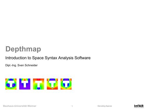
<strong>Depthmap</strong><br />
Introduction to Space Syntax Analysis Software<br />
Dipl.-Ing. Sven Schneider<br />
<strong>Bauhaus</strong>-Universität <strong>Weimar</strong> 1 Decoding Spaces
Download <strong>Depthmap</strong><br />
https://github.com/downloads/SpaceGroupUCL/<strong>Depthmap</strong>/<strong>Depthmap</strong>Setup1014.exe<br />
<strong>Bauhaus</strong>-Universität <strong>Weimar</strong> 2 Decoding Spaces
What is <strong>Depthmap</strong>?<br />
“It is a tool for topological analysis<br />
The analysis of layouts is achieved through the<br />
juxtaposition of graphs<br />
The graphs are analysed“<br />
Possible Types of Analysis are:<br />
• Convex Space Analysis<br />
• Axial Line Analysis<br />
• Segment Analysis<br />
• Visibility Graph Analysis (including single<br />
Isovists & Isovist Fields)<br />
• Agent Analysis<br />
<strong>Bauhaus</strong>-Universität <strong>Weimar</strong> 3 Decoding Spaces
Tutorial<br />
Download at:<br />
http://www.vr.ucl.ac.uk/depthmap/tutorials/<br />
<strong>Bauhaus</strong>-Universität <strong>Weimar</strong> 4 Decoding Spaces
<strong>Depthmap</strong> – User Interface<br />
Layer List<br />
Graphical<br />
Output<br />
Measures<br />
<strong>Bauhaus</strong>-Universität <strong>Weimar</strong> 5 Decoding Spaces
Importing Plans<br />
<strong>Depthmap</strong> is a pure Analysis Tool, it is not<br />
possible to draw plans!<br />
<strong>Depthmap</strong> can import 2-dimensional Plans.<br />
Fileformat working best is DXF (AutoCAD 2000<br />
Standard)<br />
After creating a new file (File New), you can<br />
import a plan (Map Import…)<br />
After importing, the plan is visible in the<br />
„Drawing Layers“ list.<br />
It is possible to import a number of plans. For<br />
each a new folder is added to the „Drawing<br />
Layers“ list.<br />
If your DXF File has different layers, these<br />
layers will be obtained in <strong>Depthmap</strong>. (This can<br />
be useful for analysing different design<br />
variants)<br />
<strong>Bauhaus</strong>-Universität <strong>Weimar</strong> 6 Decoding Spaces
Representations of space:<br />
Axial Lines, Convex Spaces und Isovists<br />
<strong>Bauhaus</strong>-Universität <strong>Weimar</strong> 7 Decoding Spaces
Convex Analysis<br />
It is not possible to detect Convex Spaces<br />
automatically!<br />
To make a Convex Analysis all the convex<br />
spaces have to be drawn „by hand“.<br />
For drawing a Convex Map in <strong>Depthmap</strong> it is<br />
useful to import a plan as a „template“.<br />
Then create a new map (Map New…) of the<br />
type „Convex Map“<br />
For drawing Click on the - icon<br />
and draw the convex spaces „above“ the plan<br />
After this you have to connect all the spaces<br />
which touch, by using the Join-tool<br />
Start the Analysis (Tools Axial / Convex /<br />
Pesh Run Graph Analysis Ok)<br />
<strong>Bauhaus</strong>-Universität <strong>Weimar</strong> 8 Decoding Spaces
Exercise: Convex Map<br />
Create new file<br />
Import the plan „<strong>InfAR</strong>_office.dxf“<br />
Create new Map (Map Type: Convex Map)<br />
Draw Convex Spaces<br />
Connect Convex Spaces<br />
Run Graph Analysis (Tools Axial / Convex /<br />
Pesh)<br />
Check Measures (Integration, Connectivity)<br />
<strong>Bauhaus</strong>-Universität <strong>Weimar</strong> 9 Decoding Spaces
Representations of space:<br />
Axial Lines, Convex Spaces und Isovists<br />
<strong>Bauhaus</strong>-Universität <strong>Weimar</strong> 10 Decoding Spaces
Axial Analysis<br />
Axial lines can be drawn by hand, as well as<br />
being generated automatically.<br />
After creating an Axial Map it can be analysed<br />
(Tools Axial / Convex / Pesh Run Graph<br />
Analysis Ok)<br />
The measures are the same as in the Convex<br />
Analysis<br />
<strong>Bauhaus</strong>-Universität <strong>Weimar</strong> 11 Decoding Spaces
Drawing Axial Maps<br />
Axial Maps can be drawn by hand, as well as<br />
generated automatically.<br />
To draw an Axial Map first a new map must be<br />
created (Map New… Axial Map)<br />
After clicking on the drawing icon<br />
Lines can be drawn.<br />
Axial<br />
Before drawing the Axial Map it is useful to<br />
import a plan as a „template“.<br />
Note: You can also import a „hand-drawn“ Map<br />
as an Axial Map. This way you can use your<br />
favourite CAD-Tool.<br />
<strong>Bauhaus</strong>-Universität <strong>Weimar</strong> 12 Decoding Spaces
Generating Axial Maps<br />
To automatically derive an Axial Map of a plan<br />
use Axial Map Tool<br />
This creates an All-Axial Line Map, means a<br />
map which evenly covers the open space with<br />
Axial Lines (e.g. Lines of sight).<br />
This All Line Map can be analyed: Tools <br />
Axial / Convex /Pesh Run Graph Analsyis<br />
By clicking on Tools Axial / Convex / Pesh <br />
Reduce to fewest line map the All-Line-Map<br />
can be converted to a fewest line map.<br />
<strong>Bauhaus</strong>-Universität <strong>Weimar</strong> 13 Decoding Spaces
Algorithm for Generating All Line Maps<br />
Taken from: Turner, Penn & Hillier (2005)<br />
<strong>Bauhaus</strong>-Universität <strong>Weimar</strong> 14 Decoding Spaces
All-Line-Map & Fewest-Line-Map<br />
Advantage:<br />
divides the space into many possible lines of<br />
sight ( higher resolution)<br />
Disadvantage:<br />
Number of lines depend on the number of<br />
vertices in the plan (can lead to uneven<br />
weightings of certain areas)<br />
Advantage:<br />
Number of lines does not depend on the<br />
number of vertices but on connecting convex<br />
spaces<br />
Disadvantage:<br />
Low resolution can lead to missing some<br />
important lines<br />
<strong>Bauhaus</strong>-Universität <strong>Weimar</strong> 15 Decoding Spaces
Overview: Graph Measures (Axial Maps, Convex Maps)<br />
Connectivity<br />
Integration<br />
Choice<br />
Number of elements, which are connected to a certain element<br />
Distance of an element to (all) other elements in relation<br />
to the number of elements in the complete system<br />
(To-Movement, Centrality)<br />
Indicates how often a element is passed, when calculating the<br />
shortest paths between elements<br />
(Through-Movement)<br />
Control / Controllability<br />
Entropy / Relativised Entropy<br />
Intensity<br />
<strong>Bauhaus</strong>-Universität <strong>Weimar</strong> 16 Decoding Spaces
Connectivity<br />
Connectivity measures the number of elements,<br />
which are connected to a certain element.<br />
Connectivity is a local measure, means it only<br />
takes into account the direct neighbours of an<br />
element. Connectivity = 3<br />
Connectivity in an All-Line-Map<br />
<strong>Bauhaus</strong>-Universität <strong>Weimar</strong> 17 Decoding Spaces
Integration (To-Movement, Closeness)<br />
Integration misst wie weit entfernt sich ein<br />
Element (bspw. Axial Line) in Relation zu<br />
(allen) anderen Elementen befindet.<br />
Integration is a global measure, means it only<br />
takes into account the relations of all element to<br />
an element.<br />
Depth = 13<br />
Der Wert wird in der Graphenanalyse auch als<br />
Zentralität bezeichnet.<br />
RRA, RA, Total Depth, Mean Depth sind<br />
Werte, die sich nur durch Umrechnung<br />
(Normalisierung, etc.) von Integration<br />
unterscheiden.<br />
Integration in an All-Line-Map<br />
<strong>Bauhaus</strong>-Universität <strong>Weimar</strong> 18 Decoding Spaces
Choice (Through-Movement, Betweeness)<br />
Choice gibt an wie oft ein Element passiert<br />
wird, wenn alle kürzesten Wege (von jedem<br />
Element zu jedem anderen) im Graphen<br />
durchlaufen werden.<br />
Shortest path<br />
between 2<br />
elements<br />
Der Wert wird in der Graphenanalyse auch als<br />
Durchgangspotential bezeichnet.<br />
Standardmäßig ist die Choice-Berechnung in<br />
<strong>Depthmap</strong> deaktiviert, da sie verhältnismäßig<br />
viel Rechenzeit erfordert.<br />
Choice in an All-Line-Map<br />
<strong>Bauhaus</strong>-Universität <strong>Weimar</strong> 19 Decoding Spaces
To-Movement & Through-Movement (Integration & Choice)<br />
Look at:<br />
http://www.slideboom.com/presentations/29255<br />
8/Intro-to-Space-Syntax_Day-1<br />
<strong>Bauhaus</strong>-Universität <strong>Weimar</strong> 20 Decoding Spaces
Exercise: Axial Analysis<br />
Create new file<br />
Import „Grasse.dxf“<br />
Create All-Line Map<br />
Run Graph Analysis (Tools Axial / Convex /<br />
Pesh)<br />
Check Measures (Connectivity, Integration,<br />
Choice)<br />
Reduce to fewest line map and analyse it.<br />
Compare the results with the All Line Map<br />
<strong>Bauhaus</strong>-Universität <strong>Weimar</strong> 21 Decoding Spaces
Scattergrams<br />
Scattergrams are used for examining<br />
correlations between different measures.<br />
A prominent example therefore is the<br />
correlation between integration and<br />
connectivity. The degree of correlation is called<br />
intelligibility.<br />
To visualize such correlations in <strong>Depthmap</strong><br />
switch the window to „Scatter Plot“:<br />
<strong>Bauhaus</strong>-Universität <strong>Weimar</strong> 22 Decoding Spaces
Scattergrams<br />
Measure plotted on the Y-Axis<br />
Measure plotted on the X-Axis<br />
Show regression line<br />
Show Coefficient of<br />
determination<br />
Select the<br />
Analysis<br />
Type<br />
<strong>Bauhaus</strong>-Universität <strong>Weimar</strong> 23 Decoding Spaces
Global and local analysis<br />
Global analysis takes into account the relations<br />
of all elements to all elements.<br />
Local analysis takes into account relations in a<br />
certain distance / radius of each element<br />
Global Integration<br />
Local Integration<br />
<strong>Bauhaus</strong>-Universität <strong>Weimar</strong> 24 Decoding Spaces
Global and local integration<br />
The radius defines to which depth from the<br />
original element other elements are taken into<br />
account for calculating its depth in the system.<br />
“Radius-3 integration presents a localised<br />
picture of integration, and we can therefore<br />
think of it also as local integration, while radiusn<br />
integration presents a picture of integration at<br />
the largest scale, and we can therefore call it<br />
global integration.” (Hillier, 1996)<br />
Note:<br />
Integration R1 = Connectivity<br />
4<br />
3<br />
2<br />
1<br />
Depth, R2 = 1+1+2+2 = 6<br />
Depth, R3 = 1+1+2+2+3+3 = 12<br />
Depth, Rn = 1+1+2+2+3+3+4+4 = 20<br />
<strong>Bauhaus</strong>-Universität <strong>Weimar</strong> 25 Decoding Spaces
Segment Analysis<br />
In this type of Analysis not the longest lines of<br />
sight are taken into account, but the segments<br />
between intersecting lines.<br />
For calculating the graph measures not the<br />
steps from one to another element are<br />
counted, but the angles between the<br />
intersecting points of the elements.<br />
Advantages of Segment Analysis:<br />
Axial Map<br />
- more detailed<br />
- better correlation with movement analysis<br />
(Hillier & Iida, 2005)<br />
Look at: http://www.slideboom.com/presentations/293659/Intro-to-Space-Syntax_Day-2<br />
Segment Map<br />
<strong>Bauhaus</strong>-Universität <strong>Weimar</strong> 26 Decoding Spaces
Creating Segment Maps<br />
Once you have a fewest line map, you can<br />
easily convert it to a segment map.<br />
Map Convert Active Map Select Segment<br />
Map as new Map Type<br />
<strong>Bauhaus</strong>-Universität <strong>Weimar</strong> 27 Decoding Spaces
Overview: Segment Analysis Measures<br />
Connectivity<br />
Number of elements, which are connected to a certain element (Note: in<br />
Segment-Analysis Connectivity is no indicator how many streets are<br />
connected to a street because it only takes into account the localised segment,<br />
connectivity mostly ranges between 2 and 6)<br />
Total Depth Angular Distance of an element to (all) other elements (To-Movement)<br />
Integration<br />
Angular Distance of an element to (all) other elements in relation<br />
to the number of elements in the complete system (To-Movement, Centrality)<br />
Choice<br />
Indicates how often a element is passed, when calculating the<br />
shortest paths between elements (Through-Movement)<br />
<strong>Bauhaus</strong>-Universität <strong>Weimar</strong> 28 Decoding Spaces
Total Depth (Segment Analysis)<br />
Total Depth in Segment Analysis does not take<br />
into account the steps from one segment to<br />
another, but angles between segmentintersections.<br />
0° means a step-depth of 0.0<br />
.<br />
.<br />
.<br />
45° means a step-depth of 0.5<br />
.<br />
.<br />
.<br />
90° means a step-depth of 1.0<br />
.<br />
.<br />
.<br />
td = 1.07 + 0.07 + 0.05 +<br />
1.1 + 0.06 + 0.1 + 0.47 +<br />
0.1 = 2,85<br />
<strong>Bauhaus</strong>-Universität <strong>Weimar</strong> 29 Decoding Spaces
Exercise – Segment Analysis<br />
Convert the Fewest Line Map of Grasse to a<br />
segment map (Map Convert Active Map <br />
Select Segment Map as new Map Type)<br />
Analyse the segment map (Tools Segment<br />
Run Segment Analysis)<br />
Compare the results to the ones of the Axial<br />
Analysis<br />
<strong>Bauhaus</strong>-Universität <strong>Weimar</strong> 30 Decoding Spaces
Representations of space:<br />
Axial Lines, Convex Spaces und Isovists<br />
<strong>Bauhaus</strong>-Universität <strong>Weimar</strong> 33 Decoding Spaces
Isovists<br />
By Clicking on the Isovist Icon<br />
create Isovists.<br />
you can<br />
You can create multiple Isovists and compare<br />
their properties by clicking on the different<br />
Isovist Measures in the Measures-List.<br />
For deleting Isovists, you have to switch on the<br />
„Editibale“-Mode in the Layer-List. (Note that<br />
sometimes <strong>Depthmap</strong> is buggy and does not<br />
delete Items properly!)<br />
<strong>Bauhaus</strong>-Universität <strong>Weimar</strong> 34 Decoding Spaces
Overview: Isovist Measures<br />
Area<br />
Perimeter<br />
Occlusivity<br />
Compactness<br />
Drift Magnitude<br />
Drift Angle<br />
Max Radial<br />
Min Radial<br />
Flächeninhalt des Sichtfeldes<br />
Umfang des Sichtfeldes<br />
Länge der „verdeckten“ Kanten<br />
Verhältnis von Area zu Perimeter in Relation zur idealen Kreisform<br />
Distanz vom Blickpunkt zum „Schwerpunkt“ des Isovist-Polygons<br />
Winkel des Vektors (Blickpunkt zu Schwerpunkt) zur X-Achse<br />
längster „Sichtstrahl“<br />
kürzester „Sichtstrahl“<br />
<strong>Bauhaus</strong>-Universität <strong>Weimar</strong> 35 Decoding Spaces
Isovist Measures - Examples<br />
circle square forest<br />
Area:<br />
Perimeter:<br />
Occlusivity:<br />
Compactness:<br />
400<br />
70.8<br />
0.0<br />
1.0<br />
400<br />
80<br />
0.0<br />
0.78<br />
298.1<br />
486.6<br />
416.5<br />
0.015<br />
<strong>Bauhaus</strong>-Universität <strong>Weimar</strong> 36 Decoding Spaces
Isovist Field<br />
“to quantify a whole configuration, more than a<br />
single isovist is required and he suggests that<br />
the way in which we experience a space, and<br />
how we use it, is related to the interplay of<br />
isovists”<br />
“Isovist fields record a single isovist property for<br />
all locations in a configuration”<br />
<strong>Bauhaus</strong>-Universität <strong>Weimar</strong> 37 Decoding Spaces
Isovist Field<br />
For creating an Isovist Field, you first have to<br />
set up a grid:<br />
In a Dialogbox you can adjust the gridsize. If<br />
your Model is scaled 1:1 then the unit is meter<br />
(m).<br />
After setting up the grid you have to „fill“ the<br />
open space<br />
Now you can create the visibility graph:<br />
Tools Visibility Make Visibility Graph<br />
<strong>Bauhaus</strong>-Universität <strong>Weimar</strong> 38 Decoding Spaces
Isovist Field<br />
Create a Isovist Field by clicking on<br />
Visibility Run Visibility Graph Analysis<br />
Click on „Calculate isovist properties“<br />
<strong>Bauhaus</strong>-Universität <strong>Weimar</strong> 39 Decoding Spaces
Exercise - Isovist Field<br />
Import „Campus.dxf“<br />
Set Grid to 2<br />
Fill the open space<br />
Calculate the isovist properties (Visibility <br />
Run Visibility Graph Analysis)<br />
<strong>Bauhaus</strong>-Universität <strong>Weimar</strong> 40 Decoding Spaces
Visibility Graph<br />
is a graph of mutually visible points in space<br />
In mathematical terms, a graph consists of two<br />
sets: the set of the vertices in the<br />
Graph and the set of edge connections joining<br />
pairs of vertices.<br />
The graph edges are undirected (that is, if v1<br />
can see v2 , then v2 can see v1 ).<br />
(see Turner et al, 2001)<br />
Schematic plan and visibility graph (from: Krämer & Kunze, 2005)<br />
<strong>Bauhaus</strong>-Universität <strong>Weimar</strong> 41 Decoding Spaces
Visibility Graph<br />
Create a Isovist Field by clicking on<br />
Visibility Run Visibility Graph Analysis<br />
Click on „Calculate visibility relationships“<br />
<strong>Bauhaus</strong>-Universität <strong>Weimar</strong> 42 Decoding Spaces
Overview: Visibility Graph Measures<br />
Connectivity<br />
gibt an wieviele Punkte im Raum mit einem Punkt verbunden<br />
sind (entspricht der Area eines Isovist)<br />
Integration<br />
gibt die durchschnittliche visuelle Distanz eines Punktes zu allen anderen<br />
Punkten an<br />
Clustering Coefficient<br />
Control /<br />
Controllability<br />
Entropy /<br />
Relativised Entropy<br />
Intensity<br />
<strong>Bauhaus</strong>-Universität <strong>Weimar</strong> 43 Decoding Spaces
Colour Range<br />
Sometimes you have to adjust the color-range<br />
for making differences in the results visible<br />
more clearly.<br />
<strong>Bauhaus</strong>-Universität <strong>Weimar</strong> 44 Decoding Spaces
Permeability / Visibility<br />
“Architecture might be defined as the process<br />
of giving definitions to otherwise undefined<br />
space by providing boundaries. The boundaries<br />
used to define spaces may be dynamic, like<br />
swinging doors, or static, like walls. They may<br />
be transparent, like glass windows, or opaque,<br />
like brick walls. Whatever the nature of the<br />
boundaries, once defined, they provide a<br />
structure that distinguishes inside and outside.<br />
Depending on the nature of the boundaries, the<br />
accessibility, i.e. permeability, and visibility<br />
between inside and outside can be controlled.<br />
Both permeability - where you can go - and<br />
visibility - what you can see - directly affects<br />
how buildings in general and houses in<br />
particular work spatially and how they are<br />
experienced by their occupants, inhabitants as<br />
well as visitors.”<br />
(Güney, 2007, p.2)<br />
<strong>Bauhaus</strong>-Universität <strong>Weimar</strong> 45 Decoding Spaces
De-connecting Links in an Axial Map<br />
When in an axial map 2 Lines intersect<br />
graphically, but are not connected in reality, as<br />
it is the case with bridges or tunnels, you have<br />
to de-connect the link(s) of the axial lines.<br />
Therefore press Unlink<br />
and click on the corresponding lines<br />
<strong>Bauhaus</strong>-Universität <strong>Weimar</strong> 46 Decoding Spaces
Overview: Isovist Measures<br />
Area<br />
Perimeter<br />
Occlusivity<br />
Compactness<br />
Drift Magnitude<br />
Drift Angle<br />
Max Radial<br />
Min Radial<br />
Flächeninhalt des Sichtfeldes<br />
Umfang des Sichtfeldes<br />
Länge der „verdeckten“ Kanten<br />
Verhältnis von Area zu Perimeter in Relation zur idealen Kreisform<br />
Distanz vom Blickpunkt zum „Schwerpunkt“ des Isovist-Polygons<br />
Winkel des Vektors (Blickpunkt zu Schwerpunkt) zur X-Achse<br />
längster „Sichtstrahl“<br />
kürzester „Sichtstrahl“<br />
<strong>Bauhaus</strong>-Universität <strong>Weimar</strong> 47 Decoding Spaces
Overview: Visibility Graph Measures<br />
Connectivity<br />
gibt an wieviele Punkte im Raum mit einem Punkt verbunden<br />
sind (entspricht der Area eines Isovist)<br />
Integration<br />
gibt die durchschnittliche visuelle Distanz eines Punktes zu allen<br />
anderen Punkten an<br />
Clustering Coefficient<br />
gibt an, wie viele der Punkte, die von einem Punkt aus gesehen<br />
werden können, sich gegenseitig sehen (kann als Maß für die<br />
Konvexität eines Isovisten gesehen werden)<br />
Control /<br />
Controllability<br />
gibt an wie kontrollierend bzw. kontrollierbar ein Element ist<br />
Entropy /<br />
Relativised Entropy<br />
gibt an wie geordnet ein System an einem bestimmten Punkt ist<br />
<strong>Bauhaus</strong>-Universität <strong>Weimar</strong> 48 Decoding Spaces
Clustering Coefficient<br />
“The clustering coeffcient is a measure of the<br />
extent to which all the lines of sight which<br />
could exist in the neighbourhood of a location in<br />
the visibility graph, do exist.<br />
If most of the locations visible from a location<br />
are mutually visible then c will approach 1. If<br />
many of the locations visible from a location are<br />
not mutually visible, then c will approach 0. “<br />
High Clustering Coefficient<br />
(nearly all of the locations<br />
inside the isovist are<br />
mutally visible)<br />
(O’Sullivan & Turner, 2001)<br />
Low Clustering Coefficient<br />
(just some locations inside<br />
the isovist are mutally<br />
visible)<br />
<strong>Bauhaus</strong>-Universität <strong>Weimar</strong> 49 Decoding Spaces
Clustering Coefficient<br />
(Examples)<br />
Red – High Clustering Coefficient<br />
Blue – Low Clustering Coefficient<br />
<strong>Bauhaus</strong>-Universität <strong>Weimar</strong> 50 Decoding Spaces
Step Depth<br />
Calculates the steps necessary to get from one<br />
single element to all the others<br />
Step Depth is available in every graph based<br />
analysis (Convex Spaces, Axial Maps, Visibility<br />
Graphs, Segment Maps)<br />
Shortcut: Strg+D<br />
Step Depth in a Visbility<br />
Graph from a node at the<br />
entrance of the flat<br />
<strong>Bauhaus</strong>-Universität <strong>Weimar</strong> 51 Decoding Spaces
Control / Controllability<br />
„control picks out visually dominant areas,<br />
whereas controllability picks out areas that<br />
may be easily visually dominated.<br />
…<br />
For control, each location is first assigned an<br />
index of how much it can see, the reciprocal of<br />
its connectivity. Then, for each point, these<br />
indices are summed for all the locations it can<br />
see. As should be obvious, if a location has a<br />
large visual field will pick up a lot of points to<br />
sum, so initially it might seem controlling.<br />
However, if the locations it can see also have<br />
large visual fields, they will contribute very little<br />
to the value of control.<br />
ci = Control of a node i<br />
kj = Connectivity of the nodes that node i<br />
is connected to<br />
So, in order to be controlling, a point must<br />
see a large number of spaces, but these<br />
spaces should each see relatively little. The<br />
perfect example of a controlling location is the<br />
location at the centre of Bentham's panopticon.”<br />
(Turner, 2004)<br />
<strong>Bauhaus</strong>-Universität <strong>Weimar</strong> 52 Decoding Spaces
Control / Controllability<br />
“Controllability (…) for a location it is simply<br />
the ratio of the total number of nodes up to<br />
radius 2 to the connectivity (i.e., the total<br />
number of nodes at radius 1).<br />
Applied to the panopticon example, it would<br />
seem to operate in a similar manner to control.<br />
Each of the cells is highly controllable, as the<br />
area of visual field is small compared to the<br />
area viewable from the centre to which it<br />
connects, while the centre is less controllable,<br />
as it links only to the cells within its field, and<br />
they add little extra visual field.” (Turner, 2004)<br />
“Controllable spaces, on the other hand, are<br />
locations that can be easily seen from other<br />
locations but themselves cannot see much.”<br />
(Güney, 2007)<br />
Controllability = Connectivity R2 / Connectivity (R1)<br />
=<br />
/<br />
das was man auf den „zweiten Blick“ sieht<br />
/<br />
das was man auf den ersten Blick sieht<br />
Wenn Controllability hoch ist, ist der Zugang zu<br />
entsprechenden Punkt im Raum sehr einfach und<br />
vice versa.<br />
<strong>Bauhaus</strong>-Universität <strong>Weimar</strong> 53 Decoding Spaces
Control / Controllability<br />
„However, the panopticon is, of course, a<br />
contrived example. In reality, some spaces can<br />
be both controllable and controlling, and others<br />
uncontrollable and uncontrolling. It would seem<br />
an interesting avenue of research to see if<br />
anything further can be made from these<br />
measures, for example, to look at locations<br />
where crimes are committed, where a robber<br />
will want to control the victim, but at the same<br />
time be uncontrollable by the forces of law and<br />
order.”<br />
(Turner, 2004)<br />
Control<br />
Controllability<br />
<strong>Bauhaus</strong>-Universität <strong>Weimar</strong> 54 Decoding Spaces
Adding measures in <strong>Depthmap</strong><br />
Click on Attributes Add Column type in a<br />
name right-click on the new measure in the<br />
measures-list and chose edit<br />
http://www.vr.ucl.ac.uk/depthmap/scripting/salascript.pdf<br />
<strong>Bauhaus</strong>-Universität <strong>Weimar</strong> 61 Decoding Spaces
Integration in Segment Maps<br />
Global Integration<br />
Local Integration<br />
(Bsp. R750)<br />
value("T1024 Node Count")/value("T1024<br />
Total Depth")<br />
(value("T1024 Node Count R750<br />
metric")^2))/(value("T1024 Total Depth R750<br />
metric")<br />
Integration-Choice<br />
Combination<br />
(value("T1024 Node Count")/value("T1024<br />
Total Depth"))*(log(value("T1024<br />
Choice")+2))<br />
<strong>Bauhaus</strong>-Universität <strong>Weimar</strong> 62 Decoding Spaces
Agent Analysis<br />
“In agent-based analysis virtual `people' (called<br />
agents) are released into the environment, and<br />
make decisions on where to move within it. The<br />
agents require a visibility graph in order for<br />
them to have vision of the environment.<br />
…<br />
The original agents from Turner and Penn<br />
(2002) simply select a destination at random<br />
from their field of view, take a few steps<br />
towards, before selecting another destination.<br />
…<br />
The analysis may be performed accurately,<br />
counting agents passing through gates just as<br />
people can be measured passing through gates<br />
in the real world.<br />
…<br />
If agents are programmed to move towards<br />
occluding edges rather than open space, then<br />
their movement patterns tend to be drawn<br />
between the lines joining those occluding<br />
edges. Since the occluding edges in an<br />
environment are simply the concave corners<br />
within it, the agents start to embody the axial<br />
system with their movement.”<br />
(Turner, 2007)<br />
<strong>Bauhaus</strong>-Universität <strong>Weimar</strong> 63 Decoding Spaces
Agent Analysis in <strong>Depthmap</strong><br />
Tools Agent Analysis Run Agent Analysis<br />
(only available after a visibility graph is made)<br />
<strong>Bauhaus</strong>-Universität <strong>Weimar</strong> 64 Decoding Spaces
New: Space Syntax in Grasshopper<br />
See: “The parametric exploration of spatial properties –<br />
Coupling parametric geometry modeling and the graphbased<br />
spatial analysis of urban street networks”<br />
(Schneider, Bielik & König, 2012)<br />
Figure 1. Designing is a cyclical process where artifacts are<br />
created with the help of design tools (see Gänshirt, 2007)<br />
Figure 2: Screenshot of Rhino, Grasshopper and the new<br />
Spatial Analysis Components<br />
<strong>Bauhaus</strong>-Universität <strong>Weimar</strong> 65 Decoding Spaces
New: Space Syntax in Grasshopper<br />
Figure 3: Modular concept of the spatial analysis framework for Grasshopper<br />
Figure 4. The ConvertToSegmentMap Component<br />
converts geometric structures into segment maps<br />
Figure 5. Converting a segment map into a graph (for<br />
details see Hillier & Iida, 2005)<br />
<strong>Bauhaus</strong>-Universität <strong>Weimar</strong> 66 Decoding Spaces
New: Space Syntax in Grasshopper<br />
Coupling Analysis & Modeling offers 2<br />
important advantages:<br />
1. Effectively comparing design variants<br />
2. Using analyis results as parameters for the<br />
parametric model<br />
Figure 7. Relating betweenness (choice) to<br />
the width of streets<br />
Figure 6. Three design variants deriving from a simple parametric<br />
model, analysed in terms of betweenness (first row) and centrality<br />
(second row)<br />
Figure 8. Relating centrality (integration) to the<br />
height of buildings<br />
<strong>Bauhaus</strong>-Universität <strong>Weimar</strong> 67 Decoding Spaces
Space Syntax Mailinglist<br />
<strong>Bauhaus</strong>-Universität <strong>Weimar</strong> 68 Decoding Spaces


