Lecture XI
Lecture XI
Lecture XI

You also want an ePaper? Increase the reach of your titles
YUMPU automatically turns print PDFs into web optimized ePapers that Google loves.
Particle Physics 2011<br />
Luis Anchordoqui<br />
Thursday, November 17, 2011
Radiative Corrections<br />
As a rule ☛ size of radiative corrections to a given process is<br />
determined by discrepancy between various mass & energy scales involved<br />
For a wide class of low-energy and<br />
-boson observables<br />
dominant effects originate entirely in gauge boson propagators<br />
➊●⦁<br />
●⦁<br />
➋ ∆ρ<br />
●⦁<br />
➌<br />
●⦁<br />
➍<br />
(oblique corrections)<br />
and can be parametrized in terms of 4 electroweak parameters:<br />
∆α<br />
Z<br />
∆α, ∆ρ, ∆r, and ∆κ<br />
determines running fine structure constant at<br />
α(m Z )/α = (1 − ∆α) −1<br />
Z<br />
boson scale<br />
measures quantum corrections of NC/CC amplitudes at low energy<br />
∆r embodies non-photonic corrections to muon lifetime<br />
∆κ<br />
controls effective weak mixing angle<br />
that occurs in ratio of<br />
Thursday, November 17, 2011<br />
sin 2 ¯θw = sin 2 θ w (1 + ∆κ)<br />
Zf ¯f<br />
vector and axial-vector couplings<br />
i.e. c f V /cf A =1− 4|Q f | sin 2 ¯θw
Chess Notation<br />
Today’s class ☛ intro to theory of electroweak radiative corrections<br />
and its role in testing SM, predicting top mass, constraining Higgs mass,<br />
and searching for deviations that may signal presence of new physics<br />
Implementing such a program<br />
can be first formulated from point of view of experimentalist<br />
Introducing notation ☛<br />
sin 2 θ w = s 2 =1− c 2 , m 2 W ≡ w, m 2 Z ≡ z<br />
Electroweak theory predicts at Born level that:<br />
w<br />
z<br />
=1− s2<br />
♜<br />
σ(ν µ e)<br />
σ(¯ν µ e) = 3 − 12s2 + 16s 4<br />
♚<br />
1 − 4s 2 + 16s 4<br />
πα 1<br />
√<br />
2 GF<br />
w = s2<br />
♟<br />
Γ(Z → f ¯f)<br />
m Z<br />
= α 3 C F<br />
((c f V )2 +(c f A )2)<br />
♝<br />
A LR ≃ A τ ≃<br />
[ 4<br />
3 A FB<br />
] 1/2<br />
≃ 2(1 − 4s 2 )<br />
♛<br />
Thursday, November 17, 2011
Chessboard<br />
Chess Eqs. represent incomplete list of experiments<br />
capable of measuring sin 2 θ w<br />
Validity of SM requires that each measurement yields same value of s 2<br />
〡<br />
Ratio of<br />
ν µ<br />
scattering on left- and right-handed electrons<br />
which is a function of<br />
sin 2 θ w<br />
only ☛<br />
♚<br />
〢<br />
Measurement of weak boson masses ☛<br />
♜<br />
〣<br />
m W ,α G F ♟<br />
Combination of , and as determined by muon lifetime ☛<br />
ⅠⅤ<br />
Ⅴ<br />
Partial widths of<br />
with vector<br />
and color factor<br />
Z<br />
into a fermion pair<br />
and axial coupling<br />
c f V<br />
and<br />
c f A<br />
C F = 3 (1) for quarks (leptons) ☛<br />
Various asymmetries measured at Z-factories ☛ ♛<br />
♝<br />
Thursday, November 17, 2011
Corrections to<br />
Z<br />
propagator<br />
After inclusion of<br />
O(α)<br />
corrections<br />
sin 2 θ w values obtained from different methods will no longer be same<br />
ple,<br />
because<br />
the diagram<br />
radiative example, the corrections diagram modify chess eqs. in different ways<br />
E.G.<br />
diagram ☛<br />
Z<br />
W W<br />
modifies -channel (5.5.92)<br />
(5.5.92)<br />
W (5.5.92)<br />
propagator measured by ♚<br />
W<br />
fies<br />
It<br />
the<br />
does<br />
t-channel<br />
not It does<br />
Z propagator<br />
-- not, however, contribute<br />
measured<br />
-- contribute to O(α) shifts in<br />
by (5.5.87); see<br />
to the W, Z masses<br />
also (5.1.27).<br />
shifts in masses<br />
f<br />
W<br />
es not, however, contribute to O(α) shiftsf<br />
in the W, Z masses<br />
Z<br />
W<br />
example, the diagram<br />
f<br />
+ + +<br />
W. . .<br />
W<br />
W<br />
H<br />
+ + + . . .<br />
(5.5.93)<br />
+ + + . . .<br />
W<br />
W<br />
modifies the t-channel Z propagator measured by (5.5.87); see also (5.1.27).<br />
modifies It does not, the t-channel however, contribute Z propagator O(α) measured shiftsby in (5.5.87); the W, Zsee masses also (5.1.27).<br />
Z<br />
Z<br />
W<br />
W<br />
Z<br />
Z<br />
Z<br />
+ + + . . .<br />
f<br />
f<br />
W<br />
t<br />
(5.5.93)<br />
(5.5.93)<br />
f<br />
W<br />
H<br />
W<br />
(5.5.94)<br />
which yield an improved sin 2 θ w<br />
sin 2 value θvia w (5.5.88). value There viais no♜<br />
real mystery (5.5.94)<br />
which here. yield Afteran inclusion improved of sin O(α) 2 θ w contributions value via (5.5.88). in Eqs. There (5.5.87)–(5.5.91), is no real mystery they<br />
which yield an improved<br />
Thursday, November 17, 2011<br />
W<br />
H<br />
O(α)<br />
W, Z
Weinberg Angle<br />
Experimentalist has to make a choice and define Weinberg angle to<br />
All other experiments should be reformulated in terms of preferred<br />
What this choice should be is no longer a matter of debate<br />
we will define<br />
sin 2 θ w<br />
in terms of physical masses of weak bosons<br />
O(α)<br />
s 2<br />
i.e.<br />
sin 2 θ w ≡ 1 − m2 W<br />
m 2 Z<br />
=0.23122(15) ☎<br />
This choice is particularly useful in that one can estimate<br />
radiative corrections in terms of renormalization group<br />
which has been previously introduced<br />
O(α)<br />
corrections can be qualitatively understood<br />
in terms of loop corrections to vector-boson propagators<br />
<br />
and<br />
<br />
A most straightforward test of theory is now obtained<br />
by fixing<br />
sin 2 θ w<br />
in terms of measured weak boson masses<br />
and verifying that its value coincides with other measurements of<br />
θ w<br />
Thursday, November 17, 2011
Free Parameters<br />
All UV divergences in QED can be absorbed in two parameters:<br />
α<br />
and<br />
m e<br />
List of parameters to be fixed by experiment in electroweak theory includes<br />
α, m W ,m Z ,m H ,m f<br />
<br />
g, g ′ , λ, µ, Y f<br />
weak mixing angle does not appear in list of parameters:<br />
its value is automatically determined by via ☎<br />
Traditionally ☛ SM Lagrangian is determined in terms of<br />
There is in fact a direct translation between sets and ☕<br />
☕<br />
m W ,m Z<br />
g 2 = e 2<br />
z<br />
z − w<br />
g ′2 = e 2 z w<br />
λ = e 2<br />
zm 2 H<br />
8w(z − w)<br />
Y f = e 2<br />
zm 2 f<br />
2w(z − w)<br />
Thursday, November 17, 2011
Y f = e 2<br />
2w(z − w) . (5.5.101)<br />
Electromagnetic Radiative Corrections<br />
As an example we will show how the relation (5.5.89) zm<br />
Show how relation ♟ is calculated to O(α)<br />
2 is calculated to<br />
Y<br />
O(α) in terms of the weak angle θ<br />
θ<br />
w defined by f = e<br />
(5.5.88). 2 f<br />
example ☛<br />
The origin of the<br />
relation in terms (5.5.89) of weak is the angle muon’s lifetime w defined which, to by leading ♜ order, is given by<br />
Origin of relation the diagram ♟ is lifetime ☛ to leading order is given by diagram<br />
µ<br />
and<br />
f<br />
H<br />
λ = e 2<br />
8w(z − w) , (5<br />
2w(z − w) . (5<br />
As an example we will show how the relation (5.5.89) is calcula<br />
O(α) in terms of the weak angle θ w defined by (5.5.88). The origin<br />
relation (5.5.89) is the muon’s lifetime which, to leading order, is gi<br />
the diagram<br />
Γ (0)<br />
µ = W<br />
Γ (0)<br />
µ = W<br />
(5.5.102)<br />
(5<br />
In Fermi theory In Fermi ☛ theory, electromagnetic radiative corrections must be included to<br />
must be included obtain the to result obtain to O(α). result Symbolically, to O(α)<br />
Symbolically Γ (1)<br />
where<br />
In Fermi theory, electromagnetic radiative corrections must be inclu<br />
obtain the result to O(α). Symbolically,<br />
µ = G F<br />
√ [1 + photonic Γ (1)<br />
µ = G F<br />
corrections] , (5.5.103)<br />
2<br />
Γ (1)<br />
√<br />
2<br />
[1 + photonic corrections] , (5<br />
µ = G F<br />
√ [1 + photonic corrections]<br />
2<br />
where<br />
<br />
where<br />
photonic corrections = + . . . (5<br />
photonic corrections =<br />
photonic corrections = + . . . (5.5.104)<br />
Thursday, November 17, 2011
Electroweak Radiative Corrections<br />
]<br />
[<br />
Γ (1)<br />
µ = e2 + box<br />
1 + photonic corrections<br />
electroweak In electroweak theory, on thetheory<br />
other hand,<br />
8s 2 c 2 z<br />
where<br />
+ propagator<br />
[<br />
[<br />
In electroweak Γ (1) theory, on the other<br />
Γ (1) hand,<br />
µ = e2<br />
+ vertex<br />
µ = e2<br />
1 + photonic corrections<br />
8s 2 c 2 z<br />
f ]<br />
[<br />
8s 2 c 2 1 + photonic corrections<br />
z<br />
Γ (1)<br />
µ = e2 + propagator<br />
+ box<br />
1 + photonic corrections<br />
8s 2 c 2 z+ vertex<br />
propagator<br />
(5.5.105)<br />
= +<br />
where + propagator ♬<br />
]<br />
+ box+ propagator<br />
(5.5.105)<br />
+ vertex<br />
+ vertex f<br />
ere<br />
]<br />
]<br />
+ box<br />
H<br />
propagator + = box +<br />
f<br />
t<br />
where<br />
where<br />
+<br />
propagator = +<br />
f<br />
t<br />
H<br />
propagator = +<br />
+<br />
H<br />
+<br />
+<br />
H<br />
In electroweak theory, on the other + vertex hand,<br />
+. . .<br />
vertex = + . . .<br />
+. . . (5.5.106)<br />
+. . . (5.5.106) Z<br />
and<br />
vertex = + . . . (5.5.107)<br />
vertex = + . . .<br />
vertex = + . . . (5.5.107) box = + . . .<br />
Thursday, November 17, 2011<br />
Z<br />
and<br />
and<br />
Z<br />
Equating (5.5.103) and (5.5.105) we obtain<br />
W<br />
box = + . . .<br />
t<br />
t<br />
+. . .
Electroweak Model at Born Level@<br />
e threshold for producing charmed par-<br />
. Above the threshold for all five quark<br />
1 as predicted. These measurements conuark,<br />
because R = 11 would be reduced<br />
3<br />
e color.<br />
with<br />
ified when interpreted in the context of<br />
the (leading order) process e + e − → q¯q.<br />
grams where the quark and/or antiquark<br />
<br />
Equating and ♬ we obtain G F = πα<br />
Before discussing status of measurements of<br />
σ e + e − →q ¯q<br />
α = e2<br />
4π<br />
∆r =∆α − c2<br />
to leading order ☛ ∆r =0<br />
using<br />
σ e + e − →µ + µ − (3.5.86)<br />
coupling α,<br />
1<br />
√ (1 + ∆r)<br />
2 ws2 ∆r ☛<br />
s 2 ∆ρ +∆ rem<br />
note that<br />
m W = gv<br />
2 = g<br />
2 √ 2 λ m H and m Z = m W<br />
cos θ w<br />
♒<br />
<br />
♒<br />
(3.5.87)<br />
reduces to Born relation<br />
♟<br />
Thursday, November 17, 2011
nate this quantity. We specifically isolated the fermions which are responsible<br />
the electroweak radiative corrections are gathered in ∆r. Notation (5.5.110)<br />
for Dominant Terms<br />
recognizes the running the fact of αthat from in the theOMS muon scheme, to thevacuum Z mass, polarization loops dominate<br />
this quantity. We specifically isolated the fermions which are<br />
Electroweak radiative corrections are gathered in ∆r<br />
responsible<br />
for the running of α from the muon to the Zf<br />
mass,<br />
We specifically isolated fermions which are responsible for running of<br />
∆α = ∑ f<br />
(5.5.111)<br />
f<br />
∆α = ∑ f<br />
(5.5.111)<br />
as well as the third generation, heavy quark diagram<br />
as well as third generation heavy quark diagram<br />
as well as the third generation, heavy quark diagram<br />
∆ρ = t<br />
W<br />
∆ρ =<br />
W<br />
t<br />
(5.5.112)<br />
(5.5.112)<br />
∆ rem<br />
Other contributions are small and are grouped in remainder<br />
Other contributions are small in the OMS scheme and are grouped in the<br />
To “remainder” Other can extent contributions imagine ∆ rem that . summing are ∆small rem the inis the series small OMS ☛ one scheme and can areimagine grouped insumming the series<br />
“remainder” Before discussing ∆ rem . the status of measurements of ∆r, we make several comments.<br />
Before To discussing leading order the status ∆r = of0 measurements of ∆r, we make several comments.<br />
+<br />
and, using (3.5.87) and (2.4.88), (5.5.109)<br />
+ . . .<br />
reduces to<br />
To<br />
the<br />
leading<br />
Born<br />
order<br />
relation<br />
∆r =<br />
(5.5.89).<br />
0 and, using<br />
The full<br />
(3.5.87)<br />
order<br />
and<br />
α calculation<br />
(2.4.88), (5.5.109)<br />
of ∆r will<br />
reduces to the Born relation (5.5.89). The full order α calculation of ∆r will<br />
not be presented here. We have attempted to describe the full formalism in<br />
not be presented here. We have attempted to describe the full formalism in (5.5.113)<br />
by a relatively replacement accessible (1 way + elsewhere. ∆r) →<br />
a relatively accessible way elsewhere. 23 (1 23 To− the∆r) extent −1<br />
by the replacement (1 + ∆r) →<br />
that ∆<br />
To(1the extent ∆r) −1 that in (5.5.109).<br />
in<br />
∆ rem ♒ is small, one<br />
rem is small, one<br />
Thursday, November 17, 2011
∆ρ<br />
recognizes the fact that in the OMS scheme, vacuum polarization ∆α = loops ∑ dominate<br />
this quantity. We specifically isolated the fermions which are responsible<br />
f<br />
for the running of α from the muon to the Z mass,<br />
We already discussed running of<br />
α<br />
from small lepton masses to<br />
f<br />
m Z<br />
as well as the third generation, heavy quark diagram<br />
∆α = ∑ (5.5.111)<br />
f<br />
t<br />
Other large contribution<br />
∆ρ<br />
which represents loop ☛<br />
as well as the third generation, heavy quark diagram<br />
∆ρ =<br />
W<br />
Its value is given by<br />
∆ρ = α 4π<br />
with<br />
N C =3<br />
z<br />
ω(z − ω) N C|U tb | 2 [ m 2 t F (m 2 t ,m 2 b)+m 2 bF (m 2 b,m 2 ]<br />
t ) Other contributions are small in the OMS scheme and are grouped in the<br />
F (m 2 1,m 2 2)=<br />
∆ρ =<br />
where is number of colors and U tb is CKM matrix element<br />
Thursday, November 17, 2011<br />
|U tb | 2 ≃ 1<br />
t<br />
is our primary focus here<br />
Other contributions are small in the OMS scheme<br />
(5.5.112)<br />
“remainder” W ∆ rem .<br />
Before discussing the status of measurements of ∆<br />
ments. To leading order ∆r = 0 and, using (3.5.87<br />
reduces to the Born relation (5.5.89). The full order<br />
<br />
not be presented here. We have attempted to descr<br />
a relatively accessible way elsewhere. 23 To the exten<br />
“remainder” ∆ rem .<br />
Before discussing ∫ the status of measurements 1<br />
[ of ∆r, we make several<br />
dx x ln m 2 1(1 − x)+m 2 ]<br />
comments.<br />
To leading order ∆r = 0 and, using (3.5.87) and (2.4.88), (5.5.109)<br />
reduces to the Born relation (5.5.89). 23 F. The Halzen fulland order D. αA. calculation Morris, Phys.<br />
2x of ∆r Lett. will ☢B 237, 107 (199<br />
not be presented here. 0 We have F. attempted Halzen and to describe B. A. Kniehl, the full Nucl. formalism Phys. Bin<br />
353, 567 (199<br />
a relatively accessible way elsewhere. M. L. 23 Stong, To thePhys. extent Lett. thatB ∆277, rem is 503 small, (1992); oneF. Halzen, B.<br />
Z. Phys. C 58, 119 (1993); M. C. Gonzalez-Garcia, F. Halze<br />
23 F. Halzen and D. A. Morris, Phys. Lett. B 237, 107 (1990); Part. World 2, 10 (1991);<br />
Lett. 322, 233 (1994).<br />
F. Halzen and B. A. Kniehl, Nucl. Phys. B 353, 567 (1991); F. Halzen, P. Roy and<br />
M. L. Stong, Phys. Lett. B 277, 503 (1992); F. Halzen, B. A. Kniehl and M. L. Stong,<br />
174
Fingeprints of Electroweak theory<br />
e third generation, heavy quark diagram<br />
Diagram<br />
In QED<br />
ibutions are small in the OMS scheme and are grouped in the<br />
only equal mass fermions and antifermions appear in neutral photon loops<br />
∆ rem .<br />
and diagrams of this type are not possible<br />
iscussing the status of measurements of ∆r, we make several comleading<br />
Rewrite order<br />
∆r and = 0 and, ☢<br />
using form (3.5.87) and (2.4.88), (5.5.109)<br />
he Born relation (5.5.89). The full<br />
∆ρ = G order [ α calculation of ∆r ]<br />
F<br />
m 2 t + m 2 b − 2m2 will<br />
ented here. We have attempted to describe the full formalism in b m2 t<br />
accessible way elsewhere. 23 To the extent that ∆ rem is small, one<br />
m 2 t /z<br />
∆ρ =<br />
≃<br />
4π<br />
G F<br />
4π m2 t ≃ 3α<br />
16π<br />
m 2 t − m 2 b<br />
1 m 2 t<br />
c 2 s 2 z<br />
ln m2 t<br />
m 2 b<br />
contribution to an observable is forbidden in QED and QCD<br />
where virtual particle effects are suppressed by inverse powers of their masses<br />
⌚ embodies this 174 requirement because ɛ =0 for photon loops<br />
Conversely ☛ appearance of<br />
W<br />
t<br />
has important property that<br />
m 2 t /z<br />
term<br />
(5.5.112)<br />
and D. A. Morris, Phys. Lett. B 237, 107 (1990); Part. World 2, 10 (1991);<br />
d B. A. Kniehl, Nucl. Phys. B 353, 567 (1991); F. Halzen, P. Roy and<br />
Phys. Lett. B 277, 503 (1992); F. Halzen, B. A. Kniehl and M. L. Stong,<br />
, 119 (1993); M. C. Gonzalez-Garcia, F. Halzen and R. A. Vazquez, Phys.<br />
233 (1994).<br />
Thursday, November 17, 2011<br />
defining<br />
m t = m b + ɛ<br />
☛<br />
∆ρ ≃ G F<br />
3π 2 ɛ<br />
❃<br />
is a characteristic feature of electroweak theory<br />
⌚
We are now ready to illustrate that ...<br />
<br />
<br />
<br />
We first determine experimental value of<br />
Using<br />
G F<br />
√<br />
2<br />
=<br />
g2<br />
8m 2 W<br />
and<br />
∆r exp ≃ 1 − (37.281 GeV) 2<br />
We next recall<br />
Crucial point is that<br />
O(α)<br />
∆α ≃ 1 −<br />
∆r exp ≠∆α<br />
∆r<br />
from<br />
e = g sin θ w<br />
♒<br />
z<br />
ω(z − ω) ≃ 0.035<br />
α(0)<br />
α(m 2 Z ) ≃ 1 − 128<br />
137 ≃ 0.066<br />
(◬ ≠⌛)<br />
SM relation requires a non-vanishing<br />
value of<br />
∆ρ ≠0<br />
◬<br />
⌛<br />
∆ρ<br />
<br />
<br />
Using ❃ we obtain that<br />
∆ρ =0.0086<br />
and yields<br />
(∆r) calculated =∆α − c2<br />
∆ρ =0.037<br />
s2 in agreement with experimental value<br />
We leave it as an exercise to insert errors into calculation<br />
and show that argument survives a straightforward statistical analysis<br />
Thursday, November 17, 2011
to insert errors into the calculation and show that our argument survives a<br />
straightforward Constrains statistical analysis. on Higgs Mass<br />
The Higgs particle makes a contribution to ∆r:<br />
Higgs particle makes a contribution to<br />
∆r<br />
∆h =<br />
∆h =<br />
W<br />
H<br />
= 11α<br />
48π<br />
48π<br />
1<br />
1<br />
c ln m2 H<br />
2 z . (5.5.121)<br />
c 2 ln m2 H<br />
z<br />
From<br />
we obtain that<br />
From (5.3.59) we obtain that ∆h < 0.0006, a contribution too small to<br />
contribution be sensed too small by the simple to be analysis sensed presented by simple above. analysis The quantity presented ∆r is in above<br />
principle Quantity sensitive ∆r is to in theprinciple Higgs mass. sensitive More sophisticated to Higgs analyses mass which<br />
include the dominant O(α 2 ) corrections are now yielding weak, but definite,<br />
constraints on the value of m H .<br />
Other measurements support the electroweak model’s radiative correction<br />
associated<br />
program<br />
with the<br />
is<br />
t¯b<br />
however<br />
loop ∆ρ.<br />
far<br />
Recall<br />
from<br />
that charged<br />
complete<br />
weak currents couple with<br />
problem strength Gcan F , while be quantified neutral currents by couple rewriting as ρG F ; ◬ see and (5.1.10) and as(5.1.23).<br />
Radiative corrections predicted by SM have successfully confronted experiment<br />
Using<br />
Z<br />
∆r exp = F (m W 176 ,m t ,m H )<br />
-pole measurements of SLD and LEP1<br />
electroweak radiative corrections are evaluated<br />
to predict masses of top quark and<br />
Thursday, November 17, 2011<br />
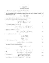
114.4 GeV
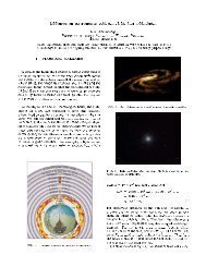
(m W ,m t )<br />
plane<br />
July 2008<br />
80.5<br />
LEP2 and Tevatron (prel.)<br />
LEP1 and SLD<br />
68% CL<br />
m W<br />
[GeV]<br />
80.4<br />
80.3<br />
!"<br />
m H<br />
[GeV]<br />
114 300 1000<br />
150 175 200<br />
m t<br />
[GeV]<br />
m t ,m W<br />
Contour curves of 68% CL in (<br />
) plane<br />
for<br />
Figure<br />
direct<br />
5.5: Contour<br />
measurements<br />
curves of 68% CL<br />
and<br />
in the<br />
indirect<br />
(m t ,m W )<br />
determinations<br />
plane for direct measurements<br />
and the indirect determinations.<br />
mThe band shows the correlation<br />
Band shows correlation between W and m expected in SM<br />
between m W and m t expected in the standard model. t<br />
Thursday, November 17, 2011
Neutrino Oscillation<br />
Convincing experimental evidence exists<br />
for oscillatory transitions<br />
ν α ⇋ ν β<br />
Simplest and most direct interpretation of atmospheric data<br />
is that of muon neutrino oscillations<br />
Evidence of atmospheric ν µ disappearing is now at > 15σ<br />
most likely converting to ν τ<br />
Angular distribution of contained events shows that<br />
for<br />
deficit comes mainly from<br />
E ν ∼ 1 GeV<br />
between different neutrino flavors<br />
L atm ∼ 10 2 − 10 4 km<br />
These results have been confirmed by KEK-to-Kamioka (K2K) experiment<br />
which observes disappearance of accelerator ν µ at a distance of<br />
Data collected by the Sudbury Neutrino Observatory (SNO)<br />
in conjunction with data from Super-Kamiokande (SK)<br />
show that solar ν e convert to ν µ or ν τ with CL of more than<br />
7σ<br />
250 km<br />
KamLAND Collaboration has measured flux of ν e from distant reactors<br />
and find that ν e disappear over distances of about 180 km<br />
All these data suggest that neutrino eigenstates that travel through space<br />
are not flavor states that we measured through weak force<br />
but rather mass eigenstates<br />
Thursday, November 17, 2011
Lepton Flavor Mixing<br />
|ν α 〉 |ν i 〉<br />
U<br />
Flavor eigenstates and mass eigenstates<br />
are related by a unitary transformation<br />
|ν α 〉 = ∑ i<br />
U αi |ν i 〉 ⇔ |ν i 〉 = ∑ α<br />
(U † ) iα |ν α 〉 = ∑ α<br />
(i.e. mixing matrix)<br />
U ∗ αi|ν α 〉<br />
with<br />
U † U = I, i.e., ∑ U αi Uβi ∗ = δ αβ and<br />
i<br />
For antineutrinos one has to replace U αi by<br />
i.e.<br />
|¯ν α 〉 = ∑ Uαi|¯ν ∗ i 〉<br />
i<br />
⨸<br />
∑<br />
i<br />
Uαi<br />
∗<br />
U αi U ∗ αj = δ ij<br />
♁<br />
Number of parameters of an unitary matrix<br />
It is easy to see that relative phases of n 2<br />
is<br />
neutrino states<br />
can be redefined such that<br />
n × n<br />
2n − 1<br />
(n − 1) 2<br />
1<br />
2 n(n − 1) weak mixing angles of an n<br />
and<br />
1<br />
2<br />
Thursday, November 17, 2011<br />
For these it is convenient to take:<br />
(n − 1)(n − 2)<br />
CP<br />
-violating phases<br />
2n<br />
independent parameters are left<br />
-dimensional rotation
Hamiltonian Mechanics<br />
⚈<br />
Being eigenstates of mass matrix ☛ states<br />
|ν i 〉<br />
(i.e. they have the time dependence)<br />
are stationary states<br />
|ν i (t)〉 = e −iE it |ν i 〉<br />
where<br />
with<br />
E ≈ p<br />
E i =<br />
√<br />
☛ here it is assumed that<br />
p 2 + m 2 i ≈ p + m2 i<br />
2p ≈ E + m2 i<br />
2E<br />
is total neutrino energy<br />
neutrinos are stable<br />
<br />
⚈<br />
A pure flavor state<br />
|ν α 〉 = ∑ i<br />
U αi |ν i 〉 present at t =0<br />
develops with time into state<br />
|ν(t)〉 = ∑ i<br />
U αi e −iE it |ν i 〉 = ∑ i,β<br />
U αi U ∗ βie −iE it |ν β 〉<br />
Thursday, November 17, 2011
Transition Amplitude<br />
Time dependent transition amplitude<br />
for transition from flavor<br />
ν α<br />
to flavor<br />
ν β<br />
is<br />
A(ν α → ν β ) ≡〈ν β |ν(t)〉 = ∑ i<br />
U αi U ∗ βie −iE it<br />
<br />
= ∑ i,j<br />
U αi δ ij e −iE it (U † ) jβ<br />
with D ij = δ ij e −iE it<br />
(diagonal matrix)<br />
= (UDU † ) αβ<br />
An equivalent expression for transition amplitude is obtained by<br />
inserting into and extracting an overall phase factor e −iEt<br />
A(ν α → ν β ,t) = ∑ i<br />
U αi Uβi ∗ e − im2 i t<br />
2E<br />
= ∑ i<br />
U αi Uβi ∗ e − im2 i L<br />
2E<br />
L = ct<br />
c =1<br />
where (recall ) is distance of detector<br />
in which ν β is observed from ν α source<br />
Thursday, November 17, 2011
i → j<br />
For an arbitrary chosen fixed<br />
Transition Amplitude<br />
j<br />
transition amplitude becomes<br />
Ã(ν α → ν β ,t) = e iE jt A(ν α → ν β ,t)<br />
☤<br />
= ∑ i<br />
U αi U ∗ βi e −i(E i−E j ) t<br />
= δ αβ + ∑ i<br />
U αi U ∗ βi<br />
[<br />
]<br />
e −i(E i−E j )t − 1<br />
= δ αβ + ∑ i≠j<br />
U αi U ∗ βi<br />
[<br />
e<br />
−i∆ ij<br />
− 1 ]<br />
with<br />
∆ ij =(E i − E j ) = 1.27 δm2 ij L<br />
E<br />
L is measured in km in GeV and δm 2 ij = m 2 i − m 2 j in eV 2<br />
Thursday, November 17, 2011<br />
E<br />
when<br />
(in ☤unitarity relation ♁ has been used)
Properties of Transition Amplitude<br />
✔<br />
Transition amplitudes are thus given by<br />
(n − 1) 2<br />
n(n − 1)<br />
independent parameters of unitary matrix<br />
(which determines sizes of oscillations)<br />
real parameters<br />
and<br />
n − 1<br />
mass square differences<br />
(which determine frequencies of<br />
oscillations)<br />
✔<br />
If<br />
CP<br />
is conserved in neutrino oscillations<br />
all -violating phases vanish and U αi are real<br />
i.e.<br />
U<br />
CP<br />
is an orthogonal matrix<br />
U −1 = U T with<br />
1n(n − 1)<br />
Number of parameters for transition amplitude is then<br />
2<br />
parameters<br />
1<br />
2<br />
(n − 1)(n + 2)<br />
✔<br />
Using ⨸ we obtain amplitudes for transitions between antineutrinos<br />
A(¯ν α → ¯ν β ; t) = ∑ i<br />
U ∗ αiU βi e −iE it<br />
<br />
Thursday, November 17, 2011
This follows directly from<br />
and<br />
CPT<br />
Comparing and following relation holds for<br />
C<br />
P<br />
transformations between neutrinos and antineutrinos<br />
CP T<br />
theorem:<br />
provides necessary flip from left-handed neutrino<br />
T<br />
A(¯ν α → ¯ν β )=A(ν β → ν α ) ≠ A(ν α → ν β )<br />
changes particle into antiparticle<br />
to right-handed antineutrino and vice versa<br />
reverses arrow indicating transition<br />
If CP is conserved ☛ and are real in and <br />
U αi<br />
U βi<br />
That is ☛ if time reversal invariance holds one has<br />
A(¯ν α → ¯ν β )=A(ν α → ν β )=A(¯ν β → ¯ν α )=A(ν β → ν α )<br />
Therefore ☛<br />
CP<br />
e.g. by comparing oscillations<br />
violation can be searched for<br />
ν α → ν β<br />
and<br />
ν β → ν α<br />
Thursday, November 17, 2011
Transition Probability<br />
Transition probabilities are obtained by squaring moduli of amplitudes <br />
P να →ν β<br />
=<br />
∑<br />
∣<br />
i<br />
U αi Uβie ∗ −iE it<br />
∣<br />
2<br />
⌘<br />
= δ αβ − 4 ∑ i>j<br />
Re(U ∗ αi U βi U αj U ∗ βj) sin 2 ∆ ij<br />
+ 2 ∑ i>j<br />
Im(U ∗ αi U βi U αj U ∗ βj) sin 2∆ ij<br />
Thursday, November 17, 2011
Matching Experimental data<br />
✻<br />
✻<br />
In standard treatment of neutrino oscillations<br />
flavor eigenstates<br />
|ν α 〉(α = e, µ, τ)<br />
are expanded in terms of 3 mass eigenstates |ν i 〉(i =1, 2, 3)<br />
Atmospheric neutrino data suggest corresponding<br />
corresponding oscillation phase must be maximal ∆ atm ∼ 1<br />
which requires<br />
δm 2 atm ∼ 10 −4 − 10 −2 eV 2<br />
✻<br />
Assuming<br />
all upgoing multi-GeV ν µ<br />
while none of downgoing ones do<br />
oscillate into different flavor<br />
observed up-down asymmetry<br />
leads to a mixing angle very close<br />
to maximal<br />
sin 2 2θ atm > 0.85<br />
✻<br />
✻<br />
Combined analysis of atmospheric neutrinos with K2K<br />
leads to a best fit-point and<br />
δm 2 atm =2.2 +0.6<br />
−0.4 × 10⁻³ eV 2 and tan 2 θ atm =1 +0.35<br />
1σ<br />
ranges<br />
On the other hand ☛ reactor data suggest<br />
Thursday, November 17, 2011<br />
|U e3 | 2 ≪ 1<br />
−0.26
Mass eigenstates<br />
To simplify...<br />
|U we use fact that e3 | 2 is nearly zero to ignore possible CP<br />
and assume that elements of<br />
With this in mind ☛ we can define a mass basis as follows<br />
U<br />
are real<br />
violation<br />
|ν 1 〉 = sin θ ⊙ |ν ⋆ 〉 + cos θ ⊙ |ν e 〉<br />
|ν 2 〉 = cos θ ⊙ |ν ⋆ 〉−sin θ ⊙ |ν e 〉<br />
where<br />
θ ⊙<br />
is solar mixing angle<br />
|ν 3 〉 = 1 √<br />
2<br />
(|ν µ 〉 + |ν τ 〉)
Flavor Eigenstates<br />
Inversion of neutrino mass-to-flavor mixing matrix leads to<br />
|ν e 〉 = cos θ ⊙ |ν 1 〉−sin θ ⊙ |ν 2 〉 & |ν ⋆ 〉 = sin θ ⊙ |ν 1 〉 + cos θ ⊙ |ν 2 〉<br />
by adding
For<br />
Far-out neutrinos<br />
∆ ij ≫ 1 phases will be erased by uncertainties in L and E<br />
(as would be case for neutrinos propagating over cosmic distances),<br />
averaging over<br />
sin 2 ∆ ij<br />
in ⌘ we obtain<br />
P (ν α → ν β )=δ αβ − 2 ∑ i>j<br />
U αi U βi U αj U βj<br />
⌬<br />
using<br />
2 ∑ 1>j<br />
= ∑ i,j<br />
− ∑ i=j<br />
,<br />
⌬ can be re-written as<br />
P (ν α → ν β ) = δ αβ − ∑ i,j<br />
U αi U βi U αj U βj + ∑ i<br />
U αi U βi U αi U βi<br />
⍒<br />
= δ αβ −<br />
( ∑<br />
i<br />
U αi U βi<br />
) 2<br />
+ ∑ i<br />
U 2 αiU 2 βi<br />
Since<br />
δ αβ = δ 2 αβ<br />
first and second terms in ⍒ cancel each other<br />
P (ν α → ν β )= ∑ i<br />
U 2 αi U 2 βi<br />
Thursday, November 17, 2011
Average Probability<br />
Probabilities for flavor oscillation are then<br />
P (ν µ → ν µ )=P (ν µ → ν τ )= 1 4 (cos4 θ ⊙ + sin 4 θ ⊙ + 1)<br />
P (ν µ → ν e )=P (ν e → ν µ )=P (ν e → ν τ ) = sin 2 θ ⊙<br />
cos 2 θ ⊙<br />
P (ν e → ν e ) = cos 4 θ ⊙ + sin 4 θ ⊙<br />
Let ratios of neutrino flavors at production in cosmic sources<br />
be written as<br />
w e : w µ : w τ<br />
so that relative fluxes<br />
with<br />
∑<br />
α<br />
w α =1<br />
of each mass eigenstate are w j = ∑ α<br />
ω α U 2 αj<br />
We conclude that probability of measuring on Earth a flavor<br />
Thursday, November 17, 2011<br />
P να detected = ∑ j<br />
∑<br />
Uαj<br />
2 β<br />
w β U 2 βj<br />
α<br />
is
Earhtly Ratios<br />
⍜ Any initial flavor ratio that contains w e =1/3<br />
will arrive at Earth with equipartition on 3 flavors<br />
⍜ Cosmic neutrinos arise dominantly from decay of charged pions<br />
their initial flavor ratios of nearly<br />
1 : 2 : 0<br />
should arrive at Earth democratically distributed<br />
⍜ Fairly robust prediction of 1 : 1 : 1 cosmic neutrino flavor ratios<br />
⍜ Prediction for pure ¯ν e source originating via neutron β -decay<br />
has different implications for flavor ratios<br />
yields Earthly ratios<br />
w e =1 ∼ 5 : 2 : 2<br />
⍜ Such a unique ratio would appear above<br />
in direction of neutron source<br />
1 : 1 : 1<br />
background<br />
⍜ Flavor identification of neutrinos on a statistical basis<br />
becomes possible at IceCube<br />
opening up a window for discoveries in particle physics<br />
not otherwise accessible to experiment<br />
Thursday, November 17, 2011
the Vampire<br />
❖<br />
❖<br />
❖<br />
❖<br />
In SM masses arise from Yukawa interactions<br />
which couple right-handed fermion with its left-handed doublet<br />
after spontaneous symmetry breaking<br />
Because no right-handed neutrinos exist in SM<br />
Yukawa interactions leave neutrinos massless<br />
One may wonder if neutrino masses could arise from loop corrections<br />
or even by non-perturbative effects<br />
but this cannot happen<br />
because any neutrino mass term that can be constructed with SM fields<br />
would violate total lepton symmetry<br />
To introduce a neutrino mass term<br />
we must either extend particle content<br />
or else abandon gauge invariance and/or renormalizability<br />
Thursday, November 17, 2011
How to kill a Vampire<br />
♰<br />
We keep gauge symmetry<br />
and introduce arbitrary number<br />
right-handed neutrino states<br />
(singlets under hypercharge)<br />
m<br />
ν Rs (1, 1) 0<br />
of additional<br />
With particle contents of SM<br />
and addition of an arbitrary number of right-handed neutrinos<br />
one can construct two types of mass terms<br />
that arise from gauge invariant renormalizable operators<br />
m<br />
−L Mν = ∑<br />
α=e,µ,τ<br />
m∑<br />
i=1<br />
M D<br />
iα ¯ν Ri ν Lα + 1 2 M N ij ¯ν Ri ν c Rj + h.c.<br />
♰ indicates a charge conjugated field<br />
ν C (ν c = C ¯ν T )<br />
♰ M D is a complex m × 3 matrix<br />
and M N<br />
Thursday, November 17, 2011<br />
is a symmetric matrix of dimension m × m
Dirac Neutrinos<br />
⎊<br />
Forcing<br />
M N =0<br />
leads to a Dirac mass term<br />
which is generated from Yukawa interactions<br />
after spontaneous electroweak symmetry breaking<br />
Y ν<br />
iα ¯ν Ri ¯φ† L Lα ⇒ M D iα = Y ν<br />
iα<br />
v √2<br />
similarly to charged fermion masses<br />
⎊<br />
⎊<br />
⎊<br />
⎊<br />
Such a mass term conserves total lepton number<br />
but it breaks the lepton flavor number symmetries<br />
For<br />
m =3<br />
we can identify the hypercharge singlets<br />
with right-handed component of 4-spinor neutrino field<br />
Y 3 × 3<br />
Since matrix is (in general) a complex matrix<br />
flavor neutrino fields ν e ,ν µ and ν τ do not have a definite mass<br />
Massive neutrino fields are obtained via diagonalization of L Mν<br />
Thursday, November 17, 2011
If<br />
M N ≠0<br />
Majorana neutrinos<br />
☛ neutrino masses<br />
receive important contribution from Majorana mass term<br />
Such a term is singlet of SM gauge group<br />
Therefore ☛ it can appear as bare mass term<br />
Furthermore ☛ since it involves two neutrino fields<br />
it breaks lepton number by two units<br />
More generally ☛ such a term is allowed<br />
only if neutrinos carry no additive conserved charge<br />
This is reason that such terms are not allowed<br />
for any charged fermions which (by definition) carry U(1) EM<br />
Thursday, November 17, 2011
Majorana neutrinos (cont’d)<br />
Dirac mass terms are protected by symmetries of SM<br />
(neutrino masses<br />
∝<br />
EW symmetry-breaking scale)<br />
Majorana mass term is SM singlet<br />
elements of M N are not protected by SM symmetries<br />
It is plausible that Majorana mass term<br />
is generated by new physics beyond SM<br />
and right-handed chiral neutrino fields ν R<br />
belong to nontrivial multiplets of symmetries of high energy theory<br />
Thursday, November 17, 2011
Title<br />
Title<br />
SM accuracy has been shown<br />
in a variety of experiments<br />
to an amazing level<br />
☛ some observables<br />
beyond even one part in a million<br />
Saga of SM is still exhilarating<br />
because it leaves all questions<br />
of consequence unanswered<br />
Most evident of unanswered questions is why weak interactions are weak<br />
In gauge theory<br />
natural values for m W<br />
are zero or Planck mass<br />
SM does not contain physics that dictates<br />
why its actual value is of order 100 GeV<br />
Thursday, November 17,<br />
onday, November 14,<br />
Monday, 2011<br />
2011<br />
November 14, 2011
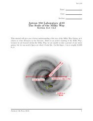
The Ugly...<br />
e<br />
u d<br />
s<br />
µ<br />
c<br />
τ<br />
b<br />
t<br />
10 −4<br />
10 −3<br />
10 −2<br />
ν 1<br />
ν 2<br />
ν 3<br />
m [eV]<br />
10 −1<br />
10 0<br />
10 1<br />
10 2<br />
10 3<br />
10 4<br />
10 5<br />
10 6<br />
10 7<br />
10 8<br />
10 9<br />
10 10<br />
10 11<br />
10 12<br />
Figure 5.6: Order of magnitude of the masses of quarks and leptons.<br />
Order of magnitude of masses of quarks & leptons<br />
ith real positive masses m k .<br />
ritten as<br />
The resulting diagonal mass term can b<br />
−L Mν =<br />
3∑<br />
m k¯ν Rk ν Lk + h.c. =<br />
3∑<br />
m k ν k ν k (5.6.156<br />
Thursday, November 17, 2011<br />
k=1<br />
k=1
The Good...<br />
Already in 1934 Fermi provided an answer<br />
with a theory that prescribed a quantitative relation<br />
between fine structure constant and weak coupling<br />
G F ∼ α/m 2 W<br />
Although Fermi adjusted m W<br />
to accommodate strength and range of nuclear radioactive decays<br />
one can readily obtain a value of m W of<br />
from observed<br />
µ<br />
Answer is off by a factor of 2<br />
40 GeV<br />
decay rate for which proportionality factor is<br />
because discovery of parity violation and neutral currents<br />
was in future and introduces an additional factor 1 − m 2 W /m 2 Z<br />
[ ] [ ]<br />
πα 1<br />
G F = √<br />
2m<br />
2<br />
W<br />
1 − m 2 (1 + ∆r)<br />
W /m2 Z<br />
π/ √ 2<br />
Fermi could certainly not have anticipated<br />
that we now have a renormalizable gauge theory<br />
that allows us to calculate radiative correction<br />
∆r<br />
to his formula<br />
Thursday, November 17, 2011
der el sorted predictions dimensional to rather with operators extreme too highin lengths precision, Weinberg’s by proposing pushing effective Λ to that Lagrangian 10the TeV. factor<br />
ection esorted rder dimensional (2m to rather<br />
Higgs 2 operators extreme<br />
mass<br />
lengths in Weinberg’s by proposing<br />
Radiative effective that Lagrangian the factor<br />
Corrections<br />
rection resorted(2m to rather 2 W + m2<br />
W extreme lengths by proposing that the factor<br />
One of most + Z + m2<br />
m2 Z + H − 4m2<br />
acute m2 H − t ) must vanish; exactly! This<br />
ion. The problem is now “solved” 4m2 t ) must<br />
problems because<br />
vanish;<br />
connected scales<br />
exactly!<br />
as<br />
This<br />
large with asultraviolet divergences<br />
tion. rrection The (2mproblem 2 W<br />
concerns + m2 is<br />
Z<br />
radiative + now m2 “solved”<br />
H − 4m2 t ) must because vanish; scales exactly! as large This as<br />
accommodated by the observations<br />
corrections<br />
once one<br />
to<br />
eliminates<br />
mass appearing<br />
the<br />
in Higgs potential<br />
ition. accommodated The problemby isthe now observations “solved” because once one<br />
V = µ 2 scales eliminates<br />
ΦΦ † as large the<br />
make this stick to all orders and for Λ ≤ 10 TeV, this requires<br />
as<br />
emake accommodated this stick toby allthe orders observations and for Λonce ≤ 10one TeV, eliminates this<br />
+<br />
requires<br />
λ(Φ the † Φ) 2<br />
n make<br />
f, W,<br />
this stick to all orders<br />
self-coupling<br />
and for Λ ≤ 10<br />
radiative<br />
TeV, this requires<br />
and H<br />
corrections to Higgs mass are<br />
H<br />
H<br />
f<br />
f<br />
H<br />
H<br />
i Y f<br />
2<br />
2<br />
∫ Λ<br />
d 4 k<br />
(2π) 4 tr(<br />
i<br />
̸ k − m f<br />
i<br />
̸ k+ ̸ p − m f<br />
) ∼ −Λ 2 tr(I)<br />
Y 2<br />
f<br />
32π 2<br />
H<br />
H<br />
W,Z<br />
W,Z<br />
HH<br />
H<br />
i g2<br />
4<br />
∫ Λ<br />
d 4 k 1<br />
(2π) 4 k 2 − m 2 W<br />
∼ Λ 2 g 2<br />
64π 2<br />
Z<br />
m W → m Z<br />
g 2 → g 2 + g ′ 2<br />
H<br />
H<br />
H<br />
H<br />
H<br />
H<br />
H<br />
H<br />
i6λ<br />
∫ Λ<br />
d 4 k 1<br />
(2π) 4 k 2 − m 2 H<br />
∼ Λ 2 3λ<br />
8π 2<br />
m 2 W = 1 4 g2 v 2 , v = 246 GeV, m 2 Z = 1 4 (g2 + g ′2 )v 2 , m 2 f = 1 2 Y 2<br />
f v 2<br />
Y f<br />
is Yukawa coupling<br />
m 2 H =2λv 2 , g g ′ SU(2) L × U(1) Y<br />
λ is quartic Higgs coupling and Λ is a cutoff<br />
Thursday, November 17, 2011<br />
and are gauge couplings
Difference between bare and renormalized masses is<br />
∆µ 2 =<br />
Veltman Condition<br />
⎛<br />
1<br />
⎝9g 2<br />
64π 2 +3g ′2 + 24 λ − 8 ∑ f<br />
N f Y 2<br />
f<br />
⎞<br />
⎠ Λ 2<br />
≃<br />
3<br />
16π 2 v 2 (2m2 W + m 2 Z + m 2 H − 4m 2 t )Λ 2<br />
SM works amazingly well by fixing<br />
at electroweak scale<br />
generally assumed ☛ this indicates existence of new physics beyond SM<br />
Following Weinberg<br />
Λ<br />
L(m W )=|µ 2 | H † H + 1 4 λ(H† H) 2 + L gauge<br />
SM<br />
+ LYukawa SM + 1 Λ L5 + 1 Λ 2 L6 + . . .<br />
where operators of higher dimension parametrize physics beyond SM<br />
Some have resorted to rather extreme lengths by proposing that<br />
factor multiplying unruly quadratic correction<br />
(2m 2 W + m 2 Z + m 2 H − 4m 2 t )<br />
must vanish exactly!<br />
By most conservative estimates this new physics is within our reach<br />
Thursday, November 17, 2011
New Physics at the TeV Scale?<br />
Avoiding fine tuning requires<br />
E.G. for m H = 115 − 200 GeV,<br />
∆µ 2 ∣ ∣∣∣<br />
∣ µ 2 = δv2<br />
v 2<br />
Λ 2 − 3<br />
to be revealed by CERN LHC<br />
≤ 10 ⇒ Λ = 2 − 3 TeV<br />
we have implicity used<br />
v 2 = −µ 2 /λ<br />
[valid in approximation<br />
disregarding terms beyond<br />
Let's contemplate possibilities<br />
O(H 4 )<br />
in Higgs potential]<br />
⌾<br />
Veltman condition happens to be satisfied<br />
and this would leave particle physics with an ugly fine tuning problem<br />
⌾<br />
⌾<br />
This is very unlikely ☛ LHC must reveal Higgs physics<br />
already observed via radiative correction<br />
or at least discover physics that implements Veltman condition<br />
It must appear at<br />
2 − 3TeV<br />
even though higher scales can be rationalized<br />
when accommodating selected experiments<br />
Thursday, November 17, 2011
SUSY<br />
Supersymmetry predicts that interactions exist<br />
that would change fermions into bosons and vice versa<br />
and that all known fermions (bosons) have SUSY boson (fermion) partner<br />
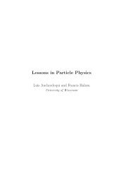
SUSY offers solution of bad behavior of radiative corrections in SM<br />
As for every boson there is a companion fermion<br />
bad divergence associated with Higgs loop<br />
cancelled by a fermion loop with opposite sign<br />
H<br />
Figure 1: Supersymmetry offers a neat solution of the bad behavior of radiative corrections in the<br />
standard model. As for every boson there is a companion fermion, the bad divergence associated<br />
with the Higgs loop is cancelled by a fermion loop with opposite sign.<br />
even though it elegantly controls quadratic divergence<br />
by cancellation of boson and fermion contributions <br />
Let’s contemplate the possibilities. The Veltman condition happens<br />
2 −<br />
to<br />
3TeV<br />
be satisfied and this<br />
would leave particle physics with an ugly fine tuning problem. This is very unlikely; LHC must<br />
reveal the Higgs physics already observed via radiative correction, or at least discover the physics<br />
it is already fine-tuned at a scale of<br />
Thursday, November 17, 2011
The Bad...<br />
Next class<br />
U have a test!<br />
Thursday, November 17, 2011
Thursday, November 17, 2011<br />
Happy thanksgiving