Track A - Water Resources Center - University of Minnesota
Track A - Water Resources Center - University of Minnesota
Track A - Water Resources Center - University of Minnesota

Create successful ePaper yourself
Turn your PDF publications into a flip-book with our unique Google optimized e-Paper software.
Lori A. Krider<br />
Joseph A. Magner<br />
Jim Perry
Investigations<br />
• Temperature regimes <strong>of</strong><br />
groundwater-fed streams<br />
vs. surface water fed<br />
streams<br />
• Affect <strong>of</strong> air temperature<br />
on the water temperature<br />
in groundwater-fed<br />
streams<br />
• Implications for climate<br />
change<br />
• Use in guiding land<br />
management
Importance<br />
• Air temperatures are very influential on surface and<br />
groundwater temperatures (Erickson et al., 2000;<br />
Meisner et al., 1988)<br />
• <strong>Water</strong> temperatures dictate species composition and<br />
cold water habitat supports trout populations<br />
• No published work investigates this relationship in<br />
carbonate systems across watersheds<br />
• Other uses: relate water temperatures to trout growth<br />
patterns and diet; choose study sites when research is<br />
related to water temperature
Study Area<br />
• Southeastern <strong>Minnesota</strong>’s Driftless<br />
Region<br />
• Lacks glacial scouring; old valleys<br />
with dramatic changes in elevation<br />
• Carbonate rocks: made <strong>of</strong> easily<br />
eroded minerals<br />
• Karst geology: well-developed<br />
surface features such as springs and<br />
sinkholes<br />
• Incipient karst geology: seeps and<br />
groundwater recharge through<br />
infiltration
Temperature ( o C)<br />
Time Frame<br />
• “Present” data set<br />
• If climate change<br />
has been escalating<br />
in the past several<br />
decades, how far<br />
back will the<br />
measurements still<br />
represent present<br />
conditions?<br />
9.0<br />
8.5<br />
8.0<br />
7.5<br />
7.0<br />
6.5<br />
6.0<br />
5.5<br />
5.0<br />
Temperature Over Time, 1986 - 2008: Rochester IA<br />
(3-Month Moving Window Average)<br />
1998<br />
1998<br />
Year<br />
Rochester IA: approximately in the middle<br />
<strong>of</strong> our study streams
Data Details<br />
• 7 counties<br />
• 40 study streams<br />
Rice<br />
Goodhue<br />
Wabasha<br />
• 106 temperature<br />
loggers<br />
• 3,606 weekly<br />
averages<br />
Olmstead<br />
Winona<br />
Fillmore<br />
Houston
Data Source<br />
• <strong>Water</strong> temperature data<br />
• STORET, DNR, David Huff and Toby Dogwiler<br />
• Discrete and continuous -> weekly averages<br />
• Year-round, winter intensive or non-winter intensive<br />
• Air temperature data<br />
• NOAA weather stations<br />
• Thiessen polygons were created for six counties<br />
• Between 7.1 km and 53.8 km from the streams they were<br />
matched to
Statistical Analysis<br />
• Linear regression models<br />
(y = mx +b -> T w =B(T a )+A)<br />
• Produces R 2 value (0 – 1)<br />
• How well the model<br />
explains the variation in<br />
the data<br />
• Closer to one is better<br />
• Marginal R 2 improvements<br />
with non-linear models<br />
(between 0.0001 and<br />
0.135)<br />
http://www.unr.edu/math/events/index.html
Terminology<br />
• Regressions explained in terms <strong>of</strong> the project<br />
• Slope: how quickly water temperatures rise as a function<br />
<strong>of</strong> air temperatures<br />
• Intercept: temperature <strong>of</strong> the water when the air<br />
temperature becomes freezing<br />
• R 2 value: how much <strong>of</strong> the variation in stream<br />
temperature can be explained by air temperatures
Temporal Scale<br />
• What is best for regressions <strong>of</strong> groundwater-fed streams?<br />
• Pilgrim et al. (1998): 36 surface water streams and 3<br />
groundwater-fed streams across MN<br />
• monthly produces highest R 2 (Apr. – Oct.)<br />
• Time lags up to 7 days for rivers up to 15 ft deep (Stefan and<br />
Pred’homme, 1993)<br />
• R 2 for a sub-set <strong>of</strong> our streams<br />
• 0.56 at monthly scale, April – October data<br />
• 0.86 at weekly scale, year-round data<br />
• Number <strong>of</strong> data points<br />
• 431 monthly averages, Apr. – Oct.<br />
• 1734 weekly averages, year-round
Results Summary & Comparison<br />
• Slopes, intercepts and R 2 varied much between streams<br />
• Slopes and intercepts were markedly different from<br />
values displayed by surface water fed streams<br />
Study Streams<br />
Slopes<br />
0.18 - 0.74<br />
Intercepts<br />
2.90 - 8.29<br />
Pilgrim et al.’s Study Streams<br />
Slopes<br />
0.85 - 1.15<br />
Intercepts<br />
-1.51 - 4.01
Average Weekly <strong>Water</strong> Temperature (C)<br />
Average Weekly <strong>Water</strong> Temperature (C)<br />
Exemplary Results<br />
20.00<br />
Snake Creek Weekly Linear Regression<br />
1999 - 2000, 2003, 2005, 2007<br />
y = 0.3218x + 7.3901<br />
R² = 0.591<br />
Winnebago Creek Weekly Linear Regression<br />
2000 - 2003 & 2008<br />
20<br />
y = 0.3424x + 6.93<br />
R² = 0.9771<br />
15.00<br />
15<br />
10.00<br />
10<br />
5.00<br />
5<br />
0.00<br />
0.00 5.00 10.00 15.00 20.00 25.00 30.00<br />
Average Weekly Air Temperature (C)<br />
0<br />
-20 -15 -10 -5 0 5 10 15 20 25 30<br />
Average Weekly Air Temperature (C)<br />
Lowest R 2<br />
Highest R 2
Average Weekly <strong>Water</strong> Temperature (C)<br />
Lumped Model<br />
Our Study Streams<br />
Slope: 0.38<br />
Intercept: 6.63<br />
R 2 value: 0.83<br />
SE: 1.98<br />
SD: 4.79<br />
Pilgrim et al.’s Study Streams<br />
Slope: 0.97<br />
Intercept: 1.88<br />
All Streams Weekly Regression<br />
1999 - 2008<br />
25<br />
20<br />
15<br />
10<br />
5<br />
y = 0.3819x + 6.6257<br />
R² = 0.82913<br />
0<br />
-30 -20 -10 0 10 20 30<br />
Average Weekly Air Temperature (C)
Intercept<br />
Mechanisms <strong>of</strong> Control<br />
• Adapted from<br />
O’Driscoll and<br />
DeWalle (2004)<br />
• Our R 2 is<br />
considerably<br />
lower (vs. 0.89)<br />
• due to spatial<br />
and temporal<br />
differences<br />
• Protection vs.<br />
restoration<br />
9<br />
8<br />
7<br />
6<br />
5<br />
4<br />
3<br />
Slope vs. Intercept<br />
All Streams Weekly Linear Regression<br />
Groundwater Control<br />
BSC<br />
NBC<br />
Gil C<br />
CSB<br />
Co C<br />
Ba C<br />
He C<br />
Be C<br />
y = -4.6744x + 8.1617<br />
R² = 0.3893<br />
0 0.1 0.2 0.3 0.4 0.5 0.6 0.7 0.8 0.9<br />
Slope<br />
Ma BW<br />
Ru C<br />
No BW<br />
SD = 0.13, SE = 0.10<br />
Pi C<br />
Meteorological Control<br />
NFZR
Contributing Factors<br />
• Factors that affect the air-water temperature relationship<br />
• No/little effect on R 2 , slope or intercept<br />
• Number <strong>of</strong> weekly averages (< .0.08 for all)<br />
• Number <strong>of</strong> known springs within 50 m (< 0.07 for all)<br />
• Number <strong>of</strong> known springs within 250 m (< 0.005 for all)<br />
• Number <strong>of</strong> temperature loggers (< 0.11 for all)<br />
• Minor watershed area (acres) (< 0.14 for both R 2 & intercept)<br />
• Some effect on R 2 , slope or intercept<br />
• Minor watershed area vs. slope (R 2 = 0.36)
Groundwater vs. Surface <strong>Water</strong><br />
• Groundwater-fed streams have drastically different<br />
temperature regimes than surface water fed streams<br />
• Comparison between slopes and intercepts<br />
• Groundwater input doesn’t affect the strength <strong>of</strong> the airwater<br />
temperature correlation<br />
Our Study Streams<br />
R 2 values: range<br />
0.59 - 0.98<br />
R 2 values: lumped<br />
0.83<br />
Pilgrim et al. Study Streams<br />
R 2 values: range<br />
0.67 - 0.96<br />
R 2 values: lumped<br />
0.83
Other Findings<br />
• Could not provide concrete evidence that the amount <strong>of</strong><br />
groundwater input affects R 2 , slope, or intercept<br />
• Incomplete karst inventory database<br />
• Groundwater inputs are difficult to quantify accurately<br />
• Graphing slope vs. intercept suggests mechanisms for<br />
control<br />
• Asymptote near or above 0 o C water temperatures with<br />
air temperatures well below 0 o C<br />
• Surface water fed streams asymptote at 0 o C water<br />
temperatures with air temperatures at 0 o C
Groundwater Inflow<br />
• Most important<br />
determinant <strong>of</strong> water<br />
temperatures in<br />
groundwater-fed streams<br />
• Discharge<br />
• Lentz farm<br />
• Stream velocity<br />
• Shade<br />
• Source <strong>of</strong> resurgence<br />
• <strong>Water</strong> table vs. interflow<br />
Artisan spring on Ralph Lentz farm:<br />
400 gallons /minute
Implications for Climate Change<br />
• Streams in northerly climates do not always follow unity<br />
at air temperatures > 20 o C<br />
• Suggested by Mohensi & Stefan, 2000<br />
• Varies from stream to stream: some level slightly, some<br />
follow unity and some produce more scatter<br />
• Streams that follow unity and have high R 2 values are<br />
most promising as predictive tools<br />
• Streams with higher slopes and lower intercepts are<br />
more susceptible
Climate Change Continued<br />
• A1B SRES regional climate change scenario for central<br />
North America<br />
• 2.4 and 6.4 o C above 2000 conditions for the summer<br />
months (June – August) by the years 2080 – 2099 (IPCC<br />
Working Group I, 2007)<br />
• Transform marginal or near marginal habitat into unsuitable<br />
habitat<br />
• Restrict suitable summer habitat to directly downstream <strong>of</strong><br />
springs and expand suitable winter habitat (Meisner et al.,<br />
1988)
Management for Mitigation<br />
•Increase snow trapping in riparian areas<br />
•Provide riparian shading<br />
•Encourage stream deepening and<br />
narrowing<br />
•Reduce temperatures <strong>of</strong> shallow<br />
groundwater aquifer
Literature Cited<br />
• Brooks, K. N., P. F. Ffolliott, H. M. Gregersen, & L. F. DeBano. 2003. Hydrology and the Management <strong>of</strong><br />
<strong>Water</strong>sheds (3 rd ed.). Ames, Iowa: Iowa State <strong>University</strong> Press.<br />
• Coldwater Fish and Fisheries Working Group. 2010. Wisconsin Initiative on Climate Change Impacts. First<br />
Report: Released February 2011.<br />
• Cristea, N., & J. Janisch. 2007. Modeling the Effects <strong>of</strong> Riparian Buffer Width and Effective Shade and<br />
Stream Temperature. Environmental Assessment Program <strong>of</strong> the Washington State Department <strong>of</strong><br />
Ecology. Publication No. 07-03-028.<br />
• Erickson, T. R. & H. Stefan. 2000. Linear Air/<strong>Water</strong> Temperature Correlations for Streams During Open<br />
<strong>Water</strong> Periods. Journal <strong>of</strong> Hydrological Engineering 5(3): 317 – 321.<br />
• Intergovernmental Panel on Climate Change Working Group I. 2007. Contribution <strong>of</strong> the Working Group I<br />
to the Fourth Assessment Report <strong>of</strong> the Intergovernmental Panel on Climate Change, 2007. Accessed<br />
online 10 April 2011.<br />
• Meisner, J. D., Rosenfeld, J. S., & Regier. 1988. The Role <strong>of</strong> Groundwater in the Impact <strong>of</strong> Climate Warming<br />
on Stream Salmonines. Fisheries 13(3): 2 -8.<br />
• Mohensi, O., H. G. Stefan & T. R. Erickson. 1998. A nonlinear regression model for weekly stream<br />
temperatures. <strong>Water</strong> <strong>Resources</strong> Research 34: 2685 – 2692.<br />
• O’Driscoll, M. A., & DeWalle, D. R. 2004. Stream-Air Temperature Relationships as Indicators <strong>of</strong><br />
Groundwater Inputs. AWRA <strong>Water</strong>shed Update 2(6).<br />
• Pilgrim, J., X. Fang & H. Stefan. 1998. Stream Temperature Correlations with Air Temperatures in<br />
<strong>Minnesota</strong>: Implications for Climate Warming. Journal <strong>of</strong> the American <strong>Water</strong> <strong>Resources</strong> Association<br />
34(5): 1109 – 1121.<br />
• Stefan, H. G. & E. B. Preud’homme. 1993. Stream Temperature Estimation from Air Temperature. <strong>Water</strong><br />
<strong>Resources</strong> Bulletin 29(1): 27 – 46.
Natural short-term declines in curly-leaf pondweed across a<br />
network <strong>of</strong> sentinel lakes: potential impacts <strong>of</strong> snowy winters<br />
Ray Valley, Steve Heiskary, Cindy Tomcko
Comprehensive report is in the<br />
works<br />
• Covers findings here<br />
in addition:<br />
• Correlations between<br />
water quality and<br />
curly-leaf growth and<br />
summer plant growth<br />
• Case studies<br />
• Suggested future<br />
investigations
Sustaining Lakes in a Changing Environment<br />
(SLICE)<br />
‣ 24 sentinel lakes; sites <strong>of</strong> cooperative<br />
long-term monitoring and research.<br />
DNR, PCA, USGS, SNF major<br />
partners<br />
‣ <strong>Water</strong> quality, zooplankton, aquatic<br />
plants, fish and continuous<br />
temperature data monitored since<br />
2008<br />
‣ Curly-leaf pondweed (CLP) occurs in<br />
14; annual spring surveys (pointintercept)<br />
in 11
Assessment Methods – Point Intercept<br />
• Conducted during the<br />
peak <strong>of</strong> growth (typically<br />
late May/Early June)<br />
• Rake throws at uniformly<br />
space points spaced 80-m<br />
apart.<br />
• % Frequency is correlated<br />
with % areal cover
Genesis: Serendipity<br />
• Noticed declines in CLP cover across<br />
most sentinel lakes since monitoring<br />
began in 2008.<br />
• Due to simultaneous declines across<br />
network, knew immediately that something<br />
environmental must be going on.
Curly-leaf declines<br />
37%<br />
decline<br />
overall<br />
80%<br />
95%
Decline in surface growth in Pearl<br />
Lake (Stearns Co.)<br />
22.6% 0.75% 0.5%
Hmm…
Curly-leaf pondweed life history<br />
‣ Invasive plant that’s<br />
been present in MN<br />
since 1907.<br />
‣ Can grow abundantly<br />
in spring then<br />
senesces in July<br />
‣ Algae blooms <strong>of</strong>ten<br />
follow senescence in<br />
productive lakes
Curly-leaf distribution<br />
‣ Documented in 730 lakes;<br />
probably occurs in many<br />
more<br />
‣ Most are found in the<br />
central transition forest<br />
landtype (min <strong>of</strong> 5% <strong>of</strong> all<br />
lakes w/ DNR ID#’s).<br />
‣ Speculation that range is<br />
expanding northward
Curly-leaf pondweed life history<br />
‣ Produces turion<br />
propagules in summer.<br />
‣ Turion production is<br />
correlated with<br />
temperature and<br />
photoperiod<br />
‣ Turions sprout in fall<br />
and plant overwinters<br />
green<br />
‣ Boom-bust growth in<br />
south, not so in the<br />
north<br />
‣ Good info on life<br />
history; not on<br />
ecosystem effects
Conservation value in the South<br />
‣ In many SW prairie lakes<br />
and urban lakes, CLP is<br />
one <strong>of</strong> only a few plant<br />
spp. that grow<br />
‣ Supports vegetation<br />
dependent native fish<br />
communities in the SW<br />
(e.g., largemouth bass,<br />
bluegill, northern pike)<br />
‣ Killing the plant in these<br />
lakes may do more harm<br />
than good in terms <strong>of</strong><br />
habitat and WQ if no<br />
natives come in behind.
Back to the question – Curlyleaf<br />
declines – what might be<br />
going on here?
37%<br />
decline<br />
overall<br />
Curly-leaf declines
Growing Season<br />
Differences?
Growing<br />
Degree<br />
Days<br />
Departure<br />
from<br />
Normal
Nah that’s not it –<br />
2010 was actually<br />
very warm and CLP<br />
growth was lowest<br />
we’ve seen
Links to spring water<br />
temperatures?<br />
In other words, cooler<br />
springs = less growth?
Nah that’s not it –<br />
spring water temps<br />
have gotten warmer<br />
since 2008
Spring <strong>Water</strong> Temperatures (°C<br />
Ice-<strong>of</strong>f - May 31st)<br />
16<br />
14<br />
12<br />
10<br />
8<br />
6<br />
2008<br />
2009<br />
2010<br />
4<br />
2<br />
0<br />
St. Olaf Pearl St. James Portage Peltier
Links to ice cover<br />
duration?<br />
In other words,<br />
increases in ice-cover<br />
duration = reduced<br />
growth?
Nope not it either –<br />
duration <strong>of</strong> ice cover<br />
has gotten shorter<br />
since 2008 (34 fewer<br />
days in St. James<br />
between 2008 and<br />
2010)
Days <strong>of</strong> Ice<br />
180<br />
160<br />
140<br />
120<br />
100<br />
80<br />
60<br />
2008<br />
2009<br />
2010<br />
40<br />
20<br />
0<br />
St. Olaf Pearl St. James Portage Peltier
Links to snow cover?<br />
In other words,<br />
increases in snow cover<br />
early in winter =<br />
reduced growth?
EUREKA!!
Dec. + Jan. Snowfall (in) Departure from 1971-2000<br />
Normal<br />
40<br />
St. Olaf Pearl St. James Portage Peltier<br />
30<br />
20<br />
10<br />
0<br />
-10<br />
-20<br />
-30<br />
2000 2002 2004 2006 2008 2010 2012<br />
Year
Findings<br />
• Winters during most <strong>of</strong> the 2000’s were<br />
less snowy than normal<br />
• Easy winters for CLP expansion<br />
• Last few winters have been snowier than<br />
normal.<br />
• Stressful on overwintering CLP plants<br />
needing light for basal metabolism
What did 2011 bring?
Dec. + Jan. Snowfall (in) Departure from<br />
1971-2000 Normal<br />
Winter was even snowier<br />
40<br />
30<br />
20<br />
10<br />
0<br />
-10<br />
-20<br />
-30<br />
2000 2002 2004 2006 2008 2010 2012<br />
Year<br />
St. Olaf Pearl St. James Portage Peltier
Curly-leaf declines leveled <strong>of</strong>f
Implications <strong>of</strong> Climate Change<br />
• Winters and ice-cover will be shorter<br />
(Fang and Stefan 2000, 2009)<br />
• Regional variability on effects on the<br />
underwater environment:<br />
• Dependent on water levels, eutrophication,<br />
and winter snowfall (Danylchuk and Tonn<br />
2003)
Winters may get snowier in the<br />
north; rainier in the South
Critical Temp Thresholds<br />
High turion production; rapid senescence<br />
Turions start to form
Temperature Mediation <strong>of</strong> CLP<br />
‣ Some northern lakes never get warm<br />
enough to facilitate high turion production<br />
and rapid senescence.<br />
‣ CLP exists in northern lakes but rarely at<br />
high levels and usually all-yr round.<br />
‣ As climate change increases summer<br />
temperatures, so too can conditions<br />
conducive to abundant CLP growth
Summary<br />
• Winter possibly plays some role in limiting curly-leaf<br />
pondweed growth<br />
• Results from 2011 neither refute nor confirm a<br />
relationship. Follow up studies are needed.<br />
• Future CLP status in the north may depend on<br />
interplay <strong>of</strong> changes in snowfall and summer water<br />
temperatures
Suggested Future Investigations<br />
• A more comprehensive analysis <strong>of</strong> the response <strong>of</strong><br />
biota to curly-leaf proliferation.<br />
• Controlled studies in well-defined sites (e.g.<br />
mesocosm studies) could allow for improved<br />
understanding <strong>of</strong> curly-leaf response to snow cover<br />
• The correlation <strong>of</strong> curly-leaf cover to water quality<br />
varies among lakes. The sentinel lakes may provide<br />
a good opportunity to better quantify and model the<br />
impact <strong>of</strong> curly-leaf senescence on lake water<br />
quality – take advantage <strong>of</strong> our free data!!
Acknowledgments<br />
• DNR Area Fisheries & Fisheries Research Unit<br />
• Master Naturalist Program<br />
• MPCA <strong>Water</strong> Monitoring Unit<br />
• MN Climate Working Group<br />
Funding – DNR Game and Fish Fund, Environment and<br />
Natural Resource Trust Fund, Sportfish Restoration,<br />
MPCA, Volunteers
EARLY-WINTER<br />
INVERTEBRATE POPULATIONS<br />
IN TROUT STREAMS<br />
OF SOUTHEASTERN MN<br />
Jane Louwsma Mazack, <strong>University</strong> <strong>of</strong> <strong>Minnesota</strong>
Acknowledgements<br />
Will French<br />
Jennifer Biederman<br />
Pat Sherman<br />
Lori Krider<br />
Bruce Vondracek<br />
Jim Perry<br />
Len Ferrington<br />
Petra Kranzfelder<br />
Jessica Miller
Introduction<br />
Groundwater-fed streams in southeastern <strong>Minnesota</strong><br />
are recreationally and economically valuable
Introduction<br />
Trout streams in SE MN are thermally buffered by<br />
groundwater input<br />
Cooler summer temperatures<br />
Warmer winter temperatures<br />
Gribben Creek
Introduction<br />
Cold-adapted (stenotherm) insects are <strong>of</strong>ten<br />
abundant in these streams<br />
Diamesa grow at stream temperatures from 2-10 o C<br />
Stenotherm genera include:<br />
Diamesa<br />
Prodiamesa<br />
Micropsectra<br />
Brachycentrus<br />
Adult Diamesa (Chironomidae)
A Conceptual Model<br />
Climate ?<br />
Geomorphology<br />
Riparian zone<br />
Land use<br />
Thermal<br />
buffering<br />
capacity<br />
Aquatic<br />
Invertebrate<br />
community<br />
Trout growth<br />
& abundance
Research Questions<br />
1. What is the diversity, composition, and<br />
heterogeneity <strong>of</strong> winter invertebrate communities<br />
in groundwater-fed trout streams?<br />
2. What is the relationship between stream thermal<br />
regime and invertebrate community<br />
characteristics?<br />
3. What is the relationship between invertebrate<br />
communities and winter trout diet and condition?
Sampling Sites<br />
12 stream reaches in southeastern <strong>Minnesota</strong>
Sampling Methods<br />
Early, mid, and late winter samples<br />
Paired with brown trout diets<br />
In each sample event:<br />
5 Hess samples<br />
10 minute dipnet sample<br />
10 minutes pupal exuviae collection
Sample Analyses<br />
Simpson’s Index with jack-knifing<br />
Measure <strong>of</strong> population diversity (D)<br />
Range from 0 < D < 1<br />
• 0 represents no diversity<br />
• 1 represents infinite diversity<br />
Whittaker’s Percentage Similarity<br />
Measure <strong>of</strong> within-reach heterogeneity<br />
Range from 0 to 1<br />
• 0 represents complete heterogeneity<br />
• 1 represents complete homogeneity
Question 1<br />
1. What is the diversity, composition, and<br />
heterogeneity <strong>of</strong> winter invertebrate communities<br />
in groundwater-fed trout streams?
Number <strong>of</strong> Genera Present<br />
Community Characteristics<br />
70<br />
60<br />
50<br />
40<br />
30<br />
20<br />
73.6<br />
individuals/<br />
meter 2<br />
761<br />
individuals/<br />
meter 2<br />
10<br />
0<br />
Sample Site
Diversity (Simpson's Index)<br />
Community Characteristics<br />
1<br />
R² = 0.8012<br />
0.9<br />
0.8<br />
0.7<br />
0.6<br />
0.5<br />
0.4<br />
0.3<br />
0.2<br />
0.1<br />
0<br />
0 5 10 15 20 25 30 35<br />
Number <strong>of</strong> Genera Present
Diversity (Simpson's Index)<br />
Community Characteristics<br />
1<br />
0.9<br />
0.8<br />
0.7<br />
0.6<br />
0.5<br />
0.4<br />
0.3<br />
0.2<br />
0.1<br />
0<br />
Sample Site
Diversity (Simpson's Index)<br />
Community Characteristics<br />
1<br />
0.9<br />
0.8<br />
0.7<br />
0.6<br />
0.5<br />
0.4<br />
0.3<br />
0.2<br />
0.1<br />
0<br />
Sample Site
Community Characteristics<br />
North Branch<br />
Trout Run<br />
4% 2% EPT<br />
4% 2%<br />
11%<br />
19%<br />
23%<br />
EPT<br />
Stenotherms<br />
30%<br />
71%<br />
Diptera<br />
Other<br />
8%<br />
51%<br />
94%<br />
51%
Whittaker's Similarity<br />
Community Characteristics<br />
1.2<br />
1<br />
0.8<br />
0.6<br />
0.4<br />
0.2<br />
0<br />
Sample Site
Question 2<br />
1. What is the relationship between stream thermal<br />
regime and invertebrate community<br />
characteristics?<br />
Adult Diamesa (Chironomidae)
Slope <strong>of</strong> water-air temperature regression<br />
Stream Thermal Regime<br />
0.6<br />
0.5<br />
0.4<br />
0.3<br />
0.2<br />
y = -0.0004x + 0.5306<br />
R² = 0.5924<br />
0.1<br />
0<br />
0 100 200 300 400 500 600 700 800<br />
Density (Individuals/m 2 )
Question 3<br />
1. What is the relationship between invertebrate<br />
communities and winter trout diet and condition?
Delta Wr<br />
Trout Condition<br />
Mean Delta Wr<br />
15<br />
10<br />
5<br />
A<br />
AB<br />
A<br />
F=11.78<br />
P
Delta Wr<br />
Diversity (Simoson's Index)<br />
Trout Condition<br />
1<br />
15<br />
10<br />
5<br />
A<br />
Mean Delta Wr<br />
AB<br />
A<br />
F=11.78<br />
P
Conclusion<br />
1. Early-winter trout stream invertebrate communities<br />
exhibit a wide range <strong>of</strong> diversity, heterogeneity,<br />
and density.<br />
2. Streams with lower temperature variability tend to<br />
have larger early-winter invertebrate communities.<br />
3. In preliminary analysis, the least diverse<br />
invertebrate community reflected the highest rate<br />
<strong>of</strong> overwinter brown trout growth.
Conclusion<br />
Climate ?<br />
Geomorphology<br />
Riparian zone<br />
Land use<br />
Thermal<br />
buffering<br />
capacity<br />
Aquatic<br />
Invertebrate<br />
community<br />
Trout growth<br />
& abundance