WONDERFUL UNIVERSE - American Museum of Natural History
WONDERFUL UNIVERSE - American Museum of Natural History
WONDERFUL UNIVERSE - American Museum of Natural History

Create successful ePaper yourself
Turn your PDF publications into a flip-book with our unique Google optimized e-Paper software.
Science Research Mentoring Program<br />
<strong>WONDERFUL</strong><br />
<strong>UNIVERSE</strong><br />
This course addresses core concepts in astrophysics: energy and force,<br />
conservation laws, Newton’s laws, gravity and orbits, quantization, light, and<br />
space-time. Light topics include spectroscopy and electron energy levels, photos<br />
versus waves, the electromagnetic spectrum, and blackbody radiation. The<br />
course also covers basic mathematical skills, including units <strong>of</strong> measurement,<br />
scientific notation, and trigonometry. Activities and planetarium viewings<br />
reinforce each topic.<br />
Organization:<br />
• Each activity and demonstration is explained under its own heading.<br />
• If an activity has a handout, you will find that handout on a separate page .<br />
• If an activity has a worksheet that students are expected to fill out, you will<br />
find that worksheet on a separate page.<br />
• Some additional resources (program and script) are included as separate<br />
files.<br />
2<br />
13<br />
16<br />
20<br />
24<br />
28<br />
30<br />
37<br />
42<br />
51<br />
57<br />
62<br />
Session 1: The Universe: How Big Is It And How Much Is In It?<br />
Session 2: Unit and Math Primer<br />
Session 3: Conservation Is The Name Of The Game<br />
Session 4: Forces and Acceleration, Newton and Motion<br />
Session 5: Orbits, Kepler, Gravity, Conic Sections<br />
Session 6: Light — Basics <strong>of</strong> Optics (Ray Optics)<br />
Session 7: Wave Optics<br />
Session 8: Electromagnetic Spectrum<br />
Session 9: Electromagnetic Processes<br />
Session 10: Light And The Atom<br />
Session 11: Special Relativity<br />
Session 12: General Relativity<br />
The Science Research Mentoring Program is supported by NASA under grant award NNX09AL36G.<br />
1
Science Research Mentoring Program<br />
<strong>WONDERFUL</strong> <strong>UNIVERSE</strong><br />
Session One: The Universe: How Big Is It And How<br />
Much Is In It?<br />
learning objectives<br />
Students will understand size and distance scaling. Students will gain a sense <strong>of</strong> sizes and<br />
variety <strong>of</strong> objects in the universe, and the size <strong>of</strong> the universe itself.<br />
key topics<br />
• Distance units<br />
• SI units and prefixes<br />
• Estimation<br />
Class outline<br />
time<br />
35 minutes<br />
15 minutes<br />
15 minutes<br />
15 minutes<br />
20 minutes<br />
15 minutes<br />
5 minutes<br />
TOPIC<br />
Registration / Pre-<br />
Assessment<br />
Course Introduction<br />
ACTIVITY: Sorting<br />
Objects<br />
Defining Astronomy<br />
DEMONSTRATION:<br />
Grand Tour <strong>of</strong> the<br />
Universe<br />
ACTIVITY: Objects in the<br />
Universe<br />
Wrap Up<br />
description<br />
Check-in for students, including all paperwork, plus a preassessment<br />
testing knowledge about topics covered in this<br />
course (post-assessment for the last class should be identical).<br />
Introduce instructors, course topics and expectations, brief<br />
icebreaker for students.<br />
Students consider sizes <strong>of</strong> various objects in the universe versus<br />
distances to/between them.<br />
Define terms: “astronomy,” “astrophysics,” and “universe.”<br />
Introduce astronomical units, light years and parsecs, showing<br />
a meter stick for reference (optional). Note exponential versus<br />
scientific notation, and SI prefixes.<br />
Use a digital system to take a Grand Tour <strong>of</strong> the observable<br />
universe. Note types <strong>of</strong> objects and distances between them, as<br />
well as the structure <strong>of</strong> the universe.<br />
Investigate some <strong>of</strong> the objects in the universe more closely.<br />
Review material from the day.<br />
MATERIALS<br />
Pre-assessment (not provided), Sorting Objects packets,<br />
meter stick (optional), laser pointer (optional)<br />
PREP WORK<br />
Make copies <strong>of</strong> Sorting Object packets, including one <strong>of</strong><br />
each images included below.<br />
A/V NeedeD<br />
Lights and projections for planetarium, or similar<br />
HOMEWORK<br />
None<br />
Halls used<br />
Hayden Planetarium, Cullman Hall <strong>of</strong> the Universe, Scales<br />
<strong>of</strong> the Universe (optional)<br />
© 2013 <strong>American</strong> <strong>Museum</strong> <strong>of</strong> <strong>Natural</strong> <strong>History</strong>. All Rights Reserved. 2
Science Research Mentoring Program<br />
<strong>WONDERFUL</strong> <strong>UNIVERSE</strong><br />
Session One: The Universe: How Big Is It And How Much Is In It?<br />
ACTIVITY: Sorting Objects<br />
Have copies <strong>of</strong> the objects sorted into packets that<br />
have one <strong>of</strong> each image provided below. Divide<br />
students into groups <strong>of</strong> NN and hand out one packet<br />
to each group. Explain that in astronomy we think a<br />
lot about how large and far away things are. In this<br />
context, “large” refers to volume, not mass.<br />
Ask the students to order the objects by size<br />
(diameter) and distance from us (how far away, at<br />
closest approach). They should discuss and record<br />
both lists, then review them as a class.<br />
DEMONSTRATION: Grand Tour <strong>of</strong> the Universe<br />
This is ideally shown in a planetarium using a digital projection system with s<strong>of</strong>tware such as<br />
Uniview, you can use a classroom projector hooked up to a computer with similar s<strong>of</strong>tware. The<br />
s<strong>of</strong>tware should be able to show the 3-dimensional positions <strong>of</strong> objects, allowing you to move<br />
towards and around objects. (This is different from s<strong>of</strong>tware like Google Sky, with which you can<br />
only zoom in on objects.) Suggested platforms include the <strong>American</strong> <strong>Museum</strong> <strong>of</strong> <strong>Natural</strong> <strong>History</strong>’s<br />
Digital Universe Atlas running within s<strong>of</strong>tware called Partiview (available for free at http://www.<br />
haydenplanetarium.org/universe), Celestia (available for free at http://www.shatters.net/celestia/),<br />
or World Wide Telescope, but other free and commercial s<strong>of</strong>tware exists as well.<br />
For the tour, move out from Earth, showing objects <strong>of</strong> various sizes and distance for reference<br />
along the way. These might include: International Space Station, moon, near Earth asteroids,<br />
planets, exoplanets, nearby stars, farthest radio signals, open or globular clusters, Large and Small<br />
Magallanic Clouds, Andromeda Galaxy, Virgo Cluster, Great Wall and large scale structure <strong>of</strong><br />
universe, quasars, Cosmic Microwave Background image from WMAP or Plank.<br />
© 2013 <strong>American</strong> <strong>Museum</strong> <strong>of</strong> <strong>Natural</strong> <strong>History</strong>. All Rights Reserved. 3
Science Research Mentoring Program<br />
<strong>WONDERFUL</strong> <strong>UNIVERSE</strong><br />
Session One: The Universe: How Big Is It And How Much Is In It?<br />
ACTIVITY: Objects in the Universe<br />
In groups, students explore a section <strong>of</strong> the Hall <strong>of</strong> the Universe and list types <strong>of</strong> objects in the<br />
universe, including those they remember from the Grand Tour.<br />
Come together and list all objects, noting scale models for reference. (In the Cullman Hall <strong>of</strong> the<br />
Universe, view the Scales <strong>of</strong> the Universe models <strong>of</strong> local group, sun, stars, planets.) End next to the<br />
Universe Wall, and discuss percent <strong>of</strong> elements, and <strong>of</strong> “normal” matter, dark matter and dark energy<br />
in the universe.<br />
If Hall <strong>of</strong> the Universe is not available, students can work in groups to brainstorm types <strong>of</strong><br />
astronomical objects. Groups share their lists with the class, and discuss sizes <strong>of</strong> various objects.<br />
Or prepare a power point presentation <strong>of</strong> various astronomical objects (different types <strong>of</strong> stars,<br />
star cluster, nebulae, and galaxies; quasars) and have students describe and discuss. Explain that<br />
“normal” matter makes up a small percentage <strong>of</strong> the universe. Note percentages <strong>of</strong> hydrogen,<br />
helium, compared to other elements, and percentages and <strong>of</strong> dark matter and dark energy in the<br />
universe.<br />
© 2013 <strong>American</strong> <strong>Museum</strong> <strong>of</strong> <strong>Natural</strong> <strong>History</strong>. All Rights Reserved. 4
Science Research Mentoring Program<br />
<strong>WONDERFUL</strong> <strong>UNIVERSE</strong><br />
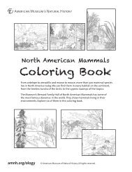
ACTIVITY: Objects in the Universe<br />
The<br />
Moon<br />
© 2013 <strong>American</strong> <strong>Museum</strong> <strong>of</strong> <strong>Natural</strong> <strong>History</strong>. All Rights Reserved. 5
Science Research Mentoring Program<br />
<strong>WONDERFUL</strong> <strong>UNIVERSE</strong><br />
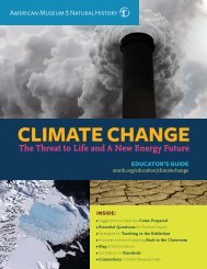
ACTIVITY: Objects in the Universe<br />
The<br />
Orion<br />
Nebula<br />
© 2013 <strong>American</strong> <strong>Museum</strong> <strong>of</strong> <strong>Natural</strong> <strong>History</strong>. All Rights Reserved. 6
Science Research Mentoring Program<br />
<strong>WONDERFUL</strong> <strong>UNIVERSE</strong><br />
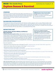
ACTIVITY: Objects in the Universe<br />
Andromeda Galaxy<br />
© 2013 <strong>American</strong> <strong>Museum</strong> <strong>of</strong> <strong>Natural</strong> <strong>History</strong>. All Rights Reserved. 7
Science Research Mentoring Program<br />
<strong>WONDERFUL</strong> <strong>UNIVERSE</strong><br />
ACTIVITY: Objects in the Universe<br />
International Space Station<br />
© 2013 <strong>American</strong> <strong>Museum</strong> <strong>of</strong> <strong>Natural</strong> <strong>History</strong>. All Rights Reserved. 8
Science Research Mentoring Program<br />
<strong>WONDERFUL</strong> <strong>UNIVERSE</strong><br />
ACTIVITY: Objects in the Universe<br />
Eiffel Tower<br />
© 2013 <strong>American</strong> <strong>Museum</strong> <strong>of</strong> <strong>Natural</strong> <strong>History</strong>. All Rights Reserved. 9
Science Research Mentoring Program<br />
<strong>WONDERFUL</strong> <strong>UNIVERSE</strong><br />
ACTIVITY: Objects in the Universe<br />
Saturn<br />
© 2013 <strong>American</strong> <strong>Museum</strong> <strong>of</strong> <strong>Natural</strong> <strong>History</strong>. All Rights Reserved. 10
Science Research Mentoring Program<br />
<strong>WONDERFUL</strong> <strong>UNIVERSE</strong><br />
ACTIVITY: Objects in the Universe<br />
Stephen’s Quintet<br />
© 2013 <strong>American</strong> <strong>Museum</strong> <strong>of</strong> <strong>Natural</strong> <strong>History</strong>. All Rights Reserved. 11
Science Research Mentoring Program<br />
<strong>WONDERFUL</strong> <strong>UNIVERSE</strong><br />
ACTIVITY: Objects in the Universe<br />
The<br />
Sun<br />
© 2013 <strong>American</strong> <strong>Museum</strong> <strong>of</strong> <strong>Natural</strong> <strong>History</strong>. All Rights Reserved. 12
Science Research Mentoring Program<br />
<strong>WONDERFUL</strong> <strong>UNIVERSE</strong><br />
Session Two: Unit and Math Primer<br />
learning objectives<br />
Students will be able to distinguish between base quantities and derived quantities, and know<br />
basic units for length, time, and mass. Students will understand how to use trigonometric<br />
functions to determine distances <strong>of</strong> objects.<br />
key topics<br />
• Base quantities<br />
• Units<br />
• Parallax<br />
Class outline<br />
time<br />
10 minutes<br />
10 minutes<br />
20 minutes<br />
45 minutes<br />
30 minutes<br />
5 minutes<br />
TOPIC<br />
Review<br />
Estimation<br />
Units and Angles Review<br />
ACTIVITY: Measuring<br />
with Parallax<br />
Parallax<br />
Wrap Up<br />
description<br />
Review from last class, listing and discussing objects in the<br />
universe.<br />
Discuss estimation and show an example. For example, estimate<br />
the mass in the universe by multiplying the mass <strong>of</strong> stars, stars<br />
per galaxy, and galaxies in the universe.<br />
Define base quantities and their units. Define derived quantities<br />
and introduce unit analysis. Review angle measurements with<br />
students, including degrees, arcminutes, and arcseconds.<br />
Measurement <strong>of</strong> anglesangles and basic trigonometric functions<br />
(SOHCAHTOA).<br />
Measure angles and use trigonometric functions to determine<br />
unknown distance and height <strong>of</strong> an object.<br />
Define parallax. Discuss how it is used to measure distances<br />
(Gaia is example). Relate to measurement and calculations from<br />
Measuring with Parallax Activity.<br />
Summarize material from the day. Hand out article and problem<br />
set 1.<br />
MATERIALS<br />
Measuring tapes (long and short), masking tape, plumb<br />
bob (or similar), calculators, large demo protractor,<br />
sextants, white board & markers<br />
PREP WORK<br />
Make sextants ahead <strong>of</strong> time, if necessary; tape meter<br />
sticks around classroom for eye-height measurement;<br />
measure height <strong>of</strong> a tall object; make copies <strong>of</strong> article and<br />
problem set 1, make copies <strong>of</strong> worksheet.<br />
A/V NeedeD<br />
None<br />
HOMEWORK<br />
Reading for discussion in next class (recommend recent<br />
article about Gaia); problem set with practical problems<br />
involving parallax, estimation, and scales <strong>of</strong> objects<br />
Halls used<br />
Large space, such as the Cullman Hall <strong>of</strong> the Universe<br />
© 2013 <strong>American</strong> <strong>Museum</strong> <strong>of</strong> <strong>Natural</strong> <strong>History</strong>. All Rights Reserved. 13
Science Research Mentoring Program<br />
<strong>WONDERFUL</strong> <strong>UNIVERSE</strong><br />
Session Two: Unit and Math Primer<br />
ACTIVITY: Measuring with Parallax<br />
Before the lesson:<br />
• If sextants are not available, construct them using protractors, string, and small weights. Tie<br />
string to small weights to make plumb bobs. Attach plum bobs to the center <strong>of</strong> the protractor,<br />
so that the bob line lines up with the angle above horizon when sighting along the top <strong>of</strong> the<br />
protractor.<br />
• Tape meter sticks to the wall, vertically, one meter above the floor, so that students can<br />
measure the height <strong>of</strong> their eyes.<br />
• Measure the height <strong>of</strong> a tall or high object (flag pole, balcony, window above 1st story, etc.).<br />
During lesson:<br />
• Explain to student that they will be calculating the height <strong>of</strong> an object by measuring the<br />
distance to it and the angle <strong>of</strong> elevation. Hand out worksheet and ask why it’s important to<br />
establish their eye height. Students should understand that they are measuring the angle <strong>of</strong><br />
elevation from eye level, not ground level, to the top <strong>of</strong> the object.<br />
• Demonstrate how to measure eye height by standing directly in front <strong>of</strong> a meter stick, looking<br />
straight ahead, and recording the closest number. Have students take turns recording their<br />
eye heights.<br />
• Take students, calculators, measuring tapes, and masking tape (optional) to an open area near<br />
the tall object. Measure the distance from the object to a certain point. Mark this distance on<br />
with a line <strong>of</strong> masking tape on the ground (optional). Given that distance, students follow<br />
directions on the worksheet to calculate the height <strong>of</strong> the object (Part 1). Once students have a<br />
value for object height, reveal the measured height. Students calculate their error. Then they<br />
pick a different distance from the object, mark that spot with masking tape (optional), and use<br />
parallax (and the measured height) to calculate the new distance (Part 2). Once students have<br />
calculated their distance, let them use measuring tape to measure the distance. Students then<br />
calculate their errors, and remove their masking tape from the ground. Compare results as a<br />
class and discuss sources <strong>of</strong> error.<br />
© 2013 <strong>American</strong> <strong>Museum</strong> <strong>of</strong> <strong>Natural</strong> <strong>History</strong>. All Rights Reserved. 14
Science Research Mentoring Program<br />
STARS<br />
Session Two: Unit and Math Primer<br />
WORKSHEET: Measuring with Parallax<br />
Materials<br />
• Sextant<br />
• Your Notebook<br />
• Scientific calculator – MAKE SURE YOUR CALCULATOR IS SET TO DEGREES<br />
procedure<br />
Part 1 – Measuring the height <strong>of</strong> an object<br />
Your instructor will identify a tall object. Your goal is to measure its height, using trigonometry. First you’ll measure the<br />
distance to the object, and its angular height. From these quantities you will calculate its height in meters.<br />
1. Estimate the height <strong>of</strong> the object by eye.<br />
2. Your instructor will give you its initial distance; record it.<br />
3. Sketch the setup in your notebook; label the known distance to the object, the unknown height <strong>of</strong> the object, the<br />
average angle, θ 1<br />
(which you have not measured yet), and the height <strong>of</strong> your eye above the ground.<br />
4. To measure the angle from your eye to the top <strong>of</strong> the object, have your partner read the angle <strong>of</strong>f the sextant.<br />
Record the angle a minimum <strong>of</strong> 3 times. Average your data to find the average angle, θ 1<br />
.<br />
5. Using trigonometry (think “SOHCAHTOA”), and your calculator, solve for the height <strong>of</strong> the object above your<br />
eye, in meters. Note – after you have found this height, remember to add the height <strong>of</strong> your eye above the<br />
ground! Round to the first decimal place (the nearest tenth <strong>of</strong> a meter).<br />
6. Does your measurement make sense? Was your estimate close?<br />
7. Compare your answer with those <strong>of</strong> your classmates.<br />
8. What sources <strong>of</strong> error can you identify?<br />
Part 2 – Measuring the distance from the object<br />
Now that you have the height <strong>of</strong> the object, you will calculate the distance to it. Walk backwards from the original spot<br />
that you measured from.<br />
1. Estimate the new distance (without measuring!).<br />
2. Draw a diagram, labeling the height <strong>of</strong> the object, the unknown distance to the object, the angle to be measured<br />
(θ 2<br />
), and the height <strong>of</strong> your eye above the ground.<br />
3. Measure the angular height <strong>of</strong> the object at least 3 times. Average your data to find the average angle, θ 2<br />
.<br />
4. Solve for the distance from the object.<br />
5. Does your measurement make sense? If not, what went wrong?<br />
6. Use the tape measure to measure and record the actual distance.<br />
7. What sources <strong>of</strong> error can you identify?<br />
© 2013 <strong>American</strong> <strong>Museum</strong> <strong>of</strong> <strong>Natural</strong> <strong>History</strong>. All Rights Reserved. 15
Science Research Mentoring Program<br />
<strong>WONDERFUL</strong> <strong>UNIVERSE</strong><br />
Session Three: Conservation Is The Name Of The<br />
Game<br />
learning objectives<br />
Students will understand that total energy, linear momentum, and angular momentum are each<br />
conserved. Students will understand that there are different types <strong>of</strong> energy and the difference<br />
between linear and angular momentum.<br />
key topics<br />
• Conservation<br />
• Energy<br />
• Linear Momentum<br />
• Angular momentum<br />
Class outline<br />
time<br />
10 minutes<br />
25 minutes<br />
5 minutes<br />
45 minutes<br />
15 minutes<br />
10 minutes<br />
5 minutes<br />
TOPIC<br />
Review<br />
Conservation <strong>of</strong> Linear<br />
Momentum<br />
Introduce Energy<br />
ACTIVITY: Bouncing<br />
Balls<br />
Angular Momentum<br />
DEMONSTRATION:<br />
Conservation <strong>of</strong> Angular<br />
Momentum<br />
Wrap Up<br />
description<br />
Collect problem set 1. Discuss parallax and resolution from Gaia<br />
article. Review.<br />
Define conservation, and conservation <strong>of</strong> linear momentum (Ion<br />
drive is an example).<br />
Define kinetic energy and gravitational potential energy. Present<br />
units (Joules) and equations for calculating each near Earth’s<br />
surface.<br />
Students drop and observe bouncy balls to determine if<br />
mechanical energy is conserved between bounces. In small<br />
groups, students make observations, calculate total energy at<br />
multiple points in the system. Discuss results as a class. Explain<br />
that mechanical energy is not always conserved, but total energy<br />
is.<br />
Define angular momentum. Explain that angular momentum <strong>of</strong> a<br />
system is conserved. Discuss example(s), such as pulsars.<br />
Demonstrate direction and conservation <strong>of</strong> angular momentum<br />
with spinning things (bicycle wheel or gyroscope, and spinning<br />
stool).<br />
Summarize material from the day.<br />
MATERIALS<br />
Meter sticks, variety <strong>of</strong> bouncy balls, digital scales,<br />
calculators, bike wheel on a rope, gyroscopes (optional),<br />
spinning platform, weights (optional)<br />
PREP WORK<br />
Make copies <strong>of</strong> activity sheet; set up digital scales<br />
A/V NeedeD<br />
None<br />
HOMEWORK<br />
None<br />
Halls used<br />
None<br />
© 2013 <strong>American</strong> <strong>Museum</strong> <strong>of</strong> <strong>Natural</strong> <strong>History</strong>. All Rights Reserved. 16
Science Research Mentoring Program<br />
<strong>WONDERFUL</strong> <strong>UNIVERSE</strong><br />
Session Three: Conservation Is The Name Of The Game<br />
ACTIVITY: Sorting Objects<br />
Students should understand kinetic (KE) and gravitational potential energy (GPE). Explain that they<br />
will be dropping a ball, and will calculate its KE and GPE at different points along its path. Ask what<br />
measurements that would involve. Students should be able to explain that they’ll need mass and<br />
height to calculate GPE; and mass and velocity to calculate KE. Note that they should measure the<br />
initial height and the height <strong>of</strong> the bounce from the bottom <strong>of</strong> the ball, which is where it hits the<br />
ground. Show students the equipment (digital scales, meter sticks and variety <strong>of</strong> balls).<br />
Students work in groups <strong>of</strong> 2-4, depending on materials and class size, follow directions on the<br />
worksheet, and calculate energies at various points in the ball’s path.<br />
After groups have answered, discuss the Conclusion/Reflection questions as a class. Explain that<br />
it doesn’t matter which “0” point they use to measure the height, as long as they are consistent.<br />
Explain that the ball initially has GPE. Before it hits the ground/table, it has no GPE, only KE. At<br />
the top <strong>of</strong> the bounce, it has all GPE again. Energy is not apparently conserved, since we’re only<br />
considering GPE and PE. Other energy is converted into heat, sound, and light.<br />
DEMONSTRATION: Conservation <strong>of</strong> Angular Momentum<br />
If you don’t present these or similar demonstrations frequently, practicing them before the lesson is<br />
recommended.<br />
Ask students if it’s harder to balance on a bicycle when it is moving quickly or slowly. They should<br />
agree that balancing on a slowly moving bicycle is more difficult. Hold the wheel vertically, with<br />
rope secured to one side <strong>of</strong> the axle. Hold the rope and let go <strong>of</strong> the wheel – it falls over! Hold the<br />
wheel vertically again, and have a volunteer help spin the wheel, as fast as possible. Hold the rope<br />
and let go <strong>of</strong> the wheel. Ask students what’s different now. They should know that the angular<br />
momentum, a vector quantity, helps the wheel maintain its orientation. If a bicycle wheel is not<br />
available, use a gyroscope.<br />
Explain the direction convention <strong>of</strong> angular momentum and right hand rule. Have a volunteer<br />
spin the wheel very fast. Hold the spinning wheel horizontally and step onto the platform. Flip the<br />
wheel over (180 degrees). Ask students to explain what they observed – how did the direction <strong>of</strong> the<br />
wheel’s angular momentum vector change? Draw before and after sketches on the board, and ask<br />
students to help draw angular momentum vectors <strong>of</strong> correct relative magnitude and direction for<br />
you and for the wheel. Students should understand that since angular momentum is conserved, the<br />
total for the system must be constant.<br />
© 2013 <strong>American</strong> <strong>Museum</strong> <strong>of</strong> <strong>Natural</strong> <strong>History</strong>. All Rights Reserved. 17
Science Research Mentoring Program<br />
STARS<br />
Session Three: Conservation Is The Name Of The Game<br />
WORKSHEET: Bouncing Balls<br />
Lab question<br />
What happens to a ball as it bounces?<br />
In this lab you use data collection and calculations to determine the energy <strong>of</strong> a ball before it falls<br />
and after it bounces once. You will be eyeballing the height <strong>of</strong> the bounce. You should collect data<br />
from many trials.<br />
Important: You should sketch your setup, list your materials, and write down everything you do – including all <strong>of</strong> your data, your<br />
procedure, who does what job, and anything that went wrong.<br />
Important: Read all instructions first, and organize your data – set up a table before starting your collection, and have all materials at<br />
hand.<br />
data collection<br />
Below is the outline <strong>of</strong> how you should proceed, and the data you will need. The values are<br />
suggested. You may choose you own, but make sure to write down what you do.<br />
1. Drop the ball from a height <strong>of</strong> 100cm (1m).<br />
• The bottom <strong>of</strong> the ball should be at 1m, so that when it touches the ground, the bottom <strong>of</strong><br />
the ball is at 0m (i.e. the ground).<br />
2. Eyeball the height that the bottom <strong>of</strong> the ball reaches after the first bounce.<br />
3. Repeat until you have at least 20 data points for that ball.<br />
Your table should look something like this (with 20 rows instead <strong>of</strong> 2...):<br />
trial bounce 1<br />
1 0.80m<br />
2 0.81m<br />
...<br />
analysis<br />
1. Find the average height <strong>of</strong> the bounce, and record it in your notebook.<br />
2. Measure and record the mass <strong>of</strong> the ball in kilograms. If the scale uses grams, you must<br />
convert (1kg = 1,000g)<br />
3. Calculate the Potential Energy (E g<br />
) <strong>of</strong> the ball:<br />
• ...before it is dropped<br />
• ...at the peak after the first bounce.<br />
Show your work, and express your answer in Joules (J). (Remember: E g<br />
= mgh)<br />
© 2013 <strong>American</strong> <strong>Museum</strong> <strong>of</strong> <strong>Natural</strong> <strong>History</strong>. All Rights Reserved. 18
Science Research Mentoring Program<br />
STARS<br />
Session Three: Conservation Is The Name Of The Game<br />
WORKSHEET: Bouncing Balls (continued)<br />
conclusions/reflection<br />
Answer the following questions in your notebook:<br />
1. What is your “0” point for the E g<br />
? Why?<br />
2. Is the E g<br />
conserved? How do you know? Explain your answer.<br />
3. Assuming that all <strong>of</strong> the Potential Energy (E g<br />
) has been transferred to Kinetic Energy (E K<br />
), what<br />
is the ball’s velocity just before it hits the ground? (Remember: E K<br />
= ½ mv 2 )<br />
4. In the boxes below, the ball is shown (a) just as it is being dropped from 1m; (b) just before it<br />
hits the ground; (c) as it reaches its peak after the first bounce. For all three cases, use your<br />
data, and write down the E g<br />
, E K<br />
, and the total energy, E Tot<br />
.<br />
E g<br />
= E g<br />
= E g<br />
=<br />
E K<br />
= E K<br />
= E K<br />
=<br />
E TOT<br />
= E TOT<br />
= E TOT<br />
=<br />
5. Is total energy conserved? Explain your answer.<br />
If you have time, repeat your measurements and calculations for a second type <strong>of</strong> bouncy ball.<br />
© 2013 <strong>American</strong> <strong>Museum</strong> <strong>of</strong> <strong>Natural</strong> <strong>History</strong>. All Rights Reserved. 19
Science Research Mentoring Program<br />
<strong>WONDERFUL</strong> <strong>UNIVERSE</strong><br />
Session Four: Forces and Acceleration, Newton and<br />
Motion<br />
learning objectives<br />
Students will understand Newton’s Three Laws <strong>of</strong> Motion. Students will understand the<br />
difference between scalars and vectors, and between weight and mass.<br />
key topics<br />
• Inertia<br />
• Scalars and Vectors<br />
• Force<br />
• Acceleration<br />
Class outline<br />
time<br />
10 minutes<br />
10 minutes<br />
10 minutes<br />
10 minutes<br />
15 minutes<br />
50 minutes<br />
10 minutes<br />
5 minutes<br />
TOPIC<br />
Review<br />
Scalars and Vectors<br />
DEMONSTRATION: Tug<strong>of</strong>-War<br />
Vectors <strong>of</strong> Motion<br />
Newton’s Laws<br />
ACTIVITY: Measuring<br />
Weights around the Solar<br />
System<br />
Weight & Acceleration<br />
Discussion<br />
Wrap Up<br />
description<br />
Return problem set 1 (graded) and discuss as necessary. Review<br />
from last class.<br />
Define scalars and vectors. Discuss examples.<br />
Equal and unequal numbers <strong>of</strong> students pull on either side <strong>of</strong> a<br />
rope.<br />
Define velocity and acceleration. Explain that these are vector<br />
quantities.<br />
Introduce and discuss Newton’s Laws <strong>of</strong> Motion. Discuss<br />
examples <strong>of</strong> each.<br />
Students record their weight on Earth and on other celestial<br />
bodies. They also measure their weight in an elevator as it<br />
accelerates up/down and calculate the acceleration <strong>of</strong> the<br />
elevator.<br />
Discuss results. Distinguish between direction <strong>of</strong> acceleration<br />
and direction <strong>of</strong> motion – slowing down as elevator goes up<br />
versus speeding up as elevator goes down, etc.<br />
Summarize material from the day. Hand out article and problem<br />
set 2.<br />
MATERIALS<br />
Bathroom scale(s); rope for tug-<strong>of</strong>-war; calculators<br />
A/V NeedeD<br />
None<br />
PREP WORK<br />
If the Cullman Hall <strong>of</strong> the Universe is not available, then<br />
find weight <strong>of</strong> someone on all scales in the Hall; copies <strong>of</strong><br />
activity sheet; copies <strong>of</strong> article; copies <strong>of</strong> problem set<br />
Halls used<br />
Cullman Hall <strong>of</strong> the Universe<br />
HOMEWORK<br />
Reading for discussion in next class (recommend recent<br />
article about pulsars or millisecond pulsars); problem set<br />
with practical problems involving conservation <strong>of</strong> energy,<br />
conservation <strong>of</strong> angular momentum, gravitational force.<br />
© 2013 <strong>American</strong> <strong>Museum</strong> <strong>of</strong> <strong>Natural</strong> <strong>History</strong>. All Rights Reserved. 20
Science Research Mentoring Program<br />
<strong>WONDERFUL</strong> <strong>UNIVERSE</strong><br />
Session Four: Forces and Acceleration, Newton and Motion<br />
DEMONSTRATION: Tug-<strong>of</strong>-War<br />
This demonstration is intended to show the effect <strong>of</strong> balanced versus unbalanced forces:<br />
Trial 1:<br />
Two or three students tug on each side. Note that when the forces on either side are balanced,<br />
the rope does not move. Draw and label a force diagram on the board, with students’ input.<br />
Trial 2:<br />
Greater, but equal, number <strong>of</strong> students tug on either side. Note that the rope still does not<br />
move. Draw and label a force diagram on the board, with students’ input, or modify previous<br />
diagram.<br />
Trial 3:<br />
Unequal number <strong>of</strong> students tug on either side. Since the forces are no longer balanced, the<br />
rope moves. Draw and label a force diagram on the board, with students’ input, or modify<br />
previous diagram.<br />
ACTIVITY: Measuring Weights Around the Solar System<br />
If the Cullman Hall <strong>of</strong> the Universe is not available, then determine the weight <strong>of</strong> one individual or<br />
object on Earth and on the various bodies listed on the worksheet.<br />
It’s best to use an elevator that accelerates and decelerates quickly.<br />
Form groups <strong>of</strong> 3-4 students. Hand out worksheets and discuss data collection. Make sure students<br />
understand what information will be collected.<br />
Go to the Cullman Hall <strong>of</strong> the Universe (if available). While groups work on calculations for Analysis<br />
1, 2, 4 <strong>of</strong> worksheet, one group rides in the elevator. Explain that they are going to record the<br />
weight <strong>of</strong> the group member as the elevator speeds up and slows down (not while it’s travelling at a<br />
constant velocity). Suggest assigned roles – two people checking the scale reading as the elevator is<br />
in motion, and one person recording the readings.<br />
After groups finish analysis, discuss Reflections/Conclusions as a class.<br />
© 2013 <strong>American</strong> <strong>Museum</strong> <strong>of</strong> <strong>Natural</strong> <strong>History</strong>. All Rights Reserved. 21
Science Research Mentoring Program<br />
STARS<br />
Session Four: Forces and Acceleration, Newton and Motion<br />
WORKSHEET: Measuring Weights Around the Solar System<br />
Lab question<br />
In this activity, you will measure your weight on other celestial objects, and on an accelerating elevator. You’ll<br />
be answering two primary questions:<br />
1. What is the elevators acceleration?<br />
2. How fast would the elevator need to accelerate in order for the subject to weigh the same as s/he would<br />
on other celestial objects?<br />
All measurements will be made in pounds (lbs). However, for our calculations, we need to convert all<br />
measurements to Newtons (N). The conversion(s): 16 oz = 1 lb, 1 lb = 4.5N<br />
data collection<br />
1. Weight while stationary: Record your weight while standing on a bathroom scale.<br />
2. Weight on celestial objects: Record your weight on the Moon and on Jupiter. Select one group member<br />
and record that person’s weight on Mars, Saturn, the Sun, a Red Giant, and a Neutron Star.<br />
3. Weight in the elevator: An instructor will be piloting the elevator, with a scale. Measure the subject’s<br />
weight while stationary and answer the following:<br />
I. As the elevator is travelling upwards…<br />
a. From rest, as the elevator starts to move upwards, do you feel heavier or lighter?<br />
b. What is the subject’s weight while accelerating - while speeding up?<br />
c. What is the subject’s weight while decelerating – while slowing down?<br />
d. What direction were your velocity and acceleration vectors for (b) and for (c)?<br />
II. As the elevator is travelling downwards…<br />
a. From rest, as the elevator starts to move downwards, do you feel heavier or lighter?<br />
b. What is the subject’s weight while accelerating - while speeding up?<br />
c. What is the subject’s weight while decelerating – while slowing down?<br />
d. What direction were your velocity and acceleration vectors for (b) and for (c)?<br />
analysis (NOTE: can be started without complete data collection)<br />
1. Convert all the weights to Newtons.<br />
2. Determine your mass, using your stationary weight (Data Collection part 1). On Earth’s surface, 1N =<br />
0.102kg<br />
3. Determine the acceleration <strong>of</strong> the elevator, both travelling up and travelling down. To do so:<br />
a. Subtract the stationary weight (Data Collection part 1) from the measured weights (Data Collection<br />
parts 3b) to find the net force that you felt. This value might be negative.<br />
b. Use the equation F = ma to calculate the accelerations. (Use the net force from Analysis part 3a<br />
and the mass from Analysis part 2). Was the acceleration when travelling upwards the same as the<br />
acceleration when traveling downwards?<br />
3. Determine the gravitational acceleration on the celestial objects that you visited (Moon, Jupiter, and<br />
Earth)<br />
a. Use your weight on the objects, your mass (Analysis part 2), and F = ma. Solving for a will yield the<br />
gravitational acceleration.<br />
© 2013 <strong>American</strong> <strong>Museum</strong> <strong>of</strong> <strong>Natural</strong> <strong>History</strong>. All Rights Reserved. 22
Science Research Mentoring Program<br />
STARS<br />
Session Four: Forces and Acceleration, Newton and Motion<br />
WORKSHEET: Measuring Weights Around the Solar System<br />
(continued)<br />
reflection / conclusions<br />
After completing all <strong>of</strong> the analysis, answer the following in your notebook:<br />
1. Which celestial object would require the most powerful rocket to leave its surface?<br />
2. On which celestial object would you be floating?<br />
3. How does the gravitational acceleration that you felt on other celestial objects compare with how you<br />
felt in the elevator? In other words, how would you modify an elevator to simulate the gravitational<br />
acceleration on each <strong>of</strong> the celestial objects?<br />
if you finish early...<br />
In this activity, you will measure your weight on other celestial objects, and on an accelerating elevator. You’ll<br />
be answering two primary questions:<br />
1. Find the deceleration <strong>of</strong> the elevator, travelling both up and down. Follow the steps in Analysis parts 3a<br />
and 3b above, but this time use the deceleration weight from Data Collection parts 3c.<br />
2. Complete the table below to determine the gravitational acceleration on all <strong>of</strong> the celestial objects on<br />
which your group was weighed. (Follow the same steps as for Analysis part 4.)<br />
celestial<br />
object<br />
group member’s<br />
weight<br />
gravitational acceleration<br />
on the celestial object<br />
Moon<br />
Mars<br />
Saturn<br />
Jupiter<br />
Sun<br />
Red Giant<br />
Neutron Star<br />
Earth<br />
© 2013 <strong>American</strong> <strong>Museum</strong> <strong>of</strong> <strong>Natural</strong> <strong>History</strong>. All Rights Reserved. 23
Science Research Mentoring Program<br />
<strong>WONDERFUL</strong> <strong>UNIVERSE</strong><br />
Session Five: Orbits, Kepler, Gravity, Conic Sections<br />
learning objectives<br />
Students will understand how energy and orbit type (conic section) are related. Students will<br />
understand conservation <strong>of</strong> angular momentum in the context <strong>of</strong> elliptical orbits.<br />
key topics<br />
• Orbits<br />
• Eccentricity<br />
• Escape velocity<br />
Class outline<br />
time<br />
15 minutes<br />
5 minutes<br />
25 minutes<br />
45 minutes<br />
20 minutes<br />
10 minutes<br />
TOPIC<br />
Review<br />
DEMONSTRATION:<br />
Orbits<br />
Orbits, Escape Velocity<br />
and Orbital Speed<br />
ACTIVITY: Exploring<br />
Orbits<br />
Kepler’s Laws<br />
Laws<br />
description<br />
Collect Problem set 2 and discuss the article. Review topics from<br />
previous classes, especially energy, angular momentum, and<br />
conservation.<br />
Demonstrate conservation <strong>of</strong> angular momentum for a particle<br />
orbiting a central mass.<br />
Derive equation for escape velocity and practice calculating<br />
orbital speed. Discuss orbits by type - based on energy. Review<br />
conic sections and connect conic sections to the energies <strong>of</strong><br />
orbits.<br />
Students work in pairs or threes on computers. Use python script<br />
to look at acceleration, energy, etc. for various orbits. Discuss<br />
findings as a class.<br />
Discuss Kepler’s Laws <strong>of</strong> planetary motion. View on Uniview<br />
computer: inner versus outer planets, planets versus comets.<br />
Summarize from the day, and all Mechanics topics covered<br />
(Lessons 3-5).<br />
MATERIALS<br />
Macs with python script for orbits; weight on a string and<br />
small tube<br />
PREP WORK<br />
Copies <strong>of</strong> activity; set up computers<br />
A/V NeedeD<br />
None<br />
HOMEWORK<br />
None<br />
Halls used<br />
None<br />
© 2013 <strong>American</strong> <strong>Museum</strong> <strong>of</strong> <strong>Natural</strong> <strong>History</strong>. All Rights Reserved. 24
Science Research Mentoring Program<br />
<strong>WONDERFUL</strong> <strong>UNIVERSE</strong><br />
Session Five: Orbits, Kepler, Gravity, Conic Sections<br />
DEMONSTRATION: Orbits<br />
Use a small weight or dense object tied to sturdy string. Thread the string though a metal straw or similarly<br />
strong, small tube. Hold the straw vertically and swing it overhead, holding the loose end <strong>of</strong> the string, so that<br />
the weight “orbits” the straw. Keep the orbit as circular as possible, so that the speed <strong>of</strong> the weight is constant.<br />
• Ask students which force is keeping the weight in orbit. What force keeps planets or moons in orbit?<br />
• Ask what will happen, according to the law <strong>of</strong> conservation <strong>of</strong> angular momentum, if the orbital radius<br />
decreases. Students should suggest that its speed will increase. Pull on the string below the straw to<br />
reduce the orbital radius, and ask students what they observe.<br />
• Optional: shorten and lengthen the orbital radius to simulate a highly elliptical orbit. Students should<br />
observe that the speed <strong>of</strong> the weight is greater when it’s closer to the straw, and slower when its<br />
farther form the straw. Ask students how this compares to the force that governs planetary orbits.<br />
(Gravitational force is stronger when objects are closer together and weaker when they’re farther<br />
apart.)<br />
ACTIVITY: Measuring Weights Around the Solar System<br />
Before class:<br />
Set up computers (1-3 students per computers, depending on availability) with the python program,<br />
orbittoy (file in resources folder), or similar Note that the designations the worksheet refers to central<br />
Mass as M_ and orbiting mass as M2; code refers to central mass as M_ and orbiting mass as M_.<br />
Python script for this program is below. Python compiler can be downloaded from http://www.python.<br />
org/getit/<br />
During class:<br />
Hand out worksheets and read through introduction as a class. Students can then follow instructions<br />
to explore the kinematic properties <strong>of</strong> objects in various orbits. Note that all the graphs may appear<br />
on top <strong>of</strong> on another on the computer desktop, so students will have to move each graph to see the on<br />
below it. Make sure that all groups have appropriate orbits – not too short <strong>of</strong> time steps.<br />
Once students have completed Parts 1-3 <strong>of</strong> the worksheet, discuss results. Compare the changes<br />
in velocity – is this what they expected? Note the changes in potential and kinetic energy and<br />
ask students to explain how this is related to velocity and gravitational potential. Students should<br />
understand that the total energy and angular momentum are constant because <strong>of</strong> the laws <strong>of</strong><br />
conservation.<br />
If time allows, students can complete parts 4 and 5.<br />
© 2013 <strong>American</strong> <strong>Museum</strong> <strong>of</strong> <strong>Natural</strong> <strong>History</strong>. All Rights Reserved. 25
Science Research Mentoring Program<br />
STARS<br />
Session Five: Orbits, Kepler, Gravity, Conic Sections<br />
WORKSHEET: Exploring Orbits<br />
introduction<br />
Today, you are going to plot the orbits <strong>of</strong> an object around a central mass, M 1<br />
. Your starting point will be at a<br />
distance <strong>of</strong> r away from M 1<br />
, and you will give it an initial instantaneous velocity <strong>of</strong> v. The object orbiting is m 2<br />
,<br />
and we have made sure that m 2<br />
Science Research Mentoring Program<br />
STARS<br />
Session Five: Orbits, Kepler, Gravity, Conic Sections<br />
WORKSHEET: Exploring Orbits (continued)<br />
Part 2 - Almost Circular orbit<br />
Restart the program by typing ./orbittoy.py again. Try a different initial velocity, one that is close to v circ<br />
, but<br />
not slightly larger or smaller (think decimals). Record your new velocity, v 2<br />
, and answer questions #1 – 11<br />
above.<br />
Part 3 - escape velocity<br />
Again from class, we know the escape velocity <strong>of</strong> m 2<br />
is:<br />
v esc<br />
= 2GM 1<br />
r<br />
Calculate v esc<br />
. You will not be able to use the exact number (it is irrational), but get as close as you can. Record<br />
the rounded number you use, and whether it is slightly above or below the calculated v esc<br />
. Run the program<br />
again with this velocity, and answer questions € #1 – 11, and one additional:<br />
12. Predict what the difference would be if you rounded in the other direction ( above / below v esc<br />
)<br />
What is the total energy? (Exact answer can be read from the Terminal.) Is this a bound or unbound orbit?<br />
Part 4 - v >> v esc<br />
Choose a velocity much higher than v esc<br />
and repeat questions #1 – 11, and one additional question below:<br />
13. Describe how this is radically different from the orbits above.<br />
Part 5 - Freedom<br />
Now choose any number as your initial velocity, and see the effect. Repeat questions #1 – 11 for any<br />
particularly interesting velocity.<br />
Reflection / summary questions<br />
1. How does the angular momentum change in the various examples?<br />
2. How does the total energy change in the various examples?<br />
3. In general, where is m 2<br />
moving fastest?<br />
4. In general, where is m 2<br />
moving slowest?<br />
5. Predict what would happen if we moved farther away from M 1<br />
.<br />
6. Predict what would happen if we moved closer to M 1<br />
.<br />
© 2013 <strong>American</strong> <strong>Museum</strong> <strong>of</strong> <strong>Natural</strong> <strong>History</strong>. All Rights Reserved. 27
Science Research Mentoring Program<br />
<strong>WONDERFUL</strong> <strong>UNIVERSE</strong><br />
Session Six: Light — Basics <strong>of</strong> Optics (Ray Optics)<br />
learning objectives<br />
Students will understand how lenses and mirrors refract and reflect light.<br />
key topics<br />
• Law <strong>of</strong> Reflection<br />
• Law <strong>of</strong> Refraction<br />
Class outline<br />
time<br />
TOPIC<br />
description<br />
10 minutes<br />
5 minutes<br />
30 minutes<br />
5 minutes<br />
30 minutes<br />
Review<br />
Define Reflection<br />
ACTIVITY: Introduction<br />
to Reflection<br />
Define Refraction<br />
ACTIVITY: Introduction<br />
to Refraction<br />
Return problems set 2 (graded) and discuss as necessary. Review<br />
from previous classes<br />
Formally define reflection.<br />
Students work in small groups to explore how different mirrors<br />
reflect light. Discuss findings as a class: the law <strong>of</strong> reflection<br />
holds for all mirrors.<br />
Formally define and briefly discuss refraction.<br />
Students work in small groups to explore how different lenses<br />
refract light. Discuss findings as a class; present the Law <strong>of</strong><br />
Refraction (equation).<br />
25 minutes<br />
10 minutes<br />
5 minutes<br />
ACTIVITY: Images,<br />
Magnification, and<br />
Telescopes<br />
Optics <strong>of</strong> Telescopes<br />
Wrap Up<br />
If time permits, allow students to further explore optics and test<br />
the Law <strong>of</strong> Refraction.<br />
Students explore magnification with light boxes. Discuss findings<br />
as a class and formalize: equation for magnification.<br />
Compare real and virtual images.<br />
Discuss the optics <strong>of</strong> reflecting, refracting, and catadioptric<br />
telescopes. Give examples.<br />
Summarize material from the day. Optional: show telescopes that<br />
use different types <strong>of</strong> optics. Hand out article and problem set 3.<br />
MATERIALS<br />
Light boxes and power supplies, protractors, clear rulers,<br />
calculators, (optional) Galileoscope, Astroscan telescopes<br />
PREP WORK<br />
Copies activity worksheets, article and problem set<br />
Halls used<br />
None<br />
A/V NeedeD<br />
None<br />
HOMEWORK<br />
Reading for discussion in next class (recommend recent<br />
article about metamaterials and negative indices <strong>of</strong><br />
refraction); problem set with practical problems involving<br />
orbits, Kelplers Laws <strong>of</strong> Planetary motion, reflection, and<br />
refraction.<br />
© 2013 <strong>American</strong> <strong>Museum</strong> <strong>of</strong> <strong>Natural</strong> <strong>History</strong>. All Rights Reserved. 28
Science Research Mentoring Program<br />
<strong>WONDERFUL</strong> <strong>UNIVERSE</strong><br />
Session Six: Light — Basics <strong>of</strong> Optics (Ray Optics)<br />
ACTIVITY: Introduction to Reflection<br />
Use light boxes <strong>of</strong> light bench kits to show properties <strong>of</strong> reflection.<br />
Use one <strong>of</strong> the many optics kits that come with instructions and student worksheets, such as Arbor<br />
Scientific Light Box and Optical Set, or similar.<br />
Hand out instructions, and give instructions. Model the setup for students, and work through a<br />
sample, if appropriate.<br />
Instructions should direct students through measuring the incident and reflection angles for plane,<br />
concave, and convex mirrors. Discuss results as a class, and present the law <strong>of</strong> reflection (equation).<br />
ACTIVITY: Introduction to Refraction<br />
See above comment about optics kits and worksheets.<br />
Hand out instructions and give instructions, if necessary. Model the setup if it’s significantly<br />
different from the setup for the Reflection activity.<br />
Instructions should direct students through investigations <strong>of</strong> converging lenses <strong>of</strong> different focal<br />
lengths. Students should also observe effects <strong>of</strong> diverging lens. Some worksheets might compare<br />
thick and thin lenses as well. Discuss results as a class, and present the Law or Reflection (equation).<br />
ACTIVITY: Introduction to Refraction<br />
See above comment about optics kits and included worksheets.<br />
Hand out instructions and give instructions if necessary. Model the setup.<br />
Instructions should direct students through the process <strong>of</strong> finding the focal points for a lens.<br />
They will then use this to form two or more images, recording the object and images distances.<br />
From this they can calculate the magnification. Discuss results as a class, and present equation for<br />
magnification.<br />
© 2013 <strong>American</strong> <strong>Museum</strong> <strong>of</strong> <strong>Natural</strong> <strong>History</strong>. All Rights Reserved. 29
Science Research Mentoring Program<br />
<strong>WONDERFUL</strong> <strong>UNIVERSE</strong><br />
Session Seven: Wave Optics<br />
learning objectives<br />
Student will learn about the wave nature <strong>of</strong> light, and properties that follow. Students will<br />
understand how to describe light waves in terms <strong>of</strong> amplitude, wavelength and frequency.<br />
key topics<br />
• Wavelength, frequency, and amplitude <strong>of</strong> waves<br />
• Wave Interference<br />
• Diffraction<br />
• Polarization<br />
Class outline<br />
time<br />
TOPIC<br />
description<br />
10 minutes<br />
15 minutes<br />
20 minutes<br />
45 minutes<br />
Review<br />
Introduce Wave Nature<br />
ACTIVITY: Exploring<br />
Interference<br />
ACTIVITY: Measuring<br />
Wavelength <strong>of</strong> a Laser<br />
Collect problem set 3. Discuss the article. Review from previous<br />
class.<br />
Introduce the wave nature <strong>of</strong> light. Define wavelength,<br />
frequency, and amplitude.<br />
Students look at interference patterns using online applet, noting<br />
how wavelength, slit width and slit spacing affect the pattern.<br />
Show how we can find wavelength <strong>of</strong> a laser, using an<br />
interference pattern. Demo the set-up, showing what will be<br />
measured.<br />
25 minutes<br />
5 minutes<br />
Polarization <strong>of</strong> Light<br />
Activity: Fun with<br />
Polarizers<br />
Wrap Up<br />
Students work in groups to find wavelength <strong>of</strong> red laser. Reflect<br />
the laser <strong>of</strong>f a ruler and record measurements <strong>of</strong> its interference<br />
pattern.<br />
Introduce vector field (example <strong>of</strong> wind – might show with fan<br />
and string).<br />
Hand out polarizing filters. Have students observe effects <strong>of</strong><br />
one polarizer, two polarizers (rotated so that they become<br />
perpendicular and block out all light), and then add a third<br />
between them that is rotated 45° - component <strong>of</strong> the horizontal<br />
and vertical exist then…<br />
Summarize material from the day.<br />
MATERIALS<br />
Diffraction gratings, polarizers, lasers, meter sticks, lasers,<br />
clay (for holding lasers), white paper, masking tape, clear<br />
rulers, computers with Internet access<br />
PREP WORK<br />
Copies <strong>of</strong> interference worksheet and laser wavelength<br />
worksheet<br />
Halls used<br />
None<br />
A/V NeedeD<br />
None<br />
HOMEWORK<br />
None<br />
© 2013 <strong>American</strong> <strong>Museum</strong> <strong>of</strong> <strong>Natural</strong> <strong>History</strong>. All Rights Reserved. 30
Science Research Mentoring Program<br />
<strong>WONDERFUL</strong> <strong>UNIVERSE</strong><br />
Session Seven: Wave Optics<br />
ACTIVITY: Exploring Interference<br />
This activity uses an applet found at www.falstad.com.worksheet is written specifically for the<br />
falstad applet found at www.falstad.com, but can be modified to for use with similar applets.<br />
Students work in pairs or small groups, depending on availability <strong>of</strong> computers. Hand out<br />
the worksheet, and read through the instructions. Make sure all students are able to load the<br />
correct applet. It helps to have a view <strong>of</strong> the applet projected onto a screen.<br />
Once all students have finished part A and B, work through the analysis questions as a class.<br />
Explain that this is the related to the general equation for interference patterns. Remind<br />
students that for small angles, θ ≈ sinθ .<br />
If time allows, students can work on part C. Hand out diffraction gratings for students to<br />
look through. Ask what they observe. Explain that the spectra that are seen on either side <strong>of</strong><br />
a light source are formed via diffraction. Challenge them to recreate this effect, following<br />
the direction in part C <strong>of</strong> their worksheets. Once students have had a chance to design a<br />
diffraction grating, show the solution on the screen – many slits, small spacing (might need<br />
to zoom out to see the three colors clearly separated).<br />
ACTIVITY: Measuring the Wavelength <strong>of</strong> a Laser<br />
Students work in groups <strong>of</strong> 3 or more, depending on availability <strong>of</strong> materials, and available<br />
space.<br />
After handing out the worksheets, model the set-up. Longer baselines work best, but can<br />
become difficult to measure accurately. Setting the laser and ruler on a desk and aiming at<br />
a wall 2-4 meters away yields good results. Be sure that students understand the parts <strong>of</strong> the<br />
diffraction pattern that they will be measuring. Clearly identify all measurements.<br />
Students complete the experiment. Help with trouble-shooting. Once groups have completed<br />
their calculations, discuss their results as a class. Most lasers have their wavelength written<br />
on them, so students can compare their calculations to the actual value.<br />
© 2013 <strong>American</strong> <strong>Museum</strong> <strong>of</strong> <strong>Natural</strong> <strong>History</strong>. All Rights Reserved. 31
Science Research Mentoring Program<br />
<strong>WONDERFUL</strong> <strong>UNIVERSE</strong><br />
Session Seven: Wave Optics<br />
ACTIVITY: Fun with Polarizers<br />
Hand out polarizing filters (one per student). Students will observe that the polarizer “dims”<br />
the light that passes through it. Demonstrate how the polarizer should be rotated in order<br />
to observe more effects. Ask students to look at reflected light – for example, reflection <strong>of</strong><br />
classroom light <strong>of</strong>f the floor or table – and describe what they observe as they rotate their<br />
polarizer.<br />
Pair up students and let each partner use both polarizers, holding one still and rotating the<br />
other. Discuss observations as a class.<br />
Optional: Hold two polarizers that their planes <strong>of</strong> polarization are perpendicular and all light<br />
is blocked. Inset a third polarizer between them that is rotated 45°; students should observe<br />
some light coming through. Discuss briefly. Sketch on the board the direction <strong>of</strong> polarization<br />
that passes through each <strong>of</strong> the polarizers.<br />
© 2013 <strong>American</strong> <strong>Museum</strong> <strong>of</strong> <strong>Natural</strong> <strong>History</strong>. All Rights Reserved. 32
Science Research Mentoring Program<br />
STARS<br />
Session Seven: Wave Optics<br />
WORKSHEET: Exploring Interference<br />
introduction<br />
In this activity, you’ll investigate the properties <strong>of</strong> single and double slits. By doing so, you’ll be able to<br />
construct a proportionality that describes the relationships among wavelength, slit with (d), and angle <strong>of</strong><br />
diffraction (θ). Finally, you’ll design a diffraction grating, based on these proportionalities.<br />
Your observations will be qualitative rather then quantitative. Instead <strong>of</strong> recording particular numbers, you’ll<br />
record trends in the observed pattern, mainly the effect that slit properties have on the angle <strong>of</strong> diffraction.<br />
setup<br />
Go to www.falstad.com and click on Math and Physics Applets. Under the Oscillations and Waves heading,<br />
select the 2-D Waves Applet. The applet will open in a separate window.<br />
procedure<br />
Part A: Single Slit<br />
Weight while stationary: Record your weight while standing on a bathroom scale.<br />
1. Check the boxes for Show Intensity and Show Units. The Incident Angle slide-bar should be set in the<br />
middle. The Zoom Out and Resolution slide-bars should be set at the far left.<br />
2. Slide the Source Frequency bar in either direction.<br />
• Record your observations in your notebook.<br />
• Write a proportionality that describes the relationship between frequency and the angle <strong>of</strong><br />
diffraction, θ.<br />
3. Set the frequency a little left <strong>of</strong> center.<br />
4. Slide the Slit Width bar in either direction.<br />
• Record your observations.<br />
• Write a proportionality that describes the relationship between θ and slit width, d.<br />
Part B: Double Slit<br />
1. Change the Setup (pull-down menu) to Double Slit.<br />
2. Based on your observations <strong>of</strong> the single slit, predict how changing the Source Frequency will affect θ.<br />
3. Slide the Source Frequency bar in either direction.<br />
• What your prediction correct? Record your observations.<br />
• Write a proportionality that describes the relationship between frequency and θ for a double slit.<br />
4. Based on your observations <strong>of</strong> the single slit, predict how changing the Slit Width will affect θ.<br />
5. Slide the Slit Width bar in either direction.<br />
• Was your prediction correct? Record your observations.<br />
• Write a proportionality that describes the relationship between slit width and θ a double slit.<br />
6. Vary the slit separation. It might help to adjust Zoom Out (screen height ~230μm).<br />
• Record your observations.<br />
© 2013 <strong>American</strong> <strong>Museum</strong> <strong>of</strong> <strong>Natural</strong> <strong>History</strong>. All Rights Reserved. 33
Science Research Mentoring Program<br />
STARS<br />
Session Seven: Wave Optics<br />
WORKSHEET: Exploring Interference (continued)<br />
analysis <strong>of</strong> a and b<br />
After completing all <strong>of</strong> the analysis, answer the following in your notebook:<br />
1. Combine your proportionalities from Procedure (7b) and (9b) into one that shows the relationships<br />
among frequency, slit width, and θ.<br />
2. What is the relationship between frequency and wavelength <strong>of</strong> light? Write this relationship as a<br />
proportionality.<br />
3. Recall that for very small angles, sinθ=θ. Re-write your proportionality from Analysis (1) using<br />
wavelength instead <strong>of</strong> frequency, and sinθ instead <strong>of</strong> θ.<br />
Part C: Multiple Slits<br />
As we’ve seen, light <strong>of</strong> different wavelength will bend differently when they pass through small slits. A<br />
diffraction grating splits white light into its component wavelengths:<br />
1. Change the Setup to Multiple Slits, and Zoom Out to a screen height <strong>of</strong> ~230μm<br />
2. You will need more than one wavelength to confirm the results, so check the Tri-Chromatic box.<br />
3. Adjusting only the slide-bars for Slit Count, Slit Width, and Slit Separation, create a series <strong>of</strong> slits the<br />
mimics a diffraction grating.<br />
4. In your notebook, record the settings for Slit Count, Slit Width, and Slit Separation that make a<br />
diffraction grating.<br />
if you finish early...<br />
In this activity, you will measure your weight on other celestial objects, and on an accelerating elevator. You’ll<br />
be answering two primary questions:<br />
1. Change the Setup (pull-down menu) to Double Slit.<br />
2. Vary the phase difference.<br />
• Record your observations.<br />
• How do the patterns vary when the slide–bar is all the way to the left versus all the way to the<br />
right?<br />
• What is causing this effect? What does “phase difference” mean?<br />
• Sketch a diagram to show how the phase difference alters the interference pattern.<br />
© 2013 <strong>American</strong> <strong>Museum</strong> <strong>of</strong> <strong>Natural</strong> <strong>History</strong>. All Rights Reserved. 34
Science Research Mentoring Program<br />
STARS<br />
Session Seven: Wave Optics<br />
WORKSHEET: Measuring the Wavelength <strong>of</strong> a Laser<br />
introduction<br />
By shining a laser across the mm scale on a ruler, we can create a diffraction pattern. With a few careful<br />
measurements, we can then measure the wavelength <strong>of</strong> the light emitted by the laser!<br />
The light will reflect <strong>of</strong>f <strong>of</strong> multiple places between the dark millimeter-marks on the ruler, which will create<br />
an interference pattern. Where the light interferes constructively, there will be bright spots. Where the light<br />
interferes destructively, there will be darkness.<br />
The bright spots are called diffraction fringes, and are given numbers n=0, n=1, n=2, etc. The central, brightest<br />
spot (n=0) is the direct reflection from the surface <strong>of</strong> the ruler; the rest <strong>of</strong> the fringes will be progressively<br />
dimmer.<br />
ALL MEASUREMENS MUST BE VERY PRECISE!<br />
materials<br />
• Clear ruler<br />
• Laser<br />
• Blank white paper<br />
• Scientific calculator<br />
• Meter stick<br />
• Lump <strong>of</strong> clay<br />
• Tape<br />
Laser beam<br />
Ruler<br />
Wall w/<br />
paper<br />
setup<br />
See diagram to the right.<br />
1. Place the laser at least 1m away (from the wall - the farther away, the better. Use the lump <strong>of</strong> clay to<br />
angle the laser slightly downwards.<br />
2. Identify the mm marks on the clear ruler – one side is smooth, one side bumpy. Place the bumpy side<br />
face up, and set the ruler about halfway between the wall and the laser. Adjust the lump <strong>of</strong> clay and/or<br />
the ruler, so that the laser is angled down at the ruler and the laser light bounces <strong>of</strong>f the mm markings,<br />
to the wall. The setup should have a large angle <strong>of</strong> incidence, and you should see the bright spots on<br />
the wall. Once you have a nice pattern on the wall, tape the ruler in place.<br />
3. Tape a sheet <strong>of</strong> paper to the wall, with the bottom edge against the surface that the ruler is on. (If this is<br />
not possible, mark on the paper to clearly indicate the height <strong>of</strong> the ruler.)<br />
procedure<br />
1. Sketch the setup in your notebook, leaving space for details and measurements.<br />
2. Measure to the nearest mm the exact distance between the wall and the point on the ruler where the<br />
laser light is reflected. (Use the midpoint <strong>of</strong> the light smear that the laser makes on the ruler.) Record<br />
this distance, and label the distance as d in your sketch.<br />
• See the example sketch on the next page.<br />
3. Carefully place a dot on the paper where the reflection is brightest. Label this n=0.<br />
4. Carefully label dots, moving upward, n=1, n=2, n=3... up to n=6 if possible. Repeat for dots below as well.<br />
Make the dots small and as exact as possible.<br />
© 2013 <strong>American</strong> <strong>Museum</strong> <strong>of</strong> <strong>Natural</strong> <strong>History</strong>. All Rights Reserved. 35
Science Research Mentoring Program<br />
STARS<br />
Session Seven: Wave Optics<br />
WORKSHEET: Measuring the Wavelength <strong>of</strong> a Laser<br />
(continued)<br />
setup<br />
Refer to the sketch on the right, and do all work in your notebook. Be sure to keep track <strong>of</strong> all measurement<br />
and their units.<br />
1. We know that the brightest dot is reflecting at the same angle as the incoming light. Measure the<br />
height <strong>of</strong> the n=0 dot above the table (i.e. the edge <strong>of</strong> your paper) to the nearest mm, and record this<br />
distance as y0. (See diagram on the right.)<br />
2. The distance d, the height y0, and the laser beam<br />
make a right triangle with an angle <strong>of</strong> θ 0<br />
, the angle <strong>of</strong><br />
the n=0 dot. With your calculator set to degrees, use<br />
the tangent formula [tanθ=O/H → θ=tan -1 (O/H)] to<br />
calculate the angle θ 0<br />
to three decimal places. Record<br />
this angle. Note that θ 0<br />
= θ i<br />
because θ 0<br />
is the angle <strong>of</strong><br />
reflection.<br />
3. Measure the heights <strong>of</strong> the upper fringes (the dots at<br />
n=1, n=2, ... n=6) to the nearest mm, and record those<br />
as y1, y2, ... y6.<br />
4. There is an equation that governs the relationship between the angle <strong>of</strong> the incoming light (θ i<br />
), the<br />
distance between the diffraction lines, the angles <strong>of</strong> the fringes (θ 1<br />
, θ 2<br />
, etc.), the number <strong>of</strong> the fringe<br />
(n=1, n=2...) and the wavelength <strong>of</strong> the light:<br />
Δx × (cosθ i<br />
− cosθ n<br />
) = n × λ<br />
n=0<br />
Incoming<br />
n=-1<br />
!<br />
! 0<br />
n=-2 y 0<br />
i<br />
d<br />
n=2<br />
n=1<br />
€<br />
Where Δx is the slit spacing. In this setup, Δx = 1mm.<br />
• We can solve the above equation for θ and rewrite it in terms <strong>of</strong> our measurements (see below). For<br />
each fringe (n=1, n=2, etc.), calculate the wavelength <strong>of</strong> the light by using the following equation:<br />
λ = Δx ⎛⎛<br />
n cos(θ ) − d<br />
⎞⎞<br />
⎜⎜<br />
⎟⎟<br />
⎜⎜ 0<br />
d 2 2<br />
⎝⎝<br />
+ y<br />
⎟⎟<br />
n ⎠⎠<br />
€<br />
5. Once you have calculated the wavelengths, find the average, and record this as the wavelength <strong>of</strong> the<br />
red laser.<br />
• Note the units you will be using! Δx is in millimeters (mm), but we measure visible light in<br />
nanometers (nm). 1mm = 1,000,000 nm = 106 nm<br />
bonus questions<br />
1. Repeat the process with the lower fringes, n=-1, -2, ... -6, and see if your calculations agree.<br />
2. Derive the formula found in direction 4a. You will have to substitute in for the trig functions found in<br />
direction 4.<br />
© 2013 <strong>American</strong> <strong>Museum</strong> <strong>of</strong> <strong>Natural</strong> <strong>History</strong>. All Rights Reserved. 36
Science Research Mentoring Program<br />
<strong>WONDERFUL</strong> <strong>UNIVERSE</strong><br />
Session Eight: Electromagnetic Spectrum<br />
learning objectives<br />
Students will learn about the electromagnetic spectrum, the various sections that astronomers<br />
study, and blackbody radiation.<br />
key topics<br />
• Parts <strong>of</strong> the electromagnetic spectrum<br />
• Blackbody radiation<br />
• Wien’s Law<br />
Class outline<br />
time<br />
10 minutes<br />
15 minutes<br />
20 minutes<br />
35 minutes<br />
35 minutes<br />
TOPIC<br />
Review<br />
Black Body Radiation<br />
ACTIVITY: Introduction<br />
to Electromagnetic<br />
Spectrum and Wein’s<br />
Law<br />
EM Spectrum<br />
ACTIVITY: Multiwavelength<br />
Milky Way<br />
description<br />
Return problem set 3 (graded) and discuss as necessary. Review<br />
light topics from previous classes.<br />
Introduce blackbody radiation. Show sample plots. Present<br />
Wien’s Law and explain how it’s useful for astronomers.<br />
Students use diffraction gratings and spectroscopes to view the<br />
white bulb. Using Wien’s Law, estimate the temperature <strong>of</strong> the<br />
bulb’s filament.<br />
Discuss the EM spectrum, including various telescopes that are<br />
used to detect its full range.<br />
In the planetarium, view the Milky Way at various wavelengths.<br />
Note what we can learn about our galaxy from each data set about<br />
features that are present at some wavelengths but not others<br />
5 minutes<br />
Wrap Up & Dismiss from<br />
Dome<br />
Also show the Cosmic Microwave Background. Specify that this<br />
is not an image <strong>of</strong> our galaxy; it’s a “baby picture” <strong>of</strong> the universe.<br />
Summarize material from the day. Hand out article and problem<br />
set 4.<br />
MATERIALS<br />
Spectroscopes, diffraction gratings, Big White Bulb,<br />
calculators, color pencils<br />
A/V NeedeD<br />
Computer, projector and screen for viewing Milky Way<br />
images<br />
PREP WORK<br />
Copies <strong>of</strong> article and problem set; Introduction to EM<br />
Spectrum and Wien’s Law worksheet<br />
Halls used<br />
Hayden Planetarium, if available<br />
HOMEWORK<br />
Read article for discussion in next class (recommend<br />
a recent article about the Plank survey <strong>of</strong> the CMB or<br />
similar); problem set with practical problems involving<br />
Wien’s Law, the electromagnetic spectrum, wave<br />
interference, diffraction, and polarization.<br />
© 2013 <strong>American</strong> <strong>Museum</strong> <strong>of</strong> <strong>Natural</strong> <strong>History</strong>. All Rights Reserved. 37
Science Research Mentoring Program<br />
<strong>WONDERFUL</strong> <strong>UNIVERSE</strong><br />
Session Eight: Electromagnetic Spectrum<br />
ACTIVITY: Introduction to EM Spectrum and Wien’s Law<br />
Use a very large, high-wattage bulb with a dimmer switch. Set up bulb before class where<br />
students can see it.<br />
Hand out spectroscopes. Explain that they contain a diffraction grating and review its<br />
function. Show students which end to point towards source, and where to look for the<br />
spectrum.<br />
Turn on the bulb, and have students look at it through their spectroscopes. Hand out<br />
sets <strong>of</strong> colored pencils, and worksheets. Students color the spectrum that they see on the<br />
worksheets, noting the wavelength range.<br />
Discuss the range <strong>of</strong> wavelengths that students can see.<br />
Adjust the dimmer to a very faint setting. Students can use diffraction gratings or<br />
spectroscopes to view the spectrum (diffraction gratings might be easier). Ask them which<br />
color looks brightest when the bulb is dim. Slowly increase the brightness <strong>of</strong> the bulb, as<br />
students watch They should notice the peak wavelength shifting as the bulb gets brighter. It<br />
may help to adjust from dim to bright and back again a few times so that all <strong>of</strong> the students<br />
see this shift in peak wavelength.<br />
Ask what this shift in peak wavelength indicates about temperature. Leave the bulb at a<br />
constant brightness, and ask students to estimate the peak wavelength. Follow the directions<br />
on Part B <strong>of</strong> the worksheet to calculate the temperature <strong>of</strong> the filament.<br />
© 2013 <strong>American</strong> <strong>Museum</strong> <strong>of</strong> <strong>Natural</strong> <strong>History</strong>. All Rights Reserved. 38
Science Research Mentoring Program<br />
<strong>WONDERFUL</strong> <strong>UNIVERSE</strong><br />
Session Eight: Electromagnetic Spectrum<br />
ACTIVITY: Multi-Wavelength Milky Way<br />
Use all-sky surveys in Partiview, or high-definition images <strong>of</strong> the galactic plane in various wavelengths. Ask<br />
students to identify the part <strong>of</strong> the electromagnetic spectrum, given a wavelength. Note the features that stand<br />
out for each wavelength.<br />
Based on notes from the AMNH Uniview manual (written by Brian Abbott):<br />
1. Visible All-Sky Survey: 400 – 700nm (also turn on ESO MW Gigapan to show stars?)<br />
a. (INCREASE ALPHA), move so that it’s a ring around the horizon.<br />
b. This is what we see in the night sky. What can you tell about the shape/structure just by looking at this? Write down<br />
in your notebook.<br />
• Strip/stripe across the whole sky: it’s fairly flat, we’re in the plane<br />
• Brighter at one side: we’re not centered<br />
• Great rift: spiral arms<br />
2. Show structure <strong>of</strong> the Milky Way What type <strong>of</strong> galaxy is this?<br />
a. Width = 100,000 ly<br />
b. Thickness = 1,000 ly (plane versus bulge)<br />
c. ~200 billion stars<br />
d. We are located HERE (point out earth using constellation lines) – keep this in mind when viewing from Earth<br />
3. Atomic Hydrogen: 21cm, 1.42 GHz What part <strong>of</strong> the EM spectrum is this?<br />
a. What is atomic hydrogen? proton & 1 electron (not an energy level per se… need not discuss)<br />
b. This radiation penetrates the dust in the interstellar medium, allowing us to see hydrogen across the galaxy. Why<br />
might this be so important? The 21-cm light is perhaps the most important tracer we have for determining the<br />
structure <strong>of</strong> our Galaxy.<br />
c. False colors represent the density <strong>of</strong> atomic hydrogen along a line <strong>of</strong> sight. Which colors are high/low density?<br />
These measurements, combined with the Doppler shift, give us an idea <strong>of</strong> the structure <strong>of</strong> the Milky Way’s hydrogen<br />
gas clouds.<br />
d. Might follow dark matter trails on cosmological scale<br />
4. Carbon Monoxide (CO): 2.6mm, 115 GHz What part <strong>of</strong> the EM spectrum is this?<br />
a. Image made with 1.2m telescope at Columbia/GISS, and from Cerra Tololo, Chile.<br />
b. Colors denote intensity <strong>of</strong> CO spectral line. Survey covers the entire range in Galactic longitude but only a narrow<br />
band centered on the Galactic equator. Why only look in the band?<br />
c. CO is 10,000 times less abundant than Hydrogen, and is used to trace molecular hydrogen (H2). Normally, CO<br />
molecules would be broken apart by the ultraviolet radiation from stars. However, the CO molecules remain shielded<br />
from the harmful UV rays deep inside dense, dusty molecular clouds <strong>of</strong> hydrogen.<br />
d. Observe CO mainly in the Galactic plane, where most <strong>of</strong> the gas and dust are concentrated in our Galaxy and star<br />
formation occurs. If we see CO, we expect to see new stars.<br />
5. Far IR: 100 microns, 1983 IRAS (Infrared Astronomical Satellite). What part <strong>of</strong> the spectrum is this?<br />
a. Compare visible and Far IR looking towards galactic center. What do we see in each? (dark versus very bright) So<br />
what is this survey showing us? Tracer <strong>of</strong> dust (particles with 100+ atoms in them); increase in temperature rapidly<br />
when UV is shone on them.<br />
b. IRAS’s most important discovery was the extent to which dust pervades the Galaxy. IRAS provided us with the most<br />
detailed map <strong>of</strong> interstellar dust to date. Dust is created when stars explode, and therefore is present where stars are<br />
forming.<br />
c. 15 K – 120 K, includes cold dust particles and cold molecular clouds. In some <strong>of</strong> these clouds, new stars are forming<br />
and glow in FIR light.<br />
© 2013 <strong>American</strong> <strong>Museum</strong> <strong>of</strong> <strong>Natural</strong> <strong>History</strong>. All Rights Reserved. 39
Science Research Mentoring Program<br />
<strong>WONDERFUL</strong> <strong>UNIVERSE</strong><br />
Session Eight: Electromagnetic Spectrum<br />
ACTIVITY: Multi-Wavelength Milky Way (continued)<br />
[continued from (5)]<br />
d. The center <strong>of</strong> our Galaxy glows brightly in FIR light. Why – what makes the dust there glow? Dense clouds <strong>of</strong><br />
dust are heated by the stars within them. Areas <strong>of</strong> star formation, like the Orion complex and Rho Ophiuchi, glow<br />
brightly. Point out bright extragalactic sources. What are these? Andromeda Galaxy, Small and Large Magellanic<br />
Clouds.<br />
6. IRAS All-sky: composite <strong>of</strong> 12, 60, and 100 micron observations Note that this is the same part <strong>of</strong> the spectrum as the last<br />
survey. What would we expect to see here that we didn’t see before? (only look briefly, focus on artifact features)<br />
a. What might have caused these black lines? 2 missing regions due to running out <strong>of</strong> coolant.<br />
b. What might have caused these purplish bands? Another subtle artifact due to subtracting out zodiacal light. The<br />
plane <strong>of</strong> the solar system is filled with particulate matter, dust grains that absorb sunlight and radiate in the infrared.<br />
c. The Orion Nebula and the Rosette Nebula, two nearby star-forming regions, are bright. The Andromeda Galaxy is<br />
visible but faint, and the Rho Ophiuchi cloud is visible above Scorpius.<br />
7. H-alpha All-Sky Survey: 656 nm, 457,000 GHz What are the energy levels for this line? N=3, 2<br />
a. Note the large, spherical bubbles surrounding hot stars.<br />
b. Other nebulae and HII regions are visible, like the California Nebula, and Orion “nebluplex:” Orion, Horsehead, and<br />
Barnard’s Loop<br />
c. Andromeda Galaxy, M33, LMC and SMC can be seen.<br />
d. This H-alpha view reveals hot, ionized hydrogen. It’s mostly in the plane <strong>of</strong> the galaxy but is above or below the<br />
plane when objects are relatively nearby in the galactic foreground.<br />
8. Gamma Ray All-Sky: 4.17 fm (femto-meter, 10 -15 m, quadrillionth <strong>of</strong> a meter), 7.2 x 10 13 GHz<br />
a. This all-sky survey is from the Energetic Gamma-Ray Experiment Telescope (EGRET) on the CGRO. The rainbowcolored<br />
map indicates gamma-ray bright and dim areas.<br />
b. Brightness along the Galactic plane is due to gamma-rays interacting with interstellar gas. Several bright sources<br />
include the Crab, Geminga, and Vela pulsars in the Galactic plane. The brightest source above the plane, 3C 279 (~4<br />
billion ly away).<br />
c. Why is gamma-ray astronomy relatively new? It did not develop until we could place balloons or satellites above the<br />
atmosphere. The first gamma-ray space telescope was carried aboard the Explorer XI satellite in 1961. Subsequent<br />
missions detected gamma-rays in the Galaxy and in the Universe. Gamma-rays are produced in massive explosions<br />
and high-speed collisions, suggesting a very violent Universe.<br />
d. A breakthrough came in the late 1960s and early 1970s when the United States placed a series <strong>of</strong> satellites in orbit<br />
to detect gamma-rays from nuclear explosions. They detected flashes <strong>of</strong> bright gamma-ray radiation, but these<br />
were coming from space. In April 1991, NASA’s Compton Gamma-Ray Observatory (CGRO) was launched into space<br />
by the Space Shuttle Atlantis. Before being de-orbited in June 2000, the telescope discovered gamma-ray bursts,<br />
cataloged gamma-ray sources, and surveyed the sky.<br />
9. WMAP (Extragalactic menu): 3 – 13mm, 93 – 23 GHz<br />
a. The WMAP results show the CMB to be 2.725 Kelvin and resolve temperature fluctuations that vary by millionths <strong>of</strong> a<br />
degree. In the image, red patches are warmer by the slightest deviations from the 2.725 K average. The temperature<br />
would appear uniform to our eyes.<br />
b. Red regions are the seeds <strong>of</strong> the large-scale structure we see in today’s Universe. Astronomers continue to ponder<br />
how these small temperature fluctuations from 379,000 years after the Big Bang ultimately became the galaxy<br />
clusters and filaments we see in the present Universe.<br />
c. Currently, we miss much <strong>of</strong> the universe’s childhood. The WMAP is the baby picture taken when the Universe<br />
was 379,000 years old. Our next picture is not until the Universe is about 900 million years old, when quasars<br />
and galaxies appear. What occurred between those times is under the microscope—or telescope, in this case—<strong>of</strong><br />
astronomers the world over.<br />
© 2013 <strong>American</strong> <strong>Museum</strong> <strong>of</strong> <strong>Natural</strong> <strong>History</strong>. All Rights Reserved. 40
Science Research Mentoring Program<br />
STARS<br />
Session Eight: Electromagnetic Spectrum<br />
WORKSHEET: Introduction to EM Spectrum and Wien’s<br />
Law<br />
part 1 - Observing the visible spectrum<br />
In this demo, we are using an incandescent light bulb as our source. SKETCH the spectrum below using<br />
colored pencils:<br />
What is the minimum wavelength <strong>of</strong> the spectrum, and what color is it?<br />
What is the maximum wavelength <strong>of</strong> the spectrum, and what color is it?<br />
part 2 - applying wien’s law<br />
Estimate the peak wavelength <strong>of</strong> the bulb. Use Wien’s Law to calculate the temperature for a blackbody <strong>of</strong> this<br />
peak wavelength.<br />
© 2013 <strong>American</strong> <strong>Museum</strong> <strong>of</strong> <strong>Natural</strong> <strong>History</strong>. All Rights Reserved. 41
Science Research Mentoring Program<br />
<strong>WONDERFUL</strong> <strong>UNIVERSE</strong><br />
Session Nine: Electromagnetic Processes<br />
learning objectives<br />
Students will learn about photons and wave-particle duality. Students will understand<br />
processes that produce electromagnetic radiation.<br />
key topics<br />
• Flux<br />
• Photons, wave-particle<br />
duality<br />
• Bremsstrahlung radiation<br />
• Stefan-Boltzman Law<br />
Class outline<br />
time<br />
15 minutes<br />
15 minutes<br />
50 minutes<br />
30 minutes<br />
10 minutes<br />
TOPIC<br />
Review<br />
Flux and Power<br />
ACTIVITY: Temperature<br />
<strong>of</strong> Earth<br />
Emission <strong>of</strong> Radiation<br />
Wrap Up<br />
description<br />
Collect problem set 4. Discuss article. Review previous topics,<br />
especially Wien’s Law.<br />
Introduce flux and discuss examples. Discuss power and Stefan-<br />
Boltzmann Law.<br />
Derive temperature <strong>of</strong> Earth as if heated only from the Sun.<br />
Review processes that emit EM radiation, and discuss new<br />
processes – Bremsstrahlung and synchrotron radiation.<br />
Summarize material from the day.<br />
MATERIALS<br />
Calculators<br />
A/V NeedeD<br />
None<br />
PREP WORK<br />
Copies <strong>of</strong> worksheet<br />
HOMEWORK<br />
None<br />
Halls used<br />
None<br />
© 2013 <strong>American</strong> <strong>Museum</strong> <strong>of</strong> <strong>Natural</strong> <strong>History</strong>. All Rights Reserved. 42
Science Research Mentoring Program<br />
<strong>WONDERFUL</strong> <strong>UNIVERSE</strong><br />
Session Nine: Electromagnetic Processes<br />
ACTIVITY: Temperature <strong>of</strong> the Earth<br />
After introducing Stephan-Boltzman law and reviewing Wien’s Law, explain that they can<br />
be used to calculate the temperature <strong>of</strong> Earth.<br />
Hand out the worksheet (not the solutions). Read through instructions and introduction as<br />
a class. Note the difference between solving for a variable and calculating a value.<br />
Work through (1) as a class. Then students can work in small groups on (2)-(4), compare<br />
solutions and work through problems as a class as necessary.<br />
Discuss the difference between solution <strong>of</strong> (4) and actual temperature <strong>of</strong> Earth. If time<br />
allows (usually not), students can work on (5) – (6). Hand out the solutions, and students can<br />
check their work and/or complete the remainder as homework.<br />
© 2013 <strong>American</strong> <strong>Museum</strong> <strong>of</strong> <strong>Natural</strong> <strong>History</strong>. All Rights Reserved. 43
Science Research Mentoring Program<br />
STARS<br />
Session Nine: Electromagnetic Processes<br />
WORKSHEET: Temperature <strong>of</strong> Earth<br />
introduction<br />
You will be deriving an equation in this activity – meaning you will start with information and other<br />
equations, and combine them into a new equation. This will be done symbolically. You won’t plug in any<br />
variables in until the end.<br />
Your equation will calculate the temperature <strong>of</strong> Earth, assuming that the Sun is the only source <strong>of</strong> heat. This<br />
equation will be general; you can plug in numbers for other objects in the Solar System as well (which might<br />
be on the next HW).<br />
NOTE: Do not plug in numbers until you are asked to do so. When the directions indicate to “express” in terms<br />
<strong>of</strong> some variable or variables, that means you should write out the equation. “Calculate” means plug-in the<br />
numbers and come out with a numerical answer.<br />
procedure<br />
Solar Luminosity<br />
The Sun’s energy reaches Earth, and we can measure its flux. We call this the Solar Constant. We can use the<br />
Solar Constant to calculate the entire luminosity <strong>of</strong> the Sun – the total power it gives <strong>of</strong>f.<br />
1. Definitions:<br />
• d ⊕<br />
= the distance from Earth to the Sun = 1.5 × 10 11 m<br />
• SA 1AU<br />
= surface area <strong>of</strong> the sphere with 1AU radius<br />
• F SC<br />
=flux <strong>of</strong> the Sun’s energy at Earth = the “Solar Constant” = 1366 W/m 2<br />
• L ⊙<br />
= the total Luminosity <strong>of</strong> the Sun<br />
2. First we need the surface area <strong>of</strong> the giant sphere around the Sun with a radius <strong>of</strong> Earth’s distance to<br />
the Sun, or 1AU. Express SA 1AU<br />
in terms <strong>of</strong> d ⊕<br />
below:<br />
3. The Solar Constant is the power received in each square meter. If we know the total surface area, SA 1AU<br />
,<br />
then we know the total power, or luminosity. Express the total luminosity <strong>of</strong> the Sun, L ⊕<br />
, in terms <strong>of</strong> the<br />
surface area (SA 1AU<br />
), and the Solar Constant (F SC<br />
), and then substitute in for SA 1AU<br />
from part 1b.<br />
4. Calculate L ⊙<br />
by plugging in for d ⊕<br />
and F SC<br />
:<br />
© 2013 <strong>American</strong> <strong>Museum</strong> <strong>of</strong> <strong>Natural</strong> <strong>History</strong>. All Rights Reserved. 44
Science Research Mentoring Program<br />
STARS<br />
Session Nine: Electromagnetic Processes<br />
WORKSHEET: Temperature <strong>of</strong> Earth (continued)<br />
Earth’s Luminosity<br />
Stefan-Boltzman’s law tells us that if any object has a temperature (T), it has a luminosity (L) that is also related<br />
4<br />
to its surface area (SA): L object<br />
= SA object<br />
× σ T object<br />
1. Definitions:<br />
W<br />
•<br />
σ = the Stefan - Boltzman constant = 5.7 ×10 −8<br />
m 2 K 4<br />
• r ⊕<br />
= radius <strong>of</strong> Earth = 6,378,100 m (ASSUME Earth is spherical)<br />
€<br />
• SA ⊕<br />
= Surface Area <strong>of</strong> Earth<br />
• L ⊕<br />
= Luminosity <strong>of</strong> Earth (from Stefan-Boltzman’s law)<br />
• T ⊕<br />
= Temperature <strong>of</strong> Earth (on average), in Kelvins<br />
2. Express SA ⊕<br />
, in terms <strong>of</strong> the radius <strong>of</strong> Earth:<br />
3. Express L ⊕<br />
in terms <strong>of</strong> the r ⊕<br />
and the T ⊕<br />
using Stefan-Boltzman’s law:<br />
© 2013 <strong>American</strong> <strong>Museum</strong> <strong>of</strong> <strong>Natural</strong> <strong>History</strong>. All Rights Reserved. 45
Science Research Mentoring Program<br />
STARS<br />
Session Nine: Electromagnetic Processes<br />
WORKSHEET: Temperature <strong>of</strong> Earth (continued)<br />
Solar Luminosity striking Earth<br />
Earth creates the sphere with area SA 1AU<br />
. But from the Sun, Earth looks like a flat disk, with a radius <strong>of</strong> r ⊕<br />
. In<br />
other words, through a telescope from far away, Earth would look like a round object that is flat against the<br />
sky. (Think about scythe Moon – can you tell that it’s a sphere just by looking at it?) Only a small fraction <strong>of</strong> the<br />
Sun’s power that is radiated out to the sphere with a radius <strong>of</strong> 1AU falls on Earth (a flat disk in cross-section).<br />
1. Definitions:<br />
• CS ⊕<br />
= cross-sectional area <strong>of</strong> Earth (i.e. Earth as a flat disk)<br />
• f SA⊕<br />
= the fraction <strong>of</strong> earth’s cross-section, CS ⊕<br />
, to the entire sphere SA 1AU<br />
• L in<br />
= the fraction <strong>of</strong> the Sun’s total luminosity (L ⊕<br />
) that strikes Earth<br />
2. Express CS ⊕<br />
in terms <strong>of</strong> r ⊕<br />
(the area <strong>of</strong> the circle with radius r ⊕<br />
).<br />
3. Express f SA⊕<br />
, in terms <strong>of</strong> r ⊕<br />
and d ⊕<br />
, and simplify the equation.<br />
4. Using f SA⊕<br />
, express Lin in terms <strong>of</strong> L ⊙<br />
, r ⊕<br />
, and d ⊕<br />
.<br />
© 2013 <strong>American</strong> <strong>Museum</strong> <strong>of</strong> <strong>Natural</strong> <strong>History</strong>. All Rights Reserved. 46
Science Research Mentoring Program<br />
STARS<br />
Session Nine: Electromagnetic Processes<br />
WORKSHEET: Temperature <strong>of</strong> Earth (continued)<br />
Temperature <strong>of</strong> Earth<br />
Earth is in Radiative Equilibrium, which is a fancy way to say that the temperature is constant. This means that<br />
the incoming energy from the Sun (L in<br />
, from part 3d) equals the outgoing luminosity from Earth (L ⊕<br />
, from part<br />
2c). In other words:<br />
L in<br />
= L ⊕<br />
1. Express T ⊕<br />
in symbolic terms, by setting these two luminosities at equal levels, substituting in the<br />
expressions for each that you derived above, and solving for the temperature. NOTE: since you are<br />
dealing with T 4 , you will have the 4th root <strong>of</strong> T, which sometimes is shown as either:<br />
4<br />
T = ... = (...) 1 4<br />
€<br />
2. Calculate the temperature <strong>of</strong> Earth by plugging in values <strong>of</strong> the variables in the temperature (part 4a)<br />
NOTE: This is in Kelvin. Convert to °C using the conversion:<br />
T°C = TK – 273°<br />
THIS is Earth’s temperature if warmed only by the Sun… but…<br />
© 2013 <strong>American</strong> <strong>Museum</strong> <strong>of</strong> <strong>Natural</strong> <strong>History</strong>. All Rights Reserved. 47
Science Research Mentoring Program<br />
STARS<br />
Session Nine: Electromagnetic Processes<br />
WORKSHEET: Temperature <strong>of</strong> Earth (continued)<br />
Albedo<br />
We left out an important step! Earth has clouds and an atmosphere that reflect some <strong>of</strong> the light <strong>of</strong> the Sun.<br />
About 30% <strong>of</strong> the Sun’s light that strikes Earth is reflected back into space and has no effect on Earth’s surface<br />
temperature. We call the amount <strong>of</strong> light Earth reflects its “albedo,”– and we express it using alpha, as a<br />
decimal: α ⊕<br />
= 0.3<br />
A quick example. If we have a truck full <strong>of</strong> apples, we can count our number <strong>of</strong> apples as “1” (100% <strong>of</strong> the<br />
apples, 1 truck full, 1 set <strong>of</strong> apples... whatever it is, it is the full amount = 1). However, a thief comes during the<br />
night and steals some fraction <strong>of</strong> them. β truckloads have been removed, where β is some fraction from 0 to 1.<br />
For instance, if the thief stole 25% <strong>of</strong> the apples, then β = 0.25.<br />
We are left with a total <strong>of</strong> (1 - β) truck loads <strong>of</strong> apples. We would have sold the full load <strong>of</strong> apples for X dollars,<br />
but now, we won’t get the full amount – we’ll get (1 - β)X dollars instead.<br />
Using hints from the example, we will now put the albedo into our calculation <strong>of</strong> the temperature <strong>of</strong> Earth. We<br />
now see a fraction <strong>of</strong> L ⊕<br />
instead <strong>of</strong> the total power <strong>of</strong> the Sun.<br />
1. Definitions:<br />
• L actual<br />
= the apparent luminosity <strong>of</strong> the Sun, a fraction <strong>of</strong> L ⊕<br />
due to albedo<br />
• α ⊕<br />
= the albedo <strong>of</strong> Earth, the fraction <strong>of</strong> Sun light lost due to reflection <strong>of</strong>f <strong>of</strong> the atmosphere<br />
2. Express L actual<br />
in terms <strong>of</strong> Earth’s albedo, α ⊕<br />
and L ⊕<br />
.<br />
3. Express the temperature <strong>of</strong> Earth, as in 4a, but substitute L actual<br />
for L ⊕<br />
.<br />
4. Re-calculate Earth’s temperature in Kelvin and °C.<br />
How far <strong>of</strong>f are we?<br />
Earth has an average temperature <strong>of</strong> 15°C.<br />
1. What could be causing this discrepancy?<br />
2. Convert both the calculated temperature and the actual temperature back to Kelvin, and find the<br />
percent error using the equation %error =<br />
T measured<br />
−T calculated<br />
T measured<br />
×100%<br />
© 2013 <strong>American</strong> <strong>Museum</strong> <strong>of</strong> <strong>Natural</strong> <strong>History</strong>. All Rights Reserved. 48
Science Research Mentoring Program<br />
STARS<br />
Session Nine: Electromagnetic Processes<br />
ANSWER SHEET: Temperature <strong>of</strong> Earth<br />
1. Solar Luminosity<br />
2<br />
b. SA 1AU<br />
= 4π × d ⊕<br />
2<br />
c. L ⊙<br />
= SA1AU × FSC = 4π × d ⊕<br />
× F SC<br />
d. L ⊙<br />
= 4π × (1.5 × 10 11 m) 2 × 1366 W/m 2 = 3.86 × 10 26 W<br />
2. Earth’s Luminosity<br />
2<br />
b. SA ⊕<br />
= 4π × r ⊕<br />
4 2 4<br />
c. L ⊕<br />
= SA ⊕<br />
× σT ⊕<br />
= 4π × r ⊕<br />
× σT ⊕<br />
3. Incoming Solar Radiation<br />
b. CS ⊕<br />
= πr ⊕<br />
2<br />
c. f SA⊕<br />
= CS ⊕<br />
/SA 1AU<br />
=<br />
πr ⊕<br />
2<br />
4πd ⊕<br />
2<br />
= r 2<br />
⊕<br />
2<br />
4d ⊕<br />
d. L in<br />
= L ⊙<br />
× f SA⊕<br />
=<br />
€<br />
4. Temperature <strong>of</strong> Earth<br />
a. L in<br />
= L ⊕<br />
L Sun<br />
r ⊕<br />
2<br />
4d ⊕<br />
2<br />
€<br />
= 4πr 2 4<br />
⊕σT ⊕<br />
L Sun<br />
r ⊕<br />
2<br />
4d ⊕<br />
2<br />
b. We can cancel r ⊕<br />
2<br />
from both sides <strong>of</strong> the equation, and then isolate temperature:<br />
€<br />
L Sun<br />
T 4 ⊕<br />
=<br />
2<br />
16πσd ⊕<br />
OR,<br />
⎛⎛ L<br />
T ⊕<br />
= Sun<br />
⎞⎞<br />
⎜⎜ 2 ⎟⎟<br />
⎝⎝ 16πσd ⊕ ⎠⎠<br />
1 4<br />
c. Putting the numbers in, we get:<br />
€<br />
⎛⎛ L<br />
T ⊕<br />
= Sun<br />
⎞⎞<br />
⎜⎜ 2 ⎟⎟<br />
⎝⎝ 16πσd ⊕ ⎠⎠<br />
1 4<br />
=<br />
€ ⎛⎛<br />
⎜⎜<br />
3.83 ×10 26 W<br />
⎜⎜<br />
⎜⎜ ⎛⎛ W ⎞⎞<br />
⎜⎜ 16π × ⎜⎜ 5.7 ×10 −8<br />
⎟⎟ × 1.5 ×10 11 m<br />
⎝⎝ ⎝⎝ m 2 K −4 ⎠⎠<br />
( ) 2<br />
⎞⎞<br />
⎟⎟<br />
⎟⎟<br />
⎟⎟<br />
⎟⎟<br />
⎠⎠<br />
1 4<br />
€<br />
© 2013 <strong>American</strong> <strong>Museum</strong> <strong>of</strong> <strong>Natural</strong> <strong>History</strong>. All Rights Reserved. 49
Science Research Mentoring Program<br />
STARS<br />
Session Nine: Electromagnetic Processes<br />
ANSWER SHEET: Temperature <strong>of</strong> Earth<br />
5. Albedo<br />
b. L actual<br />
= (1 - α ⊕<br />
)L ⊙<br />
NOTE: This is exactly like the apples in the example given<br />
X actual<br />
= the price for the lesser total <strong>of</strong> apples = (1 - β)X<br />
c. Re-writing the equation for temperature with the albedo, we get:<br />
1<br />
⎛⎛ L<br />
T ⊕<br />
= actual<br />
⎞⎞ 4 ⎛⎛<br />
⎜⎜ 2 ⎟⎟ = (1− α )L ⎞⎞<br />
⊕ Sun<br />
⎜⎜<br />
2 ⎟⎟<br />
⎝⎝ 16πσd ⊕ ⎠⎠ ⎝⎝ 16πσd ⊕ ⎠⎠<br />
1 4<br />
€<br />
d. And plugging in to 5b, we get 253K = -20°C<br />
6. Discrepancy<br />
a. Earth’s greenhouse effect causes its temperature to stay warmer. Some <strong>of</strong> the heat trying to<br />
escape bounces back down to Earth.<br />
b. In Kelvin, the %error is:<br />
%error = T meas −T calc<br />
T meas<br />
×100% =<br />
288K − 253K<br />
288K<br />
×100% = 0.12 ×100% =12%<br />
© 2013 <strong>American</strong> <strong>Museum</strong> <strong>of</strong> <strong>Natural</strong> <strong>History</strong>. All Rights Reserved. 50
Science Research Mentoring Program<br />
<strong>WONDERFUL</strong> <strong>UNIVERSE</strong><br />
Session Ten: Light and the Atom<br />
learning objectives<br />
Students will understand the Bohr model <strong>of</strong> the atom, electron orbitals/levels, in terms <strong>of</strong><br />
quantization <strong>of</strong> angular momentum, and the energies <strong>of</strong> photons.<br />
key topics<br />
• Quantization <strong>of</strong> angular momentum<br />
• Emission spectrum<br />
• Absorption spectrum<br />
Class outline<br />
time<br />
15 minutes<br />
20 minutes<br />
45 minutes<br />
10 minutes<br />
15 minutes<br />
10 minutes<br />
5 minutes<br />
TOPIC<br />
Review<br />
The Atom<br />
ACTIVITY: Hydrogen<br />
Atom and Spectrum<br />
Types <strong>of</strong> Spectrum<br />
ACTIVITY: Absorption<br />
Spectrum<br />
Astronomer’s Color<br />
Wrap Up<br />
description<br />
Return problem set 4 (graded) and discuss as necessary. Review<br />
from previous light topics.<br />
Briefly discuss the Periodic Table as it relates to types <strong>of</strong> atoms.<br />
Discuss atoms and the Bohr model. Introduce quantization <strong>of</strong><br />
angular momentum, and ask what it implies for the energies <strong>of</strong><br />
electrons (these also must be quantized).<br />
Students calculate energy levels for hydrogen atom. They<br />
determine which lines should appear in the visible part <strong>of</strong><br />
the spectrum, and view hydrogen emission lines to test their<br />
prediction.<br />
Discuss emission versus absorption spectrum. Show and discuss<br />
the spectrum <strong>of</strong> the sun (note absorption features).<br />
Observe absorption through color filters and diffraction gratings.<br />
Define astronomer’s color. Note that this is very different from<br />
other definitions <strong>of</strong> color. Show examples.<br />
Summarize material from the day – all three types <strong>of</strong> spectra.<br />
Hand out article and problem set 5.<br />
MATERIALS<br />
Diffraction gratings, spectroscopes, Big White Light (as<br />
described in session 8), emission spectrum tubes and<br />
power source, color filters, calculators, colored pencils<br />
PREP WORK<br />
Copies <strong>of</strong> article and problem set; copies <strong>of</strong> Hydrogen<br />
Atom worksheet; set up light bulb where all students can<br />
see it.<br />
Halls used<br />
None<br />
A/V NeedeD<br />
None<br />
HOMEWORK<br />
Reading for discussion in next class (recommend an article<br />
about the faster-than-light neutrino results, including<br />
the update about errors that caused the result); problem<br />
set with practical problems involving luminosity, flux,<br />
emission and absorption spectra. interference, diffraction,<br />
and polarization.<br />
© 2013 <strong>American</strong> <strong>Museum</strong> <strong>of</strong> <strong>Natural</strong> <strong>History</strong>. All Rights Reserved. 51
Science Research Mentoring Program<br />
<strong>WONDERFUL</strong> <strong>UNIVERSE</strong><br />
Session Ten: Light and the Atom<br />
ACTIVITY: Hydrogen Atom and Spectrum<br />
Hand out worksheets and read through instructions. Draw or project the diagram on the<br />
board. Work through parts 1-2 as a class or in small groups. Discuss results as a class.<br />
Assign remaining transitions to pairs or small groups <strong>of</strong> students (part 3). As each group<br />
completes its calculation, members label the diagram on the board. When all transitions are<br />
complete, look over results as a class, and determine which transitions will be in the visible<br />
part <strong>of</strong> the spectrum.<br />
Note that these are all in the Balmer series. Define Lymann, Balmer, Paschen, etc. series.<br />
Once students have used colored pencils to sketch in their prediction (part 4b), pass out<br />
diffraction gratings or spectroscopes. Show an excited tube <strong>of</strong> hydrogen that students can<br />
compare to their predictions. Explain that this is an emission spectrum. Students should<br />
understand that it is unique to hydrogen and that other elements and isotopes have different<br />
emission spectra.<br />
If time allows, view and record the emission spectra <strong>of</strong> other gasses on the worksheet.<br />
ACTIVITY: Absorption Spectrum<br />
Hand out diffraction gratings and color filters (filters can be from optics kits, or filter paper;<br />
darker colors tend to work better).<br />
Turn on the big bulb and ask students to view it through the diffraction gratings. They should<br />
recall that this is a continuous spectrum. Instruct students to hold a color filter in front <strong>of</strong><br />
their diffraction grating. Students should observe that part <strong>of</strong> the spectrum is now missing.<br />
Ask students how various filter colors affected the spectrums. (For example, the orange part<br />
<strong>of</strong> the spectrum will be missing if the filter is blue.) Students can exchange filters so they<br />
all have a chance to view the effect <strong>of</strong> different colored filters on the spectrum. Explain that<br />
clouds <strong>of</strong> gas in space can also absorb specific parts <strong>of</strong> a continuous spectrum.<br />
© 2013 <strong>American</strong> <strong>Museum</strong> <strong>of</strong> <strong>Natural</strong> <strong>History</strong>. All Rights Reserved. 52
Science Research Mentoring Program<br />
STARS<br />
€<br />
Session Ten: Light and the Atom<br />
WORKSHEET: Hydrogen Atom and Spectrum<br />
introduction<br />
Elements and compounds give <strong>of</strong>f different spectra when they are energized. The electrons in the outermost<br />
shell can move to a higher energy level, but they are not stable there. They fall back down, releasing energy in<br />
the form <strong>of</strong> light. Each electron emits a particular wavelength that depends on its starting and ending energy<br />
levels. All the possible wavelengths for a particular element or compound form a pattern <strong>of</strong> discrete lines along<br />
the spectrum. This is called an emission spectrum or a discrete spectrum.<br />
The easiest element to consider is hydrogen because it has one proton and one electron. It is the only element<br />
for which we can easily calculate the emission spectrum. We use the Rydberg equation:<br />
1 ⎛⎛<br />
λ = R 1<br />
H 2<br />
n − 1 ⎞⎞<br />
⎜⎜ 2<br />
⎝⎝ f<br />
n<br />
⎟⎟<br />
i ⎠⎠<br />
where wavelength (λ) is measured in meters, and RH is the<br />
Rydberg Constant:<br />
RH = 1.097 × 10 7 m -1<br />
The “n” in the formula refers to the energy level <strong>of</strong> the<br />
electrons in the atom. n = 1 is the lowest energy level; n = 2, 3,<br />
4, etc. are energy levels into which an electron can be “kicked<br />
up.” The electron then drops back down, emitting light<br />
along the way. Since there is a jump from a higher to a lower<br />
energy level, giving <strong>of</strong>f light <strong>of</strong> wavelength λ, we designate n i<br />
as the starting (initial) level, and n f<br />
as the ending (final) level.<br />
procedure<br />
1. The diagram above shows the Bohr model <strong>of</strong> the Hydrogen atom. Sketch all <strong>of</strong> the possible electron<br />
transitions that can occur in the first 5 energy levels (i.e. n i<br />
=2 to n f<br />
=1, n i<br />
=5 to n f<br />
=2...) on the diagram.<br />
2. Calculating wavelength for a specific transition<br />
• In the space provided below, calculate the wavelength <strong>of</strong> light released by an electron<br />
transitioning from n i<br />
= 2 to n f<br />
= 1.<br />
• Convert the wavelength to nanometers, nm (1 m = 10 9 nm), and round to the nearest nanometer.<br />
• Is this within the visible range <strong>of</strong> light?<br />
STOP HERE, WE WILL BE SPLITTING UP INTO GROUPS NOW.<br />
© 2013 <strong>American</strong> <strong>Museum</strong> <strong>of</strong> <strong>Natural</strong> <strong>History</strong>. All Rights Reserved. 53
Science Research Mentoring Program<br />
STARS<br />
Session Ten: Light and the Atom<br />
WORKSHEET: Hydrogen Atom and Spectrum (continued)<br />
3. You will be asked to determine the wavelength <strong>of</strong> light given <strong>of</strong>f by a particular .<br />
My calculation: ni=__________ to nf= __________ .<br />
Expected wavelength __________ nm. Is this within the visible range?<br />
CLASS DISCUSSION – which transitions are we going to see when we turn on the Hydrogen lamp? What<br />
wavelengths do we expect? Fill out the table below with the expected lines.<br />
n i<br />
= (initial) n f<br />
= (final) Calculated λ (nm) Measured λ (nm) Color<br />
© 2013 <strong>American</strong> <strong>Museum</strong> <strong>of</strong> <strong>Natural</strong> <strong>History</strong>. All Rights Reserved. 54
Science Research Mentoring Program<br />
STARS<br />
Session Ten: Light and the Atom<br />
WORKSHEET: Hydrogen Atom and Spectrum (continued)<br />
4. What do you notice about the transitions within the visible range?<br />
• Using colored pencils, sketch all visible transitions in their corresponding colors on the Bohr<br />
model.<br />
• SKETCH the observed spectrum <strong>of</strong> Hydrogen, below, using colored pencils:<br />
• Were the predictions correct? Explain<br />
© 2013 <strong>American</strong> <strong>Museum</strong> <strong>of</strong> <strong>Natural</strong> <strong>History</strong>. All Rights Reserved. 55
Science Research Mentoring Program<br />
STARS<br />
Session Ten: Light and the Atom<br />
WORKSHEET: Hydrogen Atom and Spectrum (continued)<br />
4. SKETCH the spectra for:<br />
• Helium<br />
• Neon<br />
© 2013 <strong>American</strong> <strong>Museum</strong> <strong>of</strong> <strong>Natural</strong> <strong>History</strong>. All Rights Reserved. 56
Science Research Mentoring Program<br />
<strong>WONDERFUL</strong> <strong>UNIVERSE</strong><br />
Session Eleven: Special Relativity<br />
learning objectives<br />
Students will understand inertial reference frames, and that light travels at the same speed<br />
for all inertial observers. Students will understand that this affects space and time (length<br />
contraction and time dilation) at very large velocities.<br />
key topics<br />
• Inertial frame<br />
• Galilean and Lorentz Transformations<br />
• Length contraction and Time Dilation<br />
Class outline<br />
time<br />
10 minutes<br />
25 minutes<br />
TOPIC<br />
Review<br />
Reference Frames<br />
description<br />
Collect problem set 5. Discuss article. Review material from<br />
previous classes.<br />
Define reference frames and discuss. Introduce Galilean<br />
transformation between reference frames.<br />
25 minutes<br />
40 minutes<br />
15 minutes<br />
5 minute<br />
ACTIVITY: Exploring<br />
Gamma Function<br />
Relativistic Effects<br />
ACTIVITY: Relativistic<br />
Effects<br />
More Relativistic Topics<br />
Wrap Up<br />
Explain that the premise <strong>of</strong> special relativity is the constancy <strong>of</strong><br />
the speed <strong>of</strong> light for all inertial reference frames. Introduce beta,<br />
and gamma for Lorentz transformations.<br />
Students explore the gamma function – speeds versus gamma.<br />
Formalize length contraction and time dilation, showing Lorentz<br />
transformations.<br />
Students work with online tool to explore effects at relativistic<br />
speeds. Present apparent paradox: rocket in barn.<br />
Discuss rest mass energy and radiation pressure. Explain that<br />
energy and momentum are still conserved at relativistic speeds.<br />
Show an example, such as cosmic rays.<br />
Summarize material from the day.<br />
MATERIALS<br />
Macs with Grapher loaded and Internet access<br />
A/V NeedeD<br />
Computer hooked up to projector, screen<br />
PREP WORK<br />
Set up computers, load Grapher program; copies <strong>of</strong><br />
worksheet<br />
HOMEWORK<br />
None<br />
Halls used<br />
None<br />
© 2013 <strong>American</strong> <strong>Museum</strong> <strong>of</strong> <strong>Natural</strong> <strong>History</strong>. All Rights Reserved. 57
Science Research Mentoring Program<br />
<strong>WONDERFUL</strong> <strong>UNIVERSE</strong><br />
Session Eleven: Special Relativity<br />
ACTIVITY: Exploring the Gamma Function<br />
Students work in pairs or small groups, depending on availability <strong>of</strong> computers. Hand out worksheet.<br />
Work through page one as a class, demonstrating on the screen how to use various functions <strong>of</strong> the<br />
program.<br />
In time remaining, students work on page 2 <strong>of</strong> the worksheet. Depending on time, half <strong>of</strong> the class<br />
can be assigned to work on each section. Review results as a class, clearly discussing solutions for<br />
parts 8 and 9 (same results). Note that similar effects happen for length contraction; each observer<br />
notices the other’s rocket getting shorter.<br />
Be sure that students understand that motion is relative; each observer considers herself to be at rest,<br />
and observes other to be in motion relative to her.<br />
ACTIVITY: Relativistic Effects<br />
You can use multiple online tools and applets. This references www.physik.uzh.ch/~psaha/sr/, which<br />
has explains each effect illustrated. A free-form function allows users to input and run configurations<br />
<strong>of</strong> their own design.<br />
Open the website on your computer, project it onto the classroom’s main screen, and demonstrate<br />
key features. Students work in pairs or small groups to observe time dilation and length contraction in<br />
different reference frames.<br />
Instructions for students using www.physik.uzh.ch/~psaha/sr/:<br />
1. Go to www.physik.uzh.ch/~psaha/sr/<br />
• Click on “Show Lorentz Window” to open the animation.<br />
2. Run Time Dilation and read the explanation on the main page.<br />
• Discuss in groups: describe the sequence <strong>of</strong> pulses, as observed in each inertial frame.<br />
3. Run Length Contraction I and read the explanation on the main page.<br />
• Discuss in groups: how does this show length contraction?<br />
4. Time permitting, run Light and Sound.<br />
• Discuss in groups: How are these different? Are they different for only one observer, or for<br />
both?<br />
Use the program to introduce the rocket-in-a-barn. Time-permitting, work though this in more detail<br />
to show how the apparent paradox is resolved (breakdown <strong>of</strong> simultaneity).<br />
© 2013 <strong>American</strong> <strong>Museum</strong> <strong>of</strong> <strong>Natural</strong> <strong>History</strong>. All Rights Reserved. 58
Science Research Mentoring Program<br />
STARS<br />
Session Eleven: Special Relativity<br />
WORKSHEET: Exploring the Gamma Function<br />
introduction<br />
The Grapher s<strong>of</strong>tware can be used to explore special relativity functions. We’ll use it to look at the gamma<br />
function, and then the effects <strong>of</strong> length contraction and time dilation.<br />
The gamma function<br />
Open the “GAMMA” file. The default setting for the graph are not optimal, so we’ll make some adjustments.<br />
• In the “VIEW” menu, choose “FRAME LIMITS.” Set the range <strong>of</strong> the x-values to 0 – 3E8, and the y-values<br />
to -1 – 10. Ignore the “units.”<br />
You should see the graph <strong>of</strong> gamma (γ), which is a multiplier used in a lot <strong>of</strong> Special Relativity equations. The<br />
x-axis indicates speed (v), and the y-axis is the value <strong>of</strong> gamma (γ). The range <strong>of</strong> the data is from 0 m/s (at rest)<br />
to 3×10 8 m/s (c, speed <strong>of</strong> light).<br />
a brief tour <strong>of</strong> the program<br />
1. In the top left, click on the hand symbol – this lets you move the graph around. Try it out.<br />
2. Click on the magnifying glass. If you click anywhere on the plot, it will zoom in. Try it out. To zoom<br />
out, hold down the “OPTION” button as you click.<br />
3. Reset the frames (#1, above). Click on the black arrow in the top left; this will give you an analysis tool,<br />
which gives you the x- and y-values <strong>of</strong> the function where you clicked it. Try it out.<br />
The x-axis is currently plotted in linear coordinates – the space between any two points is the same.<br />
Since we’re dealing with very high speeds, let’s look at this plot using a logarithmic x-axis instead (in a<br />
linear axis, the spacing is additive; in a logarithmic axis, the spacing is multiplicative).<br />
4. In the “FORMAT” menu, choose “COORDINATE SYSTEM.” Choose Log-Lin to get a logarithmic x-axis,<br />
linear y-axis.<br />
5. Adjust the “FRAME LIMITS” (in the “VIEW” menu). Set the range <strong>of</strong> x-values to 0 – 9 (which means 10 0<br />
to 10 9 ). The y-values will still be -1 – 10.<br />
6. Gamma tells us when the effects <strong>of</strong> special relativity start to show up. Answer the following in your<br />
notebook:<br />
• What is gamma for the following velocities? (Adjust the view options as needed)<br />
○○<br />
v = 1 m/s<br />
○○<br />
v = 1,000,000 m/s<br />
○○<br />
v = 100,000,000 m/s<br />
○○<br />
v = 1,000 m/s<br />
○○<br />
v = 10,000,000 m/s<br />
○○<br />
v = c<br />
• Reset the frame limits (see #6). Determine what velocity gives the values <strong>of</strong> γ, below:<br />
○○<br />
γ = 1.0001<br />
○○<br />
γ = 1.1<br />
○○<br />
γ = 10 (or reasonably<br />
○○<br />
γ = 1.01<br />
○○<br />
γ = 2<br />
close)<br />
© 2013 <strong>American</strong> <strong>Museum</strong> <strong>of</strong> <strong>Natural</strong> <strong>History</strong>. All Rights Reserved. 59
Science Research Mentoring Program<br />
STARS<br />
Session Eleven: Special Relativity<br />
WORKSHEET: Effects <strong>of</strong> Special Relativity<br />
time dilation<br />
HYPOTHETICAL SITUATION: You’re standing in a field as a rocket ship passes overhead at<br />
a speed <strong>of</strong> v. There is a clock on board the ship, which you can read as it passes. You are at<br />
rest in your reference frame and the rocket is at rest in its reference frame.<br />
The γ-function gives you the time dilation factor. The faster the ship moves relative to you<br />
(v getting larger), the slower you see its clock tick. In a certain amount <strong>of</strong> time t, the ship’s<br />
clock takes γ times longer to tick than a clock you have in the field. In other words, your<br />
clock measures a time γt while you see time t pass on the ship.<br />
1. You watch the ship go by and see its clock tick 1 second. How much time goes by on<br />
your stationary clock if the ship’s reference frame is traveling at:<br />
• v = 10,000 m/s • v = 100,000,000 m/s • v = 200,000,000 m/s<br />
2. From the ship, an observer looks out, and sees your clock. It appears to him that the<br />
rocket is stationary, and your frame is moving past. He watches your clock tick 1<br />
second. How much time does he think passes in his frame, if your frame moves by<br />
him at:<br />
• v = 10,000 m/s • v = 100,000,000 m/s • v = 200,000,000 m/s<br />
3. The ship’s frame passes by your frame at the speed <strong>of</strong> light, v = c. How long does it<br />
take for you to see the clock’s ship tick 1 second?<br />
© 2013 <strong>American</strong> <strong>Museum</strong> <strong>of</strong> <strong>Natural</strong> <strong>History</strong>. All Rights Reserved. 60
Science Research Mentoring Program<br />
STARS<br />
Session Eleven: Special Relativity<br />
WORKSHEET: Effects <strong>of</strong> Special Relativity (continued)<br />
length contraction<br />
A stationary observer, watching a frame go by at a speed <strong>of</strong> v, sees lengths <strong>of</strong> L change<br />
to L/γ.<br />
1. Given this equation, as γ gets larger, what happens to the observed length <strong>of</strong> an<br />
object?<br />
2. Near the top left <strong>of</strong> the Grapher window are the functions and constants we have<br />
been using, including the GAMMA(x) function. Turn <strong>of</strong>f y=GAMMA(x) by unchecking<br />
the check-box. Turn on the y = 1/GAMMA(x) function by checking its check-box.<br />
3. Adjust the Coordinate system and Frame Limits (see #5 and #6 above).<br />
For the following question, express your answers in both m/s (the value on the x-axis) and<br />
in terms <strong>of</strong> c. For example, if something is traveling at 75,000,000 m/s, then divide by c:<br />
(75,000,000 m/s)/(300,000,000 m/s) = 0.25c.<br />
4. For an observer at rest in her reference frame, what speed will make the rocket going<br />
by appear to be:<br />
• 99.99% <strong>of</strong> its length?<br />
• 99% <strong>of</strong> its length?<br />
• 90% <strong>of</strong> its length?<br />
• 50% <strong>of</strong> its length?<br />
5. By what percentage does the length contract when the ship is moving at:<br />
• v = 10,000m/s<br />
• v = 1,000,000 m/s<br />
• v = 200,000,000 m/s<br />
• v = c<br />
© 2013 <strong>American</strong> <strong>Museum</strong> <strong>of</strong> <strong>Natural</strong> <strong>History</strong>. All Rights Reserved. 61
Science Research Mentoring Program<br />
<strong>WONDERFUL</strong> <strong>UNIVERSE</strong><br />
Session Twelve: General Relativity<br />
learning objectives<br />
Students will understand what non-inertial frames are and the principle <strong>of</strong> equivalence.<br />
Students will understand the different types <strong>of</strong> redshift.<br />
key topics<br />
• Principle <strong>of</strong> equivalence<br />
• Space-time and metrics<br />
• Einstein’s Field Equations and the Schwarzschild<br />
Solution<br />
• Redshift<br />
Class outline<br />
time<br />
20 minutes<br />
10 minutes<br />
TOPIC<br />
Review<br />
Principle <strong>of</strong> Equivalance;<br />
Gravity and Space-Time<br />
description<br />
Return graded Problem Set 5 and discuss as needed. Review<br />
relativity from last time.<br />
Define inertial reference frames. Introduce principle <strong>of</strong><br />
Equivalence.<br />
10 minutes<br />
15 minutes<br />
ACTIVITY: Fabric <strong>of</strong><br />
Space Time<br />
Einstein’s Field<br />
Equations<br />
Explain that mass warps space-time and space-time tells mass<br />
how to move.<br />
Provide a visual representation <strong>of</strong> space-time, and how mass<br />
affects and moves through it.<br />
Introduce metrics and world lines. Define the parts <strong>of</strong> a light cone<br />
for a point in space-time – time-like, space-like, and light-like<br />
separations.<br />
20 minutes<br />
15 minutes<br />
30 minutes<br />
Expansion and Redshift<br />
ACTIVITY: Wine Glass<br />
and Gravitational<br />
Lensing<br />
ACTIVITY: Shape <strong>of</strong> the<br />
Universe<br />
Paperwork<br />
Show Einstein’s field equation and explain what each term<br />
represents. Explain that Schwarzschild found a solution for a<br />
special case, and discuss the implications (black holes)<br />
Explain the effects <strong>of</strong> gravitational lensing. Show how this can be<br />
simulated with a wine glass.<br />
Discuss expansion <strong>of</strong> the Universe and Big Bang Theory.<br />
Define and discuss types <strong>of</strong> red-shifting – “Doppler,”<br />
gravitational, cosmological, and relativistic.<br />
Discuss parallel lines for various geometries. Show triangles<br />
on differently curved surfaces and discuss implications for a<br />
universe with that geometry.<br />
Post-assessments, attitude surveys, evaluations.<br />
MATERIALS<br />
Transparent plastic half-spheres, transparency markers,<br />
saddles <strong>of</strong> curvature, “space-time” fabric and small weights<br />
or marbles <strong>of</strong> various sizes, wine glasses<br />
PREP WORK<br />
Copies <strong>of</strong> post-assessments, surveys, and evaluations<br />
A/V NeedeD<br />
Computer, projection and screen (for video)<br />
© 2013 <strong>American</strong> <strong>Museum</strong> <strong>of</strong> <strong>Natural</strong> <strong>History</strong>. All Rights Reserved. 62
Science Research Mentoring Program<br />
<strong>WONDERFUL</strong> <strong>UNIVERSE</strong><br />
Session Twelve: General Relativity<br />
ACTIVITY: Fabric <strong>of</strong> Space and Time<br />
We can consider space-time as a 4D “object.” Remind students that gravity “pulls” matter<br />
together. Introduce the stretchy fabric (a jersey sheet or spandex) as the fabric <strong>of</strong> space-time.<br />
Fabric with a grid pattern helps show “warping.”<br />
Have students hold corners/sides <strong>of</strong> the fabric <strong>of</strong> space-time, trying to keep it level. Ask<br />
students to describe what they see (“flat” space, warped only at the edges). Put a small mass on<br />
the fabric. Ask students to describe the change.<br />
Ask students what will happen if we put a more massive object in our space-time continuum.<br />
Do so, and see if the predictions were correct.<br />
At this point, explain that black holes are an extreme case <strong>of</strong> warping space-time. Optional:<br />
introduce the concept <strong>of</strong> geodesics: lines that appear straight to an observer within that<br />
geometry, but might not appear straight to someone from “outside.” Point them out if the<br />
fabric has a grid pattern.<br />
Next try rolling a small mass past (not directly towards) a larger mass. The smaller mass<br />
should travel in a curve instead <strong>of</strong> a “straight line.” Do this a few times, and have students<br />
observe the effect on the larger mass. (It should move a little bit as the smaller mass moves<br />
past it.)<br />
ACTIVITY: Wine Glass and Gravitational Lensing<br />
Watch the video: http://www.youtube.com/watch?v=PviYbX7cUUg<br />
Optional: pass out wine glasses and have students try this on their own. Have students look at<br />
a light source through the stem <strong>of</strong> the glass to see “lensing” <strong>of</strong> various degrees, including an<br />
“Einstein ring.”<br />
© 2013 <strong>American</strong> <strong>Museum</strong> <strong>of</strong> <strong>Natural</strong> <strong>History</strong>. All Rights Reserved. 63
Science Research Mentoring Program<br />
<strong>WONDERFUL</strong> <strong>UNIVERSE</strong><br />
Session Twelve: General Relativity<br />
ACTIVITY: Shape <strong>of</strong> the Universe (continued)<br />
This activity is meant to introduce students to different types <strong>of</strong> curvature.<br />
Remind students that the fabric was mostly flat, or Euclidean, with some local distortions. How is space shaped<br />
on a larger scale? Ask students to define parallel lines, and write the definition on the board (include that the<br />
fact that parallel lines never intersect). Explain that there are non-Euclidean geometries that have different<br />
definitions <strong>of</strong> parallel lines – they vary in the number <strong>of</strong> intersections – but are otherwise consistent with<br />
Euclidean geometry.<br />
Show a globe, and discuss great circles. Explain how these are like geodesics – planes travel along great<br />
circles (not lines <strong>of</strong> latitude) to get between point on the globe as fast as possible; light travels along geodesics,<br />
following the curvature <strong>of</strong> space-time, rather then what we might think <strong>of</strong> as “straight lines.” Ask students which<br />
are more like parallel lines for this geometry – latitude or longitude lines.<br />
Pass out hemispheres and markers. Students can work individually or in small groups, depending on availability<br />
<strong>of</strong> supplies. Ask students to draw an equilateral triangle on their hemisphere. If you add up the angles, how<br />
many degrees is it? Answer: more than 180. If need be (or to really reinforce this), draw a triangle from the “pole”<br />
<strong>of</strong> the hemisphere, down to the “equator, and along the “equator.” Each angle should be about 90 degrees! This is<br />
Riemannian curvature, or positive curvature—one possibility for large-scale curvature <strong>of</strong> a universe/space-time<br />
Pass out saddles (sheets <strong>of</strong> material shaped to show negative curvature. See middle image below), as available,<br />
or demonstrate with one. Ask students to draw a large equilateral triangle. How many degrees are there when<br />
we add up these angles? Answer: less than 180. This is Lobachevskian curvature, or negative curvature; another<br />
possibility for space-time curvature.<br />
Time-permitting, discuss how or whether we might be able to tell what curvature our local and large scale<br />
universe has, keeping in mind that light travels along geodesics – lines that appear straight to an observer<br />
within that geometry, but might not appear straight to someone from “outside,” just as we saw the lines on the<br />
fabric curve when mass was introduced.<br />
© 2013 <strong>American</strong> <strong>Museum</strong> <strong>of</strong> <strong>Natural</strong> <strong>History</strong>. All Rights Reserved. 64