Development of a Technique to Predict the Level of ... - Komatsu

Development of a Technique to Predict the Level of
Dynamic Noise of Hydraulic Excavators
Mikio Iwasaki
Reducing the noise of construction equipment is strongly demanded by the market. In order to put on
the market a new, high-quality product which meets the demand, it is necessary to predict its noise problems
and solve them beforehand.
Recently, we developed a new technique to simulate the level of ambient noise (dynamic noise) of a
hydraulic excavator in operation. It uses the design data about the hydraulic excavator and the levels of
noise produced by its components, rather than relevant data obtained in the past. This paper describes the
newly-developed simulation technique.
Key Words: Dynamic Noise Level, Acoustic Power Level, New EU Order, Simulation, EXCEL File
1. Background to development of new technique
1.1 Shortening period of development of new construction
equipment
In order to supply the market with an overwhelmingly good
product at the right time, it is indispensable to develop it in a
short period of time. In the development of a new hydraulic
excavator, solving its noise problems is one of the most timeconsuming
processes involved in tuning its performance. Therefore,
it is not too much to say that the period of development of
a new hydraulic excavator depends on how fast the level of its
noise can be predicted accurately and how many effective
measures are available to address its noise problems (reducing
noise level, preventing unusual sounds, improving sound quality,
etc.). Because of this, there is a strong demand for a new
technique which permits “predicting the level of noise of a new
hydraulic excavator accurately” and “planning effective measures
to reduce the level of noise.”
1.2 Complying with the EU regulations
The EU Order 2000/14/EC sets limitations on the acoustic
power levels of all construction machines whose engine output
is less than 500 kW and which are exported to countries of
the EU.
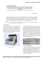
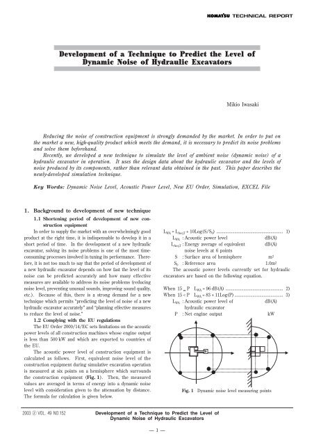
The acoustic power level of construction equipment is
calculated as follows. First, equivalent noise level of the
construction equipment during simulative excavation operation
is measured at six points on a hemisphere which surrounds
the construction equipment (Fig. 1). Then, the measured
values are averaged in terms of energy into a dynamic noise
level with consideration given to the attenuation by distance.
The formula for calculation is given below.
L WA =L AeqT + 10Log(S/S 0 ) ........................................................... 1)
L WA : Acoustic power level dB(A)
L AeqT : Energy average of equivalent dB(A)
noise levels at 6 points
S : Surface area of hemisphere m 2
S 0 : Reference area 1.0m 2
The acoustic power levels currently set for hydraulic
excavators are based on the following equation.
When 15 P L WA = 96 dB(A) ................................................... 2)
When 15 < P L WA = 83 + 11Log(P) ........................................... 3)
L WA : Acoustic power level of dB(A)
hydraulic excavator
P : Net engine output kW
Fig. 1 Dynamic noise level measuring points
2003 w VOL. 49 NO.152
Development of a Technique to Predict the Level of
Dynamic Noise of Hydraulic Excavators
— 1 —

The revised EU Order requires that the acoustic power level
of every construction equipment sold in any of the countries of
the EU in and after January 2006 should be 3 dB(A) lower than
the current regulatory value.
Looking at only the hydraulic excavators manufactured by
Komatsu, more than 30 models, ranging in machine weight from
0.3 ton to 110 tons, are subject to the revised EU Order.
Therefore, it is of urgent necessity for us to reduce their acoustic
power levels. To reduce the acoustic power levels of so many
models within the limited period of time, we must be able to
analyze them speedily and easily. This calls for a new analytical
system which can be used even in the field, unlike such analytical
tools as FEM and SYSNOISE.
2. Conventional noise prediction method and its
problems
2.1 Conventional noise prediction method
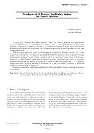
The calculation method that has been most commonly
used to predict the dynamic noise level of a newly-developed
hydraulic excavator is this. From a bench test on the
contribution to noise of each of the components of an existing
machine (q in Fig. 2), it is realized that the noise level of the
muffler (w in Fig. 2) can effectively be reduced. First,
therefore, the amount of reduction in noise level of the muffler
is deducted from the noise level of the newly-developed
machine. Then, the noise levels of all the components are
added up in terms of energy to predict the dynamic noise level
of the newly-developed machine (e in Fig. 2).
This method is also used in the study of measures to
reduce the dynamic noise level of a newly-developed machine.
Namely, the effects of those measures are predicted based on
the actual effects of measures taken with existing machines.
q
Noise level of
existing machine
Muffler
Engine
w
Noise level of
newly-developed machine
Muffler
Engine
e
2.2 Problems in conventional prediction technique
(1) Necessity of studying contributions to noise of individual
components of existing machine
With the conventional prediction method, it is necessary
to study the contribution to the dynamic noise level of each of
the components of an existing machine in order to predict the
dynamic noise level of a newly-developed machine.
The contribution to dynamic noise level of each individual
component is measured by extracting the dynamic noise level of
each component by: q installing a large muffler to reduce the
exhaust sound, w connecting a bellows pipe to keep the suction
sound at a distance from the measuring point, e stopping the
fan operation, r covering the engine with lead urethane, etc.
The man-hours and cost involved in the study of contribution are
a considerable burden on the development of a new machine.
(2) Need for measurement data about existing machines
Predicting the dynamic noise level of a newly-developed
machine requires not only results of studies of contributions
to dynamic noise level of the individual components of existing
machines but also the results of confirmation of the effects of
measures taken with existing machines and various other types
of data, including the drawings of existing machines. Actually,
however, the measurement data that are needed are almost
nonexistent. In many cases, therefore, it is necessary to newly
obtain measurement data with an existing machine or
recalculate using substitute data.
(3) Consideration for differences between new and existing
machines
A newly-developed machine differs from an existing
machine in various respects – the outer panel thickness, engine
speed, sound absorbing material application points, etc. Since
the conventional method analyzes the dynamic noise level of
an existing machine based on its specific conditions, the
conditions of a newly-developed machine are not precisely
reflected in the calculation.
(4) Consideration for frequency range
The conventional noise prediction method focuses on the
level of noise, leaving the frequency range of noise out of
consideration. With this method, therefore, it is difficult to
grasp the frequency range distribution of the sound source and
determine effective sound absorbing materials and optimum
outer panel thickness taking the frequency range into account.
Fan
Fan
Fig. 2 Conventional noise prediction method
2003 w VOL. 49 NO.152
Development of a Technique to Predict the Level of
Dynamic Noise of Hydraulic Excavators
— 2 —

3. Introduction of new noise prediction method
3.1 Features
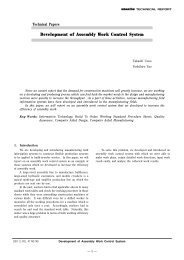
The new noise prediction method calculates the dynamic
noise level of a hydraulic excavator from bench test data about
noise of its engine, muffler, and fan. It takes into account the
transmission loss due to the engine hood, the absorption of
sound by the sound absorbing material, and the attenuation of
sound by distance. The salient features of the new method
are as follows (Fig. 3).
Design procedure
3.2 Premises
(1) The engine compartment is a diffuse sound field.
(2) The open air is a semi-free sound field.
(3) The main sound sources are the engine, muffler, and fan.
(4) The new method cannot be applied when analysis results
are influenced by the directivity of sound.
(5) The engine compartment is assumed as an enclosure
(soundproof cover) (Fig. 4).
Dynamic noise
measuring point
Measure to reduce noise
Reducing
opening area
Setting aimed noise level
Deciding engine compartment
shape and specifications
Engine compartment
(enclosure)
Engine
Changing outer panel
thickness, surface area,
and material density
NO
Changing sound
absorbing material,
thickness, and
application area
NO
NO
Is sound absorbing
capacity sufficient?
YES
Is amount of transmission
loss sufficient?
YES
Calculating sound pressure
of each sound source
Calculating amount of
transmission loss
Calculating sound
absorbing capacity
Calculating sound
attenuation by distance
Calculating dynamic noise level
Is aimed noise
level attained?
END
Fig. 3 Simulation flowchart
YES
(1) Data about existing hydraulic excavators are unnecessary.
Since the new method uses the design data about a newlydeveloped
hydraulic excavator to simulate its noise, it does not
require data about existing hydraulic excavators obtained in
the past, such as their design data or the contribution to noise
of each individual component.
(2) Frequency range is taken into consideration.
Since the new method reflects even the frequency range
of noise in the calculations, it permits analyzing the dynamic
noise level in more detail.
(3) Ease of use.
Since the new method uses an EXCEL file for the
calculations, it is possible to easily grasp the dynamic noise
level of a hydraulic excavator or the effects of measures taken
with the excavator anywhere. All it needs is a personal
computer.
Fig. 4 Noise measuring point
3.3 Principal data used analysis
(All data about newly-developed hydraulic excavator)
(1) Data about covering of engine room compartment
q Material w Thickness e Surface area
r Material density t Opening area
q Opening positions u External dimensions
(2) Characteristics of sound absorbing material
q Material w Thickness e Surface area
r Absorption coefficient
(3) Noise level around components
q Engine sound w Muffler sound e Fan sound
(Results of 1/3 octave band analysis in frequency range 20 Hz
to 20 kHz)
3.4 Main formulas used for calculations
The simulation by the new method is based on the
combination the concepts of the following formulas for
calculations and the analysis taking the frequency range into
account (Fig. 5 and Fig. 6).
Sound level, dB(A)
L p TL
Sound source Transmission loss
sound pressure
Engine compartment
A
Sound absorbing
capacity Sound attenuation
by distance
Fig. 5 Simulation process
L p
L w
TL
A
S
Fig. 6 Simulation scheme
L
Calculated value
r
Measured value
L
2003 w VOL. 49 NO.152
Development of a Technique to Predict the Level of
Dynamic Noise of Hydraulic Excavators
— 3 —

(1) Outdoor noise of indoor sound source 1)
With the engine compartment and open air assumed to
be indoor and outdoor, respectively, the concept of the following
formula was reflected in the simulation. The fourth and fifth
terms represent the sound attenuation by distance in a semifree
sound field.
The average absorption coefficient was obtained from
relevant data supplied by the manufacturer of sound absorbing
materials.
L=L ρ – TL + 10Log(S/A) – 20Log(r) – 8 .................................. 4)
TL = 10Log(ΣS n /(Στ n ·S n )) .......................................................... 5)
A=α · S .......................................................................................... 6)
L ρ : Sound pressure level of indoor sound source (dB)
TL : Average transmission loss (dB)
S : Total indoor surface area (m 2 )
A : Indoor sound absorbing capacity (m 2 )
r : Distance from wall surface to outdoor noise (m)
measuring point
α : Average indoor sound absorption coefficient
S n : Partial area (m 2 )
τ n : Partial transmittance
(2) Effect of enclosure 2)
Assuming the engine compartment as an enclosure
(soundproof cover), the concept of the following formula was
adopted.
The third term in Equation 7) represents the amount of
build-up (increase in sound pressure) due to the enclosure.
L ρ =L W = 10Log(1/S + 4/R)
=L W – 10Log(S) + 10Log[1 + 4(1 – α)/α] ............................ 7)
R=αS/(1 – α) ............................................................................... 8)
L ρ : Sound pressure level at wall surface (dB)
inside enclosure
Lw : Acoustic power level of sound source (dB)
S : Total surface area of enclosure interior (m 2 )
(same as total indoor surface area shown above)
α : Average enclosure sound absorption coefficient
(same as average indoor sound absorption
coefficient shown above)
R : Compartment constant of enclosure interior
(3) Transmission loss 3)
Transmission loss is the ratio of intensity Ii of sound
reaching the wall surface to intensity It of sound penetrating
through the wall, that is, 10Log (Ii/It). In practice, transmission
loss is calculated by the following equation (Table 1).
TL = 18Log(m · f) – 44 .................................................................. 9)
m = n · t ........................................................................................... 10)
m : Surface density (kg/m 2 )
n : Material density (kg/m 3 )
t : Wall thickness (mm)
f : Sound frequency (Hz)
Analyzed frequency range 20 Hz to 20 kHz
Transmission loss
Center
frequency
t
S
20
8000
10000
12500
16000
20000
APc
fc
TLC
Table 1 Transmission loss calculation sheet
Analysis of sound at entire surface
of engine compartment
dB (A)
TL ’
SPHC
1.6
—
-0.8
24.1
47.8
49.5
51.5
53.2
57.6
8028
24.1
3.2
—
4.6
51.5
53.2
54.9
56.9
58.6
63.2
4014
30.1
τ ’
SPHC
1.6
—
1.2E+00
3.9E–03
1.7E–05
1.1E–05
7.2E–06
4.8E–06
3.2
—
3.5E–01
7.2E–06
4.8E–06
3.2E–06
2.1E–06
1.4E–06
SS400P
3.2
2.42
8.3E–01
1.7E–05
1.2E–05
7.7E–06
5.0E–06
3.3E–06
Upper surface
τ · Sn
SPHC hole
1.6 —
3.88 2.59
4.7E+00 2.6E+00
1.5E–02
6.5E–05
4.3E–05
2.8E–05
1.9E–05
2.6E+00
2.6E+00
2.6E+00
2.6E+00
2.6E+00
TL
Total.A
—
9.50
0.7
Transmission loss at coincidence frequency
(4) Coincidence effect 2)
The coincidence effect is the decline in transmission loss
caused by a phenomenon similar to the resonance between
the incoming sound and the wall surface. The frequency at
which this phenomenon occurs is called the coincidence
frequency. It is known that at the coincidence frequency, the
transmission loss is not as large as the law of mass indicates.
f c =C 2 /(1.8 × 10 -3 ·CL · t) ............................................................. 11)
f c : Coincidence frequency (Hz)
C : Sound velocity (m/s)
CL : Longitudinal wave propagation speed (m/s)
(5.0 × 10 3 m/s for steel, 4.0 × 10 3 m/s for concrete)
t : Wall thickness (mm)
(5) Transmission loss at coincidence frequency 4)
The transmission loss at the coincidence frequency was
calculated by using the following equation to improve the
accuracy of simulation.
TL c = 40 – 20Log (10/t) ................................................................ 12)
TL c : Transmission loss at coincidence frequency (dB)
t : Wall thickness (mm)
4. Comparison with measured values
4.1 Prediction of dynamic noise level
The dynamic noise level of each of five different hydraulic
excavators was predicted by using the calculation method
described above, and the calculated values were compared with
the measured values. With the exception of one model which
showed a difference of 2.2 dB (A), we could predict the dynamic
noise level of each of the other four models within a difference
of 1 dB (A). For model C, by predicting its dynamic noise level
before completion, we could recognize the need for suitable
measures to reduce the noise level and thereby shorten the
period of development (Fig. 7).
20dB(A)/graduation
Comparison between calculated
and measured noise levels
5.6
5.6
5.6
5.6
5.6
Measured
value
Calculated
value
Sound source Sound absorbing Transmission Sound attenuation Noise level
sound pressure capacity loss by distance
Fig. 7 Comparison between calculated and measured noise
levels
2003 w VOL. 49 NO.152
Development of a Technique to Predict the Level of
Dynamic Noise of Hydraulic Excavators
— 4 —

4.2 Prediction of effects of measures taken
For model D, various measures to reduce its dynamic
noise level were studied by using the new noise prediction
method. As a result, we could judge the effects of those
measures before they were taken.
(1) Planned measures to reduce dynamic noise level
q Blocking some of the openings in the hood
w Increasing the volume of sound absorbing material
e Increasing the thickness of sound absorbing material
r Lowering the engine speed
(2) Result of confirmation
An analysis by the new noise prediction method showed
that planned measure q would be the most effective of the
four planned measures shown above. Therefore, we took that
measure in order to confirm the accuracy of prediction.
(1) Content of measure taken:
Blocking some of the openings in the hood (The openings
blocked are in the portion indicated by oblique lines in Fig. 8.)
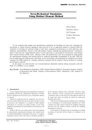
5. Implementation of experiment with model
With the aim of further improving the accuracy of
simulation by the new noise prediction method and isolating
problems in the method, we carried out an experiment using
a model in a semi-anechoic room of Shiga Prefectural University
(Fig. 9 and Fig. 10).
Fig. 9 Scene of experimentation with model (1)
Fig. 8 Measure taken with the engine hood
(2) Result of confirmation
The predicted noise level was 72.2 dB (A) and the measured
noise level was 71.9 dB (A). Thus, it was confirmed that the new
noise prediction method could simulate even results of measures
with a high degree of accuracy.
Fig. 10 Scene of experimentation with model (2)
5.1 Conditions
Sound source : YAMAHA MS60S
Specimen box : 0.7m × 0.8m × 0.4m, SPHC t1.6
Semi-anechoic room : 5.0m × 5.0m × 3.0m(H)
Noise produced : Pink noise Generator: RION SA28
Noise meter : RION precision noise meter NA27
Analyzer
: ONO SOKKI DS9000 Series
5.2 Method
Assuming the speaker as the engine and the specimen box
as the engine compartment, their dimensions were made the
same in proportion as a 15 ton class hydraulic excavator. The
noise level around the specimen box was obtained from the noise
level around the speaker. With the specimen box placed at the
center of a virtual hemisphere in the test room, the dynamic
noise level was measured by the method specified in ISO 3744
(1994) (calculation of acoustic power level of sound source by
sound pressure method) to check the validity of the new noise
prediction technique. The main methods used are shown below.
(1) Transmission loss
Sound pressure level was measured inside and outside the
specimen box.
(2) Sound absorbing capacity
Sound pressure level inside the specimen box with and
without the sound absorbing material (PET) was measured.
2003 w VOL. 49 NO.152
Development of a Technique to Predict the Level of
Dynamic Noise of Hydraulic Excavators
— 5 —

5.3 Results
In each calculation process, the difference between
calculated and measured values, including those of noise level,
was within 2 dB(A). It was found that the difference between
calculated and measured values of transmission loss was the
largest. In the future, it is necessary to carry out many
experiments and formulate an experimental formula so that the
new noise prediction technique can simulate the dynamic noise
level more accurately (Fig. 11).
Comparison between calculated and measured values
dB(A)
Measured
value
Calculated
value
Introduction of the writer
Mikio Iwasaki
Entered Komatsu in 1993. Currently
working in Test Engineering Center,
Development Division, Komatsu.
[A few words from the writer]
The advances in the field of CAE are so fast that almost
everything can be predicted fairly accurately on the drawing board.
However, truth lies only in principles, rules, workshops, actual
things, realities. I think that this must be remembered when
making simulations of any kind.
Sound source Sound absorbing Transmission Sound attenuation Noise level
sound pressure capacity loss by distance
6. Conclusion
Fig. 11 Results of experiment with model
At present, the noise levels of almost all components of
construction equipment are evaluated by sound pressure levels
measured at several points of each of those components. In the
future, we would like to improve the accuracy of calculation by
the new noise prediction technique and shorten the period of
development of new hydraulic excavators by grasping the level
of their noise in terms of the acoustic power level and reflecting
the value in the simulation by the new technique. I wish to
express my heartfelt thanks to the people of Shiga Prefectural
University for their generous cooperation in the verification
experiment.
References
1) Antipollution Technology and Law (Noise Edition),
Maruzen Co., Ltd., p. 133
2) Kazuhiro Shiraki: Prevention of Noise and Simulation,
Oyogijutsu Shuppan Co., Ltd., p. 229
3) Acoustical Materials Association of Japan: Handbook on
Measures against Noise and Vibration, Gihodo Shuppan
Co., Ltd.
4) WattersB.G., J.Acous.SocAm.31(7)898-911, 1959
2003 w VOL. 49 NO.152
Development of a Technique to Predict the Level of
Dynamic Noise of Hydraulic Excavators
— 6 —