Atomic Force Microscopy - KIP - Ruprecht-Karls-Universität Heidelberg
Atomic Force Microscopy - KIP - Ruprecht-Karls-Universität Heidelberg
Atomic Force Microscopy - KIP - Ruprecht-Karls-Universität Heidelberg

Create successful ePaper yourself
Turn your PDF publications into a flip-book with our unique Google optimized e-Paper software.
<strong>Ruprecht</strong>-<strong>Karls</strong> <strong>Universität</strong> <strong>Heidelberg</strong><br />
Kirchhoff-Institut für Physik<br />
Im Neuenheimer Feld 227<br />
69120 <strong>Heidelberg</strong><br />
<strong>Atomic</strong> <strong>Force</strong> <strong>Microscopy</strong><br />
Instructions to the lab course<br />
Last revised on November 21, 2013
Supervisors:<br />
Jochen Vogt, <strong>KIP</strong>, room 2.301, phone 06221-549892<br />
e-mail: jochen.vogt@kip.uni-heidelberg.de<br />
Michael Sendner, <strong>KIP</strong>, room 2.301, phone 06221-549892<br />
e-mail: sendner@kip.uni-heidelberg.de<br />
Olaf Skibbe, <strong>KIP</strong>, room 1.310, phone 06221-549890,<br />
e-mail: olaf.skibbe@uni-heidelberg.de.<br />
Location of practical course:<br />
<strong>KIP</strong>, INF 227, room 2.215
Preliminary Note<br />
The aim of this practical course experiment is to<br />
give the students an insight into the technique of<br />
scanning probe microscopy (SPM) with an atomic<br />
force microscope (AFM) taken as example. Since this<br />
kind of microscopy is widely-used in research areas<br />
which deal with structures on the nanometer scale, it<br />
might serve as a prototypic example for an up-to-date<br />
method in surface science. At the same time the used<br />
device is sufficiently simple to be used by students in<br />
the frame-set of a lab course without the permanent<br />
presence of the supervisor.<br />
The students should be familiar with chapter 1<br />
to 3 of this tutorial prior to the beginning of the<br />
experiment. They should focus on the underlying<br />
principles of the physics of the AFM. In addition<br />
to this instructions, a large variety of information<br />
about the subject and related methods is available for<br />
instance in the world wide web. The list of questions<br />
and tasks in the preparation section 2.3 should be<br />
answered in advance to the lab course.<br />
Chapter 4 deals with the instrumental details for<br />
the lab course and some additional information about<br />
problem solving. This chapter is not necessary to<br />
read in advance.<br />
This instructions are work in progress, so every hint<br />
on errors or on possible improvements is appreciated.<br />
3
Contents<br />
1 Introduction 5<br />
1.1 Scanning Probe <strong>Microscopy</strong> . . . . . . . . . . . . . . . . . . . . . . . . . . . . . . . . . . . . 5<br />
1.2 The Scanning <strong>Force</strong> Microscope . . . . . . . . . . . . . . . . . . . . . . . . . . . . . . . . . . 5<br />
2 Basics 6<br />
2.1 Theoretical Principles . . . . . . . . . . . . . . . . . . . . . . . . . . . . . . . . . . . . . . . 6<br />
2.1.1 Van der Waals interaction . . . . . . . . . . . . . . . . . . . . . . . . . . . . . . . . . 6<br />
2.1.2 Approaching the surface (<strong>Force</strong> distance behavior) . . . . . . . . . . . . . . . . . . . 7<br />
2.1.3 Operation Modes . . . . . . . . . . . . . . . . . . . . . . . . . . . . . . . . . . . . . . 7<br />
2.2 Operation Principles . . . . . . . . . . . . . . . . . . . . . . . . . . . . . . . . . . . . . . . . 9<br />
2.2.1 Optics . . . . . . . . . . . . . . . . . . . . . . . . . . . . . . . . . . . . . . . . . . . . 9<br />
2.2.2 Feedback control . . . . . . . . . . . . . . . . . . . . . . . . . . . . . . . . . . . . . . 9<br />
2.3 Preparation Tasks . . . . . . . . . . . . . . . . . . . . . . . . . . . . . . . . . . . . . . . . . 10<br />
3 Experiments and Evaluation 11<br />
3.1 P and I Values . . . . . . . . . . . . . . . . . . . . . . . . . . . . . . . . . . . . . . . . . . . 11<br />
3.2 Tip Characterisation and Limitations of the AFM . . . . . . . . . . . . . . . . . . . . . . . 11<br />
3.3 Samples . . . . . . . . . . . . . . . . . . . . . . . . . . . . . . . . . . . . . . . . . . . . . . . 12<br />
3.3.1 Pre-pressed and burned CD/DVD . . . . . . . . . . . . . . . . . . . . . . . . . . . . 12<br />
3.3.2 Nano Lattice . . . . . . . . . . . . . . . . . . . . . . . . . . . . . . . . . . . . . . . . 12<br />
3.3.3 CCD-Chip . . . . . . . . . . . . . . . . . . . . . . . . . . . . . . . . . . . . . . . . . . 12<br />
3.3.4 Additional Samples . . . . . . . . . . . . . . . . . . . . . . . . . . . . . . . . . . . . . 12<br />
3.4 <strong>Force</strong>-Distance Curve . . . . . . . . . . . . . . . . . . . . . . . . . . . . . . . . . . . . . . . . 12<br />
4 Technical Support 15<br />
4.1 Start-up . . . . . . . . . . . . . . . . . . . . . . . . . . . . . . . . . . . . . . . . . . . . . . . 15<br />
4.2 Parameters for Image Mode . . . . . . . . . . . . . . . . . . . . . . . . . . . . . . . . . . . . 16<br />
4.2.1 Scan Controls: . . . . . . . . . . . . . . . . . . . . . . . . . . . . . . . . . . . . . . . 16<br />
4.2.2 Feedback Controls . . . . . . . . . . . . . . . . . . . . . . . . . . . . . . . . . . . . . 17<br />
4.2.3 Channel 1, 2 and 3 . . . . . . . . . . . . . . . . . . . . . . . . . . . . . . . . . . . . . 17<br />
4.3 Parameters for <strong>Force</strong> Mode . . . . . . . . . . . . . . . . . . . . . . . . . . . . . . . . . . . . 18<br />
4.3.1 Main Control . . . . . . . . . . . . . . . . . . . . . . . . . . . . . . . . . . . . . . . . 18<br />
4.3.2 Channel 1, 2 and 3 . . . . . . . . . . . . . . . . . . . . . . . . . . . . . . . . . . . . . 19<br />
4.4 Trouble Shooting . . . . . . . . . . . . . . . . . . . . . . . . . . . . . . . . . . . . . . . . . . 19<br />
4.5 Poor Image Quality . . . . . . . . . . . . . . . . . . . . . . . . . . . . . . . . . . . . . . . . 20<br />
Bibliography 21<br />
4
1 Introduction<br />
1.1 Scanning Probe <strong>Microscopy</strong><br />
The method of scanning probe microscopy (SPM)<br />
was developed in 1981 by Binnig and Rohrer with<br />
the invention of the scanning tunnelling microscope<br />
(STM) [1, 2]. This technique exploits the fact that<br />
a tunnelling current through a potential barrier of<br />
the width d is proportional to e −d (provided a constant<br />
and final height of the potential barrier). With<br />
a sharp tip close to a surface, one can measure by<br />
applying a voltage between tip and surface the tunnelling<br />
current between the tip and the surface atoms<br />
in the vicinity of the tip. The strong dependence of<br />
the current from the distance d allows one to detect<br />
changes in distance on a sub-atomic scale. By moving<br />
the tip parallel to the surface, the height of the surface<br />
can be scanned. To control such distances, electromechanical<br />
devices of high precision are required.<br />
This task is commonly solved by piezo-ceramics. For<br />
an understanding of the images generated this way<br />
one has to take into account that the tunnelling current<br />
is also a function of the chemical properties of<br />
the surface. For a more detailed description and<br />
discussion of STM see e.g. [3, 4].<br />
The scanning tunnelling microscope is (in general)<br />
restricted to conducting materials. The surfaces of insulators,<br />
structures in liquids and biological samples<br />
can be imaged non destructive with high resolution by<br />
the atomic force microscope (AFM) (also often scanning<br />
force microscope, SFM), which was developed<br />
in 1986 by Binnig, Quate and Gerber [5].<br />
1.2 The Scanning <strong>Force</strong><br />
Microscope<br />
This subsections is mainly taken from [6] and slightly<br />
adapted.<br />
The design and development of the scanning force<br />
microscope (SFM) (or frequently called atomic force<br />
microscope AFM) is very closely connected with that<br />
of scanning tunnelling microscopy. The central component<br />
of these microscopes is basically the same. It is<br />
a fine tip positioned at a characteristic small distance<br />
from the sample. The height of the tip above the<br />
sample is adjusted by piezoelectric elements. In STM<br />
the tunneling current gives the information about<br />
the surface properties, whereas in SFM the forces<br />
between the tip and the surface are used to gain this<br />
information. The images are taken by scanning the<br />
sample relative to the probing tip and measuring the<br />
deflection of the cantilever as a function of lateral<br />
position. The height deflection is measured by optical<br />
techniques, which will be described in more detail<br />
later.<br />
A rich variety of forces can be sensed by scanning<br />
force microscopy. In the non-contact mode (of distances<br />
greater than 1 nm between the tip and the<br />
sample surface), van der Waals, electrostatic, magnetic<br />
or capillary forces produce images, whereas in<br />
the contact mode, repulsion forces take the leading<br />
role. Because its operation does not require a current<br />
between the sample surface and the tip, the SFM<br />
can move into potential regions inaccessible to the<br />
scanning tunnelling microscope (STM), for example<br />
samples which would be damaged irreparably by the<br />
STM tunnelling current. Insulators, organic materials,<br />
biological macromolecules, polymers, ceramics<br />
and glasses are some of the many materials which<br />
can be imaged in different environments, such as in<br />
liquids, under vacuum, and at low temperatures.<br />
In the non-contact mode one can obtain a surface<br />
analysis with a true atomic resolution. However, in<br />
this case the sample has to be prepared under ultrahigh<br />
vacuum (UHV) conditions. Recently, it has been<br />
shown that in the tapping mode (a modified noncontact<br />
mode) under ambient conditions it is possible<br />
to observe, similar as in STM investigations, single<br />
vacancies or their agglomeration [7]. Additionally, a<br />
non-contact mode has the further advantage over the<br />
contact mode that the surface of very soft and rough<br />
materials is not influenced by frictional and adhesive<br />
forces as during scanning in contact mode, i.e. the<br />
surface is not “scratched”.<br />
5
2 Basics<br />
Figure 2.1: Van der Waals potential U between two<br />
atoms. d r is the critical distance above which the transit<br />
time effects weaken the interaction. (Taken from [6].)<br />
Figure 2.2: Schematic illustration of the three described<br />
interaction cases in the text: a) sphere with half-space,<br />
b) two spheres and c) sphere (Tip) with half-space.<br />
2.1 Theoretical Principles<br />
This section and subsections are mainly taken from<br />
[6] and slightly adapted.<br />
2.1.1 Van der Waals interaction<br />
As already mentioned above, van der Waals forces<br />
lead to an attractive interaction between the tip on<br />
the spring and the sample surface. Figure 2.1 shows<br />
schematically the van der Waals potential between<br />
two atoms. The potential can be described in a<br />
simpler classical picture as the interaction potential<br />
between the time dependent dipole moments of the<br />
two atoms. Although the centres of gravity of the<br />
electronic charge density and the charge of the nucleus<br />
are exactly overlapping on a time average, the<br />
separation of the centres of gravity is spatially fluctuating<br />
in every moment. These statistical fluctuations<br />
give rise to an transient dipole moment of the particle<br />
while it might be in average unpolarised. The<br />
dipole moment of an atom can again induce a dipole<br />
moment in the neighbouring atom and the induced<br />
dipole moment acts back on the first atom. This<br />
creates a dipole-dipole interaction on basis of the fluctuating<br />
dipole moments. This interaction decreases<br />
with d −6 in the case of small distances d (Lenard<br />
Jones potential). At larger distances, the interaction<br />
potential decreases more rapidly (d −7 ). This arises<br />
from the fact that the interaction between dipole<br />
moments occurs through the exchange of virtual photons,<br />
as indicated in figure 2.1. If the transit time of<br />
the virtual photon between atom 1 and 2 is longer<br />
than the typical fluctuation time of the instantaneous<br />
dipole moment, the virtual photon weakens the interaction.<br />
This range of the van der Waals interaction<br />
is therefore called retarded, whereas that at short<br />
distances is unretarded.<br />
The scanning force microscope is not based on<br />
the interaction of individual atoms only. Both the<br />
sample and the tip are large in comparison to the<br />
distance. In order to obtain their interaction, all<br />
forces between the atoms of both bodies need to be<br />
integrated. The result of this is known for simple<br />
bodies and geometries. In all cases, the summation<br />
leads to a weaker decrease of the interaction. Some<br />
examples:<br />
• Single atom over half space<br />
A single atom at a distance d relative to the halfspace<br />
(see figure 2.2 a)) leads to an interaction<br />
potential of<br />
U = − Cπρ<br />
6<br />
1<br />
d 3 (2.1)<br />
where C is the interaction constant of the van<br />
der Waals potential and ρ the density of the<br />
solid. C is basically determined by the electronic<br />
polarisability of the atoms in the half-space and<br />
of the single atom.<br />
• Two spheres<br />
If one has two spheres with radii R 1 and R 2 at<br />
distance d (distance between sphere surfaces, as<br />
shown in figure 2.2 b)) one obtains an interaction<br />
potential of<br />
U = − HR 1R 2 1<br />
6(R 1 + R 2 ) d<br />
(2.2)<br />
where H is the so called Hamaker constant. It<br />
can be defined for a van der Waals body-body<br />
interaction as H = π 2 × C × ρ 1 × ρ 2 where ρ 1<br />
and ρ 2 are the number of atoms per unit volume<br />
in two interacting bodies and C is the coefficient<br />
in the particle-particle pair interaction [8]. It<br />
6
2.1 Theoretical Principles<br />
to bend in the opposite direction as a result of a<br />
repulsing interaction (“b-c”). In the range (“b-c”)<br />
the position of the laser beam on both quadrants,<br />
which is proportional to the force, is a linear function<br />
of distance. On reversal this eristic shows a hysteresis.<br />
This means that the cantilever loses contact with the<br />
surface at a distance (point “d”) which is much larger<br />
than the distance on approaching the surface (point<br />
“a”).<br />
Figure 2.3: Schematic representation of the effect of<br />
the van der Waals interaction potential on the vibration<br />
frequency of the spring with tip. As the tip approaches<br />
the surface, the resonance frequency of the leaf spring is<br />
shifted. (Taken from [6].)<br />
is material specific and essentially contains the<br />
densities of the two bodies and the interaction<br />
constant C of the van der Waals potential.<br />
• Sphere over half-space<br />
If a sphere with the radius R has a distance d<br />
from a half-space (see figure 2.2 c)), an interaction<br />
potential of<br />
U = − HR<br />
6<br />
1<br />
d<br />
(2.3)<br />
is obtained from Eq. (2.2). This case describes<br />
the geometry in a scanning force microscope<br />
best and is most widely used. The distance dependence<br />
of the van der Waals potential thus<br />
obtained is used analogously to the distance dependence<br />
of the tunnel current in a scanning<br />
tunnelling microscope to achieve a high resolution<br />
of the scanning force microscope. However,<br />
since the distance dependence is much weaker,<br />
the sensitivity of the scanning force microscope<br />
is lower.<br />
Figure 2.4: Cantilever force as a function of the tip–<br />
sample distance. (Taken from [6].)<br />
2.1.3 Operation Modes<br />
Many AFM operation modes have appeared for special<br />
purpose during the further development of AFM.<br />
These can be classified into static modes and dynamic<br />
2.1.2 Approaching the surface (<strong>Force</strong><br />
distance behavior)<br />
For large distances between the tip and the sample<br />
the bending of the cantilever by attractive forces is<br />
negligible. After the cantilever is brought closer to<br />
the surface of the sample (point “a” Figure 2.4) the<br />
van der Waals forces induce a strong deflection of the<br />
cantilever and, simultaneously, is moving towards the<br />
surface. This increases the forces on the cantilever,<br />
which is a kind of positive feedback and brings the<br />
cantilever to a direct contact with the sample surface<br />
(point “b”). However, when the cantilever is brought<br />
even closer in contact to the sample, it actually begins<br />
Figure 2.5: <strong>Force</strong>-distance curve. Classification of the<br />
AFM operation modes within the working regime of the<br />
van der Waals potential.<br />
7
2 Basics<br />
Figure 2.6: Resonance curves of the tip without and<br />
with a van der Waals potential. The interaction leads to a<br />
shift ∆ω of the resonance frequency with the consequence<br />
that the tip excited with the frequency ω m has a vibration<br />
amplitude a(ω) attenuated by ∆a. (Taken from [6].)<br />
modes. Another classification could be contact, noncontact<br />
and intermittent-contact which is reclined to<br />
the working regimes (see figure 2.5).<br />
Here the three commonly used techniques, namely<br />
static mode (contact mode) and dynamic mode (noncontact<br />
mode and tapping mode) will be shortly described.<br />
Further information can be found in textbooks<br />
or review articles.<br />
Contact mode/static mode<br />
In contact mode the tip scans the sample in close<br />
contact with the surface and the force acting on the<br />
tip is repulsive of the order of 10 −9 N. This scanning<br />
mode is very fast, but has the disadvantage that additionally<br />
to the normal force frictional forces appear<br />
which can be destructive and damage the sample<br />
or/and the tip.<br />
Constant height mode: This mode is particular<br />
suited for very flat samples. The height of the tip<br />
is set constant and by scanning the sample only the<br />
deflection of the cantilever is detected by an optical<br />
system (described in 2.2.1) and gives the topographic<br />
information.<br />
Constant force mode: In this mode the force acting<br />
on the cantilever, i.e. the deflection, is set to a<br />
certain value and changes in deflection can be used as<br />
input for the feedback circuit that moves the scanner<br />
up and down. The system is therefore responding<br />
to the changes in height by keeping the cantilever<br />
deflection constant. The motion of the scanner gives<br />
the direct information about the topography of the<br />
sample. The scanning time is limited by the response<br />
of the feedback circuit and therefore not as fast as<br />
the constant height mode.<br />
Dynamic Modes<br />
The dynamic operation method of a scanning force<br />
microscope has proved to be particularly useful. In<br />
this method the normal force constant of the van der<br />
Waals potential, i.e. the second derivative of the potential,<br />
is exploited. This can be measured by using<br />
a vibrating tip (Figure 2.3). If a tip vibrates at a distance<br />
d, which is outside the interaction range of the<br />
van der Waals potential, then the vibration frequency<br />
and the amplitude are only determined by the spring<br />
constant k of the cantilever. This corresponds to a<br />
harmonic potential. When the tip comes into the<br />
interaction range of the van der Waals potential, the<br />
harmonic potential and the interaction potential are<br />
superimposed thus changing the vibration frequency<br />
and the amplitude of the spring.<br />
This is described by modifying the spring constant<br />
k of the spring by an additional contribution f of<br />
the van der Waals potential. As a consequence, the<br />
vibration frequency is shifted to lower frequencies as<br />
shown in Figure 2.6. ω 0 is the resonance frequency<br />
without interaction and ∆ω is the frequency shift to<br />
lower values. If an excitation frequency of the tip of<br />
ω m > ω 0 is selected and kept constant, the amplitude<br />
of the vibration decreases as the tip approaches<br />
the sample, since the interaction becomes increasingly<br />
stronger. Thus, the vibration amplitude also<br />
becomes a measure for the distance of the tip from<br />
the sample surface. If a spring with a low damping<br />
Q −1 is selected, the resonance curve is steep and the<br />
ratio of the amplitude change for a given frequency<br />
shift becomes large. In practice, small amplitudes<br />
(approx. 1 nm) in comparison to distance d are used<br />
to ensure the linearity of the amplitude signal. With<br />
a given measurement accuracy of 1 %, however, this<br />
means the assembly must measure deflection changes<br />
of 0.001 nm, which is achieved most simply by a laser<br />
interferometer or optical lever method.<br />
Non-contact mode: Since in the non-contact<br />
regime the force between the tip and the surface<br />
is of the order of 10 −12 N and therefore much weaker<br />
than in the contact regime the tip has to be driven in<br />
the dynamic mode, i.e. the tip is vibrated near the<br />
surface of the sample and changes in resonance frequency<br />
or amplitude are detected and used as input<br />
for the feedback circuit. In this case the resonance<br />
frequency or the amplitude are held constant by moving<br />
the sample up and down and recording directly<br />
the topography of the sample.<br />
8
2.2 Operation Principles<br />
Tapping mode: Tapping mode is an intermittentcontact<br />
mode. In general it is similar to the noncontact<br />
mode described before, except that the tip is<br />
brought closer to the surface and taps the surface at<br />
the end of his oscillation. This mode is much more<br />
sensitive than the non-contact mode and in contrary<br />
to contact mode no frictional forces appear which<br />
can alter the tip or the surface. Therefore this is the<br />
mode of choice for the most experiments and during<br />
the lab course.<br />
2.2 Operation Principles<br />
variation in the laser power P . Hence the normalised<br />
difference is used, which is only dependent of δ:<br />
P A − P B<br />
P A + P B<br />
= δ 3S 2<br />
Ld . (2.4)<br />
The “lever amplification” ∆d/δ = 3S 2 /L is about a<br />
factor of one thousand. On the basis of this kind<br />
of technique one is able to detect changes in the<br />
position of a cantilever of the order of 0.001 nm. These<br />
changes are used as input signal for the feedback<br />
system described below.<br />
2.2.1 Optics<br />
The main electronic components of the SFM are the<br />
same as for the STM, only the topography of the<br />
scanned surface is reconstructed by analysing the deflection<br />
of the tip at the end of a spring. Today, the<br />
interferometrical and the optical lever method dominate<br />
commercial SFM apparatus. The most common<br />
method for detecting the deflection of the cantilever<br />
is by measuring the position of a reflected laser-beam<br />
on a photosensitive detector. The principle of this<br />
optical lever method is presented in Figure 2.7. Without<br />
cantilever displacement, both quadrants of the<br />
photo diode (A and B) have the same irradiation<br />
P A = P B = P/2 (P represents the total light intensity).<br />
The change of the irradiated area in the<br />
quadrants A and B is a linear function of the displacement.<br />
Figure 2.8: Schematic illustration of the feedback loop<br />
and the optical system.<br />
Figure 2.7: The amplification of the cantilever motion<br />
through the optical lever arm method. Optical laser path<br />
in the standard AFM set-up. (Taken from [6].)<br />
Using the simple difference between P A and P B<br />
gives therefore the necessary information on the deflection<br />
but in this case one cannot distinguish between<br />
the displacement δ of the cantilever and the<br />
2.2.2 Feedback control<br />
For the realisation of a scanning force microscope,<br />
the force measurement must be supplemented by a<br />
feedback control (see figure 2.8), in analogy to the<br />
scanning tunnelling microscope. The controller keeps<br />
the amplitude or the resonance frequency of the vibration<br />
of the cantilever (the tip), and thus also the<br />
distance, constant. During scanning the feedback controller<br />
retracts the sample with the scanner of a piezoelectric<br />
ceramic or shifts towards the cantilever until<br />
the vibration amplitude or frequency has reached the<br />
setpoint value again. The scanning force micrographs<br />
thus show areas of constant effective force constant.<br />
If the surface is chemically homogeneous and if only<br />
the van der Waals forces act on the tip, the SFM<br />
image shows the topography of the surface.<br />
9
2 Basics<br />
2.3 Preparation Tasks<br />
• What are the underlying principles of AFM?<br />
What forces act between tip and sample? What<br />
does the corresponding potential look like?<br />
• Briefly describe the experimental setup of the<br />
AFM. How is the information on the sample<br />
topography obtained?<br />
• What operation modes can be chosen? Briefly<br />
describe the different modes and their advantages/disadvantages.<br />
• During this lab course we will only use the tapping<br />
mode. How does this mode work in detail?<br />
(How is the resonance curve (amplitude vs. frequency)<br />
modified when the tip approaches the<br />
surface? Which parameter of the oscillation provides<br />
information on the height profile when the<br />
excitation frequency is kept constant?<br />
• In our case the system keeps the distance between<br />
tip and sample surface constant. This is done<br />
by piezo-materials and a PID controller. How<br />
can piezo-materials be used in motion systems?<br />
What is a PID controller?<br />
• What’s the resolution of an AFM and how is it<br />
limited? How is the image influenced by the tip<br />
shape?<br />
• What are the advantages of an AFM? E.g. in<br />
comparison with a SEM or STM?<br />
• Get information from the internet on how the<br />
data is stored on a CD (How are 0 and 1 realized?<br />
How is the data stored? Keyword: Eightto-Fourteen-Modulation).<br />
You can find a nice<br />
overview at: http://rz-home.de/~drhubrich/<br />
CD.htm#code<br />
• In the last part of the lab course a force-distance<br />
curve will be measured. How does the deflection<br />
of the tip (proportional to the force) change when<br />
it approaches the surface? What difference do<br />
you expect for retracting the tip?<br />
10
3 Experiments and Evaluation<br />
Goal of these experiments is to learn about the<br />
basic functioning and possibilities of the atomic force<br />
microscope. The structure of two calibration grids<br />
and different surfaces will be observed and quantified.<br />
A detailed description on how to operate the microscope<br />
and the meaning of the different scan parameters<br />
is given in chapter 4. It is essential that<br />
the correct profile (afmprak2) is loaded. In case of<br />
problems, have a look at sections 4.1 and 4.4.<br />
Important: All measurements for the whole<br />
lab course should be performed with the maximum<br />
resolution of 512 x 512 points and a scan<br />
rate of 1 Hz.<br />
It takes quite some time to record an AFM image<br />
but you can and you should use this time to do your<br />
evaluation.<br />
3.1 P and I Values<br />
Start the microscope as described in chapter 4.1 and<br />
take a screenshot of the resonance curve. As first<br />
sample use the calibration grid TGZ02 (see figure<br />
3.3).<br />
Vary the values of the proportional gain P and<br />
the integral gain I, while imaging the surface of the<br />
calibration grid in Dual Trace Mode. Try to find<br />
optimal values for both parameters. Take pictures for<br />
the optimal values you found and for too high and<br />
too low values for I, respectively.<br />
Images that have to be taken:<br />
• Screenshot of the resonance curve (old tip)<br />
• Dual Trace Mode for optimal P and I values<br />
• Dual Trace Mode for too high I values<br />
• Dual Trace Mode for too low I values<br />
Discuss the effect of high/low proportional and integral<br />
gain with respect to the image quality versus a<br />
reliable height measurement.<br />
Important: The P and I values have to<br />
be checked and potentially adjusted for every<br />
new sample.<br />
3.2 Tip Characterisation and<br />
Limitations of the AFM<br />
In order to experience the limitations of the AFM<br />
two calibration grids with different step heights are<br />
measured.<br />
Important: All measurements for the<br />
whole lab course should be performed with<br />
a resolution of 512 x 512 points and a scan<br />
rate of 1 Hz.<br />
Start with calibration grid TGZ02 and take one<br />
image with the scanning direction perpendicular to<br />
the steps, then change the scanning angle about 90 ◦<br />
and take a second image with scanning direction<br />
parallel to the steps. Describe what you observe<br />
for the different scanning directions and discuss the<br />
reason for your observation.<br />
Repeat the measurement with scanning direction<br />
perpendicular to the steps for the calibration grid<br />
TGZ01 (don’t forget to readjust the P and I values).<br />
After you finished all measurements with the old<br />
tip, determine again the resonance curve and take a<br />
screenshot.<br />
After that a new tip will be given to you by your<br />
supervisor. First take a screenshot of the new resonance<br />
curve and then investigate again the grid<br />
TGZ01 (perpendicular scanning direction).<br />
All images that have to be taken for this part of<br />
the lab course are listed below:<br />
• TGZ02 scanning direction perpendicular to the<br />
steps (10µm x 10µm) (old tip)<br />
• TGZ02 scanning direction parallel to the steps<br />
(10µm x 10µm) (old tip)<br />
• TGZ01 scanning direction perpendicular to the<br />
steps (10µm x 10µm) (old tip)<br />
• Screenshot of the resonance curve (old tip)<br />
• Screenshot of the resonance curve (new tip)<br />
• TGZ01 scanning direction perpendicular to the<br />
steps (10µm x 10µm) (new tip)<br />
To analyse the grid structure use the three images<br />
with perpendicular scanning direction and determine<br />
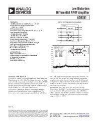
step width w, step height h and the angle ϕ (see<br />
figure 3.1).<br />
Make five cross sections perpendicular to the steps<br />
and measure each value. Calculate the mean value<br />
and the standard deviation.<br />
Compare the values for the step height and the step<br />
width to the values given by the manufacturer and<br />
discuss the relative errors comparing the two grids<br />
measured with the old tip.<br />
11
3 Experiments and Evaluation<br />
h<br />
φ<br />
w<br />
Figure 3.1: Values to be determined in the evaluation<br />
light on the sample. In the optical microscope the<br />
colors are not clearly visible but there are bright and<br />
dark stripes. The geometric properties of the stripes<br />
change continously from the dark to the bright side.<br />
Determine to which end of the rainbow the dark and<br />
the bright stripes correspond respectively. Choose<br />
two different stripes (one from the dark and one from<br />
the bright side) and take one image of each.<br />
Images:<br />
Second, compare the values obtained for TGZ01<br />
with the new and the old tip. Discuss these results<br />
in terms of tip radius, shape and inclination.<br />
In addition compare the resonance curves with<br />
respect to the shape and the resonance position, use<br />
as well the resonance curve determined in 3.1. Are<br />
there any changes/differences?<br />
3.3 Samples<br />
3.3.1 Pre-pressed and burned<br />
CD/DVD<br />
In order to estimate the capacity of a CD, a sample<br />
of a pre-pressed CD-ROM has been prepaired wetchemically<br />
for you. Take an overview image (10µm x<br />
10µm), think about the best scanning direction (parallel<br />
or perpendicular to the spiral lines) to determine<br />
the length of a pit.<br />
• Pre-pressed CD surface with best scanning direction<br />
(10µm x 10µm)<br />
Measure (with a ruler) the area of the CD where<br />
data is stored. From this area you can calculate the<br />
length of the total track using the distance between<br />
two spiral lines. Determine the length of the shortest<br />
pit and compare this to literature data. How is the<br />
digital information (1 and 0) stored on a CD and<br />
how many channelbits are coded in the shortest pit?<br />
Furthermore, try to estimate the capacity of a CD<br />
using your results. (This might be helpful: http:<br />
//rz-home.de/~drhubrich/CD.htm#Code)<br />
Now prepare a sample of a burned CD surface on<br />
your own by retracting a small square of the dye layer.<br />
Again take an overview image (10µm x 10µm).<br />
• Burned CD surface with best scanning direction<br />
(10µm x 10µm)<br />
What are the differences between the two samples<br />
(only qualitatively)? What are the reasons for that?<br />
3.3.2 Nano Lattice<br />
The areas with the nano lattices are visible with<br />
bare eye as rainbow-coloured stripes when reflecting<br />
• Stripe from dark side (approx. 1.5µm x 1.5µm)<br />
• Stripe from bright side (approx. 1.5µm x 1.5µm)<br />
Characterize the structures you find (depths, diameter,<br />
distance between features) and compare the<br />
values obtained for the two different stripes. How<br />
do the geometric dimensions correlate to the color<br />
impression?<br />
Imagine the lattice you observed being smaller<br />
(with a lattice constant of a few Ångstrom) and the<br />
lattice points being occupied by atoms of the same<br />
species. Which surface of an fcc crystal is then represented?<br />
Hint: Try to remember how the low-index<br />
surfaces fcc(100), fcc(110) and fcc(111) look like!<br />
3.3.3 CCD-Chip<br />
Important: The CCD-chip is a very high sample.<br />
Make sure you raise the AFM tip high<br />
enough before changing the sample!<br />
This sample is the CCD-chip of an old digital camera.<br />
Take an image of the surface.<br />
• CCD-Chip (10µm x 10µm)<br />
Measure (with a ruler) the size of the whole chip. Determine<br />
the size of one pixel from your measurement.<br />
Calculate the megapixels of this camera. When you<br />
do this, remember that the camera can take color<br />
pictures! How is the color information obtained?<br />
3.3.4 Additional Samples<br />
You are encouraged to bring along some samples of<br />
your own. The size of the samples should not exceed<br />
10 mm ×10 mm ×4 mm and the structures should not<br />
be higher than 500 nm.<br />
3.4 <strong>Force</strong>-Distance Curve<br />
Use a mica surface to get a force-distance curve for<br />
approaching and retracting the surface. First you<br />
determine again the resonance curve for the tip you<br />
are currently using. Then start imaging the surface<br />
in tapping mode and switch during acquisition into<br />
the force-distance curve mode. Before you do that<br />
12
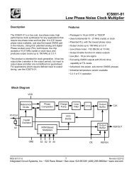
3.4 <strong>Force</strong>-Distance Curve<br />
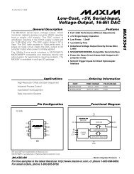
fo rc e c o n s ta n t k [N /m ]<br />
8 0<br />
7 0<br />
6 0<br />
5 0<br />
4 0<br />
3 0<br />
2 0<br />
2 6 0 2 8 0 3 0 0 3 2 0 3 4 0 3 6 0 3 8 0 4 0 0 4 2 0<br />
re s o n a n c e fre q u e n c y ω 0<br />
[k H z ]<br />
Figure 3.2: Determine the force constant<br />
read again the first three paragraphs of section 4.3.1.<br />
In order to set the sensitivity and to obtain metric deflection<br />
data, draw a trace parallel to the linear part<br />
of the force curve with the mouse in the force calibration<br />
plot. The experiments should be performed on<br />
two different objects: an old and a new mica sample<br />
where the influence of the water layer can be identified.<br />
Take one image of the force distance curve for<br />
each surface, choose the scaling parameters in a way<br />
that the interesting part of the curve is maximized.<br />
Images:<br />
• Screenshot of the resonance curve for the tip<br />
right before the measurement<br />
• <strong>Force</strong> Distance Curve for old mica surface<br />
• <strong>Force</strong> Distance Curve for cleaned mica surface<br />
Discuss the different parts of the curves and the<br />
difference between approaching and retracting. Additionally,<br />
the difference between the two samples<br />
should be identified and quantified by calculating the<br />
force that acts on the tip. Therefore determine the<br />
difference in deflection between the minimum and the<br />
constant part of the curve for the retraction. This<br />
difference has to be multiplied by the force constant<br />
that can be determined with the help of figure 3.2.<br />
13
3 Experiments and Evaluation<br />
Figure 3.3: Data sheet for calibration grid TGZ01-TGZ02<br />
14
4 Technical Support<br />
Table 4.1: Description of the menu buttons in the image<br />
mode.<br />
Approach surface automatically by step<br />
motor (max. 80 µm).<br />
Retract tip from surface (5 µm per turn);<br />
retract about 25 µm to change scan area<br />
and much more to change sample.<br />
Change to image mode (default).<br />
Table 4.2: Description of the menu buttons in the force<br />
mode.<br />
Retract tip from surface (5 µm per turn);<br />
retract about 25 µm to change scan area<br />
and much more to change sample.<br />
Capture image.<br />
Exit capture image.<br />
Single trace mode.<br />
Start scanning at bottom of scan area.<br />
Start scanning on top of scanning area.<br />
The tip is continuously lowered and raised<br />
by distance equal to the z scan size. This<br />
is the normal, default motion in the force<br />
mode.<br />
Approach and retract the surface once by<br />
a distance equal to the z scan size.<br />
<strong>Force</strong> curve mode.<br />
Search for resonance frequency mode.<br />
!<br />
Halts all tip movements.<br />
Change to image mode (default).<br />
Capture mode.<br />
Exit capture mode.<br />
This part will give a technical introduction in the<br />
use of the AFM type Multimode by Digital Instruments.<br />
It is meant to be a guide during the execution<br />
of the lab course, hence it is not necessary to read it<br />
in extension when preparing for the lab, but it should<br />
be read at the beginning of the lb course after the<br />
introduction of the tutor.<br />
Throughout the entire tutorial expressions which<br />
are related to the control software or the AFM itself<br />
will be given in sans serif font.<br />
4.1 Start-up<br />
1. Turn on the computer and scanner by the power<br />
button behind the screen.<br />
2. Open the program Nanoscope III 5.31r1 and turn<br />
the microscope button to start imaging, or the<br />
other button to open saved images.<br />
3. Under Microscope → Profile search for Tapping-<br />
AFM with file name afmprak2. All the parameters<br />
shown in this menu are described in the tables 4.1<br />
and 4.2.<br />
4. Place the sample on the magnetic sample holder<br />
above the piezo.<br />
5. Put the cantilever in the cantilever holder.<br />
6. Place the cantilever holder in the AFM head and<br />
fix it with adjustment I (as schematically shown<br />
in fig. 4.1).<br />
7. Move the sample to the area of interest with<br />
adjustments IIa and IIb using the optical microscope.<br />
(Steps 5, 6 and 8 up to 11 are only<br />
necessary when a new cantilever is used.)<br />
8. Locate the laser light on the cantilever tip. Before,<br />
verify that the mode switch on the multimode<br />
SPM’s base is switched to AFM & LFM.<br />
15
4 Technical Support<br />
Figure 4.1: Schematic image of the AFM head, a) front and b) rear view. For the description of the parts see text.<br />
Align the laser spot on the cantilever by the laser<br />
position adjustments IIIa (x-axis) and IIIb (yaxis).<br />
The maximised value for the SUM should<br />
be approximately 3.0–8.0 Volts.<br />
9. Adjust the photo-diode positioner (adjusters IVa<br />
and Ivb) to set the reflected laser beam in the<br />
middle of the diode. The values A-B and C-D<br />
should be close to zero.<br />
10. Put the mode switch on the multimode SPM’s<br />
base to TM AFM.<br />
11. Search for the resonant frequency by the 8th<br />
button in the upper screen (symbol “tuning<br />
fork”, see table 4.1). Auto tune will automatically<br />
search for this frequency and with back to<br />
image mode, this value will automatically set the<br />
value for drive frequency.<br />
12. Recheck all control panel parameters. The feedback<br />
gains and the scan rate are the most important<br />
parameters. Start with the integral gain<br />
set to 0.50 and the proportional gain set to about<br />
1.20. The scan rate should be set below 2 Hz.<br />
Use a scan size of 10 µm to get an overview.<br />
13. Focus with the optical microscope on the surface,<br />
e.g. an edge of the surface.<br />
14. Use the coarse adjustment screws and the step<br />
motor to bring tip and surface closer together.<br />
The AFM head has to be totally horizontal. If<br />
all goes well after re-engaging, a well-formed<br />
cantilever tip will begin to appear on the display<br />
monitor. Take care! If the sample is in focus,<br />
the tip has to be a little bit above the focus<br />
otherwise it will crash. Then use the first button<br />
in the upper screen (see table 4.1) to make the<br />
tip contacting the surface.<br />
15. After the tip contacts the sample, the AFM will<br />
automatically start scanning the sample.<br />
16. If the image doesn’t look like it should, you can<br />
try to adjust the scan controls described in the<br />
following section to improve the quality of the<br />
image.<br />
4.2 Parameters for Image Mode<br />
4.2.1 Scan Controls:<br />
Scan size: Size of the scan along one side of the<br />
square. If the scan is non-square (as determined<br />
by the aspect ratio parameter), the value<br />
entered is the longer of the two sides. Maximum/minimum<br />
value: 500 nm–10 µm.<br />
Aspect ratio: Determines whether the scan is to be<br />
square (aspect ratio 1:1), of non-square. Default<br />
value 1:1.<br />
X offset, Y offset: these controls allow adjustment<br />
of the lateral scanned area and the centre of<br />
the scanned area. These values can be chosen<br />
between 0 and maximal 10 µm, depending on the<br />
scan size (piezo deflection in x- and y-direction<br />
is max. 10 µm).<br />
Scan angle: Combines x-axis and y-axis drive voltages,<br />
causing the piezo to scan the sample at<br />
varying x-y angles. Value between 0 and 90<br />
degrees.<br />
Scan rate: The number of lines scanned per second<br />
in the fast scan (x-axis on display monitor) direction.<br />
In general, the scan rate must be decreased<br />
as the scan size is decreased. Scan rates if 1.5–2.5<br />
Hz should be used for larger scans on samples<br />
with tall features. High scan rates help to reduce<br />
16
4.2 Parameters for Image Mode<br />
drift, but they can only be used on very flat samples<br />
with small scan sizes. Maximum/minimum<br />
value: 0.1–5 Hz.<br />
Tip velocity: The scanned distance per second in<br />
the fast scan direction (changes as the scan rate<br />
changes).<br />
Samples/line: Number of imaged points per scanned<br />
line. Maximum/minimum value: 128–1024 (default<br />
value 512).<br />
Lines: number of scanned lines. This value is the<br />
same as samples/line for aspect ratio of 1:1. Maximum/minimum<br />
value: 128–1024; default value<br />
512.<br />
Number of samples: Sets the number of pixels displayed<br />
per line and the number of lines per<br />
scanned frame.<br />
Slow scan axis: Starts and stops the slow scan (yaxis<br />
on display monitor). This control is used to<br />
allow the user to check for lateral mechanical drift<br />
in the microscope or assist in tuning the feedback<br />
gains. Always set to enable unless checking for<br />
drift or tuning gains. Default value: enable.<br />
4.2.2 Feedback Controls<br />
SPM feedback: Sets the signal used as feedback input.<br />
Possible signals are Amplitude (default), TM<br />
deflection and Phase.<br />
Integral gain and proportional gain: Controls the<br />
response time of the feedback loop. The feedback<br />
loop tries to keep the output of the SPM equal<br />
to the setpoint reference chosen. It does this by<br />
moving the piezo in z to keep the SPM’s output<br />
on track with the setpoint reference. Piezoelectric<br />
transducers have a characteristic response<br />
time to the feedback voltage applied. The gains<br />
are simply values that magnify the difference<br />
read at the A/D converter. This causes the computer<br />
to think that the SPM output is further<br />
away from the setpoint reference than it really<br />
is. The computer essentially overcompensates<br />
for this by sending a larger voltage to the z<br />
piezo than it truly needed. This causes the piezo<br />
scanner to move faster in z. This is done to<br />
compensate for the mechanical hysteresis of the<br />
piezo element. The effect is smoothed out due<br />
to the fact that the piezo is adjusted up to four<br />
times the rate of the display rate. Optimise the<br />
integral gain and proportional gain so that the<br />
height image shows the sharpest contrast and<br />
there are minimal variations in the amplitude<br />
image (the error signal). It may be helpful to<br />
optimise the scan rate to get the sharpest image.<br />
Maximum/minimum value for integral gain:<br />
0.1–4 and for proportional gain: 0.1–10. Default<br />
values between 2 and 3.<br />
Amplitude setpoint: The setpoint defines the desired<br />
voltage for the feedback loop. The setpoint<br />
voltage is constantly compared to the present<br />
RMS amplitude voltage to calculate the desired<br />
change in the piezo position. When the SPM<br />
feedback is set to amplitude, the z piezo position<br />
changes to keep the amplitude voltage close to<br />
the setpoint; therefore, the vibration amplitude<br />
remains nearly constant. Changing the setpoint<br />
alters the response of the cantilever vibration<br />
and changes the amount of force applied to the<br />
sample. Maximum/minimum value: 1–8.<br />
Drive frequency: Defines the frequency at which the<br />
cantilever is oscillated. This frequency should<br />
be very close to the resonant frequency of the<br />
cantilever. These value is around 300 kHz for the<br />
cantilevers used.<br />
Drive amplitude: Defines the amplitude of the voltage<br />
applied to the piezo system that drives the<br />
cantilever vibration. It is possible to fracture<br />
the cantilever by using too high drive amplitude;<br />
therefore, it is safer to start with a small value<br />
and increase the value incrementally. If the amplitude<br />
calibration plot consist of a flat line all<br />
the way across, changing the value of this parameter<br />
should shift the level of the curve. If<br />
it does not, the tip is probably fully extended<br />
into the surface and the tip should be withdrawn<br />
before proceeding. Maximum/minimum value:<br />
10–60 mV, default 30 mV.<br />
4.2.3 Channel 1, 2 and 3<br />
Data type: Height data corresponds to the change<br />
in piezo height needed to keep the vibrational<br />
amplitude of the cantilever constant. Amplitude<br />
data describes the change in the amplitude<br />
directly. Deflection data comes from the differential<br />
signal off of the top and bottom photo-diode<br />
segments.<br />
Data scale: This parameter controls the vertical<br />
scale corresponding to the full height of the display<br />
and colour bar.<br />
Data centre: Offsets the centreline on the colour<br />
scale by the amount entered.<br />
Line direction: Selects the direction of the fast scan<br />
during data collection. Only one-way scanning<br />
is possible.<br />
Range of settings:<br />
17
4 Technical Support<br />
• Trace: Data is collected when the relative<br />
motion of the tip is left to right as viewed<br />
from the front of the microscope.<br />
• Retrace: Data is collected when the relative<br />
tip motion is right to left as viewed from<br />
the front of the microscope.<br />
Scan line: The scan line controls whether data from<br />
the Main of Interleave scan line is displayed and<br />
captured.<br />
Real-time plane fit: Applies a software leveling plane<br />
to each real-time image, thus removing up to firstorder<br />
tilt. Five types of plane-fit are available<br />
to each real-time image shown on the display<br />
monitor.<br />
Range of settings:<br />
• None: Only raw, unprocessed data is displayed.<br />
• Offset: Takes the z-axis average of each<br />
scan line, then subtracts it from every data<br />
point.<br />
• Line: Takes the slope and z-axis average of<br />
each scan line and subtracts it from each<br />
data point in that scan line. This is the<br />
default mode of operation, and should be<br />
used unless there is a specific reason to do<br />
otherwise.<br />
• AC: Takes the slope and z-axis average of<br />
each scan line across one-half of that line,<br />
then subtracts it from each data point in<br />
that scan line.<br />
• Frame: Level the real-time image based on<br />
a best-fit plane calculated from the most<br />
recent real-time frame performed with the<br />
same frame direction (up or down).<br />
• Captured: Level the real-time image based<br />
on a best fit plane calculated from a plane<br />
captured with the capture plane command<br />
in.<br />
Off line plane fit: Applies a software levelling plane<br />
to each off-line image for removing first-order<br />
tilt. Five types of plane-fit are available to each<br />
off-line image.<br />
Range of settings:<br />
• None: Only raw, unprocessed data is displayed.<br />
• Offset: Captured images have a DC z offset<br />
removed from them, but they are not fitted<br />
to a plane.<br />
• Full: A best-fit plane that is derived from<br />
the data file is subtracted from the captured<br />
image.<br />
High-pass filter: This filter parameter invokes a digital,<br />
two-pole, high-pass filter that removes low<br />
frequency effects, such as ripples caused by torsional<br />
forces on the cantilever when the scan<br />
reverses direction. It operates on the digital<br />
data stream regardless of scan direction. This<br />
parameter can be off or set from 0 through 9.<br />
Settings of 1 through 9, successively, lower the<br />
cut-off frequency of the filter applied to the data<br />
stream. It is important to realize that in removing<br />
low frequency information from the image,<br />
the high-pass filter distorts the height information<br />
in the image.<br />
Low-pass filter: This filter invokes a digital, onepole,<br />
low-pass filter to remove high-frequency<br />
noise from the Real Time data. The filter operates<br />
on the collected digital data regardless of<br />
the scan direction. Settings for this item range<br />
from off through 9. Off implies no low-pass filtering<br />
of the data, while settings of 1 through 9,<br />
successively, lower the cut-off frequency of the<br />
filter applied to the data stream.<br />
4.3 Parameters for <strong>Force</strong> Mode<br />
4.3.1 Main Control<br />
Ramp channel: Defines the variable to be plotted<br />
along the x-axis of the scope trace. Default Z.<br />
Ramp size: This parameter defines the total travel<br />
distance of the piezo. Use caution when working<br />
in the force mode. This mode can potentially<br />
damage the tip and/or surface by too high values<br />
for the ramp size.<br />
Z scan start: This parameter sets the offset of the<br />
piezo travel (i.e., its starting point). It sets the<br />
maximum voltage applied to the z electrodes of<br />
the piezo during the force plot operation. The<br />
triangular waveform is offset up and down in relation<br />
to the value of this parameter. Increasing<br />
the value of the z scan start parameter moves the<br />
sample closer to the tip by extending the piezo<br />
tube.<br />
Scan rate: sets the rate with which the z-piezo approach/retract<br />
the tip. Maximum/minimum<br />
value: 0.1–5 Hz.<br />
X offset and Y offset: controls the centre position<br />
of the scan in the x- and y- directions, respectively;<br />
same as in image mode. Range of settings:<br />
±220 V.<br />
Number of samples: Defines the number of data<br />
points captured during each extension/retraction<br />
18
4.4 Trouble Shooting<br />
cycle of the z-piezo. Maximum/minimum value:<br />
128–1024; default value 512.<br />
Average count: sets the number of scans taken to<br />
average the display of the force plot. May be set<br />
between 1 and 1024. Usually it is set to 1 unless<br />
the user needs to reduce noise.<br />
Spring constant: This parameter relates the cantilever<br />
deflection signal to the z travel of the<br />
piezo. It equals the slope of the deflection versus<br />
z when the tip is in contact with the sample. For<br />
a proper force curve, the line has a negative slope<br />
with typical values of 10–50 mV/nm; however,<br />
by convention, values are shown as positive in<br />
the menu.<br />
Display mode: The portion of a tip’s vertical motion<br />
to be plotted on the force graph.<br />
Range of settings:<br />
• Extend: Plots only the extension portion of<br />
the tip’s vertical travel.<br />
• Retract: Plots only the retraction portion<br />
of the tip’s vertical travel.<br />
• Both: Plots both the extension and retraction<br />
portion of the tip’s vertical travel.<br />
Units: This item selects the units of the parameters,<br />
either metric lengths or volts.<br />
X rotate: allows the user to move the tip laterally,<br />
in the x-direction, during indentation. This is<br />
useful since the cantilever is at an angle relative<br />
to the surface. One purpose of X rotate is to<br />
prevent the cantilever from ploughing the surface<br />
laterally, typically along the x-direction, while it<br />
indents in the sample surface in the z-direction.<br />
Ploughing can occur due to cantilever bending<br />
during indentation of due to x-movement caused<br />
by coupling of the z and x axes of the piezo scanner.<br />
When indenting in the z-direction, the X rotate<br />
parameter allows the user to add movement<br />
in the x-direction. X rotate causes movement of<br />
the scanner opposite to the direction in which<br />
the cantilever points. Without X rotate control.<br />
The tip may be prone to pitch forward during<br />
indentation. It can be varied in a range of 0–90<br />
degrees. Normally, it is set to about 22 degrees.<br />
Amplitude setpoint: Same as in image mode.<br />
4.3.2 Channel 1, 2 and 3<br />
Data type/data scale/data centre: Same as in image<br />
mode.<br />
Amplitude sens.: This item relates the vibrational<br />
amplitude of the cantilever to the z travel of<br />
the piezo. It is calculated by measuring the<br />
slope of the RMS amplitude versus the z voltage<br />
when the tip is in contact with the sample. The<br />
NanoScope system automatically calculates and<br />
enters the value from the graph after the operator<br />
uses the mouse to fit a line to the graph. This<br />
item must be properly calculated and entered<br />
before reliable deflection data in nanometers can<br />
be displayed. For a proper force curve, the line<br />
has a negative slope with typical values of 10–<br />
50 mV/nm; however, by convention, values are<br />
shown as positive in the menu.<br />
4.4 Trouble Shooting<br />
It happens rather often that one thinks to have<br />
checked all control panel parameters correctly but<br />
does not get an image. Here a list of the most common<br />
errors.<br />
• Right input channel (see monitor). Height signal<br />
for constant height and deflection signal for<br />
constant deflection mode.<br />
• Correct gains for proportional gain and integral<br />
gain. These parameters have to be between 0.1<br />
and 5, depending on the softness/hardness of the<br />
sample. Start with the integral gain set to 0.50<br />
and the proportional gain set to about 1.20.<br />
• Is the height scale justified correctly for the different<br />
channels?<br />
• What is the size of the scan area? The scan size<br />
can be varied between 100 nm and 10 µm. Use<br />
a scan size of 10 µm to get an overview.<br />
• Is the piezo in its limit between + and −220 V?<br />
This can be checked by the green/red setpoint<br />
line in the approach/retract bar. This green/red<br />
setpoint line should not be on the left or on the<br />
right site of the bar. This can be changed by the<br />
amplitude setpoint parameter.<br />
• Does the force used to image the probe destroy<br />
the probe? Play around with the amplitude setpoint<br />
parameter and the drive amplitude parameter.<br />
The slope of the force curve shows the<br />
sensitivity of the TappingMode measurement. In<br />
general, higher sensitivities will give better image<br />
quality. The View → <strong>Force</strong> Mode → plot<br />
command plots the cantilever amplitude versus<br />
the scanner position (=force curve). The curve<br />
should show a mostly flat region where the cantilever<br />
has not yet reached the surface and the<br />
19
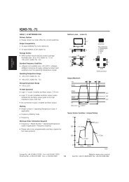
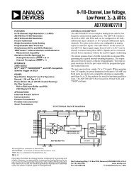
4 Technical Support<br />
Figure 4.2: Artifacts can occur due to a defective tip. Left: a multiple tip occurs as a pattern; middle: repeating<br />
patterns due to several tip areas scanning at the same time; right: silverfish structures due to high setpoint<br />
sloped region where the amplitude is being reduced<br />
by the tapping interaction. To protect<br />
the tip and sample, take care that the cantilever<br />
amplitude is never reduced to zero. Adjust the<br />
setpoint until the green setpoint line on the graph<br />
is just barely below the flat region of the force<br />
curve. This is the setpoint that applies the lowest<br />
force on the sample.<br />
4.5 Poor Image Quality<br />
Contaminated tip<br />
Some types of samples may adhere to the cantilever<br />
and tip (e.g. certain proteins). This will reduce resolution<br />
giving fuzzy images. If the tip contamination<br />
is suspected to be a problem, it will be necessary to<br />
protect the tip against contamination.<br />
Dull tip<br />
AFM cantilever tips can become dull during use and<br />
some unused tips may be defective. If imaging resolution<br />
is poor, try changing to a new cantilever.<br />
has to be changed.<br />
Too low setpoint<br />
Some structure shows up that does not exist (e.g.<br />
circles). Change the amplitude setpoint to a better<br />
value.<br />
Too high setpoint<br />
If silverfish structures appear (see figure 4.2 right),<br />
the adjustment of the integral and proportional gain<br />
can help, but if the setpoint is not adjusted correctly,<br />
increasing the gain will worse the noise of the image.<br />
Too high drive frequency<br />
The image surface looks destroyed; e.g. holes appear.<br />
These holes are artifacts and disappear when the<br />
drive frequency is lowered.<br />
Other error sources<br />
• Scanner beeps loud: decrease immediately the<br />
gains; the scanner is over-driven.<br />
Multiple tip<br />
AFM cantilevers can have multiple protrusions at the<br />
apex of the tip which result in image artifacts. In<br />
this case, features on the surface will appear two or<br />
more times in the image, usually separated by several<br />
nanometers (see figure 4.2 left). If this occurs and<br />
this effect doesn’t disappear after some time, change<br />
of clean the AFM tip.<br />
Repeating pattern<br />
If a repeating pattern appears, more tip areas scan<br />
simultaneous (see figure 4.2 middle). Such a cantilever<br />
• The image seems only noise: Adjust amplitude<br />
setpoint.<br />
• Strong drift of signal: approach the tip from the<br />
surface with the 2nd button in the upper screen<br />
and retract again.<br />
• During retraction of the tip, the scanner shows<br />
immediately contact with the surface, the image<br />
shows only noise: check the setpoint. Put the<br />
setpoint to zero and approach the surface again.<br />
20
Bibliography<br />
[1] G. Binnig, H. Rohrer, Ch. Gerber, and E. Weibel.<br />
Tunneling through a controllable vacuum gap.<br />
Appl. Phys. Lett., 40(2):178–180, 1982.<br />
[2] G. Binnig, H. Rohrer, Ch. Gerber, and E. Weibel.<br />
Surface studies by scanning tunneling microscopy.<br />
Phys. Rev. Lett., 49(1):57–61, 1982.<br />
[3] H. Lüth. Solid Surfaces, Interfaces and Thin<br />
Films. Springer, 4. edition, 2001.<br />
[4] M. Henzler and W. Göpel. Oberflächenphysik des<br />
Festkörpers. B. G. Teubner, Stuttgart, 1991.<br />
[5] G. Binnig, C. F. Quate, and Ch. Gerber. <strong>Atomic</strong><br />
force microscope. Phys. Rev. Lett., 56(9):930–933,<br />
Mar 1986.<br />
[6] R. Waser, editor. Nanoelectronics and Information<br />
Technology. Wiley-VCH, 2003.<br />
[7] K. Szot, W. Speier, U. Breuer, R. Meyer, J. Szade,<br />
and R. Waser. Formation of micro-crystals on the<br />
(1 0 0) surface of SrTiO 3 at elevated temperatures.<br />
Surf. Sci., 460:112–128, 2000.<br />
[8] S. Lee and W.M. Sigmund. AFM study of repulsive<br />
van der waals forces between teflon af<br />
thin film and silica or alumina. Colloids and Surfaces<br />
A: Physicochemical and Engineering Aspects,<br />
204:43–50, 2002.<br />
21