Development of a Novel Mass Spectrometric ... - Jacobs University
Development of a Novel Mass Spectrometric ... - Jacobs University Development of a Novel Mass Spectrometric ... - Jacobs University
Results and Discussion As far as comparing dirty oil to unused one is concerned, Kendrick plot allowed giving an insightful idea about what happens to the composition of oil engine upon mileage. Figure 3-87 shows a Kendrick plot of general standard car oil from Calpam Company overlapped to a contaminated-through-usage oil from an unknown car. Assuming that this Calpam oil or a similar one has been used in a new car and changed after a certain interval of time to give the contaminated one, the plot shows a depletion of the oil structural composition. It seems that the components have been degraded by observing the shift of KMD value of the contaminated through usage oil components compared with those of Calpam oil. As well decomposition of the oil is significant in plot. A large number of decomposed compounds appear in low mass range of m/z 100-250. These compounds are not found within the Calpam sample. To this end, this approach can be employed to understand compositional evolution of car motor oils after they are used. Understanding such changes in composition can guide car oil companies in developing better car oil that can serve for prolonged period before service is needed. KMD 1.1 Calpam Motor Oil Dirty Motor Oil 1 0.9 0.8 0.7 0.6 0.5 0.4 0 100 200 300 400 500 600 700 800 NKM Figure 3-87 Kendrick plot overlap of Calpam motor oil and contaminated through usage motor oil 111
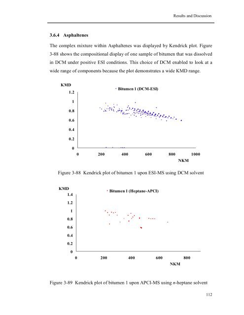
Results and Discussion 3.6.4 Asphaltenes The complex mixture within Asphaltenes was displayed by Kendrick plot. Figure 3-88 shows the compositional display of one sample of bitumen that was dissolved in DCM under positive ESI conditions. This choice of DCM enabled to look at a wide range of components because the plot demonstrates a wide KMD range. KMD 1.2 Bitumen 1 (DCM-ESI) 1 0.8 0.6 0.4 0.2 0 0 200 400 600 800 1000 NKM Figure 3-88 Kendrick plot of bitumen 1 upon ESI-MS using DCM solvent KMD 1.4 Bitumen 1 (Heptane-APCI) 1.2 1 0.8 0.6 0.4 0.2 0 0 200 400 600 800 NKM Figure 3-89 Kendrick plot of bitumen 1 upon APCI-MS using n-heptane solvent 112
- Page 77 and 78: Results and Discussion 519.5863 519
- Page 79 and 80: Results and Discussion Higher mass
- Page 81 and 82: Results and Discussion Intens. [%]
- Page 83 and 84: Results and Discussion Intens. [%]
- Page 85 and 86: Results and Discussion Intens. [%]
- Page 87 and 88: Results and Discussion isolated fro
- Page 89 and 90: Results and Discussion Intens. [%]
- Page 91 and 92: Results and Discussion Intens. [%]
- Page 93 and 94: Results and Discussion 3.4.5 Tandem
- Page 95 and 96: Results and Discussion Intens. [%]
- Page 97 and 98: Results and Discussion injected int
- Page 99 and 100: Results and Discussion Intens. [%]
- Page 101 and 102: Results and Discussion 3.4.8 Quanti
- Page 103 and 104: Results and Discussion Int. x 10000
- Page 105 and 106: Results and Discussion Table 3.6 Qu
- Page 107 and 108: Results and Discussion assessment o
- Page 109 and 110: Results and Discussion hydrocarbons
- Page 111 and 112: Results and Discussion Intens. [%]
- Page 113 and 114: Results and Discussion Intens. [%]
- Page 115 and 116: Results and Discussion Intens. [%]
- Page 117 and 118: Results and Discussion of n-alkanes
- Page 119 and 120: Results and Discussion flow (in I2)
- Page 121 and 122: Results and Discussion Other intere
- Page 123 and 124: Results and Discussion Figure 3-80
- Page 125 and 126: Results and Discussion KMD 2.4 2.2
- Page 127: Results and Discussion KMD 1.1 1 Le
- Page 131 and 132: Conclusions In conclusion we could
- Page 133 and 134: References References 1. Fay, R. M.
- Page 135 and 136: References 23. Colavecchia, M. V.,
- Page 137 and 138: References 47. Dzidic, I., Petersen
- Page 139 and 140: References Hydroconversion Processe
- Page 141 and 142: References 91. Golovlev, V. V., All
- Page 143 and 144: Appendix Light shredder waste Meas.
- Page 145 and 146: 419.4592 C 30 H 59 419.4611 4.6 421
- Page 147 and 148: Liqui Moly car motor oil Meas. m/z
- Page 149 and 150: 345.3511 C 25 H 45 345.3516 1.5 349
Results and Discussion<br />
3.6.4 Asphaltenes<br />
The complex mixture within Asphaltenes was displayed by Kendrick plot. Figure<br />
3-88 shows the compositional display <strong>of</strong> one sample <strong>of</strong> bitumen that was dissolved<br />
in DCM under positive ESI conditions. This choice <strong>of</strong> DCM enabled to look at a<br />
wide range <strong>of</strong> components because the plot demonstrates a wide KMD range.<br />
KMD<br />
1.2<br />
Bitumen 1 (DCM-ESI)<br />
1<br />
0.8<br />
0.6<br />
0.4<br />
0.2<br />
0<br />
0 200 400 600 800 1000<br />
NKM<br />
Figure 3-88 Kendrick plot <strong>of</strong> bitumen 1 upon ESI-MS using DCM solvent<br />
KMD<br />
1.4<br />
Bitumen 1 (Heptane-APCI)<br />
1.2<br />
1<br />
0.8<br />
0.6<br />
0.4<br />
0.2<br />
0<br />
0 200 400 600 800<br />
NKM<br />
Figure 3-89 Kendrick plot <strong>of</strong> bitumen 1 upon APCI-MS using n-heptane solvent<br />
112


