Itinerant Spin Dynamics in Structures of ... - Jacobs University

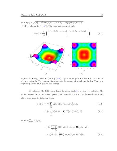
Chapter 5: Spin Hall Effect 87
with ∆(k) = √ (α 2 2 + ˜α2 1 )(sin(k x) 2 +sin(k y ) 2 )−4α 2˜α 1 sin(k x )sin(k y )
(E − (k) is plotted in Fig.5.1). The eigenvectors are given by
⎛
|+/−〉 = √ 1 ⎝
2
∓({˜α 1 sin(k x)−α 2 sin(k y)}+i{˜α 1 sin(k y)−α 2 sin(k x)})
∆
1
⎞
⎠ (5.11)
(a)
(b)
Figure 5.1: Energy band E − (k), Eq.(5.10) is plotted for pure Rashba SOC as function
of wave vector k. The contour lines indicate the energy at which one finds a Van Hove
singularity in the DOS (below half-filling).
To calculate the SHE using Kubo formula, Eq.(5.5), we have to calculate the
matrix elements of spin current operator and velocity operator. In the site basis of our
lattice they have the following form:
〈n|v|m〉 = 〈0| ∑ ij
αβ
= 〈0| ∑ ij
αβ
ψn(i,α)c ∗ iα vψ m (j,β)c † jβ
|0〉, (5.12)
ψn(i,α)c ∗ 1
iα
i [r,H]ψ m(j,β)c † jβ
|0〉, (5.13)
with r = ∑ kσ r kc † kσ c kσ
= 1 i 〈0|∑ kγ
∑
ψn ∗ (i,α)c iα[r k c † kγ c kγ]Hc † jβ ψ m(j,β)
ij
αβ
−ψ ∗ n(i,α)c iα
1
i H[c† kγ c kγr k ]c † jβ ψ m(j,β)|0〉, (5.14)