Itinerant Spin Dynamics in Structures of ... - Jacobs University

32 Chapter 3: WL/WAL Crossover and Spin Relaxation in Confined Systems
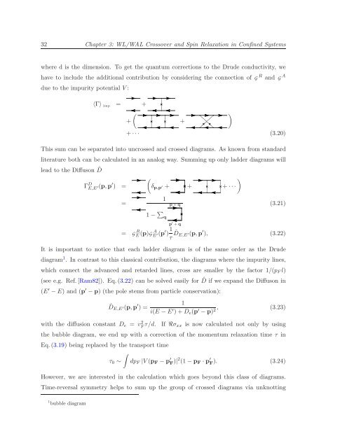
where d is the dimension. To get the quantum corrections to the Drude conductivity, we
have to include the additional contribution by considering the connection ofG R andG A
due to the impurity potential V:
〈Γ〉 imp = +
(
+
+
)
+··· (3.20)
This sum can be separated into uncrossed and crossed diagrams. As known from standard
literature both can be calculated in an analog way. Summing up only ladder diagrams will
lead to the Diffuson ˆD
Γ D E,E ′(p,p′ ) =
(
)
δ p,p ′ + + +···
=
1
p+q
(3.21)
1− ∑ q
p ′ +q
= G R E(p)G A E ′(p′ ) 1 τ ˆD E,E ′(p,p ′ ), (3.22)
It is important to notice that each ladder diagram is of the same order as the Drude
diagram 1 . In contrast to this classical contribution, the diagrams where the impurity lines,
which connect the advanced and retarded lines, cross are smaller by the factor 1/(p F l)
(see e.g. Ref.[Ram82]). Eq.(3.22) can be solved easily for ˆD if we expand the Diffuson in
(E ′ −E) and (p ′ −p) (the pole stems from particle conservation):
ˆD E,E ′(p,p ′ ) =
1
i(E −E ′ )+D e (p ′ −p) 2, (3.23)
with the diffusion constant D e = v 2 F τ/d. If Rσ xx is now calculated not only by using
the bubble diagram, we end up with a correction of the momentum relaxation time τ in
Eq.(3.19) being replaced by the transport time
∫
τ 0 ∼ dp F |V(p F −p ′ F )|2 (1−p F ·p ′ F ). (3.24)
However, we are interested in the calculation which goes beyond this class of diagrams.
Time-reversal symmetry helps to sum up the group of crossed diagrams via unknotting
1 bubble diagram