Itinerant Spin Dynamics in Structures of ... - Jacobs University

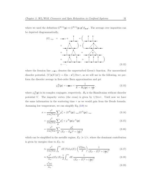
Chapter 3: WL/WAL Crossover and Spin Relaxation in Confined Systems 31
where we used the definition G R/A (p) ≡ G R/A (p,p ′ )δ p,p ′. The average over impurities can
be depicted diagrammatically,
(
〈G〉 imp = + +
) (
+ +
+ +
+ +
)
where the fermion line
+··· , (3.12)
denotes the unperturbed Green’s function. For uncorrelated
disorder potential, 〈V(x)V(x ′ )〉 = δ(x−x ′ )/2πντ, as we will use in the following, we perform
the disorder average in first-order Born approximation and get
G R E(p) = =
1
E −H 0 (p)+i 1 , (3.13)
2τ
whereG A E (p) is its complex conjugate, respectively. H 0 is the Hamiltonian without disorder
potential V. The impurity vertex (the cross) is given by 1/2πντ. Until now we have
the same information in the scattering time τ as we would gain from the Drude formula.
Assuming low temperature, we can simplify Eq.(3.9) to
e 2 ∑
σ =
πm 2 e Vol p 2 x ×〈G R (p)〉 imp 〈G A (p)〉 imp (3.14)
p
e 2 ∑
=
πm 2 e Vol p 2 x ×G R (p)G A (p) (3.15)
=
p
e 2 ∑ p 2 x
πm 2 e Vol p (E F −E p ) 2 + ( )
1 2
(3.16)
2τ
which can be simplified in the metallic regime, E F ≫ 1/τ, where the dominant contribution
is given by energies close to E F , to
e 2 ∫ ∞
( ) E2me
≈
πm 2 dE(Volρ(E))
eVol
d
≈ 2 e2
m e
ρ(E F )E F
1
d
0
∫ ∞
∞
dE
1
(E F −E) 2 + ( 1
2τ
1
(E F −E) 2 + ( 1
2τ
) 2
(3.17)
) 2
(3.18)
= e2 nτ
m e
, (3.19)