Itinerant Spin Dynamics in Structures of ... - Jacobs University
Itinerant Spin Dynamics in Structures of ... - Jacobs University Itinerant Spin Dynamics in Structures of ... - Jacobs University
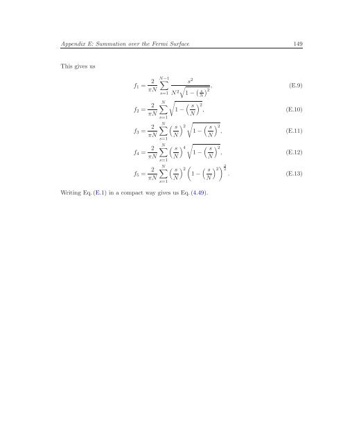
Appendix E Summation over the Fermi Surface The Cooperon Hamiltonian in the 2D case is given by H c = τv 2 {〈cos 2 (ϕ)〉(Q+2m e a.S) 2 x +〈sin 2 (ϕ)〉(Q+2m e a.S) 2 y +4m 2 e γ Dv 2 〈cos 2 (ϕ)sin 2 (ϕ)〉(Q+2m e a.S) x .S x −4m 2 eγ D v 2 〈sin 2 (ϕ)cos 2 (ϕ)〉(Q+2m e a.S) y .S y +(2m 3 e γ Dv 2 ) 2 (〈cos 2 (ϕ)sin 4 (ϕ)〉Sx 2 +〈sin 2 (ϕ)cos 4 (ϕ)〉S 2 y)}, (E.1) with wave vector Q. We set m e ≡ 1, f 1 := 〈sin 2 (ϕ)〉, f 2 := 〈cos 2 (ϕ)〉, f 3 := 〈sin 2 (ϕ)cos 2 (ϕ)〉, f 4 := 〈sin 4 (ϕ)cos 2 (ϕ)〉, f 5 := 〈sin 2 (ϕ)cos 4 (ϕ)〉. (E.2) (E.3) (E.4) (E.5) (E.6) (E.7) Using the Matsubara trick we write ∫ 2π 0 dϕ 2π = 2 πN N∑ 1 √ 1− ( ) . (E.8) s 2 N s=1 148
Appendix E: Summation over the Fermi Surface 149 This gives us f 1 = 2 N−1 ∑ πN s=1 f 2 = 2 πN f 3 = 2 πN f 4 = 2 πN f 5 = 2 πN s 2 N √1− ( ) , (E.9) 2 s 2 N √ N∑ ( s ) 2, 1− (E.10) N s=1 N∑ ( s ) √ 2 ( s ) 2, 1− (E.11) N N s=1 N∑ ( s ) √ 4 ( s ) 2, 1− (E.12) N N s=1 N∑ s=1 Writing Eq.(E.1) in a compact way gives us Eq.(4.49). ( ( )3 s 2 ( s 2 2 1− . (E.13) N) N)
- Page 107 and 108: Chapter 5: Spin Hall Effect 97 oper
- Page 109 and 110: Chapter 5: Spin Hall Effect 99 the
- Page 111 and 112: Chapter 5: Spin Hall Effect 101 str
- Page 113 and 114: Chapter 5: Spin Hall Effect 103 Com
- Page 115 and 116: Chapter 5: Spin Hall Effect 105 Fin
- Page 117 and 118: Chapter 6: Critical Discussion and
- Page 119 and 120: Chapter 6: Critical Discussion and
- Page 121 and 122: List of Figures 111 3.3 Exemplifica
- Page 123 and 124: List of Figures 113 4.2 The spin de
- Page 125 and 126: List of Tables 3.1 Singlet and trip
- Page 127 and 128: Bibliography 117 [BB04] [BBF + 88]
- Page 129 and 130: Bibliography 119 [DP71b] [DP71c] [D
- Page 131 and 132: Bibliography 121 [HSM + 06] [HSM +
- Page 133 and 134: Bibliography 123 [MACR06] T. Mickli
- Page 135 and 136: Bibliography 125 [PMT88] [PP95] [PT
- Page 137 and 138: Bibliography 127 [Tor56] H. C. Torr
- Page 139 and 140: Appendix A SOC Strength in the Expe
- Page 141 and 142: Appendix A: SOC Strength in the Exp
- Page 143 and 144: Appendix B: Linear Response 133 in
- Page 145 and 146: Appendix B: Linear Response 135 Pro
- Page 147 and 148: Appendix C Cooperon and Spin Relaxa
- Page 149 and 150: Appendix C: Cooperon and Spin Relax
- Page 151 and 152: Appendix C: Cooperon and Spin Relax
- Page 153 and 154: Appendix C: Cooperon and Spin Relax
- Page 155 and 156: Appendix C: Cooperon and Spin Relax
- Page 157: Appendix D: Hamiltonian in [110] gr
- Page 161: Appendix F: KPM 151 integer running
Appendix E: Summation over the Fermi Surface 149<br />
This gives us<br />
f 1 = 2 N−1<br />
∑<br />
πN<br />
s=1<br />
f 2 = 2<br />
πN<br />
f 3 = 2<br />
πN<br />
f 4 = 2<br />
πN<br />
f 5 = 2<br />
πN<br />
s 2<br />
N<br />
√1− ( ) , (E.9)<br />
2 s 2<br />
N<br />
√ N∑ ( s<br />
) 2,<br />
1−<br />
(E.10)<br />
N<br />
s=1<br />
N∑ ( s<br />
)<br />
√<br />
2 ( s<br />
) 2,<br />
1−<br />
(E.11)<br />
N N<br />
s=1<br />
N∑ ( s<br />
)<br />
√<br />
4 ( s<br />
) 2,<br />
1−<br />
(E.12)<br />
N N<br />
s=1<br />
N∑<br />
s=1<br />
Writ<strong>in</strong>g Eq.(E.1) <strong>in</strong> a compact way gives us Eq.(4.49).<br />
( ( )3<br />
s 2 ( s 2 2<br />
1− . (E.13)<br />
N)<br />
N)


