Itinerant Spin Dynamics in Structures of ... - Jacobs University
Itinerant Spin Dynamics in Structures of ... - Jacobs University Itinerant Spin Dynamics in Structures of ... - Jacobs University
142 Appendix C: Cooperon and Spin Relaxation duetodephasingc 1 = 1/D e Q 2 SO τ ϕ andelasticscatteringc 2 = 1/D e Q 2 SO τ determinewhether we have a positive or negative correction. Integrating over all possible wave vectors K = k/Q SO in the case without boundaries yields ∆σ = − 2e2 2π ∫ √ 1 c2 ( (2π) 2 dK(2πK) 0 1 + E T+ (Q SO K)/Q 2 + SO +c 1 1 1 − E S (Q SO K)/Q 2 + SO +c 1 E T0 (Q SO K)/Q 2 SO +c 1 ) 1 E T− (Q SO K)/Q 2 SO +c 1 (C.38) = − 2e2 2π ⎧ ⎪⎨ arctan + ⎪⎩ ⎧ ⎪⎨ arctan + ⎪⎩ (− 1 2 ln ( 1+ c 2 ( ( c 1 ) 5 √ 1 4 7 16 +c 1 3 √ 1 4 7 16 +c 1 ) √ ) √ + 1 2 ln ( 1+ c 2 −arctan 7 16 +c 1 +arctan 7 16 +c 1 1+c 1 ) ( √ 1 16 +c 2+1 √ 7 16 +c 1 ( √ 1 16 +c 2−1 √ 7 16 +c 1 ) ) ⎛ − 1 2 ln ⎝ ⎛ − 1 2 ln ⎝ 2+c 1 √ 3 2 +c 1 +c 2 +2 1+c 1 √ 3 2 +c 1 +c 2 −2 1 16 +c 2 1 16 +c 2 ⎫ ⎞ ⎪⎬ ⎠ ⎪⎭ ⎫ ⎞ ⎪⎬ ⎠ ). (C.39) ⎪⎭ As an example, we choose parameters which have been used in the case of boundaries, 1/D e Q 2 τ SO ϕ = 0.08,1/D e Q 2 τ = 4: SO ∆σ/(2e2 /2π) = −0.29. The exact calculation of wide wires (Q SO W > 1) approaches this limit as can be seen in Fig.3.11. The weak localization correction in 2D as function of these C.5 Exact Diagonalization We write the inverse Cooperon propagator, the Hamiltonian ˜H c , in the representation of the longitudinal momentum Q x , the quantized transverse momentum with quantum numbern ∈ N, and in the representation of singlet and triplet states with quantum numbers S,m, where we note that ˜H c is diagonal in Q x , 〈Q x ,n,S,m | ˜H c | Q x ,n ′ ,S ′ ,m ′ 〉. (C.40)
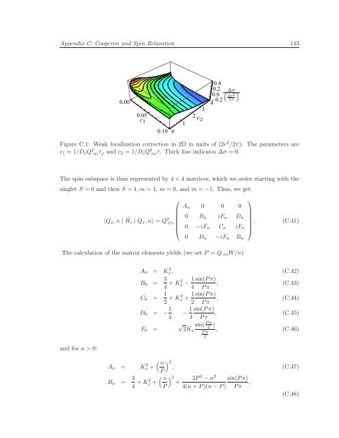
Appendix C: Cooperon and Spin Relaxation 143 0.00 0.05 c 1 c 2 0.10 0 1 2 3 0.4 0.2 4 0.2 0.0 “ ∆σ ” 2e 2 2π Figure C.1: Weak localization correction in 2D in units of (2e 2 /2π). The parameters are c 1 = 1/D e Q 2 SOτ ϕ and c 2 = 1/D e Q 2 SOτ. Thick line indicates ∆σ = 0. The spin subspace is thus represented by 4×4 matrices, which we order starting with the singlet S = 0 and then S = 1,m = 1, m = 0, and m = −1. Thus, we get ⎛ ⎞ A n 0 0 0 〈Q x ,n | ˜H c | Q x ,n〉 = Q 2 0 B n iF n D n SO . (C.41) ⎜ ⎝ 0 −iF n C n iF n ⎟ ⎠ 0 D n −iF n B n The calculation of the matrix elements yields (we set P = Q SO W/π) and for n > 0: A 0 = Kx 2 , (C.42) B 0 = 3 4 +K2 x − 1 sin(Pπ) , 4 Pπ (C.43) C 0 = 1 2 +K2 x + 1 sin(Pπ) , 2 Pπ (C.44) D 0 = − 1 − 1 sin(Pπ) , 4 4 Pπ (C.45) F 0 = √ sin( Pπ 2Kx , (C.46) 2 ) Pπ 2 ( n ) 2, A n = Kx 2 + (C.47) P B n = 3 4 +K2 x + ( n P ) 2 + 2P 2 −n 2 4(n+P)(n−P) sin(Pπ) , Pπ (C.48)
- Page 101 and 102: Chapter 5: Spin Hall Effect 91 as s
- Page 103 and 104: Chapter 5: Spin Hall Effect 93 V⩵
- Page 105 and 106: Chapter 5: Spin Hall Effect 95 0.4
- Page 107 and 108: Chapter 5: Spin Hall Effect 97 oper
- Page 109 and 110: Chapter 5: Spin Hall Effect 99 the
- Page 111 and 112: Chapter 5: Spin Hall Effect 101 str
- Page 113 and 114: Chapter 5: Spin Hall Effect 103 Com
- Page 115 and 116: Chapter 5: Spin Hall Effect 105 Fin
- Page 117 and 118: Chapter 6: Critical Discussion and
- Page 119 and 120: Chapter 6: Critical Discussion and
- Page 121 and 122: List of Figures 111 3.3 Exemplifica
- Page 123 and 124: List of Figures 113 4.2 The spin de
- Page 125 and 126: List of Tables 3.1 Singlet and trip
- Page 127 and 128: Bibliography 117 [BB04] [BBF + 88]
- Page 129 and 130: Bibliography 119 [DP71b] [DP71c] [D
- Page 131 and 132: Bibliography 121 [HSM + 06] [HSM +
- Page 133 and 134: Bibliography 123 [MACR06] T. Mickli
- Page 135 and 136: Bibliography 125 [PMT88] [PP95] [PT
- Page 137 and 138: Bibliography 127 [Tor56] H. C. Torr
- Page 139 and 140: Appendix A SOC Strength in the Expe
- Page 141 and 142: Appendix A: SOC Strength in the Exp
- Page 143 and 144: Appendix B: Linear Response 133 in
- Page 145 and 146: Appendix B: Linear Response 135 Pro
- Page 147 and 148: Appendix C Cooperon and Spin Relaxa
- Page 149 and 150: Appendix C: Cooperon and Spin Relax
- Page 151: Appendix C: Cooperon and Spin Relax
- Page 155 and 156: Appendix C: Cooperon and Spin Relax
- Page 157 and 158: Appendix D: Hamiltonian in [110] gr
- Page 159 and 160: Appendix E: Summation over the Ferm
- Page 161: Appendix F: KPM 151 integer running
Appendix C: Cooperon and <strong>Sp<strong>in</strong></strong> Relaxation 143<br />
0.00<br />
0.05<br />
c 1<br />
c 2<br />
0.10 0<br />
1<br />
2<br />
3<br />
0.4<br />
0.2<br />
4 0.2<br />
0.0<br />
“ ∆σ ”<br />
2e 2<br />
2π<br />
Figure C.1: Weak localization correction <strong>in</strong> 2D <strong>in</strong> units <strong>of</strong> (2e 2 /2π). The parameters are<br />
c 1 = 1/D e Q 2 SOτ ϕ and c 2 = 1/D e Q 2 SOτ. Thick l<strong>in</strong>e <strong>in</strong>dicates ∆σ = 0.<br />
The sp<strong>in</strong> subspace is thus represented by 4×4 matrices, which we order start<strong>in</strong>g with the<br />
s<strong>in</strong>glet S = 0 and then S = 1,m = 1, m = 0, and m = −1. Thus, we get<br />
⎛<br />
⎞<br />
A n 0 0 0<br />
〈Q x ,n | ˜H c | Q x ,n〉 = Q 2 0 B n iF n D n<br />
SO<br />
. (C.41)<br />
⎜<br />
⎝ 0 −iF n C n iF n<br />
⎟<br />
⎠<br />
0 D n −iF n B n<br />
The calculation <strong>of</strong> the matrix elements yields (we set P = Q SO W/π)<br />
and for n > 0:<br />
A 0 = Kx 2 ,<br />
(C.42)<br />
B 0 = 3 4 +K2 x − 1 s<strong>in</strong>(Pπ)<br />
,<br />
4 Pπ<br />
(C.43)<br />
C 0 = 1 2 +K2 x + 1 s<strong>in</strong>(Pπ)<br />
,<br />
2 Pπ<br />
(C.44)<br />
D 0 = − 1 − 1 s<strong>in</strong>(Pπ)<br />
,<br />
4 4 Pπ<br />
(C.45)<br />
F 0 =<br />
√ s<strong>in</strong>( Pπ<br />
2Kx , (C.46)<br />
2 )<br />
Pπ<br />
2<br />
( n<br />
) 2,<br />
A n = Kx 2 +<br />
(C.47)<br />
P<br />
B n = 3 4 +K2 x + ( n<br />
P<br />
) 2<br />
+<br />
2P 2 −n 2<br />
4(n+P)(n−P)<br />
s<strong>in</strong>(Pπ)<br />
,<br />
Pπ<br />
(C.48)


