Spatially-averaged model for plasma etch processes ... - IWR

Spatially-averaged model for plasma etch processes: Comparison
of different approaches to electron kinetics
P. Ahlrichs, U. Riedel, a) and J. Warnatz
Interdisziplinäres Zentrum für Wissenschaftliches Rechnen, Universität Heidelberg, Im Neuenheimer Feld
368, D-69120 Heidelberg, Germany
Received 30 September 1997; accepted 8 December 1997
A well stirred reactor model determines spatially averaged species composition in a plasma etch
reactor by solving conservation equations for species, mass, and electron energy distribution
function EEDF. The reactor is characterized by a chamber volume, surface area, mass flow,
pressure, power deposition, and composition of the feed gas. The well stirred reactor model is
increasingly common in the literature due to its low requirement of computer resources for detailed
chemical kinetics calculations. In such plasma etch models, assumptions on the EEDF, which are
needed to determine reaction rate coefficients for electron impact reactions, are crucial for a
prediction of steady state conditions. In this article we focus on a comparison for three different
levels of sophistication with regard to the electron energy distribution function: obtaining the EEDF
from a fully coupled solution of species equations and the Boltzmann equation, pre-computing and
tabulating the EEDF for typical reactor conditions, and assuming a Maxwellian EEDF. The
influence of these modeling assumptions on the steady state conditions of the reactor is examined by
various parametric studies for a chlorine plasma. The results clearly indicate limitations of the two
simplified approaches to electron kinetics. To summarize, in this article we show the feasibility of
a zero-dimensional model which predicts steady state reactor conditions from a fully coupled
solution of Boltzmann and species equations. © 1998 American Vacuum Society.
S0734-21019851403-0
I. INTRODUCTION
Plasma processing is widely used in micro-device fabrication,
where two key steps are deposition and etching of
material layers on wafer surfaces. Usually, low-pressure gas
discharges are used to dissociate and ionize a feed gas for the
purpose of reactive ion etching. 1,2 Such plasma reactors
show a complex behavior due to the coupling of electrodynamic
interaction, fluid dynamics, and chemical reactions in
the gas phase and on the surface. 3 In this article, we focus on
the chemical kinetics in the gas phase, in order to understand
chemical reaction mechanisms and calculate the corresponding
reaction rates. For this purpose it is sufficient to consider
a zero-dimensional 0D plasma reactor model which can be
used easily as a sub-model for spatially resolved reactor
simulations.
0D or spatially averaged reactor models are common for
thermal systems 4,5 and, in the last few years, also for plasma
systems. 1,6–9 The major advantage of a 0D model lies in the
small computational demands for solving the conservation
equations of the system, allowing analysis of the effects of
model assumptions or to determine the dependence of the
plasma composition on the various input parameters.
The electron energy distribution function EEDF for such
systems is under intense investigation 7,9,10 as it is crucial for
the determination of rates of electron impact in the plasma
via cross sections. In general, in a low-pressure partially ionized
plasma the EEDF is non-Maxwellian. Thus, several approaches
have been made to incorporate this effect into 0D
II. DESCRIPTION OF THE MODEL
The conservation equations of the well stirred reactor
model are well known, but some important modifications are
necessary to integrate the solution of Boltzmann’s equation
into this model. Therefore, in the following sections the complete
set of conservation equations is rewritten in a form
suitable for the full coupling of electron energy distribution
function and heavy species conservation equations.
We consider a plasma chamber of volume V and surface
A in which a plasma state is maintained. A steady flow of N g
reactants ṁ 0 with mass fractions Y 0 j ( j1,...,N g ) and temperature
T 0 enters the reactor chamber at a given pressure p.
The state of the well-stirred reactor is given by a neutral
temperature T, an ion temperature T ion , an EEDF f e ()d,
and mass fractions Y j ( j1,...,N g ) of the heavy species.
The surface is characterized by a site density , surface tema
Electronic mail: riedel@iwr.uni-heidelberg.de
models: precalculation of the nonequilibrium EEDF, 9 full
coupling of the EEDF calculation and the heavy species conservation
equations, 11 both by solving Boltzmann’s equation
BE for the EEDF, or Monte Carlo calculations of the
EEDF. 7 With regard to spatially resolved simulations it is
desirable to precalculate the EEDF and tabulate or fit the
results to save CPU time, but the error made by this procedure
has not been examined yet.
In this work we use a mathematical model of a Cl 2 gas
discharge, consisting of species conservation equations and
the Boltzmann equation to yield the state of the system. We
examine the effect of different approaches to the EEDF on
the results by various parametric studies.
1560 J. Vac. Sci. Technol. A 16„3…, May/Jun 1998 0734-2101/98/16„3…/1560/6/$15.00 ©1998 American Vacuum Society 1560

1561 Ahlrichs, Riedel, and Warnatz : Spatially-averaged model for plasma etch processes 1561
perature T s and fractional coverage i (i1,...,N s ) of the
N s surface species. The mass flow to the outlet can be calculated
from ṁ 0 and the reactor pressure p by means of the
continuity equation.
A. Governing equations
We use species conservation equations to calculate the
heavy species mass fractions. Gas-phase conservation yields 9
ṡ j M j A˙ jM j V
V Y N
j
t ṁ0 Y 0 j Y j Y j
g
k1
ṡ k M k A
and surface species conservation
i
ṡ i i
t ,
with being the mass density, ṡ i the molar rate of formation
of species i due to surface reactions, M k the molar mass, and
˙ j the molar rate of formation due to gas-phase reactions.
At the present stage of the model, we set the heavy species
and the ion temperature constant rather than solving two
energy equations, due to the lack of knowledge of collision
frequencies between ions and neutral particles. 8
In this work we focus on the treatment of electrons. It is
well known that in high-density, low-pressure plasmas, electrons
in general are not in thermal equilibrium. An accurate
treatment of the electrons can be achieved by solving BE for
the EEDF. 12 The EEDF calculation must be coupled to the
plasma conditions such as ionization degree or composition
of heavy species and the electrodynamics. We follow the
approach of Morgan 13 for solving the BE numerically in
terms of a two-term spherical harmonic expansion: 14
f e v e ,,t f 0 v e ,t f 1 v e ,tcos ,
where is the angle between the electric field and the velocity
of the electrons. This is a widely used approximation
which holds for small E/n gas ratios and elastic cross sections
much larger than inelastic cross sections. 10 The second assumption
is that ac effects can be neglected in the calculation
of the EEDF, if one is interested in the plasma composition
averaged over one ac cycle and not in the modulation of the
EEDF during the cycle. Therefore we replace the actual ac
field by an effective dc field which transfers the same power
to the electrons. The advantage of this approach is that one
does not have to resolve an ac cycle in the EEDF calculations,
leading to larger time steps in the numerical solution.
The validity of this approximation is discussed in detail in
Refs. 10, 15, and 16.
In Ref. 15 a Fourier expansion of the distribution function
is performed. The authors conclude that independent of the
degree of nonstationarity of f 1 the period average of the
isotropic distribution f 0 can be sufficiently calculated by the
lowest equation in the Fourier expansion in the case of sinusoidal
electric fields, if the following two conditions for the
energy relaxation frequency hold: 16
1
2
3
2 m e
M m and
k
k inel , 4
with (m) being the mole-fraction-averaged momentum
(inel)
transfer collision frequency for elastic collisions and k
the energy transfer frequency for ineleastic collisions, respectively
and m e the electron mass and M the heavy particle
mass. Their lowest equation of the Fourier expansion is identical
to the steady state limit of Eq. 5 of our approach to
solve Boltzmann’s equation for an effective dc field.
Low-pressure high-density discharges such as inductively
coupled plasmas ICPs or electron cyclotron resonances
ECRs are normally driven by frequencies of 13.56 MHz or
2.45 GHz, respectively. In this frequency regime and for the
low system pressures of interest both of the above conditions
hold. Therefore, we restrict the EEDF calculations to the dc
case, leading to the simplification 14
f 1 v e ,t
eE f 0 v e ,t
, 5
m e m v e
E being the electric field and e the absolute value of the
electron’s charge. This implies that no magnetic fields are
considered. 10 The next assumption is that super-elastic collisions
do not play any role, whereas electron–electron collisions
must be considered cf. below. Under these assumptions,
the BE can be written as 13
f e
t J f
J el
f e
t
e–e
f e
t
inel
, 6
the index 0 is dropped for convenience with the contribution
of the electric field
J f E
7
2
2e
n gas
2
of elastic collisions
32/m e 1/2 m /n gas
n gas f e
2 f e
,
J el 2
N g
2m e
m ie
e1/2
M i
i
m
f e kT 2 kT f e
,
and of inelastic collisions
N N
f e
t
g li
n
inel
ie
i R ik ik f e ik R ik f e ,
k
9
with
R ik 2 inel ik ,
10
inel
ik
1/2
m e
8
being the cross section for the kth inelastic collision
process of electrons with species i. N li is the total number of
inelastic collision processes of electrons with species i. The
contribution of electron–electron collisions can be calculated
through the Fokker–Planck equation using the Rosenbluth
potentials: 12
JVST A - Vacuum, Surfaces, and Films

1562 Ahlrichs, Riedel, and Warnatz : Spatially-averaged model for plasma etch processes 1562
with
f e
t
e–e
3
f 1/2 e
2 2
3/2
1/2 f e
f e
2,
f e
f e
2
3
0
f e d 1
0
f e d2 1/2
f e
and
e4 2 2 1/2
3 m e ln D / L .
11
1/2
d
12
13
D and L are the Debye-length and the Landau length, respectively.
Finite-differencing of Eq. 6 on the energy axis,
as described in Ref. 17, yields an ordinary differential equation
in time.
The fact that a process chamber is simulated leads to two
modifications of the EEDF calculations as described so far:
i Secondary electrons emerge due to ionization. The
newly produced electrons have little energy, therefore
they are put into the lowest energy bin.
ii Electrons recombine at the chamber wall. The loss
rate of electrons is determined by quasi-neutrality:
The number of electrons recombining at the wall per
unit time equals the rate of positive ions recombining
at the wall,
ṡ e
pos.
ṡ i ,
14
ion
where the summation runs over all positive ions. For
the calculation of ṡ i see Sec. II D. Furthermore, we
assume that the number of electrons lost per time in
each discrete bin is proportional to the total number of
electrons f k in that bin,
f k
ṡ eA
f
t Vn k .
15
wall e
The power P e deposited to the electrons is calculated
from the total power input P by
P e P
ion
˙ iM i Vh i T ion h i T
ion
ṡ i M i A i RT e ,
16
where the summation runs over all ions. Here, h i is the species’
enthalpy and i is the energy in units of kT e ) gained by
positive ions traversing the sheath, which is seen as a constant
factor. 18
At this present stage of the model the electric field is
calculated from P e by the ohmic heating law
P e VE 2 ,
where is the conductivity of the plasma, 13
2e3/2
3m d 1
m f
t f 2 .
17
18
We are aware that this formula is valid only for dc fields, but
as discussed above, we can restrict ourselves to that case.
B. Simplified treatments of electron kinetics
In the above formulas, the EEDF is calculated at each
time step. The CPU time is acceptable about 15 min CPU
time on a SGI Indy, R5000, 180 MHz, but in view of spatially
resolved simulations of plasma etch systems, it is important
to save as much CPU time for calculating the chemical
kinetics as possible without sacrificing accuracy.
Therefore it seems reasonable to precalculate the EEDF under
typical plasma conditions and tabulate or fit the resulting
rate constants. 9 The straightforward procedure is to calculate
the steady-state EEDF for a number of E/n g values with a
fixed plasma composition and extract the electron ‘‘temperature’’
from the mean energy E e
T e 2
E
3k e ,
B
and the rate constants
k j 1 n e
dv e f e v e v e j inel v e
19
20
for each calculation. Then, one fits these extracted values to
a three-parameter Arrhenius function
B
k j T e A j T j
e
exp E j
21
RT e.
Another widely used simplification is to assume a Maxwellian
distribution for the EEDF and then calculate the
temperature-dependent rate constant fits. 8 Both strategies
yield rate coefficients which depend on the electron temperature
T e . Thus, an electron energy conservation law is used to
determine T e in a self-consistent manner: 9
3
2
k B
m e
VY e
T e
t 5 2
k B
ṁ 0 Y 0
m e T 0 e T e k B
T
e m e ṁ 0 Y 0 e Y e k N g
B
T
e m e Y
e
e ṡ k M k A k B
T
k1 m e ṡ e M e A˙ eM e V
e
5 2
k B
m e
˙ eM e VTT e ˙ eV˙eVP e ,
22
J. Vac. Sci. Technol. A, Vol. 16, No. 3, May/Jun 1998

1563 Ahlrichs, Riedel, and Warnatz : Spatially-averaged model for plasma etch processes 1563
TABLE II. Default values and range examined of the input parameters upper
TABLE I. Gas-phase reactions and excitation processes of the chlorine
G19 eCl→eCl5p 1.4610 7 0.47 1.4410 6
plasma.
part and for the EEDF calculations lower part.
A m 3 /mol/s B E a J/mol
Symbol Default value Range examined
G1 eCl 2 →Cl 2 2e 7.6710 4 2.83 1.1210 6 P W 600 200–1500
G2 e Cl 2 →Cl Cl 5.5810 6 0.30 2.6410 4 p Pa 1.33 0.133–4.00
G3 eCl 2 →2Cle 3.7510 7 0.55 4.1510 5 T K 600 —
G4 eCl →Cl2e 5.5510 6 0.83 3.6110 5 T ion K 5800 —
G5 eCl→Cl 2e 4.5110 1 2.24 1.3310 6 ṁ 0 kg/s 4.8310 6 —
G6 eCl→Cl*e 9.1410 12 0.89 1.1710 6 A m 2 0.26 —
G7 eCl*→Cl 2e 1.4210 10 1.88 4.3210 5 V m 3 5.4610 3 —
G8 Cl 2 Cl →ClCl 2 3.0110 10 0.00 0.00
G9 Cl Cl →2Cl 3.0110 10 0.00 0.00
E/n g 10 21 Vm 2 100 35–1200
G10 eCl 2 →eCl 2 vib 1.3110 17 1.67 1.5210 5
p Pa 1.33 —
G11 eCl 2 →eCl 2 (2 1 ,2 1 ) 1.3010 2 1.57 8.5710 5
T K 500 —
G12 eCl→eCl4s 1.2510 5 0.96 9.1610 5
X e – 10 3 10 2 –10 4
G13 eCl→eCl5s 8.1810 3 1.04 1.1310 6
X Cl
* – 10 3 —
G14 eCl→eCl6s 2.1610 1 1.46 1.3310 6
X Cl - – 10 3 —
G15 eCl→eCl3d 7.3710 5 0.89 1.2510 6
G16 eCl→eCl4d 7.4310 4 1.03 1.3510 6
X Cl2 /X Cl – 1 0.11–9.00
G17 eCl→eCl5d 4.2210 4 1.03 1.4210 6
G1 eCl→eCl4p 3.4510 8 0.30 1.1810 6
with ˙ e being the power transferred from electrons to heavy
species by elastic collisions
N g
3
˙ en e
ie 2 k BT e Tk el 2m e
i n i , 23
m i
and e by inelastic collisions, respectively
N N g li
˙ en e
i
E ik k ik n i . 24
k
Here, E ik is the energy difference between the ground state
and the excited state k (k1,...,N li ) of species i.
This procedure yields rate constants which only depend
on electron temperature. One equation for the electron temperature
is used instead of maybe several hundred of energy
intervals on the energy axis for the finite-differenced BE.
However, the dependence on the plasma composition is neglected
and several assumptions for the electron-energy
equation have been made i.e., only using the mean value
and not the whole distribution. The accuracy of such simplifications
will be discussed in Sec. III.
C. Gas-phase reactions
The chlorine plasma consists of seven species: e, Cl 2 , Cl,
Cl ,Cl ,Cl 2 and Cl*, the metastable 4s state of atomic
chlorine. The corresponding reactions are shown in Table I.
The cross sections necessary for the solution of the BE and
the determination of the rate constants via Eq. 20 are essentially
the same as in Ref. 9, except for the Cl 2 ionization
which we take from Ref. 19 and the metastable excitation
from Ref. 20, respectively.
D. Surface reactions
Surface reactions play an important role in determining
plasma composition. The surface processes considered are
recombination of ions and electrons, recombination of
atomic chlorine and de-excitation of metastable atomic chlorine.
The complete set of surface reactions and reaction parameters
used in our simulations is identical to those published
in Ref. 9.
E. Numerical solution method
The finite-differenced BE and the species mass conservation
equations are solved using the semi-implicit extrapolation
solver LIMEX. 22,23 For the precalculation of the rate
constants, the composition of the plasma is constant in time,
leading to a right hand side of the Boltzmann equation which
is only time dependent through the EEDF itself. 13 This can
be used to speed up the EEDF calculation by about an order
of magnitude.
III. RESULTS AND DISCUSSION
The model input consists of a reaction mechanism, corresponding
cross sections or rate constants in case of a precalculated
EEDF, power, pressure, reactor volume and surface,
surface reaction mechanism, and corresponding
sticking coefficients, feed gas composition and flow rate. The
model output consists of the time-dependent plasma composition,
the surface coverage and the EEDF or electron
temperature in the case of precalculated EEDF. Although
our formulation of the mathematical model yields the time
dependence of the solution, we restrict the discussion to the
steady state. The reactor dimensions are those of the transformer
coupled plasma tool used by Ra and Chen. 24 All input
values and their range examined are listed in the upper part
of Table II.
A. EEDF calculations
Much has been said about the form of the EEDF in
plasma-etch conditions. 7,9,10 Briefly, the EEDF is non-
JVST A - Vacuum, Surfaces, and Films

1564 Ahlrichs, Riedel, and Warnatz : Spatially-averaged model for plasma etch processes 1564
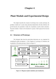
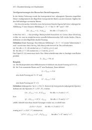
FIG. 1. Steady state EEDF at E/n g 100 Td. Comparison to a Maxwellian
distribution with same mean energy and dependence of the EEDF on the
ionization degree.
Maxwellian, depends strongly on E/n gas and weakly on the
plasma composition, i.e., the ionization degree. This is
shown in Figure 1 where the steady-state EEDF is shown for
E/n gas 100 Td in comparison to a Maxwellian distribution
with the same mean energy. Figure 1 also depicts the steadystate
EEDF for three different ionization degrees, showing
that larger electron fractions lead to a more Maxwellian-like
distribution. The other conditions for the EEDF calculations
are listed in the lower part of Table II.
It is important to note that the contribution of electron–
electron collisions cannot be neglected Figure 1. For the
precalculation of the rate constants, we follow the procedure
described in Sec. II B. All the Arrhenius parameters are
listed in Table I. The values of reaction G8 and G9 are estimates
taken from Ref. 9. We will compare results using
these fit values with the fully coupled solution in the next
section.
B. Dependence of the results on model assumptions
We calculate the steady-state solution using three different
levels of sophistication:
i fully coupled solution of Eq. 6 for the EEDF and
Eqs. 1 and 2 for the mass fractions,
ii precalculation of the EEDF under typical conditions
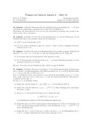
FIG. 3. Electron temperature as a function of power.
by Eq. 6, determination of the rate-constants, afterwards
solution of Eqs. 1 and 2 and the electron
temperature Eq. 22,
iii assumption of a Maxwellian distribution, calculation
of the rate constants by numerical integration, then
solving Eqs. 1, 2, and 22.
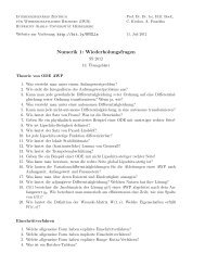
A comparison of the three methods is shown in Figure 2
where the concentration of electrons is plotted against the
power. It can be seen that precalculated EEDF and fully
coupled solution go well along the whole power range, while
the assumption of a Maxwellian distribution overestimates
the concentration. The reason is that the tail of the EEDF,
when calculated by solving the BE, is smaller than that of a
Maxwellian, leading to less electrons with high energies and
thus to lower ionization rates. In Figure 3 we observe similar
results for the electron temperature: While there are only
slight deviations between fully coupled and precalculated
calculations, the equilibrium assumption predicts about 1 eV
lower temperatures over the whole power range.
The dependence of the electron concentration on pressure
is shown in Figure 4. The precalculated EEDF method differs
from the fully coupled solution at very low pressures
about 1 Pa and below. The reason is that at such pressures
the ionization degree is much larger 1%–10% than the
0.1% being assumed for the EEDF calculations. This error
FIG. 2. Electron concentration as a function of power.
FIG. 4. Electron concentration as a function of pressure.
J. Vac. Sci. Technol. A, Vol. 16, No. 3, May/Jun 1998

1565 Ahlrichs, Riedel, and Warnatz : Spatially-averaged model for plasma etch processes 1565
While the situation for the gas phase is rather satisfying as
cross sections are known for all important reactions of a
chlorine plasma, and the nonequilibrium behavior of the
electrons can be accessed theoretically, there is little data
available for surface reactions. This situation gets even
worse when noticing the strong dependence of the plasma
composition on the corresponding sticking coefficients. 21
Here, more work should be done on detailed models for surface
reactions.
FIG. 5. Electron temperature as a function of pressure.
ACKNOWLEDGEMENT
The authors thank Deutsche Forschungsgemeinschaft
DFG for financial support.
can be avoided by introducing a fit function which is also
dependent on the ionization degree. The high ionization degree
drives the EEDF towards a Maxwellian, 9 thus the assumption
of a Maxwellian EEDF should become better at
low pressures, which can be verified from Figure 4 and also
from Figure 5, where the electron temperature is plotted
against system pressure.
IV. CONCLUSION
A simple model to simulate the characteristics of plasmaprocessing
reactors has been presented. The central assumption
of neglecting spatial dependencies leads to a computationally
efficient method to investigate the chemical kinetics
in such reactors. Incorporation of the model into spatially
resolved simulations should pose no principal problems. The
model consists of conservation equations for the plasma species
and a finite-differenced Boltzmann equation for the
EEDF. Both fully coupled solution and precalculation of the
EEDF and reaction rates is possible. A comparison of both
methods yields only slight differences for the plasma composition,
while the computational demands are considerably
lower if the EEDF is precalculated. Only if the nominal
plasma conditions especially the ionization degree used to
predetermine the EEDF are of an order of magnitude different
from the actual ones, there are considerable differences.
The assumption of a Maxwellian distribution, however, leads
to an overestimation in reaction rates which change results
by up to a factor of 2.
The predictive capability of a 0D model is largely determined
by the kinetic data for gas phase and surface reactions.
1 M. A. Lieberman and A. J. Lichtenberg, Principles of Plasma Discharges
and Materials Processing Wiley, New York, 1994.
2 M. Meyyappan, in ‘‘Computational Modeling in Semiconductor Processing,’’
Plasma Process Modeling, edited by M. Meyyappan Artech
House, Boston, 1995, Ch. 5.
3 M. J. Kushner, W. Z. Collision, M. J. Grapperhaus, J. P. Holand, and M.
S. Barnes, J. Appl. Phys. 80, 1337 1996.
4 U. Maas and J. Warnatz, Combust. Flame 74, 531988.
5 J. M. Smith, Chemical Engineering Kinetics McGraw–Hill, New York,
1981.
6 G. L. Rogoff, J. M. Kramer, and R. B. Piejak, Trans. Plasma Sci. 14, 103
1986.
7 R. S. Wise, D. P. Lymberopoulos, and D. J. Economou, Plasma Sources
Sci. Technol. 4, 317 1995.
8 M. Meyyappan, Vacuum 47, 215 1996.
9 E. Meeks and J. W. Shon, IEEE Trans. Plasma Sci. 23, 539 1995.
10 P. Jiang and D. J. Economou, J. Appl. Phys. 73, 8151 1993.
11 S. C. Deshmukh and D. J. Economou, J. Appl. Phys. 72, 4597 1992.
12 I. P. Shkarofsky, T. W. Johnston, and M. P. Bachynski, The Particle
Kinetics of Plasmas Addison-Wesley, Reading, MA, 1966.
13 L. W. Morgan, Comput. Phys. Commun. 58, 127 1990.
14 Y. Raizer, Gas Discharge Physics Springer, New York, 1991.
15 R. Winkler, H. Deutsch, J. Wilhelm, and C. Wilke, Beitr. Plasmaphys. 24,
285 1984.
16 R. Winkler, H. Deutsch, J. Wilhelm, and C. Wilke, Beitr. Plasmaphys. 24,
303 1984.
17 S. D. Rockwood, Phys. Rev. A 8, 2348 1973.
18 E. Meeks, H. K. Moffat, J. F. Grcar, and R. J. Kee, ‘‘AURORA: A
FORTRAN Program for Modeling Well Stirred Plasma and Thermal Reactors
with Gas and Surface Reactions.’’ Sandia National Laboratories
Report SAND96-8218, 1996.
19 F. A. Stevie and M. J. Vasile, J. Chem. Phys. 74, 5106 1981.
20 W. L. Morgan to be published.
21 E. Meeks, J. W. Shon, Y. Ra, and R. Jones, J. Vac. Sci. Technol. A 13,
2884 1995.
22 P. Deuflhard, E. Hairer, and J. Zugk, Numer. Math. 51, 501 1987.
23 P. Deuflhard and U. Nowak, Prog. Sci. Comput. 7, 371987.
24 Y. Ra and C.-H. Chen, J. Vac. Sci. Technol. A 11, 2911 1993.
JVST A - Vacuum, Surfaces, and Films