Complete Lecture Notes (PDF, 1.8 MB) - Institute for Theoretical ...
Complete Lecture Notes (PDF, 1.8 MB) - Institute for Theoretical ...
Complete Lecture Notes (PDF, 1.8 MB) - Institute for Theoretical ...

Create successful ePaper yourself
Turn your PDF publications into a flip-book with our unique Google optimized e-Paper software.
Quantum Field Theory I<br />
ETH Zurich, HS12<br />
Chapter 0<br />
Prof. N. Beisert<br />
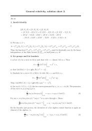
0 Overview<br />
Quantum Field Theory is the quantum theory of fields just like Quantum<br />
Mechanics describes quantum particles. Here, a the term “field” refers to one of<br />
the following:<br />
• A field of a classical field theory, such as Electromagnetism.<br />
• A wave function of a particle in Quantum Mechanics. This is why QFT is<br />
sometimes called “Second Quantisation”.<br />
• A smooth approximation to some property in a solid, e.g. the displacement of<br />
atoms in a lattice.<br />
• Some function of space and time describing some physics.<br />
Usually, excitations of the quantum field will be described by “particles”. In QFT<br />
the number of these particles is not conserved, they are created and annihilated<br />
when they interact. It is precisely what we observe in elementary particle physics,<br />
hence QFT has become the mathematical framework <strong>for</strong> this discipline.<br />
This lecture series gives an introduction to the basics of quantum field theory. It<br />
describes how to quantise the basic types of (relativistic) fields, how to handle<br />
their quantum operators and how to treat (sufficiently weak) interactions.<br />
Furthermore, we discuss symmetries, infinities and running couplings. The goal of<br />
the course is a derivation of particle scattering processes in basic QFT models.<br />
The continuation of this lecture course, QFT II, introduces an alternative<br />
quantisation framework, the path integral. 1 It is applied towards <strong>for</strong>mulating the<br />
Standard Model of Particle Physics by means of non-abelian gauge theory and<br />
spontaneous symmetry breaking.<br />
What Else is QFT?<br />
Many points of view.<br />
After attending this course, you may claim QFT is all about another 1000 ways to<br />
treat free particles and harmonic oscillators. True, some of the few systems we can<br />
solve exactly in theoretical physics; everything else is approximation. Physics, not<br />
maths!<br />
Look more carefully: QFT is a very rich subject, can learn about many things,<br />
some of which have attained a mythological status:<br />
• anti-particles, anti-matter,<br />
• vacuum energy,<br />
• tachyons,<br />
• ghosts,<br />
1 Path integral much more convenient to use than canonical quantisation discussed here. However,<br />
some important concepts are not as obvious as in canonical quantisation, e.g. notion of<br />
particles, scattering and importantly unitarity.<br />
1
• infinities,<br />
• mathematically inconsistent (?).<br />
Infinities.<br />
How to deal with infinities?<br />
Quote Dirac about QED (1975): “I must say that I am very dissatisfied with the<br />
situation, because this so-called ‘good theory’ does involve neglecting infinities<br />
which appear in its equations, neglecting them in an arbitrary way. This is just<br />
not sensible mathematics. Sensible mathematics involves neglecting a quantity<br />
when it is small — not neglecting it just because it is infinitely great and you do<br />
not want it!”<br />
Almost true, but it’s neither neglecting nor in an arbitrary way.<br />
Infinities are one reason why QFT is claimed to be mathematically ill-defined or<br />
even inconsistent. Yet QFT is a well-defined and consistent calculational<br />
framework to predict certain particle observables to extremely high precision.<br />
Many points of view, one is that it’s our own fault: QFT is somewhat idealised,<br />
assumes infinitely extended fields (IR) with infinite spatial resolution (UV); 2 no<br />
wonder that the theory produces infinities. Still, better to stick to idealised<br />
assumptions and live with infinities than use enormous discrete systems (actual<br />
solid state systems).<br />
A physics reason why these infinities can be absorbed somehow: Our observable<br />
everyday physics should neither depend on how large the universe actually is (IR)<br />
nor on how smooth or coarse-grained space is (UV).<br />
Can use infinities to learn about allowable particle interactions. Leads to curious<br />
effects: running coupling and quantum anomalies.<br />
More later (towards the end of the semester).<br />
Uniqueness. A related issue is uniqueness of the <strong>for</strong>mulation. Alike QM, QFT<br />
does not have a unique or universal <strong>for</strong>mulation.<br />
For instance, many meaningful things in QM/QFT are actually equivalence classes<br />
of objects. More convenient to work with specific representatives of these classes.<br />
Have to bear in mind that only equivalence class is meaningful, hence many ways<br />
to describe the same physical object.<br />
Usage of classes goes further, not just classes objects. Often have to consider<br />
classes of models rather than specific models. Something we have to accept,<br />
something QFT <strong>for</strong>ces upon us.<br />
We’ll notice that QFT does what it wants, not necessarily what we want. Cannot<br />
expect to get what we want using bare input parameters. Different <strong>for</strong>mulations of<br />
the same model naively may give different results. Must learn to adjust the input<br />
to the desired output, then find agreement. Just have to make sure that there is<br />
more output than input, otherwise QFT would be nice but meaningless exercise.<br />
2 Two sources <strong>for</strong> infinities: UV and IR.<br />
2
Nice feature: Can hide infinities there in a self-consistent way.<br />
Enough. Just some words of warning: Must give up some views on physics you<br />
have become used to. Only then you can understand something new. 3 Let’s start<br />
with something concrete. Discuss the tricky issues when they arise.<br />
Important Concepts.<br />
• unitarity – probabilistic framework.<br />
• locality – interactions are strictly local.<br />
• causality – special relativity.<br />
• symmetries – exciting algebra and geometry.<br />
• analyticity – complex analysis.<br />
0.1 Prerequisites<br />
• Classical mechanics (brief review in first lecture)<br />
• Quantum mechanics (brief review in first lecture)<br />
• Electrodynamics (as a simple classical field theory)<br />
• Mathematical methods in physics (HO, Fourier trans<strong>for</strong>ms, . . . )<br />
0.2 Contents<br />
1. Classical and Quantum Mechanics (2 lectures)<br />
2. Classical Free Scalar Field (3 lectures)<br />
3. Scalar Field Quantisation (5 lectures)<br />
4. Symmetries (5 lectures)<br />
5. Free Spinor Field (8 lectures)<br />
6. Free Vector Field (6 lectures)<br />
7. Interactions (4 lectures)<br />
8. Correlation Functions (6 lectures)<br />
9. Particle Scattering (4 lectures)<br />
10. Scattering Matrix (5 lectures)<br />
11. Loop Corrections (5 lectures)<br />
Indicated are the approximate number of 45-minute lectures. Altogether, the<br />
course consists of 54 lectures which includes one overview lecture.<br />
0.3 References<br />
There are many text books and lecture notes on quantum field theory. Here is a<br />
selection of well-known ones:<br />
• M. E. Peskin, D. V. Schroeder, “An Introduction to Quantum Field Theory”,<br />
Westview Press (1995)<br />
3 E.g. in special relativity: space and time become space time.<br />
3
• C. Itzykson, J.-B. Zuber, “Quantum Field Theory”, McGraw-Hill (1980)<br />
• P. Ramond, “Field Theory: A Modern Primer”, Westview Press (1990)<br />
• M. Srendnicki, “Quantum Field Theory”, Cambridge University Press (2007)<br />
• M. Kaku, “Quantum Field Theory”, Ox<strong>for</strong>d University Press (1993)<br />
• online: D. Tong, “Quantum Field Theory”, lecture notes,<br />
http://www.damtp.cam.ac.uk/user/tong/qft.html<br />
• online: M. Gaberdiel, “Quantenfeldtheorie”, lecture notes (in German),<br />
http://www.itp.phys.ethz.ch/people/gaberdim<br />
• . . .<br />
Peskin & Schroeder may be closest to this lecture course. 4<br />
4 We will not follow Peskin & Schroeder literally.<br />
4
Quantum Field Theory I<br />
ETH Zurich, HS12<br />
Chapter 1<br />
Prof. N. Beisert<br />
1 Classical and Quantum Mechanics<br />
To familiarise ourselves with the basics, let us review some elements of classical<br />
and quantum mechanics. Then we shall discuss some problems of combining<br />
quantum mechanics with special relativity.<br />
1.1 Classical Mechanics<br />
Consider a classical non-relativistic particle in a potential. Described by position<br />
variables q i (t) and action functional S[q] 1 2<br />
S[q] =<br />
A typical Lagrangian function is<br />
∫ t2<br />
with mass m and V (q) external potential.<br />
t 1<br />
dt L(q i (t), ˙q i (t), t) (1.1)<br />
L(⃗q, ˙⃗q) = 1 2 m ˙⃗q 2 − V (⃗q). (1.2)<br />
A classical path extremises (minimises) the action S. Determine saddle-point<br />
δS = 0 by variation of the action 3<br />
δS =<br />
=<br />
∫ t2<br />
t<br />
∫<br />
1<br />
t2<br />
t 1<br />
dt<br />
(<br />
δq i (t) ∂L<br />
∂q + δ i ˙qi (t) ∂L )<br />
∂ ˙q i<br />
( ∂L<br />
∂q − d )<br />
∂L<br />
+<br />
i dt ∂ ˙q i<br />
dt δq i (t)<br />
First term is equation of motion (Euler–Lagrange)<br />
δS<br />
δq i (t) = ∂L<br />
∂q − d i dt<br />
∫ t=t2<br />
t=t 1<br />
(<br />
d δq i (t) ∂L )<br />
!<br />
= 0 (1.3)<br />
∂ ˙q i<br />
∂L<br />
= 0. (1.4)<br />
∂ ˙q<br />
i<br />
Second term due to partial integration is boundary e.o.m., usually ignore. 4<br />
Example. Harmonic oscillator (free particle <strong>for</strong> ω = 0)<br />
L(⃗q, ˙⃗q) = 1 2 m ˙⃗q 2 − 1 2 mω2 ⃗q 2 , −m(¨⃗q + ω 2 ⃗q) = 0. (1.5)<br />
1 L is often time-independent: L(q i , ˙q i , t) = L(q i , ˙q i ).<br />
2 A single time derivative ˙q i usually suffices.<br />
3 Einstein summation convention: there is an implicit sum over all values <strong>for</strong> pairs of equal<br />
upper/lower indices.<br />
4 Usually fix position q i (t k ) = const. (Dirichlet) or momentum ∂L/∂ ˙q i (t k ) = 0 (Neumann) at<br />
boundary.<br />
1.1
1.2 Hamiltonian Formulation<br />
The Hamiltonian framework is the next step towards canonical quantum<br />
mechanics.<br />
Define conjugate momentum p i as 5<br />
and solve <strong>for</strong> ˙q i = ˙q i (q, p, t). 6 Define phase space as (q i , p i ).<br />
p i = ∂L<br />
∂ ˙q i (1.6)<br />
Lagrangian function L(q, ˙q, t) replaced by Hamiltonian function H(q, p, t) on phase<br />
space. Define H(q i , p i , t) as Legendre trans<strong>for</strong>mation of L<br />
H(q, p, t) = p i ˙q i (q, p, t) − L(q, ˙q(q, p, t), t). (1.7)<br />
Let us express e.o.m. through H. General variation reads<br />
δH = δp i ˙q i − δq i ∂L<br />
∂q i (<strong>1.8</strong>)<br />
where we substituted definition of momenta p i twice. Use Euler–Lagrange<br />
equation and momenta to simplify further<br />
δH = δp i ˙q i − δq i ṗ i . (1.9)<br />
Now, Hamiltonian e.o.m. ˙q i = ∂H/∂p i and ṗ i = −∂H/∂q i .<br />
Introduce Poisson brackets <strong>for</strong> functions f, g on phase space<br />
{f, g} := ∂f<br />
∂q i<br />
∂g<br />
− ∂f<br />
∂p i ∂p i<br />
Express time evolution <strong>for</strong> phase space functions f(p, q, t) 7<br />
Works well <strong>for</strong> f = q i and f = p i .<br />
df<br />
dt = ∂f<br />
∂t<br />
∂g<br />
∂q i . (1.10)<br />
− {H, f}. (1.11)<br />
Example.<br />
Harmonic oscillator<br />
⃗p = m ˙⃗q,<br />
Hamiltonian equations of motion<br />
˙⃗q = −{H, ⃗q} = ∂H<br />
∂⃗p = 1 m ⃗p,<br />
H = ⃗p· ˙⃗q − m 2 ˙⃗q 2 + mω2<br />
2 ⃗q 2 = 1<br />
2m ⃗p 2 + m 2 ω2 ⃗q 2 . (1.12)<br />
5 This is a choice, could also use different factors or notations.<br />
6 Suppose the equation can be solved <strong>for</strong> ˙q.<br />
7 The Hamiltonian H is a phase space function.<br />
˙⃗p = −{H, ⃗p} = −<br />
∂H<br />
∂⃗q = −mω2 ⃗q. (1.13)<br />
1.2
Convenient change of variables<br />
⃗a =<br />
1<br />
√<br />
2mω<br />
(mω⃗q + i⃗p) , ⃗a ∗ =<br />
1<br />
√<br />
2mω<br />
(mω⃗q − i⃗p) , (1.14)<br />
with new Poisson brackets<br />
{f, g} = −i ∂f<br />
∂a i<br />
∂g<br />
∂a ∗ i<br />
+ i ∂f<br />
∂a ∗ i<br />
∂g<br />
∂a i . (1.15)<br />
Separated first-order time evolution <strong>for</strong> ⃗a,⃗a †<br />
H = ω⃗a † ⃗a, ˙⃗a = −iω⃗a, ˙⃗a † = +iω⃗a † . (1.16)<br />
1.3 Quantum Mechanics<br />
In canonical quantisation classical objects are replaced by elements of linear<br />
algebra:<br />
• The state (q i , p i ) becomes a vector |ψ〉 in a Hilbert space V .<br />
• A phase space function f becomes a linear operator F on V .<br />
• Poisson brackets {f, g} become commutators −i −1 [F, G]. 8<br />
State equation of motion (Schrödinger), wave equation<br />
i d |ψ(t)〉 = H|ψ(t)〉. (1.17)<br />
dt<br />
Probabilistic role of wave function: |〈φ|ψ〉| 2 is probability. Requires:<br />
• 〈ψ|ψ〉 is positive.<br />
• 〈ψ|ψ〉 can be normalised to 1 by scaling |ψ〉.<br />
• 〈ψ|ψ〉 is conserved<br />
d<br />
dt 〈ψ|ψ〉 = (i)−1 〈ψ|(H − H † )|ψ〉 = 0. (1.18)<br />
Hamiltonian is hermitian (self-adjoint). Unitary time evolution:<br />
|ψ(t 2 )〉 = U(t 2 , t 1 )|ψ(t 1 )〉.<br />
• 〈ψ|F |ψ〉 is expectation value of operator F . Obeys classical time evolution.<br />
Example.<br />
Harmonic oscillator, free particle.<br />
Momentum operator and Hamiltonian 9<br />
⃗p = −i ∂ ( ) 2<br />
∂⃗q , [qi , p j ] = iδj, i H = − 2 ∂<br />
+ mω2<br />
2m ∂⃗q 2 ⃗q 2 . (1.19)<br />
8 Cannot always be translated literally, but up to simpler terms.<br />
9 Note: ⃗p = −i ⃗ ∂⃗q vs. E = +i∂ t . On wave function |ψ〉 = ∫ d d ⃗q ψ(⃗q, t)|⃗q〉, however: ⃗p|ψ〉 =<br />
+i ∫ d d ⃗q ⃗ ∂ψ(⃗q, t)|⃗q〉 and E|ψ〉 = +i ∫ d d ⃗q ∂ t ψ(⃗q, t)|⃗q〉<br />
1.3
Free particle: momentum eigenstate (Fourier trans<strong>for</strong>ms)<br />
∫<br />
|⃗p〉 =<br />
∫<br />
d d ⃗q e −i−1⃗p·⃗q |⃗q〉, |⃗q〉 =<br />
|⃗p〉 is energy eigenstate with E = ⃗p 2 /2m.<br />
Harmonic oscillator: use operators a i and a † i<br />
(<br />
1<br />
⃗a = √ mω⃗q + ∂ 2mω ∂⃗q<br />
with commutators<br />
)<br />
, ⃗a † =<br />
d d ⃗p<br />
(2π) d ei−1 ⃗p·⃗q |⃗p〉. (1.20)<br />
(<br />
1<br />
√ mω⃗q − ∂ )<br />
, (1.21)<br />
2mω ∂⃗q<br />
[a i , a † j ] = δi j. (1.22)<br />
Quantum Hamiltonian has extra vacuum energy E 0 = 1 2 dω<br />
H = 1 2 ωai a † i + 1 2 ωa† i ai = ω⃗a † ⃗a + 1 2 dω = ω⃗a† ⃗a + E 0 . (1.23)<br />
• Can add any E 0 to Hamiltonian. No effect. E 0 is irrelevant. Unless: E couples<br />
to something else (e.g. gravity).<br />
• Same effect as adding iα(⃗q·⃗p − ⃗p·⃗q) to H. 10 Classically invisible. Quantum<br />
energy shift ∆E 0 = −dα. Quantum ordering ambiguity. Harmless, affects<br />
trivial E 0 .<br />
• Quantum theory does as it pleases, e.g. introduce/shift E 0 . Best to consider all<br />
allowable terms in the first place.<br />
Construct spectrum: Start from vacuum state |0〉 to be annihilated by ⃗a (has<br />
energy E = E 0 , but irrelevant)<br />
a i |0〉 = 0. (1.24)<br />
Add excitations n i ≥ 0 and normalise state 〈⃗n|⃗n〉 = 1<br />
( d∏<br />
)<br />
(a † i<br />
|⃗n〉 =<br />
)n i<br />
√ |0〉. (1.25)<br />
ni<br />
i=1<br />
Energy eigenstate with E = ωN + E 0 where N = ∑ d<br />
i=1 n i is total excitation<br />
number. Crucial property<br />
[H,⃗a † ] = ω⃗a † . (1.26)<br />
1.4 Quantum Mechanics and Relativity<br />
Let us set = 1, c = 1 <strong>for</strong> convenience. 11<br />
Attempts to set up a relativistic version of quantum mechanics have failed. Let us<br />
see why.<br />
10 No ambiguity <strong>for</strong> ⃗p 2 and ⃗q 2 , but useful to consider all second degree polynomials in ⃗p and ⃗q.<br />
11 Can be recovered from considerations of physical units.<br />
1.4
Non-relativistic and relativistic energy relation<br />
e = ⃗p 2<br />
2m , vs. e2 = ⃗p 2 + m 2 or e = √ ⃗p 2 + m 2 . (1.27)<br />
Natural guess <strong>for</strong> relativistic wave equation (Klein–Gordon)<br />
( ( ) 2 ( ) )<br />
2 ∂ ∂<br />
− + − m 2 |ψ〉 = 0. (1.28)<br />
∂t ∂⃗q<br />
Has several conceptual problems:<br />
Probabilistic Properties. The norm 〈ψ|ψ〉 of non-relativistic QM is conserved<br />
only <strong>for</strong> first-order wave equation.<br />
There is a real conserved quantity<br />
Problem:<br />
Q =<br />
i<br />
2m<br />
• Q is not positive definite.<br />
• Not suitable <strong>for</strong> probabilistic interpretation! 12<br />
(〈ψ| ∂ ∂t |ψ〉 − ∂ ∂t 〈ψ|ψ〉 )<br />
, (1.29)<br />
One can define a positive definite measure, but it is not local.<br />
Why consider probabilities in a time slice in the first place?<br />
Causality.<br />
Consider the overlap<br />
〈⃗q 2 |U(t 2 , t 1 )|⃗q 1 〉 (1.30)<br />
<strong>for</strong> a pair of spacetime points (t 1 , q 1 ) and (t 2 , q 2 ). Probability amplitude <strong>for</strong><br />
particle moving from 1 to 2.<br />
Problem:<br />
• Overlap non-zero if points are space-like separated.<br />
• <strong>for</strong>bidden region: violation of causality?<br />
• at least: exponential suppression (tunnelling).<br />
Negative-Energy Solutions. Second-order wave equation. For every<br />
positive-energy solution<br />
∫<br />
|⃗p, +, t〉 = d d ⃗q e −i⃗p·⃗q−ie(⃗p)t |⃗q〉 (1.31)<br />
there is a negative-energy solution<br />
∫<br />
|⃗p, −, t〉 =<br />
d d ⃗q e −i⃗p·⃗q+ie(⃗p)t |⃗q〉. (1.32)<br />
Problems:<br />
12 As we shall see, Q is rather similar to an electric charge.<br />
1.5
• Negative-energy particles not observed. 13<br />
• Positive-energy particle could fall to negative-energy state. A lot of energy<br />
released to produce other particles.<br />
Could insist on positive energies by wave equation<br />
i ∂ ( ) 2 ∂<br />
√−<br />
∂t |ψ〉 = + m<br />
∂⃗q<br />
2 |ψ〉. (1.33)<br />
Problems:<br />
• Square root of operator hard to define.<br />
• Certainly non-local wave-equation.<br />
Particle Creation.<br />
of particles.<br />
Special relativity allows energy to be converted to rest mass<br />
• Relativistic quantum mechanics should allow such processes.<br />
• Quantum mechanics usually assumes a fixed particle number.<br />
Dirac Equation.<br />
problems<br />
The Dirac equation was an attempt to overcome some<br />
∂<br />
|ψ〉 = ∂<br />
αk |ψ〉 + βm|ψ〉. (1.34)<br />
∂t ∂qk Relativistic wave equation; implies Klein–Gordon equation.<br />
Probabilistic interpretation:<br />
• First-order wave equation.<br />
• 〈ψ|ψ〉 is conserved and positive definite.<br />
• Positivity requires Bose statistics.<br />
Spin:<br />
• Operators α k imply spin-1/2 particles.<br />
• No spin-0 particles reproducible.<br />
• Half-integer spin requires Fermi statistics.<br />
Negative-energy solutions:<br />
• Exist (with different spin d.o.f.).<br />
• Separation from positive energies is non-local.<br />
Dirac equation has the same problems as Klein–Gordon.<br />
Conclusion.<br />
Klein–Gordon and Dirac equations:<br />
• Perfectly acceptable relativistic wave equations.<br />
• No probabilistic interpretation.<br />
• Model without particle production.<br />
13 Extract energy from making particle faster!<br />
1.6
1.5 Conventions<br />
Units. We shall work with natural units = c = 1.<br />
• c = 299 792 458 m s −1 there<strong>for</strong>e s := 299 792 458 m.<br />
• = 1.055 . . . × 10 −34 kg m 2 s −1 there<strong>for</strong>e kg := 2.843 . . . × 10 42 m −1 .<br />
• can always reinstall appropriate units by inserting 1 = c = .<br />
• particle physics unit electron Volt (eV): m = 5.068 × 10 6 eV −1 ,<br />
s = 1.519 × 10 15 eV −1 , kg = 5.610 × 10 35 eV.<br />
• convert back to SI units:<br />
eV = 5.068 × 10 6 m −1 = 1.519 × 10 15 s −1 = 1.783 × 10 −36 kg.<br />
Euclidean space.<br />
Write a three-vector x as<br />
• x j with Latin indices k, l, · · · = 1, 2, 3.<br />
• ⃗x = (x 1 , x 2 , x 3 ) = (x, y, z).<br />
Scalar product between two vectors<br />
⃗a·⃗b :=<br />
3∑<br />
a k b k = a 1 b 1 + a 2 b 2 + a 3 b 3 . (1.35)<br />
k=1<br />
Vector square<br />
⃗a 2 := ⃗a·⃗a = a 2 1 + a 2 2 + a 2 3. (1.36)<br />
Totally anti-symmetric epsilon-tensor ε ijk with normalisation<br />
ε 123 = +1. (1.37)<br />
Use to define cross product<br />
(a × b) k = ε ijk a i b j . (1.38)<br />
Minkowski Space. Four vectors, Greek indices µ, ν, . . . = 0, 1, 2, 3:<br />
• position vector x µ := (x 0 , x 1 , x 2 , x 3 ) = (t, ⃗x).<br />
• momentum covector p µ := (p 0 , p 1 , p 2 , p 3 ) = (e, ⃗p).<br />
Summation convention: repeated index µ means implicit sum over µ = 0, 1, 2, 3<br />
x µ p µ :=<br />
3∑<br />
x µ p µ = et + ⃗x·⃗p. (1.39)<br />
µ=0<br />
Minkowski metric: signature (−+++)<br />
Raise and lower indices (wherever needed):<br />
η µν = η µν = diag(−1, +1, +1, +1). (1.40)<br />
x µ := η µν x µ = (−t, ⃗x), p µ := η µν p µ = (−e, ⃗p). (1.41)<br />
1.7
Scalar products of two vectors or two covectors, e.g.<br />
Our conventions:<br />
p·p := −e 2 + ⃗p 2 . (1.42)<br />
• Mass shell p 2 = −m 2 : p 2 < 0 massive, p 2 = 0 massless, p 2 > 0 tachyonic.<br />
• Light cone: (x − y) 2 < 0 time-like, (x − y) 2 = 0 light-like, (x − y) 2 > 0 space-like.<br />
(1.43)<br />
Why?<br />
• notation follows space (not time). x µ = (t,⃗x) p µ<br />
= (t,⃗x)<br />
• x i = x i but x 0 = −x 0 = t.<br />
• p i = p i but p 0 = −p 0 = e.<br />
• Wick rotations natural: just rotate time t → it and obtain Euclidean metric.<br />
How to convert?<br />
• flip sign of every η µν and η µν .<br />
• find out which (co)vectors match: x µ and p µ agree literally, x µ and p µ flip the<br />
sign.<br />
• flip sign <strong>for</strong> every scalar product of vectors of same type: e.g.<br />
p 2 + m 2 ↔ −p 2 + m 2 .<br />
• preserve scalar product between different vectors: x µ p µ . 14<br />
• note: ⃗p opposite sign compared to Peskin & Schroeder; mild problem: sign of ⃗p<br />
and e is merely convention.<br />
Name Spaces. We have only 26 Latin letters at our disposal and some are more<br />
attractive than others. Have to recycle:<br />
• e may be 2.71 . . ., but also energy,<br />
• π may be 3.14 . . ., but also momentum conjugate to field φ,<br />
• i may be √ −1, but also useful <strong>for</strong> counting.<br />
• κ may look like k or K on the blackboard.<br />
14 There<strong>for</strong>e also x·p unchanged (two signs cancel).<br />
<strong>1.8</strong>
• H may be Hamilton function or operator.<br />
• . . .<br />
Will typically not say explicitly which letter means what:<br />
• May even use same letter <strong>for</strong> different meanings in one <strong>for</strong>mula.<br />
• Can guess meaning from the context, e.g. i in exp(πi . . .) vs. ∑ n<br />
i=1 .<br />
• Indices typically do not mix with other symbols.<br />
• Could try to avoid, but may also clutter notation.<br />
• It’s a fact of life (and the literature).<br />
1.9
Quantum Field Theory I<br />
ETH Zurich, HS12<br />
Chapter 2<br />
Prof. N. Beisert<br />
2 Classical Free Scalar Field<br />
In the following we shall discuss one of the simplest field theory models, the<br />
classical non-interacting relativistic scalar field.<br />
2.1 Spring Lattice<br />
Be<strong>for</strong>e considering field, start with an approximation we can certainly handle:<br />
lattice.<br />
Consider an atomic lattice:<br />
• 1D or 2D cubic lattice,<br />
• atoms are coupled to neighbours by springs, 1<br />
• atoms are coupled to rest position by springs,<br />
• atoms can move only orthogonally to lattice (transverse),<br />
• boundaries: periodic identification.<br />
(2.1)<br />
model parameters and variables:<br />
• lattice separation r,<br />
• number of atoms N (in each direction),<br />
• mass of each atom µ,<br />
• lattice spring constant κ,<br />
• return spring constant λ,<br />
• shift orthogonal to lattice q j,k<br />
Lagrangian Formulation.<br />
Lagrange function<br />
L = L kin − V lat − V rest (2.2)<br />
1 Springs are useful approximations because they model first deviation from rest position; always<br />
applies to small excitations.<br />
2.1
Standard non-relativistic kinetic terms<br />
L kin = 1 2 µ N<br />
∑<br />
i,j=1<br />
Potential <strong>for</strong> springs between atoms (ignore x, y-potential) 2<br />
˙q 2 i,j. (2.3)<br />
V lat = 1κ ∑ N<br />
(q<br />
2 i−1,j − q i,j ) 2 + 1κ ∑ N<br />
(q<br />
2 i,j−1 − q i,j ) 2 . (2.4)<br />
i,j=1<br />
i,j=1<br />
Some spring potential to drive atoms back to rest position<br />
V rest = 1λ ∑ N<br />
q 2 2 i,j. (2.5)<br />
i,j=1<br />
Quadratic in q’s: bunch of coupled HO’s. Equations of motion<br />
µ¨q i,j<br />
− κ(q i−1,j − 2q i,j + q i+1,j )<br />
− κ(q i,j−1 − 2q i,j + q i,j+1 ) + λq i,j = 0. (2.6)<br />
Note: spatially homogeneous equations. Use discrete Fourier trans<strong>for</strong>m to solve<br />
(respect periodicity)<br />
q i,j (t) = 1 ∑ N (<br />
c<br />
√ k,l<br />
exp − 2πi<br />
)<br />
N 2 2µωk,l N (ki + lj) − iω k,lt<br />
k,l=1<br />
+ 1<br />
N 2<br />
N<br />
∑<br />
k,l=1<br />
c ∗ ( )<br />
k,l 2πi<br />
√ exp<br />
2µωk,l N (ki + lj) + iω k,lt<br />
Used freedom to define coefficients c k,l to introduce prefactors.Complex conjugate<br />
coefficients c ∗ k,l in second term ensure reality of q i,j. Note: c ∗ k,l represents mode of<br />
opposite momentum and energy w.r.t. c k,l !<br />
E.o.m. translates to dispersion relation:<br />
µω 2 k,l = λ + 4κ sin 2 πk<br />
N<br />
(2.7)<br />
+ 4κ sin2<br />
πl<br />
N . (2.8)<br />
(2.9)<br />
2 Can ignore due to d 2 = d 2 x + d 2 y + d 2 z, shifts potential by an irrelevant constant. Moreover<br />
longitudinal and transverse excitations decouple.<br />
2.2
Hamiltonian Formulation.<br />
Derive Hamiltonian function as Legendre trans<strong>for</strong>m of L<br />
Define momenta<br />
p i,j := ∂L<br />
∂ ˙q i,j<br />
= µ ˙q i,j . (2.10)<br />
H = H kin + V lat + V rest with H kin = 1<br />
2µ<br />
Then define canonical Poisson brackets<br />
N∑<br />
( ∂f<br />
{f, g} :=<br />
i,j=1<br />
∂q i,j<br />
∂g<br />
− ∂f<br />
∂p i,j ∂p i,j<br />
In other words {q i,j , p j,k } = δ i,k δ j,l and {q, q} = {p, p} = 0.<br />
N∑<br />
p 2 i,j. (2.11)<br />
i,j=1<br />
)<br />
∂g<br />
. (2.12)<br />
∂q i,j<br />
Fourier Modes.<br />
a k,l =<br />
Introduce new complex variables (Fourier trans<strong>for</strong>m)<br />
1<br />
√<br />
2µωk,l<br />
N<br />
∑<br />
i,j=1<br />
exp<br />
Trans<strong>for</strong>med Hamiltonian is very simple<br />
H = 1<br />
N 2<br />
( 2πi<br />
N (ki + lj) )<br />
(µωk,l<br />
q i,j + ip i,j<br />
)<br />
. (2.13)<br />
N<br />
∑<br />
k,l=1<br />
Poisson brackets <strong>for</strong> new variables are simple, too<br />
{a i,j , a ∗ k,l} = −i N 2 δ i,k δ j,l ,<br />
Can convince oneself that equations of motion hold<br />
and solved by above Lagrangian solution<br />
ω k,l a ∗ k,la k,l . (2.14)<br />
{a i,j , a k,l } = {a ∗ i,j, a ∗ k,l} = 0. (2.15)<br />
ȧ k,l = −{H, a k,l } = −iω k,l a k,l ,<br />
ȧ ∗ k,l = −{H, a ∗ k,l} = +iω k,l a ∗ k,l. (2.16)<br />
a k,l (t) = c k,l exp(−iω k,l t), a ∗ k,l(t) = c ∗ k,l exp(+iω k,l t). (2.17)<br />
2.2 Continuum Limit<br />
Now turn this spring lattice into a smooth field ϕ:<br />
• send number of sites N → ∞.<br />
• box of size L in all directions; lattice separation r = L/N → 0.<br />
• positions x = ir = iL/N,<br />
• field q i,... = ϕ(⃗x),<br />
• generalise to d spatial dimensions, e.g. d = 1, 2, 3.<br />
Some useful rules<br />
N∑<br />
→ 1 ∫<br />
r<br />
i=1<br />
dx, q i − q i−1 → r(∂ϕ) (2.18)<br />
2.3
Lagrangian Formulation. Substitute this in Lagrangian<br />
∫ ( µ<br />
L → d d ⃗x<br />
2r d ˙ϕ2 −<br />
κ<br />
2r (⃗ ∂ϕ) 2 − λ )<br />
d−2 2r d ϕ2 . (2.19)<br />
Diverges as r → 0, but can rescale parameters. Suitable rescalings<br />
µ = r d¯µ, κ = r d−2¯κ, λ = r d¯λ, (2.20)<br />
Parameters become densities. Lagrangian functional<br />
∫ (<br />
L[ϕ, ˙ϕ](t) = d d 1<br />
⃗x ¯µ 2 ˙ϕ2 − 1 ¯κ(⃗ ∂ϕ) 2 − 1 ¯λϕ<br />
)<br />
2 . (2.21)<br />
2 2<br />
Can furthermore rescale field ϕ = ¯κ −1/2 φ<br />
∫<br />
L[φ, ˙φ](t)<br />
(<br />
= d d 1<br />
⃗x<br />
2 ¯µ¯κ−1 ˙φ2 − 1(⃗ ∂φ) 2 − 1 ¯λ¯κ<br />
)<br />
−1 φ 2 . (2.22)<br />
2 2<br />
Derive e.o.m.: start with action functional S[φ]<br />
∫<br />
∫<br />
S[φ] = dt L[φ](t) = dt d d ⃗x L ( φ(⃗x, t), ∂ i φ(⃗x, t), ˙φ(⃗x, t) ) ; (2.23)<br />
useful to express (homogeneous) Lagrange functional L[φ](t) through Lagrangian<br />
density L(φ, ⃗ ∂φ, ˙φ) (the Lagrangian).<br />
Vary action functional (discard boundary terms)<br />
∫ ( ∂L<br />
δS[φ] = dt d d ⃗x δφ<br />
∂φ − ∂ ∂L<br />
∂x i ∂(∂ i φ) − d dt<br />
Write general Euler–Lagrange equation <strong>for</strong> fields<br />
In our case<br />
∂L ∂<br />
(⃗x, t) −<br />
∂φ ∂x i<br />
∂L<br />
∂(∂ i φ) (⃗x, t) − d dt<br />
)<br />
∂L<br />
∂ ˙φ<br />
+ . . .<br />
!<br />
= 0. (2.24)<br />
∂L<br />
(⃗x, t) = 0. (2.25)<br />
∂ ˙φ<br />
− ¯µ¯κ −1 ¨φ + ⃗ ∂ 2 φ − ¯λ¯κ −1 φ = 0; (2.26)<br />
agrees with continuum limit of discrete e.o.m.. Now denote as speed of light c and<br />
mass m<br />
¯µ¯κ −1 = c −2 = 1, ¯λ¯κ −1 = m 2 , (2.27)<br />
to discover Klein–Gordon equation (set c = 1)<br />
− c −2 ¨φ + ⃗ ∂ 2 φ − m 2 φ = 0. (2.28)<br />
2.4
Plane Wave Solutions. Consider solutions on infinite space and time.<br />
Homogeneous equation solved by Fourier trans<strong>for</strong>mation<br />
∫<br />
d d ⃗p<br />
φ(⃗x, t) =<br />
(2π) d 2e(⃗p) α(⃗p) exp( −i⃗p·⃗x − ie(⃗p)t )<br />
∫<br />
d d ⃗p<br />
+<br />
(2π) d 2e(⃗p) α∗ (⃗p) exp ( +i⃗p·⃗x + ie(⃗p)t ) (2.29)<br />
with (positive) energy e(⃗p) on mass shell (often called ω(⃗p))<br />
Agrees with discrete solution identifying momenta as<br />
p = 2πk/L,<br />
e(⃗p) = √ ⃗p 2 + m 2 . (2.30)<br />
N∑<br />
→ L ∫<br />
2π<br />
k=1<br />
Some remarks on factors and conventions:<br />
dp, c k,... = α(⃗p) √<br />
2e(⃗p)r<br />
d . (2.31)<br />
• Fourier trans<strong>for</strong>ms on R produce factors of 2π, need to be put somewhere.<br />
Convention to associate (2π) −1 to every dp: ¯dp := dp/2π.<br />
No factors of 2π <strong>for</strong> dx. No factors of 2π in exponent.<br />
• Combination d d ⃗p/2e(⃗p) is a useful combination: Relativistic covariance. Reason<br />
<strong>for</strong> conversion factor in c k,... .<br />
2.3 Relativistic Covariance<br />
The Klein–Gordon equation can be written manifestly relativistically 3 4<br />
− ∂ µ ∂ µ φ + m 2 φ = −∂ 2 φ + m 2 φ = 0. (2.32)<br />
Also Lagrangian and action manifestly relativistic<br />
∫<br />
L = − 1 2 (∂φ)2 − 1 2 m2 φ 2 , S =<br />
d D x L. (2.33)<br />
To understand the relativistic behaviour of the solution, consider integration over a<br />
mass shell p 2 + m 2 = 0<br />
∫<br />
d D p δ(p 2 + m 2 )θ(p 0 ) f(p)<br />
∫<br />
= d d ⃗p de δ(−e 2 + ⃗p 2 + m 2 )θ(e) f(e, ⃗p)<br />
∫ d d ⃗p de<br />
= δ(e − √ ⃗p<br />
2e<br />
2 + m 2 )θ(e) f(e, ⃗p)<br />
∫ d d ⃗p<br />
= f(e(⃗p), ⃗p) (2.34)<br />
2e(⃗p)<br />
3 ∂ 2 often written as D’Alembertian □.<br />
4 Signature of spacetime is −+++!<br />
2.5
Solution is just Fourier trans<strong>for</strong>m<br />
∫<br />
φ(x) =<br />
with momentum space field defined on shell only<br />
d D p<br />
(2π) D φ(p) exp( −ip µ x µ) (2.35)<br />
φ(p) = 2πδ(p 2 + m 2 ) ( θ(p 0 )α(⃗p) + θ(−p 0 )α ∗ (−⃗p) ) . (2.36)<br />
Momentum space e.o.m. obviously satisfied<br />
(p 2 + m 2 )φ(p) = 0. (2.37)<br />
α(⃗p) and α ∗ (⃗p) define amplitudes on <strong>for</strong>ward/backward mass shells.<br />
(2.38)<br />
Note that φ(p) obeys reality condition (from φ(x) ∗ = φ(x))<br />
φ(p) ∗ = φ(−p). (2.39)<br />
2.4 Hamiltonian Field Theory<br />
Now that we have a nice relativistic <strong>for</strong>mulation <strong>for</strong> the Klein–Gordon field φ(x),<br />
let’s separate space from time. 5<br />
Position Space.<br />
Define momentum π (field) conjugate to φ<br />
π(⃗x, t) =<br />
Determine Hamiltonian<br />
∫<br />
H[φ, π] =<br />
∫<br />
=<br />
δL ∂L<br />
(t) =<br />
δ ˙φ(⃗x) ∂ ˙φ (⃗x, t) = ˙φ(⃗x, t). (2.40)<br />
d d ⃗x π ˙ϕ − L[φ, ˙φ]<br />
d d ⃗x<br />
(<br />
1<br />
2 π2 + 1 2 (⃗ ∂φ) 2 + 1 2 m2 φ 2 )<br />
. (2.41)<br />
5 Formalism breaks relativistic invariance, physics remains relativistic.<br />
2.6
Not relativistically covariant, not designed to be. 6<br />
Define Poisson brackets <strong>for</strong> phase space functionals f, g<br />
∫ ( δf<br />
{f, g} = d d δg<br />
⃗x<br />
δφ(⃗x) δπ(⃗x) − δf )<br />
δg<br />
. (2.42)<br />
δπ(⃗x) δφ(⃗x)<br />
Poisson brackets of fields yield delta-functions 7<br />
∫<br />
{φ(⃗x), π(⃗y)} = d d ⃗z δ d (⃗x − ⃗z)δ d (⃗y − ⃗z) = δ d (⃗x − ⃗z). (2.43)<br />
Momentum Space. Now introduce momentum modes 8<br />
∫<br />
a(⃗p) = d d ⃗x exp (i⃗p·⃗x) ( e(⃗p)φ(⃗x) + iπ(⃗x) ) , (2.44)<br />
and inverse Fourier trans<strong>for</strong>mation<br />
∫<br />
d d ⃗p<br />
φ(⃗x) =<br />
a(⃗p) exp(−i⃗p·⃗x)<br />
(2π) d 2e(⃗p)<br />
∫<br />
d d ⃗p<br />
+<br />
(2π) d 2e(⃗p) a∗ (⃗p) exp(+i⃗p·⃗x),<br />
π(⃗x) = − i ∫<br />
d d ⃗p<br />
a(⃗p) exp(−i⃗p·⃗x)<br />
2 (2π)<br />
d<br />
+ i ∫<br />
d d ⃗p<br />
2 (2π) d a∗ (⃗p) exp(+i⃗p·⃗x). (2.45)<br />
Compute Poisson brackets <strong>for</strong> Fourier modes 9 10<br />
In other words<br />
{f, g} = −i(2π) d ∫<br />
{a(⃗p), a ∗ (⃗q)} = −i 2e(⃗p) (2π) d δ d (⃗p − ⃗q). (2.46)<br />
( δf<br />
d d ⃗p 2e(⃗p)<br />
δa(⃗p)<br />
Hamiltonian translates to<br />
H = 1 ∫<br />
d d ∫<br />
⃗p<br />
2 (2π) d a∗ (⃗p)a(⃗p) =<br />
Hence e.o.m. <strong>for</strong> field oscillator<br />
One HO <strong>for</strong> every momentum. Solution<br />
δg<br />
δa ∗ (⃗p) −<br />
ȧ(⃗p) = −{H, a(⃗p)} = −ie(⃗p)a(⃗q),<br />
δf<br />
δa ∗ (⃗p)<br />
)<br />
δg<br />
. (2.47)<br />
δa(⃗p)<br />
d d ⃗p<br />
(2π) d 2e(⃗p) e(⃗p)a∗ (⃗p)a(⃗p). (2.48)<br />
ȧ ∗ (⃗p) = −{H, a ∗ (⃗p)} = +ie(⃗p)a ∗ (⃗q). (2.49)<br />
a(⃗p, t) = α(⃗p) exp(−ie(⃗p)t), a ∗ (⃗p, t) = α ∗ (⃗p) exp(+ie(⃗p)t). (2.50)<br />
6 Hamiltonian governs time translation.<br />
7 Formula <strong>for</strong> variation δφ(⃗x)/δφ(⃗z) = δ d (⃗x − ⃗z).<br />
8 Have some additional factors compared to some literature.<br />
9 Conventional 2π <strong>for</strong> delta-function in momentum space.<br />
10 Factor 2e(⃗p) appropriate relativistic measure <strong>for</strong> mass shell.<br />
2.7
Quantum Field Theory I<br />
ETH Zurich, HS12<br />
Chapter 3<br />
Prof. N. Beisert<br />
3 Scalar Field Quantisation<br />
We can now go ahead and try to quantise the classical scalar field using the<br />
canonical procedure described be<strong>for</strong>e. We will encounter some infinities, and<br />
discuss how to deal with them. Then we shall investigate a few basic objects in<br />
QFT.<br />
3.1 Quantisation<br />
Start with the Hamiltonian <strong>for</strong>mulation of the scalar field discussed earlier.<br />
Equal-Time Commutators. Phase space consists of the field φ(⃗x) and the<br />
conjugate momentum π(⃗x) with Poisson bracket 1<br />
{φ(⃗x), π(⃗y)} = δ d (⃗x − ⃗y). (3.1)<br />
Hence the canonical quantisation implies operators φ(⃗x) and π(⃗x)<br />
[φ(⃗x), π(⃗y)] = iδ d (⃗x − ⃗y). (3.2)<br />
Note that φ and π are now operator-valued fields (rather: distributions). 2<br />
Field States. Next have to define some states. Straight QM would lead to a<br />
state |φ 0 〉 <strong>for</strong> every field configuration φ 0 (⃗x) such that<br />
φ(⃗x)|φ 0 〉 = φ 0 (⃗x)|φ 0 〉,<br />
δ<br />
π(⃗x)|φ 0 〉 = −i<br />
δφ 0 (⃗x) |φ 0〉. (3.3)<br />
Can be done <strong>for</strong>mally, but not so convenient. Sketch of an eigenstate<br />
∫ (<br />
|0〉 = Dφ exp − 1 ∫<br />
)<br />
d d ⃗x d d ⃗y Ω(⃗x, ⃗y) φ(⃗x) φ(⃗y) . (3.4)<br />
2<br />
1 At the moment, the fields are defined on a common time slice t, e.g. t = 0. Later we discuss<br />
unequal times.<br />
2 The delta-function is a distribution, also the fields should be considered distributions. Distributions<br />
are linear maps from test functions to numbers (or operators in this case). In physics, we<br />
write them as integrals with a distributional kernel (e.g. the delta-function). Sometimes we also<br />
per<strong>for</strong>m illegal operations (e.g. evaluate delta-function δ(x) at x = 0).<br />
3.1
Momentum Space. The classical field is a bunch of coupled HO’s, let us<br />
diagonalise them and use creation and annihilation operators.<br />
Go to momentum space, and pick a and a † appropriately, same trans<strong>for</strong>mation as<br />
above<br />
∫<br />
a(⃗p) = d d ⃗x exp (i⃗p·⃗x) ( e(⃗p)φ(⃗x) + iπ(⃗x) ) ,<br />
∫<br />
d d ⃗p<br />
φ(⃗x) =<br />
a(⃗p) exp(−i⃗p·⃗x)<br />
(2π) d 2e(⃗p)<br />
∫<br />
d d ⃗p<br />
+<br />
(2π) d 2e(⃗p) a† (⃗p) exp(+i⃗p·⃗x),<br />
π(⃗x) = − i ∫<br />
d d ⃗p<br />
a(⃗p) exp(−i⃗p·⃗x)<br />
2 (2π)<br />
d<br />
+ i ∫<br />
d d ⃗p<br />
2 (2π) d a† (⃗p) exp(+i⃗p·⃗x). (3.5)<br />
Commutation relations in momentum space<br />
[a(⃗p), a † (⃗q)] = 2e(⃗p) (2π) d δ d (⃗p − ⃗q). (3.6)<br />
Substitute fields into Hamiltonian paying attention to ordering<br />
H = 1 ∫<br />
d d ⃗p (<br />
a † (⃗p)a(⃗p) + a(⃗p)a † (⃗p) )<br />
4 (2π) d<br />
= 1 ∫<br />
d d ⃗p (<br />
2a † (⃗p)a(⃗p) + [a(⃗p), a † (⃗p)] )<br />
4 (2π) d<br />
= 1 ∫<br />
d d ⃗p<br />
2 (2π) d a† (⃗p)a(⃗p) + 1 ∫<br />
d d ⃗p e(⃗p) δ d (⃗p − ⃗p). (3.7)<br />
2<br />
Vacuum Energy. Introduce a vacuum state |0〉 annihilated by all a(⃗p). Two<br />
problems with vacuum energy H|0〉 = E 0 |0〉<br />
E 0 = 1 ∫<br />
d d ⃗p e(⃗p) δ d (⃗p − ⃗p) : (3.8)<br />
2<br />
• delta-function<br />
∫<br />
is δ d (⃗p − ⃗p) = δ d (0) is ill-defined,<br />
• integral 1 2 d d ⃗p e(⃗p) diverges.<br />
These are self-made problems:<br />
• We considered an infinite volume. Not reasonable to expect a finite energy. IR<br />
problem! The delta-function has units of volume. It measures the volume of the<br />
system δ d (⃗p − ⃗p) ∼ V → ∞. Consider energy density instead!<br />
∫<br />
• Integral 1 P<br />
2 0 dd ⃗p e(⃗p) represents vacuum energy density. Infinitely many<br />
oscillators per volume element, not reasonable to expect<br />
∫<br />
finite energy density.<br />
UV problem! Introduce cutoff |⃗p| < P to obtain 1 P<br />
2 0 dd ⃗p e(⃗p) ∼ P d+1 .<br />
Finite lattice has similar effect to regularise IR and UV.<br />
To avoid IR infinities in QFT:<br />
3.2
• Put the system in a finite box. Possible but inconvenient. Rather work with<br />
infinite system and cope with IR divergences. E.g. consider energy density.<br />
To avoid UV infinities in QFT:<br />
• By definition we want a field theory, not a discrete model. Physics: Should be<br />
able to approximate by discrete model.<br />
• Regularisation: impose momentum cut-off, consider a lattice, other tricks<br />
without physical motivation, . . .<br />
• Renormalisation: remove terms which would diverge.<br />
• Remove regularisation: obtain finite results.<br />
Here: simply drop E 0 .<br />
• There is no meaning to an absolute vacuum energy.<br />
• May add any constant to Hamiltonian (to compensate E 0 ).<br />
• Makes no observable difference in any physical process.<br />
• Vacuum energy only a philosophical or religious question.<br />
• Later on, infinities lead to interesting effects.<br />
Renormalised Hamiltonian H ren<br />
H ren := H − E 0 = 1 2<br />
∫<br />
d d ⃗p<br />
(2π) d a† (⃗p)a(⃗p). (3.9)<br />
Nice, vacuum has zero energy.<br />
Normal Ordering. The ordering of variables in classical H plays no role. In<br />
quantum theory it does! It is responsible <strong>for</strong> vacuum energy E 0 .<br />
How to map some classical observable O to a quantum operator?<br />
A possible map is normal ordering N(O):<br />
• Express O in terms of a and a ∗ → a † .<br />
• Write all a † ’s to the left of all a’s.<br />
Here, renormalised Hamiltonian is the normal ordering of H<br />
There are other ordering prescriptions <strong>for</strong> operators:<br />
H ren = N(H). (3.10)<br />
• Normal ordering depends on the choice of vacuum state. There may be other<br />
normal-ordering prescriptions associated to different “vacuum” states.<br />
• There are other useful ordering prescriptions which we will encounter, e.g. time<br />
ordering.<br />
3.2 Fock Space<br />
We have:<br />
• a collection of HO’s labelled by momentum ⃗p,<br />
3.3
• a vacuum state |0〉 with energy E = 0.<br />
Discuss other related states.<br />
Single-Particle States.<br />
Can now excite vacuum<br />
|⃗p〉 := a † (⃗p)|0〉. (3.11)<br />
Energy eigenstate with energy<br />
E = +e(⃗p). (3.12)<br />
Energy of a particle with momentum ⃗p and mass m.<br />
Negative-Energy Solutions.<br />
Note:<br />
• Energy is positive E > 0.<br />
• State a(⃗p)|0〉 would have negative energy.<br />
Problem of negative-energy particles solved!<br />
Does not exist by construction.<br />
• a † (⃗p) creates a particle of momentum ⃗p a positive energy +e(⃗p) from the<br />
vacuum. a † (⃗p) is particle creation operator.<br />
• a(⃗p) removes a particle of momentum ⃗p and thus removes the positive energy<br />
+e(⃗p) from the state.<br />
a(⃗p)|⃗q〉 = a(⃗p)a † (⃗q)|0〉 = [a(⃗p), a † (⃗q)]|0〉<br />
= 2e(⃗p) (2π) d δ d (⃗p − ⃗q) |0〉. (3.13)<br />
a(⃗p) is particle annihilation operator. 3 (3.14)<br />
Interpretation of position space operators not as straight:<br />
φ(⃗x) = φ † (⃗x) as well as π(⃗x) = π † (⃗x) create or annihilate a particle at position ⃗x.<br />
Result is typically superposition.<br />
3 a(⃗p) is not an anti-particle (although this is sometimes claimed). It has negative energy while<br />
anti-particles (like particles) have positive energy. For the real scalar, the particle is its own<br />
anti-particle.<br />
3.4
Normalisation.<br />
Let us define proper normalisation <strong>for</strong> the vacuum<br />
Normalisation of a single-particle state:<br />
〈0|0〉 = 1. (3.15)<br />
〈⃗p|⃗p〉 = 2e(⃗p) (2π) d δ d (⃗p − ⃗p) = ∞. (3.16)<br />
Known problem from QM: Plane-wave states have infinite extent, smeared over all<br />
space, unphysical. Recall δ d (⃗p − ⃗p) represents volume of space.<br />
Consider peaked wave packet state |f〉 (test function) instead<br />
∫<br />
d d p f(⃗p)<br />
|f〉 :=<br />
|⃗p〉. (3.17)<br />
(2π) d 2e(⃗p)<br />
For suitable f(⃗p) this state has a finite normalisation<br />
∫ d d p |f(⃗p)| 2<br />
〈f|f〉 =<br />
(2π) d 2e(⃗p) . (3.18)<br />
Multi-Particle States and Fock Space. Now excite more than one harmonic<br />
oscillator<br />
|⃗p 1 , ⃗p 2 , . . . , ⃗p n 〉 := a † (⃗p 1 ) a † (⃗p 2 ) · · · a † (⃗p n ) |0〉. (3.19)<br />
The energy is given by the sum of particle energies 4<br />
E =<br />
n∑<br />
e(⃗p k ). (3.20)<br />
k=1<br />
All particles are freely interchangeable<br />
because creation operators commute<br />
|. . . , ⃗p, ⃗q, . . .〉 = |. . . , ⃗q, ⃗p, . . .〉 (3.21)<br />
[a † (⃗p), a † (⃗q)] = 0. (3.22)<br />
Bose statistics <strong>for</strong> indistinguishable particles: Wave function automatically totally<br />
symmetric in QFT.<br />
A generic QFT state (based on the vacuum |0〉) is a linear combination of<br />
k-particle states with k not fixed. This vector space is called Fock space. It is the<br />
direct sum<br />
V Fock = V 0 ⊕ V 1 ⊕ V 2 ⊕ V 3 ⊕ . . . , V n = (V 1 ) ⊗sn (3.23)<br />
of n-particle spaces V n where<br />
• V 0 = C merely contains the vacuum state |0〉.<br />
4 Use [H, a † (⃗p)] = e(⃗p)a † (⃗p) to show H|n〉 = Ha † 1 . . . a† n|0〉 = [H, a † 1 ]a† 2 . . . a† n|0〉 + . . . +<br />
a † 1 . . . a† n−1 [H, a† n]|0〉 = E|n〉.<br />
3.5
• V 1 = V particle is the space of single particle states |⃗p〉 with positive energy.<br />
• V n is the symmetric tensor product of n copies of V 1 .<br />
Consider non-relativistic physics:<br />
• The available energy is bounded from above. Much smaller than particle rest<br />
masses m = e(0).<br />
• Relevant part of Fock space with n bounded. For example: V 1 , V 2 or V 1 ⊕ V 2 .<br />
• Multiple-particle QM is a low-energy limit of QFT. Becomes QFT when number<br />
of particles is unbounded.<br />
Conservation Laws. The Hamiltonian H measures the total energy E.<br />
There is also a set of operators to measure total momentum P ⃗<br />
∫<br />
d<br />
⃗P d ⃗p<br />
:=<br />
(2π) d 2e(⃗p) ⃗p a† (⃗p)a(⃗p). (3.24)<br />
with eigenvalue P ⃗ = ∑ n<br />
k=1 ⃗p k on state |⃗p 1 , . . . ⃗p n 〉. Vacuum carries no momentum.<br />
Combine into relativistic vector P µ = (H, P ⃗ ) of operators<br />
∫<br />
P µ :=<br />
d d ⃗p<br />
(2π) d 2e(⃗p) p µ(⃗p) a † (⃗p)a(⃗p), p µ (⃗p) := (e(⃗p), ⃗p). (3.25)<br />
Another useful operator is the particle number operator n<br />
∫<br />
d d ⃗p<br />
N :=<br />
(2π) d 2e(⃗p) a† (⃗p)a(⃗p). (3.26)<br />
It measures the number of particles n in a state |⃗p 1 , . . . ⃗p n 〉<br />
NV n = nV n . (3.27)<br />
The relativistic momentum vector and the number operator are conserved<br />
Moreover, they carry no momentum<br />
[H, P µ ] = [H, N] = 0. (3.28)<br />
[P µ , P ν ] = [P µ , N] = 0. (3.29)<br />
In fact, there are many conservation laws. Any two operators made from number<br />
density operators commute<br />
n(⃗p) := a † (⃗p)a(⃗p), [n(⃗p), n(⃗q)] = 0. (3.30)<br />
Hence such operators are conserved, carry no momentum and no particle number:<br />
[H, n(⃗p)] = [P µ , n(⃗p)] = [N, n(⃗p)] = 0. (3.31)<br />
In a free theory there are infinitely many conservation laws. 5<br />
5 Should not say this: Free theory is trivial.<br />
3.6
3.3 Complex Scalar Field<br />
Let us discuss a slightly more elaborate case of the scalar field, the complex scalar,<br />
where we first encounter anti-particles.<br />
The complex scalar field φ(x) has the Lagrangian 6 7<br />
L = −∂ µ φ ∗ ∂ µ φ − m 2 φ ∗ φ = −|∂φ| 2 − m 2 |φ| 2 . (3.32)<br />
For the conjugate momentum we obtain 8<br />
π = ∂L<br />
∂ ˙φ = ˙φ ∗ ,<br />
π ∗ = ∂L<br />
∂ ˙φ ∗ = ˙φ. (3.33)<br />
In the quantum theory we then impose the canonical commutators<br />
[φ(⃗x), π(⃗y)] = [φ(⃗x) † , π(⃗y) † ] = iδ(⃗x − ⃗y). (3.34)<br />
The equation of motion associated to the above Lagrangian is the very same<br />
Klein–Gordon equation. However, now complex solutions φ(x) are allowed. Field<br />
operators (with time dependence, see below) now read:<br />
∫<br />
d d ⃗p<br />
φ(x) =<br />
b(⃗p) exp(−ip·x)<br />
(2π) d 2e(⃗p)<br />
∫<br />
d d ⃗p<br />
+<br />
(2π) d 2e(⃗p) a† (⃗p) exp(+ip·x),<br />
∫<br />
φ † d d ⃗p<br />
(x) =<br />
a(⃗p) exp(−ip·x)<br />
(2π) d 2e(⃗p)<br />
∫<br />
d d ⃗p<br />
+<br />
(2π) d 2e(⃗p) b† (⃗p) exp(+ip·x), (3.35)<br />
Note the strange appearance of a and b. For a ≠ b we have φ ≠ φ † while a = b<br />
implies a real field φ = φ † . Non-trivial commutation relations:<br />
[a(⃗p), a † (⃗q)] = [b(⃗p), b † (⃗q)] = 2e(⃗p) (2π) d δ d (⃗p − ⃗q). (3.36)<br />
and quantum Hamiltonian<br />
H ren := 1 2<br />
∫<br />
d d ⃗p<br />
(2π) d (<br />
a † (⃗p)a(⃗p) + b † (⃗p)b(⃗p) ) . (3.37)<br />
The complex scalar carries a charge, +1 <strong>for</strong> φ and −1 <strong>for</strong> φ † .<br />
6 The prefactor 1 2 of the real scalar field (φ2 ) is now absent. It is a convenient symmetry factor.<br />
Here the appropriate symmetry factor is 1 because φ ∗ ≠ φ. More on symmetry factors later.<br />
7 One can also set φ(x) = (φ 1 +iφ 2 )/ √ 2 and φ ∗ (x) = (φ 1 −iφ 2 )/ √ 2 and obtain two independent<br />
scalar fields with equal mass.<br />
8 One may just as well define π = ∂L/∂ ˙φ ∗ = ˙φ. It is a matter of convention, and makes no<br />
difference if applied consistently.<br />
3.7
• The operator a † creates a particle with charge +1.<br />
• The operator b has negative energy, it should remove a particle. The operator<br />
carries the same charge as a † , hence the corresponding particle should have<br />
charge −1.<br />
Two types of particles: particle and anti-particle. Opposite charges, but equal<br />
mass and positive energies. Conclusion:<br />
• a † creates a particle,<br />
• b annihilates an anti-particle,<br />
• b † creates an anti-particle,<br />
• a annihilates a particle,<br />
• vacuum annihilated by a’s and b’s.<br />
(3.38)<br />
3.4 Correlators<br />
Have quantised field. States have an adjustable number of indistinguishable<br />
particle with definite momentum. Now what? Consider particle propagation in<br />
space and time.<br />
Schrödinger Picture.<br />
Steps:<br />
• create a particle at x µ = (t, ⃗x),<br />
• let the state evolve <strong>for</strong> some time s − t,<br />
• measure the particle at y µ = (s, ⃗y).<br />
Could use φ(⃗x) or π(⃗x) to create particle from vacuum. 9 Use φ because π = ˙φ can<br />
be obtained from time derivative.<br />
In Schrödinger picture the states evolve in time<br />
i d |Ψ, t〉 = H |Ψ, t〉 (3.39)<br />
dt<br />
9 The operators also annihilate particles, but not from the vacuum.<br />
3.8
We solve this as 10 |Ψ, s〉 = exp ( −iH(s − t) ) |Ψ, t〉 (3.40)<br />
Altogether the correlator reads<br />
∆ + (y, x) = 〈0|φ(⃗y) exp ( −i(s − t)H ) φ(⃗x)|0〉.<br />
∫<br />
d d ⃗p<br />
=<br />
(2π) d 2e(⃗p) exp( −ip·(y − x) ) . (3.41)<br />
Space and time take different roles. Nevertheless, final answer is perfectly<br />
relativistic.<br />
Heisenberg Picture. Heisenberg picture makes relativistic properties more<br />
manifest. Translate time-dependence of state to time-dependence of operators<br />
F H (t) := exp ( +iH(t − t 0 ) ) F S (t) exp ( −iH(t − t 0 ) ) , (3.42)<br />
where t 0 is the reference time slice on which quantum states are defined, say<br />
t 0 = 0. States are there<strong>for</strong>e time-independent in Heisenberg picture<br />
Field φ in Heisenberg picture<br />
F S (t)|Ψ, t〉 = F S (t) exp ( −iH(t − t 0 ) ) |Ψ, t 0 〉<br />
= exp ( −iH(t − t 0 ) ) F H (t)|Ψ, t 0 〉. (3.43)<br />
φ(x) = φ(⃗x, t) = exp ( +iHt ) φ(⃗x) exp ( −iHt )<br />
∫<br />
d d ⃗p (<br />
=<br />
e −ip·x a(⃗p) + e +ip·x a † (⃗p) ) (3.44)<br />
(2π) d 2e(⃗p)<br />
• has complete spacetime dependence,<br />
• is manifestly relativistic,<br />
• no need to consider π = ˙φ,<br />
• obeys Klein–Gordon equation (∂ 2 − m 2 )∆ + = 0,<br />
• same <strong>for</strong>m as solution of Euler–Lagrange equations.<br />
Correlator from Heisenberg picture (vacuum always the same)<br />
∆ + (y, x) = 〈0|φ(y)φ(x)|0〉. (3.45)<br />
Same result, but more immediate and relativistic derivation.<br />
Correlator.<br />
Let us discuss the correlation function<br />
∫<br />
d d ⃗p<br />
∆ + (y, x) =<br />
(2π) d 2e(⃗p) exp( −ip·(y − x) ) . (3.46)<br />
10 H is time-independent, hence time-translation is governed simply by exp(−iH∆t). Later we<br />
shall encounter a more difficult situation.<br />
3.9
We know it in momentum space<br />
∫<br />
d d+1 p<br />
∆ + (y, x) =<br />
(2π) ∆ +(p) exp ( −ip·(y − x) ) .<br />
d+1<br />
∆ + (p) = 2πδ(p 2 + m 2 )θ(p 0 ) (3.47)<br />
How about position space?<br />
• Due to translation symmetry: ∆ + (y − x) = ∆ + (y, x).<br />
• Due to Lorentz rotations ∆ + (x) = m d−1 F (m 2 x 2 ).<br />
• Distinguish three regions: future, past, elsewhere.<br />
Klein–Gordon equation <strong>for</strong> F becomes<br />
4rF ′′ (r) + 2(d + 1)F ′ (r) − F (r) = 0 (3.48)<br />
This is DG <strong>for</strong> Bessel functions J α (z). 11 Two solutions:<br />
F ± (r) = r −(d−1)/4 J ±(d−1)/2 (i √ r). (3.49)<br />
First, consider future with x = (t, 0) where t = ± √ −x 2 . 12 Substitute in above<br />
momentum space expression<br />
∫<br />
d d ⃗p<br />
∆ + (x) =<br />
(2π) d 2e(⃗p) exp( −ite(⃗p) ) .<br />
= Vol(Sd−1 )<br />
2(2π) d<br />
∫ ∞<br />
0<br />
∫ ∞<br />
dp p d−1<br />
√<br />
p2 + m 2 exp( −it √ p 2 + m 2) .<br />
= Vol(Sd−1 )<br />
de(e 2 − m 2 ) (d−2)/2 exp(−ite)<br />
2(2π) d m<br />
∼ e −imt <strong>for</strong> t → ±∞. (3.50)<br />
Oscillation with positive frequency m. Same <strong>for</strong> past. Fixes linear combination of<br />
F ± (Hankel H α ) 13<br />
∆ + (y − x) ∼<br />
For space-like separation<br />
m(d−1)/2<br />
(y − x) H ( √ )<br />
(d−1)/2 (d−1)/2 m −(y − x)<br />
2<br />
. (3.51)<br />
∆ + (x) ∼ e −mr <strong>for</strong> r = √ x 2 → ∞. (3.52)<br />
Non-zero, but exponentially decaying (range m). Fixes linear combination of F ±<br />
(modified Bessel K α )<br />
∆ + (y − x) ∼<br />
m(d−1)/2<br />
(y − x) K ( √ )<br />
(d−1)/2 (d−1)/2 m (y − x)<br />
2<br />
. (3.53)<br />
11 Bessel functions are well-known solutions <strong>for</strong> spherical waves.<br />
12 Can go to such a frame with x = (t, 0).<br />
13 The asymptotic behaviour e −imt determines which of the two Hankel functions H (1) and H (2)<br />
applies to past and future.<br />
3.10
Same as in relativistic QM. Causality?<br />
Be<strong>for</strong>e we discuss causality, let us summarise in this figure:<br />
(3.54)<br />
Note that there are also delta-function contributions <strong>for</strong> light-like separation.<br />
Unequal-Time Commutator.<br />
measured.<br />
Okay to violate causality as long as not<br />
Correct question: Can one measurement at x influence the other at y? Consider<br />
commutator<br />
∆(y − x) := [φ(y), φ(x)]. (3.55)<br />
We can relate to above correlators by inserting between vacua<br />
Observation:<br />
∆(y − x) = 〈0|[φ(y), φ(x)]|0〉 = ∆ + (y − x) − ∆ + (x − y). (3.56)<br />
• ∆ + is symmetric <strong>for</strong> space-like separations,<br />
• φ(x) and φ(y) commute <strong>for</strong> space-like separations,<br />
• follows also from invariance and equal-time commutator,<br />
• causality preserved.<br />
Note: two contributions cancel <strong>for</strong> space-like separations:<br />
• Particle created at x and annihilated at y cancels against<br />
• particle created at y and annihilated at x.<br />
However, commutator non-trivial <strong>for</strong> time-like separations<br />
∆(y − x) ∼<br />
m(d−1)/2<br />
(y − x) J ( √ )<br />
(d−1)/2 (d−1)/2 m −(y − x)<br />
2<br />
. (3.57)<br />
Time-like separated measurements can influence each other.<br />
Finally we can recover equal-time commutators. For two fields φ the commutator<br />
follows from symmetry of the integral<br />
∫<br />
∆(0, ⃗y − ⃗x) =<br />
d d ⃗p (<br />
e −i⃗p·(⃗y−⃗x) − e i⃗p·(⃗y−⃗x)) = 0. (3.58)<br />
(2π) d 2e(⃗p)<br />
3.11
The commutator between a field φ and its conjugate π yields<br />
∂<br />
∂x ∆(0, ⃗y − ⃗x) = i ∫<br />
d d ⃗p (<br />
e −i⃗p·(⃗y−⃗x) + e i⃗p·(⃗y−⃗x)) = iδ d (⃗x − ⃗y) (3.59)<br />
0 2 (2π) d<br />
in agreement with the fundamental commutator [φ(⃗y), π(⃗x)].<br />
3.5 Sources<br />
We have a free field, we have discussed correlators of two fields, but there is not<br />
much else we can do besides adding interactions (later).<br />
As a first step towards interactions, let us discuss driving the field by an external<br />
source ρ(x)<br />
− ∂ 2 φ(x) + m 2 φ(x) = ρ(x). (3.60)<br />
The source is non-zero only <strong>for</strong> some finite interval of time.<br />
Question: Given an initial field φ i (x) obeying the homogeneous Klein–Gordon<br />
equation, how to determine the solution φ(x) of inhomogeneous Klein–Gordon<br />
equation such that φ(x) = φ i (x) <strong>for</strong> all t < t 0 be<strong>for</strong>e activation of the source at t 0 ?<br />
In particular, what is the final field φ f (x) which must also obey the homogeneous<br />
Klein–Gordon equation.<br />
(3.61)<br />
Due to linearity we make the ansatz 14<br />
∫<br />
φ(x) = φ i (x) + ∆φ(x), ∆φ(x) =<br />
d d+1 y G R (x − y) ρ(y) (3.62)<br />
where G R is the retarded propagator or Green(’s) function<br />
− ∂ 2 G R (x) + m 2 G R (x) = δ d+1 (x), G R (x) = 0 <strong>for</strong> x 0 < 0. (3.63)<br />
The first equation is conveniently solved in momentum space<br />
∫<br />
d d+1 p<br />
G(x) = e−ip·x G(p) (3.64)<br />
(2π) d+1<br />
with Klein–Gordon equation and solution 15<br />
p 2 G(p) + m 2 G R (p) = 1, G(p) =<br />
1<br />
p 2 + m 2 . (3.65)<br />
14 Admittedly, this is a perfectly classical problem already encountered in electrodynamics.<br />
15 As such, this solution is in fact slightly ill-defined, second condition resolves the ambiguities<br />
as we shall see.<br />
3.12
Let us see how to incorporate the second relation. Write as<br />
∫<br />
d d ∫<br />
⃗p de<br />
G(x) = e−i⃗p·⃗x −1<br />
(2π) d 2π e−iet<br />
e 2 − e(⃗p) 2<br />
∫<br />
d d ∫ ( )<br />
⃗p de<br />
= e−i⃗p·⃗x −1 e<br />
−iet<br />
(2π) d 2π 2e(⃗p) e − e(⃗p) −<br />
e−iet<br />
. (3.66)<br />
e + e(⃗p)<br />
Solve Fourier integrals by residue theorem in complex plane. The integral over e<br />
runs from −∞ to +∞; close contour! This is done by a semi-circle in the complex<br />
plane with very large radius. Contribution must vanish, consider exponent:<br />
Only second term suppresses contribution:<br />
exp(−iet) = exp(−it Re e) exp(t Im e). (3.67)<br />
• For t > 0 we need Im e < 0: Close contour in lower half.<br />
• For t < 0 we need Im e > 0: Close contour in upper half.<br />
(3.68)<br />
We have two poles at e = ±e(⃗p) on the real axis = contour. Need to decide how<br />
they contribute to residues.<br />
For retarded propagator, we want G R (x) = 0 <strong>for</strong> t < 0. Achieved by shifting poles<br />
slightly into lower half plane 16 1<br />
G R (p) =<br />
p 2 + m 2 − ip 0 ɛ . (3.69)<br />
(3.70)<br />
No poles in upper half plane, hence G R (x) <strong>for</strong> t < 0. For t > 0, however, both<br />
16 Alternatively, de<strong>for</strong>m contour to close above points.<br />
3.13
poles contribute a residue, we obtain<br />
∫<br />
d d ⃗p (<br />
G R (x) = iθ(t)<br />
e −ip·x − e +ip·x)<br />
(2π) d 2e(⃗p)<br />
= iθ(t) ( ∆ + (x) − ∆ + (−x) ) = iθ(t)∆(x). (3.71)<br />
Nice: relation between correlation functions and propagators. Yields position<br />
space <strong>for</strong>m <strong>for</strong> propagator.<br />
Confirm that it satisfies defining relation: 17<br />
(−∂ 2 + m 2 )G R (x) = iθ(t) (−∂ 2 + m 2 )∆(x) + ∂ ( )<br />
iδ(t) ∆(x)<br />
∂t<br />
+ iδ(t) ∆(x) ˙ = δ d+1 (x). (3.72)<br />
• First term vanishes because ∆ is on shell.<br />
• Second term vanishes because [φ(⃗x), φ(⃗y)] = 0.<br />
• Third term uses [φ(⃗x), φ(⃗y)] = iδ d (⃗x − ⃗y).<br />
We can now determine the contribution to φ from the source. Let us focus on the<br />
future after the source is switched off 18<br />
∫<br />
∆φ(x) = i d d+1 y ∆(x − y) ρ(y). (3.73)<br />
Trans<strong>for</strong>m this to momentum space with<br />
∫<br />
d d+1 p<br />
ρ(x) = e−ip·x ρ(p), ρ(p) ∗ = ρ(−p) (3.74)<br />
(2π) d+1<br />
yields<br />
∫<br />
∆φ(x) =<br />
d d ⃗p (<br />
ie −ip·x ρ(p) − ie +ip·x ρ ∗ (p) ) . (3.75)<br />
(2π) d 2e(⃗p)<br />
As we know the homogeneous Klein–Gordon equation is solved by<br />
∫<br />
d d ⃗p (<br />
φ i (x) =<br />
a(⃗p)e −ip·x + a † (⃗p)e ip·x) . (3.76)<br />
(2π) d 2e(⃗p)<br />
Let this represent the solution in the distant past. Then the solution φ f in the<br />
distant future is obtained by replacing<br />
a(⃗p) ↦→ a(⃗p) + iρ(e(⃗p), ⃗p). (3.77)<br />
We notice that only the Fourier modes of the source ρ on the mass shell can<br />
actually drive the field φ.<br />
We can now ask how much energy, momentum or particle number the source ρ<br />
transfers to the field, e.g.<br />
∆E = 〈0|H(t > t 1 )|0〉 − 〈0|H(t < t 0 )|0〉. (3.78)<br />
17 Distribute the derivatives in a suitable way between θ and ∆.<br />
18 Can there<strong>for</strong>e set θ(y 0 − x 0 ) = 1.<br />
3.14
The contributions from the quantum modes a, a † drop out. What remains is<br />
manifestly positive <strong>for</strong> E = P 0 and N 19<br />
∫<br />
∆P µ =<br />
∫<br />
∆N =<br />
d d ⃗p<br />
(2π) d 2e(⃗p) p µ(⃗p) |ρ(⃗p)| 2 ,<br />
d d ⃗p<br />
(2π) d 2e(⃗p) |ρ(⃗p)|2 . (3.79)<br />
19 ∆N is not manifestly integer <strong>for</strong> an external field. However, if ρ is quantum, ρ † (⃗p)ρ(⃗p) should<br />
again lead to an integer ∆N.<br />
3.15
Quantum Field Theory I<br />
ETH Zurich, HS12<br />
Chapter 4<br />
Prof. N. Beisert<br />
4 Symmetries<br />
So far we have not discussed symmetries. QFT does not actually need symmetries,<br />
but they help very much in restricting classes of models, providing stability and<br />
simplifying calculations as well as results. 1<br />
For example, in most cases QFT’s have some symmetry of space and time.<br />
Particularly in fundamental particle physics all models have relativistic invariance<br />
or Poincaré symmetry.<br />
Symmetries are some trans<strong>for</strong>mations of the fields φ → φ ′ that map solutions of<br />
the equations of motion to other solutions. Hence they can be used to generate a<br />
whole class of solutions from a single one.<br />
We shall discuss the action of various types of symmetries, their groups and<br />
representations, and the resulting conserved charges via Noether’s theorem. Most<br />
of the discussion applies to classical and quantum field theories.<br />
4.1 Internal Symmetries<br />
Let us first discuss internal symmetries. In a QFT with several fields, these<br />
typically trans<strong>for</strong>m the fields into each other in some way without making<br />
reference to their dependence on space or time.<br />
The simplest example is a complex scalar field φ(x) with Lagrangian and<br />
corresponding equation of motion<br />
L = −∂ µ φ ∗ ∂ µ φ − m 2 φ ∗ φ,<br />
Consider a global trans<strong>for</strong>mation of the fields<br />
∂ 2 φ − m 2 φ = 0,<br />
∂ 2 φ ∗ − m 2 φ ∗ = 0.<br />
(4.1)<br />
φ ′ (x) = e +iα φ(x), φ ∗ ′ (x) = e −iα φ ∗ (x). (4.2)<br />
It maps a solution of the equations of motion to another solution 2<br />
∂ 2 φ ′ − m 2 φ ′ = e iα ( ∂ 2 φ − m 2 φ ) = 0. (4.3)<br />
Moreover the symmetry leaves the Lagrangian and the action invariant<br />
L(φ ′ , ∂ µ φ ′ ) = L(φ, ∂ µ φ), S[φ ′ ] = S[φ]. (4.4)<br />
1 For free particles symmetries are not that helpful, the true power of symmetries arises in<br />
interacting situations.<br />
2 The trans<strong>for</strong>med field φ ′ satisfies the equation of motion because φ does. Same <strong>for</strong> complex<br />
conjugate field φ ∗ .<br />
4.1
Any such trans<strong>for</strong>mation must be a symmetry because it maps extrema of the<br />
action to extrema and hence solutions to solutions. Symmetries of the action are<br />
more powerful than mere symmetries of the equations of motion. In the following<br />
we will only consider symmetries of the action. 3<br />
Noether’s Theorem. Every continuous global symmetry of the action leads to<br />
a conserved current and thus a conserved charge <strong>for</strong> solutions of the equations of<br />
motion.<br />
Let us derive the theorem: Consider a solution φ of the equations of motion. By<br />
construction, any variation of the Lagrangian is a total derivative 4<br />
δL = δL<br />
δφ δφ + δL<br />
δ(∂ µ φ) ∂ µδφ<br />
= ∂ µ<br />
δL<br />
δ(∂ µ φ) δφ +<br />
δL<br />
( ) δL<br />
δ(∂ µ φ) ∂ µδφ = ∂ µ<br />
δ(∂ µ φ) δφ . (4.5)<br />
Suppose now δφ is the infinitesimal field variation of a continuous symmetry. We<br />
know that δS = 0, hence the Lagrangian can only change by some total derivative<br />
Equating the two expressions <strong>for</strong> δL we find a current 5<br />
J µ =<br />
which is conserved <strong>for</strong> every solution φ<br />
δL = δα ∂ µ J µ 0 . (4.6)<br />
δL<br />
δ(∂ µ φ)<br />
δφ<br />
δα − J µ 0 (4.7)<br />
∂ µ J µ = 0. (4.8)<br />
Furthermore, a conserved current implies a conserved charge<br />
∫<br />
Q(t) = d d ⃗x J 0 (t, ⃗x) (4.9)<br />
if we assume that the field vanishes sufficiently fast at spatial infinity<br />
∫<br />
∫<br />
˙Q = d d ⃗x ∂ 0 J 0 = − d d ⃗x ∂ k J k = 0. (4.10)<br />
The conserved charge actually generates an infinitesimal symmetry trans<strong>for</strong>mation<br />
via the Poisson brackets<br />
[Q, F ] = − δF<br />
(4.11)<br />
δα<br />
as can be shown using its defining relations.<br />
3 For example the scaling trans<strong>for</strong>mation φ(x) → e β φ(x) also maps solutions to solutions, but<br />
it rescales the Lagrangian L ′ = e 2β L. If one considers QFT’s to be specified by their Lagrangians,<br />
then this symmetry of the equations of motion relates two different models L and L ′ . We typically<br />
us the freedom to redefine the fields to bring the Lagrangian in some canonical <strong>for</strong>m.<br />
4 Usually we can ignore this term, here it is relevant.<br />
5 Any term of the <strong>for</strong>m ∂ ν B µν with antisymmetric indices on B µν can be added to J µ without<br />
modifying any of the following relations.<br />
4.2
Example.<br />
by<br />
Let us consider the complex scalar field. The field variation is defined<br />
δφ = iφ δα, δφ ∗ = −iφ ∗ δα. (4.12)<br />
The Lagrangian is invariant under the trans<strong>for</strong>mation δL = 0, hence J µ 0 = 0. The<br />
other term reads<br />
J µ =<br />
δL<br />
δ(∂ µ φ)<br />
δφ<br />
δα +<br />
The naive divergence of the current reads<br />
δL δφ ∗<br />
δ(∂ µ φ ∗ ) δα<br />
= (−∂ µ φ ∗ ) (iφ) + (−∂ µ φ) (−iφ ∗ )<br />
= −i(∂ µ φ ∗ φ − φ ∗ ∂ µ φ). (4.13)<br />
∂ µ J µ = −i(∂ 2 φ ∗ φ − φ ∗ ∂ 2 φ). (4.14)<br />
This indeed vanishes <strong>for</strong> a solution of the equations of motion.<br />
The conserved charge reads<br />
∫<br />
∫<br />
Q = i d d ⃗x ( ˙φ ∗ φ − φ ∗ ˙φ) = i<br />
d d ⃗x (πφ − φ ∗ π ∗ ). (4.15)<br />
Trans<strong>for</strong>med to momentum space we get<br />
∫<br />
d d ⃗p (<br />
Q =<br />
a ∗ (⃗p)a(⃗p) − b ∗ (⃗p)b(⃗p) ) . (4.16)<br />
(2π) d 2e(⃗p)<br />
This charge is indeed time-independent and (Poisson) commutes with the<br />
Hamiltonian. As expected, it obeys<br />
{Q, φ} = −iφ = − δφ<br />
δα ,<br />
We furthermore observe a relation to the number operators<br />
{Q, φ∗ } = +iφ ∗ = − δφ∗<br />
δα . (4.17)<br />
Q = N a − N b . (4.18)<br />
In the quantum theory, Q there<strong>for</strong>e measures the number of particles created by a †<br />
minus the number of particles created by b † .<br />
Despite the similarities, there is a crucial difference to the number operator: The<br />
charge Q is associated to a symmetry, whereas a single number operator N is not. 6<br />
In a symmetric theory with interactions, Q is conserved while N is in general not.<br />
Quantum Action. Let us briefly state how to represent this symmetry in the<br />
quantum theory where Q = N a − N b becomes a quantum operator. It is obviously<br />
hermitian<br />
Q † = Q. (4.19)<br />
6 One might construct a non-local symmetry trans<strong>for</strong>mation corresponding the number operator<br />
in a free field theory. However, this symmetry would not generalise to interactions.<br />
4.3
It obeys the following commutation relations with creation and annihilation<br />
operators<br />
[Q, a(x)] = −a(x),<br />
[Q, b(x)] = +b(x),<br />
[Q, a † (x)] = +a † (x), [Q, b † (x)] = −b † (x). (4.20)<br />
This tells us that particles of type a carry positive unit charge while the<br />
antiparticles of type b carry negative unit charge.<br />
The commutators of spacetime fields φ ∼ a † + b read<br />
[Q, φ(x)] = +φ(x), [Q, φ † (x)] = −φ † (x), (4.21)<br />
which tell us that φ and φ † carry charges +1 and −1, respectively. The<br />
commutators are also in agreement with the classical result that charges generate<br />
infinitesimal trans<strong>for</strong>mations, i.e.<br />
[Q, φ] = +φ = −i δφ<br />
δα ,<br />
For finite trans<strong>for</strong>mations we introduce the operator<br />
[Q, φ† ] = −φ † = −i δφ†<br />
δα . (4.22)<br />
U(α) = exp(iαQ). (4.23)<br />
We can convince ourselves that it obeys the following algebra with the fields 7<br />
U(α) φ(x) U(α) −1 = e +iα φ(x) = φ ′ (x),<br />
U(α) φ † (x) U(α) −1 = e −iα φ † (x) = φ † ′ (x). (4.24)<br />
So U(α) generates a finite symmetry trans<strong>for</strong>mation by means of conjugation while<br />
Q generates the corresponding infinitesimal trans<strong>for</strong>mation by means of<br />
commutators.<br />
Note that the operator U(α) is unitary because Q is hermitian<br />
U(α) † = exp(−iαQ † ) = exp(−iαQ) = U(−α) = U(α) −1 . (4.25)<br />
A crucial property of symmetries in QFT is that they are represented by unitary<br />
operators. This is required to make expectation values invariant under symmetry.<br />
The symmetry group <strong>for</strong> the complex scalar is simply U(1).<br />
The above discussions only applied to operators, let us finally discuss<br />
trans<strong>for</strong>mations <strong>for</strong> states. States trans<strong>for</strong>m under finite trans<strong>for</strong>mations as<br />
Typically the vacuum is uncharged under symmetries 8<br />
|Ψ ′ 〉 = U(α)|Ψ〉. (4.26)<br />
Q|0〉 = 0. (4.27)<br />
The trans<strong>for</strong>mation <strong>for</strong> all other states in the Fock space then follows from the<br />
trans<strong>for</strong>mation of creation operators.<br />
7 Note that Qφ = φ(Q + 1) implies exp(iαQ)φ = φ exp(iα(Q + 1)) = e iα φ exp(iαQ).<br />
8 This is not a requirement. In fact, a charged vacuum is related to spontaneous symmetry<br />
breaking and Goldstone particles, see QFT II. Note that ordering ambiguities arise in the determination<br />
of the charges, and are resolved by specifying the intended charge of the vacuum. Ordering<br />
ambiguities do not matter <strong>for</strong> commutators.<br />
4.4
4.2 Spacetime Symmetries<br />
Next we shall consider symmetries related to space and time. In relativistic<br />
theories these are the spatial rotations and Lorentz boosts (altogether called<br />
Lorentz symmetries) as well as spatial and temporal translations. In total they<br />
<strong>for</strong>m the Poincaré group.<br />
Translations.<br />
Let us start with simple translations in space and time<br />
(x ′ ) µ = x µ − a µ . (4.28)<br />
We demand that the fields merely change by shifting the position argument<br />
φ ′ (x ′ ) = φ(x). (4.29)<br />
In other words the new field evaluated at the new position equals the old field at<br />
the old position. 9 Explicitly,<br />
φ ′ (x) = φ(x + a) or δφ(x) = δa µ ∂ µ φ(x). (4.30)<br />
In order <strong>for</strong> translations to be a symmetry, we have to require that the Lagrangian<br />
does not explicitly depend on the position<br />
∂L<br />
∂x µ = 0, L(φ(x), ∂ µφ(x), x) = L(φ(x), ∂ µ φ(x)). (4.31)<br />
Energy and Momentum. The Noether theorem equally applies to this<br />
situation, let us derive the associated currents and charges. The variation of the<br />
Lagrangian reads 10<br />
( δL<br />
δL = δa µ δφ ∂ µφ + δL )<br />
δ∂ ν φ ∂ µ∂ ν φ = δa µ ∂ µ (L(φ, ∂φ)). (4.32)<br />
We there<strong>for</strong>e obtain a contribution (J 0 ) µ ν = δ ν µ L. All in all we obtain a vector of<br />
conserved currents T µ ν (with ∂ µ T µ ν = 0) where the index ν labels the d + 1<br />
dimensions <strong>for</strong> shifting<br />
T µ ν =<br />
δL<br />
δ(∂ µ φ) ∂ νφ − δ ν µ L. (4.33)<br />
This object is called energy-momentum (or stress-energy) tensor. For a real scalar<br />
it reads<br />
T µ ν = −∂ µ φ ∂ ν φ + 1 2 δµ ν<br />
(<br />
(∂φ) 2 + m 2 φ 2) . (4.34)<br />
The corresponding conserved charge is the momentum vector<br />
∫<br />
∫ ( (<br />
P µ = d d ⃗x T 0 µ = d d ⃗x ˙φ ∂µ φ + 1 2 δ0 µ (∂φ) 2 + m 2 φ 2)) (4.35)<br />
9 In other words, the trans<strong>for</strong>mation is active. One could also define φ ′ (x) = φ(x ′ ) corresponding<br />
to a passive trans<strong>for</strong>mation.<br />
10 The derivative in the last term is meant to act on the x-dependence within the arguments φ(x)<br />
and ∂φ(x) of L.<br />
4.5
We recover the Hamiltonian as its time component<br />
∫<br />
H = P 0 = d d ⃗x ( 1 ˙φ 2 + 1(⃗ ∂φ) 2 + 1 2 2 2 m2 φ 2) , (4.36)<br />
while the total spatial momentum simply reads<br />
∫<br />
⃗P = d d ⃗x ˙φ ∂φ. ⃗ (4.37)<br />
Quantum Action. We have already encountered the quantum operators <strong>for</strong><br />
energy and momentum. Recall that in momentum space they read<br />
∫<br />
d d ⃗p<br />
P µ =<br />
(2π) d 2e(⃗p) p µa † (⃗p)a(⃗p). (4.38)<br />
Per<strong>for</strong>ming a quantum commutator with the field yields<br />
[P µ , φ(x)] = −i∂ µ φ(x). (4.39)<br />
As be<strong>for</strong>e, we can introduce an operator U(a) <strong>for</strong> finite shift trans<strong>for</strong>mations as the<br />
exponential<br />
U(a) = exp(ia µ P µ ). (4.40)<br />
Conjugating a field with it yields the shifted field 11<br />
U(a)φ(x)U(a) −1 = exp(a µ ∂ µ )φ(x) = φ(x + a) = φ ′ (x). (4.41)<br />
Note that the operator U(a) is unitary because P µ is hermitian.<br />
Lorentz Trans<strong>for</strong>mations.<br />
Next, consider Lorentz trans<strong>for</strong>mations<br />
(x ′ ) µ = (Λ −1 ) µ νx ν . (4.42)<br />
All upper (contravariant) indices trans<strong>for</strong>m according to the same rule as x µ under<br />
Lorentz trans<strong>for</strong>mations, whereas lower (covariant) indices trans<strong>for</strong>m with the<br />
matrix Λ, just as ∂ µ does, e.g.<br />
(∂ ′ ) µ = Λ ν µ∂ ν . (4.43)<br />
A product between a covariant and contravariant index is Lorentz invariant<br />
(x ′ ) µ (∂ ′ ) µ = Λ ρ µ(Λ −1 ) µ νx ν ∂ ρ = x ν ∂ ν . (4.44)<br />
The matrix Λ has the defining property that it leaves the metric η µν invariant<br />
η ′ µν = η ρσ Λ ρ µΛ σ ν = η µν . (4.45)<br />
11 The exponentiated derivative exp(a µ ∂ µ )φ(x) generates all the terms in the Taylor expansion<br />
of φ(x + a) <strong>for</strong> small a.<br />
4.6
We can write this relation also as<br />
(Λ −1 ) µ ν = η νσ Λ σ ρη ρµ =: Λ ν µ . (4.46)<br />
It implies that it makes no difference whether indices are raised or lowered be<strong>for</strong>e<br />
or after a Lorentz trans<strong>for</strong>mation. Correspondingly, scalar products between equal<br />
types of vectors are invariant.<br />
Lorentz trans<strong>for</strong>mations combine spatial rotations (the matrix acts on two of the<br />
spatial dimensions)<br />
( ) ( )<br />
cos ϕ − sin ϕ<br />
0 −ϕ<br />
= exp<br />
(4.47)<br />
sin ϕ cos ϕ<br />
ϕ 0<br />
and Lorentz boosts (the matrix acts on time and one of the spatial dimensions)<br />
( ) ( )<br />
cosh ϑ sinh ϑ<br />
0 ϑ<br />
= exp . (4.48)<br />
sinh ϑ cosh ϑ<br />
ϑ 0<br />
There are also some discrete trans<strong>for</strong>mations which we shall discuss below. Here<br />
we restrict to proper orthochronous Lorentz trans<strong>for</strong>mations which <strong>for</strong>m the Lie<br />
group SO + (d, 1).<br />
We note that spatial rotations are generated by anti-symmetric matrices while<br />
Lorentz boosts are generated by symmetric matrices. Composing various such<br />
trans<strong>for</strong>mations in 2-dimensional subspaces of spacetime we conclude that Lorentz<br />
rotations are generated as<br />
Λ µ ν = exp(ω) µ ν (4.49)<br />
where ω µ ν is a matrix satisfying<br />
ω k l = −ω l k, ω 0 k = ω k 0, ω 0 0 = ω k k = 0. (4.50)<br />
Lowering the first index ω µν = η µρ ω ρ ν, this is equivalent to an anti-symmetric<br />
matrix<br />
ω µν = −ω νµ . (4.51)<br />
Angular Momentum.<br />
For a (scalar) field the trans<strong>for</strong>mation reads<br />
φ ′ (x) = φ(Λx), δφ = δω µ νx ν ∂ µ φ. (4.52)<br />
Lorentz invariance of the action requires the Lagrangian to trans<strong>for</strong>m in the same<br />
way 12 δL = δω µ ν x ν ∂ µ L = δω µν ∂ µ (x ν L). (4.53)<br />
Note that the measure d d+1 x is Lorentz invariant. Comparing this to an explicit<br />
variation of L(φ, ∂φ) implies the relation<br />
δL<br />
δ(∂ µ φ) ∂ν φ =<br />
12 The anti-symmetry of ω µν allows to pull x ν past the derivative.<br />
δL<br />
δ(∂ ν φ) ∂µ φ. (4.54)<br />
4.7
This relation holds whenever ∂ µ φ appears only in the Lorentz-invariant<br />
combination (∂φ) 2 = η µν (∂ µ φ)(∂ ν φ). For the energy-momentum tensor it implies<br />
symmetry in both indices when raised or lowered to the same level<br />
T µν = T νµ . (4.55)<br />
The currents J µ,ρσ = −J µ,σρ corresponding to the anti-symmetric matrix δω ρσ can<br />
be expressed in terms of the energy momentum tensor T<br />
J µ,ρσ = T µρ x σ − T µσ x ρ . (4.56)<br />
Conservation of J µ,ρσ is then guaranteed by conservation and symmetry of T<br />
∂ µ J µ,ρσ = T σρ − T ρσ = 0. (4.57)<br />
The integral of J is the Lorentz angular momentum tensor<br />
∫<br />
∫<br />
M µν = d d ⃗x J 0,µν = d d ⃗x ( T 0µ x ν − T 0ν x µ) . (4.58)<br />
For a scalar field in d = 3 dimensional space we obtain the well-known spatial<br />
angular momentum<br />
∫<br />
J m = 1 2 εmkl M kl = d 3 ⃗x ˙φ (( ∂φ) ⃗ × ⃗x) m . (4.59)<br />
Furthermore, the momentum <strong>for</strong> Lorentz boosts reads 13<br />
∫<br />
B m = M 0m =<br />
d 3 ⃗x ( T 00 x m) − P m t. (4.60)<br />
We can also write the Lorentz generators in momentum space 14<br />
∫<br />
M µν = i<br />
d d ⃗p (<br />
p µ ∂ ν a ∗ (⃗p)a(⃗p) − p ν ∂ µ a ∗ (⃗p)a(⃗p) ) . (4.61)<br />
(2π) d 2e(⃗p)<br />
In the quantum theory, all components of the tensor M µν are hermitian operators.<br />
Consequently, the operators <strong>for</strong> finite trans<strong>for</strong>mations are unitary<br />
U(ω) = exp( i 2 ω µνM µν ), U(ω) † = U(ω) −1 . (4.62)<br />
The interesting conclusion is that we have found a unitary representation of the<br />
Poincaré group. As the latter is non-compact this representation is necessarily<br />
infinite-dimensional. Indeed, the field φ(x) and Fock space carry infinitely many<br />
degrees of freedom.<br />
13 Conservation basically implies that the motion of the centre of gravity (first term) is governed<br />
by the momentum (second term). Note that our convention uses ⃗p ∼ −m ˙⃗x.<br />
14 Its <strong>for</strong>m is reminiscent of the position space <strong>for</strong>m because Lorentz rotations in both spaces are<br />
practically the same<br />
4.8
4.3 Poincaré Representations<br />
Above we have derived Lorentz (M µν ) and momentum (P µ ) generators <strong>for</strong><br />
relativistic trans<strong>for</strong>mations of a scalar field. Let us now discuss the algebraic<br />
foundations and generalisations.<br />
Some Basic Definitions.<br />
and representation theory. 15<br />
Here are some sketches of basic definitions in group<br />
Group. A set G with an associative composition law G × G → G (usually called<br />
multiplication), a unit element and inverse map G → G.<br />
Algebra. A vector space A with a bi-linear composition law A ⊗ A → A (usually<br />
called multiplication).<br />
Lie Group. A group G that is also a manifold.<br />
Lie Algebra. An algebra g with an anti-symmetric product [·, ·] (called Lie bracket)<br />
that satisfies the Jacobi identity<br />
[<br />
[a, b], c<br />
]<br />
+<br />
[<br />
[b, c], a<br />
]<br />
+<br />
[<br />
[c, a], b<br />
]<br />
= 0. (4.63)<br />
The tangent space of a Lie group G at the unit element is a Lie algebra.<br />
Quantum Group, Quantum Algebra. The algebra of operators in quantum<br />
mechanics is called a quantum group or a quantum algebra. In addition to being<br />
an algebra, it has a unit element and an inverse <strong>for</strong> most elements A ∗ → A ∗ . It can<br />
act as any of the above structures: It is an algebra. It has a subgroup A ∗ . The<br />
subgroup may contain Lie groups. A Lie algebra can be realised by the map<br />
[a, b] = a · b − b · a which automatically satisfies the Jacobi identity.<br />
Representation. A map R : X → End(V ) from a group or an algebra X to linear<br />
operators (matrices, endomorphism) on some vector space V . The representation<br />
must reflect X’s composition law by operator composition (matrix multiplication).<br />
If a · b = c then R(a)R(b) = R(c).<br />
Representation of a Lie Algebra. The Lie bracket must be represented by a<br />
commutator: If [a, b] = c then R(a)R(b) − R(b)R(a) = R(c).<br />
Physics. The notation in physics often does not distinguish between abstract Lie<br />
algebra generators a and their representations R(a), both may be denoted simply<br />
by a. Likewise the distinction between Lie brackets and commutators may be<br />
dropped (this is perfectly reasonable in a quantum algebra). Moreover the term<br />
representation is used not only <strong>for</strong> an operatorial version of algebra generators, but<br />
also <strong>for</strong> the space on which these operators act (in mathematics: module of the<br />
algebra).<br />
Poincaré Algebra. It is straight-<strong>for</strong>ward to derive the algebra of infinitesimal<br />
trans<strong>for</strong>mations from the operators derived earlier<br />
[M µν , M ρσ ] = iη νρ M µσ − iη µρ M νσ − iη νσ M µρ + iη µσ M νρ ,<br />
15 See a textbook <strong>for</strong> proper definitions.<br />
4.9
[M µν , P ρ ] = iη νρ P µ − iη µρ P ν ,<br />
[P µ , P ν ] = 0. (4.64)<br />
These define the so-called Poincaré algebra. The operators M µν generate the<br />
algebra so(d, 1) of Lorentz (orthogonal) trans<strong>for</strong>mations in d + 1 spacetime<br />
dimensions. The spatial components M jk generate the algebra so(d) of rotations in<br />
d spatial dimensions.<br />
The Poincaré group is obtained by exponentiating the algebra<br />
g(ω, a) = exp ( i<br />
2 ω µνM µν + ia µ P µ) . (4.65)<br />
More precisely it is the component of the Poincaré group connected to the identity<br />
element. It includes Spin + (d, 1), the double cover of the proper orthochronous<br />
Lorentz group, along with translations.<br />
The above algebra generators and group elements should be viewed as abstract<br />
objects in algebra without immediate connection to a physics problem. Above we<br />
have found an explicit representation (M, P ) of the Poincaré algebra and the<br />
corresponding representation U(ω, a) of the Poincaré group acting on Fock space of<br />
a scalar particle. Since (M, P ) commute with the number operator N, the<br />
representation is reducible. 16<br />
• The most relevant representation is the one acting on single particle states.<br />
• The other representations are symmetric tensor powers of it.<br />
• The vacuum trans<strong>for</strong>m in the trivial representation.<br />
• The single-particle representation is complex, unitary, infinite-dimensional and<br />
irreducible.<br />
Unitary Irreducible Representations. We can reproduce what we have<br />
learned about the free Klein–Gordon field from representation theory of the<br />
Poincaré algebra. We can also learn how to generalise the construction. Let us<br />
there<strong>for</strong>e investigate the unitary irreducible representations of the Poincaré group<br />
(Wigner’s classification). These will be the elementary building blocks <strong>for</strong> physical<br />
theories with relativistic invariance. The derivation will parallel the derivation of<br />
unitary irreducible representations of the rotation group SO(3) ≃ SU(2) (in QM1)<br />
which leads an understanding of spin. Here the result will characterise the types of<br />
admissible particles in a relativistic QFT.<br />
First, we should look <strong>for</strong> commuting (combinations of) elements of the algebra.<br />
Their eigenvalues classify representations because if measured on one state, any<br />
other state related to it by symmetry must have the same eigenvalue. The analog<br />
<strong>for</strong> so(3) is the operator J 2 . There, a representation of spin j is uniquely<br />
characterised by the eigenvalue j(j + 1) of J 2 .<br />
We notice that the Poincaré algebra possesses a quadratic invariant<br />
P 2 = P µ P µ . (4.66)<br />
16 In other words, the action of (M, P ) neither creates nor annihilates particles and will there<strong>for</strong>e<br />
maps V n → V n . The representation on Fock space thus splits into representations on the individual<br />
V n .<br />
4.10
This combination obviously commutes with all the momenta P µ . It also commutes<br />
with the Lorentz generators M µν because it is constructed as a scalar product.<br />
The combination P 2 must be represented by a unique number on an irreducible<br />
representation. Otherwise one could split the representation according to their<br />
eigenvalues of P 2 . Clearly, P 2 measures the mass of a particle<br />
P 2 = −m 2 . (4.67)<br />
For unitary representations P 2 must be real. There are three cases to be<br />
distinguished<br />
• P 2 < 0, i.e. massive particles,<br />
• P 2 = 0, i.e. massless particles,<br />
• P 2 > 0, i.e. tachyons.<br />
We shall discuss the massive case in detail and comment only briefly on the others.<br />
The next observation is that the momentum generators P µ span an abelian ideal 17<br />
of the Poincaré algebra. For abelian ideals the representation space is spanned by<br />
simultaneous eigenvectors of all its elements. More concretely, the space is spanned<br />
by momentum eigenstates |p〉 with P µ |p〉 = p µ |p〉. We have already fixed<br />
P 2 = −m 2 and hence we must restrict to a mass shell p 2 = −m 2 . As the<br />
representation of finite trans<strong>for</strong>mations is given by exp(ia·P ), the representation is<br />
necessarily complex.<br />
(4.68)<br />
This completes the discussion of the representation of momentum generators P µ .<br />
What about the Lorentz generators M µν ?<br />
The condition p 2 = −m 2 has two connected components with positive and negative<br />
energy, respectively. Orthochronous Lorentz boosts can map between any two<br />
momentum vectors on a single mass shell. Mapping between the two mass shells is<br />
achieved only by discrete time reversal trans<strong>for</strong>mations which we will consider<br />
later. For an irreducible representation of the orthochronous Poincaré group, all<br />
17 An ideal is a subalgebra such that brackets between its elements and elements of the algebra<br />
always end up in the subalgebra, here [M, P ] ∼ P .<br />
4.11
energies must have the same sign. The positive-energy representation space is now<br />
spanned by the vectors |+e m (⃗p), ⃗p〉. For negative energies we can define states<br />
|−e m (⃗p), ⃗p〉 or alternatively use the hermitian conjugates<br />
|+e m (⃗p), ⃗p〉 † ∼ 〈+e m (⃗p), ⃗p|. Let us consider only positive energies from now on;<br />
negative energy representations are analogous. All admissible momentum vectors p<br />
can be mapped into each other by Lorentz trans<strong>for</strong>mations. For further discussions<br />
let us restrict to p = (m, 0) which is as good as any other.<br />
Among the Lorentz generators, there are some which change ⃗p. These are the<br />
Lorentz boosts. The Lorentz boosts ensure that the following discussion <strong>for</strong><br />
p = (m, 0) equivalently applies to any other ⃗p.<br />
The trans<strong>for</strong>mations which do not change p = (m, 0) are the spatial rotations<br />
<strong>for</strong>ming the orthogonal group SO(d) or its double cover Spin(d). 18 This group is<br />
called the little group (physics) or stabiliser (mathematics) of p. The<br />
representation subspace with fixed ⃗p must there<strong>for</strong>e trans<strong>for</strong>m under a<br />
representation of Spin(d). For the most relevant case of d = 3 spatial dimensions,<br />
the unitary irreducible representations of Spin(3) = SU(2) are labelled by a<br />
non-negative half-integer j. Their representation space is spanned by 2j + 1<br />
vectors |−j〉, |−j − 1〉, . . . , |+j − 1〉, |+j〉 with definite z-component of spin. An<br />
equivalent representation of Spin(d) must apply to all momenta ⃗p because it can<br />
be shifted to the point ⃗p = ⃗0. 19 We have now considered all algebra generators and<br />
hence the representation is complete. The representation space is thus spanned by<br />
the states |⃗p, j 3 〉 = |⃗p〉 ⊗ |j 3 〉.<br />
Altogether we find that the massive UIR’s of the Poincaré algebra are labelled by<br />
their mass m > 0, the sign of energy and a unitary irreducible representation of<br />
Spin(d). In the case of d = 3, the latter UIR are labelled by a non-negative<br />
half-integer j. The representation space <strong>for</strong> (m, ±, j) is spanned by the vectors<br />
|⃗p, j 3 〉 (m,±,j)<br />
(4.69)<br />
with continuous ⃗p and discrete j 3 = −j, −j + 1, . . . , j − 1, j.<br />
For spin j = 0 the representation space is simply spanned by momentum<br />
eigenstates |⃗p〉 with arbitrary three-momentum ⃗p. These are just the single-particle<br />
states of a scalar field. The conjugate states 〈⃗p| also trans<strong>for</strong>m in a UIR, but one<br />
with negative momentum.<br />
The next interesting case is j = 1 which we shall discuss in the following section.<br />
2<br />
In addition, there are massless representations of positive or negative energy. They<br />
are classified by a representation of Spin(d − 1). 20 For d = 3 the massless<br />
representations of Spin(2) = U(1) are labelled by a positive or negative half-integer<br />
h known as helicity. There is only one state in the representation (0, ±, h) with<br />
18 Reflections extend SO(d) to O(d) or Spin(d) to Pin(d), but they are not included in the identity<br />
component of the Poincaré algebra.<br />
19 Each momentum vector ⃗p has a different stabiliser subgroup Spin(d) ⊂ Spin(d, 1), but these<br />
are all equivalent, and the same applies to their representation.<br />
20 In fact, the stabiliser is the euclidean group in d − 1 dimensions which also allows <strong>for</strong> so-called<br />
continuous spin representations.<br />
4.12
given helicity<br />
|⃗p〉 (0,±,h)<br />
. (4.70)<br />
Last but not least, there is the trivial representation with P = 0. The Fock space<br />
vacuum trans<strong>for</strong>ms under it. Finally, there are tachyonic representations with<br />
P 2 > 0, but the latter are typically non-unitary.<br />
4.4 Discrete Symmetries<br />
In addition to the continuous symmetries discussed above, there are also relevant<br />
discrete symmetries. The most prominent ones are parity, time reversal and charge<br />
conjugation. Let us discuss them <strong>for</strong> the example of a complex scalar field.<br />
Parity. Spatial rotations in d dimensions <strong>for</strong>m the special orthogonal group<br />
SO(d). However, also spatial reflections preserve all distances, and it is natural to<br />
consider them among the symmetries, too. Reflections were long believed to be a<br />
symmetry of nature, until the electroweak interactions were shown to violate<br />
parity symmetry. On the mathematical side, reflections flip the orientation and<br />
together with the rotations they <strong>for</strong>m the general orthogonal group O(d). 21<br />
For an odd number of spatial dimensions d, it is convenient to introduce parity P<br />
as the trans<strong>for</strong>mation which inverts all spatial components of the position vector<br />
P : (t, ⃗x) ↦→ (t, −⃗x). (4.71)<br />
It is an element of O(d), but not of SO(d), and it is convenient to choose this<br />
element because it does not introduce any preferred directions. There are many<br />
more orientation-inverting elements in O(d); these can be obtained as products of<br />
P with elements of SO(d). Hence it is sufficient to consider only P . In spacetime,<br />
introducing parity enlarges the identity component of the Lorentz group SO + (d, 1)<br />
to the orthochronous Lorentz group O + (d, 1).<br />
A scalar field should trans<strong>for</strong>m under parity as follows<br />
P φ(t, ⃗x)P −1 = η P φ(t, −⃗x),<br />
P φ † (t, ⃗x)P −1 = η ∗ Pφ † (t, −⃗x), (4.72)<br />
where the constant η P is the intrinsic parity of the field φ. We want that two<br />
parity trans<strong>for</strong>mations equal the identity P 2 = 1, there<strong>for</strong>e the parity can be either<br />
positive or negative, η P = ±1.<br />
For the creation and annihilation operators it implies a trans<strong>for</strong>mation which<br />
reverses the momentum<br />
P a(⃗p)P −1 = η P a(−⃗p),<br />
It is a unitary operation.<br />
P a † (⃗p)P −1 = η P a † (−⃗p),<br />
P b(⃗p)P −1 = η P b(−⃗p), P b † (⃗p)P −1 = η P b † (−⃗p). (4.73)<br />
21 The double cover of O(d) is called Pin(d) in analogy to Spin(d) which is the double cover of<br />
SO(d).<br />
4.13
Time Reversal.<br />
reversal<br />
The other discrete trans<strong>for</strong>mation of the Lorentz group is time<br />
T : (t, ⃗x) ↦→ (−t, ⃗x). (4.74)<br />
It enlarges the orthochronous Lorentz group O + (d, 1) to the complete Lorentz<br />
group O(d, 1).<br />
Time reversal is a rather special trans<strong>for</strong>mation due to the distinguished role of<br />
time in quantum mechanics and special relativity.<br />
For a field φ we expect<br />
T φ(t, ⃗x)T −1 = η T φ(−t, ⃗x),<br />
T φ † (t, ⃗x)T −1 = η ∗ Tφ † (−t, ⃗x). (4.75)<br />
Comparing to the mode expansion of fields, this could be implemented by a linear<br />
trans<strong>for</strong>mation of the type a † (⃗p) ↦→ b(−⃗p). However, such a trans<strong>for</strong>mation would<br />
not act well on Fock space because it would annihilate all states (but the<br />
vacuum). 22 Instead, time reversal (sometimes called motion reversal) is defined by<br />
an anti-linear operator which also conjugates plain complex numbers, let us denote<br />
it by ¯T . This inverts the plane wave factors e ±ip·x and allows to map a † ↦→ a † ,<br />
more explicitly<br />
¯T a(⃗p) ¯T −1 = η ∗¯Ta(−⃗p),<br />
¯T a † (⃗p) ¯T −1 = η¯Ta † (−⃗p),<br />
¯T b(⃗p) ¯T −1 = η¯Tb(−⃗p), ¯T b † (⃗p) ¯T −1 = η ∗¯Tb † (−⃗p). (4.76)<br />
The difference w.r.t. parity is merely the anti-linear feature of ¯T . Time reversal<br />
actually allows <strong>for</strong> a complex η¯T only restricted by |η¯T| 2 = 1.<br />
Charge Conjugation. Also the internal symmetry groups can come along with<br />
several connected components. For example the complex scalar field has a global<br />
U(1) = SO(2) symmetry. This can be extended to O(2) by adding a charge<br />
conjugation symmetry.<br />
We already know that the complex conjugate scalar field φ ∗ or φ † satisfies the<br />
same equations of motion as the original field φ. Charge conjugation symmetry<br />
thus maps between the fields φ and φ †<br />
Cφ(x)C −1 = η C φ † (x),<br />
Cφ † (x)C −1 = η ∗ Cφ(x). (4.77)<br />
Requiring that two charge conjugations square to unity, the parity η C must be on<br />
the complex unit circle |η C | 2 = 1.<br />
Ca(⃗p)C −1 = η ∗ Cb(⃗p),<br />
Ca † (⃗p)C −1 = η C b † (⃗p),<br />
Cb(⃗p)C −1 = η C a(⃗p), Cb † (⃗p)C −1 = η ∗ Ca † (⃗p). (4.78)<br />
22 Unless the vacuum is mapped to a different states, e.g. 〈0|, which makes this definition similar<br />
to the conventional one.<br />
4.14
Although C maps φ ↦→ φ † , it is a perfectly linear map. Charge conjugation is not<br />
complex conjugation. One might as well make an anti-linear ansatz <strong>for</strong> C, but it<br />
would lead to a trans<strong>for</strong>mation of the kind a † ↦→ a which would again annihilate<br />
almost all of Fock space.<br />
There are several conceptual difficulties with charge conjugation parity:<br />
• In the presence of a corresponding internal symmetry the parity η C actually does<br />
not have deeper meaning. In this case one can define a new charge conjugation<br />
operation C ′ by conjugating C by the internal symmetry. This would lead to a<br />
different η C , and it makes sense to choose C ′ such that η C = 1.<br />
• Even if there is no continuous internal symmetry, there can be discrete internal<br />
symmetries. For example, a possible trans<strong>for</strong>mation <strong>for</strong> a real scalar field is<br />
φ ↦→ −φ.<br />
• In a model with multiple fields, several independent internal parities can coexist,<br />
and there may not be a distinguished charge conjugation symmetry. In general,<br />
one would expect C to invert all internal charges.<br />
• In the presence of some internal parity C, the spacetime parities P and T<br />
become somewhat ambiguous, as one could define P ′ = P C. 23<br />
Hence the choice of discrete symmetries C, P , T can be ambiguous, and its<br />
sometimes tricky to identify the most suitable (or established) one. 24<br />
Implications. A discrete trans<strong>for</strong>mation is a symmetry if it commutes with the<br />
Hamiltonian. It is natural to assume parity and time reversal as symmetries of<br />
relativistic QFT models and of nature. For a scalar field, it appears impossible to<br />
violate parity or time reversal. However, as we shall see, this need not be so <strong>for</strong><br />
other types of fields. In nature, indeed, some of these symmetries are violated.<br />
Discrete symmetries also lead to conserved charges in the quantum theory. States<br />
can be classified by their eigenvalue (parity) under the discrete symmetry.<br />
Typically these parities are not additive (as the electrical charge, e.g.), but they<br />
only take finitely many values (e.g. +1 or −1).<br />
23 This may appear strange at first sight as P ′ would conjugate the field φ. But by writing<br />
φ = (φ 1 + iφ 2 )/ √ 2 we get two fields with opposite parities η P .<br />
24 For example, the question of whether a certain discrete symmetry applies should be interpreted<br />
as the question where there exist some choice of this discrete trans<strong>for</strong>mation that is a symmetry.<br />
4.15
Quantum Field Theory I<br />
ETH Zurich, HS12<br />
Chapter 5<br />
Prof. N. Beisert<br />
5 Free Spinor Field<br />
We have seen that next to the scalar field there exist massive representations of<br />
Poincaré algebra with spin. The next higher case is spin j = 1 . It is described by<br />
2<br />
the Dirac equation, and as a field with half-integer spin it should obey Fermi<br />
statistics.<br />
5.1 Dirac Equation and Clif<strong>for</strong>d Algebra<br />
Dirac Equation. Dirac attempted to overcome some of the problems of<br />
relativistic quantum mechanics by introducing a first-order wave equation. 1<br />
iγ µ ∂ µ ψ − mψ = 0. (5.1)<br />
Here the γ µ are some suitably chosen operators acting on ψ. This wave equation<br />
can be viewed as a factorisation of the second-order Klein–Gordon equation as<br />
follows:<br />
(iγ ν ∂ ν + m)(iγ µ ∂ µ − m)ψ = (−γ ν γ µ ∂ ν ∂ µ − m 2 )ψ = 0. (5.2)<br />
The latter <strong>for</strong>m becomes the Klein–Gordon equation provided that the γ’s satisfy<br />
the Clif<strong>for</strong>d algebra 2 3 {γ µ , γ ν } = γ µ γ ν + γ ν γ µ = −2η µν . (5.3)<br />
This means that every solution of the Dirac equation also satisfies the<br />
Klein–Gordon equation and thus describes a particle of mass m.<br />
Clif<strong>for</strong>d Algebra. The Clif<strong>for</strong>d algebra obviously cannot be realised in terms of<br />
plain numbers, but finite-dimensional matrices suffice. The realisation of the<br />
Clif<strong>for</strong>d algebra strongly depends on the dimension and signature of spacetime.<br />
The simplest non-trivial case is three-dimensional space (without time). A<br />
representation of the corresponding Clif<strong>for</strong>d algebra is given by the 2 × 2 Pauli<br />
matrices<br />
σ 1 =<br />
( 0 1<br />
1 0<br />
) ( 0 −i<br />
, σ 2 =<br />
+i 0<br />
) ( +1 0<br />
, σ 3 =<br />
0 −1<br />
)<br />
. (5.4)<br />
1 The combination of a gamma matrix and an ordinary vector γ µ B µ is often denoted by a slashed<br />
vector /B.<br />
2 The indices of the two derivatives are automatically symmetric, hence only the symmetrisation<br />
of γ µ γ ν must equal −η µν .<br />
3 We will use conventional γ matrices <strong>for</strong> signature +−−− and the minus sign in the Clif<strong>for</strong>d<br />
algebra adjusts <strong>for</strong> our choice of opposite signature. Alternatively, one could multiply all γ-matrices<br />
by i and drop the minus sign.<br />
5.1
One can convince oneself that these matrices obey the algebra 4<br />
This also implies the three-dimensional Clif<strong>for</strong>d algebra<br />
σ j σ k = δ jk + iε jkl σ l . (5.5)<br />
{σ i , σ j } = 2δ ij . (5.6)<br />
In this course we will be predominantly be interested in the case of d = 3 spatial<br />
dimensions plus time, i.e. spacetime with D = d + 1 = 4 dimensions. There, the<br />
smallest non-trivial representation of the Clif<strong>for</strong>d algebra is four-dimensional<br />
(coincidence!). The elements of this four-dimensional vector space are called<br />
spinors, more precisely, Dirac spinors or 4-spinors.<br />
There are many equivalent ways to write this representation as 4 × 4 matrices.<br />
The best-known ones are the Dirac, Weyl and Majorana representations. These<br />
are often presented in the <strong>for</strong>m of 2 × 2 matrices whose elements are again 2 × 2<br />
matrices. The latter are written using the Dirac matrices. We shall mainly use the<br />
Weyl representation<br />
γ 0 =<br />
( 0 1<br />
1 0<br />
) ( 0 +σ<br />
, γ k k<br />
=<br />
−σ k 0<br />
)<br />
. (5.7)<br />
One can easily confirm that these matrices obey the Clif<strong>for</strong>d algebra<br />
{γ µ , γ ν } = −2η µν by means of the three-dimensional Clif<strong>for</strong>d algebra. A useful<br />
property of the Weyl representation is that all four gamma matrices are block<br />
off-diagonal. The Dirac and Majorana representations have different useful<br />
properties. In most situations, it is however convenient not to use any of the<br />
explicit representations, but work directly with the abstract Clif<strong>for</strong>d algebra.<br />
Solutions. The Dirac equation is homogeneous there<strong>for</strong>e it is conveniently<br />
solved by Fourier trans<strong>for</strong>mation<br />
∫<br />
ψ(x) = d 4 p e −ip·x ψ(p), (p µ γ µ − m)ψ = 0. (5.8)<br />
To construct the solutions, let us introduce the matrices<br />
Π ± = 1 (m ± p·γ) (5.9)<br />
2m<br />
such that the Dirac equation becomes Π − ψ = 0. We are interested in the kernel of<br />
Π − .<br />
As noted above, we have the identity<br />
Π + Π − ψ = 1<br />
4m 2 (m2 + p 2 )ψ. (5.10)<br />
4 We will not introduce a distinguished symbol <strong>for</strong> unit matrices. 1 is the unit element. Here<br />
the term δ ij has an implicit 2 × 2 unit matrix.<br />
5.2
This operators acts identically on all components of ψ. Any solution there<strong>for</strong>e<br />
requires the mass shell condition p 2 = −m 2 .<br />
On the mass shell p 2 = −m 2 , the operators Π ± act as orthogonal projectors:<br />
Π ± Π ± = Π ± , Π ± Π ∓ = 0. (5.11)<br />
Now the operators Π ± are very similar. 5 Evidently, their kernels have the same<br />
dimension. There<strong>for</strong>e Π ± both have half-maximal rank. The Dirac equation<br />
there<strong>for</strong>e has two solutions <strong>for</strong> each on-shell momentum p.<br />
A basis of two positive-energy solutions is denoted by<br />
u a (⃗p), a = ±, (p·γ − m)u a (⃗p) = 0. (5.12)<br />
Instead of introducing negative-energy solutions, we prefer to consider equivalent<br />
positive-energy solutions of the opposite Dirac equation Π + ψ = 0<br />
v a (⃗p), a = ±, (p·γ + m)v a (⃗p) = 0. (5.13)<br />
To write such solutions explicitly, we can recycle the projectors Π ± and set<br />
u = Π + λ, v = Π − λ, (5.14)<br />
where λ is some spinor. The properties of the projectors immediately show that u<br />
and v are solutions to their respective equations. Note, however, that some<br />
components of λ are projected out in u and in v.<br />
Let us consider explicitly solutions in the Weyl representation. E.g. setting<br />
λ = (κ, 0) with κ some 2-spinor, we find<br />
u(⃗p) = 1 (<br />
) ( )<br />
m e(⃗p) + ⃗p·⃗σ κ<br />
2m e(⃗p) − ⃗p·⃗σ m 0<br />
= 1 (<br />
)<br />
mκ<br />
,<br />
2m e(⃗p)κ − ⃗p·⃗σκ<br />
v(⃗p) = 1 (<br />
)<br />
mκ<br />
. (5.15)<br />
2m −e(⃗p)κ + ⃗p·⃗σκ<br />
There are two independent choices <strong>for</strong> the 2-spinor κ, hence there are two solutions<br />
<strong>for</strong> u and v, respectively. One typically considers u γ (⃗p), v γ (⃗p), γ = ±, as two pairs<br />
of fixed basis vectors <strong>for</strong> each momentum ⃗p.<br />
Altogether the general solution can now be expanded as<br />
∫<br />
d 3 ⃗p (<br />
ψ(x) =<br />
e −ip·x u<br />
(2π) 3 γ (⃗p)b γ (⃗p) + e ip·x v γ (⃗p)a †<br />
2e(⃗p)<br />
γ(⃗p) ) (5.16)<br />
Here the negative-energy coefficient b γ is chosen differently from a γ because<br />
gamma matrices are generally complex and there<strong>for</strong>e also the Dirac spinor ψ.<br />
5 We might as well have declared (iγ µ ∂ µ + m)ψ = 0 to be the Dirac equation.<br />
5.3
5.2 Poincaré Symmetry<br />
The Dirac equation is a relativistic wave equation. Translational invariant is<br />
evident. Most importantly, we have not yet shown its Lorentz covariance (although<br />
the resulting Klein–Gordon equation certainly is covariant).<br />
Lorentz Symmetry. Let us there<strong>for</strong>e consider a Lorentz trans<strong>for</strong>mation<br />
x ′ = Λ −1 x with Λ(ω) = exp(ω). Suppose ψ is a solution of the Dirac equation. It is<br />
not sufficient to use the trans<strong>for</strong>mation rule <strong>for</strong> scalar fields ψ ′ (x ′ ) = ψ(x). In<br />
analogy to vectors we should also trans<strong>for</strong>m spinors. We make the ansatz<br />
ψ ′ (x ′ ) = S(ω)ψ(x), (5.17)<br />
where S(ω) is a matrix that acts on Dirac spinors. We then substitute<br />
ψ ′ (x) = Sψ(Λx) into the Dirac equation<br />
0 = iγ µ ∂ µ ψ ′ − mψ ′<br />
= ( iγ ν SΛ µ ν∂ µ ψ − Smψ ) (Λx)<br />
= S ( iS −1 γ ν SΛ µ ν∂ µ ψ − iγ µ ∂ µ ψ ) (Λx)<br />
= iS ( Λ µ νS −1 γ ν S − γ µ) (∂ µ ψ)(Λx). (5.18)<br />
So the term in the bracket must vanish <strong>for</strong> invariance of the Dirac equation.<br />
Indeed, the canonical Lorentz trans<strong>for</strong>mation of gamma matrices<br />
γ ′µ = (Λ −1 ) µ ν Sγ ν S −1 , (5.19)<br />
where not only the vector index is trans<strong>for</strong>med by Λ −1 , but also the spinor matrix<br />
is conjugated by the corresponding spinor trans<strong>for</strong>mation S. 6 In analogy to the<br />
invariance of the Minkowski metric, η ′ = η, the Dirac equation is invariant if the<br />
gamma matrices are invariant<br />
γ ′µ = γ µ . (5.20)<br />
This condition relates S to the Lorentz trans<strong>for</strong>mation Λ.<br />
The infinitesimal <strong>for</strong>m of the invariance condition reads<br />
[δS, γ µ ] − δω µ νγ ν = 0, (5.21)<br />
Now δS does not carry any vector indices, but it should be proportional to two<br />
δω µν which carries two of them. We can only contract them to two gamma<br />
matrices, and we make the ansatz δS = 1 2 αδω µνγ µ γ ν . Substituting this into the<br />
invariance condition and using<br />
[γ ρ γ σ , γ µ ] = γ ρ {γ σ , γ µ } − {γ ρ , γ µ }γ σ . (5.22)<br />
we arrive at (2α − 1)δω µ νγ ν = 0. We conclude that a Lorentz trans<strong>for</strong>mation <strong>for</strong><br />
spinors is given by the matrix<br />
δS = 1 4 δω µνγ µ γ ν or S(ω) = exp ( 1<br />
4 ω µνγ µ γ ν) . (5.23)<br />
6 In general, spinors are trans<strong>for</strong>med by S from the left, co-spinors by the S −1 from the right.<br />
5.4
Comparing this result to the abstract <strong>for</strong>m of finite Lorentz trans<strong>for</strong>mations as<br />
U(ω) = exp( i 2 ω µνM µν ) we have derived a new representation on spinors<br />
M µν = − i 4 [γµ , γ ν ]. (5.24)<br />
This representation obeys the Lorentz algebra derived above, i.e.<br />
[M µν , M ρσ ] = iM + . . ..<br />
Double Cover. Spinor representations exist only <strong>for</strong> the double cover Spin(X)<br />
of an orthogonal group SO(X). Let us observe this fact in a simple example.<br />
Consider a rotation in the x-y-plane with angle ω 12 = −ω 21 = ϕ. The associated<br />
finite Lorentz trans<strong>for</strong>mation matrix in the x-y-plane reads<br />
( )<br />
cos ϕ sin ϕ<br />
Λ(ϕ) = exp(ω) =<br />
. (5.25)<br />
− sin ϕ cos ϕ<br />
The associated spinor trans<strong>for</strong>mation reads<br />
S(ϕ) = diag(e −iϕ/2 , e +iϕ/2 , e −iϕ/2 , e +iϕ/2 ). (5.26)<br />
The vector rotation Λ(ϕ) is 2π-periodic in ϕ whereas the spinor rotation is merely<br />
4π-periodic. The rotation by ϕ = 2π is represented by the unit matrix <strong>for</strong> vectors,<br />
but <strong>for</strong> spinors it is the negative unit matrix<br />
Λ(2π) = 1 = (−1) F , S(2π) = −1 = (−1) F . (5.27)<br />
The spin group thus has an element which represents a rotation by 2π<br />
(irrespectively of the direction). On vector representations (integer spin) it acts as<br />
the identity, on spinor representations (half-integer spin) it acts as −1. Due to the<br />
relation between spin and statistics, the extra element is equivalent to (−1) F<br />
where F measures the number of fermions (odd <strong>for</strong> spinors, even <strong>for</strong> vectors).<br />
Chiral Representation. There is an important feature of the spin<br />
representation M µν which is best observed in the Weyl representation of gamma<br />
matrices<br />
( ) 0 σ<br />
γ µ µ<br />
=<br />
¯σ µ . (5.28)<br />
0<br />
Here we have introduced the sigma matrices σ µ , ¯σ µ as an extension of the Pauli<br />
matrices σ k to four spacetime dimensions as follows<br />
( ) 1 0<br />
σ 0 = ¯σ 0 = , ¯σ k = −σ k . (5.29)<br />
0 1<br />
The Lorentz representation now reads<br />
M µν = − i ( σµ¯σ ν − σ ν ¯σ µ<br />
4 0<br />
)<br />
0<br />
¯σ µ σ ν − ¯σ ν σ µ . (5.30)<br />
5.5
This representation has block-diagonal <strong>for</strong>m and there<strong>for</strong>e reduces to two<br />
independent representations M µν = diag(M µν<br />
L , M µν<br />
R ) with<br />
M µν<br />
L = − i 4 (σµ¯σ ν − σ ν ¯σ µ ), M µν<br />
R = − i 4 (¯σµ σ ν − ¯σ ν σ µ ). (5.31)<br />
In other words, the Dirac spinor ψ = (ψ L , ψ R ) trans<strong>for</strong>ms in the direct sum of two<br />
(irreducible) representations of the Lorentz group. The 2-spinors ψ L and ψ R are<br />
called left-chiral and right-chiral spinors. The massive Dirac equation, however,<br />
mixes these two representations<br />
iσ µ ∂ µ ψ R − mψ L = 0,<br />
i¯σ µ ∂ µ ψ L − mψ R = 0. (5.32)<br />
It is there<strong>for</strong>e convenient to use Dirac spinors <strong>for</strong> massive spinor particles. We<br />
shall discuss the massless case later on.<br />
The decomposition into chiral parts is not just valid in the Weyl representation of<br />
the Clif<strong>for</strong>d algebra. More abstractly, it is due to the existence of the matrix<br />
γ 5 = i<br />
24 ε µνρσγ µ γ ν γ ρ γ σ = iγ 0 γ 1 γ 2 γ 3 . (5.33)<br />
In the Weyl representation it reads γ 5 = diag(−1, +1), it there<strong>for</strong>e measures the<br />
chirality of spinors. In general, it anti-commutes with all the other gamma<br />
matrices,<br />
{γ 5 , γ µ } = 0. (5.34)<br />
This property implies that a single gamma matrix maps between opposite<br />
chiralities, i.e. it inverts chirality. The property is also sufficient to prove<br />
commutation with M µν . Alternatively, it follows by construction of γ 5 as a<br />
(pseudo)-scalar combination of gamma matrices.<br />
A further useful property is<br />
γ 5 γ 5 = 1, (5.35)<br />
It can be used to show that the combinations 1 2 (1 ± γ 5) are two orthogonal<br />
projectors to the chiral subspaces.<br />
Sigma Matrices. Let us briefly discuss the sigma matrices which are chiral<br />
analogs of the gamma matrices. The sigma matrices obey an algebra reminiscent<br />
of the Clif<strong>for</strong>d algebra 7 8<br />
σ µ¯σ ν + σ ν ¯σ µ = −2η µν = ¯σ µ σ ν + ¯σ ν σ µ . (5.36)<br />
Inspection shows that all sigma matrices are hermitian<br />
(σ µ ) † = σ µ , (¯σ µ ) † = ¯σ µ . (5.37)<br />
7 The assignment of bars enables a 2-dimensional representation <strong>for</strong> this algebra unlike the<br />
Clif<strong>for</strong>d algebra which requires a larger 4-dimensional representation.<br />
8 Note that <strong>for</strong> any reasonable product of sigma matrices the sequence of factors will alternate<br />
between σ and ¯σ. This agrees with the fact that a single γ maps between the two chiralities.<br />
5.6
In other words, the four sigma matrices <strong>for</strong>m a real basis <strong>for</strong> 2 × 2 hermitian<br />
matrices. Likewise one can confirm that that the matrices M µν<br />
L,R<br />
<strong>for</strong>m a real basis<br />
of 2 × 2 complex traceless matrices. 9 Furthermore,<br />
(M µν<br />
L )† = −M µν<br />
R . (5.38)<br />
These are just the defining relations <strong>for</strong> the fundamental representation of sl(2, C)<br />
along with its conjugate representation. 10<br />
The Lorentz algebra so(3, 1) is indeed equivalent to the algebra sl(2, C). At the<br />
level of groups, Spin + (3, 1) = SL(2, C) is the double cover of SO + (3, 1).<br />
• A chiral 2-spinor of Spin + (3, 1) is equivalent to the fundamental representation<br />
(space) of SL(2, C).<br />
• Similarly, a 2-spinor of opposite chirality is equivalent to the conjugate<br />
fundamental representation (space) of SL(2, C).<br />
• Spinor representation exist only <strong>for</strong> the double-cover group Spin + (3, 1), but not<br />
<strong>for</strong> the original Lorentz group SO + (3, 1).<br />
5.3 Discrete Symmetries<br />
In addition to the continuous Poincaré symmetry and an obvious U(1) internal<br />
symmetry, there are several discrete symmetries and trans<strong>for</strong>mations which we<br />
shall now discuss. These are also needed to <strong>for</strong>mulate a Lagrangian.<br />
Parity. Spatial parity ⃗x ′ = −⃗x is the simplest discrete symmetry. We make the<br />
usual ansatz<br />
ψ ′ (t, −⃗x) = γ P ψ(t, ⃗x), (5.39)<br />
where γ P is a matrix that induces the reflection on spinors.<br />
The new field obeys the same old Dirac equation provided that the gamma<br />
matrices are invariant<br />
γ ′µ := Λ µ νγ P γ ν γ −1 !<br />
P<br />
= γ µ . (5.40)<br />
We need to find a matrix γ P that<br />
• commutes with γ 0 (because Λ 0 0 = 1),<br />
• anti-commutes with γ k (to compensate Λ k k = −1),<br />
• squares to unity (because P 2 = 1).<br />
This matrix is easily identified as<br />
γ P = γ 0 . (5.41)<br />
Note that γ P interchanges the two chiralities. Hence the Dirac spinor is<br />
9 A traceless 2 × 2 matrix has 2 · 2 − 1 = 3 degrees of freedom. If the latter are complex, there<br />
are altogether 6 real d.o.f.. A pair of anti-symmetric vector indices provides the same number of<br />
d.o.f., noting that all M µν<br />
L,R<br />
are linearly independent (over the real numbers).<br />
10 The group SL(N) of matrices with unit determinant is generated by the algebra sl(N) of<br />
traceless matrices.<br />
5.7
• reducible under proper orthochronous Lorentz rotations,<br />
• but irreducible under orthochronous Lorentz rotations.<br />
Time Reversal.<br />
spinors<br />
Anti-linear time (motion) reversal also has a representation on<br />
ψ ′ (−t, ⃗x) = γ¯Tψ(t, ⃗x), (5.42)<br />
The anti-linear nature of ¯T implies that a solutions of the Dirac equation should<br />
be mapped to a solution of the complex conjugated Dirac equation. In the Weyl<br />
representation this is achieved by the matrix<br />
γ¯T = γ 1 γ 3 . (5.43)<br />
The gamma matrices satisfy the following identity with the time reversal matrix<br />
Λ µ νγ¯T(γ ν ) ∗ γ −1<br />
¯T = −γµ . (5.44)<br />
Charge Conjugation. The Dirac field is charged, it there<strong>for</strong>e makes sense to<br />
define charge conjugation. We will use it later to investigate the statistics<br />
associated to spinor fields.<br />
Linear charge conjugation maps a field to its conjugate field 11<br />
ψ ′ (x) = γ C ψ †T (5.45)<br />
such that ψ ′ solves the same wave equation as ψ. Let us substitute<br />
(iγ µ ∂ µ − m)ψ ′ = (iγ µ ∂ µ − m)γ C ψ †T = ( (−i(γ µ ) ∗ ∂ µ − m)γ ∗ Cψ ) †T. (5.46)<br />
This vanishes if<br />
γ C (γ µ ) ∗ γ −1<br />
C = −γµ . (5.47)<br />
In the Weyl representation only γ 2 is imaginary, and the condition is solved by the<br />
matrix<br />
γ C = −iγ 2 . (5.48)<br />
CPT-Trans<strong>for</strong>mation In QFT a discrete trans<strong>for</strong>mation of fundamental<br />
importance is the combination of charge conjugation, parity and time reversal,<br />
called CPT. Effectively, it flips the sign of all coordinates 12 and per<strong>for</strong>ms a<br />
complex conjugation.<br />
A spinor trans<strong>for</strong>ms according to<br />
ψ ′ (x) = γ¯Tγ P γ C ψ †T (−x) (5.49)<br />
11 The composition of adjoint and transpose operations is almost the same as complex conjugation.<br />
There is however a slight difference which becomes relevant only later.<br />
12 This is an orientation-preserving trans<strong>for</strong>mation which belongs to Spin(3, 1), but not to<br />
Spin + (3, 1).<br />
5.8
We find that the combination of matrices is just the additional gamma matrix γ 5<br />
γ¯Tγ P γ C = −iγ 1 γ 3 γ 0 γ 2 = iγ 0 γ 1 γ 2 γ 3 = γ 5 . (5.50)<br />
This anti-commutes with all gamma matrices<br />
γ 5 γ µ γ 5 = −γ µ . (5.51)<br />
The sign is compensated by flipping the sign of all vectors.<br />
The CPT-theorem states that all reasonable relativistic QFT’s must be invariant<br />
under the CPT-trans<strong>for</strong>mation. They need not be invariant under any of the<br />
individual trans<strong>for</strong>mations.<br />
Hermitian Conjugation. The Dirac spinor ψ is complex. To construct real<br />
quantities <strong>for</strong> use in the Lagrangian or the Hamiltonian one typically uses<br />
hermitian conjugation. However, the various gamma matrices trans<strong>for</strong>m differently<br />
under this operation.<br />
The trans<strong>for</strong>mation can be uni<strong>for</strong>mised by conjugation with some other matrix γ †<br />
γ † (γ µ ) † γ −1<br />
†<br />
= γ µ . (5.52)<br />
In most relevant representations, in particular in the chiral one, one finds<br />
γ † = γ −1<br />
†<br />
= γ 0 . (5.53)<br />
There<strong>for</strong>e, one should modify hermitian conjugation <strong>for</strong> a spinor ψ and likewise <strong>for</strong><br />
a spinor matrix X as<br />
¯ψ = ψ † γ −1<br />
†<br />
, ¯X = γ† Xγ −1<br />
†<br />
. (5.54)<br />
The gamma matrices are self-adjoint under modified hermitian conjugation,<br />
¯γ µ = γ µ .<br />
5.4 Spin Statistics<br />
So far we have only considered the Dirac equation. For quantisation, conserved<br />
charges and later <strong>for</strong> adding interactions we should construct a Lagrangian.<br />
Lagrangian.<br />
It is straight-<strong>for</strong>ward to guess<br />
L = ¯ψ(iγ µ ∂ µ − m)ψ. (5.55)<br />
The variation w.r.t. ψ † obviously yields the Dirac equation. Variation w.r.t. ψ<br />
gives the hermitian conjugate equation<br />
− i∂ µ ¯ψγ µ − m ¯ψ = (iγ µ ∂ µ ψ − mψ) † γ 0 = 0 (5.56)<br />
5.9
In fact, the Lagrangian is almost real<br />
L † = ψ † (−i(γ µ ) † ∂ µ † − m)γ 0 ψ = ¯ψ(−iγ µ ∂ µ † − m)ψ<br />
= −i∂ µ ( ¯ψγ µ ψ) + L. (5.57)<br />
There is merely an imaginary topological term left, 13 the action is manifestly real.<br />
Hamiltonian Formulation. To go to the Hamiltonian framework we compute<br />
the conjugate momenta π = ∂L/∂ ˙ψ = iψ † and π † = ∂L/∂ ˙ψ † = 0. It turns out that<br />
the conjugate momenta are proportional to the fields: 14<br />
• Dirac equation is a first-order differential equation.<br />
• There are no independent momenta.<br />
• Phase space equals position space.<br />
Keep in mind that ψ and ψ † are canonically conjugate fields.<br />
Instead of computing the Hamiltonian, we can compute the energy-momentum<br />
tensor of which it is a component<br />
T µν = i ¯ψγ µ ∂ ν ψ − η µν L. (5.58)<br />
Un<strong>for</strong>tunately this tensor is not symmetric as it should <strong>for</strong> Lorentz invariance.<br />
Gladly, the anti-symmetric part can be written as (making use of the e.o.m.)<br />
T [µν] = i∂ ρ ( ¯ψγ [ρ γ µ γ ν] ψ) = ∂ ρ K ρµν . (5.59)<br />
The contribution from K is a boundary term <strong>for</strong> the integral defining the total<br />
momentum integral P µ . We should thus subtract ∂ ρ K ρµν from T µν .<br />
The Hamiltonian <strong>for</strong> the Dirac equation now reads<br />
∫<br />
∫<br />
H = − d 3 x T 00 = d 3 x ¯ψ ( −i⃗γ·⃗∂ + m ) ψ. (5.60)<br />
Charge Conjugation. A conventional treatment and conventional quantisation<br />
of the above framework of the Dirac equation leads to several undesirable features.<br />
For example, the problem manifests <strong>for</strong> charge conjugation. For every solution ψ<br />
of the Dirac equation, there is a charge conjugate solution ψ C = γ C ψ †T . Let us<br />
13 The topological term can be removed from the Lagrangian to obtain a manifestly real L ′ =<br />
L − i 2 ∂ µ( ¯ψγ µ ψ).<br />
14 Here, π † is not the complex conjugate of π because L is not real. For the real L ′ we get instead<br />
π = i 2 ψ† and π † = − i 2 ψ. 5.10
compute its energy<br />
∫<br />
H[ψ C ] = d 3 x ψ T (γ C ) † γ 0( −i⃗γ·⃗∂ + m ) γ C ψ †T<br />
∫<br />
=<br />
(<br />
d 3 x ψ T (γ C ) † γ 0 γ C +i(⃗γ)∗·⃗∂ + m ) ψ †T<br />
∫<br />
= − d 3 x ψ T γ 0( +i(⃗γ) ∗·⃗∂ + m ) ψ †T<br />
∫<br />
= − d 3 x ψ T( +i(⃗γ) T·⃗∂ + m ) γ 0 ψ †T<br />
∫<br />
∗<br />
= − d 3 x ψ † γ 0( +i⃗γ·⃗∂ T + m ) ψ<br />
∫<br />
= − d 3 x ¯ψ ( −i⃗γ·⃗∂ + m ) ψ = −H[ψ] (5.61)<br />
The charge conjugate solution has opposite energy<br />
Compare to the scalar field and φ C = φ ∗ . There we have<br />
H[ψ C ] = −H[ψ]. (5.62)<br />
H[φ C ] = +H[φ]. (5.63)<br />
This is consistent with positivity of the energy. Naively, the field ψ could not<br />
possibly have positive definite energy.<br />
Related issues arise <strong>for</strong> propagators and causality.<br />
All above steps are elementary. Only one step (∗) can be changed: Transposition.<br />
We have used<br />
ψ T Xψ †T = ψ a X a b ψ † b = ψ† b X a b ψ a = ψ † X T ψ. (5.64)<br />
Instead of ψ a ψ † b = ψ† b ψa could use a different rule 15<br />
ψ a ψ † b = −ψ† b ψa . (5.65)<br />
This inserts a minus sign at ∗ and the energy of a solution and its charge<br />
conjugate are the same<br />
H[ψ C ] = +H[ψ]. (5.66)<br />
This solves all the issues of the spinor field.<br />
Spin-Statistics Theorem. The spin-statistics theorem states that consistent<br />
quantisation of fields with half-integer spin requires the use of anti-commutation<br />
relations<br />
{ψ, ψ † } ∼ . (5.67)<br />
Such fields are called fermionic, they obey the Fermi-Dirac statistics.<br />
Multi-particle wave functions will be totally anti-symmetric.<br />
15 Eventually, quantisation will make ψ’s become operators which do not commute either.<br />
5.11
Conversely, fields with integer spin require commutation relations<br />
[φ, φ † ] ∼ . (5.68)<br />
These fields are called bosonic, they obey the Bose-Einstein statistics.<br />
Multi-particle wave functions will be totally symmetric.<br />
5.5 Grassmann Numbers<br />
Quantisation should be viewed as a de<strong>for</strong>mation of classical physics. There<strong>for</strong>e, the<br />
anti-commutation relations of the quantum theory {ψ, ψ † } ∼ should be reflected<br />
by anti-commuting fields {ψ, ψ † } = 0 in the classical theory. More generally,<br />
ψ a ψ b = −ψ b ψ a , ψ a ψ † b = −ψ† b ψa , ψ † aψ † b = −ψ† b ψ† a. (5.69)<br />
Besides these additional signs, the fields ψ will commute with numbers and scalar<br />
fields.<br />
We there<strong>for</strong>e cannot use ordinary commuting numbers to represent the field ψ in<br />
the classical Lagrangian, we need something else.<br />
Description. The required extension of the concept of numbers is called<br />
Grassmann numbers:<br />
• Grassmann numbers <strong>for</strong>m a non-commutative ring with Z 2 grading.<br />
• Grassmann numbers are Z 2 -graded, they can be even or odd: |a| = 0, 1. 16<br />
• Sums and products respect the even/odd grading<br />
|a + b| = |a| = |b|, |ab| = |a| + |b|. (5.70)<br />
• The product is commutative unless both factors are odd in which case it is<br />
anti-commutative<br />
ab = (−1) |a||b| ba. (5.71)<br />
• Ordinary numbers are among the even Grassmann numbers.<br />
• The field ψ takes values in odd Grassmann numbers.<br />
• Real and complex Grassmann numbers can be defined. Grassmann numbers<br />
then <strong>for</strong>m an algebra over the respective field.<br />
A basis a n of odd Grassmann numbers can be constructed out of a Clif<strong>for</strong>d algebra<br />
{γ j , γ k } = 2δ jk a n = 1 √<br />
2<br />
(<br />
γ 2n + iγ 2n+1) . (5.72)<br />
In other words, Grassmann numbers can be represented in terms of (large)<br />
matrices. One should view the basis a n to be sufficiently large or infinite. 17<br />
16 Linear combinations of even and odd numbers could be defined, but usually they do not appear.<br />
17 There is no distinguished element such as i which extends the real numbers to complex numbers.<br />
We there<strong>for</strong>e do not have universal means to assign a value to a Grassmann variable. We will mainly<br />
use Grassmann variables to describe classical (fermionic) fields without assigning values.<br />
5.12
Calculus. One can do calculus with Grassmann numbers much like ordinary<br />
numbers, but note:<br />
• odd numbers square to zero: (a n ) 2 = 1 2 {an , a n } = 0.<br />
• the square root of zero is ill-defined.<br />
• odd numbers have no inverse.<br />
• some even numbers (e.g. products of two odd numbers) have no inverse.<br />
A derivative <strong>for</strong> odd numbers can be defined as usual<br />
Note that derivatives are also odd objects<br />
The above relation should be written as<br />
∂<br />
∂a m an = δ n m. (5.73)<br />
{∂/∂a m , ∂/∂a n } = 0. (5.74)<br />
{∂/∂a m , a n } = δ n m. (5.75)<br />
We can also define the derivatives as elements of the same Clif<strong>for</strong>d algebra<br />
∂<br />
∂a = 1 (<br />
√ γ 2n − iγ 2n−1) . (5.76)<br />
n 2<br />
This leads to the same anti-commutation relations as above.<br />
Complex Conjugation. A complex Grassmann number a can be written as a<br />
combination of the real Grassmann numbers a r , a i as<br />
a = a r + ia i . (5.77)<br />
Spinor fields are typically complex and we often need to complex conjugate them.<br />
Confusingly, there are two equivalent definitions of complex conjugation <strong>for</strong><br />
Grassmann numbers.<br />
One is reminiscent of complex conjugation<br />
a ∗ = a r − ia i . (5.78)<br />
It obviously satisfies<br />
(ab) ∗ = a ∗ b ∗ . (5.79)<br />
The other conjugation is reminiscent of hermitian adjoint. It satisfies<br />
(ab) † = b † a † . (5.80)<br />
For ordinary numbers it would be the same as complex conjugation, but odd<br />
Grassmann numbers do not commute. The two definitions can be related as follows<br />
{<br />
a † a ∗ if a is even,<br />
=<br />
(5.81)<br />
−ia ∗ if a is odd.<br />
5.13
QM and QFT frequently use the adjoint operation, hence it is convenient to also<br />
use the adjoint <strong>for</strong> Grassmann numbers.<br />
One should pay attention in defining real and odd Grassmann numbers. An odd<br />
number which satisfies a † = a is not real. In particular, the even product of two<br />
such numbers is imaginary<br />
Instead real odd numbers are defined by<br />
(ab) † = b † a † = ba = −ab. (5.82)<br />
a † = −ia ∗ = −ia. (5.83)<br />
5.6 Quantisation<br />
Poisson Brackets. We have also seen that ψ and ψ † are canonically conjugate<br />
fields, there is no need to introduce additional conjugate momenta. The Poisson<br />
bracket <strong>for</strong> the spinor field should read 18<br />
∫ ( δF<br />
{F, G} = i d 3 δG<br />
x<br />
δψ a (⃗x) δψ a(⃗x) + δF )<br />
δG<br />
. (5.84)<br />
† δψ a(⃗x)<br />
† δψ a (⃗x)<br />
This expression can also be written as 19<br />
{ψ a (⃗x), ψ † b (⃗y)} = {ψ† b (⃗y), ψa (⃗x)} = iδ a b δ 3 (⃗x − ⃗y). (5.85)<br />
Anti-Commutators.<br />
For quantisation, these Poisson brackets are replaced by<br />
an anti-commutator 20 {ψ a (⃗x), ψ † b (⃗y)} = δa b δ 3 (⃗x − ⃗y). (5.86)<br />
By Fourier trans<strong>for</strong>mation to momentum space<br />
∫<br />
d 3 ⃗p (<br />
ψ(x) =<br />
e −ip·x u<br />
(2π) 3 α (⃗p)b α (⃗p) + e ip·x v α (⃗p)a †<br />
2e(⃗p)<br />
α(⃗p) ) (5.87)<br />
we obtain anti-commutation relations <strong>for</strong> the Fourier modes<br />
{u a γ(⃗p)b γ (⃗p), ū γ,b (⃗q)b † γ(⃗q)} = (p·γ + m) a b 2e(⃗p)(2π) 3 δ 3 (⃗p − ⃗q).<br />
{¯v γ,b (⃗p)a γ (⃗p), v a γ(⃗q)a † γ(⃗q)} = (p·γ − m) a b 2e(⃗p)(2π) 3 δ 3 (⃗p − ⃗q). (5.88)<br />
It is convenient to split these relations into contributions from quantum operators<br />
and contributions from spinor solutions. We postulate simple anti-commutation<br />
relations <strong>for</strong> the creation and annihilation operators<br />
{a α (⃗p), a † β (⃗q)} = {b α(⃗p), b † β (⃗q)} = δ αβ 2e(⃗p)(2π) 3 δ 3 (⃗p − ⃗q). (5.89)<br />
18 The correct normalisation can be derived from F ˙ = −{H, F }.<br />
19 Although the Poisson brackets are anti-symmetric in most cases, they are symmetric <strong>for</strong> two<br />
Grassmann odd elements.<br />
20 The sign is determined by the relation [H, ψ a (⃗x)] = −i ˙ψ a (⃗x).<br />
5.14
Together with the above anti-commutators, they imply the completeness relation<br />
<strong>for</strong> the basis of spinor solutions<br />
u α (⃗p)ū α (⃗p) = p·γ + m,<br />
v α (⃗p)¯v α (⃗p) = p·γ − m. (5.90)<br />
In the Weyl representation these relations are reproduced by the particular choice<br />
<strong>for</strong> the spinors u, v.<br />
( )<br />
( )<br />
(p·σ)<br />
u α (⃗p) =<br />
1/2 ξ α<br />
(p·σ)<br />
(p·¯σ) 1/2 , v<br />
ξ α (⃗p) =<br />
1/2 ξ α<br />
α −(p·¯σ) 1/2 , (5.91)<br />
ξ α<br />
where ξ α is an orthonormal basis of 2-spinors.<br />
Dirac Sea. The Pauli exclusion principle <strong>for</strong> fermions states that each state can<br />
be occupied only once. It follows from the (not explicitly written)<br />
anti-commutators<br />
{a † α(⃗p), a † β (⃗q)} = {b† α(⃗p), b † β<br />
(⃗q)} = 0 (5.92)<br />
that<br />
(a † α(⃗p)) 2 = (b † α(⃗p)) 2 = 0. (5.93)<br />
Dirac used the exclusion principle to make useful proposals concerning<br />
negative-energy states in relativistic quantum mechanics and the prediction of<br />
anti-particles.<br />
The Dirac equation has positive and negative solutions. Furthermore the solutions<br />
carry an (electrical) charge. Dirac proposed that all negative-energy states are<br />
already occupied in the vacuum and cannot be excited further. This picture is<br />
called the Dirac sea, and it explained how to avoid negative-energy solutions.<br />
Continuing this thought, there is now the option to remove an excitation from one<br />
of the occupied states. This hole state would not only have positive energy, but<br />
also carry charges exactly opposite to the ones of the regular positive-energy<br />
solutions. In this way he predicted the existence of positrons as the anti-particles<br />
of electrons. The prediction was soon thereafter confirmed in experiment.<br />
Our view of QFT today is different, so let us compare:<br />
• Positive-energy solutions of ψ are associated to a † .<br />
• Negative-energy solutions of ψ are associated to b.<br />
• Let us define c † = b, it is our choice.<br />
• The vacuum is annihilated by c † . All c-states are occupied.<br />
• A hole in the Dirac sea c = b † creates an anti-particle.<br />
QFT <strong>for</strong> Dirac particles works as predicted, but:<br />
• There is no need <strong>for</strong> a Dirac sea.<br />
• Negative-energy solutions are defined as annihilation operators, not as creation<br />
operators with occupied states.<br />
• Dirac’s argument relies on the exclusion principle, it works <strong>for</strong> fermions only.<br />
QFT can also deal with bosons.<br />
5.15
• The Dirac equation has real solutions (see later) just as well as the<br />
Klein–Gordon equation has complex solutions.<br />
The existence of anti-particles is unrelated to spin and the Dirac equation. It is<br />
a consequence of CPT.<br />
Correlators and Propagators. We now have all we need to compute<br />
correlators of the free quantum fields. There are two non-vanishing correlators of<br />
two fields<br />
∆ D + a b(x − y) = 〈0|ψ a (x) ¯ψ b (y)|0〉,<br />
∆ D − a b(x − y) = 〈0| ¯ψ b (y)ψ a (x)|0〉. (5.94)<br />
They can be expressed in terms of the correlator of two scalars ∆ + with an<br />
additional operator<br />
∫ d<br />
∆ D + a 3 ⃗p e −ip·x<br />
b(x) =<br />
(2π) 3 2e(⃗p) (p·γ + m)a b = (iγ·∂ + m) a b∆ + (x),<br />
∫ d<br />
∆ D − a 3 ⃗p e −ip·x<br />
b(−x) =<br />
(2π) 3 2e(⃗p) (p·γ − m)a b = (iγ·∂ − m) a b∆ + (x). (5.95)<br />
When acting with the Dirac equation on the correlator, it combines with the<br />
operator to give the Klein–Gordon equation acting on ∆ + , e.g.<br />
(<br />
i(∂/∂x µ )γ µ − m ) a<br />
b∆ D + b c(x)<br />
= (iγ·∂ − m) a b(iγ·∂ + m) b c∆ + (x)<br />
Likewise, the unequal time anti-commutator<br />
= δ a c<br />
(<br />
(∂/∂x) 2 − m 2) ∆ + (x) = 0. (5.96)<br />
can be written in terms of the one <strong>for</strong> the scalar field<br />
{ψ a (x), ¯ψ b (y)} = ∆ Da b(y − x) (5.97)<br />
∆ D (x) = (iγ·∂ − m)∆(x). (5.98)<br />
As such it satisfies the Dirac equation and vanishes <strong>for</strong> space-like separations 21<br />
{ψ a (x), ¯ψ b (y)} = 0 <strong>for</strong> (x − y) 2 > 0. (5.99)<br />
For the Dirac equation with a source, the same methods we introduced earlier <strong>for</strong><br />
the scalar field apply. The propagator is a spinor matrix and defined via the<br />
equations<br />
(−iγ·∂ + m) a bG Db c(x) = δ a c δ 4 (x),<br />
G Da b(x)(−iγ·∂ † + m) b c = δ a c δ 4 (x), (5.100)<br />
21 The fact that an anti-commutator vanishes is not in contradiction with causality. Typically<br />
we can observe only fermion bilinears which are bosonic and do commute.<br />
5.16
supplemented by suitable boundary conditions. By the same reasons as above, we<br />
can express the Dirac propagator through the scalar propagator<br />
G Da b(x) = (iγ·∂ + m) a bG(x). (5.101)<br />
Obviously, one has the same relations as be<strong>for</strong>e, e.g. <strong>for</strong> the retarded propagator<br />
G D R(x) = iθ(t)∆ D (x). (5.102)<br />
There are some other useful relationships between correlators and propagators in<br />
momentum space which are worth emphasising because they hold generally.<br />
First of all, by construction the propagator is the inverse of the kinetic term in the<br />
action 22<br />
G D (p) = (−γ·p + m) −1 = γ·p + m<br />
p 2 + m 2 (5.103)<br />
The corresponding correlators and unequal time commutators take the <strong>for</strong>m<br />
∆ D ±(p) = ±2πδ(p 2 + m 2 )θ(±p 0 )(p·γ + m),<br />
∆ D (p) = 2πδ(p 2 + m 2 ) sign(p 0 )(p·γ + m). (5.104)<br />
These reflect precisely the residues times a delta function localised at the position<br />
of the pole along with some restriction to positive or negative energies.<br />
The construction of the propagator and its relationship to correlators and<br />
commutators can be used as a shortcut in deriving the latter. Large parts of the<br />
canonical quantisation procedure can thus be avoided in practice.<br />
5.7 Complex Field<br />
The Dirac spinor is complex and the Lagrangian has the obvious U(1) global<br />
symmetry<br />
ψ ′ (x) = e iα ψ, ¯ψ′ (x) = e −iα ¯ψ. (5.105)<br />
The symmetry has a corresponding conserved Noether current 23<br />
J µ = δψa<br />
δα<br />
δL<br />
δ∂ µ ψ a = − ¯ψγ µ ψ. (5.106)<br />
The time component of the current was used earlier to define a positive definite<br />
probability density, −J 0 = ψ † ψ. However, if one follows the spin-statistics theorem<br />
and let ψ be Grassmann odd, the density is not positive. In particular, it changes<br />
sign <strong>for</strong> the charge conjugate solution<br />
J µ C = − ¯ψ C γ µ ψ C = ¯ψγ µ ψ = −J µ . (5.107)<br />
22 The poles should be shifted away from the real axis to accommodate <strong>for</strong> the desired boundary<br />
conditions.<br />
23 Note the order of terms.<br />
5.17
Nevertheless, the current is conserved and defines a conserved Noether charge<br />
∫<br />
∫<br />
Q = d 3 ⃗x J 0 = − d 3 ⃗x ψ † ψ. (5.108)<br />
It leads to the usual charge assignments <strong>for</strong> the complex field<br />
[Q, ψ(x)] = ψ(x), [Q, ¯ψ(x)] = − ¯ψ(x). (5.109)<br />
5.8 Real Field<br />
The Dirac field has four independent particle modes, a † α(⃗p) and b † α(⃗p), <strong>for</strong> each<br />
three-momentum. From the classification of Poincaré UIR’s we know that the<br />
irreducible representation <strong>for</strong> spin j = 1 has only two spin orientations <strong>for</strong> each<br />
2<br />
three-momentum.<br />
Reality Condition. This discrepancy is associated to the existence of charge<br />
conjugate solutions. We can remove the additional solutions by imposing a reality<br />
condition on ψ, namely 24 ψ C = ψ. (5.110)<br />
A spinor which satisfies this condition is called a Majorana spinor. There exist<br />
representations of the Clif<strong>for</strong>d algebra where all γ µ are purely imaginary. In this<br />
basis the Dirac equation is real, and it makes sense to restrict ψ to real<br />
(Grassmann odd) numbers.<br />
For the momentum modes we can use the identity<br />
to show that the identification ψ C = ψ implies<br />
u α (⃗p) = γ C vα ∗ ′(⃗p), (5.111)<br />
a α (⃗p) = b α ′(⃗p) (5.112)<br />
The identification may involve some translation between the bases a α and b α ′. It<br />
reduces the modes of the Dirac field by a factor of two.<br />
2-Spinors. Let us consider a real spinor ψ = (ψ L , ψ R ) in the Weyl<br />
representation. The reality condition implies<br />
ψ L = −iσ 2 ψ †T<br />
R = 1 √<br />
2<br />
χ. (5.113)<br />
This allows to write the Lagrangian in terms of the 2-spinor field χ as 25<br />
L = χ † i¯σ·∂χ + i 2 mχT σ 2 χ − i 2 mχ† σ 2 χ †T . (5.114)<br />
The Lagrangian <strong>for</strong> the Dirac field can be written as two identical copies of this. 26<br />
24 One could also use any other complex phase e iα between ψ C and ψ.<br />
25 The two mass terms are anti-symmetric in χ, which requires the classical field χ to be an odd<br />
Grassmann number.<br />
26 The U(1) global symmetry of the Dirac equation is recovered as a SO(2) rotation symmetry<br />
of the two fields χ.<br />
5.18
Parity. Note that parity interchanges ψ L and ψ R . The reality condition relates<br />
the two, hence<br />
χ ′ (t, −⃗x) = −iσ 2 χ †T (t, ⃗x). (5.115)<br />
As this trans<strong>for</strong>mation also sends the field χ to its complex conjugate χ †T , it is<br />
usually viewed as the combination CP of charge conjugation C and parity P<br />
CP χ(t, ⃗x)(CP ) −1 = −iσ 2 χ †T (t, −⃗x). (5.116)<br />
In that sense there cannot be individual C and P trans<strong>for</strong>mations and only CP<br />
can be a symmetry.<br />
An alternative point of view is that C was used to define the reality condition.<br />
Hence C is preserved by construction, and the parity operation P is well-defined<br />
on its own.<br />
Technically, both points of view have the same content: They merely use the same<br />
words to refer to different operators. They are related by identifying C ′ = 1 and<br />
P ′ = CP , where the primed operations refer to the latter approach.<br />
5.9 Massless Real Field<br />
So far we have assumed a non-zero mass m. Let us now consider the massless case<br />
which has some special features. We will assume a real (Majorana) field.<br />
First, let us compare to the UIR’s of the Poincaré group: There are two particles<br />
a † α(⃗p) <strong>for</strong> each momentum. Conversely, a UIR with fixed helicity has merely one<br />
state <strong>for</strong> each momentum. The two particles correspond to UIR’s with helicity<br />
h = ± 1 . In fact, helicity states must always come in pairs in QFT. One cannot<br />
2<br />
construct a real Lagrangian which describes just one helicity.<br />
Interestingly, the splitting of representations leads to an enhancement of<br />
symmetry. For m = 0, the Lagrangian in terms of 2-spinors reads<br />
L = χ † i¯σ·∂χ. (5.117)<br />
Quite obviously, this Lagrangian has a global U(1) symmetry<br />
χ ′ = e iα χ. (5.118)<br />
It is called chiral symmetry. The associated Noether current reads<br />
J µ = −χ †¯σ µ χ. (5.119)<br />
At the level of 4-spinors chiral symmetry is represented by the trans<strong>for</strong>mation<br />
The adjoint spinor trans<strong>for</strong>ms with the same factor<br />
ψ ′ = exp(−iαγ 5 )ψ. (5.120)<br />
¯ψ ′ = ¯ψ exp(−iαγ 5 ). (5.121)<br />
5.19
This is trans<strong>for</strong>med to the inverse factor by a single gamma matrix<br />
exp(−iαγ 5 )γ µ = γ µ exp(iαγ 5 ). (5.122)<br />
The massless Lagrangian is there<strong>for</strong>e invariant under chiral trans<strong>for</strong>mations. Here<br />
the conserved current is the so-called axial vector current<br />
J µ = − ¯ψγ 5 γ µ ψ. (5.123)<br />
5.10 Chiral Trans<strong>for</strong>mations and Masses<br />
Let us consider the above chiral trans<strong>for</strong>mations in the presence of mass<br />
L ′ = ¯ψ ( iγ·∂ − m exp(2iαγ 5 ) ) ψ<br />
= ¯ψ ( iγ·∂ − m cos(2α) − m sin(2α)iγ 5) ψ. (5.124)<br />
On the one hand, it shows that masses break chiral symmetry. On the other hand,<br />
we have learned that there are two types of mass terms<br />
¯ψψ and i ¯ψγ 5 ψ. (5.125)<br />
They are both equivalent under a chiral trans<strong>for</strong>mation. When they appear<br />
simultaneously, the physical squared mass is the sum of the squares of the two<br />
coefficients.<br />
For a real field, the trans<strong>for</strong>med Lagrangian in terms of 2-spinors reads<br />
L ′ = χ † i¯σ·∂χ + i 2 me2iα χ T σ 2 χ − i 2 me−2iα χ † σ 2 χ †T . (5.126)<br />
We could thus also introduce a complex m such that the physically relevant<br />
squared mass is just m ¯m = |m| 2 .<br />
5.20
Quantum Field Theory I<br />
ETH Zurich, HS12<br />
Chapter 6<br />
Prof. N. Beisert<br />
6 Free Vector Field<br />
Next we want to find a <strong>for</strong>mulation <strong>for</strong> vector fields. This includes the important<br />
case of the electromagnetic field with its photon excitations as massless relativistic<br />
particles of helicity 1. This field will be the foundation <strong>for</strong> a QFT treatment of<br />
electrodynamics called quantum electrodynamics (QED). Here we will encounter a<br />
new type of symmetry which will turn out to be extremely powerful but at the<br />
price of new complications.<br />
6.1 Classical Electrodynamics<br />
We start by recalling electrodynamics which is the first classical field theory most<br />
of us have encountered in theoretical physics.<br />
Maxwell Equations. The electromagnetic field consists of the electric field<br />
⃗E(t, ⃗x) and the magnetic field B(t, ⃗ ⃗x). These fields satisfy the four Maxwell<br />
equations (with ε 0 = µ 0 = c = 1)<br />
0 = div ⃗ B := ⃗ ∂· ⃗B = ∂ k B k ,<br />
0 = rot ⃗ E + ˙⃗ B := ⃗ ∂ × ⃗ E + ˙⃗B = εijk ∂ j E k + Ḃi,<br />
ρ = div ⃗ E = ⃗ ∂· ⃗E = ∂ k E k ,<br />
⃗j = rot ⃗ B − ˙⃗ E = ⃗ ∂ × ⃗ B − ˙⃗E = εijk ∂ j B k − Ėi. (6.1)<br />
The fields ρ and ⃗j are the electrical charge and current densities.<br />
The solutions to the Maxwell equations without sources are waves propagating<br />
with the speed of light. The Maxwell equations were the first relativistic wave<br />
equations that were found. Eventually their consideration led to the discovery of<br />
special relativity.<br />
Relativistic Formulation. Lorentz invariance of the Maxwell equations is not<br />
evident in their usual <strong>for</strong>m. Let us trans<strong>for</strong>m them to a relativistic <strong>for</strong>m.<br />
The first step consists in converting B i to an anti-symmetric tensor of rank 2<br />
⎛<br />
⎞<br />
0 −B z +B y<br />
B i = − 1ε 2 ijkF jk , F = ⎝ +B z 0 −B x<br />
⎠ . (6.2)<br />
−B y +B x 0<br />
Then the Maxwell equations read<br />
0 = −ε ijk ∂ k F ij , ρ = ∂ k E k ,<br />
0 = ε ijk (2∂ j E k − F ˙ jk ), ⃗j = ∂ j F ji − Ėi. (6.3)<br />
6.1
These equations are the 1 + 3 components of two 4-vectors which can be seen by<br />
setting<br />
E k = F 0k = −F k0 , J µ = (ρ,⃗j). (6.4)<br />
Now the Maxwell equations simply read<br />
ε µνρσ ∂ ν F ρσ = 0, ∂ ν F νµ = J µ . (6.5)<br />
Electromagnetic Potential. For QFT purposes we need to write a Lagrangian<br />
from which the Maxwell equations follow. This is however not possible using F µν<br />
as the fundamental degrees of freedom. A Lagrangian can be constructed by the<br />
help of the electromagnetic vector potential A µ . This is not just a technical tool,<br />
but it will be necessary to couple the field to charged matter. This fact can be<br />
observed in the Aharonov–Bohm effect, where a quantum particle feels the<br />
presence of a non-trivial electromagnetic potential A, although it is confined to a<br />
region of spacetime where the field strength vanishes F = 0.<br />
The first (homogeneous) equation is an integrability condition <strong>for</strong> the field F µν . It<br />
implies that it can be integrated consistently to an electromagnetic potential A µ<br />
F µν = ∂ µ A ν − ∂ ν A µ . (6.6)<br />
With this parametrisation of F the homogeneous equation is automatically<br />
satisfied.<br />
The electromagnetic potential is not uniquely defined by the electromagnetic fields<br />
F . For any solution A, we can add the derivative of a scalar field<br />
A ′ µ(x) = A µ (x) + ∂ µ α(x). (6.7)<br />
The extra term cancels out when anti-symmetrising the two indices in F µν and<br />
hence<br />
F ′ µν(x) = F µν (x). (6.8)<br />
This freedom in defining A µ is called a gauge symmetry or gauge redundancy. It is<br />
called a local symmetry because the trans<strong>for</strong>mation can be chosen independently<br />
<strong>for</strong> every point of spacetime. Gauge symmetry will turn out very important in<br />
quantising the vector field.<br />
Lagrangian. A Lagrangian <strong>for</strong> the electromagnetic fields can now be <strong>for</strong>mulated<br />
in terms of the potential A µ<br />
L = − 1 4 F µν [A]F µν [A] = 1 2 ⃗ E[A] 2 − 1 2 ⃗ B[A] 2 . (6.9)<br />
Here and in the following, F µν [A] is not considered a fundamental field, but merely<br />
represents the combination<br />
F µν [A] = ∂ µ A ν − ∂ ν A µ . (6.10)<br />
6.2
The equation of motion yields the second (inhomogeneous) Maxwell equation (here<br />
with a trivial source term)<br />
∂ ν F νµ = 0. (6.11)<br />
The first (homogeneous) Maxwell equation is already implied by the definition of<br />
F in terms of A.<br />
Due to Poincaré symmetry we can also derive an energy momentum tensor T µν . It<br />
takes the <strong>for</strong>m 1 T µν = −F µ ρ F νρ + 1 4 η µνF ρσ F ρσ . (6.12)<br />
6.2 Gauge Fixing<br />
Hamiltonian Framework. Towards quantisation we should proceed to the<br />
Hamiltonian framework. The canonical momentum Π conjugate to the field A<br />
reads<br />
Π µ = ∂L<br />
∂A ˙ = F 0µ. (6.13)<br />
µ<br />
Here a complication arises because the component Π 0 is strictly zero and the field<br />
A 0 has no conjugate momentum. The non-zero components are the electrical field<br />
F 0k = E k . Moreover the equations of motion imply ∂ k Π k = 0 which is an equation<br />
without time derivative.<br />
The missing of the momentum Π 0 and the spatial differential equation <strong>for</strong> Π k are<br />
two constraints which the momenta will have to satisfy, even in the initial<br />
condition. These are so-called constraints. For the massless vector field they are<br />
related to gauge redundancy of A. Although A µ has four components, one of them<br />
can be chosen arbitrarily using gauge symmetry. Effectively A µ has only three<br />
physically relevant components, which is matched by only three conjugate<br />
momenta.<br />
Coulomb Gauge.<br />
demand that<br />
A simple ansatz to resolve the problem of Π 0 = 0 is to<br />
A 0 = 0. (6.14)<br />
This can always be achieved by a suitable gauge trans<strong>for</strong>mation.<br />
This choice does not completely eliminate all gauge freedom <strong>for</strong> A k , a<br />
time-independent gauge redundancy α(⃗x) remains. It can be eliminated by the<br />
demanding<br />
∂ k A k = 0 (6.15)<br />
which is called the Coulomb gauge (fixing).<br />
Now Π k = F 0k = E k = A ˙ k and <strong>for</strong> the Hamiltonian we obtain<br />
∫<br />
H = d 3 x 1( E ⃗ 2 + B ⃗ 2 ), (6.16)<br />
2<br />
1 The naive derivation from the Lagrangian yields T µν = −F µρ ∂ ν A ρ − 1 4L which is neither<br />
symmetric nor gauge invariant. It is repaired by adding the term ∂ ρ (F µρ A ν ).<br />
6.3
which indeed represents the energy of the electromagnetic field.<br />
With the Coulomb gauge, we can now quantise the electromagnetic field. The<br />
gauge is however not always convenient, since it specialises the time direction and<br />
there<strong>for</strong>e breaks relativistic invariance. For instance, it leads to instantaneous<br />
contributions to field correlators, which may feel odd. In physical observables,<br />
eventually such instantaneous or causality-violating contributions will always<br />
cancel.<br />
Lorenz Gauges.<br />
A more general class gauge fixings are the Lorenz gauges<br />
∂ µ A µ = 0. (6.17)<br />
Again, they do not completely fix the gauge freedom since any gauge<br />
trans<strong>for</strong>mation with ∂ 2 α = 0 will preserve the Lorenz gauge condition. For<br />
example, one may furthermore demand A 0 = 0 to recover the Coulomb gauge.<br />
It is convenient to implement the Lorenz gauge by adding a gauge fixing term<br />
L gf = − 1 2 ξ(∂·A)2 to the Lagrangian<br />
L = L ED + L gf ≃ − 1 2 ∂µ A ν ∂ µ A ν + 1 2 (1 − ξ)∂µ A µ ∂ ν A ν . (6.18)<br />
The equations of motion now read<br />
∂ 2 A µ − (1 − ξ)∂ µ ∂ ν A ν = 0 (6.19)<br />
Let us show that the equations require ∂ 2 A µ = 0 and ∂ · A = 0. We solve the<br />
equation in momentum space<br />
We first multiply the equation by p µ to get<br />
p 2 A µ − (1 − ξ)p µ (p·A) = 0 (6.20)<br />
ξp 2 (p·A) = 0. (6.21)<br />
Unless ξ = 0, this equation implies that p 2 = 0 or p·A = 0. Using this result in the<br />
original equation shows that both p 2 = 0 and p·A = 0 must hold unless ξ = 1. 2<br />
For ξ = 1, the equation only requires p 2 = 0.<br />
The canonical momenta now read<br />
Π µ = ˙ A µ + δ 0 µ(1 − ξ)(∂ ν A ν ), (6.22)<br />
which can be solved <strong>for</strong> all ˙ A µ unless ξ = 0. We can now define canonical Poisson<br />
brackets<br />
{A µ (t, ⃗x), Π ν (t, ⃗y)} = δ ν µδ 3 (⃗x − ⃗y). (6.23)<br />
2 This statement might not be accurate in a distributional sense! For example, the function<br />
A µ = x µ satisfies the equation of motion, but yields ∂·A = −4 ≠ 0. In momentum space this<br />
function is a distribution.<br />
6.4
There appears to be a catch: The gauge fixing condition ∂·A = 0 constrains the<br />
conjugate momentum Π 0<br />
Π 0 = ∂ k A k − ξ(∂ ν A ν ). (6.24)<br />
to be a function of the A k alone. Substituting this into the Poisson brackets yields<br />
the identity<br />
{A 0 , Π 0 } = {A 0 , ∂ k A k } − ξ{A 0 , ∂ ν A ν } = −ξ{A 0 , ∂ ν A ν }, (6.25)<br />
where we used that the A’s and their spatial derivatives commute. Here the term<br />
on the left hand side is non-trivial whereas the term on the right hand side should<br />
be trivial due to ∂·A = 0. 3<br />
Feynman Gauge. To avoid these problems and also to simplify the subsequent<br />
analysis, we shall set ξ = 1. This so-called Feynman gauge 4 has a simple<br />
Lagrangian<br />
L = − 1 2 ∂µ A ν ∂ µ A ν (6.26)<br />
with simple equations of motion<br />
∂ 2 A µ = 0. (6.27)<br />
Effectively, it describes 4 massless scalar fields A µ with the peculiarity that the<br />
sign of the kinetic term <strong>for</strong> A 0 is wrong. With the canonical momenta Π µ = ˙<br />
the Poisson brackets read<br />
{A µ (⃗x), Π ν (⃗y)} = η µν δ 3 (⃗x − ⃗y). (6.28)<br />
where again the relation <strong>for</strong> A 0 has the opposite sign. Likewise all correlation<br />
functions and propagators equal their scalar counterparts times η µν .<br />
As such, the model described by the above simple Lagrangian is not<br />
electrodynamics. Only when taking into account the constraint ∂·A = 0 it becomes<br />
electrodynamics. Moreover, the constraint will be crucial in making the QFT<br />
model physically meaningful. Nevertheless we have to be careful in implementing<br />
the constraint since it is inconsistent with the Poisson brackets.<br />
A µ<br />
Light Cone Gauge. The above Lorenz gauges do not eliminate all unphysical<br />
degrees of freedom, which introduce some complications later. There are other<br />
useful gauges which avoid these problems, but trade them in <strong>for</strong> others. A<br />
prominent example is the light cone gauge which eliminates a light-like component<br />
A − = A 0 − A 3 = 0 of the gauge potential A µ . The equations of motion then allow<br />
to solve <strong>for</strong> a non-collinear like-like component of A + = A 0 + A 3 . The remaining<br />
two degrees of freedom of A µ then represent the two helicity modes of the<br />
electromagnetic field. Let us nevertheless continue in the Feynman gauge.<br />
3 However, note that ∂·A = 0 need not hold in a strict sense, i.e. the above Poisson brackets are<br />
self-consistent and can be quantised.<br />
4 Actually, it is a gauge fixing term rather than a gauge.<br />
6.5
6.3 Particle States<br />
Next we quantise the model and discuss its particle states. The construction of<br />
Fock space is the same as <strong>for</strong> a set of four massless scalar fields, but we need to<br />
implement the gauge-fixing constraint.<br />
Quantisation. We quantise the vector field A µ (x) in Feynman gauge<br />
analogously to four independent scalar fields where merely one of the kinetic term<br />
has the opposite sign. This leads to the equal-time commutation relations<br />
[A µ (t, ⃗x), ˙ A ν (t, ⃗y)] = iη µν δ 3 (⃗x − ⃗y). (6.29)<br />
We then solve the equation of motion ∂ 2 A µ = 0 in momentum space<br />
∫<br />
A µ (x) =<br />
d 3 ⃗p (<br />
e −ip·x a<br />
(2π) 3 µ (⃗p) + e ip·x a †<br />
2e(⃗p)<br />
µ(⃗p) ) (6.30)<br />
and translate the above field commutators to commutators <strong>for</strong> creation and<br />
annihilation operators<br />
[a µ (⃗p), a † ν(⃗q)] = η µν 2e(⃗p) (2π) 3 δ 3 (⃗p − ⃗q). (6.31)<br />
Fock Space.<br />
We define the vacuum state |0〉 to be annihilated by all a µ (⃗p)<br />
a µ (⃗p)|0〉 = 0. (6.32)<br />
As be<strong>for</strong>e, multi-particle states are constructed by acting with the creation<br />
operators a † µ(⃗p) on the vacuum |0〉.<br />
There are two problems with this naive Fock space. The first is that there ought to<br />
be only two states (with helicity h = ±1) <strong>for</strong> each momentum. Here we have<br />
introduced four states. The other problem is that one of these states has a<br />
negative norm: To see this we prepare a wave packet <strong>for</strong> a † 0<br />
∫<br />
d 3 ⃗p<br />
|f〉 =<br />
(2π) 3 2e(⃗p) f(⃗p)a† 0(⃗p)|0〉. (6.33)<br />
The norm of this state is negative definite<br />
∫<br />
d 3 ⃗p<br />
〈f|f〉 = −<br />
(2π) 3 2e(⃗p) |f(⃗p)|2 < 0. (6.34)<br />
A negative-norm state violates the probabilistic interpretation of QFT, hence it<br />
must be avoided at all means.<br />
Physical States. The above problems are eventually resolved by implementing<br />
the gauge-fixing constraint ∂·A = 0 which we have not yet considered. This is not<br />
straight-<strong>for</strong>ward:<br />
6.6
• The commutation relations prevent us from implementing it at an operatorial<br />
level.<br />
• We cannot implement it directly on states: E.g. requiring the vacuum |0〉 to be<br />
physical means setting p·a † (⃗p)|0〉 = 0 which is inconsistent with the<br />
commutation relations.<br />
• The weakest implementation is to demand that the expectation value of ∂·A<br />
vanishes <strong>for</strong> all physical states. This is the Gupta–Bleuler <strong>for</strong>malism.<br />
For two physical states |Ψ〉, |Φ〉 we thus demand<br />
This is achieved by demanding<br />
〈Φ|∂·A|Ψ〉 = 0. (6.35)<br />
p·a(⃗p)|Ψ〉 = 0 (6.36)<br />
<strong>for</strong> any physical state. An adjoint physical state then obeys 〈Φ|p·a † (⃗p) = 0.<br />
• Both conditions together ensure that 〈Φ|∂·A|Ψ〉 = 0.<br />
• Moreover, the vacuum is physical by construction.<br />
We conclude that Fock space is too large. The space of physical states |Ψ〉 is a<br />
subspace of Fock space such that <strong>for</strong> all ⃗p<br />
p·a(⃗p)|Ψ〉 = 0. (6.37)<br />
Nevertheless we cannot completely abandon the larger Fock space in favour of the<br />
smaller space of physical states. For instance, the action of A µ (x) cannot be<br />
confined to the physical subspace since it does not commute with the operator<br />
p·a(⃗p).<br />
Evidently, the negative-norm state |f〉 discussed above is not physical since<br />
p·a(⃗p)|f〉 = f(⃗p)e(⃗p)|0〉. (6.38)<br />
It is an element of Fock space, but not of its physical subspace.<br />
Basis of Polarisation Vectors. To investigate the space of physical states<br />
further, we introduce a convenient basis <strong>for</strong> polarisation vectors ɛ (α)<br />
µ (⃗p) of the<br />
vector field a µ (⃗p) and a † µ(⃗p) on the light cone p 2 = 0. 5<br />
We denote the four polarisations α by G <strong>for</strong> gauge, L <strong>for</strong> longitudinal and 1, 2 <strong>for</strong><br />
the two transverse directions.<br />
• We first define ɛ (G) as a light-like vector in the direction of p, e.g. ɛ (G) = p.<br />
• We construct another light-like vector ɛ (L) which has unit scalar product with<br />
ɛ (G) , i.e. ɛ (L)·ɛ (G) = 1.<br />
• We then construct two orthonormal space-like vectors ɛ (1,2) which are also<br />
orthogonal to ɛ (G) and ɛ (L) .<br />
5 The polarisation vectors are similar to the spinors u(⃗p) and v(⃗p) <strong>for</strong> the Dirac equation.<br />
6.7
(6.39)<br />
For example, suppose the light-like momentum is given by<br />
Then we can define the following 4 vectors 6<br />
p µ = (e, 0, 0, e). (6.40)<br />
ɛ (G)<br />
µ (⃗p) = (e, 0, 0, e),<br />
ɛ (L)<br />
µ (⃗p) = (−1/2e, 0, 0, 1/2e),<br />
ɛ (1)<br />
µ (⃗p) = (0, 1, 0, 0),<br />
ɛ (2)<br />
µ (⃗p) = (0, 0, 1, 0). (6.41)<br />
These four polarisations define a complete basis <strong>for</strong> vector space. We can thus<br />
decompose the creation and annihilation operators as follows<br />
a (†)<br />
µ = ɛ (G)<br />
µ a (†)<br />
(L) + ɛ(L) µ a (†)<br />
(G) + ɛ(1) µ a (†)<br />
(1) + ɛ(2) µ a (†)<br />
(2) . (6.42)<br />
Likewise we can write the commutation relations 7<br />
[a (L) (⃗p), a † (G) (⃗q)] = [a (1)(⃗p), a † (1) (⃗q)] =<br />
[a (G) (⃗p), a † (L) (⃗q)] = [a (2)(⃗p), a † (2) (⃗q)] = 2e(⃗p) (2π)3 δ 3 (⃗p − ⃗q). (6.43)<br />
By construction we know that<br />
hence the physical state condition in this basis reads<br />
p·a(⃗p) = ɛ (G)·a(⃗p) = a (G) (⃗p). (6.44)<br />
a (G) (⃗p)|Ψ〉 = 0. (6.45)<br />
The physical state condition together with the commutation relations implies that<br />
a physical state cannot have any longitudinal excitations a † (L)(⃗p). It must be of the<br />
<strong>for</strong>m 8 |Ψ〉 = a † (G) · · · a† (G) a† (1,2) · · · a† (1,2)<br />
|0〉. (6.46)<br />
Since negative norm states can originate exclusively from the commutators<br />
[a (L) , a † (G) ] and [a (G), a † (L) ], and since the a† (L)’s are absent, the norm of any such<br />
state is positive semi-definite<br />
〈Ψ|Ψ〉 ≥ 0. (6.47)<br />
The modes a † (1,2) have a positive norm while a† (G)<br />
is null.<br />
6 There is a lot of arbitrariness in defining the polarisation vectors <strong>for</strong> each momentum p, but<br />
it does not matter.<br />
7 The crossing between L and G is due to the construction of the basis using two light-like<br />
directions.<br />
8 Note that a (G) commutes with a † (G) and a† (1,2) but not with a† (L) .<br />
6.8
Null States. Consider a physical state |Ψ〉 which contains an excitation of type<br />
, i.e. a state which can be written as<br />
a † (G)<br />
|Ψ〉 = a † (G)(⃗p)|Ω〉 (6.48)<br />
with some other physical state |Ω〉. This state has zero norm by the physical state<br />
condition<br />
〈Ψ|Ψ〉 = 〈Ω|a (G) (⃗p)a † (G) (⃗p)|Ω〉 = 〈Ω|a† (G) (⃗p)a (G)(⃗p)|Ω〉 = 0. (6.49)<br />
Null states are not normalisable and there<strong>for</strong>e have to be interpreted<br />
appropriately. Typically null states are irrelevant because QM is a probabilistic<br />
framework. Something that takes place with probability zero does not happen.<br />
Nevertheless, some consistency requirements have to be fulfilled:<br />
By the same argument as above, we can show that a null state<br />
|Ψ〉 = a † (G)(⃗p)|Ω〉 (6.50)<br />
actually has vanishing scalar products with any physical state |Φ〉 due to the<br />
physicality condition of the latter<br />
〈Φ|Ψ〉 = 〈Φ|a † (G)(⃗p)|Ω〉 = 0. (6.51)<br />
In particular, this implies that the sum |Ψ ′ 〉 of a physical state |Ψ〉 and some null<br />
state<br />
|Ψ ′ 〉 = |Ψ〉 + a † (G)(⃗p)|Φ〉 (6.52)<br />
behaves just like the original physical state |Ψ〉 in scalar products<br />
〈Φ|Ψ ′ 〉 = 〈Φ|Ψ〉 + 〈Φ|a † (G)(⃗p)|Ω〉 = 〈Φ|Ψ〉. (6.53)<br />
We should thus impose an equivalence relation on the physical Fock space<br />
|Ψ〉 ≃ |Ψ ′ 〉 = |Ψ〉 + a † G<br />
(⃗p)|Ω〉. (6.54)<br />
Any two states which differ by a state which is in the image of some a † (G) are<br />
physically equivalent. In other words, physical states of the gauge field are not<br />
described by particular vectors but by equivalence classes of vectors.<br />
We may use states which have no contribution of a (G) as reference states of the<br />
equivalence classes 9 |Ψ〉 = a † (1,2) · · · a† (1,2)<br />
|0〉. (6.55)<br />
These representatives show that we have two states <strong>for</strong> each momentum ⃗p. It<br />
matches nicely with the massless UIR’s of the Poincaré group with positive and<br />
negative helicity h = ±1. The particle excitations of the electromagnetic field are<br />
the photons.<br />
9 Although this appears to be a useful choice at first sight, it is not at all unique. By a change<br />
of basis <strong>for</strong> the polarisation vectors at any given ⃗p we can add any amount of a † (G) to a† (1,2) . The<br />
new states are certainly in the same equivalence class, but they are different representatives.<br />
6.9
Gauge Trans<strong>for</strong>mations. However, inserting some gauge potentials A µ (x) into<br />
the scalar product may actually lead to some dependence on null states. Let us<br />
there<strong>for</strong>e compute<br />
〈Φ|A µ (x)|Ψ ′ 〉 = 〈Φ|A µ (x)|Ψ〉 + 〈Φ|A µ (x)a † (G) (⃗p)|Ω〉<br />
= 〈Φ|A µ (x)|Ψ〉 + 〈Φ|[A µ (x), a † (G)(⃗p)]|Ω〉 (6.56)<br />
We write a † (G) (⃗p) = p·a† (⃗p) and the commutator evaluates to<br />
[A µ (x), a † (G) (⃗p)] = p µe −ip·x = i∂ µ e −ip·x (6.57)<br />
The expectation value of A µ (x) thus changes effectively by a derivative term<br />
A µ (x) ↦→ A µ (x) + 〈Φ|Ω〉<br />
〈Φ|Ψ〉 i∂ µe −ip·x . (6.58)<br />
This is just a gauge trans<strong>for</strong>mation of the potential A µ (x). We observe that the<br />
states |Ψ〉 and |Ψ ′ 〉 lead to two expectation values which differ by a gauge<br />
trans<strong>for</strong>mation of the fields within the expectation value. Note that the gauge<br />
trans<strong>for</strong>mation does not leave the Lorenz gauges<br />
[∂·A(x), a † (G) (⃗p)] = i∂2 e −ip·x = 0. (6.59)<br />
Hence null states induce residual gauge trans<strong>for</strong>mation within the Lorenz gauges.<br />
Now it appears that the choice of representative in an equivalence class has<br />
undesirable impact on certain expectation values. Gladly, this does not apply to<br />
gauge-invariant observables. For instance, the electromagnetic field strength is<br />
unaffected<br />
[F µν (x), a † (G) (⃗p)] = ∂ µ(p ν e −ip·x ) − ∂ ν (p µ e −ip·x ) = 0. (6.60)<br />
Moreover, the coupling of the gauge potential to a conserved current J µ<br />
∫<br />
J[A] =<br />
d 4 x J µ (x)A µ (x) (6.61)<br />
commutes with a † (G)<br />
∫<br />
[J[A], a † (G) (⃗p)] = i d 4 x J µ (x)∂ µ e −ip·x<br />
∫<br />
= −i d 4 x e −ip·x ∂ µ J µ (x) = 0. (6.62)<br />
The expectation value of any gauge-invariant operator composed from F µν , J[A] or<br />
similar combinations thus does not depend on the choice of representatives, and it<br />
is consistent to define physical states as equivalence classes.<br />
6.10
6.4 Casimir Energy<br />
At this point we can already compute a quantum effect of the electromagnetic field,<br />
the Casimir effect. The Casimir effect is a tiny <strong>for</strong>ce between nearby conductors<br />
which exists even in the absence of charges, currents or medium. In classical<br />
electrodynamics no <strong>for</strong>ces are expected. There are several alternative explanations<br />
<strong>for</strong> the quantum origin of the <strong>for</strong>ce. One is the exchange of virtual photons<br />
between the conductors. An equivalent explanation attributes the <strong>for</strong>ce to a change<br />
of vacuum energy of the electromagnetic field induced by the presence of the<br />
plates. The latter one has a quite efficient derivation, and we shall present it here.<br />
Setup. We place two large planar metal plates at a small distance into the<br />
vacuum (much smaller than their size, but much larger than atomic distances). In<br />
our idealised setup, the plates extend infinitely along the x and y directions. They<br />
are separated by the distance a in the z direction. We will not be interested in the<br />
microscopic or quantum details of the metal objects. We simply assume that they<br />
are classical conductors and that they shield the electromagnetic field efficiently.<br />
(6.63)<br />
At the surface of the plates, the electric fields must be orthogonal E x = E y = 0<br />
while the magnetic field must be parallel B z = 0. In order to match these<br />
conditions simultaneously at both plates, the z-component of the wave vector<br />
(momentum) must be quantised<br />
p z ∈ π Z. (6.64)<br />
a<br />
Careful analysis shows that <strong>for</strong> p z = 0 only one of the two polarisation vectors is<br />
permissible. Conversely, <strong>for</strong> p z ≠ 0 both polarisations are good. To achieve<br />
cancellations in this case, each wave must be synchronised to its reflected wave<br />
where p z → −p z . Hence we should only count the contributions with p z > 0.<br />
Vacuum Energy. Just like the scalar field, the electromagnetic field carries some<br />
vacuum energy. The discretisation modifies the vacuum energy E 0 , which results<br />
in a <strong>for</strong>ce between the plates if the new vacuum energy depends on the distance a.<br />
The sum and integral of all permissible modes between the plates yields the energy<br />
6.11
E per area A 10<br />
∫ (<br />
)<br />
A dpx dp y<br />
∞∑<br />
1<br />
E =<br />
(2π) e(p 1<br />
2 2 x, p y , 0) + 2 e(p 2 x, p y , πn/a)<br />
For convenience we shall exploit the rotation symmetry in the x-y-plane to<br />
simplify the expression to<br />
∫ (<br />
E ∞<br />
∞<br />
)<br />
A = p dp<br />
1<br />
2<br />
2π<br />
p + ∑ √<br />
p2 + π 2 n 2 /a 2<br />
0<br />
n=1<br />
n=1<br />
(6.65)<br />
(6.66)<br />
As discussed earlier, this expression diverges due to UV contributions at large<br />
momenta.<br />
Regularisation. We also emphasised earlier that infinities are largely our own<br />
fault. The idealised setup was somewhat too ideal.<br />
For macroscopic electromagnetic waves, we certainly made the right assumption of<br />
total reflection. But it is also clear that the conducting plates will behave<br />
differently <strong>for</strong> hard gamma radiation. This is precisely where the problems arise,<br />
so we seem to be on the right track. Electromagnetic waves with wave length much<br />
smaller than atomic distances or energies much larger than atomic energy levels<br />
will pass the conducting plates relatively unperturbed. These modes there<strong>for</strong>e<br />
should be discarded from the above sum. 11<br />
There<strong>for</strong>e, we must introduce a UV cutoff <strong>for</strong> the modes. Define a function f(e)<br />
which is constantly 1 <strong>for</strong> sufficiently small energies, constantly 0 <strong>for</strong> sufficiently<br />
large energy and which somehow interpolates between the 1 and 0 <strong>for</strong> intermediate<br />
energy. The cutoff replaces each contribution 1 2 e by 1 2 f(e)e<br />
E IR<br />
A<br />
= ∫ ∞<br />
0<br />
p dp<br />
2π<br />
(<br />
∞<br />
)<br />
1<br />
pf(p) + ∑ √<br />
p2 + π<br />
2 2 n 2 /a 2 f( √ . . .) . (6.67)<br />
n=1<br />
Let us keep in mind the remaining contribution in the ultraviolet where we convert<br />
the sum to an integral due to the absence of quantisation in the z-direction<br />
E UV<br />
A<br />
= ∫ ∞<br />
0<br />
p dp<br />
2π<br />
∫ ∞<br />
0<br />
dn √ p 2 + π 2 n 2 /a 2 ( 1 − f( √ . . .) ) . (6.68)<br />
10 A sum over the modes in some box of volume V in d dimensions turns into an integral over<br />
momenta when the volume is very large. In a box, the positive and negative modes are coupled, so<br />
the integral is over positive p only with integration measure V d d p/π d . In the absence of boundary<br />
contributions, the integration domain extends to positive and negative p which is compensated by<br />
the measure V d d p/(2π) d .<br />
11 The modes do contribute to the vacuum energy between the plates. Importantly, the distance<br />
between the plates will hardly enter their contribution, and consequently they cannot contribute<br />
to <strong>for</strong>ces.<br />
6.12
Summation. This expression is now finite, but certainly depends on the cutoff<br />
in f(e). Let us write it as a sum of integrals<br />
E IR<br />
A<br />
= 1F (0) + ∑ ∞<br />
F (n), (6.69)<br />
2<br />
with<br />
∫ ∞<br />
p dp√ F (n) =<br />
p2 + π<br />
0 2π<br />
2 n 2 /a 2 f ( √<br />
p2 + π 2 n 2 /a 2) (6.70)<br />
It is convenient to use energy as integration variable<br />
n=1<br />
e = √ p 2 + π 2 n 2 /a 2 , p dp = e de, (6.71)<br />
and write the integral as<br />
F (n) = 1 ∫ ∞<br />
de e 2 f(e). (6.72)<br />
2π πn/a<br />
The Euler–MacLaurin summation <strong>for</strong>mula writes the above sum <strong>for</strong> E IR /A as an<br />
integral plus correction terms<br />
E IR<br />
A<br />
∫ ∞<br />
= dn F (n) −<br />
0<br />
∞∑<br />
k=1<br />
(−1) k B 2k<br />
(2k)! F (2k−1) (0), (6.73)<br />
where we have used that the function F (n) is constantly zero at ∞ due to the<br />
cutoff. Here B n is the n-th Bernoulli number.<br />
Let us analyse the two terms: The first term we can rewrite as<br />
E int<br />
A = 1<br />
2π<br />
∫ ∞<br />
0<br />
dn<br />
∫ ∞<br />
πn/a<br />
de e 2 f(e) = 2a ∫ ∞ ∫ ∞<br />
de ′<br />
4π 2<br />
0<br />
e ′ de e 2 f(e). (6.74)<br />
It depends on the cutoff, but it is manifestly linear in a. In fact, it combines nicely<br />
with the contribution from UV modes above the cutoff that we dropped earlier<br />
E 0<br />
A = E UV + E int<br />
A<br />
= 2a ∫ ∞ ∫ ∞<br />
de ′<br />
4π 2<br />
0<br />
e ′ de e 2 . (6.75)<br />
As such it represents the vacuum energy of the enclosed volume in the absence of<br />
plates. The same vacuum energy density is present outside the plates. 12 This term<br />
there<strong>for</strong>e does not contribute to the <strong>for</strong>ce because any shift of the plate would<br />
merely transfer some vacuum energy from the inside to the outside leaving the<br />
overall energy invariant. The fact that E 0 is <strong>for</strong>mally infinite does not play a role.<br />
We there<strong>for</strong>e consider only the change in energy ∆E = E − E 0 arising from the<br />
second term of the Euler–MacLaurin summation.<br />
The second term can be evaluated near n = 0<br />
F (n) = F (0) − 1<br />
2π<br />
∫ πn/a<br />
0<br />
de e 2 f(e) = F (0) − π2 n 3<br />
6a 3 , (6.76)<br />
12 The factor of 2/2π is interpreted as follows: 1/2π is the correct measure <strong>for</strong> integration over<br />
p z . Moreover, in the factor of 2 compensates <strong>for</strong> the restricted integration region p z ≥ 0.<br />
6.13
where we used that f(e) = 1. Quite surprisingly, F (n) is a polynomial with two<br />
terms. All cutoff dependence is in F (0) which does not appear in the summation<br />
<strong>for</strong>mula. 13 The single correction term contributes the following vacuum energy<br />
(B 4 = −1/30)<br />
∆E<br />
A = −B 4<br />
4! F (3) (0) = − π2<br />
720a . (6.77)<br />
3<br />
The presence of the conducting plates decreases the vacuum energy by some<br />
amount proportional to 1/a 3 .<br />
Casimir Force.<br />
The Casimir <strong>for</strong>ce can be expressed as the pressure<br />
Some properties:<br />
P = F A = ∆E′ (a)<br />
A<br />
= π2<br />
240a 4 . (6.78)<br />
• Bringing the plates closer decreases the energy, hence the Casimir <strong>for</strong>ce is<br />
attractive.<br />
• It increases with the fourth power of the inverse distance as the plates come<br />
closer.<br />
• It is a quantum effect, and there are hidden factor of and c. Due to the<br />
fourth-power behaviour it can nevertheless be detected at reasonable<br />
separations. It becomes relevant at micrometer distance.<br />
• It does not depend on the coupling strength of the electromagnetic field or on<br />
the elementary charge.<br />
6.5 Massive Vector Field<br />
So far we have discussed the massless vector field. Among the UIR’s of the<br />
Poincaré group there is also the massive representation with spin 1. Massive vector<br />
particles exist in nature as the W ± and Z 0 bosons transmitting the weak nuclear<br />
interactions. 14<br />
Lagrangian. We can add a mass term to the vector Lagrangian to obtain the<br />
corresponding quantum field<br />
L = − 1 2 ∂ µV ν ∂ µ V ν + 1 2 ∂ µV ν ∂ ν V µ − 1 2 m2 V µ V µ . (6.79)<br />
The corresponding equation of motion reads<br />
∂ 2 V µ − ∂ µ ∂ ν V ν − m 2 V µ = 0. (6.80)<br />
13 The reason is apparently that the cutoff is in a region of energies where the difference between<br />
a sum and an integral does not matter.<br />
14 The implementation of interacting massive vector fields actually needs much more care. Interacting<br />
vectors fields can acquire mass only through the Higgs mechanism.<br />
6.14
By taking the total derivative of this equation, we see that it implies the simpler<br />
equation −m 2 ∂ µ V µ = 0. Substituting this result in the original equation of motion<br />
then yields a system of two equations<br />
∂ 2 V µ − m 2 V µ = 0, ∂ µ V µ = 0. (6.81)<br />
The first equation is the Klein–Gordon equation <strong>for</strong> each component of V µ , the<br />
second equation removes one of the four potential orientations. The degrees of<br />
freedom agree with the classification of UIR’s.<br />
Correlators. We now want to quantise this system. In the canonical approach<br />
we first derive the conjugate momenta<br />
Π µ = ˙V µ − ∂ µ V 0 . (6.82)<br />
As be<strong>for</strong>e, there is no conjugate momentum <strong>for</strong> the field V 0 hinting at the presence<br />
of constraints. Constrained systems are somewhat tedious to handle in the<br />
Hamiltonian framework and there<strong>for</strong>e in canonical quantisation. Instead, let us<br />
take a shortcut. We consider the fields to be operators and cook up unequal-time<br />
commutation relations<br />
[V µ (x), V ν (y)] = ∆ V µν(x − y). (6.83)<br />
Our previous experience has shown that correlators can be composed from<br />
derivatives acting on the correlator of the scalar field. This automatically<br />
15 16<br />
implements the Klein–Gordon equation. Here we propose<br />
∆ V µν(x) = ( η µν − m −2 ∂ µ ∂ ν<br />
)<br />
∆(x). (6.84)<br />
The combination of derivatives was constructed such that ∆ V satisfies the<br />
polarisation equations<br />
∂ µ ∆ V µν(x) = ∂ ν ∆ V µν(x) = 0. (6.85)<br />
Equal-Time Commutators. Next let us see what this proposal implies <strong>for</strong> the<br />
equal-time commutators. The non-vanishing ones read as follows<br />
[V 0 (⃗x), V k (⃗y)] = im −2 ∂ k δ 3 (⃗x − ⃗y),<br />
[V 0 (⃗x), ˙V 0 (⃗y)] = −im −2 ∂ k ∂ k δ 3 (⃗x − ⃗y),<br />
[V k (⃗x), ˙V l (⃗y)] = iδ kl δ 3 (⃗x − ⃗y) − im −2 ∂ k ∂ l δ 3 (⃗x − ⃗y),<br />
[ ˙V 0 (⃗x), ˙V k (⃗y)] = i∂ k δ 3 (⃗x − ⃗y) − im −2 ∂ k ∂ l ∂ l δ 3 (⃗x − ⃗y). (6.86)<br />
These relations appear somewhat unusual since they mix time and space<br />
components of V µ .<br />
15 The correlator ∆ + and the propagator G take an equivalent <strong>for</strong>m in terms of their scalar field<br />
counterparts.<br />
16 The factor of 1/m 2 in not as innocent as it may appear. When adding interactions, this term<br />
involving an inverse mass scale actually makes the theory behave badly <strong>for</strong> large momenta.<br />
6.15
Let us replace the time derivatives ˙V k by the associated conjugate momenta Π k .<br />
For the spatial components we recover the canonical commutator<br />
[V k (⃗x), Π l (⃗y)] = iδ kl δ 3 (⃗x − ⃗y). (6.87)<br />
The commutators involving V 0 and ˙V 0 can be recovered using the equations of<br />
motion. The latter actually give an explicit solution <strong>for</strong> the field V 0 and its time<br />
derivative ˙V 0<br />
V 0 = −m −2 ∂ k Π k , ˙V0 = ∂ k V k . (6.88)<br />
In other words, V 0 is not an elementary field and its commutation relations follow<br />
from the canonical one above<br />
[ ˙V 0 (⃗x), Π k (⃗y)] = i∂ k δ 3 (⃗x − ⃗y),<br />
[V k (⃗x), V 0 (⃗y)] = im −2 ∂ k δ 3 (⃗x − ⃗y),<br />
[V 0 (⃗x), ˙V 0 (⃗y)] = im −2 ∂ k ∂ k δ 3 (⃗x − ⃗y). (6.89)<br />
Hamiltonian Framework. We have obtained a reasonable QFT framework <strong>for</strong><br />
our massive scalar field. Now we can revisit the Hamiltonian framework. First we<br />
per<strong>for</strong>m a Legendre trans<strong>for</strong>mation of the Lagrangian <strong>for</strong> spatial components of<br />
17<br />
the fields V k<br />
∫ ( )<br />
H = d 3 ⃗x Π k ˙Vk − L<br />
∫ (<br />
= d 3 1<br />
⃗x Π 2 kΠ k + 1 2 m−2 ∂ k Π k ∂ l Π l<br />
+ 1 2 ∂ kV l ∂ k V l − 1 2 ∂ lV k ∂ k V l + 1 2 m2 V k V k<br />
). (6.90)<br />
Here, we have also substituted the solution <strong>for</strong> the field V 0 and its time derivative.<br />
We note that the Hamiltonian is slightly unusual in that it contains derivatives of<br />
the momenta along with inverse powers of the mass. The inverse powers of the<br />
mass in fact prevent us from taking the massless limit. 18<br />
Gladly, this Hamiltonian implies the desired equations of motion<br />
˙V k = −{H, V k } = Π k − m −2 ∂ k ∂ l Π l ,<br />
˙Π k = −{H, Π k } = ∂ l ∂ l V k − ∂ k ∂ l V l − m 2 V k . (6.91)<br />
It is not at all obvious that these equations imply the Klein–Gordon equation.<br />
However, their twisted <strong>for</strong>m is required to be able to solve <strong>for</strong> the field V 0 easily<br />
and thereby obtain the correct energy.<br />
17 The Hamiltonian is manifestly positive since 1 2 ∂ kV l ∂ k V l − 1 2 ∂ lV k ∂ k V l = 1 4 (∂ kV l − ∂ l V k ) 2 .<br />
18 We may impose a gauge by demanding ∂ k Π k = −m −2 V 0 = 0. This eliminates the inverse<br />
mass from the Hamiltonian and validates the massless limit. Using ∂ k Π k = −m −2 V 0 the gauge<br />
also implies ˙V 0 = ∂ k V k = 0, i.e. the gauge is the Coulomb gauge.<br />
6.16
Quantum Field Theory I<br />
ETH Zurich, HS12<br />
Chapter 7<br />
Prof. N. Beisert<br />
7 Interactions<br />
We have learned a lot about the three basic constituents of QFT in four<br />
dimensions:<br />
• scalar fields (spin j = 0 or helicity h = 0),<br />
• spinor fields (spin j = 1 2 or helicity h = ± 1 2 ),<br />
• vector fields (helicity h = ±1 or spin j = 1).<br />
So far we considered only free fields. The particle number was conserved by all<br />
processes and most operators.<br />
Now we would like to introduce interactions between such fields. Un<strong>for</strong>tunately,<br />
interactions cannot be treated exactly.<br />
We have to assume the strength of interactions to be sufficiently small. The<br />
well-understood free fields will dominate, and we insert interactions as small<br />
perturbations. This eventually leads us to Feynman diagrams to describe particle<br />
interactions order by order.<br />
7.1 Interacting Lagrangians<br />
One of the main reasons to consider QFT is its ability to deal with processes that<br />
do not conserve the number of particles.<br />
Quantum fields are particle creation and annihilation operators: φ → a, a † . So far,<br />
we used them <strong>for</strong> two purposes:<br />
• to build the multi-particle Fock space from a vacuum state, i.e. a † . . . a † |0〉;<br />
• to write conserved charges as quadratic combinations of the fields which<br />
conspired to yield one creation and one annihilation operator a † a and thus<br />
conserve the particle number.<br />
Combining more than two fields typically yields a quantum operator which<br />
changes the particle number.<br />
Time evolution of a quantum system is governed by its Hamiltonian, there<strong>for</strong>e it is<br />
natural to include such higher-order terms in it and consequently in the<br />
Lagrangian.<br />
Scalar Interactions.<br />
Lagrangian of the <strong>for</strong>m<br />
For a real scalar field we could consider an interacting<br />
L = − 1 2 ∂µ φ∂ µ φ − 1 2 m2 φ 2 − 1 6 µφ3 − 1<br />
24 λφ4 . (7.1)<br />
7.1
This model called the φ 4 theory. 1 It is perhaps the conceptually simplest<br />
interacting QFT model, but it leads to very non-trivial physics. The φ 4 term is also<br />
an interaction of the scalar Higgs field which is essential <strong>for</strong> the Higgs mechanism.<br />
We might also add higher-order terms or terms involving derivatives such as<br />
φ 5 , φ(∂φ) 2 , φ 2 (∂φ) 2 , (∂φ) 4 , . . . . (7.2)<br />
Such terms are in principle allowable in QFT, but they have some undesirable<br />
features to be discussed later. We will, however, never add non-local terms of the<br />
type to the action<br />
∫<br />
∫<br />
d 4 x φ(x)φ(x + a), d 4 x d 4 y f(x, y)φ(x)φ(y). (7.3)<br />
These terms represent some unphysical action at a distance, we consider only local<br />
interactions which can be written using a local Lagrangian 2<br />
∫<br />
S = d 4 x L(x), L(x) = L[φ(x), ∂φ(x), . . .]. (7.4)<br />
The equation of motion <strong>for</strong> the above Lagrangian reads<br />
∂ 2 φ − m 2 φ − 1 2 µφ2 − 1 6 λφ3 = 0. (7.5)<br />
It is a non-linear differential equation. Our usual strategy to deal with the<br />
differential equation of motion was to go to momentum space<br />
∫<br />
0 = − p 2 φ(p) − m 2 φ(p) − 1µ d 4 q<br />
φ(q)φ(p − q)<br />
2<br />
(2π)<br />
4<br />
− 1 6 λ ∫ d 4 q 1 d 4 q 2<br />
(2π) 8 φ(q 1 )φ(q 2 )φ(p − q 1 − q 2 ). (7.6)<br />
Un<strong>for</strong>tunately, we obtain an integral equation instead of an algebraic equation. We<br />
cannot solve it in general, but <strong>for</strong> small µ ≪ m and small λ ≪ 1 we can try to find<br />
useful approximations.<br />
Quantum Electrodynamics. Electrons and positrons carry an electrical charge<br />
∓q and their conserved current J µ = −q ¯ψγ µ ψ couples to the Maxwell equations.<br />
Putting together the Dirac and Maxwell Lagrangians we can simply add a source<br />
term <strong>for</strong> the electromagnetic potential J µ A µ<br />
L QED = ¯ψ(iγ µ ∂ µ − m)ψ − 1 4 F µν F µν + q ¯ψγ µ ψ A µ . (7.7)<br />
1 One often drops the term φ 3 and gains a discrete symmetry φ ↦→ −φ. A term φ 3 without a<br />
term φ 4 would lead to a potential unbounded from below.<br />
2 Non-local terms could be recovered as Taylor series involving derivatives of arbitrary order. It<br />
is there<strong>for</strong>e desirable to restrict the number of derivatives in L.<br />
7.2
This yields the desired inhomogeneous Maxwell equations, but also a modification<br />
of the Dirac equation<br />
∂ µ F µν = −q ¯ψγ ν ψ.<br />
(∂ µ γ µ − m)ψ = −qγ µ A µ ψ. (7.8)<br />
The above model is called quantum electrodynamics (QED). It is a model that has<br />
been tested at a remarkable accuracy within its domain of validity, i.e. at low<br />
energies where the other elementary particles play no essential role. For instance,<br />
the electron anomalous magnetic dipole moment, also known as g − 2, was<br />
predicted to more than 10 digits, and many of the leading digits are due to plain<br />
QED alone.<br />
In the Standard Model, the above type of interaction between vectors and spinors<br />
is arguably the most important one because it couples matter in the <strong>for</strong>m of spinor<br />
fields (leptons and quarks) to <strong>for</strong>ces in the <strong>for</strong>m of vector fields (photons, gluons<br />
and others).<br />
Gauge Invariance. A crucial property of the electromagnetic potential is its<br />
gauge symmetry. In the quantisation procedure it eliminated an unphysical degree<br />
of freedom of the electromagnetic potential. We there<strong>for</strong>e want to preserve this<br />
symmetry in the presence of interactions.<br />
The interaction term breaks the original gauge symmetry, but the latter can be<br />
restored by extending the symmetry to the Dirac field<br />
A ′ µ(x) = A µ (x) + ∂ µ α,<br />
ψ ′ (x) = exp ( iqα(x) ) ψ(x). (7.9)<br />
Note that the latter trans<strong>for</strong>mation rule is just the global U(1) symmetry of the<br />
Dirac field which is responsible <strong>for</strong> conservation of the current J µ . This global<br />
symmetry is enhanced to a local trans<strong>for</strong>mation parameter α(x). The derivative<br />
terms of α(x) are now compensated by the inhomogeneous gauge trans<strong>for</strong>mation of<br />
the potential A µ .<br />
There is a construction which makes the gauge invariance more manifest.<br />
Introduce the gauge covariant derivative<br />
D µ = ∂ µ − iqA µ . (7.10)<br />
Under gauge trans<strong>for</strong>mations this operator trans<strong>for</strong>ms homogeneously<br />
D ′ µ = ∂ µ − iqA ′ µ = ∂ µ − iqA µ − iq∂ µ α<br />
= D µ + [D µ , −iqα]<br />
= exp(+iqα)D µ exp(−iqα). (7.11)<br />
In the QED Lagrangian written with a covariant derivative<br />
L QED = ¯ψ(iγ µ D µ − m)ψ − 1 4 F µν F µν , (7.12)<br />
7.3
the factors of exp(±iqα) trivially cancel between ¯ψ, D µ and ψ. Moreover the<br />
electromagnetic field strength can be written as<br />
F µν ∼ [D µ , D ν ], (7.13)<br />
which makes manifest its invariance under gauge trans<strong>for</strong>mations.<br />
Consequently, we can also couple the complex scalar field to the electromagnetic<br />
field via its kinetic term<br />
L SQED = −(D µ φ) ∗ D µ φ − m 2 |φ| 2 − 1 4 λ|φ|4 − 1 4 F µν F µν . (7.14)<br />
This model is called scalar QED.<br />
Further Interactions. Let us list some other simple interactions. We want to<br />
consider only those interactions which respect Lorentz symmetry. Curiously all of<br />
them appear in the Standard Model.<br />
Two Dirac spinors can be multiplied to <strong>for</strong>m a scalar combination. This can be<br />
multiplied by a scalar field<br />
¯ψψ φ. (7.15)<br />
This term was originally proposed by Yukawa <strong>for</strong> the interaction between nucleons<br />
of spin 1 and scalar pions. In the standard model such term couple the Higgs field<br />
2<br />
to the leptons and quarks.<br />
A similar term coupling a scalar and two Dirac fermions but with different parity<br />
properties is<br />
¯ψiγ 5 ψ φ. (7.16)<br />
There is also an analog of the spinor-vector coupling with different parity<br />
properties<br />
¯ψγ 5 γ µ ψ A µ . (7.17)<br />
This axial vector coupling term is relevant to the weak nuclear interactions. Here,<br />
gauge invariance needs to extend to local chiral trans<strong>for</strong>mations of the spinors.<br />
The above interactions <strong>for</strong> Dirac 4-spinors can be written in terms of more<br />
elementary chiral 2-spinor fields,<br />
χ T σ 2 χ φ, χ †¯σ µ χ A µ . (7.18)<br />
Note that the first interaction is complex, and there<strong>for</strong>e only some real projection<br />
can appear in the Lagrangian. This leads to two couplings, one <strong>for</strong> the real part<br />
and one <strong>for</strong> the imaginary part. The second term is perfectly real and requires a<br />
single real coupling constant.<br />
Power Counting. We have encountered several types of interaction terms.<br />
These have a rather simple <strong>for</strong>m with very few factors. Moreover, most of the<br />
simple terms have been observed directly or indirectly in nature. However, there<br />
7.4
are many more local terms one could imagine, but which have not been observed.<br />
What distinguishes the above interactions?<br />
To answer this question, consider the mass dimension. The action S must be a<br />
dimensionless quantity. 3 The action is the integral of the Lagrangian S = ∫ d 4 x L<br />
and length counts as inverse mass, dx ∼ m −1 , there<strong>for</strong>e the Lagrangian must have<br />
mass dimension 4,<br />
L ∼ m 4 . (7.19)<br />
The kinetic terms (∂φ) 2 , ¯ψ∂ψ and F 2 where the derivative counts as a mass,<br />
∂ ∼ m, determine the mass dimensions of the scalar, spinor and vector fields<br />
φ ∼ A µ ∼ m, ψ ∼ m 3/2 . (7.20)<br />
The mass dimension of the remaining terms is now fixed, e.g. <strong>for</strong> the mass terms<br />
and <strong>for</strong> the simple interaction terms<br />
φ 2 ∼ m 2 , ¯ψψ ∼ m 3 , (7.21)<br />
φ 3 ∼ m 3 , φ 4 ∼ ¯ψγ µ ψA µ ∼ ¯ψψφ ∼ m 4 . (7.22)<br />
All of these terms have mass dimension at most 4. When they appear in the<br />
Lagrangian L ∼ m 4 , their coupling constant must compensate <strong>for</strong> the missing mass<br />
dimension. The scalar and fermion mass terms there<strong>for</strong>e read m 2 φ 2 , m ¯ψψ. Among<br />
the interaction terms, only φ 3 requires a dimensionful coupling µ ∼ m. All the<br />
other terms have mass dimension 4 and their coupling constants are plain numbers.<br />
We can take the bound of mass dimension 4 4 as an experimentally observed<br />
principle. There are good reasons to consider only terms of this type:<br />
• Such interactions are reasonably simple.<br />
• There are only finitely many such term, hence finitely many parameters <strong>for</strong> the<br />
model.<br />
• All higher-dimensional terms require a coupling constant with negative mass<br />
dimension.<br />
• Coupling constants with negative mass dimension lead to undesirable effects in<br />
the ultraviolet or short-distance regimes.<br />
• Such theories are called non-renormalisable. Renormalisability will be<br />
considered later in QFT II.<br />
• In the infrared or long-distance regime, 5 only the interactions of mass dimension<br />
up to 4 are relevant. The higher-dimensional terms have small effects are are<br />
mostly irrelevant.<br />
3 Quantities that appear in an exponent must be dimensionless numbers. The action carries the<br />
same units as Planck constant which in natural units is a number = 1.<br />
4 More generally, the number of spacetime dimensions.<br />
5 The meaning of long-distance depends on the point of view. It can be astronomical units,<br />
everyday length scales, atomic scales or even less when interested in fundamental description of<br />
nature.<br />
7.5
• The mass term <strong>for</strong> a vector field appears as an inverse power in the massive<br />
vector propagator. This also leads to a non-renormalisable model. To explain<br />
the mass of the W and Z vector bosons we rely on the Higgs mechanism. 6<br />
Symmetries. Un<strong>for</strong>tunately, it is generally hard to extract in<strong>for</strong>mation from<br />
interacting QFT models. Usually we can only do certain approximations.<br />
Symmetries are powerful concepts in QFT because they can apply to interacting<br />
models as well:<br />
• Free theories are somewhat trivial because there are infinitely many conservation<br />
laws. For example, the particle number is conserved, but it is related only to a<br />
non-local trans<strong>for</strong>mation.<br />
• Only few of the conservation laws typically survive when interactions are added.<br />
Those are related to global symmetries preserved by the interactions.<br />
• The conservation laws allow to make certain statements on the result of QFT<br />
observables even when computations are not feasible.<br />
• Symmetries of the classical theory are not necessarily respected by the quantum<br />
theory. Such symmetries are called anomalous.<br />
• Anomalies of local symmetries are typically bad because they spoil gauge<br />
redundancies which are required <strong>for</strong> consistency.<br />
For example, consider φ 4 theory with a complex field given by the Lagrangian<br />
L = −∂ µ φ ∗ ∂ µ φ − m 2 |φ| 2 − 1 4 λ|φ|4 . (7.23)<br />
It is invariant under global multiplication by a complex phase φ → e iα φ. This<br />
leads to the same conserved current as <strong>for</strong> the complex scalar<br />
J µ = −i(∂ µ φ ∗ φ − φ ∗ ∂ µ φ). (7.24)<br />
The associated current Q = N a − N b is exactly conserved even in the presence of<br />
interactions. Conservation of the individual number operators N a and N b ,<br />
however, is broken by interactions.<br />
7.2 Interacting Field Operators<br />
Consider an interacting field theory whose fields (and conjugate momenta) we will<br />
collectively denote by φ(x). More concretely, we can consider φ 4 theory.<br />
We want to compute some correlation function, <strong>for</strong> example a correlator of two<br />
fields at different times t 1 , t 2<br />
F (x 2 , x 1 ) = 〈0|φ(t 2 , ⃗x 2 )φ(t 1 , ⃗x 1 )|0〉. (7.25)<br />
6 Also known as the Englert–Brout–Higgs–Guralnik–Hagen–Kibble–Anderson–and–perhaps–<br />
also–’t–Hooft mechanism.<br />
7.6
Interacting Field. As be<strong>for</strong>e, we can quantise the field φ on a time slice at<br />
some time t 0 . This step is equivalent to a free field φ because the Poisson brackets<br />
are the same.<br />
The full time dependence of φ is recovered by conjugating with the Hamiltonian<br />
φ(t, ⃗x) = exp(iH(t − t 0 ))φ(⃗x) exp(iH(t 0 − t)). (7.26)<br />
Supposing that the vacuum is time-invariant, 7 we can write the correlator as<br />
F (x 2 , x 1 ) = 〈0|φ(⃗x 2 ) exp(−iH(t 2 − t 1 ))φ(⃗x 1 )|0〉. (7.27)<br />
Now everything is explicitly known except how to exponentiate H in practice. The<br />
latter is a hard problem.<br />
Interaction Picture. We can do slightly better whenever the interactions are<br />
weak. In this case, the dominant contribution should come from the free<br />
Hamiltonian H 0 . The quantisation of fields at a given time slice is the same. We<br />
can thus identify the fields at time t 0<br />
φ 0 (⃗x) = φ(⃗x). (7.28)<br />
Time evolution of the free field φ 0 is governed by the free Hamiltonian H 0<br />
φ 0 (t, ⃗x) = exp(iH 0 (t − t 0 ))φ(⃗x) exp(iH 0 (t 0 − t)). (7.29)<br />
We know almost everything about this field. For weak interactions and small times<br />
t ≃ t 0 , we expect the free field φ 0 (t, ⃗x) to be a suitable approximation <strong>for</strong> the full<br />
field φ(t, ⃗x).<br />
Comparing φ to φ 0 we can write<br />
with the time evolution operator<br />
φ(t, ⃗x) = U(t, t 0 ) −1 φ 0 (t, ⃗x)U(t, t 0 ) (7.30)<br />
U(t, t 0 ) = exp ( iH 0 [φ 0 ](t − t 0 ) ) exp ( iH[φ 0 (t 0 )](t 0 − t) ) . (7.31)<br />
For small interactions and small times, this operator is approximately the identity.<br />
This is called the interaction picture, it is a mixture between the Schrödinger and<br />
the Heisenberg pictures<br />
• In the Schrödinger picture, the field is defined on a constant time slice φ = φ(t 0 )<br />
and the operator exp(i(t − t 0 )H) evolves states in time.<br />
• In the Heisenberg picture, the field φ(t) carries the full time dependence, there is<br />
no need <strong>for</strong> a time evolution operator.<br />
• In the interaction picture, the field φ 0 (t) carries the time dependence of a free<br />
particle and the operator U(t, t 0 ) evolves states in time.<br />
7 A constant energy of the vacuum can always be eliminated by subtracting it from H.<br />
7.7
The correlator in question becomes<br />
〈0|U(t 2 , t 0 ) −1 φ 0 (t 2 , ⃗x 2 )U(t 2 , t 0 )U(t 1 , t 0 ) −1 φ 0 (t 1 , ⃗x 1 )U(t 1 , t 0 )|0〉. (7.32)<br />
Note that products of time evolution operators can be joined in the obvious<br />
fashion, they <strong>for</strong>m a group 8<br />
We write this as<br />
U(t 2 , t 1 )U(t 1 , t 0 )<br />
= exp(iH 0 [φ 0 ](t 2 − t 1 )) exp(iH[φ 0 (t 1 )](t 1 − t 2 ))<br />
· exp(iH 0 [φ 0 ](t 1 − t 0 )) exp(iH[φ 0 (t 0 )](t 0 − t 1 ))<br />
= exp(iH 0 [φ 0 ](t 2 − t 1 )) exp(iH 0 [φ 0 ](t 1 − t 0 ))<br />
· exp(iH[φ 0 (t 0 )](t 1 − t 2 )) exp(iH[φ 0 (t 0 )](t 0 − t 1 ))<br />
= exp(iH 0 [φ 0 ](t 2 − t 0 )) exp(iH[φ 0 (t 0 )](t 0 − t 2 ))<br />
= U(t 2 , t 1 ). (7.33)<br />
F (x 2 , x 1 ) = 〈0|U(t 0 , t 2 )φ 0 (x 2 )U(t 2 , t 1 )φ 0 (x 1 )U(t 1 , t 0 )|0〉. (7.34)<br />
Interacting Ground State. All the operators are expressed using the free field<br />
φ 0 , but the state |0〉 is a state of the interacting theory and we do not know how to<br />
act on it.<br />
Luckily we can express the interacting ground state |0〉 in terms of the vacuum |0 0 〉<br />
of the free theory with a trick: The free vacuum |0 0 〉 should be some linear<br />
combination of the interacting ground state |0〉 and excited eigenstates |n〉 with<br />
definite energy E n > E 0<br />
9<br />
|0 0 〉 = c 0 |0〉 + ∑ n<br />
c n |n〉. (7.35)<br />
Letting this state evolve <strong>for</strong> some time T with the interacting Hamiltonian we<br />
obtain<br />
exp(−iHT )|0 0 〉 = exp(−iE 0 T )c 0 |0〉 + ∑ n<br />
c n exp(−iE n T )|n〉. (7.36)<br />
All eigenstates oscillate with their respective frequencies. Suppose we give the time<br />
T some negative imaginary part with (E n − E 0 ) −1 ≪ | Im T | ≪ |T |. Then almost<br />
all eigenstates will get exponentially suppressed compared to the interacting<br />
ground state. The latter remains as the dominant contribution<br />
exp(−iHT )|0 0 〉 ≈ exp(−iE 0 T )c 0 |0〉. (7.37)<br />
Primarily this identification is a <strong>for</strong>mal trick. In terms of physics, we let a system<br />
in some exited state |0 0 〉 evolve <strong>for</strong> some long time and find it in its ground state<br />
8 It is crucial to note in terms of which fields the respective Hamiltonians are expressed: H 0 [φ 0 (t)]<br />
is independent of time, while H[φ 0 (t)] depends on t due to the mismatch of fields.<br />
9 It is reasonable to assume c 0 = 〈0|0 0 〉 ≠ 0 when interactions are sufficiently small.<br />
7.8
|0〉. This is reasonable if we assume the system to be open or damped in some way.<br />
All real world systems, at least those we can expect to observe, are finite and open;<br />
the effect of iɛ is to implement this assumption into our calculations.<br />
We can thus express the interacting vacuum at some time t 0 as the evolution of the<br />
free vacuum at time −T<br />
|0〉 ≃ U(t 0 , −T )|0 0 〉, (7.38)<br />
where we did not pay attention to normalisation. Analogously,<br />
Our final result <strong>for</strong> the correlation function F (x 2 , x 1 ):<br />
〈0| ≃ 〈0 0 |U(+T, t 0 ). (7.39)<br />
〈0 0 |U(T, t 2 )φ 0 (x 2 )U(t 2 , t 1 )φ 0 (x 1 )U(t 1 , −T )|0 0 〉<br />
lim<br />
. (7.40)<br />
T →∞(1−iɛ)<br />
〈0 0 |U(T, −T )|0 0 〉<br />
The denominator implements the desired normalisation 〈0|0〉 = 1.<br />
Interacting Correlators. In conclusion, the recipe <strong>for</strong> determining some<br />
correlation function in the interacting theory is the following<br />
〈0|X|0〉 =<br />
〈0 0 |U(T, t 0 )XU(t 0 , −T )|0 0 〉<br />
lim<br />
. (7.41)<br />
T →∞(1−iɛ) 〈0 0 |U(T, −T )|0 0 〉<br />
where all the interacting quantum operators in X are replaced by free fields<br />
evolved from time t 0 to the desired time slice<br />
φ(t, ⃗x) → U(t 0 , t)φ 0 (t, ⃗x)U(t, t 0 ). (7.42)<br />
Effectively two consecutive time evolution operators can always be combined into<br />
one<br />
U(t 2 , t 0 )U(t 0 , t 1 ) = U(t 2 , t 1 ). (7.43)<br />
7.3 Perturbation Theory<br />
We still cannot evaluate the time evolution operator U(t, t 0 ), but at least we know<br />
that it is close to the identity when interactions are sufficiently small<br />
U(t, t 0 ) ≈ 1. (7.44)<br />
This approximation is too crude, it is equivalent to computing the correlator in the<br />
free theory, and we gain nothing.<br />
Schrödinger Equation.<br />
derivative of U(t, t 0 )<br />
To improve the approximation, consider the time<br />
i∂ t U(t, t 0 ) = exp(iH 0 (t − t 0 )) ( )<br />
H[φ 0 (t 0 )] − H 0<br />
· exp(−iH 0 (t − t 0 ))U(t, t 0 ).<br />
= ( )<br />
H[φ 0 (t)] − H 0 U(t, t0 ). (7.45)<br />
7.9
We see that the time evolution operator is determined by a differential equation<br />
and a trivial initial value condition<br />
i∂ t U(t, t 0 ) = H int (t)U(t, t 0 ), U(t 0 , t 0 ) = 1. (7.46)<br />
This is a Schrödinger equation, and its Hamiltonian is the so-called interaction<br />
Hamiltonian<br />
H int (t) := H[φ 0 (t)] − H 0 [φ 0 ]. (7.47)<br />
This Hamiltonian is time-dependent, there<strong>for</strong>e the solution cannot be as simple as<br />
exp(−i(t − t 0 )H int ). 10 For weak interactions, one can use the Dyson series to solve<br />
the equation perturbatively.<br />
Dyson Series. The interaction Hamiltonian is the quantity which we should<br />
assume to be small. It appears in the Schrödinger equation, so at first order we<br />
can use the above approximation <strong>for</strong> U<br />
i∂ t U(t, t 0 ) = H int (t)U(t, t 0 ) ≈ H int (t). (7.48)<br />
Integrating with proper initial value this yields<br />
U(t, t 0 ) ≈ 1 − i dt 1 H int (t 1 ). (7.49)<br />
t 0<br />
This is certainly better than be<strong>for</strong>e, it involves interactions at first order.<br />
Nevertheless we can do better.<br />
To go further systematically, write the differential equation in integral <strong>for</strong>m<br />
∫ t<br />
U(t, t 0 ) = 1 − i dt 1 H int (t 1 )U(t 1 , t 0 ). (7.50)<br />
t 0<br />
Substitute the above solution yields a better solution<br />
U(t, t 0 ) ≈ 1 − i<br />
−<br />
Now use the new solution instead<br />
And so on.<br />
U(t, t 0 ) ≈ 1 − i<br />
−<br />
+ i<br />
∫ t<br />
∫ t<br />
∫ t<br />
∫ t<br />
t 0<br />
dt 1 H int (t 1 )<br />
t 0<br />
dt 1<br />
∫ t1<br />
∫ t<br />
∫ t<br />
t 0<br />
dt 1 H int (t 1 )<br />
t 0<br />
dt 1<br />
∫ t1<br />
t 0<br />
dt 2 H int (t 1 )H int (t 2 )<br />
∫ t1<br />
∫ t2<br />
dt 1 dt 2<br />
t 0<br />
t 0<br />
t 0<br />
dt 2 H int (t 1 ) H int (t 2 ). (7.51)<br />
t 0<br />
dt 3 H int (t 1 ) H int (t 2 ) H int (t 3 ). (7.52)<br />
The picture should be clear, we could go to arbitrarily high orders. More<br />
importantly, everything is expressed in terms of free fields φ 0 and the interaction<br />
Hamiltonian H int [φ 0 ].<br />
10 H int is time-dependent because its time evolution is governed by H 0 with which it does not<br />
commute in general.<br />
7.10
Time-Ordered Exponential. The multiple integral with a nested sequence of<br />
boundaries is hard to handle. We can improve the situation. Consider the<br />
quadratic term:<br />
∫ t ∫ t1<br />
− dt 1 dt 2 H int (t 1 ) H int (t 2 ). (7.53)<br />
t 0 t 0<br />
We can also write it as<br />
−<br />
∫ t<br />
t 0<br />
dt 1<br />
∫ t2<br />
t 1<br />
dt 2 H int (t 2 ) H int (t 1 ). (7.54)<br />
The integration region assumes t 1 ≥ t 2 in the first integral and t 2 ≥ t 1 in the<br />
second integral. Importantly, in both integrands the operator H int (t k ) with larger<br />
t k is to the right of the operator H int (t j ) with smaller t j .<br />
(7.55)<br />
We introduce a time ordering symbol T which puts the affected operators in an<br />
order with time decreasing from left to right, e.g. 11<br />
T ( X(t 1 )Y (t 2 ) ) :=<br />
{<br />
X(t 1 )Y (t 2 ) <strong>for</strong> t 1 > t 2 ,<br />
Y (t 2 )X(t 1 ) <strong>for</strong> t 1 < t 2 ,<br />
and similarly <strong>for</strong> multiple operators. This allows to write the integrand of both<br />
above integrals as T(H int (t 1 ) H int (t 2 )). We can thus write the integral as the<br />
average of the two equivalent representations where the integration regions<br />
combine to a square<br />
− 1 2<br />
∫ t<br />
t 0<br />
dt 1<br />
∫ t<br />
(7.56)<br />
t 0<br />
dt 2 T ( H int (t 1 ) H int (t 2 ) ) . (7.57)<br />
Even better, we can write this as the time-ordered square of a single integral<br />
− 1 (∫ t<br />
) 2<br />
2 T dt ′ H int (t ′ )<br />
(7.58)<br />
t 0<br />
11 For fermionic operators X, Y one would insert suitable signs <strong>for</strong> flipping the order.<br />
7.11
As all terms of the perturbative expansion of U(t, t 0 ) are naturally in time ordering,<br />
the above construction generalises straight-<strong>for</strong>wardly to the n-th order term<br />
( ∫<br />
1<br />
t<br />
) n<br />
n! T −i dt ′ H int (t ′ ) . (7.59)<br />
t 0<br />
Here the integration region is a hypercube in n dimensions. It contains n!<br />
simplices, 12 which <strong>for</strong>m the integration regions <strong>for</strong> the terms in the Dyson series.<br />
Summing up all terms yields the time-ordered exponential<br />
U(t 2 , t 1 ) = T exp (iS int (t 1 , t 2 )) . (7.60)<br />
where we introduced the interaction action S int between times t 1 and t 2<br />
S int (t 1 , t 2 ) := −<br />
∫ t2<br />
t 1<br />
dt ′ H int (t ′ ). (7.61)<br />
The time-ordered exponential represents both the <strong>for</strong>mal solution to the above<br />
Schrödinger equation <strong>for</strong> U(t 2 , t 1 ) as well as a concrete perturbative prescription to<br />
evaluate it.<br />
12 A hypercube is the generalisation of a cube to n dimensions, a simplex is the generalisation of<br />
a triangle.<br />
7.12
Quantum Field Theory I<br />
ETH Zurich, HS12<br />
Chapter 8<br />
Prof. N. Beisert<br />
8 Correlation Functions<br />
We have seen how to <strong>for</strong>mally write the time evolution operator<br />
U(t 1 , t 0 ) = T exp (iS int (t 0 , t 1 )) (8.1)<br />
in an interacting QFT model based on the interaction picture and time-ordered<br />
products.<br />
A particularly convenient correlator is one where the operators are already in<br />
proper time order<br />
〈X[φ]〉 := 〈0|T ( X[φ] ) |0〉. (8.2)<br />
Such time-ordered correlation functions have multiple applications in QFT, <strong>for</strong><br />
example, it can be used <strong>for</strong> particle scattering processed. In this chapter we will<br />
develop methods to compute them in more practical terms. The outcome will be a<br />
set graphical rules, the Feynman rules.<br />
For simplicity we will drop all free field indices φ 0 → φ from now on and instead<br />
mark interacting correlators by an index “int”.<br />
8.1 Interacting Time-Ordered Correlators<br />
Consider the correlator of two time-ordered fields with t 1 > t 2<br />
F = 〈φ(t 1 , ⃗x 1 )φ(t 2 , ⃗x 2 )〉 int = 〈0 int |φ int (t 1 , ⃗x 1 )φ int (t 2 , ⃗x 2 )|0 int 〉. (8.3)<br />
In the expression in terms of free fields<br />
X = U(T, t 2 )φ(x 2 )U(t 2 , t 1 )φ(x 1 )U(t 1 , −T ), (8.4)<br />
we notice that all operators are in proper time order and we can extend the time<br />
ordering over all the operators<br />
X = (T exp (iS int (t 2 , T ))) φ(x 2 ) (T exp (iS int (t 1 , t 2 )))<br />
· φ(x 1 ) (T exp (iS int (−T, t 1 )))<br />
= T ( exp (iS int (t 2 , T )) φ(x 2 ) exp (iS int (t 1 , t 2 ))<br />
· φ(x 1 ) exp (iS int (−T, t 1 )) ) . (8.5)<br />
Inside the time-ordering symbol the order of operators does not matter. The<br />
exponents can now be combined nicely:<br />
X = T ( φ(x 1 )φ(x 2 ) exp (iS int (−T, T )) ) . (8.6)<br />
We thus find the correlation function 〈φ(x 1 )φ(x 2 )〉 int<br />
F =<br />
lim<br />
T →∞(1−iɛ)<br />
〈0|T ( φ(x 1 )φ(x 2 ) exp(iS int (−T, T )) ) |0〉<br />
〈0|T ( exp(iS int (−T, T )) ) . (8.7)<br />
|0〉<br />
8.1
This <strong>for</strong>mula generalises to vacuum expectation values of arbitrary time-ordered<br />
combinations X[φ] of quantum operators<br />
〈T(X[φ])〉 int =<br />
〈0|T ( X[φ] exp(iS int (−T, T )) ) |0〉<br />
lim<br />
T →∞(1−iɛ) 〈0|T ( exp(iS int (−T, T )) ) |0〉<br />
≃ 〈0|T( X[φ] exp(iS int ) ) |0〉<br />
〈0|T ( exp(iS int ) ) |0〉<br />
. (8.8)<br />
Here the complete interaction action S int implies a small imaginary part <strong>for</strong> the<br />
time coordinate in the distant past and future. We can thus express time-ordered<br />
correlators in the interacting theory in terms of similar quantities in the free theory.<br />
This expression has several benefits and applications:<br />
• Typically there are no ordering issues within X because time ordering puts all<br />
constituent operators into some well-defined order. This is useful when interested<br />
in the quantum expectation value of some product of classical operators.<br />
• It directly uses the interaction terms S int in the action.<br />
• Time-ordered products and expectation values can be evaluated conveniently.<br />
• This expression appears in many useful observables, <strong>for</strong> example in particle<br />
scattering amplitudes.<br />
8.2 Time-Ordered Products<br />
We now look <strong>for</strong> a method to evaluate a time-ordered correlator of a combination<br />
of free field operators X[φ]<br />
〈X[φ]〉 := 〈0|T ( X[φ] ) |0〉. (8.9)<br />
Feynman Propagator.<br />
We start with two fields<br />
G F (x 1 , x 2 ) = i〈0|T ( φ(x 1 )φ(x 2 ) ) |0〉. (8.10)<br />
By construction and earlier results it reads<br />
{<br />
i〈0|φ(x 1 )φ(x 2 )|0〉 <strong>for</strong> t 1 > t 2 ,<br />
G F (x 1 , x 2 ) =<br />
i〈0|φ(x 2 )φ(x 1 )|0〉 <strong>for</strong> t 2 > t 1<br />
= iθ(t 1 − t 2 )∆ + (x 1 − x 2 ) + iθ(t 2 − t 1 )∆ + (x 2 − x 1 ). (8.11)<br />
Comparing this to the retarded propagator G R (x)<br />
G F (x) = iθ(t)∆ + (x) + iθ(−t)∆ + (−x),<br />
G R (x) = iθ(t)∆ + (x) − iθ(t)∆ + (−x), (8.12)<br />
we can write<br />
G R (x) = G F (x) − i∆ + (−x). (8.13)<br />
8.2
As such it obeys the equation of a propagator,<br />
− ∂ 2 G F (x) + m 2 G F (x) = δ d+1 (x), (8.14)<br />
but with different boundary conditions than of the retarded propagator. It is<br />
called the Feynman propagator.<br />
The momentum space representation of the Feynman propagator <strong>for</strong> the scalar<br />
field reads<br />
1<br />
G F (p) =<br />
p 2 + m 2 − iɛ . (8.15)<br />
Here the two poles at e = ±e(⃗p) are shifted up and down into the complex plane<br />
by a tiny amount<br />
G F (p) = 1 (<br />
)<br />
1<br />
2e(⃗p) e − (−e(⃗p) + iɛ) − 1<br />
. (8.16)<br />
e − (+e(⃗p) − iɛ)<br />
(8.17)<br />
Concerning the relation to the position space representation:<br />
• The positive energy pole e = e(⃗p) − iɛ is below the real axis and thus relevant to<br />
positive times.<br />
• The negative energy pole e = −e(⃗p) + iɛ is above the real axis and thus relevant<br />
to negative times.<br />
Alternatively, to obtain the correct contour around the two poles, we could<br />
integrate on a slightly tilted energy axis in the complex plane<br />
e ∼ (1 + iɛ). (8.18)<br />
Note that this corresponds to assuming times to be slightly imaginary, but in the<br />
opposite direction such that et is real<br />
t ∼ (1 − iɛ). (8.19)<br />
The iɛ prescription of the Feynman propagators is thus directly related and<br />
equivalent to the iɛ prescription <strong>for</strong> converting the free vacuum to the interacting<br />
one.<br />
(8.20)<br />
8.3
Wick’s Theorem. To evaluate more complex time-ordered vacuum expectation<br />
values one typically employs Wick’s theorem. It relates a time-ordered product of<br />
operators T(X[φ]) to a normal-ordered product of operators N(X[φ]). The<br />
normal-ordered product is useful when evaluating vacuum expectation values<br />
because the VEV picks out field-independent contributions only.<br />
Let us recall the definition of normal ordering: Split up the free fields φ into pure<br />
creation operators φ + and pure annihilation operators φ −<br />
φ = φ + + φ − , φ + ∼ a † , φ − ∼ a. (8.21)<br />
Normal ordering of a product is defined such that all factors of φ + are to the left of<br />
all factors φ − . For example,<br />
N ( φ(x 1 )φ(x 2 ) ) = φ + (x 1 )φ + (x 2 ) + φ − (x 1 )φ − (x 2 )<br />
+ φ + (x 1 )φ − (x 2 ) + φ + (x 2 )φ − (x 1 ), (8.22)<br />
where the latter two terms are in normal order and the ordering of the <strong>for</strong>mer two<br />
terms is irrelevant.<br />
In comparison, time-ordering of the same product is defined as<br />
T ( φ(x 1 )φ(x 2 ) ) = φ + (x 1 )φ + (x 2 ) + φ − (x 1 )φ − (x 2 )<br />
+ θ(t 2 − t 1 ) ( φ + (x 2 )φ − (x 1 ) + φ − (x 2 )φ + (x 1 ) )<br />
The difference between the two expressions reads<br />
+ θ(t 1 − t 2 ) ( φ + (x 1 )φ − (x 2 ) + φ − (x 1 )φ + (x 2 ) ) . (8.23)<br />
(T − N) ( φ(x 1 )φ(x 2 ) ) = θ(t 2 − t 1 )[φ − (x 2 ), φ + (x 1 )]<br />
+ θ(t 1 − t 2 )[φ − (x 1 ), φ + (x 2 )]<br />
= θ(t 2 − t 1 )∆ + (x 2 − x 1 )<br />
+ θ(t 1 − t 2 )∆ + (x 1 − x 2 )<br />
= − iG F (x 1 − x 2 ). (8.24)<br />
Wick’s theorem is a generalisation of this result to an arbitrary number of fields: It<br />
states that the time-ordered product of a set of fields equals the partially<br />
contracted normal-ordered products summed over multiple contractions between<br />
pairs of fields. A Wick contraction between two, not necessarily adjacent, fields<br />
φ(x k ) and φ(x l ) replaces the relevant two field operators by their Feynman<br />
propagator −iG F (x k , x l ), in short:<br />
[. . . φ k−1 φ k φ k+1 . . . φ l−1 φ l φ l+1 . . .]<br />
:= − iG F (x 1 − x 2 ) [. . . φ k−1 φ k+1 . . . φ l−1 φ l+1 . . .]. (8.25)<br />
8.4
For example:<br />
T ( φ 1 φ 2<br />
)<br />
= N<br />
(<br />
φ1 φ 2<br />
)<br />
+ φ1 φ 2 ,<br />
T ( φ 1 φ 2 φ 3<br />
)<br />
= N<br />
(<br />
φ1 φ 2 φ 3<br />
)<br />
+ φ1 φ 2 φ 3 + φ 1 φ 2 φ 3 + φ 1 φ 2 φ 3 ,<br />
T ( φ 1 φ 2 φ 3 φ 4<br />
)<br />
= N<br />
[φ 1 φ 2 φ 3 φ 4 + φ 1 φ 2 φ 3 φ 4 + φ 1 φ 2 φ 3 φ 4<br />
+ φ 1 φ 2 φ 3 φ 4 + φ 1 φ 2 φ 3 φ 4<br />
+ φ 1 φ 2 φ 3 φ 4 + φ 1 φ 2 φ 3 φ 4<br />
]<br />
+ φ 1 φ 2 φ 3 φ 4 + φ 1 φ 2 φ 3 φ 4 + φ 1 φ 2 φ 3 φ 4 , (8.26)<br />
To prove the statement by induction is straight-<strong>for</strong>ward:<br />
• Assume the statement holds <strong>for</strong> n − 1 fields.<br />
• Arrange n fields in proper time order φ n . . . φ 1 with t n > . . . > t 1 .<br />
• Consider T[φ n . . . φ 1 ] = (φ + n + φ − n )T[φ n−1 . . . φ 1 ] and replace T[φ n−1 . . . φ 1 ] by<br />
contracted normal-ordered products.<br />
• φ + n is already in normal order, it can be pulled into N[. . .].<br />
• Commute φ − n past all the remaining fields in the normal ordering.<br />
• For every uncontracted field φ k in N[. . .], pick up a term<br />
∆ + (x n − x k ) = −iG F (x n − x k ) because t n > t k .<br />
• Convince yourself that all contractions of n fields are realised with unit weight.<br />
• Convince yourself that <strong>for</strong> different original time-orderings of φ n . . . φ 1 , the step<br />
functions in G F do their proper job.<br />
Time-Ordered Correlators. To compute time-ordered correlators we can use<br />
the result of Wick’s theorem. All the normal-ordered terms with remaining fields<br />
drop out of vacuum expectation values. The only terms to survive are those where<br />
all the fields are complete contracted in pairs<br />
〈φ 1 . . . φ n 〉 := ∑<br />
φ 1 φ 2 . . . . . . . . . . . . φ n−1 φ n . (8.27)<br />
complete<br />
contractions<br />
In particular, it implies that correlators of an odd number of fields must be zero.<br />
This <strong>for</strong>mula applies directly to a single species of real scalar fields, but <strong>for</strong> all the<br />
other fields and mixed products there are a straight-<strong>for</strong>ward equivalents:<br />
• For fields with spin, use the appropriate propagator, e.g. (G D ) a b <strong>for</strong> contracting<br />
the Dirac fields ψ a and ¯ψ b .<br />
• For any crossing of lines attached to fermionic fields, multiply by a factor of<br />
(−1).<br />
8.5
8.3 Some Examples<br />
We have learned how to reduce time-ordered correlators in a weakly interacting<br />
QFT to free time-ordered correlators<br />
〈X[φ]〉 int = 〈X[φ] exp(iS int[φ])〉<br />
〈exp(iS int [φ])〉<br />
. (8.28)<br />
We have also learned how to evaluate the latter<br />
〈φ 1 . . . φ n 〉 := ∑<br />
φ 1 φ 2 . . . . . . . . . . . . φ n−1 φ n . (8.29)<br />
complete<br />
contractions<br />
We will now apply these <strong>for</strong>mulas to some basic types of time-ordered correlators<br />
in order to develop an understanding <strong>for</strong> them.<br />
Setup. We will consider φ 4 theory, i.e. a single real scalar field with a φ 4<br />
interaction<br />
L = − 1 2 ∂µ φ∂ µ φ − 1 2 m2 φ 2 − 1<br />
24 λφ4 . (8.30)<br />
We define the interaction picture using the quadratic terms in the action<br />
What remains is the interaction term<br />
L 0 = − 1 2 ∂µ φ∂ µ φ − 1 2 m2 φ 2 . (8.31)<br />
L int = − 1<br />
24 λφ4 , (8.32)<br />
whose coefficient, the coupling constant λ, is assumed to be small. The interaction<br />
part of the action is thus<br />
∫ t2<br />
∫<br />
S int (t 1 , t 2 ) := dt d 3 ⃗x L int (x), S int := S int (−∞, +∞). (8.33)<br />
t 1<br />
We would like to evaluate the correlators of two and four fields<br />
T 12 = 〈φ 1 φ 2 〉 int , F 1234 = 〈φ 1 φ 2 φ 3 φ 4 〉 int , (8.34)<br />
where φ k denotes the field φ(x k ) evaluated at position x k . These are functions of<br />
the coupling constant λ which we <strong>for</strong>mally expand <strong>for</strong> small λ as<br />
T (λ) =<br />
∞∑<br />
T (n) , F (λ) =<br />
n=0<br />
∞∑<br />
F (n) , T (n) ∼ F (n) ∼ λ n . (8.35)<br />
n=0<br />
8.6
Leading Order. First, we shall evaluate T and F at lowest order in the coupling<br />
strength. At leading order we simply set λ = 0 and obtain the correlator in the<br />
free theory<br />
T (0) = 〈φ 1 φ 2 〉, F (0) = 〈φ 1 φ 2 φ 3 φ 4 〉. (8.36)<br />
Using Wick’s theorem this evaluates to<br />
More <strong>for</strong>mally, these equal<br />
T (0) = φ 1 φ 2 ,<br />
F (0) = φ 1 φ 2 φ 3 φ 4 + φ 1 φ 2 φ 3 φ 4 + φ 1 φ 2 φ 3 φ 4 . (8.37)<br />
T (0) = (−i)G 12 ,<br />
F (0) = (−i) 2 G 12 G 34 + (−i) 2 G 13 G 24 + (−i) 2 G 14 G 23 , (8.38)<br />
where G kl denotes G F (x k − x l ). In a graphical notation we could write this as<br />
T (0) = ,<br />
F (0) = + + . (8.39)<br />
Each vertex represents a spacetime point x k and each line connecting two vertices<br />
k and l represents a propagator −iG F (x k − x l ).<br />
Two-Point Function at First Order. The contributions to the interacting<br />
two-point function at the next perturbative order read<br />
T (1) = 〈φ 1 φ 2 iS int [φ]〉 − 〈φ 1 φ 2 〉〈iS int [φ]〉<br />
= − iλ ∫<br />
d 4 y 〈φ 1 φ 2 φ y φ y φ y φ y 〉<br />
24<br />
+ iλ ∫<br />
d 4 y 〈φ 1 φ 2 〉〈φ y φ y φ y φ y 〉. (8.40)<br />
24<br />
Using Wick’s theorem the two terms expand to 15 and 3 contributions. Consider<br />
the first term only: The 15 contributions can be grouped into two types. The first<br />
type receives 12 identical contributions from contracting the 4 identical φ y ’s in<br />
superficially different ways. The remaining 3 terms in the second group are<br />
identical <strong>for</strong> the same reason. We summarise the groups as follows<br />
T (1)<br />
1a<br />
= − i 2 λ ∫<br />
d 4 y φ 1 φ 2 φ y φ y φ y φ y = − i 2 λ ∫<br />
d 4 y ,<br />
T (1)<br />
1b<br />
= − i 8 λ ∫<br />
d 4 y φ 1 φ 2 φ y φ y φ y φ y = − i 8 λ ∫<br />
d 4 y . (8.41)<br />
8.7
The term originating from the denominator of the interacting correlator evaluates<br />
to<br />
T (1)<br />
2 = − 1 8 (−iλ) ∫<br />
d 4 y φ 1 φ 2 φ y φ y φ y φ y = −T (1)<br />
1b . (8.42)<br />
It precisely cancels the second contribution to the first term. Altogether we find<br />
the following expression <strong>for</strong> the first-order correction to the two-point function<br />
∫<br />
T (1) = T (1)<br />
1a = 1 2 (−i)4 λ d 4 y G 1y G 2y G yy<br />
= − i 2 λ ∫<br />
d 4 y . (8.43)<br />
Tadpoles.<br />
We were careful enough not to write this expression too explicitly<br />
∫<br />
T (1) = 1λ G 2 F(0) d 4 y G F (x 1 − y)G F (x 2 − y). (8.44)<br />
We notice that one of the propagators decouples from the function. Moreover its<br />
argument is precisely zero because the propagator connects a point to itself.<br />
• The result is in general divergent, it is very similar to the vacuum energy we<br />
encountered much earlier in QFT.<br />
• In our derivation of time ordering we were sloppy in that we did not discuss the<br />
case of equal times. In a local Lagrangian, however, all terms are defined at<br />
equal time, moreover at equal spatial position. It would make sense to employ<br />
normal ordering in this case, which eliminates the term at the start.<br />
• Whatever the numerical value of G F (0), even if infinite, it does not yield any<br />
interesting functional dependence to T (1) . In fact it could be eliminated by<br />
adding a term − i 4 λG F(0)φ 2 to the interaction Lagrangian. This has the same<br />
effect as normal ordering the Lagrangian.<br />
This term is called a tadpole term because the corresponding diagram looks like a<br />
tadpole sitting on the propagator line<br />
(8.45)<br />
More generally, tadpoles are internal parts of a diagram which are attached to the<br />
rest of the diagram only via a single vertex. In most cases, they can be<br />
compensated by adding suitable local terms to the interaction Lagrangian. Even<br />
though this correction term is somewhat dangerous and somewhat trivial, let us<br />
pretend it is a regular contribution and carry it along.<br />
8.8
First Order Four-Point Function. The first-order contributions to the<br />
interacting four-point function take a similar <strong>for</strong>m<br />
F (1) = 〈φ 1 φ 2 φ 3 φ 4 iS int [φ]〉 − 〈φ 1 φ 2 φ 3 φ 4 〉〈iS int [φ]〉<br />
= − iλ ∫<br />
d 4 y 〈φ 1 φ 2 φ 3 φ 4 φ y φ y φ y φ y 〉<br />
24<br />
+ iλ ∫<br />
d 4 y 〈φ 1 φ 2 φ 3 φ 4 〉〈φ y φ y φ y φ y 〉. (8.46)<br />
24<br />
These expressions are not as innocent as they may look: Using Wick’s theorem the<br />
two terms expand to 7 · 5 · 3 · 1 = 105 and 3 · 3 = 9 terms. Gladly, most of these<br />
terms are identical and can be summarised, we group them into 24, 6 · 12 and 3 · 3<br />
terms from the first contribution and 3 · 3 terms from the second one<br />
∫<br />
= (−iλ) d 4 y φ 1 φ 2 φ 3 φ 4 φ y φ y φ y φ y ,<br />
F (1)<br />
1a<br />
F (1)<br />
1b<br />
F (1)<br />
1c<br />
= 1 2 (−iλ) ∫<br />
= 1 8 (−iλ) ∫<br />
F (1)<br />
2 = − 1 8 (−iλ) ∫<br />
The graphical representation of these terms is<br />
d 4 y φ 1 φ 2 φ 3 φ 4 φ y φ y φ y φ y + 5 perm.,<br />
d 4 y φ 1 φ 2 φ 3 φ 4 φ y φ y φ y φ y + 2 perm.,<br />
d 4 y φ 1 φ 2 φ 3 φ 4 φ y φ y φ y φ y + 2 perm.. (8.47)<br />
F (1)<br />
1a ≃ ,<br />
F (1)<br />
1b ≃ + +<br />
+ + + ,<br />
F (1)<br />
1c ≃ + + . (8.48)<br />
Let us now discuss the roles of the three terms.<br />
8.9
Vacuum Bubbles. In the above result we notice that again the contribution<br />
F (1)<br />
2 from the denominator of the interacting correlator cancels the term F (1)<br />
1c from<br />
the numerator. This effect is general:<br />
Some graphs have components which are coupled neither to the rest of the graph<br />
nor to the external points. Such parts of the graph are called vacuum bubbles.<br />
• Vacuum bubbles represent some virtual particles which pop out of the quantum<br />
mechanical vacuum and annihilate among themselves. They do not interact with<br />
any of the physically observed particles, hence one should be able to ignore such<br />
contributions.<br />
• Vacuum bubbles are usually infinite. Here we obtain as coefficient G F (0) 2 ∫ d 4 y.<br />
This contains two divergent factors of G F (0) and an infinite spacetime volume<br />
∫<br />
d 4 y.<br />
• Formally, we could remove such terms by adding a suitable field-independent<br />
term to the Lagrangian. Alternatively we could normal order it.<br />
• In any case, vacuum bubbles are generally removed by the denominator of the<br />
interacting correlation function. This cancellation ensures that the interacting<br />
vacuum is properly normalised, 〈0|0〉 int<br />
= 1. Any diagram containing at least<br />
one vacuum bubble can be discarded right away.<br />
Disconnected Graphs. The contribution from F (1)<br />
1b<br />
is reminiscent of the<br />
correction T (1) to the two-point function. In fact it can be written as a sum of<br />
products of two-point functions<br />
F (1)<br />
1b = T (0)<br />
12 T (1)<br />
34 + T (0)<br />
13 T (1)<br />
24 + T (0)<br />
14 T (1)<br />
23<br />
+ T (1)<br />
12 T (0)<br />
34 + T (1)<br />
13 T (0)<br />
24 + T (1)<br />
14 T (0)<br />
23 . (8.49)<br />
This combination is precisely the first-order contribution to a product of two T (λ)’s<br />
= + λ + . . . . (8.50)<br />
This is also a general feature of correlation functions:<br />
• Correlation functions contain disconnected products of lower-point functions.<br />
The corresponding graphs contain disconnected components (each of which is<br />
connected to at least one external field).<br />
• Such contributions are typically put aside because their <strong>for</strong>m is predictable. 1<br />
Nevertheless, they are essential and non-negligible contributions.<br />
• Such disconnected contributions represent processes that take place<br />
simultaneously without interfering with each other.<br />
1 When computing an n-point function one will typically already have computed all the k-point<br />
functions with k < n anyway.<br />
8.10
Quite generally one can split the contributions into connected and disconnected<br />
terms. Here we know, to all orders in λ<br />
F (λ) = T 12 (λ)T 34 (λ) + T 13 (λ)T 24 (λ) + T 14 (λ)T 23 (λ)<br />
+ F conn (λ)<br />
= + +<br />
+ . (8.51)<br />
where F conn (λ) summarises all connected contributions. In our case<br />
∫<br />
F conn (1) = F (1)<br />
1a = −iλ d 4 y G 1y G 2y G 3y G 4y<br />
= λ + . . . . (8.52)<br />
Symmetry Factors. In our computation, we have encountered many equivalent<br />
contributions which summed up into a single term. We observe that these sums<br />
have conspired to cancel most of the prefactors of 1/24. The purpose of having a<br />
prefactor of 1/24 <strong>for</strong> φ 4 in the action is precisely to be cancelled against<br />
multiplicities in correlators, where λ typically appears without or with small<br />
denominators.<br />
We can avoid constructing a large number of copies of the same term by<br />
considering the symmetry of terms or the corresponding graphs. The symmetry<br />
factor is the inverse size of the discrete group that permutes the elements of a term<br />
or a graph while leaving its structure invariant.<br />
To make use of symmetry factors <strong>for</strong> the calculation of correlation functions, one<br />
should set up the Lagrangian such that every product of terms comes with the<br />
appropriate symmetry factor. For example, the term φ 4 allows arbitrary<br />
permutations of the 4 φ’s. There are 4! = 24 such permutations, hence the<br />
appropriate symmetry factor is 1/24. 2<br />
The crucial insight is the following: When the symmetry factors <strong>for</strong> the<br />
Lagrangian are set up properly, the summed contributions to correlation function<br />
also have their appropriate symmetry factors.<br />
2 After all, we are free to call the term that multiplies φ 4 either λ/24 or λ ′ . It is not even difficult<br />
to translate between them.<br />
8.11
To determine the symmetry factors correctly sometimes is difficult, as one has to<br />
identify all permissible permutations. This can be difficult, <strong>for</strong> example, when the<br />
graphical representation has a difficult topology or when it hides some relevant<br />
in<strong>for</strong>mation.<br />
Let us consider the symmetry factors of the terms we have computed so far. The<br />
contributions T (0) , F (0) and F (1)<br />
conn have trivial symmetry factors.<br />
(8.53)<br />
Permutations of any of the elements would change the labelling of the external<br />
fields. The symmetry factor <strong>for</strong> the tadpole diagram is 1/2.<br />
(8.54)<br />
The relevant Z 2 symmetry flips the direction of the tadpole line. 3 Finally, the<br />
vacuum bubble diagram has a symmetry factor of 1/8.<br />
(8.55)<br />
There are two factors of 1/2 <strong>for</strong> flipping the direction of the tadpole lines. Then<br />
there is another factor of 1/2 <strong>for</strong> permuting the two tadpole lines.<br />
8.4 Feynman Rules<br />
We have seen how to evaluate some perturbative contributions to interacting<br />
correlators. Following the <strong>for</strong>mal prescription leads to a lot of combinatorial<br />
overhead as the results tend to be reasonably simple compared to the necessary<br />
intermediate steps. Feynman turned the logic around and proposed a simple<br />
graphical construction of correlators:<br />
The interacting correlator of several fields can be expressed as a sum of so-called<br />
Feynman graphs. Each Feynman graph represents a certain mathematical<br />
expression which can be evaluated from the graph by the Feynman rules. Moreover<br />
a Feynman graph display nicely the physical process that leads to the<br />
corresponding term of the correlator.<br />
3 In fact, the symmetry acts on the connections of lines to vertices. Here, exchanging the two<br />
endpoints of the tadpole line is the only symmetry.<br />
8.12
For every weakly coupled QFT there is a set of Feynman rules to compute its<br />
correlators. 4 Here we list the Feynman rules <strong>for</strong> the scalar φ 4 model.<br />
Feynman Rules in Position Space.<br />
A permissible graph <strong>for</strong> a correlator<br />
F (x 1 , . . . , x n ) = 〈φ(x 1 ) . . . φ(x n )〉 int (8.56)<br />
• has undirected and unlabelled edges,<br />
(8.57)<br />
• has n 1-valent (external) vertices labelled by x j ,<br />
(8.58)<br />
• has an arbitrary number k of 4-valent (internal) vertices labelled by y j ,<br />
(8.59)<br />
• can have lines connecting a vertex to itself (tadpole),<br />
(8.60)<br />
• can have several connection components,<br />
(8.61)<br />
• must not have components disconnected from all of the external vertices x j<br />
(vacuum bubble),<br />
(8.62)<br />
4 Similar graphs and rules can actually be set up and applied to a wide range of algebraic<br />
problems not at all limited to relativistic QFT’s.<br />
8.13
For each topologically distinct graph we can compute a contribution according to<br />
the following rules:<br />
• For each edge connecting two vertices z i and z j write a factor of −iG F (z i − z j ).<br />
→ −iG F (z i − z j ) (8.63)<br />
• For each 4-valent vertex y j , write a factor of −iλ and integrate over ∫ d 4 y j .<br />
∫<br />
→ −iλ<br />
d 4 y j (8.64)<br />
• Multiply by the appropriate symmetry factor, i.e. divide by the number of<br />
discrete symmetries of the graph.<br />
Feynman Rules in Momentum Space. One of the problems we have not yet<br />
mentioned is that the Feynman propagator G F is a complicated function in<br />
spacetime. Moreover, we need to compute multiple convolution integrals of these<br />
functions over spacetime, e.g. the integral defining F conn. (1) This soon enough exceeds<br />
our capabilities.<br />
These computations can be simplified to some extent by going to momentum<br />
space. Such a momentum space representation will be particularly useful later<br />
when we compute the interaction between particles with definite momenta in<br />
particle scattering experiments.<br />
The momentum space version is defined as follows 5<br />
∫<br />
F (p 1 , . . . , p n ) = d 4 x 1 . . . d 4 x n e ix 1·p 1 +...+ix n·p n<br />
〈φ 1 . . . φ n 〉. (8.65)<br />
A Feynman graph in momentum space<br />
• has edges labelled by a directed flow of 4-momentum l j from one end to the<br />
other,<br />
(8.66)<br />
• has n 1-valent (external) vertices with an inflow of 4-momentum p j ,<br />
(8.67)<br />
5 Note that we are evaluating a time-ordered correlator. This is well-defined in position space<br />
and we have to per<strong>for</strong>m the Fourier integrals after computing the correlator. It implies that<br />
the momenta p j can and should be taken off-shell p 2 j + m2 ≠ 0. It is different from computing a<br />
correlator such as 〈0|a(⃗p 1 ) . . . a † (⃗p n )|0〉 where all the momenta are defined only on shell p 2 j +m2 = 0.<br />
8.14
• has an arbitrary number k of 4-valent (internal) vertices which conserve the flow<br />
of momentum<br />
(8.68)<br />
• shares the remaining attributes with the position space version.<br />
The Feynman rules <strong>for</strong> evaluating a graph read<br />
• Work out the flow of momentum from the external vertices across the internal<br />
vertices. Label all edges with the appropriate momenta l j .<br />
(8.69)<br />
• There is a momentum-conservation condition p j1 + . . . + p jm <strong>for</strong> each connected<br />
component of the graph. Write a factor of (2π) 4 δ 4 (p j1 + . . . + p jm ) including all<br />
contributing external momenta p j .<br />
→ (2π) 4 δ 4 (p j1 + . . . + p jm ) (8.70)<br />
• For each internal loop of the graph, there is one undetermined 4-momentum l j .<br />
Integrate the final expression over all such momenta ∫ d 4 l j /(2π) 4 .<br />
∫<br />
→<br />
d 4 l j<br />
(2π) 4 (8.71)<br />
• For each edge write a factor of −i/(l 2 j + m 2 − iɛ).<br />
→<br />
−i<br />
l 2 j + m2 − iɛ<br />
(8.72)<br />
• For each 4-valent vertex, write a factor of −iλ.<br />
→ −iλ (8.73)<br />
8.15
• Multiply by the appropriate symmetry factor, i.e. divide by the number of<br />
discrete symmetries of the graph.<br />
General Models. We observe that the Feynman graphs and rules <strong>for</strong> a QFT<br />
model reflect quite directly the content of its action:<br />
• In particular, the free part of the action S 0 determines the types and features of<br />
the fields and particles. These are reflected by the Feynman propagator G F<br />
which is associated to the edges.<br />
• The interaction part of the action S int contains all the in<strong>for</strong>mation about the set<br />
of interaction vertices.<br />
Examples. Let us apply the Feynman rules to compute the mathematical<br />
expressions <strong>for</strong> a few Feynman graphs.<br />
Consider first the graph <strong>for</strong> the leading connected contribution F (1)<br />
conn to the<br />
four-point function.<br />
(8.74)<br />
Applying the rules <strong>for</strong> position space, we obtain right away<br />
∫<br />
F conn (1) = −iλ<br />
d 4 y<br />
4∏<br />
G F (x j − y) . (8.75)<br />
j=1<br />
In momentum space, the corresponding result is<br />
F (1)<br />
conn = −iλ(2π) 4 δ 4 (p 1 + p 2 + p 3 + p 4 )<br />
4∏<br />
j=1<br />
1<br />
p 2 j + m2 − iɛ . (8.76)<br />
This expression is merely a rational function and does not contain any integrals. It<br />
is there<strong>for</strong>e conceivably simpler than its position space analog. Un<strong>for</strong>tunately, it is<br />
generally not easy to per<strong>for</strong>m the Fourier trans<strong>for</strong>mation to position space. 6<br />
Next, consider a slightly more complicated example involving an internal loop.<br />
(8.77)<br />
6 A notable exception is the massless case where the correlation functions in position space has<br />
a reasonably simple <strong>for</strong>m.<br />
8.16
Evaluation of the Feynman graph in position space is straight-<strong>for</strong>ward<br />
F = 1 ∫<br />
2 (−iλ)2 (−i) 6 d 4 y 1 d 4 y 2 G F (y 1 − y 2 ) 2<br />
· G F (x 1 − y 1 )G F (x 2 − y 1 )G F (x 3 − y 2 )G F (x 4 − y 2 ). (8.78)<br />
The symmetry factor is 1/2 because the two lines of the internal loop can be<br />
interchanged.<br />
For momentum space, we first have to label the remaining lines along the internal<br />
loop: The total flow of momentum into the left vertex from the external lines is<br />
p 1 + p 2 , whereas the momenta on both internal lines are yet undetermined. The<br />
sum of internal momenta flowing into the vertex must there<strong>for</strong>e equal −p 1 − p 2 by<br />
momentum conservation. 7 One internal momentum remains undetermined, let us<br />
call it l and eventually integrate over it. The other one must equal l ′ = p 1 + p 2 − l.<br />
F = 1 2 (−iλ)2 (−i) 6 (2π) 4 δ 4 (p 1 + p 2 + p 3 + p 4 )<br />
∫<br />
d 4 l<br />
(2π) 4 1<br />
l 2 + m 2 − iɛ<br />
4∏<br />
j=1<br />
1<br />
p j + m 2 − iɛ<br />
1<br />
(p 1 + p 2 − l) 2 + m 2 − iɛ . (8.79)<br />
Now we are left with a multiple integral over a rational function. There exist<br />
techniques to deal with this sort of problem, we will briefly discuss some of the<br />
basic ones at the end of this course. Some integrals like this one can be per<strong>for</strong>med,<br />
but most of them remain difficult and it is an art to evaluate them. Un<strong>for</strong>tunately,<br />
numerical methods generally are not applicable either. This is a generic difficulty<br />
of QFT with no hope <strong>for</strong> a universal solution. The Feynman rules are a somewhat<br />
<strong>for</strong>mal method and it is hard to extract concrete numbers or functions from them.<br />
8.5 Feynman Rules <strong>for</strong> QED<br />
Finally, we would like to list the Feynman rules <strong>for</strong> the simplest physically relevant<br />
QFT model, namely quantum electrodynamics (QED). We shall use the<br />
Lagrangian in Feynman gauge<br />
L 0 = ¯ψ(iγ µ ∂ µ − m)ψ − 1 2 ∂µ A ν ∂ µ A ν , L int = q ¯ψγ µ ψ A µ . (8.80)<br />
A non-trivial interacting correlation function in this model must contain as many<br />
fermionic fields ψ as conjugates ¯ψ due to global U(1) symmetry. Consider such a<br />
correlation function<br />
〈A µ1 (k 1 ) . . . A µm (k m ) ¯ψ a1 (p 1 )ψ b 1<br />
(q 1 ) . . . ¯ψ an (p n )ψ bn (q n )〉. (8.81)<br />
Admissible Feynman graphs have the following properties in addition or instead of<br />
to the ones of the φ 4 model:<br />
7 By considering the right vertex, it must also equal p 3 + p 4 . This requirement is consistent by<br />
means of overall momentum conservation p 1 + p 2 + p 3 + p 4 = 0.<br />
8.17
• There are two types of edges: undirected wavy lines (photons) or directed<br />
straight lines (electrons and/or positrons).<br />
(8.82)<br />
• The edges are labelled by a directed flow of 4-momentum l j .<br />
• The ends of wavy lines are labelled by indices ρ j and σ j ; the ends of straight lines<br />
are labelled by indices c j and d j in the direction of the arrow of the straight line.<br />
• There is a 1-valent (external) vertex <strong>for</strong> each field in the correlator. The<br />
momentum inflow and the label at the end of the edge are determined by the<br />
corresponding field.<br />
(8.83)<br />
• There is one type of (internal) vertex: It is 3-valent and connects an ingoing and<br />
an outgoing straight line (fermion) with a wavy (photon) line.<br />
(8.84)<br />
The QED-specific Feynman rules read as follows:<br />
• The graph can have only fermion loops, which contribute an extra factor of (−1)<br />
due to their statistics.<br />
∫<br />
→ (−1)<br />
d 4 l j<br />
(2π) 4 (8.85)<br />
• For each wavy edge write a factor of −iη νi ν j<br />
/(l 2 j − iɛ).<br />
→ −iη ν i ν j<br />
l 2 j − iɛ (8.86)<br />
<strong>for</strong> each straight edge write a factor of −i(l j·γ + m) c j<br />
dj /(l 2 j + m 2 − iɛ).<br />
→ −i(l j·γ + m) c i<br />
dj<br />
l 2 j + m2 − iɛ<br />
(8.87)<br />
8.18
• For each 3-valent vertex, write a factor of −iq(γ ν j<br />
) c i<br />
di .<br />
→ −iq(γ ν j<br />
) c i<br />
di (8.88)<br />
QED and Gauge Invariance. Note that QED is a gauge theory which requires<br />
some gauge fixing. Feynman gauge is very convenient, but any other consistent<br />
gauge is acceptable, too. Different gauges imply different propagators which lead<br />
to non-unique results <strong>for</strong> correlation functions. Unique results are only to be<br />
expected when the field data within the correlation function is gauge invariant.<br />
More precisely, the correlator should contain the gauge potential A µ (x) only in the<br />
combination F µν (x) or as the coupling ∫ d 4 x J µ A µ to some conserved current<br />
J µ (x). Moreover, charged spinor fields should be combined into uncharged<br />
products, e.g. ¯ψ(x) . . . ψ(x) potentially dressed with covariant derivatives.<br />
8.19
Quantum Field Theory I<br />
ETH Zurich, HS12<br />
Chapter 9<br />
Prof. N. Beisert<br />
9 Particle Scattering<br />
A goal of this course is to understand how to compute scattering processes in<br />
particle physics.<br />
9.1 Scattering Basics<br />
Setup. The usual setup <strong>for</strong> scattering experiments at particle colliders is the<br />
following:<br />
(9.1)<br />
• Two bunches of particles are accelerated to high or relativistic velocities and<br />
made to collide.<br />
• Whenever two particles from the bunches come very close, they produce some<br />
complicated interacting quantum state.<br />
• After a while this state evolves into several particles moving away in various<br />
directions.<br />
• The outgoing particles of each scattering event are measured and recorded.<br />
Some additional comments:<br />
• Quantum mechanics is probabilistic, so a large number of particle collisions must<br />
be measured.<br />
• To measure collisions of three or more particles would be technically challenging<br />
because they would all have to be focused within a tiny region of space<br />
simultaneously. The likelihood <strong>for</strong> two particles to scatter is much higher.<br />
• By Lorentz symmetry, the directions of the two ingoing momenta ⃗p 1,2 can be<br />
adjusted arbitrarily. In some reference frame, the momenta will be parallel and<br />
along the z-axis. The relevant quantity is the centre of mass energy squared<br />
s = −(p 1 + p 2 ) 2 . The highest energies √ s are obtained where the collisions are<br />
head-on with equal but opposite momenta. For practical purposes, the particles<br />
can have momenta of different magnitude or one of the two bunches could be a<br />
fixed target at rest.<br />
9.1
• The particle momenta in the beam are not perfectly aligned. By the uncertainty<br />
principle this is actually impossible if the beam is also focused on a finite area.<br />
• The particle detectors are not perfect: They have a certain spatial and temporal<br />
resolution. They measure the energy and momenta at a certain resolution. They<br />
may not be able to detect and distinguish all kinds of particles; they may miss<br />
some particles; they may misidentify some. Scattered particles along the beam<br />
direction are hardest to detect.<br />
Cross Sections. How to quantify scattering? Consider a simple classical<br />
scattering experiment:<br />
(9.2)<br />
• Take two hard balls of radii r 1 , r 2 .<br />
• Throw them towards each other along the z axis in opposing directions.<br />
• Depending on the transverse offset d, the balls will either hit (d < r 1 + r 2 ) or<br />
miss (d > r 1 + r 2 ). 1<br />
• When the balls hit, they bounce off in different directions.<br />
Quantum mechanics is probabilistic, there cannot be such deterministic output.<br />
One has to repeat the experiment many times or per<strong>for</strong>m an experiment with<br />
many identical particles and count:<br />
• Accelerate two bunches of n 1 and n 2 particles.<br />
• Focus each bunch on a cross-sectional area of A.<br />
• Repeat the experiment n ex times.<br />
• Count the number of individual scattering events N.<br />
The expectation value <strong>for</strong> N is<br />
N = n exn 1 n 2 σ<br />
A<br />
, (9.3)<br />
where the characteristic quantity is the scattering cross section σ. For two classical<br />
hard balls one obtains σ = π(r 1 + r 2 ) 2 : Given the transverse position of the first<br />
ball, the second ball must be within an area of σ to make the two collide.<br />
In collider experiments one measures scattering cross sections<br />
1 More accurately, at a near miss, the flow of air will also de<strong>for</strong>m the balls’ trajectories slightly.<br />
9.2
• Total or inclusive cross sections σ simply count the number of overall collision<br />
events.<br />
• Differential cross sections dσ measure the number of events where the outgoing<br />
particles have predetermined momenta. 2 The definition of dσ depends on the<br />
number of outgoing particles. The so-called phase space is furthermore<br />
constrained by Poincaré symmetry.<br />
• One may even resolve the polarisation of the outgoing particles and measure<br />
polarised cross sections.<br />
9.2 Cross Sections and Matrix Elements<br />
The computation of the scattering cross section is not straight-<strong>for</strong>ward. Naively,<br />
we prepare initial and final states with definite momenta p 1 , p 2 and q 1 , . . . , q n at<br />
some times t in and t out in the distant past and distant future<br />
〈f| ∼ 〈q 1 , . . . , q n |, |i〉 ∼ |p 1 , p 2 〉. (9.4)<br />
The probability is given by the square of the correlator 〈f| exp(−iH(t out − t in ))|i〉<br />
σ ∼ |〈f| exp(−iH(t out − t in ))|i〉| 2 (9.5)<br />
For initial and final states with definite momenta, the correlator contains a delta<br />
function δ 4 (P in − P out ) to conserve momentum. It cannot be squared because this<br />
would result in a factor of δ 4 (0) = ∞. We know that such factors represent some<br />
volume of spacetime relevant to the problem. A proper treatment requires the use<br />
of wave packets. They actually account <strong>for</strong> the finite extent of the ingoing<br />
bunches, namely the cross-sectional area A, and <strong>for</strong> the finite resolution of the<br />
detector. The factor δ 4 (0) represents this area A among others.<br />
A somewhat tedious calculation in terms of wave packets yields a meaningful<br />
result <strong>for</strong> the differential cross section of 2 → n scattering. At the end of the day,<br />
the wave packets can be focused to definite momenta 3<br />
dσ = (2π)4 δ 4 (P in − P out )<br />
4|e(⃗p 1 )⃗p 2 − e(⃗p 2 )⃗p 1 |<br />
n∏<br />
k=1<br />
d 3 ⃗q k<br />
(2π) 3 2e(⃗q k ) |M|2 . (9.6)<br />
Here M is the appropriate element of the scattering matrix with the<br />
momentum-conserving delta function stripped off<br />
lim 〈f| exp(−iH(t out − t in ))|i〉 = (2π) 4 δ 4 (P in − P out )iM. (9.7)<br />
t in,out →∓∞<br />
The normalisation is such that in the free theory the correlator <strong>for</strong> n = 2 two final<br />
state particles equals 4 2e(⃗p 1 ) 2e(⃗p 2 ) (2π) 6 δ 3 (⃗p 1 − ⃗q 1 )δ 3 (⃗p 2 − ⃗q 2 ). (9.8)<br />
2 The direction of the scattered classical balls is determined by the impact parameter d, and<br />
hence certain regions of the scattering cross section correspond to specific angles. In quantum<br />
mechanics this is mostly a matter of probability.<br />
3 This quantity is not invariant under Lorentz trans<strong>for</strong>mations due to the denominator |e(⃗p 1 )⃗p 2 −<br />
e(⃗p 2 )⃗p 1 |. Nevertheless it trans<strong>for</strong>ms like an area as it should.<br />
4 This contribution representing no scattering is actually removed from M <strong>for</strong> 2 → 2 particle<br />
scattering.<br />
9.3
The <strong>for</strong>mula simplifies <strong>for</strong> 2 → 2 scattering in the centre of mass frame<br />
dσ<br />
dΩ = 1<br />
4|e(⃗p 1 )⃗p 2 − e(⃗p 2 )⃗p 1 |<br />
|⃗q 1 |<br />
16π 2√ s |M|2 . (9.9)<br />
Here dΩ represents the spherical angle element of the direction of outgoing particle<br />
1, and s = −Pin 2 = −(p 1 + p 2 ) 2 is the centre of mass energy squared. It becomes<br />
even simpler in case all four particles are identical<br />
9.3 Electron Scattering<br />
dσ<br />
dΩ = |M|2<br />
64π 2 s . (9.10)<br />
We can now compute some realistic scattering event in Quantum Electrodynamics.<br />
We shall consider scattering of two electrons into two electrons (Møller scattering). 5<br />
(9.11)<br />
Here, we will not distinguish the two polarisation modes of the electron spin. One<br />
might as well consider the polarised cross section, but the experimental setup as<br />
well as the theoretical calculation is more challenging.<br />
Initial and Final States. To prepare the initial and final states we use the<br />
interaction picture. The free reference field provides the creation and annihilation<br />
operators <strong>for</strong> the in- and outgoing particles which do not interact when sufficiently<br />
far away. Moreover the initial and final states will be practically independent of t in<br />
and t out as long as the latter are sufficiently large.<br />
The initial state is composed from two ingoing electrons<br />
|i〉 = a † α(⃗p 1 )a † β (⃗p 2)|0〉. (9.12)<br />
The electrons have definite momenta p 1 , p 2 . Let us assume they are in their centre<br />
of mass frame with momenta aligned along the z axis<br />
p 1,2 = (e, 0, 0, ±p) (9.13)<br />
5 Depending on conventions, our calculation may also represent positron-positron scattering.<br />
Obviously, the cross section is exactly the same by charge conjugation symmetry.<br />
9.4
where e 2 = p 2 + m 2 . The polarisations α, β are required to set up the state<br />
properly. We will not care about them, so we should eventually average over all<br />
ingoing polarisation configurations.<br />
We want to probe the final state <strong>for</strong> two outgoing electrons<br />
〈f| = 〈0|a δ (⃗q 2 )a γ (⃗q 1 ). (9.14)<br />
In the centre of mass frame they will escape in two opposite directions with the<br />
same magnitude p of momentum. Due to rotational symmetry around the z axis, 6<br />
we only need to probe <strong>for</strong> particles in the x-z plane<br />
q 1,2 = (e, ±p sin θ, 0, ±p cos θ). (9.15)<br />
Again we shall not care about the polarisations. We there<strong>for</strong>e have to sum over all<br />
outgoing polarisation configurations.<br />
For a fixed particle momentum p or energy e, we will be interested in the angular<br />
distribution of outgoing particles. Due to rotational symmetry the differential<br />
cross section dσ/dΩ must be an even function of the scattering angle θ alone. This<br />
function also has the symmetry θ → π − θ because the outgoing particles are<br />
indistinguishable<br />
dσ<br />
dΩ = dσ dσ dσ<br />
(θ) = (−θ) = (π − θ). (9.16)<br />
dΩ dΩ dΩ<br />
Time Evolution. We now insert the time evolution operator U int of the<br />
interaction picture between the initial and final states to determine the probability<br />
amplitude 7 F = 〈f|U int (t out , t in )|i〉 = (2π) 4 δ 4 (P in − P out )iM. (9.17)<br />
The matrix element is a function of the momenta and the polarisations<br />
M αβγδ (p 1 , p 2 , q 1 , q 2 ). 8<br />
The expansion of the amplitude at leading order reads simply<br />
F (0) = 〈f|i〉<br />
= 2e(⃗p 1 ) 2e(⃗p 2 ) (2π) 6 δ 3 (⃗p 1 − ⃗q 1 )δ 3 (⃗p 2 − ⃗q 2 )<br />
− 2e(⃗p 1 ) 2e(⃗p 2 ) (2π) 6 δ 3 (⃗p 1 − ⃗q 2 )δ 3 (⃗p 2 − ⃗q 1 ). (9.18)<br />
The contribution from the free theory represents the situation when the two<br />
particles pass by each other without scattering at all. Note that there are two<br />
terms corresponding to the fact that the particles are indistinguishable.<br />
At first perturbative order the matrix element vanishes<br />
∫<br />
F (1) = i〈f|S int |i〉 = i d 4 x 〈f|L int (x)|i〉<br />
∫<br />
= iq d 4 x 〈f|A µ (x) ¯ψ(x)γ µ ψ(x)|i〉 = 0 (9.19)<br />
6 We will not measure polarisations which would otherwise break the symmetry.<br />
7 The conventional factor of i typically makes the leading contributions to M (mostly) real.<br />
8 We can write it as a function of all the external momenta noting that we shall only evaluate<br />
it <strong>for</strong> p 1 + p 2 = q 1 + q 2 .<br />
9.5
ecause there is a single electromagnetic field which cannot contract to anything<br />
else and thus directly annihilates either of the vacua.<br />
Second Order.<br />
For the next order we insert two interaction Lagrangians<br />
F (2) = 1 2 i2 ∫<br />
d 4 x d 4 y 〈f|T ( L int (x)L int (y) ) |i〉. (9.20)<br />
Each of the interaction Lagrangians contains an electromagnetic field. As they<br />
would otherwise annihilate the vacua, they have to be contracted via Wick’s<br />
theorem (<strong>for</strong> the field A) by a Feynman propagator<br />
∫<br />
1<br />
2 i2 q 2 d 4 x d 4 y 〈f|T ( A µ (x) ¯ψ(x)γ µ ψ(x) A ν (y) ¯ψ(y)γ ν ψ(y) ) |i〉<br />
∫<br />
= 1 2 iq2 d 4 x d 4 y G F µν(x − y)〈f|T ( ¯ψ(x)γ µ ψ(x) ¯ψ(y)γ ν ψ(y) ) |i〉. (9.21)<br />
Next, Wick’s theorem should be applied to the time-ordered spinor fields yielding<br />
several contributions:<br />
• There are two vacuum bubble contributions.<br />
(9.22)<br />
These vacuum processes take place everywhere and all the time, and they do not<br />
interact with the scattering process. As discussed earlier, they must be<br />
discarded.<br />
• There are two correction terms with two remaining external fields.<br />
(9.23)<br />
They contribute to two point functions of spinor fields, but cannot be non-trivial<br />
functions of all the four scattering particle momenta. Here they contribute only<br />
to <strong>for</strong>ward scattering, and we can safely ignore their contribution. We will<br />
discuss their relevance later.<br />
• Finally, there is one connected diagram.<br />
(9.24)<br />
This is the leading non-trivial contribution to the scattering process.<br />
9.6
Connected Contribution. In our case, the connected diagram is obtained by<br />
replacing time ordering by normal ordering<br />
∫<br />
1<br />
2 iq2 d 4 x d 4 y G F µν(x − y)〈f|N ( ¯ψ(x)γ µ ψ(x) ¯ψ(y)γ ν ψ(y) ) |i〉. (9.25)<br />
Now we need to contract the fields with the external particles. This is achieved by<br />
the following two anti-commutators which follow from the mode expansion of the<br />
free Dirac field<br />
{ ¯ψ(x), a † α(⃗p)} = e −ip·x¯v α (⃗p),<br />
{a α (⃗q), ψ(x)} = e iq·x v α (⃗q). (9.26)<br />
Putting everything together we obtain the matrix element<br />
∫<br />
F conn (2) = iq 2 d 4 x d 4 y G F µν(x − y)e iq 1·x+iq 2·y−ip 1·x−ip 2·y<br />
· ¯v α (⃗p 1 )γ µ v γ (⃗q 1 ) ¯v β (⃗p 2 )γ ν v δ (⃗q 2 ) − . . .<br />
= − (9.27)<br />
The omitted term takes the same <strong>for</strong>m, but with the two outgoing particles<br />
exchanged (q 1 ↔ q 2 , γ ↔ δ). The reason <strong>for</strong> the doubling of terms is that two<br />
identical types of particles are scattered. The two-particle wave function is<br />
anti-symmetric because the particles are fermionic.<br />
The two remaining integrals are Fourier trans<strong>for</strong>ms. One of them trans<strong>for</strong>ms the<br />
Feynman propagator to momentum space. The other one generates the momentum<br />
conserving delta function. Altogether the integrals yields<br />
(2π) 4 δ 4 (P out − P in ) G F µν(q 1 − p 1 ). (9.28)<br />
We now separate off the momentum conserving delta function and write the<br />
matrix element M 9<br />
M αβγδ = q2 η µν<br />
(p 1 − q 1 ) 2 ¯v α(⃗p 1 )γ µ v γ (⃗q 1 ) ¯v β (⃗p 2 )γ ν v δ (⃗q 2 ) − . . . . (9.29)<br />
We could try to evaluate the various spinor products. It turns out to be much<br />
simpler to square the matrix element first<br />
|M| 2 = 1 4<br />
∑<br />
α,β,γ,δ<br />
M αβγδ M ∗ αβγδ. (9.30)<br />
The factor of 1/2 2 originates from averaging over the polarisations of the ingoing<br />
particles.<br />
9 The iɛ prescription <strong>for</strong> the Feynman propagator will not be relevant here.<br />
9.7
Sum over Polarisations. A pleasant feature of the polarisation sums is that<br />
they can be per<strong>for</strong>med by the completeness relations <strong>for</strong> spinor solutions<br />
∑<br />
v α (⃗p)¯v α (⃗p) = p·γ − m. (9.31)<br />
We obtain the following three terms<br />
|M| 2 =<br />
corresponding to the diagrams<br />
α<br />
q 4 T tt<br />
4(p 1 − q 1 ) 4 + q4 T uu<br />
4(p 1 − q 2 ) 4 − q 4 T tu<br />
2(p 1 − q 1 ) 2 (p 1 − q 2 ) 2 , (9.32)<br />
The spinor products have turned into the traces<br />
(9.33)<br />
T tt = tr[(p 1·γ − m)γ µ (q 1·γ − m)γ ν ]<br />
· tr[(p 2·γ − m)γ µ (q 2·γ − m)γ ν ],<br />
T uu = tr[(p 1·γ − m)γ µ (q 2·γ − m)γ ν ]<br />
· tr[(p 2·γ − m)γ µ (q 1·γ − m)γ ν ],<br />
T tu = tr[(p 1·γ − m)γ µ (q 1·γ − m)γ ν (p 2·γ − m)γ µ (q 2·γ − m)γ ν ]. (9.34)<br />
The double-trace terms are most conveniently evaluated using the spinor trace<br />
<strong>for</strong>mulas 10 tr(1) = 4,<br />
tr(γ µ ) = 0,<br />
tr(γ µ γ ν ) = −4η µν ,<br />
tr(γ µ γ ν γ ρ ) = 0,<br />
tr(γ µ γ ν γ ρ γ σ ) = 4(η µν η ρσ − η µρ η νσ + η µσ η νρ ). (9.35)<br />
This brings T tt into the following <strong>for</strong>m<br />
T tt = 16(p 1µ q 1ν + q 1µ p 1ν − (p 1·q 1 + m 2 )η µν )<br />
· (p µ 2q2 ν + q µ 2 p ν 2 − (p 2·q 2 + m 2 )η µν )<br />
= 32(p 1·p 2 )(q 1·q 2 ) + 32(p 1·q 2 )(q 1·p 2 )<br />
+ 32m 2 (p 1·q 1 + p 2·q 2 ) + 64m 4 . (9.36)<br />
10 The latter of these <strong>for</strong>mulas follow from anti-commuting one gamma matrix past all the others.<br />
9.8
The other double-trace term takes a similar <strong>for</strong>m with q 1 and q 2 interchanged. The<br />
crossed single-trace term can be simplified by means of the enveloping identities<br />
After some algebra we obtain<br />
γ µ γ µ = −4,<br />
γ µ γ ν γ µ = 2γ ν ,<br />
γ µ γ ν γ ρ γ µ = 4η νρ ,<br />
T tu = − 32(q 1·q 2 )(p 1·p 2 ) − 32m 4<br />
γ µ γ ν γ ρ γ σ γ µ = 2γ σ γ ρ γ ν . (9.37)<br />
− 16m 2 (p 1·p 2 + p 1·q 1 + p 1·q 2 + p 2·q 1 + p 2·q 2 + q 1·q 2 ). (9.38)<br />
Mandelstam Invariants.<br />
Mandelstam invariants<br />
In order to simplify the expressions we introduce the<br />
s = −(p 1 + p 2 ) 2 = −(q 1 + q 2 ) 2 ,<br />
t = −(p 1 − q 1 ) 2 = −(p 2 − q 2 ) 2 ,<br />
u = −(p 1 − q 2 ) 2 = −(p 2 − q 1 ) 2 . (9.39)<br />
Inverting the relations we can write all scalar products of momenta using the s, t, u<br />
p 1·p 2 = q 1·q 2 = m 2 − 1 2 s,<br />
p 1·q 1 = p 2·q 2 = 1 2 t − m2 ,<br />
p 1·q 2 = p 2·q 1 = 1 2 u − m2 . (9.40)<br />
Note furthermore that momentum conservation implies the relation 11<br />
s + t + u = 4m 2 . (9.41)<br />
Using Mandelstam invariants, the traces can be expressed very compactly as 12<br />
T tt = 8(t 2 − 2su + 8m 4 ),<br />
T uu = 8(u 2 − 2st + 8m 4 ),<br />
The squared matrix element now reads 13<br />
|M| 2 = q 4 ( u − s<br />
t<br />
T tu = −8(s 2 − 8m 2 s + 12m 4 ). (9.42)<br />
+ t − s ) 2<br />
+ 16q4 m 2 (5m 2 − 2s)<br />
. (9.43)<br />
u<br />
tu<br />
This expression is symmetric under exchange of t and u as it should because the<br />
outgoing particles are of the same kind.<br />
11 This constraint implies that functions of s, t, u can be written in several alternative ways much<br />
alike functions of p 1 , p 2 , q 1 , q 2 which are constrained by p 1 + p 2 − q 1 − q 2 = 0.<br />
12 It is not straight-<strong>for</strong>ward to derive these particular expressions, but it is easy to confirm that<br />
they match with some other expression upon substituting, e.g. s = 4m 2 − t − u.<br />
13 We can identify the first term as the corresponding result in scalar QED.<br />
9.9
Angular Distribution. In order to understand the angular distribution of<br />
scattered particles we express the invariants in terms of the scattering angle θ<br />
s = 4p 2 + 4m 2 , t = −2p 2 (1 − cos θ), u = −2p 2 (1 + cos θ). (9.44)<br />
and insert everything into the differential cross section<br />
dσ<br />
dΩ =<br />
( q4 (4p 2 + 2m 2 ) 2<br />
64π 2 e 2 p 4 sin 4 − 8p4 + 12m 2 p 2 + 3m 4<br />
θ<br />
p 4 sin 2 + 1<br />
θ<br />
)<br />
. (9.45)<br />
This expression is the leading non-trivial contribution to the angular distribution<br />
of scattered electrons.<br />
We can however notice a problem by inspecting the expression. It diverges when<br />
• the electron momenta p are small or<br />
• the scattering angle θ is close to 0 or π.<br />
In those regimes the <strong>for</strong>mula cannot be trusted. The deeper reason <strong>for</strong> the<br />
divergences is that the photons which transmit the electromagnetic <strong>for</strong>ce are<br />
massless. Massless particles cause some conceptual problems in scattering<br />
processes.<br />
The divergences are also relevant to the total cross section 14<br />
σ =<br />
This integral diverges at cos θ = 1.<br />
∫ 1<br />
0<br />
2πd cos θ dσ<br />
dΩ . (9.46)<br />
In order to properly address the above problematic regimes, one would have to<br />
take higher perturbative corrections and competing processes into account.<br />
However, only the full non-perturbative expression can provide exact results in<br />
those regimes.<br />
Nevertheless one should not expect a meaningful result <strong>for</strong> the total cross section<br />
because the electromagnetic <strong>for</strong>ce is long-ranged: The photon propagator is not<br />
exponentially suppressed at long distances. Effectively all particles scatter at least<br />
by tiny amount and there<strong>for</strong>e the overall probability <strong>for</strong> scattering is 1. The<br />
scattering cross section σ is the complete area A of the bunches which is infinite<br />
due to our assumption of exactly defined momenta.<br />
14 The outgoing particles are indistinguishable, hence the integration extends only over one half of<br />
the spherical angles. This is sufficient since at leading order 〈f|i〉 has two terms one of which covers<br />
the opposite angles π − θ. Alternative the integral over all spherical angles must be multiplied by<br />
a factor of 1 2 . 9.10
Crossing Symmetry. A closely related process is the scattering of electrons and<br />
positrons (Bhabha scattering).<br />
(9.47)<br />
It can be computed in much the same way.<br />
The relevant connected diagrams <strong>for</strong> electron-positron scattering are<br />
. (9.48)<br />
The cross section turns out to be exactly the same as <strong>for</strong> electron scattering but<br />
with s and u interchanged<br />
s ↔ u. (9.49)<br />
The resulting leading contribution to the squared matrix element is 15<br />
|M| 2 = q 4 ( s − u<br />
t<br />
+ t − u ) 2<br />
+ 16q4 m 2 (5m 2 − 2u)<br />
. (9.50)<br />
s<br />
st<br />
Indeed the computation is exactly the same when replacing<br />
∑<br />
p 2 ↔ −q 2 , v α (⃗p 2 )¯v α (⃗p 2 ) ↔ − ∑ u α (⃗q 2 )ū α (⃗q 2 ). (9.51)<br />
α<br />
α<br />
This relationship is called crossing symmetry. In terms of Feynman diagrams, the<br />
positron line is equivalent to the electron line in reverse direction<br />
←→ . (9.52)<br />
15 Apart from effects due to identical particles, the electron-positron scattering cross section<br />
does not differ substantially from the case of electron-electron scattering. The difference between<br />
attraction and repulsion manifests in the phase of matrix elements rather than in their absolute<br />
value.<br />
9.11
9.4 Pair Production<br />
The above electron-positron scattering involves a process where the two particles<br />
combine into a photon and subsequently split up into a pair. This process is mixed<br />
with photon exchange in the t channel.<br />
A class of similar processes is pair production where the oppositely charged<br />
particles annihilate and create a pair of charged particles of a different kind.<br />
(9.53)<br />
Let us compute scattering cross sections <strong>for</strong> such processes.<br />
We assume that the outgoing particles have a mass m f and charge ±q f which is<br />
different from the ingoing ones labelled by m i and ±q i .<br />
Spinor Processes.<br />
spinors<br />
First we consider the case where all external particles are<br />
(9.54)<br />
There is now only one spinor trace to be evaluated<br />
T = tr[(p 1·γ − m i )γ µ (p 2·γ + m i )γ ν ]<br />
· tr[(q 1·γ + m f )γ µ (q 2·γ − m f )γ ν ],<br />
= 16(−p 1µ p 2ν − p 2µ p 1ν − (−p 1·p 2 + m 2 i )η µν )<br />
· (−q µ 1 q ν 2 − q µ 2 q ν 1 − (−q 1·q 2 + m 2 f )η µν )<br />
= 4(t − u) 2 + 4s 2 + 16(m 2 i + m 2 f )s. (9.55)<br />
The Mandelstam invariants are defined as above, but due to the different masses<br />
their relationships have to be adjusted<br />
p 1·p 2 = m 2 i − 1 2 s,<br />
q 1·q 2 = m 2 f − 1 2 s,<br />
p 1·q 1 = p 2·q 2 = 1 2 t − 1 2 m2 i − 1 2 m2 f ,<br />
p 1·q 2 = p 2·q 1 = 1 2 u − 1 2 m2 i − 1 2 m2 f ,<br />
s + t + u = 2m 2 i + 2m 2 f . (9.56)<br />
9.12
Next we express the invariants as functions of the scattering angle<br />
s = 4e 2 , t = −2p i p f (1 − cos θ), u = −2p i p f (1 + cos θ). (9.57)<br />
The unpolarised matrix element squared now reads<br />
|M| 2 = q2 i qf 2T<br />
4s( e<br />
= qi 2 qf<br />
2 2 − m 2 i<br />
e 2<br />
e 2 − m 2 f<br />
e 2<br />
)<br />
cos 2 θ + m2 i + m 2 f<br />
+ 1 . (9.58)<br />
e 2<br />
The <strong>for</strong>mula <strong>for</strong> the differential cross section <strong>for</strong> our configuration of masses and<br />
momenta in the centre of mass frame reads<br />
√<br />
dσ<br />
dΩ = e 2 − m 2 f<br />
|M| 2<br />
e 2 − m 2 i 256π 2 e . (9.59)<br />
2<br />
Total Cross Section. This expression is free from singularities and can be<br />
integrated to a total cross section<br />
∫<br />
√<br />
1<br />
d cos θ dσ<br />
σ = 4π<br />
−1 2 dΩ = 1<br />
∫<br />
e 2 − m 2 1<br />
f<br />
d cos θ<br />
|M| 2 . (9.60)<br />
64πe 2 e 2 − m 2 i −1 2<br />
Upon integration we obtain the final result<br />
√<br />
σ = q2 i qf<br />
2 e 2 − m 2 e 2 + 1 f 2 m2 i<br />
48πe 2 e 2 − m 2 i e 2<br />
e 2 + 1 2 m2 f<br />
e 2 . (9.61)<br />
We can plot the energy-dependence of this function.<br />
(9.62)<br />
Quite clearly the total energy 2e of the scattered particles must be at least as large<br />
as the sum of masses 2m f of produced particles. There is a sharp increase above<br />
production threshold, a maximum slightly above threshold (<strong>for</strong> m i < m f ), and a<br />
slow 1/e 2 descent.<br />
9.13
Processes Involving Scalars. It is interesting to compare this process to the<br />
corresponding one of charged scalars. The matrix element reads<br />
|M| 2 = qi 2 qf<br />
2 (t − u) 2<br />
= qi 2 qf<br />
2<br />
s 2<br />
e 2 − m 2 i<br />
e 2<br />
e 2 − m 2 f<br />
e 2 cos 2 θ , (9.63)<br />
and after integration we obtain the total cross section<br />
√<br />
σ =<br />
q2 i qf<br />
2 e 2 − m 2 f<br />
e 2 − m 2 i e 2 − m 2 f<br />
. (9.64)<br />
192πe 2 e 2 − m 2 i e 2 e 2<br />
Let us finally consider a mixed process of spinors scattering into scalars <strong>for</strong> which<br />
the matrix element reads<br />
|M| 2 = qi 2 qf<br />
2 −(t − u) 2 + s 2 − 4m 2 f s<br />
= q 2 i q 2 f<br />
For the total cross section we obtain<br />
√<br />
σ =<br />
q2 i qf<br />
2 e 2 − m 2 f<br />
192πe 2 e 2 − m 2 i<br />
s 2<br />
e 2 − (e 2 − m 2 i ) cos 2 θ<br />
e 2<br />
e 2 + 1 2 m2 i<br />
e 2<br />
e 2 − m 2 f<br />
e 2 . (9.65)<br />
e 2 − m 2 f<br />
e 2 . (9.66)<br />
The opposite process of scalars scattering into spinors merely has a different<br />
overall factor<br />
√<br />
σ = q2 i qf<br />
2 e 2 − m 2 f<br />
e 2 − m 2 i<br />
e 2 + 1 2 m2 f<br />
. (9.67)<br />
48πe 2 e 2 − m 2 i e 2 e 2<br />
We observe that, although the matrix elements differ substantially, the final cross<br />
sections take a very predictable <strong>for</strong>m: There are particular factors <strong>for</strong> scalars and<br />
spinors in the initial and final states, namely<br />
• e 2 − m 2 <strong>for</strong> ingoing scalars,<br />
• e 2 + 1 2 m2 i <strong>for</strong> ingoing spinors,<br />
• e 2 − m 2 f <strong>for</strong> outgoing scalars,<br />
• 4(e 2 + 1 2 m2 f ) <strong>for</strong> outgoing spinors.<br />
The square root on the other hand is a kinematical factor corresponding to the<br />
number/volume of initial and final states (phase space).<br />
The factors actually follow from the total spin of the pairs of particles. Assume<br />
that a spin-0 state couples to the photon by a factor e 2 − m 2 whereas a spin-1<br />
state couples via e 2 + m 2 . 16 Then <strong>for</strong> scalar we immediately obtain e 2 − m 2<br />
whereas the four polarisations of two spinors make up one spin-0 and three spin-1<br />
states yielding a factor of (e 2 − m 2 ) + 3(e 2 + m 2 ) = 4(e 2 + 1 2 m2 ). For ingoing<br />
spinors the factor of 4 is compensated by taking the average rather than that sum.<br />
16 It is reasonable that close to threshold e 2 = m 2 the spin-1 coupling dominates because the<br />
photon is a vector particle. Above threshold the outgoing particles can also have orbital angular<br />
momentum whose spin-1 component would also couple to the photon. There<strong>for</strong>e the increase at<br />
threshold is much softer <strong>for</strong> scalars than <strong>for</strong> spinors.<br />
9.14
9.5 Loop Contributions<br />
We have obtained the leading-order contributions to some particle scattering<br />
processes. Let us finally peek at contributions at higher orders in the perturbation<br />
series.<br />
For the electron scattering process at the next order q 4 there are several types of<br />
diagrams contributing.<br />
(9.68)<br />
Here we listed only the connected diagrams up to obvious symmetric copies.<br />
It is easy to see that these diagrams lead to two types of problems<br />
• The diagram with a bubble on the external leg is ill-defined.<br />
(9.69)<br />
Due to momentum conservation the momentum on both sides of the bubble is<br />
the same. All external momenta originate from particle creation and<br />
annihilation operators a † (⃗p) and a(⃗p). These momenta are exactly on the mass<br />
shell p 2 = −m 2 . Conversely, the internal line represents a Feynman propagator<br />
1/(p 2 + m 2 − iɛ) which is to be evaluated right on the pole<br />
1<br />
p 2 + m 2 − iɛ<br />
at p 2 = −m 2 . (9.70)<br />
This diagram there<strong>for</strong>e makes no sense as a contribution to the scattering<br />
process.<br />
• Most of the integrals are actually divergent in the UV, i.e. where the loop<br />
momentum l is very large. For example, the bubble on the photon line yields<br />
∫<br />
∼<br />
∫<br />
d 4 l l2 + . . . d 4<br />
l 4 + . . . ∼ l<br />
→ ∞. (9.71)<br />
l2 We have to understand how to deal with these two problems. This is going to be<br />
the subject of the final two chapters.<br />
9.15
Quantum Field Theory I<br />
ETH Zurich, HS12<br />
Chapter 10<br />
Prof. N. Beisert<br />
10 Scattering Matrix<br />
When we computed some simple scattering processes we did not really know what<br />
we were doing. At leading order this did not matter, but at higher orders<br />
complications arise. Let us there<strong>for</strong>e discuss the asymptotic particle states and<br />
their scattering matrix in more detail.<br />
10.1 Asymptotic States<br />
First we need to understand asymptotic particle states in the interacting theory<br />
|p 1 , p 2 , . . .〉. (10.1)<br />
In particular, we need to understand how to include them in calculations by<br />
expressing them in terms of the interacting field φ(x).<br />
Asymptotic particles behave like free particles at least in the absence of other<br />
nearby asymptotic particles. For free fields we have seen how to encode the<br />
particle modes into two-point correlators, commutators and propagators. Let us<br />
there<strong>for</strong>e investigate these characteristic functions in the interacting model.<br />
Two-Point Correlator.<br />
Consider first the correlator of two interacting fields<br />
∆ + (x − y) := 〈0|φ(x)φ(y)|0〉. (10.2)<br />
Due to Poincaré symmetry, it must take the <strong>for</strong>m<br />
∫<br />
d 4 p<br />
∆ + (x) = e−ip·x θ(p<br />
(2π) 4 0 )ρ(−p 2 ). (10.3)<br />
The factor θ(p 0 ) ensures that all excitations of the ground state |0〉 have positive<br />
energy. The function ρ(s) parametrises our ignorance. We do not want tachyonic<br />
excitations, hence the function should be supported on positive values of s = m 2 .<br />
We now insert a delta function to express the correlator in terms of the free<br />
two-point correlator ∆ + (s; x, y) with mass √ s (Källén, Lehmann)<br />
∆ + (x) =<br />
=<br />
∫ ∞<br />
0<br />
∫ ∞<br />
0<br />
∫<br />
ds<br />
2π ρ(s) d 4 p<br />
e−ip·x θ(p<br />
(2π) 4 0 )2πδ(p 2 + s)<br />
ds<br />
2π ρ(s)∆ +(s; x). (10.4)<br />
This identifies ρ(s) as the spectral function <strong>for</strong> the field φ(x): It tells us by what<br />
amount particle modes of mass √ s will be excited by the field φ(x). 1<br />
1 The spectral function describes the spectrum of quantum states only to some extent. However,<br />
not all states may be excited by the action of a single φ(x). In particular, in a model with several<br />
fields, each field can excite only a subset of particles or states (e.g. the appropriate charges have<br />
to match).<br />
10.1
Spectral Function.<br />
For a free field of mass m 0 we clearly have<br />
ρ 0 (s) = 2πδ(s − m 2 0). (10.5)<br />
For weakly interacting fields, we should obtain a similar expression. In typical<br />
situations we expect the spectral function to have the following shape<br />
(10.6)<br />
The sharp isolated peak represents a single particle excitation with mass m. Now<br />
the field φ(x) may also excite multi-particle modes (with the same quantum<br />
numbers). Multi-particle modes in the free theory would have energy e ≥ 2m. In<br />
the spectral function they <strong>for</strong>m a continuum since the momenta of the individual<br />
particles can sum up to arbitrary energies in the frame at rest. In the presence of<br />
interactions, bound states may <strong>for</strong>m whose rest energies are somewhat below<br />
e = 2m. Whenever these bound states are stable they will also be represented by<br />
sharp peaks.<br />
We observe that our spectral function has at least two mass gaps: One separates<br />
the vacuum from the lowest excitation; the other separates this latter from bound<br />
states and the multi-particle continuum. The isolated modes are called asymptotic<br />
particles. This is the type of particle which we would like to collide. The<br />
assumption of a mass gap is crucial in this definition.<br />
For weak interactions, we expect that the free particle mode approximates the<br />
asymptotic particle well. 2 The interactions may shift the mass m 0 → m slightly;<br />
they may also change the strength with which this mode is excited by the field<br />
φ(x). There<strong>for</strong>e the weakly interacting spectral function takes the <strong>for</strong>m<br />
ρ(s) = 2πZδ(s − m 2 ) + bound states + continuum. (10.7)<br />
The factor Z is called field strength or wave function renormalisation.<br />
Asymptotic Particles. Based on the above discussion we can expand the field<br />
φ(x) as<br />
φ(x) = √ Zφ as (x) +<br />
} {{ } }<br />
bound states<br />
{{<br />
+ continuum<br />
}<br />
+ operators . (10.8)<br />
} {{ }<br />
a † +a<br />
(a † ) n +a n (a † ) m a n<br />
2 For reasonably strong interactions, bound states may approach the single particle states and<br />
even acquire lower energies. This case shows that the notion of fundamental particles is not<br />
evident in general QFT, but it belongs to weakly interacting models. In fact, some models may<br />
have alternative <strong>for</strong>mulations where the fundamental degrees of freedom are some bound states of<br />
the original <strong>for</strong>mulation.<br />
10.2
Here φ as (x) is a canonically normalised free field of mass m expressed by means of<br />
creation and annihilation operators a † , a<br />
∫<br />
d 3 ⃗p (<br />
φ as (x) =<br />
e −ip·x a(⃗p) + e ip·x a † (⃗p) ) . (10.9)<br />
(2π) 3 2e(⃗p)<br />
The other terms in the field φ(x) are multiple creation and/or annihilation<br />
operators.<br />
Single particle asymptotic states are created simply by a † (⃗p) from the vacuum.<br />
The Hamiltonian H as <strong>for</strong> the free asymptotic field reads<br />
∫<br />
d 3 ⃗p<br />
H as =<br />
(2π) 3 2e(⃗p) e(⃗p)a† (⃗p)a(⃗p). (10.10)<br />
The characteristic property of H as is that it reproduces exactly the time evolution<br />
of the vacuum and single-particle states<br />
H as |0〉 = 0 = H|0〉, H as a † (⃗p)|0〉 = e(⃗p)a † (⃗p)|0〉 = Ha † (⃗p)|0〉. (10.11)<br />
We shall use the free creation and annihilation operators as some convenient basis<br />
to expand our interacting fields. The omitted terms in the field φ(x) are some<br />
higher-order polynomials in the operators a † , a which create and annihilate bound<br />
state particles and states from the multi-particle continuum.<br />
Commutator and Normalisation. The other characteristic functions now<br />
follow from our expression <strong>for</strong> the correlator. As be<strong>for</strong>e these can be expressed as<br />
convolutions of the same spectral function ρ(s) with their free counterparts.<br />
The expectation value of the unequal time commutator<br />
there<strong>for</strong>e reads<br />
∆(x − y) := 〈0|[φ(⃗x), φ(⃗y)]|0〉 (10.12)<br />
∆(x) =<br />
∫ ∞<br />
0<br />
ds<br />
ρ(s)∆(s; x). (10.13)<br />
2π<br />
We know that <strong>for</strong> a normalised free field the equal time commutation relations<br />
imply −∆(s; ˙ 0, ⃗x) = iδ 3 (⃗x). Hence<br />
〈0|[φ(⃗x), ˙φ(⃗y)]|0〉 = − ˙ ∆(0, ⃗x − ⃗y) = iδ 3 (⃗x)<br />
∫ ∞<br />
0<br />
ds<br />
ρ(s). (10.14)<br />
2π<br />
Assuming that the field φ(x) is canonically normalised, 3 we have the constraint<br />
∫ ∞<br />
0<br />
ds<br />
ρ(s) = 1. (10.15)<br />
2π<br />
When using the above expansion of the real field φ(x) in terms of creation and<br />
annihilation operators, it also follows that the function ρ(s) must be positive.<br />
Hence the coefficient Z <strong>for</strong> the asymptotic modes should be between 0 and 1.<br />
3 This is evident at least if the interaction terms do not contain derivatives.<br />
10.3
10.2 S-Matrix<br />
For the scattering setup we define two asymptotic regions of spacetime, one in the<br />
distance past t in → −∞ and one in the distant future t out → +∞.<br />
Asymptotic Regions. On the initial time slice we create wave packets which<br />
are well separated in position space and narrowly peaked in momentum space. We<br />
let these quantum mechanical wave packets evolve in time. At some instance the<br />
wave packets collide. Then the state is evolved further until all outgoing wave<br />
packets are sufficiently well separated<br />
|f〉 = exp ( −iH(t out − t in ) ) |i〉. (10.16)<br />
Now the initial and final states are in the Schrödinger picture and they evolve even<br />
at asymptotic times. It is hard to compare them to see what the effect of<br />
scattering is. 4 (10.17)<br />
At asymptotic times the wave packets are assumed to be sufficiently well separated<br />
such that they effectively do not interact. There<strong>for</strong>e we can use the asymptotic<br />
Hamiltonian of the asymptotic field φ as<br />
5<br />
∫<br />
H as =<br />
d 3 ⃗p<br />
(2π) 3 2e(⃗p) e(⃗p)a† (⃗p)a(⃗p). (10.18)<br />
to shift the two time slices onto a common one conventionally positioned at t = 0<br />
|out〉 = exp ( iH as t out<br />
)<br />
|f〉, |i〉 = exp<br />
(<br />
−iHas t in<br />
)<br />
|in〉. (10.19)<br />
The relationship between the in and out states is the following<br />
|out〉 = exp ( iH as t out<br />
)<br />
exp<br />
(<br />
−iH(tout − t in ) ) exp ( −iH as t in<br />
)<br />
|in〉<br />
=: U as (t out , t in )|in〉. (10.20)<br />
The in and out states |in〉 and |out〉 are both defined at time t = 0. Consequently,<br />
they are elements of the same Hilbert space and can be compared directly. The<br />
4 The latter figure is somewhat misleading in a quantum mechanical setting. It shows only one<br />
out of many potential final states.<br />
5 This asymptotic Hamiltonian is a specialisation of the free Hamiltonian H 0 used previously in<br />
the interaction picture. The free Hamiltonian was merely required to agree with the full Hamiltonian<br />
at leading order. The asymptotic Hamiltonian furthermore has to agree with the full<br />
Hamiltonian exactly when action on the vacuum or one-particle states.<br />
10.4
operator U as is the time evolution operator <strong>for</strong> the interaction picture based on the<br />
asymptotic Hamiltonian H as and the reference time slice at t = 0.<br />
(10.21)<br />
S-Matrix Definition. As interactions have become negligible at asymptotic<br />
times, the in and out states are almost independent of t in and t out . It there<strong>for</strong>e<br />
makes sense to take the limit t in,out → ∓∞. The limit of the time evolution<br />
operator <strong>for</strong> infinite times is called the S-matrix<br />
S =<br />
lim exp( ) (<br />
iH as t out exp iH(tin − t out ) ) exp ( )<br />
−iH as t in .<br />
t in,out →∓∞<br />
= lim<br />
t in,out →∓∞ U(t out, t in ) = U(+∞, −∞). (10.22)<br />
It trans<strong>for</strong>ms in states to out states<br />
|out〉 = S|in〉. (10.23)<br />
Note that the in and out Hilbert spaces are isomorphic. 6 This allows us to compare<br />
states between the two. To compute matrix elements of the S-matrix, prepare<br />
definite in and out states 7 using the creation and annihilation operators a † , a<br />
|in〉 = |p 1 , . . . , p m 〉 := a † (⃗p 1 ) . . . a † (⃗p m )|0〉,<br />
〈out| = 〈q 1 , . . . , q n | := 〈0|a(⃗q 1 ) . . . a(⃗q n ). (10.24)<br />
Conventionally, scattering amplitudes M are defined as the matrix elements of<br />
S − 1 with the overall momentum-conserving delta function stripped off<br />
〈out|(S − 1)|in〉 = (2π) 4 δ 4 (P in − P out )iM(p 1 , . . . p m ; q 1 , . . . , q n ). (10.25)<br />
The combination S − 1 is particularly useful <strong>for</strong> 2 → n scattering processes: It<br />
removes all direct connections between the in and out states as well as all other<br />
disconnected contributions. 8<br />
Properties of the S-Matrix.<br />
let us list a few relevant ones.<br />
The S-matrix has a number of useful properties,<br />
First of all, the S-matrix is trivial <strong>for</strong> the ground state and <strong>for</strong> single-particle states<br />
S|0〉 = |0〉, S|⃗p〉 = |⃗p〉. (10.26)<br />
6 It is natural to assume that outgoing particles of some scattering process can be used as ingoing<br />
particles of another scattering process. There<strong>for</strong>e the in and out spaces must be isomorphic.<br />
7 These in and out states are not to be related by |out〉 = S|in〉.<br />
8 When one of the ingoing particles does not participate in the scattering, the S-matrix must<br />
act trivially on the other. For general m → n scattering, the matrix elements indeed contain direct<br />
connections and disconnected contributions.<br />
10.5
This follows from the definition of the asymptotic Hamiltonian to strictly emulate<br />
the action of the interacting Hamiltonian on these states.<br />
The S-matrix is a unitary operator<br />
S † = S −1 . (10.27)<br />
This property follows from the definition. It reflects the fact that probabilities are<br />
conserved across scattering processes.<br />
The S-matrix is also Poincaré invariant<br />
U(ω, a)SU(ω, a) −1 = S. (10.28)<br />
10.3 Time-Ordered Correlators<br />
When we expressed the time-evolution operator in the interaction picture, we<br />
realised that time-ordered correlation functions 〈φ(x 1 ) . . . φ(x n )〉 are very natural<br />
objects. The S-matrix is defined as the time evolution operator <strong>for</strong> the interaction<br />
picture in terms of asymptotic states. Lehmann, Symanzik and Zimmermann<br />
derived a relationship between the S-matrix elements and time-ordered expectation<br />
values.<br />
Asymptotic States. First we need to understand how to represent particle<br />
creation and annihilation operators a † , a in terms of the field φ(x). Above we have<br />
expanded the field φ(x) as<br />
φ(x) = √ ∫<br />
d 3 ⃗p (<br />
Z<br />
e −ip·x a(⃗p) + e ip·x a † (⃗p) ) + . . . . (10.29)<br />
(2π) 3 2e(⃗p)<br />
The omitted terms represent the contributions from multi-particle states and<br />
operators which annihilate the vacuum.<br />
Previously we were able to isolate a † (⃗p) from a time slice of the free field φ 0 (x) as<br />
∫<br />
a † (⃗p) = d 3 ⃗x e −ip·x( e(⃗p)φ 0 (x) − i ˙φ 0 (x) ) . (10.30)<br />
This was easy because there are only two modes with e = ±e(⃗p) in the free field<br />
φ 0 . The linear combination of φ and ˙φ selects the correct one.<br />
The interacting field, however, in general carries many other modes whose precise<br />
nature we do not understand a priori. To select the modes corresponding to a † and<br />
a we need to drive the field φ(x) <strong>for</strong> a sufficiently long time with a frequency that<br />
is in resonance with the relevant modes. Let us sketch the construction <strong>for</strong> a single<br />
oscillator f(t) = ce iωt with resonance frequency ω<br />
F (e) =<br />
∫ t2<br />
dt e −iet f(t) = ic (<br />
e<br />
−i(e−ω)t 2<br />
− e ) −i(e−ω)t 1<br />
(10.31)<br />
t 1<br />
e − ω<br />
10.6
The longer the time, the stronger will be the amplitude at e = ω. At infinite time<br />
the function F (e) develops a pole at e, so we set t 1 = −∞<br />
F (e) =<br />
∫ t2<br />
−∞<br />
dt e −iet f(t) = ice−i(e−ω)t 2<br />
e − ω<br />
= ic + finite. (10.32)<br />
e − ω<br />
Here we have discarded the term that keeps oscillating at asymptotic times. 9 What<br />
remains is an isolated pole at e = ω whose residue is proportional to the amplitude<br />
c. The residue is in fact independent of the time t 2 where the driving stops.<br />
Applied to the field φ(x) we find<br />
∫ t2<br />
−∞<br />
∫<br />
dt<br />
d 3 ⃗x e −ip·x φ(x) (10.33)<br />
= i√ Z<br />
p 2 + m 2 (<br />
θ(−e)ain (−⃗p) − θ(e)a † in (⃗p)) + . . . . (10.34)<br />
What remains are isolated poles at e = ±e(⃗p) whose residues are creation and<br />
annihilation operators <strong>for</strong> ingoing asymptotic particles. The remaining terms are<br />
either finite or irrelevant when creating well-separated wave packets. We decided<br />
to shift the ingoing Fock space back to the time t = 0 using the free asymptotic<br />
Hamiltonian. There<strong>for</strong>e we conjugate the creation and annihilation operators by<br />
the appropriate time evolution operator<br />
We note:<br />
a in (⃗p) = U(0, −∞)a(⃗p)U(−∞, 0). (10.35)<br />
• The residues of the pole 1/(p 2 + m 2 ) isolate the creation and annihilation<br />
operators. 10<br />
• The residues at positive and negative energies correspond to creation and<br />
annihilation operators, respectively.<br />
• The residues do not depend on the final time t 2 .<br />
• Bound state particles correspond to similar poles at different energies.<br />
A similar expression with opposite sign is obtained <strong>for</strong> driving the field into the<br />
distant future<br />
∫ ∞ ∫<br />
dt d 3 ⃗x e −ip·x φ(x) (10.36)<br />
t 1<br />
= − i√ Z<br />
p 2 + m 2 (<br />
θ(−e)aout (−⃗p) − θ(e)a † out(⃗p) ) + . . . . (10.37)<br />
Here we identify<br />
a out (⃗p) = U(0, +∞)a(⃗p)U(+∞, 0). (10.38)<br />
9 As usual, one could <strong>for</strong>mally dampen this term by introducing some small imaginary part.<br />
This may be an approximation, but even in practice, one can never isolate a resonance perfectly.<br />
10 The can be further operators consisting of several creation and annihilation operators.<br />
10.7
LSZ Reduction. We want to express the elements of the S-matrix in terms of<br />
time-ordered correlation functions in momentum space. Let us start with the<br />
time-ordered expectation value<br />
∫<br />
F m,n (p, q) =<br />
m<br />
∏<br />
k=1<br />
( ) ∏<br />
n ( )<br />
d 4 x k e −ip k·x k d 4 y k e iq k·y k<br />
k=1<br />
〈0|T ( φ(x 1 ) . . . φ(x n )φ(y 1 ) . . . φ(y m ) ) |0〉. (10.39)<br />
Consider just the integral of the quantum operator over one of the x k<br />
∫<br />
X = d 4 x e −ip·x T ( φ(x)Y ) . (10.40)<br />
Now split up the time integral into three regions at the times t min and t max<br />
representing the minimal and maximal times within the operator Y<br />
∫ tmin<br />
∫<br />
X = dt d 3 ⃗x e −ip·x T(Y )φ(x)<br />
−∞<br />
∫ tmax<br />
+<br />
+<br />
t<br />
∫<br />
min<br />
+∞<br />
t max<br />
∫<br />
dt<br />
∫<br />
dt<br />
d 3 ⃗x e −ip·x T ( φ(x)Y )<br />
d 3 ⃗x e −ip·x φ(x)T(Y ). (10.41)<br />
According to the results of the above consideration of resonances, the two integrals<br />
extending to t = ±∞ produce a pole when the momentum is on shell, p 2 = −m 2 .<br />
Conversely, the middle integral is finite and there<strong>for</strong>e does not produce a pole. We<br />
can express the residue of the pole using creation operators of in and out particles<br />
X ≃ −i√ Z<br />
(<br />
)<br />
T(Y )a †<br />
p 2 + m 2 in (⃗p) − a† out(⃗p)T(Y ) , (10.42)<br />
where we discard finite contributions at p 2 = −m 2 . Per<strong>for</strong>ming this step <strong>for</strong> all<br />
ingoing particles yields<br />
(<br />
m∏ −i √ ) ∫<br />
Z ∏ n<br />
( )<br />
F m,n ≃<br />
d 4<br />
p 2 k + y k e iq k·y k m2<br />
=<br />
k=1<br />
k=1<br />
〈0|T ( φ(y 1 . . . φ(y m ) ) a † in (⃗p 1) . . . a † in (⃗p m)|0〉<br />
(<br />
m∏ −i √ ) ∫<br />
Z ∏ n<br />
( )<br />
d 4<br />
p 2 k + y k e iq k·y k m2<br />
k=1<br />
k=1<br />
〈0|T ( φ(y 1 ) . . . φ(y m ) ) U(0, −∞)a † (⃗p 1 ) . . . a † (⃗p m )|0〉. (10.43)<br />
Note that all outgoing creation operators a † out directly annihilate the vacuum 〈0|.<br />
Now we per<strong>for</strong>m equivalent steps <strong>for</strong> the outgoing particles. We use a similar<br />
10.8
elation as above dressed by factors of U(+∞, 0) and U(0, −∞)<br />
∫<br />
X = d 4 y e iq·y U(+∞, 0)T ( φ(y)Y ) U(0, −∞). (10.44)<br />
≃ −i√ Z<br />
(<br />
U(+∞, 0)T(Y )a<br />
q 2 + m 2 in (⃗q)U(0, −∞) (10.45)<br />
)<br />
− U(+∞, 0)a out (⃗q)T(Y )U(0, −∞) , (10.46)<br />
≃ −i√ Z<br />
[U(+∞, 0)T(Y )U(0, −∞), a(⃗q)]. (10.47)<br />
q 2 + m2 For each particle this yields one commutator of the remaining fields<br />
U(+∞, 0)T(Y )U(0, −∞) with an annihilation operator. After per<strong>for</strong>ming this step<br />
<strong>for</strong> all the outgoing particles, we are left with the S-matrix<br />
k=1<br />
U(+∞, 0)T(1)U(0, −∞) = S. (10.48)<br />
Altogether we find that the residue of F m,n is given by an element of the S-matrix<br />
(<br />
m∏ −i √ ) n<br />
(<br />
Z ∏ −i √ )<br />
Z<br />
F m,n ≃<br />
p 2 k + m2 qk 2 + m2<br />
k=1<br />
〈0|[a(⃗q 1 ), . . . [a(⃗q n ), S] . . .]a † (⃗p 1 ) . . . a † (⃗p m )|0〉. (10.49)<br />
Here, the commutators make all the a(⃗q k ) connect only to the S-matrix. Now there<br />
is nothing else left, and there<strong>for</strong>e also all a † (⃗p k ) must connect to S.<br />
10.4 S-Matrix Reconstruction<br />
We have seen that time-ordered correlation functions have poles when the external<br />
fields are on the mass shell of asymptotic particles. The residue of these poles is<br />
given by the corresponding element of the scattering matrix.<br />
We can there<strong>for</strong>e fully reconstruct the S-matrix from time-ordered correlation<br />
functions.<br />
Two-Point Correlator. In the construction of the S-matrix, the two-point<br />
correlation function takes a special role. First, consider the above residue <strong>for</strong>mula<br />
<strong>for</strong> two legs<br />
F 1,1 ≃ −i√ Z<br />
p 2 + m 2<br />
−i √ Z<br />
q 2 + m 2 〈0|a(⃗q)(S − 1)a† (⃗p)|0〉. (10.50)<br />
Momentum conservation implies p = q, hence the residue of a double pole at<br />
p 2 = −m 2 is given by 〈0|a(⃗q)(S − 1)a † (⃗p)|0〉. However, the S-matrix should act as<br />
the identity on single-particle states. We conclude that there is no double pole in<br />
F 1,1 at p 2 = −m 2 . There is no reason to expect a double pole in the first place,<br />
there<strong>for</strong>e the above residue statement is empty <strong>for</strong> m = n = 1.<br />
10.9
There is nevertheless a single pole at p 2 = −m 2 as can be shown using the spectral<br />
representation of the time-ordered two-point function<br />
F 2 (x − y) = 〈φ(x)φ(y)〉 := 〈0|T ( φ(x)φ(y) ) |0〉. (10.51)<br />
Using the spectral function ρ(s) of the interacting field φ(x), it can be written in<br />
terms of the free Feynman propagator of mass √ s<br />
F 2 (x − y) = −i<br />
∫ ∞<br />
Most importantly, its momentum space representation<br />
F 2 (p) = −i<br />
∫ ∞<br />
0<br />
ds<br />
2π<br />
0<br />
ds<br />
2π ρ(s)G F(s; x − y). (10.52)<br />
ρ(s)<br />
p 2 + s − iɛ =<br />
−iZ<br />
p 2 + m 2 − iɛ + . . . (10.53)<br />
contains the parameters of the asymptotic particle: The function F 2 (p) has an<br />
isolated pole at the physical mass m, and its residue is the wave function<br />
renormalisation factor Z.<br />
Now we can nicely expand F 2 in terms of Feynman diagrams with two external<br />
legs and thus determine m and Z.<br />
Amputation. The residue <strong>for</strong>mula <strong>for</strong> the time-ordered correlation functions can<br />
be inverted to a complete expression <strong>for</strong> the S-matrix<br />
∞∑<br />
∫<br />
∏ n<br />
d 3 ⃗q k a † (⃗q k )<br />
m∏ d 3 ⃗p k a(⃗p k )<br />
S = 1 +<br />
(2π) 3 2e(⃗q) (2π) 3 2e(⃗p)<br />
m,n=2 k=1<br />
k=1<br />
(<br />
)<br />
F m,n (p, q)<br />
m∏ p 2 k<br />
·<br />
+ n∏<br />
m2<br />
m! n! −i √ qk 2 + m2<br />
Z −i √ .<br />
Z<br />
k=1<br />
Importantly, the poles and zeros of the latter term must be combined be<strong>for</strong>e the<br />
momenta are set on shell p 2 k = q2 k = −m2 . The construction of this expression<br />
ensures that<br />
• the vacuum does not scatter, S|0〉 = |0〉,<br />
• single-particle states do not scatter, S|p〉 = |p〉,<br />
• <strong>for</strong> more two or more particles, the residue of F m,n is reproduced according to<br />
the above <strong>for</strong>mula.<br />
It is now convenient to replace each factor (p 2 k + m2 ) by the inverse of the<br />
corresponding two-point function in the construction of the S-matrix<br />
S = 1 +<br />
∞∑<br />
m,n=2<br />
·<br />
∫<br />
n<br />
∏<br />
k=1<br />
(<br />
F m,n (p, q)<br />
m! n!<br />
d 3 ⃗q k a † (⃗q k )<br />
(2π) 3 2e(⃗q)<br />
m∏<br />
k=1<br />
√<br />
Z<br />
F 2 (p k )<br />
k=1<br />
m∏ d 3 ⃗p k a(⃗p k )<br />
(2π) 3 2e(⃗p)<br />
k=1<br />
√ )<br />
n∏ Z<br />
.<br />
F 2 (q k )<br />
k=1<br />
10.10
This <strong>for</strong>mula has a useful interpretation in terms of Feynman graphs <strong>for</strong> F m,n .<br />
= (10.54)<br />
In the second representation we have cut the graph into a smaller (m + n)-function<br />
and m + n 2-point functions according to the rules:<br />
• Each 2-point function connects an external leg to the (m + n)-function at the<br />
core.<br />
• Each 2-point function is maximal.<br />
• The Feynman propagator that connects the 2-point function to the core is<br />
attributed to the 2-point function.<br />
Essentially one chops each leg of the graph as much as possible. Such a graph is<br />
called amputated.<br />
Now it is clear that each 2-point fragment of the graph is a Feynman graph <strong>for</strong> the<br />
two-point function F 2 . Moreover all these graphs have natural relative weights.<br />
The sum of all Feynman graphs contributing to F m,n there<strong>for</strong>e contains the sum of<br />
all graphs contributing to F 2 separately <strong>for</strong> each leg<br />
= = (10.55)<br />
What remains is a sum over all amputated Feynman graphs at the core. This<br />
expression separates cleanly into factors because all the weights are naturally<br />
defined<br />
F m,n (p, q) = ˜F<br />
m∏<br />
n∏<br />
m,n (p, q) F 2 (p k ) F 2 (q k ). (10.56)<br />
The function ˜F m,n there<strong>for</strong>e is precisely what is needed <strong>for</strong> reconstruction of the<br />
S-matrix<br />
∞∑<br />
∫ n<br />
√<br />
∏ d 3 ⃗q k a † (⃗q k )<br />
m∏ d 3 m+n<br />
⃗p k a(⃗p k ) Z<br />
S = 1 +<br />
˜F<br />
(2π) 3 2e(⃗q) (2π) 3 m,n .<br />
2e(⃗p) m! n!<br />
m,n=2<br />
k=1<br />
In other words, the elements of the S-matrix are determined precisely by the sum<br />
of amputated Feynman graphs multiplied by √ Z <strong>for</strong> each external leg.<br />
k=1<br />
10.11<br />
k=1<br />
k=1
In General. The general picture is as follows: Poles in the time-ordered<br />
11 12<br />
two-point function F 2 (p) indicate stable asymptotic particle states.<br />
• These may be de<strong>for</strong>mations of the poles in the free theory.<br />
• They may as well be poles corresponding to bound states.<br />
• Also poles <strong>for</strong> correlators of composite fields are permissible.<br />
The location p 2 = −m 2 of the pole defines the mass m of the particle.<br />
Time-ordered multi-point correlation functions have poles at these locations. Their<br />
overall residue yields the corresponding element of the S-matrix. Some comments:<br />
• It is clear that all the external legs of the S-matrix must be exactly on shell.<br />
• Note that in this picture of the S-matrix, crossing symmetry follows from<br />
crossing symmetry of time-ordered correlators.<br />
• The S-matrix is completely determined in terms of time-ordered correlation<br />
functions. No reference is made to the original <strong>for</strong>mulation of the QFT, e.g. the<br />
Lagrangian. This fact will be crucial when we go to higher perturbative orders<br />
where Feynman diagrams have internal loops.<br />
Feynman Rules. Let us summarise the Feynman rules <strong>for</strong> elements of the<br />
S-matrix in φ 4 theory<br />
〈q 1 , . . . , q n |S|p 1 , . . . , p m 〉. (10.57)<br />
The matrix element is given by the sum of all graphs with certain properties. The<br />
properties are similar to the properties of Feynman graphs <strong>for</strong> correlation functions<br />
in momentum space, but mainly the external legs are handled differently. Let us<br />
state the modified and additional rules:<br />
• The graph has m ingoing and n outgoing external lines labelled by momenta p k<br />
and q k , respectively.<br />
(10.58)<br />
• The external momenta must be on the mass shell, p 2 k = q2 k = −m2 , and must<br />
have positive energy.<br />
• Cutting the graph at any internal line must not split off a graph with two<br />
11 When a field has several components, the notion of pole is more subtle in the sense that the<br />
residue of a pole is typically a matrix of non-maximal rank, e.g. p·γ + m <strong>for</strong> spinor fields. In this<br />
case only the vectors which are not projected out correspond to asymptotic particles.<br />
12 In practice one may not be able to distinguish an exact pole from a very narrow resonance.<br />
One might consider such resonances at the same level as stable external particles and allow them<br />
as legs of the S-matrix. Such an S-matrix would not rest on rigorous assumptions and there<strong>for</strong>e not<br />
all theorems apply in a strict sense. In this regard, one should remember that in quantum physics<br />
one has to make some separation of scales into the microscopic quantum regime and the regime<br />
of macroscopic classical objects. Alternatively, resonances can be viewed as asymptotic particles<br />
with a complex mass parameter.<br />
10.12
external lines (amputated graph).<br />
(10.59)<br />
The Feynman rules <strong>for</strong> evaluating a graph are the same as <strong>for</strong> correlation functions<br />
in momentum space except:<br />
• For each external line write a factor of √ Z instead of a Feynman propagator<br />
−i/(p 2 j + m 2 − iɛ).<br />
, → √ Z. (10.60)<br />
• Any external line which directly connects an ingoing to an outgoing particle<br />
contributes a factor of 〈q k |p l 〉 = 2e(⃗p l )(2π) 3 δ 3 (⃗p l − ⃗q k ). This line simply bypasses<br />
the S-matrix. 13 → 2e(⃗p j ) (2π) 3 δ 3 (⃗p j − ⃗q k ). (10.61)<br />
For Quantum Electrodynamics the Feynman rules <strong>for</strong> scattering matrix elements<br />
also has to be adjusted w.r.t. the Feynman rules in momentum space, namely:<br />
• For each external spinor line, write a factor of √ Z ψ along with u α (⃗q), ū α (⃗p),<br />
v α (⃗p) or ¯v α (⃗q) depending on whether the particle is in- or outgoing and whether<br />
it is an electron or a positron.<br />
→ √ Z ψ v αj (⃗p j ), → √ Z ψ ū αj (⃗p j ),<br />
→ √ Z ψ ¯v αj (⃗q j ), → √ Z ψ u αj (⃗q j ) (10.62)<br />
• For external photon lines, write a factor of √ Z A along with a normalised<br />
transverse polarisation vector e µ (⃗p).<br />
→ √ Z A ε αj (⃗p j ), → √ Z A ε ∗ α j<br />
(⃗q j ) (10.63)<br />
13 Such contributions do not directly correspond to the identity within S, i.e. they are present in<br />
S − 1, but only <strong>for</strong> at least 3 ingoing particles.<br />
10.13
10.5 Unitarity<br />
The S-matrix is a unitary operator<br />
S † = S −1 . (10.64)<br />
This is an essential feature of any physical QFT. However, when deriving the<br />
S-matrix from time-ordered correlators by means of the LSZ reduction, unitarity is<br />
not evident at all. There<strong>for</strong>e we can use the property to derive some non-trivial<br />
relations between elements of the S-matrix.<br />
Optical Theorem.<br />
S-matrix as<br />
Commonly, an identity operator is removed from the<br />
S = 1 + iT. (10.65)<br />
This split is useful because <strong>for</strong> small coupling T is small. Moreover, the identity in<br />
S is never seen in LSZ reduction.<br />
Unitarity SS † = 1 <strong>for</strong> the operator T is then written as the optical theorem<br />
2 Im T = −iT + iT † = T T † = T † T. (10.66)<br />
It relates the imaginary part of T to its absolute square. The latter is a quantity<br />
we have already encountered: In the <strong>for</strong>m of matrix elements it appears in the<br />
scattering cross section. It allows to determine the total cross section of some<br />
process in terms of the imaginary part of a matrix element. 14 Alternatively, the<br />
imaginary part of T can be obtained as a total cross section, 15 The remaining real<br />
part of T can be reconstructed from arguments of complex analyticity.<br />
A graphical representation of the optical theorem is as follows<br />
2 Im =<br />
∞∑ l∏<br />
∫<br />
l=2 j=1<br />
d 3 ⃗ kj<br />
∑<br />
(2π) 3 2e( ⃗ k j )<br />
pol<br />
. (10.67)<br />
The optical theorem implies that one has to integrate and sum over all allowed<br />
degrees of freedom <strong>for</strong> these lines which connect T to T † . This is similar as <strong>for</strong><br />
internal lines within T and T † with one important distinction: The cut lines<br />
originate from contracting two operators a and a † inside T and T † , respectively,<br />
[a(⃗p), a † (⃗q)] = 2e(⃗p) (2π) 3 δ 3 (⃗p − ⃗q). (10.68)<br />
14 In this matrix element one would choose the ingoing and outgoing momenta to be the same.<br />
Evidently, this requires to split off the momentum-conserving delta function first.<br />
15 In fact one needs a generalisation of the total cross section where the ingoing particles of T<br />
are chosen independently of the outgoing particles of T † .<br />
10.14
There<strong>for</strong>e the momenta associated to these lines must be on shell, p 2 = −m 2 , with<br />
directed flow of energy p 0 from T towards T † . Conversely, the internal lines are<br />
integrated over all off-shell momenta.<br />
Tree Level. It is instructive to discuss the optical theorem at tree level. At first<br />
sight one might think that tree-level contributions to T are manifestly real because<br />
they are rational functions of the momenta and masses with real coefficients. 16<br />
Although the iɛ prescription <strong>for</strong> Feynman propagators appears negligible, it does<br />
have a considerable impact on the imaginary part<br />
1<br />
p 2 + m 2 − iɛ = 1<br />
p 2 + m + 2 iπδ(p2 + m 2 ). (10.69)<br />
Now in the conjugate S-matrix T † all Feynman propagators are conjugated<br />
G ∗ F(p) =<br />
1<br />
p 2 + m 2 + iɛ ≠ G F(p). (10.70)<br />
When computing the imaginary part of T one there<strong>for</strong>e frequently encounters the<br />
difference<br />
1<br />
p 2 + m 2 − iɛ − 1<br />
p 2 + m 2 + iɛ = 2πiδ(p2 + m 2 ). (10.71)<br />
This identity replaces the Feynman propagator <strong>for</strong> an internal line by an on-shell<br />
correlator <strong>for</strong> a cut line connecting T and T † . The restriction to positive energies<br />
on the cut is a more subtle issue. It is resolved by the fact that in the sum over all<br />
possible cuts each line appears twice, once <strong>for</strong> every direction of energy flow.<br />
With these remarks one can show that the optical theorem holds at tree level. 17<br />
Here we showed that at tree level T is has an imaginary part concentrated at<br />
isolated momentum configurations. However, the optical theorem is most<br />
frequently applied at loop level where T is generically complex.<br />
16 The various prefactors of i <strong>for</strong> propagators and interaction vertices conspire to cancel out.<br />
17 Here it is crucial to also take the disconnected contributions to T into account.<br />
10.15
Quantum Field Theory I<br />
ETH Zurich, HS12<br />
Chapter 11<br />
Prof. N. Beisert<br />
11 Loop Corrections<br />
Finally, we will discuss some basic loop effects and how to deal with the divergent<br />
loop integrals we shall encounter.<br />
We use a scalar theory with a quartic potential<br />
L = − 1 2 (∂φ)2 − 1 2 µ2 φ 2 − 1 6 κµφ3 − 1<br />
24 κ2 λφ 4 . (11.1)<br />
The mass is denoted by µ and there are two dimensionless constants κ and λ. We<br />
assume κ to be small and λ to be a freely tunable parameter.<br />
11.1 Self Energy<br />
First, we consider the time-ordered two-point correlator in order to isolate the pole<br />
associated to asymptotic particles. In momentum space we know by means of<br />
momentum conservation<br />
F 2 (p, q) = −i(2π) 4 δ 4 (p + q)M 2 (p). (11.2)<br />
Leading Orders.<br />
Feynman diagrams.<br />
Let us evaluate the first few orders of the function M 2 from<br />
+ + + . . . (11.3)<br />
Obviously the leading contribution is the isolated Feynman propagator<br />
M (0)<br />
2 (p) =<br />
1<br />
p 2 + µ 2 − iɛ . (11.4)<br />
The first correction involves one loop in the diagram. The tadpole diagram can be<br />
safely ignored. 1 The bubble diagram amounts to the following loop integral 2<br />
M (2)<br />
2 (p) = i(−iµκ)2 (−i) 4<br />
I(−p 2 ) = 1 2<br />
(p 2 + µ 2 − iɛ) 2 iI(−p2 ) ,<br />
∫ −id 4 l 1<br />
(2π) 4 l 2 + µ 2 − iɛ<br />
1<br />
(p − l) 2 + µ 2 − iɛ . (11.5)<br />
The resulting quadruple integral is difficult to per<strong>for</strong>m, in particular due to two<br />
different denominators. We will postpone the evaluation, and discuss the<br />
implications <strong>for</strong> a generic function I(−p 2 ).<br />
1 We shall see later on how this can be achieved in practice.<br />
2 The resulting integral is Lorentz invariant and can there<strong>for</strong>e be written as a function of p 2 (or<br />
−p 2 ).<br />
11.1
Mass Shift.<br />
Altogether we obtain <strong>for</strong> the two-point function<br />
M 2 (p) =<br />
1<br />
p 2 + µ 2 − iɛ + µ2 κ 2 I(−p 2 )<br />
(p 2 + µ 2 − iɛ) + . . . . (11.6)<br />
2<br />
Now this expression appears to have a double pole at p 2 = −µ 2 . From our earlier<br />
discussion we know that this should not happen; there should only be single poles<br />
in the two-point function.<br />
Taking a peek at higher loop orders, we find, among others, a sequence of iterated<br />
loop integrals terms.<br />
+ + + + . . . (11.7)<br />
All of these we can express easily in the <strong>for</strong>m of a geometric series<br />
1<br />
∞∑<br />
( ) µ 2 κ 2 I(−p 2 k<br />
)<br />
M 2 (p) =<br />
+ . . . . (1<strong>1.8</strong>)<br />
p 2 + µ 2 − iɛ p 2 + µ 2 − iɛ<br />
k=0<br />
Pushing convergence questions aside, we sum the series<br />
M 2 (p) =<br />
1<br />
p 2 + µ 2 − µ 2 κ 2 I(−p 2 ) − iɛ + . . . . (11.9)<br />
In other words we have moved the correction term to the denominator of the<br />
propagator.<br />
Why should we include precisely these higher-order terms into our first order<br />
correction? There are several reasons:<br />
• There is nothing wrong with it. We just have to make sure to eventually count<br />
every higher-order diagram with the correct weight.<br />
• We avoid unwanted higher poles in the two-point function. The diagrams<br />
contributing to the denominator are one-particle irreducible. They cannot be<br />
cut into two parts by cutting a single internal line. Such diagrams are not<br />
expected to produce additional poles at the mass shell.<br />
• The inverse of the two-point function at leading order is directly related to the<br />
action. It there<strong>for</strong>e appears somewhat more natural to expand the inverse<br />
1/M 2 (p) rather than the original function M 2 (p). Our correction terms are<br />
simply the first correction to 1/M 2 (p).<br />
• A mass counterterm (to be discussed below) yields the same result.<br />
• In QFT2 we will introduce a useful functional that includes 1/M 2 (p).<br />
In this <strong>for</strong>m we generically expect only single poles. Particularly, the pole which<br />
was originally at p 2 + µ 2 = 0 may now have shifted to a new location p 2 + m 2 = 0.<br />
Assuming that this is the case, we can determine the new mass and also the<br />
residue at the pole. For the mass, we should solve the equation<br />
− m 2 + µ 2 − µ 2 κ 2 I(m 2 ) + . . . = 0. (11.10)<br />
The assumption of the perturbative treatment is that κ is small and that m is<br />
approximated well by µ. Hence we can replace I(m 2 ) by I(µ 2 ) and there<strong>for</strong>e the<br />
new mass to leading order reads<br />
m 2 = µ 2 − µ 2 κ 2 I(µ 2 ) + . . . . (11.11)<br />
11.2
How about the residue? The expansion of the denominator at p 2 + m 2 = 0 reads<br />
(p 2 + m 2 ) ( 1 + µ 2 κ 2 I ′ (m 2 ) ) + . . . . (11.12)<br />
Altogether the pole of the two-point function corresponding to the asymptotic<br />
particle takes the <strong>for</strong>m<br />
Z<br />
M 2 (p) =<br />
p 2 + m 2 − iɛ + . . . (11.13)<br />
with the field strength renormalisation<br />
Z = 1 − µ 2 κ 2 I ′ (µ 2 ) + . . . . (11.14)<br />
Spectral Function.<br />
We can now extract the spectral function ρ(s) from M 2 (p)<br />
M 2 (p) =<br />
∫ ∞<br />
0<br />
ds<br />
2π<br />
ρ(s)<br />
p 2 + s − iɛ . (11.15)<br />
To that end, it is most convenient to consider the imaginary part originating from<br />
the iɛ prescription<br />
1<br />
x − iɛ = 1 + iπδ(x). (11.16)<br />
x<br />
We thus find that the imaginary part of M 2 is directly related to the spectral<br />
function up to a factor of 2<br />
ρ(−p 2 ) = 2 Im M 2 (p). (11.17)<br />
We can evaluate the imaginary part of M 2 using the derivative of the above<br />
identity <strong>for</strong> the iɛ prescription<br />
We then find the spectral function<br />
1<br />
(x − iɛ) 2 = 1 x 2 − iπδ′ (x). (11.18)<br />
ρ(s) = 2πδ(−s + µ 2 ) − 2πµ 2 κ 2 Re I(s)δ ′ (−s + µ 2 )<br />
+ 2µ2 κ 2 Im I(s)<br />
(−s + µ 2 ) 2 + . . .<br />
= 2πδ ( s − µ 2 + µ 2 κ 2 Re I(µ 2 ) ) ( 1 − µ 2 κ 2 Re I ′ (µ 2 ) )<br />
+ 2µ2 κ 2 Im I(s)<br />
(s − µ 2 ) 2 + . . .<br />
= 2πZδ ( s − m 2) + 2µ2 κ 2 Im I(s)<br />
(s − µ 2 ) 2 + . . . , (11.19)<br />
which matches precisely with our expectations.<br />
(11.20)<br />
11.3
11.2 Loop Integral<br />
We will now turn back to the loop integral I(−p 2 ) and evaluate it.<br />
Combining Denominators. A standard trick to proceed due to Feynman is to<br />
combine the denominators by virtue of a new integral. For two propagators we use<br />
the integral 3 ∫<br />
1 1<br />
AB = dz<br />
, ¯z := 1 − z. (11.21)<br />
(zA + ¯zB)<br />
2<br />
0<br />
An alternative is the trick used by Schwinger to convert each numerator to an<br />
exponent where they automatically sum up<br />
∫<br />
1 ∞<br />
A = dz e −Az . (11.22)<br />
The loop integral then takes the <strong>for</strong>m with a single squared denominator 4<br />
I(−p 2 ) =<br />
∫ 1<br />
0<br />
dz<br />
0<br />
∫ −id 4 l<br />
32π 4 1<br />
(<br />
zl2 + ¯z(p − l) 2 + µ 2 − iɛ ) 2 . (11.23)<br />
Now the denominator has quadratic (l 2 ), linear (l·p) and constant terms. We can<br />
remove the linear term and thus simplify the integral by a shift l → l + ¯zp of the<br />
integration variable 5<br />
I(−p 2 ) =<br />
∫ 1<br />
0<br />
dz<br />
∫ −id 4 l<br />
32π 4 1<br />
(<br />
l2 + z¯zp 2 + µ 2 − iɛ ) 2 . (11.24)<br />
Momentum Integrals. Per<strong>for</strong>ming the momentum integrals is not very<br />
difficult. Let us start with the integral over the energy component. The integrand<br />
has double and single poles at<br />
√<br />
l 0 = ± ⃗ l 2<br />
+ z¯zp 2 + µ 2 − iɛ . (11.25)<br />
The integration contour is along the real axis and passes right between the two<br />
poles. It decays sufficiently fast at |l 0 | → ∞ so that we can close the contour by a<br />
large semicircle in the upper or lower half of the complex plane. Either of the<br />
single poles contributes the same residue<br />
I(−p 2 ) =<br />
∫ 1<br />
0<br />
∫<br />
dz<br />
d 3⃗ l<br />
1<br />
64π 3 ( ⃗l2 + z¯zp 2 + µ 2 − iɛ ) . (11.26)<br />
3/2<br />
3 There are similar <strong>for</strong>mulas <strong>for</strong> more than two denominators and <strong>for</strong> higher powers.<br />
4 The advantage of this expression is that the new integrand is spherically symmetric <strong>for</strong> fixed<br />
value of z which simplifies integration drastically. The centre of the sphere, however, varies with<br />
z.<br />
5 For an infinite integration domain shifting the integration variable does not change the integral<br />
as long as it is convergent. For divergent integrals this point is subtle.<br />
11.4
We notice that the integral merely reduces the exponent of the denominator by<br />
1/2 and multiplies by a suitable overall factor. The remaining three spatial<br />
momentum integrals yield a very similar result, each of them reducing the<br />
exponent by 1/2. The last integral in fact is logarithmically divergent <strong>for</strong> large<br />
momenta. We have to cut it off at some bound | ⃗ l| ≃ Λ cut , and we obtain<br />
I(−p 2 ) = − 1 ∫ 1<br />
32π 2<br />
0<br />
dz log z¯zp2 + µ 2 − iɛ<br />
Λ 2 cut<br />
For a large UV cutoff Λ cut the integral diverges logarithmically.<br />
. (11.27)<br />
Wick Rotation. Another trick which is commonly used is to rotate the<br />
integration contour <strong>for</strong> the energy l 0 from the real axis to the imaginary axis<br />
l 0 = il E,4 . (11.28)<br />
This Wick rotation is permissible since physical integrands are typically perfectly<br />
analytic in the first and third quadrants of the complex plane. For instance, poles<br />
of Feynman propagators are located slightly below the positive real axis in<br />
quadrant four or slightly above the negative real axis in quadrant two.<br />
(11.29)<br />
By means of the residue theorem, the value of the integral does not change by the<br />
Wick rotation ∫<br />
∫<br />
d 4 l F (l 0 , ⃗ l) = id 4 l E F (il E,4 , ⃗ l). (11.30)<br />
Applying this rotation to our loop integral we obtain an integral over<br />
4-dimensional Euclidean space<br />
I(−p 2 ) =<br />
∫ 1<br />
0<br />
∫<br />
dz<br />
d 4 l E 1<br />
32π 4 (<br />
l<br />
2<br />
E<br />
+ z¯zp 2 + µ 2 − iɛ ) 2 . (11.31)<br />
Now the integrand depends only on |l E |, and we can use rotational symmetry to<br />
replace the integral over three spherical angles at fixed |l E | by the volume of a<br />
three-sphere 2π 2 |l E | 3<br />
∫<br />
∫ ∞<br />
d 4 l E F (|l E |) = 2π 2 l 3 E dl E F (l E ). (11.32)<br />
0<br />
11.5
For our integral this implies<br />
I(−p 2 ) =<br />
∫ 1<br />
0<br />
dz<br />
∫ ∞<br />
0<br />
dl E<br />
16π 2<br />
l 3 E<br />
(<br />
l<br />
2<br />
E<br />
+ z¯zp 2 + µ 2 − iɛ ) 2 . (11.33)<br />
The integral over l E is divergent again an needs to be cut off at |l E | ≃ Λ cut . The<br />
result is compatible with the above expression up to some minor adjustment of the<br />
cutoff parameter Λ cut .<br />
Final Integral. Gladly the remaining integral over the Feynman parameter z<br />
can be per<strong>for</strong>med <strong>for</strong> our simple integral yielding<br />
√<br />
√<br />
I(−p 2 ) = − 1 p 2 + 4µ 2 − iɛ<br />
−p<br />
arctan<br />
2<br />
16π 2 −p 2<br />
p 2 + 4µ 2 − iɛ<br />
− 1<br />
32π 2 log µ 2<br />
Λ 2 cute 2 . (11.34)<br />
The integral is manifestly real <strong>for</strong> 0 < −p 2 < 4µ 2 . It is also real <strong>for</strong> −p 2 < 0.<br />
However, <strong>for</strong> −p 2 > 4µ 2 it develops an imaginary part<br />
√<br />
Im I(−p 2 ) = 1 −p 2 − 4µ 2<br />
. (11.35)<br />
32π −p 2<br />
It signals the opening of the two-particle creation channel at −p 2 > 4µ 2 .<br />
Spectral Function.<br />
next-to-leading order<br />
We can now write the spectral function <strong>for</strong> our model at<br />
ρ(s) = 2πZδ ( √<br />
s − m 2) + µ2 κ 2 θ(s − 4µ 2 ) s − 4µ<br />
2<br />
+ . . . . (11.36)<br />
16π(s − µ 2 ) 2 s<br />
The two terms correspond to the asymptotic particle and the two-particle<br />
continuum. Let us consider its normalisation, we find<br />
∫<br />
ds<br />
2π ρ(s) = Z + 2√ 3π − 9<br />
κ2 + . . . (11.37)<br />
288π 2<br />
Since 2 √ 3π > 9 we see that the correction term due to the two-particle continuum<br />
is indeed small and positive. Reassuringly the field strength renormalisation<br />
precisely compensates <strong>for</strong> the correction term<br />
Z = 1 − µ 2 κ 2 I ′ (µ 2 ) + . . . , I ′ (µ 2 ) = 2√ 3π − 9<br />
288π 2 µ 2 . (11.38)<br />
11.6
11.3 Regularisation and Renormalisation<br />
Above, we have encountered a divergent integral I(−p 2 ) and in order to evaluate it<br />
anyway, we somewhat arbitrarily introduced a momentum cutoff Λ cut . Gladly the<br />
cutoff has only a mild impact on the function I(−p 2 )<br />
d<br />
dΛ cut<br />
I(−p 2 ) =<br />
1<br />
16π 2 Λ cut<br />
. (11.39)<br />
In particular, the dependence on Λ cut does not mix at all with the dependence on<br />
the momenta and masses! This allowed us to extract some in<strong>for</strong>mation from<br />
I(−p 2 ) without caring too much about the cutoff.<br />
Regularisation Schemes. In order to extract precise in<strong>for</strong>mation from a QFT<br />
model at higher orders, one has to introduce a consistent regularisation scheme.<br />
Such a scheme should make all relevant quantities finite.<br />
There are several schemes, e.g.:<br />
• Cutoff. Our choice was to cut off momentum integrals at very large momenta<br />
(UV). Similarly one could cut off very small momenta (IR). Un<strong>for</strong>tunately, a<br />
cutoff is not easy to <strong>for</strong>mulate consistently <strong>for</strong> all quantities. It is often used to<br />
quickly derive individual leading order results.<br />
• Pauli–Villars. Replace Feynman propagators by a difference of two propagators<br />
1<br />
p 2 + m 2 − iɛ → 1<br />
p 2 + m 2 − iɛ − 1<br />
p 2 + M 2 − iɛ . (11.40)<br />
For large M 2 and small p 2 the second propagator is suppressed. For large p 2 ,<br />
however, the two propagators almost cancel. There<strong>for</strong>e this scheme suppresses<br />
UV divergences. It is similar to a UV cutoff, but it can be applied universally to<br />
Feynman diagrams.<br />
• Point Splitting. In position space, the problem of UV divergences is related to<br />
putting several fields at the same point in spacetime. By separating the field<br />
insertion points in the action by a tiny amount, UV divergences can be avoided.<br />
• Lattice. For the lattice regulator one approximates infinite spacetime by a finite<br />
lattice. For finitely many degrees of freedom there cannot be divergences,<br />
neither from the UV (finite spacing), nor from the IR (finite extent).<br />
• Dimensional Regularisation. The types and degrees of divergences depend<br />
crucially on the number of spacetime dimensions D. In the dimensional<br />
regularisation scheme, one works in a spacetime of dimension D, where D is<br />
taken to be an unconstrained real number. Observables become functions of D,<br />
and divergences appear as poles in the D-dependence, e.g. 1/(D − 4). Although<br />
the definition of this scheme is somewhat abstract, it is one of the favourite ones<br />
because it works well in almost all circumstances.<br />
• Finite Observables. Sometimes divergences can be avoided by considering<br />
physical observables only. In our example, one could try to argue that all<br />
observables can be deduced from I ′ (s) which is perfectly finite. The constant<br />
term of I(s) is an integration constant of ∫ ds I ′ (s). The divergence happens to<br />
be located precisely in this undetermined coefficient.<br />
11.7
In a regularised QFT, all observables are perfectly finite. However, they are not<br />
quite what we are interested in, we are interested in observables of the original<br />
QFT.<br />
Renormalisation. The next step called renormalisation is to somehow absorb<br />
the divergences consistently. To that end the most important insights are the<br />
following:<br />
• All physically relevant in<strong>for</strong>mation and all observables <strong>for</strong> a QFT model are<br />
encoded into its quantum correlation functions.<br />
Example. The spectrum of asymptotic particles is encoded into time-ordered<br />
two-point functions. Moreover, the scattering matrix can be derived from the<br />
poles of higher-point functions.<br />
• The Lagrangian and the action are devices to derive suitable correlation<br />
functions. They are not fundamental objects, in particular their parameters such<br />
as masses and coupling constants are not directly observable. 6<br />
Example. The mass terms (µ) in the Lagrangian do not exactly reflect the<br />
masses (m) of asymptotic particles.<br />
• Correlation functions depend on the so-called bare parameters of the<br />
Lagrangian. One should tune the parameter values such that the correlation<br />
functions behave as expected. At the end of the day, the numerical values of the<br />
parameters are not important.<br />
Example. One would adjust µ and κ such that the physical mass m has the<br />
desired physical value.<br />
• In terms of differential geometry: The parameters of a QFT <strong>for</strong>m a manifold. A<br />
Lagrangian description (with a particular regularisation, renormalisation and,<br />
where applicable, a particular gauge fixing scheme) is a chart of the manifold.<br />
The parameter values correspond to coordinates on this particular chart. There<br />
is, however, no universal meaning to coordinates without reference to the<br />
specific chart.<br />
In this picture, renormalisation is the step to adjust the Lagrangian parameters to<br />
the physical parameters. In the regularised and finite QFT this step is<br />
well-defined. We express the bare Lagrangian parameters in terms of the physical<br />
parameters, e.g.<br />
µ = µ(m, Λ cut ) = m + 1 2 mκ2 I(m 2 ) + . . . . (11.41)<br />
with<br />
I(m 2 ) = 2 − π/√ 3<br />
− 1 m2<br />
log . (11.42)<br />
32π 2 32π2 Λ 2 cut<br />
Running Coupling. We can now remove the regulator by sending the<br />
regularisation parameters to some appropriately chosen limit. We shall keep the<br />
physical parameters fixed in the limit, but the resulting bare parameters may well<br />
6 Some traces of the complete Lagrangian or action may remain valid in the QFT, such as the<br />
exact equations of motion and normalisation of the interacting field, as well as Noether’s theorem.<br />
1<strong>1.8</strong>
e divergent<br />
µ(m, Λ cut ) → ∞ as Λ cut → ∞. (11.43)<br />
This by itself is not a problem, since we attribute no meaning to µ. We just need<br />
to keep in mind that the definition of bare parameters such as µ depends on a<br />
scale such as Λ cut . Changing the scale must be compensated by a change in the<br />
bare parameter. This effect is called running of a coupling constant. In our case<br />
the running is governed by the equation<br />
dµ<br />
dΛ cut<br />
=<br />
Such an equation is often written in logarithmic <strong>for</strong>m<br />
d log µ<br />
d log Λ cut<br />
=<br />
which suggests the scaling behaviour<br />
mκ2<br />
16π 2 Λ cut<br />
+ . . . . (11.44)<br />
κ2<br />
16π 2 + . . . (11.45)<br />
µ ∼ m(Λ cut /m) κ2 /16π 2 +... . (11.46)<br />
Note that the dependence of the bare mass µ on the physical mass m has become<br />
non-linear by quantum effects. In the quantum field theory the mass term has<br />
acquired a so-called anomalous dimension.<br />
A similar effect can be observed <strong>for</strong> coupling constants governing the interactions<br />
of several particles. In quantum field theory one may find an anomalous<br />
dependence on the particle momenta, e.g. λ ∼ (p/Λ) ∗κ2 +... . It means that one will<br />
measure a different effective coupling strength depending on which length or<br />
energy scale the interaction is probed (e.g. the energy of the probe photon).<br />
Naturally, one would like to define a universally valid coupling strength to appear<br />
in the Lagrangian, e.g. by considering the limit of very high or very low energies.<br />
However, in this limit, the coupling strength often diverges. There<strong>for</strong>e one needs to<br />
define the coupling constant at a particular energy scale Λ, and the value of this<br />
coupling constant depends on Λ. This effect is called a running coupling constant.<br />
Renormalisability. The question is whether all physical quantities remain finite<br />
in the limit Λ cut → ∞, and whether they are independent of the chosen<br />
regularisation scheme. We can only adjust one bare parameter per physical<br />
parameter, are there sufficiently many bare parameters to absorb all the<br />
divergences?<br />
• In the case of our model the answer is yes.<br />
• QFT models where all divergences can be absorbed are called renormalisable.<br />
• In principle, one can introduce further terms and couplings in the Lagrangian to<br />
compensate <strong>for</strong> more and more divergences. As long as only finitely many terms<br />
are needed to absorb the divergences at all perturbative orders, the model is<br />
called renormalisable.<br />
11.9
• Some models, such as General Relativity, appear to require infinitely many<br />
coupling constants to absorb all divergences. These models are called<br />
non-renormalisable. Here one would need infinitely many measurements to<br />
adjust infinitely many parameters, and effectively the model loses its predictive<br />
power.<br />
Be<strong>for</strong>e discussing which models are renormalisable, let us consider some technical<br />
aspects of absorbing divergences into the coupling constants.<br />
Localised Divergences. In principle, we know how to absorb divergences by<br />
writing the bare parameters of the Lagrangian as functions of the physical<br />
parameters. Let us discuss the origin of the divergence in detail.<br />
To that end we investigate the integral I(−p 2 ) more closely. The overall<br />
dependence on p 2 is some inverse trigonometric function. 7 However, the divergent<br />
or cutoff-dependent contribution to I(−p 2 ) is much simpler<br />
It is actually independent of p 2 !<br />
d<br />
dΛ cut<br />
I(−p 2 ) =<br />
1<br />
16π 2 Λ cut<br />
. (11.47)<br />
This behaviour is in fact general; divergences typically couple to polynomials of<br />
the momenta only. This statement becomes more meaningful when translated to<br />
position space: Any polynomial of the momenta translates to a localised<br />
distribution such as δ 4 (x) under a Fourier trans<strong>for</strong>mation.<br />
In terms of the loop integral in position space we can localise the origin of the<br />
divergence. The loop integrand diverges as r −4 when the two vertices are nearby at<br />
a distance of r, otherwise it is perfectly finite.<br />
(11.48)<br />
This divergence cannot be compensated by the measure d 4 x ∼ r 3 dr, and the region<br />
r ≈ 0 contributes an infinite amount to the integral. The divergence is there<strong>for</strong>e<br />
localised in spacetime, and it can be absorbed by a suitable local term in the<br />
Lagrangian.<br />
(11.49)<br />
Counterterms. Indeed we see that we can absorb the divergence by a suitable<br />
definition of the bare mass term µ = µ(m, Λ cut ) in the Lagrangian. The<br />
prescription may be somewhat confusing because the integral I(−p 2 ) depends on<br />
the mass µ, so the definition of µ apparently is implicit. For our calculations we<br />
use the interaction picture where we decided to split the Lagrangian L = L 0 + L int<br />
into a free and an interaction contribution<br />
L 0 = − 1 2 (∂φ)2 − 1 2 µ2 φ 2 , L int = − 1 6 κµφ3 − 1<br />
24 κ2 λφ 4 . (11.50)<br />
7 We were extremely lucky to find a simple function. Typically one finds much more complicated<br />
special functions such as polylogarithms or hypergeometric functions. And this only if one is lucky.<br />
Often the encountered integrals lead to functions which do not even have a name.<br />
11.10
However, we are not <strong>for</strong>ced to do this naive split, we are free to choose any free<br />
field as a reference. In this sense, it makes perfect sense to choose the asymptotic<br />
field with the physical mass m as a reference<br />
L as = − 1 2 (∂φ)2 − 1 2 m2 φ 2 . (11.51)<br />
This will automatically position all the poles due to Feynman propagators at the<br />
desired physical location. Now we have to add a compensating mass term to the<br />
interaction terms 8 L int = − 1 2 µ′ m 2 φ 2 − 1 6 κmφ3 − 1<br />
24 λκ2 φ 4 . (11.52)<br />
The new term is called a counterterm. Its role is to compensate all potential mass<br />
shifts due to loop effects. The mass of the reference field will thus conveniently be<br />
the physical mass to all orders. 9 In this picture, the loop integral I(−p 2 ) is defined<br />
directly in terms of the physical mass m instead of µ.<br />
When including the counterterm in our example, we obtain the following one-loop<br />
contributions 10 + (11.53)<br />
and the following corrected two-point function<br />
M 2 (p) =<br />
1<br />
p 2 + m 2 + µ ′ m 2 − m 2 κ 2 I(−p 2 ) − iɛ + . . . . (11.54)<br />
We impose the consistency equation that the physical mass equals the<br />
asymptotical mass<br />
m 2 = m 2 + µ ′ m 2 − m 2 κ 2 I(m 2 ) + . . . , (11.55)<br />
which is solved by µ ′ = κ 2 I(m 2 ). Concerning the counterterm, the rule is that<br />
whenever a bubble with two legs appears in a Feynman graph, there is a<br />
compensating counterterm. 11 := + + (11.56)<br />
It there<strong>for</strong>e makes sense to introduce a subtracted bubble integral<br />
I sub (−p 2 ) := I(−p 2 ) − I(m 2 ). (11.57)<br />
8 The definition of µ ′ , κ and λ has changed, but this does not matter since the values of the<br />
bare parameters are not directly measurable.<br />
9 Only the mass is stabilised by the counterterm. The two Feynman diagrams do not cancel<br />
exactly because the loop integral has a complicated dependence on p 2 whereas the counterterm is<br />
a constant function.<br />
10 The loop order does not necessarily refer to the literal number of loops in a Feynman graph.<br />
It makes sense to also count counterterms to loop divergences as loops. The loop order commonly<br />
refers to the order in a small coupling constant, in our case κ 2 .<br />
11 We have reintroduced the contribution from the tadpole graph which is equivalent to a mass<br />
term with infinite mass and can there<strong>for</strong>e be absorbed entirely into a suitable redefinition of µ ′ .<br />
11.11
Obviously this function is finite and satisfies<br />
I sub (m 2 ) = 0. (11.58)<br />
The corrected two-point function then takes the simplified <strong>for</strong>m<br />
M 2 (p) =<br />
1<br />
p 2 + m 2 − m 2 κ 2 I sub (−p 2 ) − iɛ + . . . (11.59)<br />
We can even go one step further and decide to add a counterterm <strong>for</strong> the kinetic<br />
term<br />
L int = − 1 2 ζ(∂φ)2 − 1 2 µ′ m 2 φ 2 − 1 6 κmφ3 − 1<br />
24 λκ2 φ 4 . (11.60)<br />
This term changes the overall normalisation of the field φ(x), and allows us to<br />
normalise the residue of the asymptotic particle pole in the two-point function to 1<br />
at all orders. In this case, we can drop the field strength renormalisation factor Z<br />
by setting it to 1.<br />
In conclusion, the asymptotic Hamiltonian describes the canonically normalised<br />
fields with appropriate physical masses. The interaction Hamiltonian contains all<br />
types of allowable interactions terms. Their parameters are tuned to stabilise the<br />
masses and normalisations and to match with physical interaction processes.<br />
Power Counting. Can we understand under which circumstances a QFT model<br />
is renormalisable? We can use a crude argument in terms of the mass dimensions<br />
of interaction terms.<br />
A Feynman diagram evaluates to an integral over a rational function of the<br />
momenta and masses of the particles.<br />
• Earlier, we have discussed that UV divergences of the integral are polynomials of<br />
the momenta.<br />
• Furthermore, we can argue that particle masses in the denominators can be<br />
safely ignored <strong>for</strong> the purposes of UV divergences.<br />
• Evidently, the coupling constants will appear as overall prefactors.<br />
Altogether this implies that the structure of UV divergences of a loop integral is<br />
given by polynomials in the momenta and the masses<br />
dI<br />
d log Λ ∈ Poly(α k, p k , m k ). (11.61)<br />
The polynomials in the momenta p k determine the appropriate local counterterm.<br />
The class of potential divergences is restricted by the following consideration:<br />
• The mass dimension of the integral is determined by the Feynman diagram. It is<br />
a fixed number usually bounded from above by the number of spacetime<br />
dimensions D, in our case D = 4.<br />
• Suppose that all terms of the Lagrangian have mass dimension bounded from<br />
above by D. Equivalently, all coupling constants α k have a non-negative mass<br />
dimension.<br />
11.12
• Then the overall polynomial divergence terms must have non-negative mass<br />
dimension. The remaining mass dimension must be carried by the momenta and<br />
masses.<br />
• This implies that there is only a very restricted set of momentum polynomials<br />
which can carry divergences. In other words, only few counterterms are needed<br />
to compensate the divergences.<br />
• These counterterms have mass dimension bounded from above by D. The<br />
counterterms couplings in turn have non-negative mass dimension.<br />
• Usually, there are finitely many such terms, and there<strong>for</strong>e such models are<br />
renormalisable.<br />
Note that there is a crucial difference between coupling constants with positive<br />
mass dimension and dimensionless coupling constants. As the dimension of<br />
coupling constants accumulates, dimensionful coupling constants contribute<br />
divergences only <strong>for</strong> a specific range of low perturbative orders. When there are<br />
also dimensionless coupling constants, counterterms are required <strong>for</strong> arbitrary loop<br />
orders.<br />
In our example, we have included all interaction terms of mass dimension bounded<br />
from above by 4. For each divergence which can possibly arise, there is a<br />
corresponding counterterm.<br />
When considering Feynman diagrams which contain a divergent loop along with<br />
some other structures, it can be shown that the loop can be replaced by a<br />
universal counterterm corresponding to the loop to cancel the divergence. A subtle<br />
issue at higher loops are overlapping loops, where it may not be evident which<br />
counterterms to use. Gladly, it can be shown that this situation does not leave<br />
behind divergences which cannot be accounted <strong>for</strong>.<br />
11.4 Vertex Renormalisation<br />
Let us briefly discuss how to renormalise the remaining divergences at the one-loop<br />
level in our example.<br />
Divergent Interactions. By power counting arguments we can derive that<br />
divergences can only appear <strong>for</strong> two-sided loops. 12 Loops with three or more legs<br />
are perfectly finite. There are only three potentially divergent terms in our model.<br />
(11.62)<br />
One of them we have already discussed, the other two integrals can be made finite<br />
by adding appropriate counterterms of the <strong>for</strong>m φ 3 and φ 4 to the Lagrangian<br />
L int = − 1 6 κmφ3 − 1<br />
24 λκ2 φ 4 + L ct ,<br />
L ct = − 1 2 µ′ m 2 φ 2 − 1 6 κ′ mφ 3 − 1<br />
24 λ′ κ 2 φ 4<br />
12 One-sided tadpoles can be removed entirely by suitable counterterms.<br />
11.13
= + + . (11.63)<br />
Suitable counterterm coefficients to make all observables finite at one loop read<br />
µ ′ = κ 2 I(m 2 ), κ ′ = 3κ 3 λI(m 2 ), λ ′ = 3κ 2 λ 2 I(m 2 ). (11.64)<br />
As discussed above, µ ′ is determined by a stable physical mass at m. There is no<br />
similar universal condition <strong>for</strong> the coefficients κ ′ and λ ′ ; any finite shift w.r.t. the<br />
above values is permissible, it merely leads to a reparametrisation of our model.<br />
We have already seen that the φ 2 counterterm effectively replaces the loop integral<br />
by a finite subtracted loop integral<br />
I(−p 2 ) → I sub (−p 2 ). (11.65)<br />
Exactly the same replacement is achieved by our above choice of counterterms <strong>for</strong><br />
φ 3 and φ 4 .<br />
(11.66)<br />
Three-Point Function. Let us briefly consider the resulting one-loop<br />
contributions to the three-point function.<br />
F 3 = F (1)<br />
3 + F (3)<br />
3 + . . . ,<br />
F (1)<br />
3 = ,<br />
F (3)<br />
3 = + +<br />
+ +<br />
= + + . (11.67)<br />
The latter two terms involve bubbles only <strong>for</strong> which we know the integral already.<br />
The counterterms make both integrals finite. 13 The first triangle integral<br />
13 Note that because I sub (m 2 ) = 0 the internal Feynman propagator which connects the bubble<br />
to the 3-vertex is precisely cancelled, and only one Feynman propagator with associated asymptotic<br />
particle pole remains <strong>for</strong> each leg.<br />
11.14
∼ ∫ d 4 l/l 6 is UV finite by itself. In fact it is the most complicated contribution<br />
F (3)<br />
3 = − iκ 3 m 3 (2π) 4 δ 4 (p 1 + p 2 + p 3 )<br />
∫ −id 4 l 1<br />
·<br />
(2π) 4 l 2 + m 2 − iɛ<br />
1<br />
1<br />
·<br />
(l + p 1 ) 2 + m 2 − iɛ (l − p 3 ) 2 + m 2 − iɛ<br />
(11.68)<br />
and the only one which allows all three momenta to interact non-trivially.<br />
Four-Point Function. There are many diagrams contributing to a four-point<br />
process. Here we can merely plot all the graphs (up to permutations of the<br />
external legs).<br />
F 4 = F (2)<br />
4 + F (4)<br />
4 + . . . ,<br />
F (2)<br />
4 = + ,<br />
F (4)<br />
4 = + +<br />
+ + +<br />
+ + + . (11.69)<br />
11.15