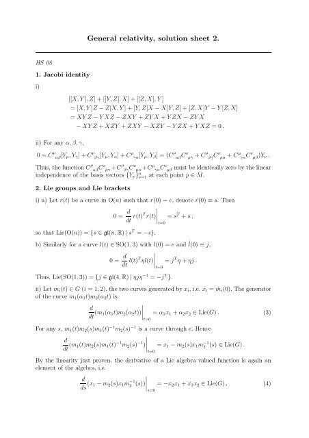
General relativity, solution sheet 2.

General relativity, solution sheet 2.
HS 08
1. Jacobi identity
i)
ii) For any α, β, γ,
[[X, Y ], Z] + [[Y, Z], X] + [[Z, X], Y ]
= [X, Y ]Z − Z[X, Y ] + [Y, Z]X − X[Y, Z] + [Z, X]Y − Y [Z, X]
= XY Z − Y XZ − ZXY + ZY X + Y ZX − ZY X
− XY Z + XZY + ZXY − XZY − Y ZX + Y XZ = 0 .
0 = C µ αβ [Y µ, Y γ ] + C µ βγ [Y µ, Y α ] + C µ γα [Y µ, Y β ] = (C µ αβ Cν µγ + Cµ βγ Cν µα + Cµ γα Cν µβ )Y ν .
Thus, the function C µ αβ Cν µγ +C µ βγ Cν µα+C µ γαC ν µβ must be identically zero by the linear
independence of the basis vectors {Y ν } n ν=1 at each point p ∈ M.
2. Lie groups and Lie brackets
i) a) Let r(t) be a curve in O(n) such that r(0) = e, denote ṙ(0) ≡ s. Then
0 = d dt r(t)T r(t)
∣ = s T + s ,
t=0
so that Lie(O(n)) = {s ∈ gl(n, R) | s T = −s}.
b) Similarly for a curve l(t) ∈ SO(1, 3) with l(0) = e and ˙l(0) ≡ j,
0 = d dt l(t)T ηl(t)
∣ = j T η + ηj .
t=0
Thus, Lie(SO(1, 3)) = {j ∈ gl(4, R) | ηjη −1 = −j T }.
ii) Let m i (t) ∈ G (i = 1, 2), the two curves generated by x i , i.e. x i = ṁ i (0). The generator
of the curve m 1 (α 1 t)m 2 (α 2 t) is
d
dt (m 1(α 1 t)m 2 (α 2 t))
∣ = α 1 x 1 + α 2 x 2 ∈ Lie(G) . (3)
t=0
For any s, m 1 (t)m 2 (s)m 1 (t) −1 m 2 (s) −1 is a curve through e. Hence
d
dt (m 1(t)m 2 (s)m 1 (t) −1 m 2 (s) −1 )
∣ = x 1 − m 2 (s)x 1 m −1
2 (s) ∈ Lie(G) .
t=0
By the linearity just proven, the derivative of a Lie algebra valued function is again an
element of the algebra, i.e.
d
ds (x 1 − m 2 (s)x 1 m −1
2 (s)) ∣
∣∣∣s=0
= −x 2 x 1 + x 1 x 2 ∈ Lie(G) . (4)

Finally, (4) follows from (2,3) and the distributivity for n × n matrices.
iii) It follows from ϕ ∗ [X, Y ] = [ϕ ∗ X, ϕ ∗ Y ], see lecture notes p.7, that
(λ g ) ∗ [X, Y ] = [X, Y ]
for any two left-invariant vector fields X, Y .
iv) Applying (λ g ) ∗ to (1) gives
[Y α , Y β ] = (λ g ) ∗ (C γ αβ Y γ) = (C γ αβ ◦ λ g)Y γ .
Comparison with (1) yields, by the independence of the Y γ , C γ αβ ◦ λ g
C γ αβ (gh) = Cγ αβ (h). Hence Cγ αβ
is constant.
= C γ αβ , i.e.
v) Left-invariance means X gh = (λ g ) ∗ X h . For h = e this shows that X e ∈ T e (G) = Lie(G)
determines X g at all g ∈ G.
vi) Let us first recall that the relation X ↔ x between the (abstract) left-invariant vector
field X and its matrix form x is
(Xf)(e) = d dt f(m(t)) ∣
∣∣∣t=0
, (f ∈ F(G)) ,
where ṁ(0) = x. Hence α 1 x 1 + α 2 x 2 corresponds to (see (3))
d
dt f(m 1(α 1 t)m 2 (α 2 t))
∣ = d t=0
dt f(m 1(α 1 t))
∣ + d t=0
dt f(m 2(α 2 t)) ∣
= α 1 (X 1 f)(e) + α 2 (X 2 f)(e) ,
by using the chain rule, i.e., to α 1 X 1 + α 2 X 2 . To establish the second correspondence
consider the conjugation τ h : G → G, g ↦→ hgh −1 . One verifies λ g ◦ τ h = τ h ◦ λ h −1 gh,
implying (λ g ) ∗ (τ h ) ∗ = (τ h ) ∗ (λ h −1 gh) ∗ . Hence (τ h∗ )X is left-invariant if X is; moreover
(τ h∗ )X ↔ hxh −1 because
d
dt f(hm(t)h−1 )
∣ = d t=0
dt (f ◦ τ h)(m(t))
∣ = (τ h∗ Xf)(e) (5)
t=0
by the definition of the tangent map. In particular
(τ m2 (s)) ∗ X 1 ←→ m 2 (s)x 1 m 2 (s) −1
and by the already established linearity of the correspondence it extends to the derivative
w.r.t. s. On the l.h.s we have by (5)
d
ds τ m 2 (s)∗X 1 f(e)
∣ = d d
s=0
ds dt f(m 2(s)m 1 (t)m 2 (s) −1 )
∣
s=t=0
= d d f(m2 (s)m 1 (t)) + f(m 1 (t)m 2 (s)
ds dt( −1 ) )∣ ∣∣s=t=0
= d ds X 1(f ◦ λ m2 (s))(e)
∣ − d s=0
dt X 2(f ◦ λ m1 (t))(e) ∣
= ((X 1 X 2 − X 2 X 1 )f)(e) ,
∣
t=0
∣
t=0

i.e.
On the r.h.s. we have, see (4)
d
ds τ m(s)∗X 1
∣
∣∣∣s=0
= [X 1 , X 2 ] .
d
ds m 2(s)x 1 m 2 (s) −1 ∣
∣∣∣s=0
= [x 1 , x 2 ] .