Exercise 10 (PDF, 127 kB)
Exercise 10 (PDF, 127 kB)
Exercise 10 (PDF, 127 kB)

Create successful ePaper yourself
Turn your PDF publications into a flip-book with our unique Google optimized e-Paper software.
Statistical Physics<br />
<strong>Exercise</strong> <strong>10</strong><br />
HS 12<br />
Prof. M. Sigrist<br />
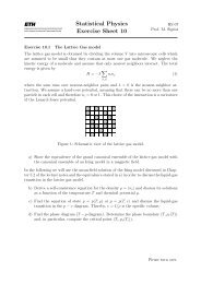
<strong>Exercise</strong> <strong>10</strong>.1<br />
Bose–Einstein Condensation<br />
a) In Section 4.5 of the lecture notes, we have derived an expression for the specific<br />
heat C V (T ) of the spinless Bose gas both above and below the critical temperature<br />
T c (Eq. 4.81). While C V does not diverge at T c , it has a cusp there (Fig. 4.4),<br />
suggesting that a T -derivative of C V does diverge.<br />
Evaluate<br />
∆ =<br />
lim ∂ T C V (T ) − lim ∂ T C V (T ) ≠ 0<br />
T →T c+ T →T c−<br />
to show that ∂ T C V (T ) is not continuous at T c , and conclude that indeed ∂ 2 T C V (T )<br />
diverges at the critical temperature.<br />
b) As we saw in a), in the vicinity of a phase transition several thermodynamic quantities<br />
may show non-analytic behavior. The way in which these quantities diverge<br />
gives us useful information about the transition itself. Oftentimes, one finds that<br />
some quantity X shows a power-law behavior near the critical temperature, i.e.,<br />
X(T ) ∝ (T − T c ) γ . The exponent γ is called the corresponding critical exponent.<br />
Show that the compressibility κ T of the spinless Bose gas satisfies a power law for<br />
T → T c +, and find the corresponding critical exponent.<br />
Hint: At T = T c we have z = 1. It is convenient to expand κ T<br />
ν = ln z about ν = 0.<br />
<strong>Exercise</strong> <strong>10</strong>.2<br />
Magnetostriction in a Spin-Dimer-Model<br />
in the variable<br />
As in <strong>Exercise</strong> 8.2, we consider a dimer consisting of two spin-1/2 particles with Hamilton<br />
operator<br />
(<br />
H 0 = J ⃗S1 · ⃗S<br />
)<br />
2 + 3/4<br />
and J > 0 (note that the energy levels are shifted as compared to Ex. 8.2). This time,<br />
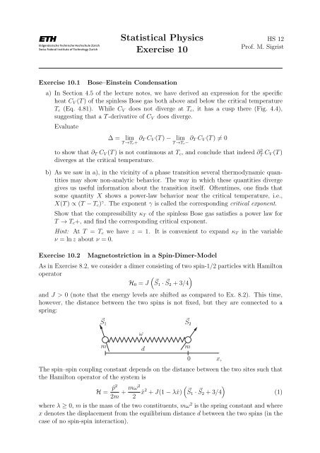
however, the distance between the two spins is not fixed, but they are connected to a<br />
spring:<br />
⃗S 1 S2 ⃗<br />
ω<br />
m<br />
d<br />
m<br />
0 x,<br />
The spin–spin coupling constant depends on the distance between the two sites such that<br />
the Hamilton operator of the system is<br />
(<br />
H = ˆp2<br />
2m + mω2<br />
2 ˆx2 + J(1 − λˆx) ⃗S1 · ⃗S 2 + 3/4)<br />
(1)<br />
where λ ≥ 0, m is the mass of the two constituents, mω 2 is the spring constant and where<br />
x denotes the displacement from the equilibrium distance d between the two spins (in the<br />
case of no spin-spin interaction).
a) Write the Hamiltonian (1) in second quantized form and calculate the partition sum,<br />
the internal energy, the specific heat and the entropy. Discuss the behavior of the<br />
entropy in the limit T → 0 for different values of λ.<br />
Hint: Set = 1 and introduce an observable ˆn t satisfying<br />
{<br />
1 if σ is a triplet<br />
〈σ|ˆn t |σ〉 =<br />
0 if σ is a singlet<br />
for any vector |σ〉 in the Hilbert space describing the spin part of the dimer.<br />
b) Calculate the expectation value of the distance of the two spins, 〈d + ˆx〉, as well as<br />
the fluctuation, 〈(d + ˆx) 2 〉. How are these quantities affected by a magnetic field in<br />
z-direction, i.e., by adding an additional term in (1) of the form<br />
H m = −gµ B H ∑ i<br />
S z i ?<br />
c) If the two sites are oppositely charged, i.e., ±q, the dimer forms a dipole with<br />
moment P = q〈d+x〉. This dipole moment can be measured by applying an electric<br />
field E in x-direction,<br />
H el = −q(d + ˆx)E.<br />
Calculate the zero-field susceptibility of the dimer,<br />
χ (el)<br />
0 = − ∂2 F<br />
∂E 2 ∣<br />
∣∣∣E=0<br />
,<br />
and compare your result with the fluctuation-dissipation theorem which asserts that<br />
χ (el)<br />
0 ∝ 〈 (d + ˆx) 2〉 − 〈 d + ˆx 〉 2<br />
.<br />
Plot the zero-field susceptibility as a function of the applied magnetic field H and<br />
discuss your result.<br />
Office Hours: Monday, November 26th, 8–<strong>10</strong> AM (Michael Walter, HIT K 31.5)