Statistical Physics Exercise Sheet 10

Statistical Physics
Exercise Sheet 10
HS 07
Prof. M. Sigrist
Exercise 10.1
The Lattice Gas model
The lattice gas model is obtained by dividing the volume V into microscopic cells which
are assumed to be small that they contain at most one gas molecule. We neglect the
kinetic energy of a molecule and assume that only nearest neighbors interact. The total
energy is given by
H = −λ ∑ 〈i,j〉
n i n j (1)
where the sum runs over nearest-neighbor pairs and λ > 0 is the nearest-neighbor attraction.
We assume a hard-core potential, meaning that there can be no more than one
particle in each cell and therefore n i = 0 or 1. This choice of the interaction is a caricature
of the Lenard-Jones potential.
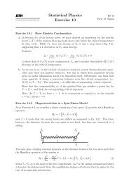
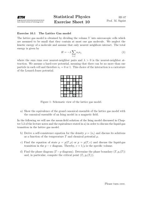
Figure 1: Schematic view of the lattice gas model.
a) Show the equivalence of the grand canonical ensemble of the lattice gas model with
the canonical ensemble of an Ising model in a magnetic field.
In the following we will use the mean-field solution of the Ising model discussed in Chapter
5.2 of the lecture notes and the equivalence stated in a) in order to discuss the liquid-gas
transition in the lattice gas model.
b) Derive a self-consistence equation for the density ρ = 〈n i 〉 and discuss its solutions
as a function of the temperature T and chemical potential µ.
c) Find the equation of state p = p(T, ρ) or p = p(T, v) and discuss the liquid-gas
transition in the p − v diagram. Thereby, v = 1/ρ is the specific volume.
d) Find the phase diagram (T − p diagram). Determine the phase boundary (T, p c (T ))
and, in particular, compute the critical point (T c , p c (T c )).
Please turn over.

Exercise 10.2
Magnetic domain wall
We want to calculate the energy of a magnetic domain wall in the framework of the
Ginzburg-Landau (GL) theory. We assume translational symmetry in the (y, z)-plane in
which case the GL functional in zero field reads
∫ { A
F [m, m ′ ] = F 0 + dx
2 m(x)2 + B 4 m(x)4 + κ }
2 [m′ (x)] 2 . (2)
a) Solve the GL equation with boundary conditions
m(x → ±∞) = ±m 0 , m ′ (x → ±∞) = 0. (3)
Here, m 0 is the magnetization of the uniform solution.
b) Compute the energy of the solution in a) as compared to the uniformly polarized
solution. Use the coefficients A and B according to the expansion of the mean-field
free energy of the Ising model [see Eq. (5.64)]. Compare the energy of the domain
wall with the energy of a sharp step in the magnetization.