Solid State Theory Solution Sheet 5

Solid State Theory
Solution Sheet 5
FS 13
Prof. M. Sigrist
Exercise 5.1
Coulomb interaction - excitons
We want to study the influence of the electron-electron interaction on the excitation
spectrum of the half-filled chain.
1. In the following we show that the repulsive interaction between the electrons leads
to an attractive interaction between the electrons in the conduction band and the
holes in the valence band.
We consider the following repulsive interaction:
Û = U
N/2
N∑
∑
n i n i+1 = U n 2i (n 2i−1 + n 2i+1 ). (1)
i=1
i=1
We want to find a simple expression in terms of the operators a k and b k . We start
with the density operator n j = c † j c j.
n 2j = 1 ∑∑
e i(k−k′ )2j c † k
N
c k ′
k k ′
= 1 ∑′∑′ e
i(k−k ′)2j (c † k
N
c k ′ + c† k c k ′ +π + c † k+π c k ′ + c† k+π c k ′ +π)
k k ′
= 1 ∑′∑′ e
i(k−k ′)2j (c † k
N
+ c† k+π ) (c k ′ + c
} {{ } } {{ k ′ +π)
}
k k ′ ≈− √ 2b † ≈− √ 2b
k
k ′
≈
2 ∑′∑′ e
i(k−k ′)2j b † k
N
b k ′. (2)
k k ′
Here, we used that u ±π/2 = −v ±π/2 = 1/ √ 2, and where the ∑′ runs over the reduced
Brillouin zone. Note that the above approximation is only valid in the vicinity of
k = ±π/2. However, for u ≪ v, t this is the region which is most affected by the
interaction and the approximation is justified in this limit. In a similar way one
shows
n 2j±1 ≈ 2 ∑′∑′ e
i(k−k ′)(2j±1) a † k
N
a k ′. (3)
k k ′
In the vicinity of the band gap, namely for k ≈ ±π/2, the ’a-particles’ live solely
on the odd lattice sites whereas the ’b-particles’ are exclusively on the even lattice
sites. In other words, the electrons near the Fermi surface (for U = 0) have optimally
arranged themselves to gain as much energy as possible from the potential ˆV . This
means that if an electron-hole pair is created we find that the electron will mainly
be on the even sites while the hole will be on the odd sites. This is in fact the
reason why we need a non-local interaction between the electrons (as modeled by
Û) in order to have an attractive interaction between holes and electrons. A local
interaction (which anyway is not possible for spinless fermions) would not be able
to do this job.
1

Using Eqs. (2), (3) and (1) we obtain
Û ≈ 4U
≈
∑
′ N/2
N 2
k 1 ,...,k 4 j=0
4U
N
∑
With the substitution
∑
e i(k 1−k 2 +k 3 −k 4 )2j (e i(k 3−k 4 ) + e −i(k 3−k 4 ) )b † k 1
b k2 a † k 3
a k4 (4)
k 1 ,...,k 4
′
δk1 +k 3 ,k 2 +k 4
cos(k 3 − k 4 )b † k 1
b k2 a † k 3
a k4 . (5)
k 1 → k k 2 → k ′ k 3 → k ′ + q k 4 → k + q (6)
the constraint k 1 + k 3 = k 2 + k 4 is automatically fulfilled and we obtain
Û ≈ − 4U N
∑
k,k ′ ,q
′
cos(k − k ′ )a k+q b † k b k ′a† k ′ +q
+ 4U ∑ b †
✟ ✟✟✟✟✟ k b k
(7)
k
as on the exercise sheet. The minus sign in the above equation stems from the
exchange of the fermionic operator a † k ′ +q
with three fermionic operators. This minus
sign is very important since it yields an attraction between electrons and holes. In
addition, in Eq. (7) we dropped a term proportional to the total number of electrons
in the conduction band which is irrelevant for the following discussion.
2. The Hamilton operator H = H 1 + Û with the approximation (7) for Û separately
preserves the number of electrons and holes and therefore we can use the following
ansatz for the wave function of the exciton:
|ψ q 〉 = ∑ k
′
A
q
k a k+qb † k
|Ω〉. (8)
Note that this ansatz yields exact eigenstates of H only in the case when Û is
approximated according to Eq. (7). The exact Û does not preserve the number of
electrons and holes separately and leads to a complicated many-body problem.
The coefficients A q k and the excitation energy ω q of the exciton have to be determined
such that
( ˜H 1 + Û)|ψ q〉 = ω q |ψ q 〉 (9)
where ˜H 1 = H 1 −E 0 , meaning that energies are measured with respect to the ground
state energy E 0 . For this we need the action of Û on an exciton state,
and the action of ˜H 1 ,
Û|ψ q 〉 = − 4U N
∑′∑
k ′
k ′′ ′
A
q
k ′ cos(k ′ − k ′′ )a k ′′ +qb † k ′′ |Ω〉, (10)
˜H 1 |ψ q 〉 = ∑ k
′
A
q
k (E k + E k+q )a k+q b † k
|Ω〉. (11)
Consequently, the Eq.(9) written component by component has to hold
(E k + E k+q − ω q )A q k = 4U N
2
∑
k ′
′
A
q
k ′ cos(k ′ − k) (12)

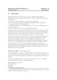
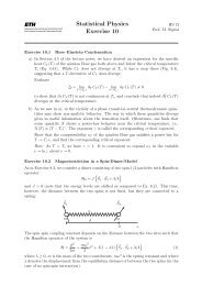
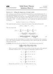
Figure 1: Graphical solution of Eq. (16), for q = 0, V/t = 1 and N = 8 (left) and
N = 20 (right). We are looking for solutions with energy smaller than the band gap
(indicated by dashed line in left plot), such that ω q=0 < 2V . The plots show that a
solution exists for each such ω q=0 . The sum in Eq. 16 has a divergent term for each k
(when ω q=0 = 2E k , corresponding to a particle-hole excitation energy), and so we expect
as many divergencies as there are k values. This is illustrated by the two different plots
for N = 8 and for N = 20, which due to their different lengths have a different number of
allowed (discrete) k values. Notice also that if the energy of the exciton becomes larger
than the difference between the valence band bottom and conduction band top, there are
no more particle-hole excitations.
We assume that U ≪ V, t. In this case the bound state will be strongly extended in
real space, meaning that A q k
is localized in k-space. Therefore, in Eq. (12) we can
put the cos-factor out of the sum and approximate it by 1. 1 Then, dividing both
sides by (E k + E k+q − ω q ) and summing over k yields
1
4U = 1 N
∑
k
′ 1
E k + E k+q − ω q
. (16)
The solutions of this equation for q = 0 for a small chain (N = 8) and a larger chain
(N = 20) are shown in Fig. 1. Note that there is an exciton excitation with energy
smaller than the gap ∆ = 2V . Now we have revealed a bound state called exciton.
3. In the following we want to calculate the energy dispersion ω q of the excitons for
1 The proper way how to solve the Eq. (12) is to use
cos(k − k ′ ) = cos k cos k ′ − sin k sin k ′ , (13)
and write down two self-consistent equations for F q 1 ≡ ∑ ′
k ′ Aq k
cos k ′ and F q ′ 2 ≡ ∑ ′
k ′ Aq k
sin k ′ by dividing
′
Eq. (12) by (E k + E k+q − ω q ), multiplying by cos k (or sin k) and subsequent summation over k:
F q 1 = 4U ∑′ F q 1 cos2 k + F q 2 cos k sin k
, (14)
N E k + E k+q − ω q
F q 2 = 4U N
k
∑
k
′ F q 1 cos k sin k + F q 2 sin2 k
E k + E k+q − ω q
, (15)
and the non-trivial solution of this homogeneous set of equations exist only if the determinant vanishes...
As you see the approximation greatly simplifies the further analysis.
3

small q. For this we write the sum as an integral
1
4U = I := 1 1
2 N/2
′∑ 1
= 1 1
E k + E k+q − ω q 2 π
k
∫ π/2
−π/2
dk
E k + E k+q − ω q
. (17)
For small u the integral has to become large. Since the exciton energy lies within
the gap the main contributions to the integral are from the vicinity of k = ±π/2.
We therefore expand the denominator around k = ±π/2 and for small q’s:
E k + E k+q ≈ 2V + 2t2
V
((k ∓ π 2 )2 + (k + q ∓ π 2 )2 )
} {{ }
2(k ∓ π 2 + q 2 )2 + q2
2
So the denominator has minima 2V + t 2 q 2 /V at k = ±π/2 − q/2. For small U, ω q
is only little less then the minimum and almost all the contributions come from the
vicinity of the minimum. Therefore, we introduce a cutoff Λ and write the integral
symmetrically around 0,
(18)
I ≈ 1 ∫ Λ
2π −Λ
dk
2V + t2 q 2
− ω
V q + 4t2 k 2
V
= 1
√ ∫ V
˜Λ
dx
2π 4t 2 −˜Λ a 2 + x , (19)
2
where we have defined a 2 = 2V − ω q + t 2 q 2 /V . Finally, we obtain
I ≈ 1
√
V 1
( x
)∣
√
∣∣˜Λ V
2π 4t 2 a arctan 1
≈
a −˜Λ 4t 2 2a . (20)
Here we let the cutoff to infinity. Solution ω q of Eq. (17) yields the dispersion
ω q = 2V − U 2 V
t 2
+ t2
V q2 = 2V − U 2 V
t 2 + q2
2(2m ∗ )
(21)
where m ∗ = V/(4t 2 ) is the effective mass near the energy gap. Thus, the electronhole
pair has twice the mass of a single electron or hole.
4. To show how f(r − r ′ ) is related to A 0 k , we insert the Fourier expansion of
a k
= 1 ∫ L
dre ikr a (r) , b † k
2L
= 1 ∫ L
dr ′ e −ikr′ b † (r ′ ) , (22)
−L
2L −L
into the continuous form of the exciton state (for now considering finite volume,
thus k = nπ/L),
|ψ q=0 〉 = ∑ k
A 0 ka k
b † k |Ω〉 = 1 ∫ L
dx dx ′ 1 ∑
A 0
2L −L 2L
ke ik(r−r′ )
k
} {{ }
f(r−r ′ )
a (r)b † (r ′ ) . (23)
Now we do a limit L → ∞ to conclude that
f(ρ) = 1 ∫
dkA 0
2π
ke ikρ . (24)
R
4

In order to evaluate f(ρ), we use eq. (12) (note that the right-hand-side is a constant),
so that A 0 k ∝ (2E k − ω 0 ) −1 ; plugging into Eq. (24) yields to
∫ ∞
f(ρ) ∝ m ∗ e ikρ
dk
k 2 + m ∗ (2V − ω 0 ) ; 2V − ω 0 > 0 ; (25)
−∞
which can be evaluated using the method of residues. Note that f(ρ) is real due to
antisymmetry of the imaginary part of the integral. Moreover, f(ρ) is symmetric, as
f(−ρ) = f(ρ) ∗ = f(ρ). For ρ > 0, the contour may be closed in the upper half of the
complex plane where there is a single simple pole located at ˜k = i √ m ∗ (2V − ω 0 ),
so that λ = [m ∗ (2V − ω 0 )] −1/2 .
Exercise 5.2
Graphene
f(ρ) ∝ m ∗ (2πi) ei˜k|ρ|
2˜k ∝ e−|ρ|√ m ∗ (2V −ω 0 ) , (26)
We want to calculate the π-energy bands of graphene using the tight-binding method.
Those bonds are due to electrons in the 2p z orbitals. Graphene has two inequivalent
carbon atoms per unit cell, which we call A and B.
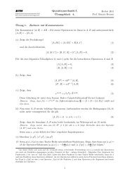
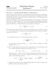
The primitive lattice vectors ⃗a i join atoms on the same sublattice (A or B), so that the
reference points of the unit cells (the A-atoms in Fig. 2) form a triangular lattice. Setting
the lattice constant a to unity they are given by
(√ )
3
⃗a 1 =
2 , 1 2
(√ )
3
⃗a 2 =
2 , −1 . (27)
2
The reciprocal lattice vectors ⃗c i can be found as usually by demanding that they satisfy
⃗c i · ⃗a j = 2πδ ij . (28)
This leads to
(
⃗c 1 = √ 4π
√ )
1 3
3 2 , 2
( )
⃗c 2 = √ 4π 1
3 2 , −√ 3
2
(29)
With the reciprocal lattice vectors the Brillouin zone can be constructed and is seen to be
a regular hexagon (Fig. 2). Note that after identifying points that differ by a reciprocal
lattice vector only two of the corners are inequivalent.
Next we find the general form of the tight-binding model for the bands originating in the
p z -orbitals when only nearest neighbor hopping is taken into account. The p z -orbitals are
symmetric under the rotations of the plane so that the hopping matrix elements do not
depend on the direction. Hence we have only one hopping parameter, which we denote
5

2
3
A
b 1
B
y
x
a 1
a 2
Γ
c
K
M
k x
k y
c
Figure 2: Left: Primitive lattice vectors for the honeycomb lattice. The vectors join points
on one triangular sublattice. Right: Hexagonal Brillouin zone constructed from the reciprocal
lattice vectors ⃗c 1 and ⃗c 2 .
by t. Furthermore, every A-atom has neighbors in B only. The onsite terms have to be
the same on both sublattices, so that they can be absorbed into the chemical potential
(we work at fixed filling with two electrons per unit cell).
To describe the hopping terms we define the vectors
( )
⃗ 1
b1 = √3 , 0 ,
(
⃗ −1
b2 =
2 √ 3 , 1 )
, and
2
(
⃗ −1
b3 =
2 √ 3 , −1 )
(30)
2
that point from an A atom to its three nearest neighbors. Denoting the postion of the
i-th atom on sublattice A by ⃗ R a,i , the Hamiltonian is given by
H = t ∑ i
3∑
j=1
( ) ( [c † ⃗Ra,i c ⃗Ra,i + ⃗ ) ]
b j + h.c. . (31)
Now we use the Fourier transform given on the exercise sheet,
( )
c ⃗Ra,i
1 ∑
= √
N
to find
H = t N
= t ∑ k∈BZ
( )
c ⃗Rb,i
∑
k,k ′ ∈BZ
(
ã†
k
˜b†
k
ã † k˜b k ′
=
∑
i
) ( 0
1 ∑
√
N
⃗ k∈BZ
ã k e i⃗ k· ⃗R a,i
⃗ k∈BZ
˜bk e i⃗ k· ⃗R b,i
, (32)
e i ⃗ R a,i (k ′ −k)
3∑
e i⃗ k ′·⃗b j
+ h.c.
j=1
∑
j ei⃗ k·⃗b j
∑
j e−i⃗ k·⃗b j
0
6
) (
ãk
˜bk
)
. (33)

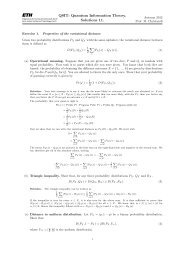
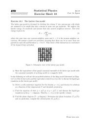
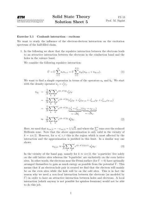
Figure 3: left: Dispersion of the two bands of graphene. At half-filling (one electron per p z -
orbital), the Fermi ’surface’ consists of two points at the two inequivalent corners of the Brillouin
zone. right: Dirac cone in the vicinity of the point ⃗ k = (2π/ √ 3, 2π/3)
The dispersion is found by diagonalizing the 2 × 2-matrix Hamiltonian which yields
(√ )
ɛ k = ± t √ 3
3 + 4 cos
2 k x cos k y
2 + 2 cos k y. (34)
The two bands are shown in figure 3. With two electrons per unit cell the lower band is
completely filled whereas the upper band is empty, so that µ = 0.
Now we can find the position of the Fermi points displayed in figure 3 by solving
3∑
e i⃗ k·⃗b j
= 0. (35)
j=1
Inserting the definition of ⃗ b j in (30) and writing equations for the real and imaginary
parts separately we have
( ) ( )
qx
qx
(
cos √ + 2 cos 3 2 √ qy
)
cos = 0 and (36)
3 2
( ) ( )
kx
qx
sin √ − 2 sin 3 2 √ cos( k y
) = 0, (37)
3 2
which has as solutions ⃗q 1 =
( )
√2π
3
, 2π and ⃗q
3
2 = ( )
0, 4π 3 , i.e. the two inequivalent corners of
the Brillouin zone. Note that both bands touch at these points. Next we obtain the low
energy Hamiltonian by expanding (33) to linear order around the corners of the Brillouin
zone, so that
H eff ≈ − 3√ 3t
8π
∑
k
2∑
i=1
(
Ψ † i (⃗ k) ˆσ x ⃗q i · ⃗k + ˆσ y (ˆɛ⃗q i ) · ⃗k
)
Ψ i ( ⃗ k), (38)
where ˆɛ is the antisymmetric tensor and σ i are the Pauli matrices. The effect of the
ansisymmetric tensor is as follows when summing over i: if i = 1 we have q 1 in the first
term and −q 2 in the second (and vice versa). The Ψ i describe the electrons at the Fermi
point q i , and have two components for each i describing the upper and the lower band.
7

The momenta ⃗ k are relative to the Fermi points (i.e. shifted by ⃗q i ). The corresponding
low energy dispersion is E = ±v F |k|, which resembles the relativistic energy-momentum
relation E 2 = m 0 c 4 + p 2 c 2 for a massless particle and the speed of light replaced by the
Fermi velocity. In fact, (38) is equivalent to the Dirac equation in (2 + 1)-dimensional
spacetime. The Fermi sea below each Fermi point corresponds to the Dirac sea (vacuum
for anti-particles), and the two Fermi points correspond to the two different chiralities of
spin-1/2 particles in relativistic QFT. This fact allows studying some of the more puzzling
aspects of the Dirac equation (such as the Klein paradox, see e.g. M. I. Katsnelson et al.,
Chiral tunnelling and the Klein paradox in graphene, Nature Physics 2, 620 - 625 (2006)).
8