Wave Synchronizing Crane Control during Water Entry in ... - NTNU
Wave Synchronizing Crane Control during Water Entry in ... - NTNU
Wave Synchronizing Crane Control during Water Entry in ... - NTNU

Create successful ePaper yourself
Turn your PDF publications into a flip-book with our unique Google optimized e-Paper software.
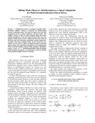
<strong>Wave</strong> <strong>Synchroniz<strong>in</strong>g</strong> <strong>Crane</strong> <strong>Control</strong> <strong>dur<strong>in</strong>g</strong> <strong>Water</strong> <strong>Entry</strong> <strong>in</strong> Offshore<br />
Moonpool Operations – Experimental Results<br />
Tor A. Johansen 1 , Thor I. Fossen 1 , Sve<strong>in</strong> I. Sagatun 2 , and F<strong>in</strong>n G. Nielsen 2<br />
Abstract<br />
A new strategy for active control <strong>in</strong> heavy-lift offshore crane<br />
operations is suggested, by <strong>in</strong>troduc<strong>in</strong>g a new concept referred<br />
to as wave synchronization. <strong>Wave</strong> synchronization<br />
reduces the hydrodynamic forces by m<strong>in</strong>imization of variations<br />
<strong>in</strong> the relative vertical velocity between payload and<br />
water us<strong>in</strong>g a wave amplitude measurement. <strong>Wave</strong> synchronization<br />
is comb<strong>in</strong>ed with conventional heave compensation<br />
to obta<strong>in</strong> accurate control. Experimental results us<strong>in</strong>g a scale<br />
model of a semi-submerged vessel with a moonpool shows<br />
that wave synchronization leads to significant improvements<br />
<strong>in</strong> performance. Depend<strong>in</strong>g on the sea state and payload, the<br />
results <strong>in</strong>dicate that the reduction <strong>in</strong> the standard deviation of<br />
the wire tension may be up to 50 %.<br />
1 Introduction<br />
Higher operability of <strong>in</strong>stallations offshore of underwater<br />
equipment will become <strong>in</strong>creas<strong>in</strong>gly more important <strong>in</strong> the<br />
years to come. Offshore oil and gas fields will be developed<br />
1 Department of Eng<strong>in</strong>eer<strong>in</strong>g Cybernetics, Norwegian University<br />
of Science and Technology, N-7491, Trondheim, Norway.<br />
Tor.Arne.Johansen@itk.ntnu.no, tif@itk.ntnu.no<br />
2 Norsk Hydro Exploration and Production, Bergen,<br />
Norway.<br />
Sve<strong>in</strong>.Ivar.Sagatun@hydro.com,<br />
F<strong>in</strong>n.Gunnar.Nielsen@hydro.com<br />
with all process<strong>in</strong>g equipment on the seabed and <strong>in</strong> the production<br />
well itself. Norsk Hydro has already one year of operational<br />
experience with the Troll Pilot subsea oil process<strong>in</strong>g<br />
plant. This subsea plant is made up of a three phase subsea<br />
separator, a 1.6 MW electrical s<strong>in</strong>gle phase pump and a re<strong>in</strong>jection<br />
tree; everyth<strong>in</strong>g located on 320 m water depth outside<br />
the west coast of Norway. Process equipment like subsea<br />
electrical multi phase pumps, subsea and down hole separators,<br />
frequency converters, electrical distribution, manifolds,<br />
control and <strong>in</strong>strumentation systems are all process system<br />
components which are ready for use <strong>in</strong> subsea production.<br />
The lower cost <strong>in</strong> us<strong>in</strong>g subsea equipment compared to us<strong>in</strong>g<br />
a float<strong>in</strong>g or fixed production platform is penalized with<br />
lower availability for ma<strong>in</strong>tenance, repair and replacement<br />
of equipment. Production stops due to component failure is<br />
costly, hence a high operability on subsea <strong>in</strong>tervention is required<br />
to operate subsea fields. High operability implies that<br />
subsea <strong>in</strong>tervention must be carried out also <strong>dur<strong>in</strong>g</strong> w<strong>in</strong>ter<br />
time, which <strong>in</strong> the North Sea and other exposed areas implies<br />
underwater <strong>in</strong>tervention <strong>in</strong> harsh weather conditions.<br />
Standard <strong>in</strong>dustrial heave compensation systems applied to<br />
offshore cranes or module handl<strong>in</strong>g systems (MHS) have<br />
been used by the <strong>in</strong>dustry for years, see for <strong>in</strong>stance [1, 2,<br />
3, 4, 5] and references there<strong>in</strong>. These systems normally work<br />
p. 1
with acceleration feedback or feedforward, where the vertical<br />
acceleration is measured on the vessel, on the crane boom,<br />
or MHS structure.<br />
Alternatively, a passive spr<strong>in</strong>g-damper<br />
mechanism together with position control of the crane hook<br />
is used for heave compensation <strong>dur<strong>in</strong>g</strong> the water entry phase.<br />
This article focuses on active control of heave compensated<br />
cranes or MHS <strong>dur<strong>in</strong>g</strong> the water entry phase of a subsea<br />
<strong>in</strong>stallation or <strong>in</strong>tervention. We assume that the payload is<br />
launched through a moonpool from a typical mono hull <strong>in</strong>stallation<br />
vessel, see Fig 1. Dur<strong>in</strong>g the water entry phase the<br />
hydrodynamic loads due to waves with<strong>in</strong> the moonpool may<br />
be significant, and not directly accounted for <strong>in</strong> a heave compensation<br />
system. The ma<strong>in</strong> contribution of the present work<br />
is the use of moonpool wave amplitude feedforward control<br />
<strong>in</strong> order to achieve wave synchronized motion of the payload<br />
through the water entry zone. We believe this concept is new.<br />
The paper is organized as follows: In Section 2 we describe<br />
a mathematical model of a 1:30 scale model semi-submerged<br />
vessel with moonpool and crane/payload. A frequency analysis<br />
of the crane system is given <strong>in</strong> Section 3. Based on this<br />
model and analysis, a wave synchroniz<strong>in</strong>g control strategy is<br />
derived <strong>in</strong> Section 4, and experimentally verified us<strong>in</strong>g the<br />
scale model <strong>in</strong> the Mar<strong>in</strong>e Cybernetics laboratory (MCLab<br />
[6]), as described <strong>in</strong> Section 5. Some conclusions are presented<br />
<strong>in</strong> Section 6. A short prelim<strong>in</strong>ary version of this paper<br />
is [7].<br />
Figure 1: An example of multipurpose <strong>in</strong>tervention vessel<br />
equipped with a moonpool and a MHS.<br />
vessel. It is assumed that the vessel is kept <strong>in</strong> a mean fixed<br />
position and head<strong>in</strong>g relative to the <strong>in</strong>com<strong>in</strong>g wave. Effects<br />
from the vessel’s roll and pitch motion are neglected.<br />
2.1 Dynamics of scale model crane-vessel<br />
In this section we describe the rigid-body dynamics of a laboratory<br />
scale model moonpool crane-vessel (scale 1:30), see<br />
Figures 2 and 3 of a setup consist<strong>in</strong>g of an electric motor<br />
and a payload connected by a wire that runs over a pulley<br />
suspended <strong>in</strong> a spr<strong>in</strong>g. The spr<strong>in</strong>g is designed to simulate a<br />
realistic wire elasticity <strong>in</strong> the scale model. We remark that<br />
this setup conta<strong>in</strong>s no passive heave compensation system.<br />
The equations of motion for the motor and payload are<br />
2 Mathematical modell<strong>in</strong>g<br />
We will only consider the vertical motion of a payload mov<strong>in</strong>g<br />
through the water entry zone, handled from a float<strong>in</strong>g<br />
m m ¨z m F m · F t (1)<br />
m´¨z · ¨z 0<br />
µ mg · f z F t (2)<br />
where z m Rθ m , m m J m R, F m T m R, and<br />
p. 2
Figure 2: Rig-crane scale model.<br />
Figure 3: Def<strong>in</strong>ition of the coord<strong>in</strong>ate systems.<br />
θ m motor angle (rad)<br />
R radius of the pulley on the motor shaft (m)<br />
J m motor <strong>in</strong>ertia (kgm)<br />
T m motor torque (Nm)<br />
m payload mass (kg)<br />
z 0 vessel position <strong>in</strong> heave (m)<br />
z payload position (m)<br />
z m motor position (m)<br />
ζ wave amplitude at center of moonpool (m)<br />
F t wire tension (N)<br />
f z hydrodynamic and static force on payload (N)<br />
All coord<strong>in</strong>ate systems and forces are positive downwards.<br />
The coord<strong>in</strong>ate systems of zz m and z p are fixed <strong>in</strong> the vessel,<br />
while the coord<strong>in</strong>ate systems of ζ and z 0<br />
are Earth-fixed, see<br />
Figure 3. All have the orig<strong>in</strong> at the still water mean sea level.<br />
The wire runs over a pulley suspended <strong>in</strong> a spr<strong>in</strong>g. The mass<br />
mov<strong>in</strong>g with the pulley is denoted m p , and the vertical position<br />
of the pulley is z p . The equation of motion for the pulley<br />
is:<br />
m p¨z p · d p ż p · k p z p F t (3)<br />
where d p is the damp<strong>in</strong>g coefficient and k p the spr<strong>in</strong>g coeffecient.<br />
Substitution of z z m · z p <strong>in</strong>to (3) gives the follow<strong>in</strong>g<br />
expression for the wire force<br />
F t m p ´¨z ¨z m µ·d p ´ż ż m µ·k p ´z z m µ (4)<br />
2.2 Loads and load effects<br />
The hydrodynamics <strong>in</strong> this section is based on references<br />
[8, 9] and references there<strong>in</strong>. Let z r denote the vertical position<br />
of the payload relative to the wave surface elevation<br />
ζ <strong>in</strong> the center of the moonpool, with z r 0 when the payp.<br />
3
load is submerged, see Figure 3. The vertical hydrodynamic<br />
load on a product go<strong>in</strong>g through the water entry zone may be<br />
expressed as the sum of forces from potential theory f zp and<br />
viscous forces f zv. The force f zp may be expressed as follows:<br />
f zp ρgÇ ´z r µ ρÇ ´z r µ d dt<br />
· d<br />
dt<br />
<br />
Z <br />
z r<br />
´z r µ<br />
dz<br />
dt<br />
∂φ<br />
∂z<br />
<br />
∂φ<br />
∂z<br />
The term Ç ´z r µ represents the <strong>in</strong>stantaneous submerged volume<br />
and φ is the scalar wave velocity potential function def<strong>in</strong>ed<br />
such that ∂φ<br />
∂z and d ∂φ<br />
dt ∂z<br />
become the wave velocity and<br />
acceleration <strong>in</strong> the z- direction respectively. ρ and g represent<br />
density of water 1024 kgm<br />
¬z<br />
(5)<br />
3 and constant of gravity<br />
981 ms<br />
1 respectively. The term Z ´z<br />
z r µ is the (position depended)<br />
added mass of the product <strong>in</strong> the z-direction.<br />
r<br />
The<br />
second term on the right hand side of (5) represents Froude-<br />
Kriloff pressure forces and is by def<strong>in</strong>ition only depended of<br />
the velocity of the water particles. The velocity potential may<br />
for <strong>in</strong>f<strong>in</strong>ite water depth be written as:<br />
φ gζ a<br />
ω e kz cos´ωt kxµ (6)<br />
where the wave number k and the wave profile ζ ´tµ is def<strong>in</strong>ed<br />
as k ω 2 g and ζ ´tµ ζ a s<strong>in</strong>´ωt<br />
kxµ. ω and ζ a denote the<br />
wave frequency and amplitude respectively. The time vary<strong>in</strong>g<br />
sea surface elevation can be represented as a sum of a<br />
large number of wave components, thus<br />
N<br />
ζ ´tµ ∑<br />
j1<br />
A j<br />
s<strong>in</strong>´ω j<br />
t k j<br />
x · ε j µ (7)<br />
where A j<br />
and ε j<br />
are the Fourier amplitude and the constant<br />
random phase for the j’the wave component. The total<br />
number N of Fourier amplitudes used <strong>in</strong> a wave spectrum<br />
approximation may be set to 100. The Fourier amplitudes<br />
A j are found from the wave power spectrum S´ωµ as<br />
A j 2 Ô S´ωµ∆ω where ∆ω is the difference <strong>in</strong> frequency <strong>in</strong><br />
the spectrum S´ωµ used to approximate A j . The wave power<br />
spectrum has unit ms 2 and represents the power <strong>in</strong> the waves<br />
as function of frequency. Notice that (5) only consider loads<br />
derived based on potential theory. We will also have a viscous<br />
drag on the submerged product on the form<br />
f zv <br />
1<br />
2 ρC D A pz<br />
<br />
z r¬<br />
z r¬<br />
<br />
d l<br />
z r (8)<br />
where C D is the drag coefficient and A pz is the projected ef-<br />
<br />
ficient drag area <strong>in</strong> the vertical direction. The force d l<br />
z r represents<br />
the l<strong>in</strong>ear drag. Hence the hydrodynamic and static<br />
forces act<strong>in</strong>g on the object become:<br />
f z ρgÇ ´z r µ ρÇ ´z r µ z Z ´zµ z<br />
z r r<br />
∂Z<br />
z r<br />
´z r µ<br />
∂z r<br />
<br />
z 2 1<br />
r<br />
2 ρC D A pz<br />
<br />
z r¬<br />
z r¬<br />
<br />
d l<br />
z r (9)<br />
Notice that the impulsive hydrodynamic slamm<strong>in</strong>g loads generated<br />
when waves hit the product represented by ∂Z<br />
directed upward s<strong>in</strong>ce ∂Z<br />
z r<br />
∂z r<br />
∂Z<br />
zr ´z rµ<br />
∂z r<br />
zr<br />
∂z r<br />
<br />
z 2 r is<br />
0. The slamm<strong>in</strong>g parameter<br />
is often written as 1 2 ρA sC s <strong>in</strong> the literature, where<br />
A s and C s is denoted efficient slamm<strong>in</strong>g area and slamm<strong>in</strong>g<br />
coefficient respectively. The position depended added mass<br />
Z<br />
z r<br />
´z r µ is usually on the follow<strong>in</strong>g form:<br />
Z <br />
z r<br />
<br />
<br />
0<br />
Z Z ´zµ 0<br />
z r z r<br />
Z Z<br />
z r<br />
z z o<br />
z 2<br />
z z o<br />
(10)<br />
const<br />
z r<br />
z ½ z 2<br />
where z o and z 2<br />
are the levels where the product first hit the<br />
water and when the wave dynamics is negligible respectively.<br />
The function Z ´z<br />
z r µm is usually <strong>in</strong> the range of 1 3to5<br />
r<br />
where the latter value is the constant limit and the former<br />
is when z r where r is a characteristic radius of the product.<br />
We refer to [10] Part 2 chapter 6 and [11] for rules and<br />
p. 4
egulations and more detailed mathematical modell<strong>in</strong>g of the<br />
water entry problem. Equation (7) refer to the wave elevation<br />
for undisturbed sea. Resonance oscillations of the wave<br />
elevation may occur <strong>in</strong> the moonpool. The l<strong>in</strong>earized wave<br />
elevation dynamics <strong>in</strong> the moonpool may be formulated as<br />
follows, [8]:<br />
d 2 ζ<br />
dt 2 · d <br />
mζ g<br />
· ζ <br />
h m<br />
1 ∂φ´ζ µ<br />
h m ∂t<br />
(11)<br />
where h m is the still water depth of the moonpool with constant<br />
circular cross section. Notice that the moonpool’s natural<br />
frequency is ω m Ô<br />
ghm . This is <strong>in</strong> the same range<br />
as the peak frequency of S´ωµ, thus resonance behavior will<br />
occur. The l<strong>in</strong>earized damp<strong>in</strong>g parameter d m may be set to<br />
d m d mq<br />
h mÔ<br />
8πσ ζ where d mq 1 2 ρC Dm A m and σ is the<br />
ζ<br />
standard deviation of the velocity of the wave elevation <strong>in</strong><br />
the moonpool, [12] pp. 303-307. C Dm and A m are the drag<br />
coefficient and the characteristic drag area <strong>in</strong> the moonpool<br />
respectively.<br />
Figure 4: Payloads used <strong>dur<strong>in</strong>g</strong> experiments: sphere and offshore<br />
pump mounted <strong>in</strong>side an open frame.<br />
pool there are wave meters measur<strong>in</strong>g the wave amplitude <strong>in</strong><br />
a vessel-fixed coord<strong>in</strong>ate frame, i.e. ζ 0´tµ ζ ´0tµ z 0´tµ.<br />
The motor position z m is measured us<strong>in</strong>g an encoder.<br />
3 Frequency analysis<br />
It can be shown, see [13], that eqs. (1), (2) and (4) lead to<br />
the follow<strong>in</strong>g transfer functions from motor speed to payload<br />
2.3 Experimental setup and <strong>in</strong>strumentation<br />
The total scale model mass is 157 kg with a water plane area<br />
of 0.63 m 2 and moonpool depth h m 029 m. Further details<br />
can be found <strong>in</strong> [13, 14].<br />
We consider several payloads, <strong>in</strong>clud<strong>in</strong>g a sphere and a pump<br />
position and wire tension, respectively, when f z 0<br />
<br />
z<br />
ω3<br />
2 1 s<br />
2 · 2d2 ω<br />
´sµ <br />
2<br />
<br />
s · ω2<br />
2<br />
ż m ω 2<br />
s s 2 · 2d 3<br />
ω 3<br />
s · ω3<br />
2<br />
F t<br />
ż m<br />
´sµ m<br />
ω3<br />
ω 2<br />
2<br />
s s<br />
2 · 2d2 ω 2<br />
s · ω 2 2<br />
s 2 · 2d 3<br />
ω 3<br />
s · ω 2 3<br />
<br />
(12)<br />
(13)<br />
mounted <strong>in</strong>side an open frame, see Figure 4. The standard<br />
payload is a sphere with diameter 0.09 m and mass 0582 kg.<br />
In full scale, this corresponds to a payload diameter of 27 m<br />
with mass 1585 tons.<br />
The w<strong>in</strong>ch motor is an AC servomotor with an <strong>in</strong>ternal speed<br />
control loop. There are vertical accelerometers <strong>in</strong> both the<br />
payload and vessel, and a wire tension sensor. In the moon-<br />
where s is the complex variable <strong>in</strong> the Laplace transform, and<br />
ω 2<br />
×<br />
ω 3<br />
×<br />
ω 1<br />
Õk δ<br />
m δ<br />
<br />
1<br />
1 m m m δ<br />
ω 1 d 2<br />
<br />
1<br />
1 · mm δ<br />
ω 1 d 3<br />
<br />
d 1 d δ<br />
2<br />
ω2<br />
ω 1<br />
1<br />
Ô<br />
mδ k δ<br />
2<br />
d 1<br />
2 ω3<br />
d<br />
ω 1<br />
1<br />
p. 5
T.f. from motor speed to payload acceleration, parametric (red) and non−parametric (blue)<br />
T.f. from motor speed to wire tension, parametric (red) and non−parametric (green)<br />
Amplitude<br />
10 2<br />
Amplitude<br />
10 2<br />
10 0<br />
10 0<br />
10 0 10 1 10 2<br />
10 0 10 1 10 2<br />
Phase (deg)<br />
300<br />
200<br />
100<br />
0<br />
−100<br />
10 0 10 1 10 2<br />
Frequency (rad/s)<br />
Phase (deg)<br />
600<br />
500<br />
400<br />
300<br />
200<br />
100<br />
0<br />
10 0 10 1 10 2<br />
Frequency (rad/s)<br />
Figure 5: Parametric and non-parametric estimates of the transfer<br />
function ¨zż m´sµ.<br />
Figure 6: Parametric and non-parametric estimates of the transfer<br />
function F t ż m´sµ.<br />
satisfy<strong>in</strong>g the relationship ω 3<br />
ω 1<br />
ω 2<br />
. The parameters are<br />
given by<br />
estimates of the transfer function from motor speed to wire<br />
tension, us<strong>in</strong>g the parametric model<br />
m t m · m m<br />
m δ<br />
m m · m p ´m t mµ<br />
d δ<br />
d p ´m t mµ<br />
k δ<br />
k p ´m t mµ<br />
Figure 5 compares the non-parametric and parametric estimates<br />
of the transfer function from motor speed to payload<br />
acceleration, us<strong>in</strong>g the parametric model<br />
¨z<br />
´sµ s 2 z<br />
´sµ (14)<br />
ż m ż m<br />
with the parameters ω 2<br />
390 rads, ω 3<br />
285 rads,<br />
d 2 0015 rads and d 3 0008 rads for a cyl<strong>in</strong>der shaped<br />
payload. The models were identified us<strong>in</strong>g experimental data<br />
conta<strong>in</strong><strong>in</strong>g several steps <strong>in</strong> the reference speed, [13]. Likewise,<br />
Figure 6 compares the non-parametric and parametric<br />
F t<br />
ż m<br />
´sµ m ¨z<br />
ż m<br />
´sµ (15)<br />
It is emphasized that <strong>in</strong> the above mentioned experiments the<br />
data were generated while the payload was excited freely <strong>in</strong><br />
the air. When the payload is partly or fully submerged, the<br />
hydrodynamic force f z given by (9) must be taken <strong>in</strong>to account.<br />
This leads to <strong>in</strong>creased damp<strong>in</strong>g and effects of added<br />
mass and its time-derivative. Depend<strong>in</strong>g on parameters such<br />
as the size, shape, mass, position and velocity of the payload,<br />
a significant reduction <strong>in</strong> the resonance frequencies (ω 2<br />
ω 3<br />
)<br />
and <strong>in</strong>crease <strong>in</strong> the relative damp<strong>in</strong>g factors (d 2<br />
d 3<br />
) are experienced.<br />
ω 3 488 rad/s is the experimentally determ<strong>in</strong>ed<br />
wire resonance frequency with the spherical payload with<br />
mass of 0.572 kg, when the payload is mov<strong>in</strong>g <strong>in</strong> air, [15].<br />
Typical values of ω 3<br />
with the payload <strong>in</strong> submerged condip.<br />
6
2.5<br />
moonpool amplification (−)<br />
4 Compensator strategies<br />
2<br />
We focus on feedforward compensator strategies, s<strong>in</strong>ce the<br />
1.5<br />
1<br />
ma<strong>in</strong> disturbances can be estimated reliably from measurements,<br />
and the wire/suspension elasticity <strong>in</strong>troduces resonances<br />
that give fundamental limitations to the achievable<br />
0.5<br />
0<br />
0.6 0.7 0.8 0.9 1 1.1 1.2 1.3 1.4 1.5<br />
wave period (s)<br />
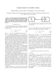
Figure 7: Ratio between wave amplitudes <strong>in</strong> moonpool and bas<strong>in</strong><br />
as a function of bas<strong>in</strong> wave period (least squares curve<br />
fit). Notice the resonance at T m 13 s.<br />
tion are 31 rad/s to 46 rad/s, [15].<br />
The frequency-dependent ratio between wave amplitudes <strong>in</strong>side<br />
the moonpool and <strong>in</strong> the bas<strong>in</strong> is illustrated <strong>in</strong> Figure 7.<br />
The data are experimental and based on a frequency-sweep<br />
us<strong>in</strong>g regular waves at 2 cm amplitude. We notice the characteristic<br />
resonance near the period T m 13s,orω m 483<br />
rad/s, see also [16].<br />
Typical vessel heave frequencies are <strong>in</strong> the range 40 <br />
ω heave 90 rad/s. The natural frequency of the heave motion<br />
of the vessel was found experimentally to be approximately<br />
ω heave<br />
48 rad/s, see also [16, 17].<br />
A first order model of the transfer function from the reference<br />
speed ż d<br />
to the motor speed ż m is<br />
ż m e 0010s<br />
´sµ <br />
ż d<br />
1 · 0020s<br />
(16)<br />
The time-delay is ma<strong>in</strong>ly due to digital communication between<br />
the motor drive and control units. At ω 63 rad/s the<br />
motor gives a phase loss of approximately 12 deg.<br />
feedback control bandwidth. The ma<strong>in</strong> performance measures<br />
of <strong>in</strong>terest are the wire tension and hydrodynamic<br />
forces on the payload. The m<strong>in</strong>imum value must never be<br />
less than zero to avoid high snatch loads, and the peak values<br />
and variance should be m<strong>in</strong>imized.<br />
4.1 Active heave compensation<br />
The objective of a heave compensator is to make the payload<br />
track a given trajectory <strong>in</strong> an Earth-fixed vertical reference<br />
system. This means that the payload motion will not be <strong>in</strong>fluenced<br />
by the heave motion of the vessel. This is implemented<br />
us<strong>in</strong>g feed-forward where an estimate ˙ẑ 0<br />
of the vessel’s vertical<br />
velocity (<strong>in</strong> an Earth-fixed vertical reference system) is<br />
added to the motor speed reference signal ż £ m commanded by<br />
the operator or a higher level control system:<br />
ż d<br />
ż £ m · ˙ẑ 0<br />
(17)<br />
The vessel vertical velocity ż 0<br />
can be estimated us<strong>in</strong>g an estimator<br />
which essentially <strong>in</strong>tegrates an accelerometer signal<br />
and removes bias us<strong>in</strong>g a high-pass filter because it can be assumed<br />
that the vessel oscillates vertically around zero Earthfixed<br />
position (mean sea level):<br />
˙ẑ 0´sµ <br />
H hp´sµ<br />
s<br />
¨z 0´sµ (18)<br />
where ¨z 0<br />
is the measured vessel acceleration and H hp´sµ is<br />
a 2nd order high-pass filter with cutoff frequency below the<br />
p. 7
significant wave frequencies:<br />
H hp´sµ<br />
<br />
s 2<br />
ω 2 c · 2 ¡ 045 ¡ ω cs · s 2 (19)<br />
with cutoff frequency ω c 137 rad/s, well below significant<br />
wave frequencies.<br />
4.2 <strong>Wave</strong> synchronization<br />
<strong>Wave</strong> amplitude measurements can be used <strong>in</strong> a feed-forward<br />
compensator to ensure that the payload motion is synchronized<br />
with the water motion <strong>dur<strong>in</strong>g</strong> the water entry phase.<br />
An objective is to m<strong>in</strong>imize variations <strong>in</strong> the hydrodynamic<br />
forces on the payload, f zd´z r µ, where<br />
f zd<br />
ρÇ ´z r µ z Z ´z<br />
z r µ z r r<br />
1<br />
2 ρC D A pz<br />
<br />
z r¬<br />
∂Z<br />
z r<br />
´z r µ<br />
∂z r<br />
<br />
z 2<br />
z r¬ d l ż r (20)<br />
This equation represents the dynamic part of (9). The first<br />
term of (20) is the Froude-Kriloff pressure force. The second<br />
term represents the contribution of the added mass, while the<br />
third term conta<strong>in</strong>s the slamm<strong>in</strong>g loads. The fourth term is<br />
the viscous drag on the payload. Rather than m<strong>in</strong>imiz<strong>in</strong>g this<br />
expression explicitly, we observe that a close to optimal solution<br />
is achieved by m<strong>in</strong>imiz<strong>in</strong>g variations <strong>in</strong> ż r , the relative<br />
vertical velocity of the payload and water. S<strong>in</strong>ce<br />
z r z ζ 0<br />
(21)<br />
frame). The factor κ´zµ accounts for the dependence of the<br />
water vertical velocity on water depth. S<strong>in</strong>ce the moonpool<br />
operates as a piston <strong>in</strong> a cyl<strong>in</strong>der, the water vertical velocity<br />
may be assumed to be approximately constant from the wave<br />
surface to the bottom of the moonpool, and decay exponentially<br />
below this po<strong>in</strong>t:<br />
κ´zµ<br />
<br />
<br />
1<br />
z h m<br />
(23)<br />
exp´ k´z h m µµ z h m<br />
S<strong>in</strong>ce this control should only be applied <strong>dur<strong>in</strong>g</strong> the water<br />
entry phase, we <strong>in</strong>troduce the factor α´zµ and blends the wave<br />
synchronization with heave compensation:<br />
ż d ż £ m · ˙ˆζ0 α´zµκ´zµ·˙ẑ 0 ´1 α´zµκ´zµµ (24)<br />
The position-dependent factor α´zµ goes smoothly from zero<br />
to one when the payload is be<strong>in</strong>g submerged, for example<br />
α´zµ<br />
<br />
<br />
<br />
0<br />
z 010<br />
10´z · 010µ 010 z 0<br />
1 z 0<br />
(25)<br />
The feedforward (24) conta<strong>in</strong>s both wave synchronization<br />
and heave compensation, and when z is large this expression<br />
co<strong>in</strong>cides with the heave compensator (17). Also notice that<br />
when the water <strong>in</strong>side the moonpool does not move (ζ 0,<br />
which gives ζ 0 z 0<br />
) the wave synchronization (24) also<br />
we get the approximation ż r ż<br />
˙ζ0 κ´zµ by assum<strong>in</strong>g that<br />
co<strong>in</strong>cides with the heave compensator (17) for all z.<br />
the wave amplitude decays with depth accord<strong>in</strong>g to the function<br />
κ´zµ. Hence, wave synchronization is achieved by the<br />
feed-forward compensator<br />
ż d<br />
ż £ m · ˙ˆζ0 κ´zµ (22)<br />
where ˙ˆζ0 is an estimate of the velocity of the wave surface<br />
elevation <strong>in</strong>side the moonpool (<strong>in</strong> a vessel-fixed coord<strong>in</strong>ate<br />
The wave amplitude ζ 0<br />
relative to a vessel-fixed position <strong>in</strong>side<br />
the moonpool is measured. The wave amplitude velocity<br />
˙ζ 0<br />
is estimated by filter<strong>in</strong>g and (numerical) differentiation:<br />
˙ˆζ 0´sµ sH lp´sµH notch´sµζ 0´sµ (26)<br />
The low pass filter H lp´sµ is composed of a 2nd order critically<br />
damped filter at 60 rad/s and a 2nd order critically<br />
p. 8
damped filter at 200 rad/s. In order to avoid excit<strong>in</strong>g the wire<br />
resonance, we have <strong>in</strong>troduced a notch filter<br />
H notch´sµ s2 · 2 ¡ 01 ¡ ω n · ω 2 n<br />
s 2 · 2 ¡ 05 ¡ ω n · ω 2 n<br />
(27)<br />
typically tuned at ω n ω 3<br />
.<br />
In the experiments we used<br />
ω n 37 rad/s. A block diagram illustrat<strong>in</strong>g the wave synchronization<br />
is given <strong>in</strong> Figure 8.<br />
Figure 9: MCLab bas<strong>in</strong>: 40 m ¢ 6.45 m ¢ 1.5 m.<br />
see Figure 7, and the wave amplitude <strong>in</strong>side the moonpool<br />
is about 2 times the bas<strong>in</strong> wave amplitude. The<br />
equivalent wave height <strong>in</strong> full scale is around H s 11<br />
m.<br />
¯ Spherical payload <strong>in</strong> regular waves with period T <br />
10 s and amplitude A 68 cm. At this frequency<br />
Figure 8: <strong>Wave</strong> synchronization block diagram.<br />
there is no resonance. The equivalent wave height <strong>in</strong><br />
full scale is around H s 41m.<br />
5 Experimental results<br />
In this section we summarize experimental results with the<br />
heave compensation and wave synchronization control strategies<br />
described above. More data and results with several payloads<br />
<strong>in</strong> regular and irregular waves can be found <strong>in</strong> [14]. The<br />
experiments were carried out <strong>in</strong> the MCLab [6] at <strong>NTNU</strong>, see<br />
Figure 9.<br />
The two scenarios we present here represent typical performance<br />
improvements that can be achieved:<br />
¯ Spherical payload <strong>in</strong> regular waves with period T <br />
We present both raw and filtered wire tension data. The filtered<br />
data conta<strong>in</strong>s ma<strong>in</strong>ly components <strong>in</strong> the frequency band<br />
between 3.1 rad/s and 9.4 rad/s, where the significant wave<br />
motion is located (the filter<strong>in</strong>g is carried out us<strong>in</strong>g 4th order<br />
filters with no phase shift). This filter<strong>in</strong>g allows the effects<br />
of the wave synchronization to be separated from other effects,<br />
s<strong>in</strong>ce this is the frequency band where the wave synchronization<br />
is effective. It is therefore natural to verify the<br />
performance of the wave synchronization on the filtered data,<br />
neglect<strong>in</strong>g low-frequency components due to buoyancy and<br />
high-frequency components due to measurement noise and<br />
125 s and amplitude A 18 cm.<br />
This wave fre-<br />
wire/suspension resonances.<br />
Still, it is also of <strong>in</strong>terest to<br />
quency is close to the moonpool resonance frequency,<br />
evaluate the performance of the wave synchronization with<br />
p. 9
espect to excitation of the wire/suspension resonance. This<br />
evaluation is, however, not straightforward to carry out s<strong>in</strong>ce<br />
the laboratory model does not conta<strong>in</strong> passive heave compensation<br />
or damp<strong>in</strong>g. Moreover, the excitations caused by<br />
signal noise and w<strong>in</strong>ch motor drive are not directly scalable<br />
to a full scale implementation and must be considered <strong>in</strong> the<br />
context of the technology used for implementation. Thus, we<br />
will base our conclusions ma<strong>in</strong>ly on the filtered data.<br />
5.1 Regular waves at T 125 s and A 18 cm<br />
Figure 10 shows the payload position and wire tension for<br />
test series B (two tests A and B are carried out at each sea<br />
state to verify repeatability) with the spherical payload, with<br />
and without control. The follow<strong>in</strong>g observations and remarks<br />
can be made:<br />
¯ The wave synchronization reduces the tension standard<br />
deviation by 25.2 % <strong>in</strong> test A and 21.4 % <strong>in</strong> test<br />
B, compared to no control, when consider<strong>in</strong>g filtered<br />
data. <strong>Wave</strong> synchronization <strong>in</strong> comb<strong>in</strong>ation with heave<br />
compensation reduces the tension standard deviation<br />
by 22.0 % <strong>in</strong> test A and 21.8 % <strong>in</strong> test B, compared to<br />
no control, when consider<strong>in</strong>g filtered data.<br />
¯ The peak m<strong>in</strong>imum tension is changed from 1.21 N to<br />
1.58 N us<strong>in</strong>g wave synchronization <strong>in</strong> test A and from<br />
1.36 N to 1.58 N <strong>in</strong> test B, compared to no control,<br />
when consider<strong>in</strong>g filtered data. This is beneficial as it<br />
reduces the possibility of wire snatch. The peak maximum<br />
tension is somewhat <strong>in</strong>creased with the wave synchronization.<br />
¯ The use of heave compensation does not give any significant<br />
reduction of tension variability <strong>in</strong> this sea state.<br />
However, it gives significant reduction of the standard<br />
deviation of the payload acceleration. The reason for<br />
this is that the heave motion is fairly small compared<br />
to the resonant moonpool water motion.<br />
¯ When consider<strong>in</strong>g the unfiltered data, similar qualitative<br />
conclusions can be made.<br />
¯ For the pump-<strong>in</strong>-frame payload, the wave synchronization<br />
reduces the tension standard deviation by 7.2 % <strong>in</strong><br />
test A and 12.8 % <strong>in</strong> test B, compared to no control,<br />
when consider<strong>in</strong>g filtered data. <strong>Wave</strong> synchronization<br />
<strong>in</strong> comb<strong>in</strong>ation with heave compensation reduces the<br />
tension standard deviation by 8.9 % <strong>in</strong> test A and 15.3<br />
% <strong>in</strong> test B, compared to no control, when consider<strong>in</strong>g<br />
filtered data.<br />
5.2 Regular waves at T 10 s and A 68 cm<br />
Figure 11 shows the payload position and wire tension for<br />
test series B with the spherical payload, with and without<br />
control. We make the follow<strong>in</strong>g observations and remarks:<br />
¯ The wave synchronization reduces the tension standard<br />
deviation by 31.0 % <strong>in</strong> test A and 33.1 % <strong>in</strong> test<br />
B, compared to no control, when consider<strong>in</strong>g filtered<br />
data. <strong>Wave</strong> synchronization <strong>in</strong> comb<strong>in</strong>ation with heave<br />
compensation reduces the tension standard deviation<br />
by 48.1 % <strong>in</strong> test A and 54.2 % <strong>in</strong> test B, compared to<br />
no control, when consider<strong>in</strong>g filtered data.<br />
¯ The m<strong>in</strong>imum tension is changed from 1.36 N to 1.23<br />
N us<strong>in</strong>g wave synchronization <strong>in</strong> test A and from 1.59<br />
p. 10
N to 1.67 N <strong>in</strong> test B, compared to no control, when<br />
consider<strong>in</strong>g filtered data.<br />
¯ The use of heave compensation alone gives significant<br />
reduction of tension variability <strong>in</strong> this very rough sea<br />
state, namely 50.3 % <strong>in</strong> test A and 25.9 % <strong>in</strong> test B.<br />
This <strong>in</strong>dicates that significant reduction <strong>in</strong> tension variance<br />
can be achieved by either heave compensation or<br />
wave synchronization, but largest reduction is achieved<br />
by comb<strong>in</strong><strong>in</strong>g them.<br />
¯ When consider<strong>in</strong>g the unfiltered data, similar qualitative<br />
conclusions can be made <strong>in</strong> most cases.<br />
¯ For the pump-<strong>in</strong>-frame payload the wave synchronization<br />
reduces the tension standard deviation by 36.9 %<br />
<strong>in</strong> test A and 34.5 % <strong>in</strong> test B. <strong>Wave</strong> synchronization <strong>in</strong><br />
comb<strong>in</strong>ation with heave compensation reduces the tension<br />
standard deviation by 61.4 % <strong>in</strong> test A and 53.2 %<br />
<strong>in</strong> test B, when consider<strong>in</strong>g filtered data.<br />
5.3 Discussion<br />
<strong>Wave</strong> synchronization, either alone or <strong>in</strong> comb<strong>in</strong>ation with<br />
heave compensation, significantly reduces wire tension variability<br />
and peak values <strong>in</strong> a large majority of the tests. However,<br />
under some sea states and for some payloads, no or only<br />
small improvement was experienced. The experiments with<br />
regular waves showed good repeatability, giv<strong>in</strong>g consistent<br />
conclusions with different experiments under the same sea<br />
state.<br />
Overall, the results are encourag<strong>in</strong>g, show<strong>in</strong>g that wave synchronization<br />
has a significant benefit <strong>in</strong> terms of reduced tension<br />
variability and peaks at least under some sea states and<br />
with some payloads. Some limitations to performance and<br />
sources to uncerta<strong>in</strong>ty has been identified:<br />
First, the feedforward approach leads to a phase error, due to<br />
the dynamics of the motor and signal filter<strong>in</strong>g. In our experimental<br />
setup this error is significant, and not compensated<br />
for. For a wave period of 1.0 s, the phase loss <strong>in</strong> the motor<br />
is 12 degrees and the phase loss <strong>in</strong> the filter<strong>in</strong>g of the wave<br />
amplitude measurement is about 25 deg. The total phase loss<br />
is around 37 deg. It is therefore clear that the use of some<br />
model-based predictor of the wave amplitude may lead to<br />
significant improvement of performance.<br />
Second, the wire/suspension resonance is be<strong>in</strong>g excited, also<br />
without the use of wave synchronization or heave compensation.<br />
The use of heave compensation or heave compensation<br />
reduces the excitations of the resonance <strong>in</strong> most cases with<br />
the spherical payload, while the excitations of the resonance<br />
seems to be typically <strong>in</strong>creased with the pump-<strong>in</strong>-frame payload.<br />
There are several possible sources for these excitations:<br />
1. Even with constant speed reference the AC motor drive<br />
exhibit oscillations with significant frequency components<br />
<strong>in</strong> area where the resonance frequency is.<br />
2. The water flow <strong>in</strong>side the moonpool or the heave motion<br />
of the vessel may conta<strong>in</strong> frequency components<br />
that give hydrodynamic forces that excite the wire resonance.<br />
3. Measurement noise may excite the resonance frequency.<br />
S<strong>in</strong>ce there is very little damp<strong>in</strong>g <strong>in</strong> the suspension<br />
and the resonance frequency is less than a<br />
decade above from typical wave frequencies, any filterp.<br />
11
8<br />
<strong>Wave</strong> synchronization<br />
8<br />
Heave compensation<br />
6<br />
6<br />
tension (N)<br />
4<br />
tension (N)<br />
4<br />
2<br />
2<br />
0<br />
260 265 270 275 280<br />
time (s)<br />
0<br />
185 190 195 200<br />
time (s)<br />
<strong>Wave</strong> sychronization and heave compensation<br />
8<br />
8<br />
No control<br />
6<br />
6<br />
tension (N)<br />
4<br />
tension (N)<br />
4<br />
2<br />
2<br />
0<br />
95 100 105 110 115<br />
time (s)<br />
<strong>Wave</strong> synchronization<br />
0.8<br />
0<br />
0.8<br />
345 350 355 360 365<br />
time (s)<br />
Heave compensation<br />
0.6<br />
0.6<br />
motor position (m)<br />
0.4<br />
0.2<br />
0<br />
motor position (m)<br />
0.4<br />
0.2<br />
0<br />
−0.2<br />
−0.2<br />
260 265 270 275 280<br />
time (s)<br />
<strong>Wave</strong> sychronization and heave compensation<br />
0.8<br />
0.8<br />
185 190 195 200<br />
time (s)<br />
No control<br />
0.6<br />
0.6<br />
motor position (m)<br />
0.4<br />
0.2<br />
0<br />
motor position (m)<br />
0.4<br />
0.2<br />
0<br />
−0.2<br />
−0.2<br />
95 100 105 110 115<br />
time (s)<br />
345 350 355 360 365<br />
time (s)<br />
Figure 10: Experimental results with regular waves at T 125 s and A 18 cm, spherical payload, test B. For the wire tension we show<br />
both raw data (th<strong>in</strong> l<strong>in</strong>es) and low-pass filtered data (thick l<strong>in</strong>es). The payload position (measured us<strong>in</strong>g the motor shaft encoder)<br />
is <strong>in</strong> a vessel-fixed coord<strong>in</strong>ate frame, with zero at mean sea level.<br />
p. 12
8<br />
<strong>Wave</strong> synchronization<br />
8<br />
Heave compensation<br />
6<br />
6<br />
tension (N)<br />
4<br />
tension (N)<br />
4<br />
2<br />
2<br />
0<br />
260 265 270 275 280<br />
time (s)<br />
0<br />
185 190 195 200 205<br />
time (s)<br />
<strong>Wave</strong> sychronization and heave compensation<br />
8<br />
8<br />
No control<br />
6<br />
6<br />
tension (N)<br />
4<br />
tension (N)<br />
4<br />
2<br />
2<br />
0<br />
110 115 120 125 130<br />
time (s)<br />
0<br />
335 340 345 350<br />
time (s)<br />
0.8<br />
<strong>Wave</strong> synchronization<br />
0.8<br />
Heave compensation<br />
0.6<br />
0.6<br />
motor position (m)<br />
0.4<br />
0.2<br />
0<br />
motor position (m)<br />
0.4<br />
0.2<br />
0<br />
−0.2<br />
−0.2<br />
260 265 270 275 280<br />
time (s)<br />
185 190 195 200 205<br />
time (s)<br />
<strong>Wave</strong> sychronization and heave compensation<br />
0.8<br />
0.8<br />
No control<br />
0.6<br />
0.6<br />
motor position (m)<br />
0.4<br />
0.2<br />
0<br />
motor position (m)<br />
0.4<br />
0.2<br />
0<br />
−0.2<br />
−0.2<br />
110 115 120 125 130<br />
time (s)<br />
335 340 345 350<br />
time (s)<br />
Figure 11: Experimental results with regular waves at T 100 s and A 68 cm, spherical payload, test B. For the wire tension we show<br />
both raw data (th<strong>in</strong> l<strong>in</strong>es) and low-pass filtered data (thick l<strong>in</strong>es). The payload position (measured us<strong>in</strong>g the motor shaft encoder)<br />
is <strong>in</strong> a vessel-fixed coord<strong>in</strong>ate frame, with zero at mean sea level.<br />
p. 13
<strong>in</strong>g will lead to phase loss as described above. A further<br />
complication is that the resonance frequency depend<br />
on payload mass and position-dependent hydrodynamic<br />
properties such as added mass. Improvements<br />
may be expected by adaptive notch filter<strong>in</strong>g, <strong>in</strong> comb<strong>in</strong>ation<br />
with wave prediction. Obviously, the technical<br />
solutions for wave measurements, signal transmission<br />
and electronics may be modified to reduce the overall<br />
noise level. Noise is amplified due to numerical differentiation<br />
when comput<strong>in</strong>g the wave surface speed<br />
from the wave amplitude measurements, and alternative<br />
methods to measur<strong>in</strong>g the relative velocity of the<br />
water and payload are of <strong>in</strong>terest.<br />
may have an effect for streaml<strong>in</strong>ed bodies, like the sphere, but<br />
may most likely be neglected for bluff bodies s<strong>in</strong>ce the separation<br />
po<strong>in</strong>t (of vortices) becomes the same for scaled and<br />
full scale bluff bodies. Damp<strong>in</strong>g is normally over predicted <strong>in</strong><br />
model scale experiments due to viscous effects. This causes<br />
an under prediction of the response which is important to take<br />
<strong>in</strong>to account when transferr<strong>in</strong>g the experimental data to full<br />
scale. The effects from elasticity are well taken care of t<strong>in</strong><br />
the model scale s<strong>in</strong>ce all frequencies are scaled correctly.<br />
6 Conclusions<br />
It is shown via scale model experiments that the performance<br />
of offshore moonpool crane operations can be significantly<br />
improved by wave synchronization <strong>in</strong> comb<strong>in</strong>ation<br />
with heave compensation.<br />
This can be implemented as a<br />
The experiments are scaled with respect to the Froude number,<br />
a dimensionless number def<strong>in</strong>ed as the fraction between<br />
the <strong>in</strong>ertial and gravitational forces Fr z Ô gr where r is<br />
a characteristic radius. Thus, all elastic effects are well accounted<br />
for as long as the frequencies are properly scaled.<br />
Frequency <strong>in</strong> the model scale f m is scaled with λ 1 2 , that is<br />
feedforward compensator with<strong>in</strong> an active heave compensation<br />
system, us<strong>in</strong>g measurement of the wave amplitude <strong>in</strong> the<br />
moonpool.<br />
Acknowledgements<br />
f λ<br />
1<br />
2 f m where λ 30 is the scale used <strong>in</strong> the experiments.<br />
Viscous effects are normally scaled with respect to<br />
the Reynolds number . The Reynolds number is dimensionless<br />
variable which represents the fraction between <strong>in</strong>ertia<br />
and viscous effects def<strong>in</strong>ed as follows: Re ζ rν where ν is<br />
k<strong>in</strong>ematic viscosity. The relationship between full scale and<br />
the model scale Reynolds numbers when us<strong>in</strong>g Froude scale<br />
becomes Re λ 3 2 Re m where the subscript m denotes model<br />
scale. A typical Reynolds number <strong>in</strong> the experiments is 5¡10 4<br />
while the Reynolds number <strong>in</strong> the full scale case normally is<br />
<strong>in</strong> the range of 10 6 . This discrepancy <strong>in</strong> Reynolds number<br />
<br />
The authors are grateful to Mar<strong>in</strong>tek for k<strong>in</strong>d assistance <strong>dur<strong>in</strong>g</strong><br />
the experiments.<br />
References<br />
[1] NSLT, The 5th North Sea Offshore <strong>Crane</strong> Conference,<br />
Aberdeen, Scotland, Norwegian Society of Lift<strong>in</strong>g Technology<br />
(NSLT), 2000.<br />
[2] NSLT, Underwater Lift<strong>in</strong>g Operations, Stavanger,<br />
Norway (<strong>in</strong> Norwegian), Norwegian Society of Lift<strong>in</strong>g Technology<br />
(NSLT), 2000.<br />
[3] NSLT, The 3th International Offshore <strong>Crane</strong> Conferp.<br />
14
ence, Kristiansand, Norway, Norwegian Society of Lift<strong>in</strong>g<br />
Tech. Rep. 2001-12-T, http://www.itk.ntnu.no/research/-<br />
Technology (NSLT), 1998.<br />
HydroLab/reports/hydrolaunch model.pdf,<br />
Department of<br />
[4] S. I. Sagatun, T. I. Fossen, and K. P. L<strong>in</strong>degaard, “Inertance<br />
control of underwater <strong>in</strong>stallations,” <strong>in</strong> Prepr<strong>in</strong>t IFAC<br />
CAMS, Glasgow, Scotland, 2001.<br />
[5] U. A. Korde, “Active heave compensation on drillships<br />
<strong>in</strong> irregular waves,” Ocean Eng<strong>in</strong>eer<strong>in</strong>g, vol. 25, pp.<br />
541–561, 1998.<br />
[6] “MCLab - Mar<strong>in</strong>e Cybernetcs Laboratory, Trondheim,”<br />
http://www.itk.ntnu.no/mar<strong>in</strong>kyb/MCLab/, 2002.<br />
[7] S. I. Sagatun, T. A. Johansen, T. I. Fossen, and F. G.<br />
Nielsen, “<strong>Wave</strong> synchronizat<strong>in</strong>g crane control <strong>dur<strong>in</strong>g</strong> water<br />
entry <strong>in</strong> offshore moonpool operations,” <strong>in</strong> Proc. IEEE Conf.<br />
<strong>Control</strong> Applications, Glasgow, 2002.<br />
[8] O. M. Falt<strong>in</strong>sen, Sea Loads on Ships and Offshore<br />
Structures, Cambridge University Press, New York, 1990.<br />
[9] J. N. Newman, Mar<strong>in</strong>e Hydrodynamics, Cambridge,<br />
MA: MIT Press, 1977.<br />
Eng<strong>in</strong>eer<strong>in</strong>g Cybernetics, <strong>NTNU</strong>, Trondheim, Norway, 2001.<br />
[14] T. A. Johansen and T. I. Fossen, “Observer and<br />
controller design for an offshore crane moonpool system,”<br />
Tech. Rep. 2001-13-T, http://www.itk.ntnu.no/research/-<br />
HydroLab/reports/hydrolaunch control.pdf, Department of<br />
Eng<strong>in</strong>eer<strong>in</strong>g Cybernetics, <strong>NTNU</strong>, Trondheim, Norway, 2001.<br />
[15] T. A. Johansen and T. I. Fossen, “HydroLaunch free<br />
decay tests,” Tech. Rep. 2001-18-T, http://www.itk.ntnu.no/-<br />
research/HydroLab/reports/hydrolaunch free decay.pdf, Department<br />
of Eng<strong>in</strong>eer<strong>in</strong>g Cybernetics, <strong>NTNU</strong>, Trondheim,<br />
Norway, 2001.<br />
[16] F. G. Nielsen, “Coupled hydrodynamics for<br />
the HydroLaunch vessel with load,” Work<strong>in</strong>g note,<br />
Norsk Hydro, Exploration and Production, Bergen, Norway,<br />
http://www.itk.ntnu.no/research/HydroLab/reports/-<br />
HydroLab dynamics.pdf, 2002.<br />
[17] M. P. Fard and F. G. Nielsen, “Simulation<br />
of coupled vessel-load dynamics,”<br />
Tech. Rep.<br />
[10] DnV, Rules for Plann<strong>in</strong>g and Execution of Mar<strong>in</strong>e Operations,<br />
DnV, Norway, 2000.<br />
[11] M. Greenhow and L. Yanbao, “Added masses for circular<br />
cyl<strong>in</strong>ders near or penetrat<strong>in</strong>g fluid boundaries - review,<br />
NH-00036960, http://www.itk.ntnu.no/research/HydroLab/-<br />
reports/Fard2002.pdf, Norsk Hydro, Exploration and Production,<br />
Bergen, Norway, 2001.<br />
extension and application to water-entry, -exit and slamm<strong>in</strong>g,”<br />
J. Ocean Eng<strong>in</strong>eer<strong>in</strong>g, vol. 14, pp. 325–348, 1987.<br />
[12] W. Price and R. Bishop, Probabilistic Theory of Ship<br />
Dynamics, London, UK: Chapman and Hall, 1974.<br />
[13] T. I. Fossen and T. A. Johansen, “Modell<strong>in</strong>g<br />
and identification of offshore crane-rig system,”<br />
p. 15