Cascaded lemma for set-stable systems
Cascaded lemma for set-stable systems
Cascaded lemma for set-stable systems

You also want an ePaper? Increase the reach of your titles
YUMPU automatically turns print PDFs into web optimized ePapers that Google loves.
Cascade <strong>lemma</strong> <strong>for</strong> <strong>set</strong>-<strong>stable</strong> <strong>systems</strong><br />
Johannes Tjønnås ∗ , Antoine Chaillet ∗∗ , Elena Panteley ∗∗ and Tor Arne Johansen ∗<br />
∗ Department of Engineering Cybernetics, Norwegian University of Science and Technology, Trondheim, Norway.<br />
∗∗ LSS - Supélec, Gif sur Yvette, France.<br />
Abstract— A previous result about uni<strong>for</strong>m global asymptotic<br />
stability (UGAS) of the equilibrium of a cascaded time-varying<br />
<strong>systems</strong>, is here also shown to hold <strong>for</strong> closed (not necessarily<br />
compact) <strong>set</strong>s composed by <strong>set</strong>-<strong>stable</strong> sub<strong>systems</strong> of a cascade.<br />
In view of this result an optimal control allocation approach is<br />
discussed.<br />
I. INTRODUCTION<br />
The work presented in this note is based on a result from<br />
[1] where uni<strong>for</strong>m global asymptotic stability (UGAS) of<br />
cascaded system<br />
ẋ 1 = f 1 (t, x 1 ) + g(t, x) (1a)<br />
ẋ 2 = f 2 (t, x 2 ) (1b)<br />
where x := (x T 1, x T 2) T , is concluded <strong>for</strong> the case g(t, x) =<br />
g 1 (t, x)x 2 , if the both origins of ẋ 1 = f 1 (t, x 1 ) and ẋ 2 =<br />
f 2 (t, x 2 ) are UGAS and the solutions of the cascaded system<br />
are uni<strong>for</strong>mly globally bounded (UGB). This result motivates<br />
a modular approach where the sub<strong>systems</strong> can be analyzed<br />
separately and conclusions about the properties of the cascaded<br />
system may be drawn based on the interconnection<br />
term g(t, x) instead of analyzing the cascade as one system,<br />
which in many cases induces complexity. Background on<br />
stability analysis of cascaded <strong>systems</strong> can be found in [2],<br />
[3], [4], [5], [6], [7], [8] and references therein.<br />
Roughly speaking, we show that if a <strong>set</strong> is uni<strong>for</strong>m global<br />
asymptotic <strong>stable</strong> (UGAS) with respect to a system, then the<br />
composed <strong>set</strong> generated by a cascade of two such <strong>systems</strong><br />
is itself UGAS under the assumption that the solutions of<br />
the cascaded system are UGB with respect to the composed<br />
<strong>set</strong>. We also include a more practical result where UGB is<br />
concluded under a certain growth condition.<br />
Our motivation <strong>for</strong> studying stability properties <strong>for</strong> <strong>set</strong>s<br />
rests mainly on studying applications that involve solving an<br />
optimal control allocation problem. We consider a dynamic<br />
control allocation approach that is of special interest <strong>for</strong><br />
<strong>systems</strong> that exhibit fast dynamics. This control allocation<br />
approach, where stability of optimal <strong>set</strong>s is addressed, was<br />
first considered in [9] and later in [10] by including uncertain<br />
parameters, to be adapted, in the effector model. By establishing<br />
the result presented here the assumptions in [9] and<br />
[10] can be relaxed and a wider class of nonlinear <strong>systems</strong><br />
may be considered. An idea of how this can be done is shown<br />
in section IV.<br />
When the functions f 1 , f 2 and g from (1) are locally<br />
Lipschitz, this class of nonlinear time-varying <strong>systems</strong> can<br />
<br />
z 2<br />
<br />
|z | 2 O 2<br />
<br />
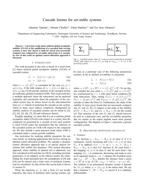
Fig. 1. <strong>Cascaded</strong> system, where Σ 1 is the perturbed system that is assumed<br />
UGAS with respect to a <strong>set</strong>, O 1 , as long as |z 2 | O2<br />
= 0. Σ 2 is the<br />
perturbing system.<br />
be seen as a particular case of the following autonomous<br />
<strong>systems</strong>, as far as uni<strong>for</strong>m <strong>set</strong>-stability is concerned:<br />
ż 1 = F 1 (z 1 ) + G(z) (2a)<br />
ż 2 = F 2 (z 2 ) (2b)<br />
where z 1 ∈ R q 1<br />
, z 2 ∈ R q 2<br />
, z := (z1, T z2) T T ∈ R q . To see this,<br />
just consider the case when z 1 = (t, x T 1) T and z 2 = (t, x T 2) T<br />
are synchronized by, ṫ = 1 with same initial conditions <strong>for</strong><br />
both sub<strong>systems</strong>. Then, letting F 1 (z 1 ) = (1, f 1 (t, x 1 ) T ) T ,<br />
G(z) = (0, g(t, x) T ) T and F 2 (z 2 ) = (1, f 2 (t, x 2 ) T ) T , the<br />
cascade (1) takes the <strong>for</strong>m (2). Furthermore, the study of the<br />
stability of some given closed (but not necessarily compact)<br />
<strong>set</strong>s N 1 and N 2 <strong>for</strong> (1) reduces to the study of the stability<br />
of O 1 := R ≥0 × N 1 and O 2 := R ≥0 × N 2 <strong>for</strong> the system<br />
(2). This structure of the <strong>set</strong>s O 1 and O 2 should however<br />
be seen as a particular case, and the <strong>set</strong>-stability properties<br />
that we expose in the sequel englobe much more general<br />
configurations. The diagram in Figure 1, represents a general<br />
cascaded system.<br />
A. Notation<br />
II. PRELIMINARY DEFINITIONS AND RESULTS<br />
The function α : R ≥0 → R ≥0 is of class K if it is<br />
continuous, strictly increasing and α(0) = 0. α is of class<br />
K ∞ if in addition α(s) → ∞ as s → ∞. β : R ≥0 ×<br />
R ≥0 → R ≥0 is a class KL function if, <strong>for</strong> each fixed t,<br />
the mapping β(·, t) is of class K and <strong>for</strong> each fixed s the<br />
mapping β(s, ·) is continuous, decreasing and tends to zero<br />
as its argument tends to +∞. |·| denotes the Euclidian norm<br />
and |·| A ′ : R q → R ≥0 denotes the distance from a point<br />
z ∈ R q to a <strong>set</strong> A ′ ⊂R q , |z| A ′ := inf {|z − y| : y ∈ A ′ } .<br />
The solution of an autonomous dynamic system is denoted<br />
by z(t, z 0 ) where z 0 = z(t 0 , z 0 ) is the initial state. We say<br />
that a function V : R q → R ≥0 is smooth if it is infinitely<br />
differentiable.
B. Definitions<br />
The definitions that follows are either motivated by or can<br />
be found in [11] and [12]. They pertain to <strong>systems</strong> of the<br />
<strong>for</strong>m<br />
ż = F (z) , (3)<br />
where F : D → R q is locally Lipschitz with D ⊂ R q .<br />
Definition 1: The system (3) is said to be <strong>for</strong>ward complete<br />
if, <strong>for</strong> each z 0 ∈ D, the solution z(·, z 0 ) ∈ D is defined<br />
on R ≥0 .<br />
Definition 2: The system (3) is said to be finite escape<br />
time detectable through |·| A<br />
, if any solution, z(t, z 0 ) ∈ D,<br />
which is right maximally defined on a bounded interval<br />
[0, T ), satisfies lim t↗T |z(t, z 0 )| A<br />
= ∞.<br />
Definition 3: For the system (3), the closed <strong>set</strong> A ⊂ D is<br />
Uni<strong>for</strong>mly Stable (US) if the system (3) is <strong>for</strong>ward complete,<br />
and there exists a function ν ∈ K and a constant c > 0 such<br />
that, ∀ |z 0 | A<br />
< c,<br />
|z(t, z 0 )| A<br />
≤ ν(|z 0 | A<br />
), ∀t ≥ 0 . (4)<br />
Definition 4: For the system (3), when D = R q , then the<br />
closed <strong>set</strong> A ⊂ R q is Uni<strong>for</strong>mly Globally Stable (UGS) if<br />
the system (3) is <strong>for</strong>ward complete and (4) is satisfied with<br />
ν ∈ K ∞ and <strong>for</strong> any z 0 ∈ R q .<br />
Definition 5: For the system (3), the closed <strong>set</strong> A ⊂ D<br />
is Uni<strong>for</strong>mly Attractive (UA) if the system (3) is <strong>for</strong>ward<br />
complete, there exists constant c > 0, such that <strong>for</strong> all<br />
|z 0 | A<br />
< c and any µ > 0 there exists T = T (µ) > 0,<br />
such that<br />
|z 0 | A<br />
≤ c, t ≥ T ⇒ |z(t, z 0 )| A<br />
≤ µ (5)<br />
Definition 6: For the system (3), when D = R q , then the<br />
closed <strong>set</strong> A ⊂ R q is Uni<strong>for</strong>mly Globally Attractive (UGA)<br />
if the system (3) is <strong>for</strong>ward complete, and <strong>for</strong> each pair of<br />
strictly positive numbers (c, µ) there exists T = T (c, µ) > 0<br />
such that <strong>for</strong> all z 0 ∈ R q , (5) holds.<br />
Definition 7: For the system (3), the closed <strong>set</strong> A is<br />
Uni<strong>for</strong>mly Asymptotically Stable (UAS) if it is US and UA.<br />
Definition 8: For the system (3), when D = R q , the closed<br />
<strong>set</strong> A is Uni<strong>for</strong>mly Globally Asymptotically Stable (UGAS)<br />
if it is UGS and UGA.<br />
Provided that (3) is <strong>for</strong>ward complete, this definition is<br />
well known to be equivalent to the following KL characterization<br />
(see e.g. [12], [13]): There exists a class KL function<br />
β such that, <strong>for</strong> all z 0 ∈ R q , |z(t, z 0 )| A ≤ β(|z 0 | A , t − 0)<br />
<strong>for</strong> all t ≥ 0.<br />
From [14], we adapt the definition of uni<strong>for</strong>m boundedness<br />
of solutions to the case when A is not reduced to {0}.<br />
Definition 9: The solutions of system (3) are said to be<br />
Uni<strong>for</strong>mly Bounded (UB) with respect to a closed <strong>set</strong> A ⊂<br />
D if, there exist a positive constant c, such that <strong>for</strong> every<br />
positive constant r < c there is a positive constant ¯c = ¯c(r),<br />
such that<br />
|z 0 | A<br />
≤ r ⇒ |z(t, z 0 )| A<br />
≤ ¯c , ∀t ≥ 0 . (6)<br />
Definition 10: The solutions of system (3), where<br />
D = R q , are said to be Uni<strong>for</strong>mly Globally Bounded (UGB)<br />
with respect to a closed <strong>set</strong> A ⊂ R q if, <strong>for</strong> every r ∈ R ≥0 ,<br />
there is a positive constant ¯c = ¯c(r) such that (6) is satisfied.<br />
It can easily be shown that this is equivalent to the<br />
existence of a nonnegative constant µ and of a class K ∞<br />
function η such that, <strong>for</strong> all z 0 ∈ R q ,<br />
|z(t, z 0 )| A ≤ η(|z 0 | A ) + µ , ∀t ≥ 0 .<br />
In what follows, O 1 ⊂ R q 1<br />
and O 2 ⊂ R q 2<br />
are closed (not<br />
necessarily bounded) <strong>set</strong>s and A = O 1 × O 2 .<br />
The <strong>set</strong>-stability analysis of (2) is done under the following<br />
assumptions.<br />
Assumption 1. The functions F 1 , F 2 and G are locally<br />
Lipschitz.<br />
Assumption 2. The cascade (2) is <strong>for</strong>ward complete.<br />
Assumption 3. There exist a continuous function G 1 :<br />
R ≥0 → R ≥0 and a class K function G 2 such that, <strong>for</strong> all<br />
z ∈ R q ,<br />
|G(z)| ≤ G 1 (|z| A<br />
)G 2 (|z 2 | O2 ).<br />
Assumption 4. There exists a continuously differentiable<br />
Lyapunov function ¯V 1 : R q 1<br />
→ R ≥0 , class K ∞ functions ᾱ 1 ,<br />
ᾱ 2 and ᾱ 3 , and a continuous function ¯ς : R ≥0 → R ≥0 such<br />
that, <strong>for</strong> all z 1 ∈ R q1 ,<br />
ᾱ 1 (|z 1 | O1 ) ≤ ¯V 1 (z 1 ) ≤ ᾱ 2 (|z 1 | O1 ) (7)<br />
∂ ¯V 1<br />
∂z 1<br />
(z 1 )F 1 (z 1 ) ≤ −ᾱ 3 (|z 1 | O1 ) (8)<br />
∂ ¯V 1<br />
∣ (z 1 )<br />
∂z 1<br />
∣ ≤ ¯ς ( )<br />
|z 1 | O1 . (9)<br />
It is worth underlining that the existence of a smooth<br />
Lyapunov function satisfying (7) and (8) follows directly<br />
from [12] or [13] if and only if O 1 is UGAS <strong>for</strong> ż 1 = F 1 (z 1 ).<br />
However, the bound (9) on the gradient may not be trivial,<br />
which justifies this assumption.<br />
Remark 1: For the special case where z 1 = (t, x T 1) T , the<br />
bound (9) will be reduced to<br />
∂ ¯V 1<br />
∣ (z 1 )<br />
∂x 1<br />
∣ ≤ ¯ς ( )<br />
|z 1 | O1 . (10)<br />
This is due to G(z) = (0, g(t, x) T ) T ∣, and the term of interest<br />
in our analysis is: ∂ ¯V 1<br />
∂z 1<br />
G(z) ≤ ∣ ∂ ¯V 1 ∣∣<br />
∂x 1<br />
|g(t, x)| .
√<br />
III. MAIN RESULT<br />
where ν(·) := α1 −1 2(·) + ˜β(·, 0)) 2 + β 2 (·, 0) 2 is a class<br />
Lemma 1. Let O 1 and O 2 be some closed sub<strong>set</strong>s of K ∞ function. UGS of A follows.<br />
R q1 and R q2 respectively. Assume that O 2 is UGAS with To prove uni<strong>for</strong>m global attractiveness, consider any positive<br />
constants ε 1 and r such that ε 1 < r and let T 1 (ε 1 , r) ≥ 0<br />
respect to the system (2b) and that the solutions of system<br />
(2) are UGB with respect to A := O 1 × O 2 . Then, under be such that 2 ˜β(r, T 1 ) = ε 1<br />
2<br />
, then it follows from the<br />
Assumptions 1, 2, 3 and 4, the <strong>set</strong> A is UGAS <strong>for</strong> the cascade integration of (16) from T 1 to any t ≥ T 1 that, <strong>for</strong> any<br />
(2).<br />
|z 0 | A ≤ r,<br />
Proof: We start by introducing the following result,<br />
∫ t<br />
which borrows from [15, Proposition 13], originally presented<br />
in [16]. We have that under Assumption 4, <strong>for</strong> any<br />
v(t, z 0 ) ≤ v(T 1 , z 0 )e −(t−T1) + ˜β(|z20 | O2 , T 1 )e −(t−s) ds<br />
T 1<br />
nonnegative constant c, there exists a continuously differentiable<br />
≤ v(T 1 , z 0 )e −(t−T1) + ˜β(r, T 1 )<br />
(1 )<br />
− e −(t−T 1) 1 This is done by noticing that max(|z 1 | O1 , |z 2 | O2 ) ≤ |z| A 2 If ˜β(r, 0) ≤ ε 1<br />
2 , pick T 1 as 0<br />
Lyapunov function V 1 : R q 1<br />
→ R ≥0 , class K ∞<br />
Consequently, in view of (17),<br />
functions α 1 , α 2 , and a continuous nondecreasing function<br />
ς : R ≥0 → R ≥0 such that, <strong>for</strong> all z 1 ∈ R q1 ,<br />
v(t, z 0 ) ≤ α 2 ◦ ν(|z 0 | A )e −(t−T1) + ε 1<br />
2<br />
α 1 (|z 1 | O1 ) ≤ V 1 (z 1 ) ≤ α 2 (|z 1 | O1 ) (11)<br />
(<br />
2<br />
Letting T := T 1 + ln<br />
ε 1<br />
(α 2 ◦ ν(r) + ˜β(r,<br />
))<br />
0) gives<br />
∂V 1<br />
(z 1 )F 1 (z 1 ) ≤ −cV 1 (z 1 ) (12) v(t) ≤ ε 1 <strong>for</strong> all t ≥ T. If we define ε := α1 −1<br />
∂z 1), it follows<br />
1 that |z 1 (t, z 10 )| A<br />
≤ ε <strong>for</strong> all t ≥ T . Since ε is arbitrary and<br />
∂V 1<br />
∣ (z 1 )<br />
∂z 1<br />
∣ ≤ ς ( ) O 2 is UGAS <strong>for</strong> (2b), we conclude that A is UGA, and the<br />
|z 1 | O1 . (13) conclusion follows.<br />
Let the function ¯V 1 of Assumption 4 generate a continuously<br />
differentiable function V 1 with c = 1. In view of Assumption<br />
3, the derivative of V 1 along the solutions of (2a) then yields<br />
Corollary 1. Let O 1 and O 2 be some closed sub<strong>set</strong>s of R q1<br />
and R q 2<br />
respectively. Assume that O 2 is UGS with respect to<br />
the system (2b) and that the solutions of system (2) are UGB<br />
with respect to A := O 1 × O 2 . Then, under Assumptions 1,<br />
˙V 1 (z 1 ) ≤ −V 1 (z 1 ) + ς(|z 1 | O1 )G 1 (|z| A )G 2 (|z 2 | O2 ) . 2, 3 and 4, the <strong>set</strong> A is UGS <strong>for</strong> the cascade (2).<br />
From the UGB property, there exist µ ≥ 0 and η ∈ K ∞ such Proof: From the UGB and UGS property of A and<br />
that, <strong>for</strong> all z 0 ∈ R q ,<br />
O 2 , (17) is satisfied by noting that ˜β in (16) is a class K ∞<br />
function.<br />
|z(t, z 0 )| A ≤ η(|z 0 | A ) + µ , ∀t ≥ 0 . (14)<br />
In the view of analyzing adaptation strategies and control<br />
Defining v(t, z 0 ) := V 1 (z 1 (t, z 0 )) and v 0 := V 1 (z 10 ), we get<br />
that 1˙v(t, allocation algorithms, two local results of Lemma 1 are of<br />
special interest. In what follows we have F 2 : D → R q 2<br />
in<br />
z 0 ) ≤ −v(t, z 0 ) + B(|z 0 | A )G 2 (|z 2 (t, z 20 )| O2 ) , (2b) and G : R q 1<br />
×D → R q1<br />
in (2a).<br />
where B(·) := max 1(η(·)+µ). From the UGAS Corollary 2. Let O<br />
0≤s≤η(·)+µ 1 ⊂ R q1 and O 2 ⊂ D. Assume that<br />
of (2b) with respect to O 2 , there exists β 2 ∈ KL such that, O 2 is US with respect to the system (2b). Then, under<br />
<strong>for</strong> all z 20 ∈ R q2 ,<br />
|z 2 (t, z 20 )| O2 ≤ β 2 (|z 20 | O2 , t) , ∀t ≥ 0 . (15)<br />
Assumptions 1, 2, 3 and 4, the <strong>set</strong> A := O 1 × O 2 is US<br />
<strong>for</strong> the overall cascade (2).<br />
Proof: We first prove that the solutions of the system<br />
Accordingly, we obtain that<br />
(2) are UB with respect to A := O 1 × O 2 , then we use<br />
Lemma 1 to prove the stability result.<br />
˙v(t, z 0 ) ≤ −v(t, z 0 ) + ˜β(|z 0 | A , t) , (16) From [17] Lemma B.1 there exist continuous functions<br />
where ˜β(r, t) := B(r)G 2 (β 2 (r, t)). Notice that ˜β B z1 : R ≥0 → R ≥0 and B z2 : R ≥0 → R ≥0 , where<br />
is a class<br />
KL function. Using that ˜β(|z 0 | A , t − 0) ≤ ˜β(|z B z2 (0) = 0, such that ς(|z 1 | O1 )G 1 (|z| A )G 2 (|z 2 | O2 ) ≤<br />
0 | A , 0) and<br />
B z1 (|z 1 | O1 )B z2 (|z 2 | O2 ).<br />
integrating (16) yields, through the comparison <strong>lemma</strong>,<br />
From B z1 (|z 1 | O1 ) being continous, <strong>for</strong> any ɛ 1 ><br />
v(t, z 0 ) ≤ v 0 e −t + ˜β(|z 0 | A , 0) .<br />
0 there exist δ 1 > 0 such that |z 1 | O1 < δ 1 ⇒<br />
|B z1 (|z 1 | O1 ) − B z1 (0)| ≤ ɛ 1 . Fix ɛ 1 and choose ɛ 2 such<br />
It follows that, <strong>for</strong> all t ≥ 0,<br />
that there exist a δ 2 , by US of O 2 , that satisfy<br />
(<br />
|z 1 (t, z 0 )| O1 ≤ α1<br />
−1 α 2 (|z 10 | O1 ) + ˜β(|z<br />
)<br />
ᾱ<br />
0 | A , 0) ,<br />
3 −1 ((ɛ 1 + B z1 (0)) B z2 (δ 2 )) < δ 1 and δ 2 < δ 1 . Then if<br />
ᾱ 3 (|z 10 | O1 ) < B z1 (|z 10 | O1 )B z1 (δ 2 ) :<br />
which, with the UGAS of O 2 <strong>for</strong> (2b), implies that<br />
˙¯V 1 ≤ −ᾱ 3 (|z 1 | O1 ) + B z1 (|z 1 | O1 )B z2 (|z 2 | O2 )<br />
|z(t, z 0 )| A ≤ ν(|z 0 | A ) , ∀t ≥ 0 , (17)<br />
≤ −ᾱ 3 (|z 1 | O1 ) + (ɛ 1 + B z1 (0)) B z2 (δ 2 )
such that<br />
|z 1 (t)| O1 ≤ ᾱ −1<br />
3 ((ɛ 1 + B z1 (0)) B z2 (δ 2 )) ,<br />
and |z(t)| A ≤ c 1 where<br />
c 1 := 2 max(ᾱ −1<br />
3 ((ɛ 1 + B z1 (0)) B z2 (δ 2 )) , δ 2 ).<br />
Else <strong>for</strong> ᾱ 3 (|z 10 | O1 ) ≥ B z1 (|z 10 | O1 )B z1 (δ 2 ) :<br />
|z 1 (t)| O1 ≤ ᾱ −1<br />
1 (ᾱ 2(δ 2 )),<br />
and |z(t)| A ≤ c 2 where c 2 := 2 max(ᾱ1 −1 (ᾱ 2(δ 2 )), δ 2 ).<br />
Thus <strong>for</strong> all |z 0 | A ≤ δ 2 , |z(t)| A ≤ c, where c(δ 2 ) :=<br />
max(c 1 , c 2 ), the solutions of system (2) are UB with respect<br />
to A.<br />
From the UB and US property of A and O 2 there exists<br />
positive constants c z and c z2 such that <strong>for</strong> all |z 0 | A<br />
≤ c z2<br />
and |z 20 | O2<br />
≤ c z2 , (17) is satisfied by notceing that ˜β in<br />
(16) is, in this case, a class K function.<br />
Corollary 3. Let O 1 ⊂ R q1 and O 2 ⊂ D. Assume that<br />
O 2 is UAS with respect to the system (2b). Then, under<br />
Assumptions 1, 2, 3 and 4, the <strong>set</strong> A := O 1 × O 2 is UAS<br />
<strong>for</strong> the overall cascade (2).<br />
Proof: By the same arguments as in the proof of<br />
Corollary 2, the solutions of system (2) are UB with respect<br />
to A.<br />
UB of <strong>set</strong> A and UAS of <strong>set</strong> O 2 imply that there exists<br />
some positive constants c z and c z2 , such that the steps in the<br />
proof of Lemma 1 can be followed <strong>for</strong> some initial condition<br />
|z 0 | A<br />
≤ c z and |z 20 | O2<br />
≤ c z2 .<br />
Remark 2: In [18] a result similar to Corollary 3, is<br />
proved <strong>for</strong> the case when the <strong>set</strong>s O 1 , O 2 and A represents<br />
the origin of the respective <strong>systems</strong>.<br />
In most cases the hardest requirement to check when<br />
applying Lemma 1 is the uni<strong>for</strong>m global boundedness of the<br />
solutions of the cascade with respect to the <strong>set</strong> A. Inspired by<br />
[1], we now propose an alternative to this. More precisely,<br />
the following result states that the UGB assumption may<br />
be replaced by a simple growth comparison between the<br />
∂V 1<br />
∂z 1<br />
G(z) term and the dissipation rate of V 1 <strong>for</strong> large values<br />
of the state. Its proof is omitted as it follows from minor<br />
modifications of that of Theorem 3 in [1]. From [1] we have<br />
the ”small o” definition:<br />
Definition 11: Let ϱ(x), ϕ(t, x) be continuous functions<br />
of their arguments. We denote ϕ(t, x) = o(ϱ(x)) if there<br />
exists a continuous function λ : R ≥0 → R ≥0 such that<br />
|ϕ(t, x)| ≤ λ(|x|) |ϱ(x)| <strong>for</strong> all (t, x) ∈ R ≥0 × R n and<br />
lim |x|→∞ λ(|x|) = 0.<br />
Assumption 5. For each fixed z 2 ∈ R q2 , it holds that<br />
∂V 1<br />
∣ (z 1 )G(z)<br />
∂z 1<br />
∣ = o (α 3 (|z 1 | O1 )) , as |z 1 | O1 → ∞ .<br />
Theorem 1. Assume that O 2 is UGAS with respect to the<br />
system (2b), then under Assumptions 1, 2, 3, 4 and 5, the<br />
<strong>set</strong> A = O 1 × O 2 is UGAS <strong>for</strong> the cascade (2).<br />
IV. MOTIVATING EXAMPLE: DYNAMIC OPTIMIZING<br />
CONTROL ALLOCATION<br />
In this section we show how the result can be applied<br />
in order to solve an optimizing control allocation problem<br />
dynamically. We will not go into the details and technicalities<br />
of the problem but rather focus on the idea and problem<br />
re<strong>for</strong>mulation. For a complete presentation of the problem<br />
see [9] and [10]. It should be noted that <strong>for</strong> ”fast” overactuated<br />
mechanical <strong>systems</strong>, dynamic control allocation<br />
algorithms are of special interest. Stability can be guaranteed<br />
and since no numeric optimizing software is needed, implementations<br />
on low-cost hardware may be realized with low<br />
complexity software. For instance in [19] a yaw stabilization<br />
scheme, using a dynamic control allocation algorithm, <strong>for</strong> an<br />
automotive vehicle using brakes is implemented on a realistic<br />
simulation environment.<br />
Consider the over-actuated nonlinear system<br />
ẋ = f(t, x) + g(t, x)τ (18a)<br />
τ = h(t, x, u) (18b)<br />
where t ≥ 0, x ∈ R n , u ∈ R r , τ ∈ R d , d ≤ r,<br />
and the functions f(t, x), g(t, x) and h(t, x, u) are locally<br />
Lipschitz. Also, |g(t, x)| ≤ ˜G 1 (|x|) where the function G 1 :<br />
R ≥0 → R ≥0 is continuous. Assume that there exists a virtual<br />
control τ c := k(t, x), such that, τ = τ c , uni<strong>for</strong>mly globally<br />
asymptotically stabilizes the equilibrium of (18a), then the<br />
optimal control allocation problem can be <strong>for</strong>mulated in<br />
terms of solving the minimization problem:<br />
min J(t, x, u) s.t k(t, x) − h(t, x, u) = 0 . (19)<br />
u<br />
Instead of looking at an exact “static or quasi-dynamic”<br />
optimal solution of (19), we consider a dynamic solution<br />
that is related to the first order optimal <strong>set</strong> of problem (19),<br />
{ (u<br />
Ō 2 (t, x):=<br />
T , λ T) (<br />
T ∈R<br />
r+d<br />
∂ ¯L<br />
∣ ∂u , ∂ ¯L )<br />
}<br />
(t, x, u, λ) = 0 ,<br />
∂λ<br />
by introducing the Lagrangian function<br />
¯L(t, x, u, λ) = J(t, x 1 , u) + (k(t, x) − h(t, x, u)) T λ (20)<br />
where λ is the Lagrangian multiplier vector.<br />
If we are able to prove that x 1 (t) exists <strong>for</strong> all t, we may<br />
represent this problem by a cascade, see Figure 2, where the<br />
<strong>systems</strong> are given by:<br />
{ṗ<br />
= 1<br />
Σ 1 :<br />
ẋ = f(p, x) + g(p, x)k(p, x) + (h(p, x, u) − k(p, x)) ,<br />
⎧<br />
⎨ṗ = 1<br />
Σ 2 : ˙u = f u (p, x(p), u, λ)<br />
⎩˙λ = f λ (p, x(p), u, λ) .<br />
From the assumption on k(t, x) it is clear that <strong>set</strong><br />
O 1 := { z 1 := (p, x T ) T ∈ R ≥0 × R n |x = 0 } is UGAS<br />
with respect to Σ 1 , as long as h(t, x, u) = k(t, x).<br />
∂<br />
Since<br />
¯L<br />
∂λ<br />
= k(t, { x 1 ) − h(t, x, u) and Ō 2 (t, x) ⊂<br />
(u<br />
Ō ∂L∂u (t, x) :=<br />
T , λ T) }<br />
T<br />
∈R<br />
r+d<br />
∣ ∂ ¯L<br />
∂λ = 0 , it is<br />
also clear that ∣ ( u T , λ T) ∣ T ≥ ∣ ( u T , λ T) ∣ T . Based<br />
∣Ō2<br />
∣Ō∂L∂u
p<br />
<br />
z 1 (p)<br />
z 2<br />
|z | 2 O 2<br />
<br />
Fig. 2. Σ 2 may be perturbed indirectly by Σ 1 since z 1 may be considered<br />
as a time-varying signal, z 1 (t), as long as this signal exists <strong>for</strong> all t.<br />
on this, the task will be to: 1) Construct the update-laws<br />
∣of Σ 2 such that the perturbation of Σ 1 , measured with<br />
∣ ( u T , λ T) ∣ T , in some sense is UGAS with respect to Ō2,<br />
∣Ō2<br />
see [9] and [10]. And 2) prove that the cascade satisfies the<br />
assumptions of Lemma 1.<br />
Remark 3: In most mechanical <strong>systems</strong> there are constraints<br />
on the actuators/effectors, which means that u ∈ D ⊂<br />
R r , and only a local result, with reference to Corollary 3, can<br />
be proved. If the actuator/effector mapping takes the <strong>for</strong>m<br />
h(t, x, u) := Φ(t, x, u)θ, where θ is a unknown parameter<br />
vector, an adaptive law may be included in the design and,<br />
Σ 2 expand. In the case of Φ(t, x, u) not persistently exited,<br />
one need to rely on Corollary 2 in order to conclude stability<br />
of the cascade.<br />
Remark 4: It is important to notice that Lemma 1 enables<br />
us to use the dynamic optimizing control allocation approach<br />
initially <strong>for</strong>mulated in [9] <strong>for</strong> a wider class of nonlinear<br />
<strong>systems</strong> by relaxing system assumptions directly. For example,<br />
the functions f and g in (1) may be assumed locally<br />
Lipschitz, instead of globally Lipschitz. Also by relaxing the<br />
demands on the subsystem per<strong>for</strong>mance (virtual controller<br />
and optimal search) from exponential to asymptotic convergence,<br />
a more general class of nonlinear <strong>systems</strong> may be<br />
studied.<br />
z 1<br />
[2] A. Ferfera and M. A. Hammami, “Growth conditions <strong>for</strong> global<br />
stabilization of cascade nonlinear <strong>systems</strong>,” Proc. IFAC Conf. Syst.<br />
Structures and Contr., pp. 522–525, 1995.<br />
[3] R. Ortega, “Passivity properties <strong>for</strong> stabilization of cascaded nonlinear<br />
<strong>systems</strong>,” Automatica, vol. 29, pp. 423–424, 1991.<br />
[4] M. Seron and D. J. Hill, “Input-output and input-to-state stabilization<br />
of cascaded nonlinear <strong>systems</strong>,” Proc. 34th CDC, vol. 29, 1995.<br />
[5] P. Seibert and R. Suárez, “Global stabilization of nonlinear cascaded<br />
<strong>systems</strong>,” Syst. and Contr. Letters, vol. 14, pp. 347–352, 1990.<br />
[6] E. D. Sontag, “Remarks on stabilization and input-to-state stability,”<br />
In Proc. 28th. IEEE Conf. Decision Contr., pp. 1376–1378, 1989.<br />
[7] E. D. Sontag, “Further facts about input-to-state stabilization,” IEEE<br />
Trans. on Automat. Contr, vol. 35, pp. 473–476, 1990.<br />
[8] H. J. Sussman and P. V. Kokotović, “The peaking phenomenon and the<br />
global stabilization of nonlinear <strong>systems</strong>,” IEEE Trans. on Automat.<br />
Contr., vol. 36(4), pp. 424–439, 1991.<br />
[9] T. A. Johansen, “Optimizing nonlinear control allocation,” Proc. IEEE<br />
Conf. Decision and Control. Bahamas, pp. 3435–3440, 2004.<br />
[10] J. Tjønnås and T. A. Johansen, “Adaptive optimizing nonlinear control<br />
allocation,” In Proc. of the 16th IFAC World Congress, Prague, Czech<br />
Republic, 2005.<br />
[11] A. Teel, E. Panteley, and A. Loria, “Integral characterization of uni<strong>for</strong>m<br />
asymptotic and exponential stability with applications,” Maths.<br />
Control Signals and Systems, vol. 15, pp. 177–201, 2002.<br />
[12] Y. Lin, E. D. Sontag, and Y. Wang, “A smooth converse lyapunov theorem<br />
<strong>for</strong> robust stability,” SIAM Journal on Control and Optimization,<br />
vol. 34, pp. 124–160, 1996.<br />
[13] A.R. Teel and L. Praly, “A smooth Lyapunov function from a class-<br />
KL estimate involving two positive semi-definite functions,” ESAIM:<br />
Control, Optimisation and Calculus of Variations, vol. 5, pp. 313–367,<br />
2000.<br />
[14] H. K. Khalil, Nonlinear Systems, Prentice-Hall, Inc, 1996.<br />
[15] L. Praly and Y. Wang, “Stabilization in spite of matched unmodelled<br />
dynamics and an equivalent definition of input-to-state stability,”<br />
MCSS, vol. 9, pp. 1–33, 1996.<br />
[16] V. Lakshmikantham and S. Leela, Differential and Integral Inequalities,<br />
vol. 1, Academic press, 1969.<br />
[17] F. Mazenc and L. Praly, “Adding integrations, saturated controls,<br />
and stabilization <strong>for</strong> feed<strong>for</strong>ward <strong>systems</strong>,” IEEE Transactions on<br />
Automatic Control, vol. 41, pp. 1559–1578, 1996.<br />
[18] M. Vidyasagar, “Decomposition techniques <strong>for</strong> large-scale <strong>systems</strong><br />
with nonadditive interactions: Stability and stabilizability,” IEEE<br />
Transactions on Automatic Control, vol. 25, pp. 773–779, 1980.<br />
[19] J. Tjønnås and T. A. Johansen, “Adaptive optimizing dynamic<br />
control allocation algorithm <strong>for</strong> yaw stabilization of an automotive<br />
vehicle using brakes,” 14th Mediterranean Conference on Control<br />
and Automation, Ancona, Italy, 2006.<br />
V. CONCLUSIONS AND FURTHER WORK<br />
Based on a previous result about uni<strong>for</strong>m global asymptotic<br />
stability (UGAS) of the equilibrium of a cascaded timevarying<br />
<strong>systems</strong> a similar result <strong>for</strong> a <strong>set</strong>-<strong>stable</strong> cascaded<br />
<strong>systems</strong> is established. It was also suggested that more<br />
general nonlinear <strong>systems</strong> may be considered <strong>for</strong> the dynamic<br />
optimizing control allocation approach presented in [9] and<br />
[10], by using the main result of this note.<br />
The main focus of further work may be to provide and<br />
<strong>for</strong>malize ways of guaranteeing UGB, as in Theorem 1, of<br />
the closed loop solutions with respect to the cascaded <strong>set</strong>,<br />
possibly in the framework of [1].<br />
REFERENCES<br />
[1] E. Pantely and A. Loria, “Growth rate conditions <strong>for</strong> uni<strong>for</strong>m<br />
asymptotic stability of cascaded time-varying <strong>systems</strong>,” Automatica,<br />
pp. 453–460, February 2001.