Particle dark matter: evidence, candidates and constraints
Particle dark matter: evidence, candidates and constraints
Particle dark matter: evidence, candidates and constraints

Create successful ePaper yourself
Turn your PDF publications into a flip-book with our unique Google optimized e-Paper software.
Available online at www.sciencedirect.com<br />
Physics Reports 405 (2005) 279–390<br />
www.elsevier.com/locate/physrep<br />
<strong>Particle</strong> <strong>dark</strong> <strong>matter</strong>:<strong>evidence</strong>, <strong>c<strong>and</strong>idates</strong> <strong>and</strong> <strong>constraints</strong><br />
Gianfranco Bertone a , Dan Hooper b,∗ , Joseph Silk b<br />
a NASA/Fermilab Theoretical Astrophysics Group, Batavia, IL 60510, USA<br />
b Department of Astrophysics, University of Oxford, Oxford, OX1 3RH, UK<br />
Accepted 23 August 2004<br />
editor:M.P. Kamionkowski<br />
Available online 5 November 2004<br />
Abstract<br />
In this review article, we discuss the current status of particle <strong>dark</strong> <strong>matter</strong>, including experimental <strong>evidence</strong> <strong>and</strong><br />
theoretical motivations. We discuss a wide array of <strong>c<strong>and</strong>idates</strong> for particle <strong>dark</strong> <strong>matter</strong>, but focus on neutralinos in<br />
models of supersymmetry <strong>and</strong> Kaluza–Klein <strong>dark</strong> <strong>matter</strong> in models of universal extra dimensions. We devote much<br />
of our attention to direct <strong>and</strong> indirect detection techniques, the <strong>constraints</strong> placed by these experiments <strong>and</strong> the reach<br />
of future experimental efforts.<br />
© 2004 Published by Elsevier B.V.<br />
PACS: 95.30.−k; 95.35.+d<br />
Contents<br />
1. Introduction ........................................................................................281<br />
1.1. Overview .....................................................................................281<br />
1.2. St<strong>and</strong>ard cosmology ............................................................................282<br />
1.3. The St<strong>and</strong>ard Model of particle physics ............................................................285<br />
1.4. A very brief history of the Universe ...............................................................286<br />
1.5. Relic density ..................................................................................286<br />
1.5.1. The st<strong>and</strong>ard calculation .................................................................286<br />
1.5.2. Including coannihilations ................................................................289<br />
1.6. Links with physics beyond the St<strong>and</strong>ard Model .....................................................290<br />
∗ Corresponding author. Department of Physics, University of Oxford, Denys Wilkinson Laboratory, Oxford OX1 3RH, UK.<br />
E-mail address: hooper@astro.ox.ac.uk (D. Hooper).<br />
0370-1573/$ - see front <strong>matter</strong> © 2004 Published by Elsevier B.V.<br />
doi:10.1016/j.physrep.2004.08.031
280 G. Bertone et al. / Physics Reports 405 (2005) 279–390<br />
2. Evidence <strong>and</strong> distribution .............................................................................291<br />
2.1. The galactic scale ..............................................................................291<br />
2.2. The scale of galaxy clusters ......................................................................294<br />
2.3. Cosmological scales ............................................................................296<br />
2.4. N-body simulations ............................................................................298<br />
2.5. The case of the Milky Way ......................................................................300<br />
2.5.1. The Galactic center......................................................................300<br />
2.5.2. The local density........................................................................303<br />
3. C<strong>and</strong>idates .........................................................................................304<br />
3.1. The non-baryonic c<strong>and</strong>idate zoo ..................................................................305<br />
3.2. Supersymmetry ................................................................................308<br />
3.2.1. Basics of supersymmetry .................................................................308<br />
3.2.2. Minimal supersymmetric St<strong>and</strong>ard Model ...................................................310<br />
3.2.3. The lightest neutralino ...................................................................312<br />
3.2.4. Supersymmetric models..................................................................313<br />
3.3. Extra dimensions ..............................................................................318<br />
3.3.1. Universal extra dimensions ...............................................................319<br />
3.3.2. The lightest Kaluza–Klein particle .........................................................319<br />
3.4. Superheavy <strong>c<strong>and</strong>idates</strong> ..........................................................................321<br />
3.5. Collider <strong>constraints</strong> ............................................................................322<br />
3.5.1. Current collider <strong>constraints</strong> ...............................................................322<br />
3.5.2. The reach of future collider experiments ....................................................325<br />
4. Experiments ........................................................................................327<br />
4.1. Direct detection experiments .....................................................................327<br />
4.1.1. Scattering classifications .................................................................327<br />
4.1.2. Experimental efforts .....................................................................328<br />
4.2. Gamma-ray experiments ........................................................................328<br />
4.2.1. Ground-based telescopes .................................................................329<br />
4.2.2. Space-based telescopes ..................................................................331<br />
4.3. Neutrino telescopes ............................................................................332<br />
4.4. Positron <strong>and</strong> anti-proton experiments ..............................................................334<br />
4.5. Observations at radio wavelengths ................................................................336<br />
5. Direct detection .....................................................................................336<br />
6. Indirect detection ....................................................................................338<br />
6.1. Gamma-rays <strong>and</strong> neutrinos from the Galactic center .................................................339<br />
6.1.1. Prospects for neutralinos .................................................................339<br />
6.1.2. Prospects for Kaluza–Klein <strong>dark</strong> <strong>matter</strong> ....................................................342<br />
6.1.3. The gamma-ray source at the Galactic center ................................................344<br />
6.1.4. Upper limit for the neutrino flux from the GC ...............................................345<br />
6.2. Synchrotron radiation from the Galactic center .....................................................346<br />
6.3. Annihilation radiation from external or dwarf galaxies ...............................................352<br />
6.4. High-energy neutrinos from the Sun or Earth .......................................................353<br />
6.4.1. Capture <strong>and</strong> annihilation in the Sun ........................................................353<br />
6.4.2. Detection of high-energy neutrinos from the Sun .............................................355<br />
6.5. e + <strong>and</strong> ¯p from annihilations in the Galactic halo ....................................................358<br />
6.5.1. The positron excess .....................................................................358<br />
6.5.2. Anti-protons ...........................................................................360<br />
6.6. The role of substructures ........................................................................361
G. Bertone et al. / Physics Reports 405 (2005) 279–390 281<br />
6.7. Constraints from helioseismology ................................................................361<br />
6.8. Constraints on superheavy <strong>dark</strong> <strong>matter</strong> ............................................................362<br />
7. Conclusions ........................................................................................363<br />
Acknowledgements .......................................................................................364<br />
Appendix A. Neutralino mass eigenstates .....................................................................364<br />
Appendix B. Neutralino annihilation cross sections in the low velocity limit........................................366<br />
B.1. Annihilation into fermions .......................................................................366<br />
B.2. Annihilation into gauge bosons ...................................................................369<br />
B.3. Annihilation into Higgs bosons ...................................................................370<br />
B.4. Annihilation into photons .......................................................................373<br />
Appendix C. Elastic scattering processes .....................................................................373<br />
C.1. Scalar interactions .............................................................................373<br />
C.2. Axial–vector interactions ........................................................................378<br />
C.3. Vector interactions .............................................................................379<br />
References ..............................................................................................380<br />
1. Introduction<br />
1.1. Overview<br />
A great deal of effort has been made since 1687, the year of publication of Isaac Newton’s classic work<br />
“Philosophiae Naturalis Principia Mathematica”, towards explaining the motion of astrophysical objects<br />
in terms of the laws of gravitation. Since then, the deviations of observed motions from expected trajectories<br />
have proved very effective in deepening our underst<strong>and</strong>ing of the Universe. Whenever anomalies<br />
were observed in the motion of planets in the Solar system, the question arose:should such anomalies<br />
be regarded as a refutation of the laws of gravitation or as an indication of the existence of unseen (today<br />
we would say “<strong>dark</strong>”) objects?<br />
The second approach proved to be correct in the case of the anomalous motion of Uranus, which led the<br />
French astronomer U. Le Verrier <strong>and</strong> the English astronomer J.C. Adams to conjecture the existence of<br />
Neptune, eventually discovered in 1846 by J.G. Galle. Conversely, the attempt to explain the anomalies in<br />
the motion of Mercury as due to the existence of a new planet, called Vulcan, failed, <strong>and</strong> the final solution<br />
had to wait for the advent of Einstein’s theory of general relativity, i.e. the introduction of a more refined<br />
description of the laws of gravitation.<br />
The modern problem of <strong>dark</strong> <strong>matter</strong> is conceptually very similar to the old problem of unseen planets.<br />
We observe in large astrophysical systems, with sizes ranging from galactic to cosmological scales, some<br />
“anomalies” that can only be explained either by assuming the existence of a large amount of unseen,<br />
<strong>dark</strong>, <strong>matter</strong>, or by assuming a deviation from the known laws of gravitation <strong>and</strong> the theory of general<br />
relativity.
282 G. Bertone et al. / Physics Reports 405 (2005) 279–390<br />
About 10 years ago, Jungman et al. wrote a review of supersymmetric <strong>dark</strong> <strong>matter</strong> for Physics Reports<br />
[319]. This article, although incredibly useful, complete <strong>and</strong> popular, has gradually become outdated<br />
over the last decade. With this in mind, we have endeavored to write a new review of particle <strong>dark</strong><br />
<strong>matter</strong>. As with the Jungman et al. article, our review is intended to be suitable for a wide range of<br />
readers. It could be used as an introduction for graduate students interested in this subject or for more<br />
experienced scientists whose research focuses in other areas. It is also intended to be a useful reference<br />
in day-to-day research for particle physicists <strong>and</strong> astrophysicists actively working on the problem of <strong>dark</strong><br />
<strong>matter</strong>. Unlike the review by Jungman et al., we do not limit our discussion to supersymmetric <strong>dark</strong><br />
<strong>matter</strong>.<br />
The article is organized as follows:we first present, in this section, a brief review of the St<strong>and</strong>ard Model<br />
of particle physics <strong>and</strong> cosmology, <strong>and</strong> review our present underst<strong>and</strong>ing of the history of the Universe.<br />
We focus in particular on the freeze-out of <strong>dark</strong> <strong>matter</strong> particles <strong>and</strong> on the calculation of their relic<br />
abundance, <strong>and</strong> discuss the possible relationship between <strong>dark</strong> <strong>matter</strong> <strong>and</strong> physics beyond the St<strong>and</strong>ard<br />
Model of particle physics.<br />
Section 2 is devoted to the compelling <strong>evidence</strong> for <strong>dark</strong> <strong>matter</strong> at all astrophysical length scales. We<br />
review the key observations <strong>and</strong> discuss the theoretical predictions (from N-body simulations) for the<br />
distribution of <strong>dark</strong> <strong>matter</strong>, focusing in particular on the innermost regions of galaxies, <strong>and</strong> discuss how<br />
they compare with observations. Particular attention is devoted to the galactic center, where the presence<br />
of a supermassive black hole could significantly modify the <strong>dark</strong> <strong>matter</strong> distribution.<br />
Dark <strong>matter</strong> <strong>c<strong>and</strong>idates</strong> are presented in Section 3. We start with an introduction to the “<strong>dark</strong> <strong>matter</strong><br />
zoo”, i.e. a description of the many <strong>c<strong>and</strong>idates</strong> that have been proposed in the literature. We then focus<br />
on two particularly interesting <strong>dark</strong> <strong>matter</strong> <strong>c<strong>and</strong>idates</strong>:the supersymmetric neutralino <strong>and</strong> Kaluza–Klein<br />
<strong>dark</strong> <strong>matter</strong>. For each of these <strong>c<strong>and</strong>idates</strong>, we give a brief introduction to the physical motivations <strong>and</strong><br />
underlying theories. We conclude Section 3 with a review of the <strong>constraints</strong> put on <strong>dark</strong> <strong>matter</strong> from<br />
collider experiments, <strong>and</strong> discuss the prospects for future experiments.<br />
The second part of this review is devoted to the astrophysical <strong>constraints</strong> on particle <strong>dark</strong> <strong>matter</strong>. We<br />
begin in Section 4 with a review of existing <strong>and</strong> next-generation experiments that will probe the nature<br />
of <strong>dark</strong> <strong>matter</strong>. This chapter is propedeutical to Section 5, which discusses the many possible direct <strong>and</strong><br />
indirect searches of <strong>dark</strong> <strong>matter</strong> <strong>and</strong> which constitutes the heart of this review. We give our conclusions<br />
in Section 6. Some useful particle physics details are given in the appendices.<br />
1.2. St<strong>and</strong>ard cosmology<br />
Although the exact definition of the St<strong>and</strong>ard cosmological model evolves with time, following the<br />
progress of experiments in measuring the cosmological parameters, most cosmologists agree on a fundamental<br />
picture, the so-called Big Bang scenario, which describes the Universe as a system evolving from<br />
a highly compressed state existing around 10 10 years ago.<br />
This picture has its roots in the discovery of Hubble’s law early in the past century, <strong>and</strong> has survived<br />
all sorts of cosmological observations, unlike alternative theories such as the “steady state cosmology”,<br />
with continuous creation of baryons, which, among other problems, failed to explain the existence <strong>and</strong><br />
features of the cosmic microwave background.<br />
We now have at our disposal an extremely sophisticated model, allowing us to explain in a satisfactory<br />
way the thermal history, relic background radiation, abundance of elements, large scale structure <strong>and</strong><br />
many other properties of the Universe. Nevertheless, we are aware that our underst<strong>and</strong>ing is still only
G. Bertone et al. / Physics Reports 405 (2005) 279–390 283<br />
partial. It is quite clear that new physics is necessary to investigate the first instants of our Universe’s<br />
history (see Section 1.6).<br />
To “build” a cosmological model, in a modern sense, three fundamental ingredients are needed:<br />
• Einstein equations, relating the geometry of the Universe with its <strong>matter</strong> <strong>and</strong> energy content,<br />
• metrics, describing the symmetries of the problem,<br />
• Equation of state, specifying the physical properties of the <strong>matter</strong> <strong>and</strong> energy content.<br />
The Einstein field equation can be derived almost from first principles, assuming that:(1) the equation<br />
is invariant under general coordinate transformations, (2) the equation tends to Newton’s law in the limit<br />
of weak fields, <strong>and</strong> (3) the equation is of second differential order <strong>and</strong> linear in second derivatives [400].<br />
The resulting equation reads<br />
R μν − 1 2 g μνR =− 8πG N<br />
c 4 T μν + Λg μν , (1)<br />
where R μν <strong>and</strong> R are, respectively, the Ricci tensor <strong>and</strong> scalar (obtained by contraction of the Riemann<br />
curvature tensor). g μν is the metric tensor, G N is Newton’s constant, T μν is the energy–momentum tensor,<br />
<strong>and</strong> Λ is the so-called cosmological constant.<br />
Ignoring for a moment the term involving the cosmological constant, this equation is easily understood.<br />
We learn that the geometry of the Universe, described by the terms on the left-h<strong>and</strong> side, is determined<br />
by its energy content, described by the energy–momentum tensor on the right-h<strong>and</strong> side. This is the well<br />
known relationship between the <strong>matter</strong> content <strong>and</strong> geometry of the Universe, which is the key concept<br />
of general relativity.<br />
The addition of the cosmological constant term, initially introduced by Einstein to obtain a stationary<br />
solution for the Universe <strong>and</strong> subsequently ab<strong>and</strong>oned when the expansion of the Universe was discovered,<br />
represents a “vacuum energy” associated with space–time itself, rather than its <strong>matter</strong> content, <strong>and</strong> is a<br />
source of gravitational field even in the absence of <strong>matter</strong>. The contribution of such “vacuum energy” to<br />
the total energy of the Universe can be important, if one believes recent analyses of type Ia supernovae<br />
<strong>and</strong> parameter estimates from the cosmic microwave background (for further discussion see Section 2.3).<br />
To solve the Einstein equations one has to specify the symmetries of the problem. Usually one assumes<br />
the properties of statistical homogeneity <strong>and</strong> isotropy of the Universe, which greatly simplifies<br />
the mathematical analysis. Such properties, made for mathematical convenience, are confirmed by many<br />
observations. In particular, observations of the cosmic microwave background (CMB) have shown remarkable<br />
isotropy (once the dipole component, interpreted as due to the Earth motion with respect to the<br />
CMB frame, <strong>and</strong> the contribution from the galactic plane were subtracted). Isotropy alone, if combined<br />
with the Copernican principle, or “mediocrity” principle, would imply homogeneity. Nevertheless, direct<br />
<strong>evidence</strong> of homogeneity comes from galaxy surveys, suggesting a homogeneous distribution at scales<br />
in excess of ∼ 100 Mpc. More specifically, spheres with diameters larger than ∼ 100 Mpc centered in<br />
any place of the Universe should contain, roughly, the same amount of <strong>matter</strong>.<br />
The properties of isotropy <strong>and</strong> homogeneity imply a specific form of the metric:the line element can<br />
in fact be expressed as<br />
( dr<br />
ds 2 =−c 2 dt 2 + a(t) 2 2<br />
)<br />
1 − kr 2 + r2 dΩ 2 , (2)
284 G. Bertone et al. / Physics Reports 405 (2005) 279–390<br />
Table 1<br />
Classification of cosmological models based on the value of the average density, ρ, in terms of the critical density, ρ c<br />
ρ < ρ c Ω < 1 k =−1 Open<br />
ρ = ρ c Ω = 1 k = 0 Flat<br />
ρ > ρ c Ω > 1 k = 1 Closed<br />
where a(t) is the so-called scale factor <strong>and</strong> the constant k, describing the spatial curvature, can take the<br />
values k =−1, 0, +1. For the simplest case, k = 0, the spatial part of Eq. (2) reduces to the metric of<br />
ordinary (flat) Euclidean space.<br />
The Einstein equations can be solved with this metric, one of its components leading to the Friedmann<br />
equation<br />
(ȧ ) 2<br />
+ k a a 2 = 8πG N<br />
ρ<br />
3 tot , (3)<br />
where ρ tot is the total average energy density of the universe. It is common to introduce the Hubble<br />
parameter<br />
H(t)= ȧ(t)<br />
a(t) . (4)<br />
A recent estimate [159] of the present value of the Hubble parameter, H 0 , (also referred to as the Hubble<br />
constant) isH 0 = 73 ± 3kms −1 Mpc −1 . We see from Eq. (3) that the universe is flat (k = 0) when the<br />
energy density equals the critical density, ρ c :<br />
ρ c ≡ 3H 2<br />
. (5)<br />
8πG N<br />
In what follows we will frequently express the abundance of a substance in the Universe (<strong>matter</strong>, radiation<br />
or vacuum energy), in units of ρ c . We thus define the quantity Ω i of a substance of species i <strong>and</strong> density<br />
ρ i as<br />
Ω i ≡ ρ i<br />
. (6)<br />
ρ c<br />
It is also customary to define<br />
Ω = ∑ i<br />
Ω i ≡ ∑ i<br />
ρ i<br />
ρ c<br />
, (7)<br />
in terms of which the Friedmann equation (Eq. (3)) can be written as<br />
Ω − 1 =<br />
k<br />
H 2 a 2 . (8)<br />
The sign of k is therefore determined by whether Ω is greater than, equal to, or less than one (see<br />
Table 1).
G. Bertone et al. / Physics Reports 405 (2005) 279–390 285<br />
Following Ref. [86], we note that the various Ω i evolve with time differently, depending on the equation<br />
of state of the component. A general expression for the expansion rate is<br />
H 2 (z)<br />
[<br />
= Ω X (1 + z) 3(1+αX) + Ω K (1 + z) 2 + Ω M (1 + z) 3 + Ω R (1 + z) 4] , (9)<br />
H 2 0<br />
where M <strong>and</strong> R are labels for <strong>matter</strong> <strong>and</strong> radiation, Ω K =−k/a0 2H 0 2 <strong>and</strong> X refers to a generic substance<br />
with equation of state p X = α X ρ X (in particular, for the cosmological constant, α Λ =−1). z is the redshift.<br />
We discuss in Section 2.3 recent estimates of cosmological parameters using CMB measurements,<br />
combined with various astrophysical observations.<br />
1.3. The St<strong>and</strong>ard Model of particle physics<br />
The St<strong>and</strong>ard Model (SM) of particle physics has, for many years, accounted for all observed particles<br />
<strong>and</strong> interactions. 1 Despite this success, it is by now clear that a more fundamental theory must exist,<br />
whose low-energy realization should coincide with the SM.<br />
In the SM, the fundamental constituents of <strong>matter</strong> are fermions: quarks <strong>and</strong> leptons. Their interactions<br />
are mediated by integer spin particles called gauge bosons. Strong interactions are mediated by gluons<br />
G a , electroweak interaction by W ± , Z 0 , γ <strong>and</strong> the Higgs boson H 0 . The left-h<strong>and</strong>ed leptons <strong>and</strong> quarks<br />
are arranged into three generations of SU(2) L doublets<br />
(<br />
νe<br />
e<br />
)L<br />
−<br />
(<br />
u<br />
d ′ )<br />
L<br />
(<br />
νμ<br />
μ<br />
)L<br />
−<br />
(<br />
c<br />
s ′ )<br />
L<br />
(<br />
ντ<br />
τ<br />
)L<br />
−<br />
(<br />
t<br />
b ′ )<br />
L<br />
with the corresponding right-h<strong>and</strong>ed fields transforming as singlets under SU(2) L . Each generation<br />
contains two flavors of quarks with baryon number B = 1/3 <strong>and</strong> lepton number L = 0 <strong>and</strong> two leptons<br />
with B =0 <strong>and</strong> L=1. Each particle also has a corresponding antiparticle with the same mass <strong>and</strong> opposite<br />
quantum numbers.<br />
The quarks which are primed are weak eigenstates related to mass eigenstates by the Cabibbo–<br />
Kobayashi–Maskawa (CKM) matrix<br />
( d<br />
′ ( )<br />
)<br />
Vud V us V ub<br />
)<br />
s ′ =<br />
b ′<br />
)( d<br />
V cd V cs V cb s<br />
V td V ts V tb b<br />
= ˆV CKM<br />
( d<br />
s<br />
b<br />
(10)<br />
(11)<br />
. (12)<br />
Gauge symmetries play a fundamental role in particle physics. It is in fact in terms of symmetries <strong>and</strong><br />
using the formalism of gauge theories that we describe electroweak <strong>and</strong> strong interactions. The SM is<br />
based on the SU(3) C ⊗ SU(2) L ⊗ U(1) Y gauge theory, which undergoes the spontaneous breakdown:<br />
SU(3) C ⊗ SU(2) L ⊗ U(1) Y → SU(3) C ⊗ U(1) Q , (13)<br />
where Y <strong>and</strong> Q denote the weak hypercharge <strong>and</strong> the electric charge generators, respectively, <strong>and</strong> SU(3) C<br />
describes the strong (color) interaction, known as Quantum ChromoDynamics (QCD). This spontaneous<br />
1 It is a <strong>matter</strong> of definition whether one considers neutrino masses as part of the SM or as physics beyond the SM.
286 G. Bertone et al. / Physics Reports 405 (2005) 279–390<br />
symmetry breaking results in the generation of the massive W ± <strong>and</strong> Z gauge bosons as well as a massive<br />
scalar Higgs field.<br />
1.4. A very brief history of the Universe<br />
Our description of the early Universe is based on an extrapolation of known physics back to the Planck<br />
epoch, when the Universe was only t =10 −43 s old, or equivalently up to energies at which the gravitational<br />
interaction becomes strong (of the order of the Planck mass, M Pl = 10 19 GeV). Starting at this epoch we<br />
take now a brief tour through the evolution of the Universe:<br />
• T ∼ 10 16 GeV. It is thought that at this scale, some (unknown) gr<strong>and</strong> unified group, G, breaks down<br />
into the st<strong>and</strong>ard model gauge group, SU(3) C ⊗SU(2) L ⊗U(1) Y . Little is known about this transition,<br />
however.<br />
• T ∼ 10 2 GeV. The St<strong>and</strong>ard Model gauge symmetry breaks into SU(3) C ⊗ U(1) Q (see Eq. (13)).<br />
This transition, called electroweak symmetry breaking, could be the origin of baryogenesis (see e.g.<br />
Ref. [13]) <strong>and</strong> possibly of primordial magnetic fields (e.g. Ref. [317]).<br />
• T ∼ 10 1 –10 3 GeV. Weakly interacting <strong>dark</strong> <strong>matter</strong> <strong>c<strong>and</strong>idates</strong> with GeV–TeV scale masses freeze-out,<br />
as discussed in next section. This is true in particular for the neutralino <strong>and</strong> the B (1) Kaluza–Klein<br />
excitation that we discuss in Section 3.<br />
• T ∼ 0.3 GeV. The QCD phase transition occurs, which drives the confinement of quarks <strong>and</strong> gluons<br />
into hadrons.<br />
• T ∼ 1 MeV. Neutron freeze-out occurs.<br />
• T ∼ 100 keV. Nucleosynthesis:protons <strong>and</strong> neutrons fuse into light elements (D, 3 He, 4 He, Li). The<br />
st<strong>and</strong>ard Big Bang nucleosynthesis (BBN) provides by far the most stringent <strong>constraints</strong> to the Big<br />
Bang theory, <strong>and</strong> predictions remarkably agree with observations (see Fig. 1).<br />
• T ∼ 1 eV. The <strong>matter</strong> density becomes equal to that of the radiation, allowing for the formation of<br />
structure to begin.<br />
• T ∼ 0.4 eV. Photon decoupling produces the cosmic background radiation (CMB), discussed in<br />
Section 2.3.<br />
• T = 2.7K ∼ 10 −4 eV. Today.<br />
1.5. Relic density<br />
We briefly recall here the basics of the calculation of the density of a thermal relic. The discussion is<br />
based on Refs. [260,340,447] <strong>and</strong> we refer to them for further comments <strong>and</strong> details.<br />
A particle species in the early Universe has to interact sufficiently or it will fall out of local thermodynamic<br />
equilibrium. Roughly speaking, when its interaction rate drops below the expansion rate of the<br />
Universe, the equilibrium can no longer be maintained <strong>and</strong> the particle is said to be decoupled.<br />
1.5.1. The st<strong>and</strong>ard calculation<br />
The evolution of the phase space distribution function, f(p, x), is governed by the Boltzmann equation<br />
L[f ]=C[f ] , (14)
G. Bertone et al. / Physics Reports 405 (2005) 279–390 287<br />
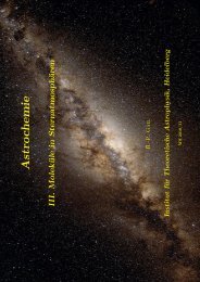
Fig. 1. Big Bang nucleosynthesis predictions for the abundances of light elements as a function of the baryon over photon ratio<br />
η or Ω b h 2 [156]. From Ref. [235].<br />
where L is the Liouville operator, <strong>and</strong> C is the collision operator, describing the interactions of the particle<br />
species considered.<br />
After some manipulation, the Boltzmann equation can be written as an equation for the particle number<br />
density n:<br />
dn<br />
dt + 3Hn=−〈σv〉(n2 − (n eq ) 2 ), (15)<br />
where σv is the total annihilation cross section multiplied by velocity, brackets denote thermal average,<br />
H is Hubble constant, <strong>and</strong> n eq is the number density at thermal equilibrium. For massive particles, i.e. in<br />
the non-relativistic limit, <strong>and</strong> in the Maxwell–Boltzmann approximation, one has<br />
( ) mT 3/2<br />
n eq = g e −m/T , (16)<br />
2π
288 G. Bertone et al. / Physics Reports 405 (2005) 279–390<br />
where m is the particle mass <strong>and</strong> T is the temperature. We next introduce the variables<br />
Y ≡ n s , Yeq ≡ neq<br />
, (17)<br />
s<br />
where s is the entropy density s=2π 2 g ∗ T 3 /45 <strong>and</strong> g ∗ counts the number of relativistic degrees of freedom.<br />
Using the conservation of entropy per co-moving volume (sa 3 =constant), it follows that ṅ + 3Hn= sẎ<br />
<strong>and</strong> Eq. (15) reads<br />
sẎ =−〈σv〉s 2 (Y 2 − (Y eq ) 2 ). (18)<br />
If we further introduce the variable x ≡ m/T , Eq. (18) can be expressed as<br />
dY<br />
dx =−〈σv〉s<br />
(<br />
Y 2 − (Y eq ) 2) . (19)<br />
Hx<br />
For heavy states, we can approximate 〈σv〉 with the non-relativistic expansion in powers of v 2<br />
〈σv〉=a + b〈v 2 〉+O(〈v 4 〉) ≈ a + 6b/x , (20)<br />
which leads to our final version of Eq. (19) in terms of the variable Δ = Y − Y eq :<br />
Δ ′ =−Y eq′ − f(x)Δ(2Y eq + Δ) , (21)<br />
where prime denotes d/dx <strong>and</strong><br />
√<br />
πg∗<br />
f(x)=<br />
45 mM Pl (a + 6b/x) x −2 . (22)<br />
Following Ref. [340] we introduce the quantity x F ≡ m/T F , where T F is the freeze-out temperature<br />
of the relic particle, <strong>and</strong> we notice that Eq. (21) can be solved analytically in the two extreme regions<br />
x>x F <strong>and</strong> x?x F ,<br />
Y eq′<br />
Δ =−<br />
2f(x)Y eq for x>x F , (23)<br />
Δ ′ =−f(x)Δ 2 for x?x F . (24)<br />
These regions correspond to long before freeze-out <strong>and</strong> long after freeze-out, respectively. Integrating the<br />
last equation between x F <strong>and</strong> ∞ <strong>and</strong> using Δ xF ?Δ ∞ , we can derive the value of Δ ∞ <strong>and</strong> arrive at<br />
Y −1<br />
∞<br />
= √<br />
πg∗<br />
45 M Pl mx −1<br />
F (a + 3b/x F ). (25)<br />
The present density of a generic relic, X, is simply given by ρ X =m X n X =m X s 0 Y ∞ , where s 0 =2889.2cm −3<br />
is the present entropy density (assuming three Dirac neutrino species). The relic density can finally be<br />
expressed in terms of the critical density (see Eq. (6))<br />
Ω X h 2 ≈ 1.07 × 10⁹ GeV −1<br />
M Pl<br />
x F 1<br />
√<br />
g∗ (a + 3b/x F ) , (26)<br />
where a <strong>and</strong> b are expressed in GeV −2 <strong>and</strong> g ∗ is evaluated at the freeze-out temperature. It is conventional<br />
to write the relic density in terms of the Hubble parameter, h = H 0 /100 km s −1 Mpc −1 .
G. Bertone et al. / Physics Reports 405 (2005) 279–390 289<br />
To estimate the relic density, one is thus left with the calculation of the annihilation cross sections (in<br />
all of the possible channels) <strong>and</strong> the extraction of the parameters a <strong>and</strong> b, which depend on the particle<br />
mass. The freeze-out temperature x F can be estimated through the iterative solution of the equation<br />
[ √ ]<br />
45 g mM Pl (a + 6b/x F )<br />
x F = ln c(c + 2)<br />
8 2π 3 , (27)<br />
g∗ 1/2 x 1/2<br />
F<br />
where c is a constant of order one determined by matching the late-time <strong>and</strong> early-time solutions.<br />
It is sometimes useful to perform an order-of-magnitude estimate using an approximate version of<br />
Eq. (26) [319]:<br />
Ω X h 2 ≈ 3 × 10⁻²⁷ cm 3 s −1<br />
. (28)<br />
〈σv〉<br />
We note that the approximation introduced in Eq. (20) is not always justified (see e.g. Ref. [319]).<br />
For example, Ref. [437] suggests a scenario where the presence of a scalar field in the early Universe<br />
could significantly affect the value of the relic density. Furthermore, a dramatic change in the relic density<br />
can be induced by resonance enhancements or the so-called coannihilations. We discuss the effects of<br />
coannihilations in the next section.<br />
1.5.2. Including coannihilations<br />
Following earlier works (see Ref. [103]), Griest <strong>and</strong> Seckel [279] noticed that if one or more particles<br />
have a mass similar to the relic particle <strong>and</strong> share a quantum number with it, the st<strong>and</strong>ard calculation of<br />
relic density fails.<br />
Let us consider N particles X i (i=1,...,N) with masses m i <strong>and</strong> internal degrees of freedom (statistical<br />
weights) g i . Also assume that m 1 m 2 ···m N−1 m N , <strong>and</strong> that the lightest particle is protected<br />
against decay thanks to some symmetry (i.e. R-parity or KK-parity, for neutralinos or Kaluza–Klein<br />
particles, respectively. See Section 3). We will also denote the lightest particle by X 1 .<br />
In this case, Eq. (15) becomes<br />
dn<br />
dt =−3Hn−<br />
N ∑<br />
i,j=1<br />
〈σ ij v ij 〉(n i n j − n eq<br />
i<br />
n eq<br />
j<br />
), (29)<br />
where n is the number density of the relic particle <strong>and</strong> n = ∑ N<br />
i=1 n i , due to the fact that the decay rate of<br />
particles, X i , other than the lightest is much faster than the age of the Universe. Here,<br />
σ ij = ∑ X<br />
σ(X i X j → X SM ) (30)<br />
is the total annihilation rate for X i X j annihilations into a st<strong>and</strong>ard model particle. Finally,<br />
√<br />
(p i · p j ) 2 − m 2 i m2 j<br />
v ij =<br />
(31)<br />
E i E j<br />
is the relative particle velocity, with p i <strong>and</strong> E i being the four-momentum <strong>and</strong> energy of particle i.
290 G. Bertone et al. / Physics Reports 405 (2005) 279–390<br />
The thermal average 〈σ ij v ij 〉 is defined with equilibrium distributions <strong>and</strong> is given by<br />
∫<br />
d 3 p i d 3 p j f i f j σ ij v ij<br />
〈σ ij v ij 〉= ∫<br />
d 3 p i d 3 , (32)<br />
p j f i f j<br />
where f i are distribution functions in the Maxwell–Boltzmann approximation.<br />
The scattering rate of supersymmetric particles off particles in the thermal background is much faster<br />
than their annihilation rate. We then obtain<br />
dn<br />
dt =−3Hn−〈σ effv〉(n 2 − n 2 eq ), (33)<br />
where<br />
〈σ eff v〉= ∑ ij<br />
〈σ ij v ij 〉 neq n eq<br />
i j<br />
n eq . (34)<br />
neq Edsjo <strong>and</strong> Gondolo [202] reformulated the thermal average into the more convenient expression<br />
∫ ∞<br />
0<br />
dp eff peff 2 〈σ eff v〉=<br />
W effK 1 ( √ s/T )<br />
m 4 1 T [∑ i g i/g 1 m 2 i /m2 1 K 2(m i /T) ] 2 , (35)<br />
where K i are the modified Bessel functions of the second kind <strong>and</strong> of order i. The quantity W eff is defined<br />
as<br />
W eff = ∑ p ij g i g j<br />
p<br />
ij 11 g1<br />
2 W ij = ∑ √<br />
[s − (m i − m j ) 2 ][s − (m i + m j ) 2 ] g i g j<br />
s(s − 4m 2 ij<br />
1 )<br />
g1<br />
2 W ij , (36)<br />
where W ij =4E i E j σ ij v ij <strong>and</strong> p ij is the momentum of the particle X i (or X j ) in the center-of-mass frame<br />
of the pair X i X j , <strong>and</strong> s = m 2 i + m2 j + 2E iE j − 2|p i ||p j | cos θ, with the usual meaning of the symbols.<br />
The details of coannihilations in the framework of supersymmetric models are well established (see e.g.<br />
the recent work of Edsjo et al. [206]), <strong>and</strong> numerical codes now exist including coannihilations with all<br />
supersymmetric particles, e.g. MicrOMEGAs [68] <strong>and</strong> the new version of DarkSusy [263,264], publicly<br />
released in 2004. The case of coannhilations with a light top squark, such as the one required for the<br />
realization of the electroweak baryogenesis mechanism, has been discussed in Ref. [55].<br />
1.6. Links with physics beyond the St<strong>and</strong>ard Model<br />
The concepts of <strong>dark</strong> energy <strong>and</strong> <strong>dark</strong> <strong>matter</strong> do not find an explanation in the framework of the St<strong>and</strong>ard<br />
Model of particle physics. Nor are they understood in any quantitative sense in terms of astrophysics.<br />
It is interesting that also in the realm of particle physics, <strong>evidence</strong> is accumulating for the existence of<br />
physics beyond the St<strong>and</strong>ard Model, based on theoretical <strong>and</strong> perhaps experimental arguments.<br />
On the experimental side, there is strong <strong>evidence</strong> for oscillations of atmospheric neutrinos (originating<br />
from electromagnetic cascades initiated by cosmic rays in the upper atmosphere) <strong>and</strong> solar neutrinos. The<br />
oscillation mechanism can be explained under the hypothesis that neutrinos do have mass, in contrast to<br />
the zero mass neutrinos of the St<strong>and</strong>ard Model (see Ref. [369] for a recent review).
G. Bertone et al. / Physics Reports 405 (2005) 279–390 291<br />
On the theoretical side, many issues make the St<strong>and</strong>ard Model unsatisfactory, for example the hierarchy<br />
problem, i.e. the enormous difference between the weak <strong>and</strong> Planck scales in the presence of the Higgs<br />
field (this will be discussed in some detail in Section 3.2.1), or the problem of unification addressing the<br />
question of whether there exists a unified description of all known forces, possibly including gravity.<br />
The list of problems could be much longer, <strong>and</strong> it is natural to conjecture that our St<strong>and</strong>ard Model is<br />
the low-energy limit of a more fundamental theory. Two examples of popular extensions of the St<strong>and</strong>ard<br />
Model include:<br />
• Supersymmetry. As a complete symmetry between fermions <strong>and</strong> bosons, supersymmetry’s theoretical<br />
appeal is very great [498]. So great, in fact, is this appeal, that it appears to many as a necessary<br />
ingredient of future extensions of the St<strong>and</strong>ard Model. Many interesting features make it attractive,<br />
including its role in underst<strong>and</strong>ing the fundamental distinction between bosons <strong>and</strong> fermions, <strong>and</strong> the<br />
problems of hierarchy <strong>and</strong> unification discussed above. Last, but not least, it provides an excellent<br />
<strong>dark</strong> <strong>matter</strong> c<strong>and</strong>idate in terms of its lightest stable particle, the neutralino. We will present the basics<br />
of supersymmetry <strong>and</strong> the properties of the neutralino in Section 3.2.<br />
• Extra dimensions. In the search of a fundamental theory with a unified description of all interactions,<br />
physicists developed theories with extra spatial dimensions, following an early idea of Kaluza [322],<br />
who extended to four the number of space dimensions to include electromagnetism into a “geometric”<br />
theory of gravitation. In theories with unified extra dimensions, in which all particles <strong>and</strong> fields of<br />
the St<strong>and</strong>ard Model can propagate in the extra dimensions, the lightest Kaluza–Klein particle, i.e. the<br />
lightest of all the states corresponding to the first excitations of the particles of the St<strong>and</strong>ard Model, is<br />
a viable <strong>dark</strong> <strong>matter</strong> c<strong>and</strong>idate, as we discuss in Section 3.3.<br />
Despite the fact that neutrinos are thought to be massive, they are essentially ruled out as <strong>dark</strong> <strong>matter</strong><br />
<strong>c<strong>and</strong>idates</strong> (see Section 3.1). Consequently, the St<strong>and</strong>ard Model does not provide a viable <strong>dark</strong> <strong>matter</strong><br />
c<strong>and</strong>idate. This is further supported by the fact that most of the <strong>dark</strong> <strong>matter</strong> is non-baryonic (see Section<br />
2.3). Dark <strong>matter</strong> is therefore a motivation to search for physics beyond the St<strong>and</strong>ard Model (others might<br />
say that this is <strong>evidence</strong> for physics beyond the St<strong>and</strong>ard Model).<br />
This is a typical example of the strong interplay between particle physics, theoretical physics, cosmology<br />
<strong>and</strong> astrophysics. From one side, theoretical particle physics stimulates the formulation of new<br />
theories predicting new particles that turn out to be excellent <strong>dark</strong> <strong>matter</strong> <strong>c<strong>and</strong>idates</strong>. On the other side,<br />
cosmological <strong>and</strong> astrophysical observations constrain the properties of such particles <strong>and</strong> consequently<br />
the parameters of the new theories.<br />
2. Evidence <strong>and</strong> distribution<br />
2.1. The galactic scale<br />
The most convincing <strong>and</strong> direct <strong>evidence</strong> for <strong>dark</strong> <strong>matter</strong> on galactic scales comes from the observations<br />
of the rotation curves of galaxies, namely the graph of circular velocities of stars <strong>and</strong> gas as a function<br />
of their distance from the galactic center.<br />
Rotation curves are usually obtained by combining observations of the 21 cm line with optical surface<br />
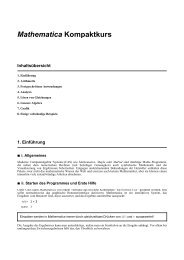
photometry. Observed rotation curves usually exhibit a characteristic flat behavior at large distances, i.e.<br />
out towards, <strong>and</strong> even far beyond, the edge of the visible disks (see a typical example in Fig. 2).
292 G. Bertone et al. / Physics Reports 405 (2005) 279–390<br />
Fig. 2. Rotation curve of NGC 6503. The dotted, dashed <strong>and</strong> dash–dotted lines are the contributions of gas, disk <strong>and</strong> <strong>dark</strong> <strong>matter</strong>,<br />
respectively. From Ref. [50].<br />
In Newtonian dynamics the circular velocity is expected to be<br />
√<br />
GM(r)<br />
v(r) =<br />
r<br />
, (37)<br />
where, as usual, M(r) ≡ 4π ∫ ρ(r)r 2 dr, <strong>and</strong> ρ(r) is the mass density profile, <strong>and</strong> should be falling<br />
∝ 1/ √ r beyond the optical disc. The fact that v(r) is approximately constant implies the existence of an<br />
halo with M(r) ∝ r <strong>and</strong> ρ ∝ 1/r 2 .<br />
Among the most interesting objects, from the point of view of the observation of rotation curves, are the<br />
so-called low surface brightness (LSB) galaxies, which are probably everywhere <strong>dark</strong> <strong>matter</strong> dominated,<br />
with the observed stellar populations making only a small contribution to rotation curves. Such a property<br />
is extremely important because it allows one to avoid the difficulties associated with the deprojection <strong>and</strong><br />
disentanglement of the <strong>dark</strong> <strong>and</strong> visible contributions to the rotation curves.<br />
Although there is a consensus about the shape of <strong>dark</strong> <strong>matter</strong> halos at large distances, it is unclear<br />
whether galaxies present cuspy or shallow profiles in their innermost regions, which is an issue of crucial<br />
importance for the effects we will be discussing in the following chapters.<br />
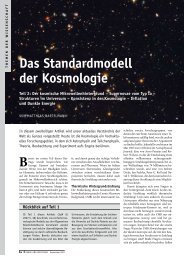
Using high-resolution data of 13 LSB galaxies, de Blok et al. [179] recently showed, that the distribution<br />
of inner slopes, i.e. the power-law indices of the density profile in the innermost part of the galaxies,<br />
suggests the presence of shallow, or even flat, cores (see Fig. 3). Furthermore, the highest values of the<br />
power-law index are obtained in correspondence to galaxies with the poorest resolution, as can be seen<br />
from the right panel of the same figure.<br />
Following Salucci <strong>and</strong> Borriello [439], rotation curves of both low <strong>and</strong> high surface luminosity galaxies<br />
appear to suggest a universal density profile, which can be expressed as the sum of an exponential<br />
thin stellar disk, <strong>and</strong> a spherical <strong>dark</strong> <strong>matter</strong> halo with a flat core of radius r 0 <strong>and</strong> density ρ 0 = 4.5 ×<br />
10 −2 (r 0 /kpc) −2/3 M ⊙ pc −3 (here, M ⊙ denotes a solar mass, 2 × 10 30 kg). In a similar way the analysis of<br />
Reed et al. [425] leads to the conclusion that simulated halos have significantly steeper density profiles<br />
than are inferred from observations.
G. Bertone et al. / Physics Reports 405 (2005) 279–390 293<br />
Fig. 3. Left panel:the distribution of inner slopes, α, of <strong>dark</strong> <strong>matter</strong> density profiles in LSB galaxies. The hatched (blank)<br />
histogram represents well-resolved (unresolved) galaxies. Right panel:the value of α as a function of the radius of the innermost<br />
point. From Ref. [179].<br />
Nevertheless, claims have been made in the literature about the possibility of reconciling these results<br />
with the steep profiles predicted by numerical simulations (see Section 2.4 for a discussion on the state<br />
of art of N-body simulations <strong>and</strong> for further discussions, see Refs. [179,427,483]). In particular, Hayashi<br />
et al. [291] have claimed consistency between most observations <strong>and</strong> their simulated profiles <strong>and</strong> have<br />
argued that the remaining discrepancies could be explained by taking into account the difference between<br />
the circular velocity <strong>and</strong> gas rotation speed, likely to arise in gaseous disks embedded within realistic,<br />
triaxial cold <strong>dark</strong> <strong>matter</strong> halos.<br />
Another area of contention is that of the <strong>dark</strong> <strong>matter</strong> content in the inner halos of massive disk galaxies.<br />
It has been argued that barred galaxies cannot contain substantial amounts of <strong>dark</strong> <strong>matter</strong> out to the<br />
outermost extent of the observed bars, otherwise the rapidly rotating bars would have slowed down due<br />
to dynamical friction on the <strong>dark</strong> <strong>matter</strong> [177,178]. One counterargument is the contention that bars may<br />
be dynamically young systems that formed by secular evolution of unstable cold disks <strong>and</strong> hence poor<br />
dynamical probes [158]. Another is that the slowing down of bars, perhaps in an earlier phase of the<br />
forming galaxy, actually heated the <strong>dark</strong> <strong>matter</strong> <strong>and</strong> generated a core.<br />
Despite the uncertainties of the slope in the innermost regions of galaxies, rotation curves of disk<br />
galaxies provide strong <strong>evidence</strong> for the existence of a spherical <strong>dark</strong> <strong>matter</strong> halo. The total amount of<br />
<strong>dark</strong> <strong>matter</strong> present is difficult to quantify, however, as we do not know to what distances halos extend.<br />
Additional <strong>evidence</strong> for <strong>dark</strong> <strong>matter</strong> at galactic scales comes from mass modelling of the detailed rotation<br />
curves, including spiral arm features. Submaximal disks are often, although not always, required [455].<br />
Some elliptical galaxies show <strong>evidence</strong> for <strong>dark</strong> <strong>matter</strong> via strong gravitational lensing [341]. X-ray<br />
<strong>evidence</strong> reveals the presence of extended atmospheres of hot gas that fill the <strong>dark</strong> halos of isolated<br />
ellipticals <strong>and</strong> whose hydrostatic support provides <strong>evidence</strong> for <strong>dark</strong> <strong>matter</strong>. In at least one case, an<br />
elliptical galaxy contains a cold gas disk whose HI rotation curve is flat out to about 5 half light radii.<br />
In contrast, however, planetary nebula studies to a similar distance for other ellipticals can be explained<br />
only with a constant mass-to-light ratio. There may be some <strong>dark</strong> <strong>matter</strong> in these cases, but its relative<br />
dominance does not appear to increase with increasing galactocentric distance. Rather, it is associated<br />
with the stellar distribution.
294 G. Bertone et al. / Physics Reports 405 (2005) 279–390<br />
Other arguments for <strong>dark</strong> <strong>matter</strong>, both on subgalactic <strong>and</strong> inter-galactic scales, also comes from a great<br />
variety of data. Without attempting to be complete, we cite among them:<br />
• Weak modulation of strong lensing around individual massive elliptical galaxies. This provides <strong>evidence</strong><br />
for substructure on scales of ∼ 10 6 M ⊙ [382,388].<br />
• The so-called Oort discrepancy in the disk of the Milky Way (see e.g. Ref. [51]). The argument follows<br />
an early suggestion of Oort, inferring the existence of unobserved <strong>matter</strong> from the inconsistency<br />
between the amount of stars, or other tracers in the solar neighborhood, <strong>and</strong> the gravitational potential<br />
implied by their distribution.<br />
• Weak gravitational lensing of distant galaxies by foreground structure (see, e.g. Ref. [299]).<br />
• The velocity dispersions of dwarf spheroidal galaxies which imply mass-to-light ratios larger than<br />
those observed in our “local” neighborhood. While the profiles of individual dwarfs show scatter,<br />
there is no doubt about the overall <strong>dark</strong> <strong>matter</strong> content (see Refs. [373,486]).<br />
• The velocity dispersions of spiral galaxy satellites which suggest the existence of <strong>dark</strong> halos around<br />
spiral galaxies, similar to our own, extending at galactocentric radii 200 kpc, i.e. well behind the<br />
optical disc. This applies in particular to the Milky Way, where both dwarf galaxy satellites <strong>and</strong> globular<br />
clusters probe the outer rotation curve (see Refs. [46,507]).<br />
2.2. The scale of galaxy clusters<br />
A cluster of galaxies gave the first hints of <strong>dark</strong> <strong>matter</strong> (in the modern sense). In 1933, Zwicky [510]<br />
inferred, from measurements of the velocity dispersion of galaxies in the Coma cluster, a mass-to-light<br />
ratio of around 400 solar masses per solar luminosity, thus exceeding the ratio in the solar neighborhood<br />
by two orders of magnitude. Today, most dynamical estimates [52,139,331] are consistent with a value<br />
Ω M ∼ 0.2–0.3 on cluster scales. A convenient calibration is Ω M = (M/L)/1000.<br />
The mass of a cluster can be determined via several methods, including application of the virial theorem<br />
to the observed distribution of radial velocities, by weak gravitational lensing, <strong>and</strong> by studying the profile<br />
of X-ray emission that traces the distribution of hot emitting gas in rich clusters.<br />
Consider the equation of hydrostatic equilibrium for a system with spherical symmetry<br />
1<br />
ρ<br />
dP<br />
dr<br />
=−a(r) , (38)<br />
where P, ρ, <strong>and</strong> a are, respectively, the pressure, density, <strong>and</strong> gravitational acceleration of the gas, at<br />
radius r. For an ideal gas, this can be rewritten in terms of the temperature, T, <strong>and</strong> the average molecular<br />
weight, μ ≈ 0.6,<br />
d log ρ<br />
d log r + d log T<br />
d log r =−r T<br />
( μmp<br />
k<br />
)<br />
a(r) , (39)<br />
where m p is the proton mass. The temperature of clusters is roughly constant outside of their cores <strong>and</strong><br />
the density profile of the observed gas at large radii roughly follows a power-law with an index between<br />
−2 <strong>and</strong> −1.5. We then find that the temperature should obey the relation<br />
( )( )<br />
Mr 1 Mpc<br />
kT ≈ (1.3 − 1.8) keV<br />
10 14 (40)<br />
M ⊙ r
G. Bertone et al. / Physics Reports 405 (2005) 279–390 295<br />
Fig. 4. Ch<strong>and</strong>ra X-ray (left) <strong>and</strong> Hubble Space Telescope Wide Field Planetary Camera 2 optical (right) images of Abell 2390<br />
(z = 0.230) <strong>and</strong> MS2137.3-2353 (z = 0.313). Note the clear gravitational arcs in the Hubble images. From Ref. [225].<br />
for the baryonic mass of a typical cluster, where M r is the mass enclosed within the radius r. The<br />
disparity between the temperature obtained using Eq. (40) <strong>and</strong> the corresponding observed temperature,<br />
T ≈ 10 keV, when M r is identified with the baryonic mass, suggests the existence of a substantial amount<br />
of <strong>dark</strong> <strong>matter</strong> in clusters.<br />
These conclusions can be checked against estimates from gravitational lensing data (see Fig. 4). Following<br />
Einstein’s theory of general relativity, light propagates along geodesics which deviate from straight<br />
lines when passing near intense gravitational fields. The distortion of the images of background objects<br />
due to the gravitational mass of a cluster can be used to infer the shape of the potential well <strong>and</strong> thus<br />
the mass of the cluster (see e.g. Ref. [477] for a spectacular demonstration of gravitational lensing in<br />
clusters).<br />
The fraction of baryons inside a cluster, crucial to disentangle the contributions of ordinary (visible) <strong>and</strong><br />
<strong>dark</strong> <strong>matter</strong>, can also be inferred through the so-called Sunyaev–Zel’dovich effect by which the cosmic<br />
microwave background (see Section 2.3) gets spectrally distorted through Compton scattering on hot<br />
electrons.<br />
Despite general agreement between <strong>dark</strong> <strong>matter</strong> density profiles at large radii <strong>and</strong> numerical simulations<br />
(see Section 2.4), it is unclear whether there is agreement with the predicted profiles in the cores of clusters.
296 G. Bertone et al. / Physics Reports 405 (2005) 279–390<br />
Gravitational lensing measurements appear to be in conflict with cuspy profiles, excluding at the 99%<br />
confidence level cusps with power-law indices of about −1 (see e.g. Ref. [440]).<br />
This argument is strengthened by use of radial arcs which probe the mass gradient, but is weakened if<br />
the cluster is not spherically symmetric. Indeed an asymmetry of a few percent allows the cluster profiles<br />
to be consistent with NFW. Moreover, recent Ch<strong>and</strong>ra observations of X-ray emission from Abell 2029<br />
suggest a full compatibility of <strong>dark</strong> <strong>matter</strong> distributions with cuspy profiles (see Ref. [358]). For a critique<br />
of gravitational lensing <strong>constraints</strong> on <strong>dark</strong> <strong>matter</strong> halo profiles, see Ref. [171].<br />
2.3. Cosmological scales<br />
We have seen in the previous sections that, on distance scales of the size of galaxies <strong>and</strong> clusters of<br />
galaxies, <strong>evidence</strong> of <strong>dark</strong> <strong>matter</strong> appears to be compelling. Despite this, the observations discussed do<br />
not allow us to determine the total amount of <strong>dark</strong> <strong>matter</strong> in the Universe. We discuss in this section how<br />
such information can be extracted from the analysis of the cosmic microwave background (CMB).<br />
Excellent introductions to CMB theory exist in the literature [312,313]. Here, we limit ourselves to a<br />
brief review of the implications of recent CMB data on the determination of cosmological parameters. In<br />
particular, we discuss the stringent <strong>constraints</strong> on the abundances of baryons <strong>and</strong> <strong>matter</strong> in the Universe<br />
placed by the Wilkinson microwave anisotropy probe (WMAP) data.<br />
The existence of background radiation originating from the propagation of photons in the early Universe<br />
(once they decoupled from <strong>matter</strong>) was predicted by George Gamow <strong>and</strong> his collaborators in 1948 <strong>and</strong><br />
inadvertently discovered byArno Penzias <strong>and</strong> Robert Wilson in 1965.After many decades of experimental<br />
effort, the CMB is known to be isotropic at the 10 −5 level <strong>and</strong> to follow with extraordinary precision the<br />
spectrum of a black body corresponding to a temperature T = 2.726 K.<br />
Today, the analysis of CMB anisotropies enables accurate testing of cosmological models <strong>and</strong> puts<br />
stringent <strong>constraints</strong> on cosmological parameters (Fig. 5).<br />
The observed temperature anisotropies in the sky are usually exp<strong>and</strong>ed as<br />
δT<br />
T (θ, ) = +∞ ∑<br />
+l<br />
∑<br />
l=2 m=−l<br />
a lm Y lm (θ, ) , (41)<br />
where Y lm (θ, ) are spherical harmonics. The variance C l of a lm is given by<br />
C l ≡〈|a lm | 2 〉≡ 1<br />
2l + 1<br />
l∑<br />
m=−l<br />
|a lm | 2 . (42)<br />
If the temperature fluctuations are assumed to be Gaussian, as appears to be the case, all of the information<br />
contained in CMB maps can be compressed into the power spectrum, essentially giving the behavior of<br />
C l as a function of l. Usually plotted is l(l + 1)C l /2π (see Fig. 6).<br />
The methodology, for extracting information from CMB anisotropy maps, is simple, at least in principle.<br />
Starting from a cosmological model with a fixed number of parameters (usually 6 or 7), the best-fit<br />
parameters are determined from the peak of the N-dimensional likelihood surface.<br />
From the analysis of the WMAP data alone, the following values are found for the abundance of baryons<br />
<strong>and</strong> <strong>matter</strong> in the Universe<br />
Ω b h 2 = 0.024 ± 0.001, Ω M h 2 = 0.14 ± 0.02 . (43)
G. Bertone et al. / Physics Reports 405 (2005) 279–390 297<br />
Fig. 5. CMB temperature fluctuations:a comparison between COBE <strong>and</strong> WMAP. Image from http://map.gsfc.nasa.gov/.<br />
Taking into account data from CMB experiments studying smaller scales (with respect to WMAP), such<br />
as ACBAR [348] <strong>and</strong> CBI [411], <strong>and</strong> astronomical measurements of the power spectrum from large scale<br />
structure (2dFGRS, see Ref. [414]) <strong>and</strong> the Lyman α forest (see e.g. Ref. [167]), the <strong>constraints</strong> become<br />
[457]<br />
Ω b h 2 = 0.0224 ± 0.0009 <strong>and</strong> Ω M h 2 = 0.135 +0.008<br />
−0.009 . (44)<br />
The value of Ω b h 2 thus obtained is consistent with predictions from Big Bang nucleosynthesis (e.g. [403])<br />
0.018 < Ω b h 2 < 0.023 . (45)<br />
Besides those provided by CMB studies, the most reliable cosmological measurements are probably<br />
those obtained by Sloan Digital Sky Survey (SDSS) team, which has recently measured the threedimensional<br />
power spectrum, P(k), using over 200,000 galaxies. An estimate of the cosmological<br />
parameters combining the SDSS <strong>and</strong> WMAP measurements can be found in Ref. [469].
298 G. Bertone et al. / Physics Reports 405 (2005) 279–390<br />
Fig. 6. The observed power spectrum of CMB anisotropies. From Ref. [470].<br />
2.4. N-body simulations<br />
Our underst<strong>and</strong>ing of large scale structure is still far from a satisfactory level. The description of the<br />
evolution of structures from seed inhomogeneities, i.e. primordial density fluctuations, is complicated by<br />
the action of many physical processes like gas dynamics, radiative cooling, photoionization, recombination<br />
<strong>and</strong> radiative transfer. Furthermore, any theoretical prediction has to be compared with the observed<br />
luminous Universe, i.e. with regions where dissipative effects are of crucial importance.<br />
The most widely adopted approach to the problem of large-scale structure formation involves the<br />
use of N-body simulations. The first simulation of interacting galaxies was performed by means of an<br />
analog optical computer (Holmberg 1941 [301]) using the flux from 37 light-bulbs, with photo-cells<br />
<strong>and</strong> galvanometers to measure <strong>and</strong> display the inverse square law of gravitational force. Modern, high<br />
resolution simulations make full use of the tremendous increase in computational power over the last few<br />
decades.<br />
The evolution of structure is often approximated with non-linear gravitational clustering from specified<br />
initial conditions of <strong>dark</strong> <strong>matter</strong> particles <strong>and</strong> can be refined by introducing the effects of gas dynamics,<br />
chemistry, radiative transfer <strong>and</strong> other astrophysical processes. The reliability of an N-body simulation is<br />
measured by its mass <strong>and</strong> length resolution. The mass resolution is specified by the mass of the smallest<br />
(“elementary”) particle considered, being the scale below which fluctuations become negligible. Length<br />
resolution is limited by the so-called softening scale, introduced to avoid infinities in the gravitational<br />
force when elementary particles collide.<br />
Recent N-body simulations suggest the existence of a universal <strong>dark</strong> <strong>matter</strong> profile, with the same<br />
shape for all masses, epochs <strong>and</strong> input power spectra [393]. The usual parametrisation for a <strong>dark</strong> <strong>matter</strong>
G. Bertone et al. / Physics Reports 405 (2005) 279–390 299<br />
Table 2<br />
Parameters of some widely used profile models for the <strong>dark</strong> <strong>matter</strong> density in galaxies (See Eq. (46)). Values of R can vary from<br />
system to system<br />
α β γ R (kpc)<br />
Kra 2.0 3.0 0.4 10.0<br />
NFW 1.0 3.0 1.0 20.0<br />
Moore 1.5 3.0 1.5 28.0<br />
Iso 2.0 2.0 0 3.5<br />
halo density is<br />
ρ(r) =<br />
ρ 0<br />
(r/R) γ [1 + (r/R) α . (46)<br />
(β−γ)/α<br />
]<br />
Various groups have ended up with different results for the spectral shape in the innermost regions of<br />
galaxies <strong>and</strong> galaxy clusters. In particular, several groups have failed to reproduce the initial results of<br />
Navarro, Frenk <strong>and</strong> White [393], which find a value for the power-law index in the innermost part of<br />
galactic halos of γ = 1. In Table 2, we give the values of the parameters (α, β, γ) for some of the most<br />
widely used profile models, namely the Kravtsov et al. (Kra, [346]), Navarro, Frenk <strong>and</strong> White (NFW,<br />
[393]), Moore et al. (Moore, [384]) <strong>and</strong> modified isothermal (Iso, e.g. Ref. [80]) profiles.<br />
Although it is definitely clear that the slope of the density profile should increase as one moves from<br />
the center of a galaxy to the outer regions, the precise value of the power-law index in the innermost<br />
galactic regions is still under debate. Attention should be paid when comparing the results of different<br />
groups, as they are often based on a single simulation, sometimes at very different length scales.<br />
Taylor <strong>and</strong> Navarro [394,468] studied the behavior of the phase-space density (defined as the ratio of<br />
spatial density to velocity dispersion cubed, ρ/σ 3 ) as a function of the radius, finding excellent agreement<br />
with a power-law extending over several decades in radius, <strong>and</strong> also with the self-similar solution derived<br />
by Bertschinger [96] for secondary infall onto a spherical perturbation. The final result of their analysis<br />
is a “critical” profile, following a NFW profile in the outer regions, but with a central slope converging<br />
to the value γ TN = 0.75, instead of γ NFW = 1.<br />
The most recent numerical simulations (see Navarro et al. [395], Reed et al. [425] <strong>and</strong> Fukushige et al.<br />
[242]) appear to agree on a new paradigm, suggesting that density profiles do not converge to any specific<br />
power-law at small radii. The logarithmic slope of the profile continuously flattens when moving toward<br />
the galactic center. The slope at the innermost resolved radius varies between 1 <strong>and</strong> 1.5, i.e. between the<br />
predictions of the NFW <strong>and</strong> Moore profiles. It is important to keep in mind that predictions made adopting<br />
such profiles probably overestimate the density near the Galactic center <strong>and</strong> should be used cautiously.<br />
Recently, Prada et al. [421] have suggested that the effects of adiabatic compression on the <strong>dark</strong> <strong>matter</strong><br />
profile near the Galactic center could play an important role, possibly enhancing the <strong>dark</strong> <strong>matter</strong> density<br />
by an order of magnitude in the inner parsecs of the Milky Way.<br />
The extrapolations of cuspy profiles at small radii have appeared in the past (<strong>and</strong> still appear to some) to<br />
be in disagreement with the flat cores observed in astrophysical systems, such as low surface brightness<br />
galaxies mentioned earlier. Such discrepancies prompted proposals to modify the properties of <strong>dark</strong><br />
<strong>matter</strong> particles, to make them self-interacting, warm, etc. Most of such proposals appear to create more<br />
problems than they solve <strong>and</strong> will not be discussed here.
300 G. Bertone et al. / Physics Reports 405 (2005) 279–390<br />
Today, the situation appear less problematic, in particular after the analysis of Hayashi et al. [291].<br />
Our approach, given the uncertainties regarding observed <strong>and</strong> simulated halo profiles, will be to consider<br />
the central slope of the galactic density profile as a free parameter <strong>and</strong> discuss the prospects of indirect<br />
detection of <strong>dark</strong> <strong>matter</strong> for the different models proposed in literature.<br />
2.5. The case of the Milky Way<br />
Since the Milky Way is prototypical of the galaxies that contribute most to the cosmic luminosity<br />
density, it is natural to ask how the results discussed in the previous section compare with the wide range<br />
of observational data available for our galaxy.<br />
One way to probe the nature of <strong>matter</strong> in our neighborhood is to study microlensing events in the<br />
direction of the galactic center. In fact, such events can only be due to compact objects, acting as lenses<br />
of background sources, <strong>and</strong> it is commonly believed that <strong>dark</strong> <strong>matter</strong> is simply too weakly interacting to<br />
clump on small scales. 2<br />
Binney <strong>and</strong> Evans (BE) [104] recently showed that the number of observed microlensing events implies<br />
an amount of baryonic <strong>matter</strong> within the Solar circle greater than about 3.9 × 10 10 M ⊙ . Coupling this<br />
result with estimates of the local <strong>dark</strong> <strong>matter</strong> density, they exclude cuspy profiles with power-law index<br />
γ0.3.<br />
Nevertheless, Klypin, Zhao <strong>and</strong> Somerville (KZS) [334] find a good agreement between NFW profiles<br />
(γ = 1) <strong>and</strong> observational data for our galaxy <strong>and</strong> M31. The main difference between these analyses is the<br />
value of the microlensing optical depth towards the Galactic center used. Observations of this quantity<br />
disagree by a factor of ∼ 3 <strong>and</strong> a low value within this range permits the presence of a <strong>dark</strong> <strong>matter</strong><br />
cusp. Another difference arises from the modeling of the galaxy:KZS claim to have taken into account<br />
dynamical effects neglected by BE <strong>and</strong> to have a “more realistic” description of the galactic bar.<br />
An important addition is adiabatic compression of the <strong>dark</strong> <strong>matter</strong> by baryonic dissipation. This results<br />
in a <strong>dark</strong> <strong>matter</strong> density that is enhanced in the core by an order of magnitude. This result can be reconciled<br />
with modelling of the rotation curve if the lower value of the microlensing optical depth found by the<br />
EROS collaboration is used rather than that of the MACHO collaboration. In the latter case, little <strong>dark</strong><br />
<strong>matter</strong> is allowed in the central few kpc. The microlensing result constrains the stellar contribution to the<br />
inner rotation curve, <strong>and</strong> hence to the total allowed density.<br />
2.5.1. The Galactic center<br />
The <strong>dark</strong> <strong>matter</strong> profile in the inner region of the Milky Way is even more uncertain. Observations of<br />
the velocity dispersion of high proper motion stars suggest the existence of a Super Massive Black Hole<br />
(SMBH) lying at the center of our galaxy, with a mass, M SMBH ≈ 2.6 × 10 6 M ⊙ [252]. 3<br />
Recently, near-infrared high-resolution imaging <strong>and</strong> spectroscopic observations of individual stars, as<br />
close as a few light days from the galactic center, were carried out at Keck [251] <strong>and</strong> ESO/VLT telescopes<br />
(see Ref. [445], for an excellent <strong>and</strong> updated discussion of the stellar dynamics in the galactic center,<br />
2 It was noticed by Berezinsky et al. [76] that if microlensing was due to neutralino stars (see the definition of “neutralino”<br />
in the chapter on <strong>dark</strong> <strong>matter</strong> <strong>c<strong>and</strong>idates</strong>), i.e. self-gravitating systems of <strong>dark</strong> <strong>matter</strong> particles, then the gamma-ray radiation<br />
originated by annihilations in these object would exceed the observed emission.<br />
3 The existence of a SMBH at the center of the galaxy is not surprising. There is, in fact, mounting <strong>evidence</strong> for the existence<br />
of 10 6 –10 8 M ⊙ black holes in the centers of most galaxies with mass amounting to approximately 0.1% of the stellar spheroid<br />
(see, e.g. Ref. [342]).
G. Bertone et al. / Physics Reports 405 (2005) 279–390 301<br />
Fig. 7. The mass distribution in the galactic center, as derived by different observations, down to a 10 −4 pc scale. Lines represent<br />
fits under different assumptions, as specified by the text in the figure. In particular, the solid line is the overall best fit model:<br />
a2.87 ± 0.15 × 10 6 M ⊙ central object, plus a stellar cluster distributed with a power-law of index 1.8. For more details see<br />
Ref. [445].<br />
based on the most recent observations at ESO/VLT). The analysis of the orbital parameters of such stars<br />
suggest that the mass of the SMBH could possibly be a factor of two larger with respect to the above<br />
cited estimate from the velocity dispersion. In Fig. 7 we show a plot of the enclosed mass as a function<br />
of the galactocentric distance, along with a best-fit curve, which corresponds to a <strong>dark</strong> object with a mass<br />
of 2.87 ± 0.15 × 10 6 M ⊙ .<br />
It has long been argued (see e.g. Peebles, Ref. [412]) that if a SMBH exists at the galactic center, the<br />
process of adiabatic accretion of <strong>dark</strong> <strong>matter</strong> on it would produce a “spike” in the <strong>dark</strong> <strong>matter</strong> density<br />
profile. Gondolo <strong>and</strong> Silk [261] have recently applied such a process to study the enhancement of the<br />
annihilation signal from the galactic center.<br />
If we consider an initial power-law type profile of index γ, similar to those discussed in Section 2.4,<br />
the corresponding <strong>dark</strong> <strong>matter</strong> profile, ρ ′ (r), after this accretion process is, following Ref. [261],<br />
[ ( ) ]<br />
M<br />
3−γ γsp −γ ( ) D γsp<br />
ρ ′ = α γ<br />
ρ D D 3 ρ D g(r) , (47)<br />
r<br />
where γ sp = (9 − 2γ)/(4 − γ), D ≃ 8 kpc is the solar distance from the Galactic center <strong>and</strong> ρ D ≃<br />
0.3 GeV/c 2 /cm 3 is the density in the solar neighborhood. The factors α γ <strong>and</strong> g γ (r) cannot be determined<br />
analytically (for approximate expressions <strong>and</strong> numerical values see Ref. [261]). Eq. (47) is only valid<br />
in a central region of size R sp = α γ D(M/ρ D D 3 ) 1/(3−γ) , where the central black hole dominates the<br />
gravitational potential.<br />
It is easy to underst<strong>and</strong> the basics of adiabatic accretion under the assumptions of circular orbits.<br />
Assuming an initial power-law distribution, ρ ∝ r −γ , <strong>and</strong> a final distribution, ρ ∝ r −γ sp, the equations of<br />
conservation of mass <strong>and</strong> angular momentum can be expressed, respectively, as<br />
ρ i r 2 i dr i = ρ f r 2 f dr f (48)
302 G. Bertone et al. / Physics Reports 405 (2005) 279–390<br />
<strong>and</strong><br />
r i M i (r) = r f M f (r) ≈ r f M BH , (49)<br />
which imply, respectively,<br />
<strong>and</strong><br />
r i ∝ r (3−γ sp)/(3−γ)<br />
f<br />
(50)<br />
r i ∝ r 1/(4−γ)<br />
f<br />
. (51)<br />
The final distribution will thus have a power-law index<br />
γ sp = 9 − 2γ<br />
4 − γ , (52)<br />
which assumes values in the range of 2.25–2.5 as γ varies in the interval of 0 to 2.<br />
If we take into account the annihilation of <strong>dark</strong> <strong>matter</strong> particles, the density cannot grow to arbitrarily<br />
high values, the maximal density being fixed by the value<br />
ρ core =<br />
m , (53)<br />
σvt BH<br />
where t BH ≈ 10 10 yr is the age of the central black hole. The final profile, resulting from the adiabatic<br />
accretion of annihilating <strong>dark</strong> <strong>matter</strong> on a massive black hole is<br />
ρ dm (r) =<br />
ρ′ (r)ρ core<br />
ρ ′ (54)<br />
(r) + ρ core<br />
following a power-law for large values of r, <strong>and</strong> with a flat core of density, ρ core , <strong>and</strong> dimension,<br />
( )<br />
ρ(Rsp ) (1/γsp )<br />
R core = R sp . (55)<br />
ρ core<br />
We will use these equations when discussing the prospects for indirect detection of <strong>dark</strong> <strong>matter</strong> in the<br />
presence of a spike. We recall, nevertheless, that they have been derived under the simplifying assumption<br />
that the SMBH formed at a position coinciding exactly with the center of the galactic potential well, <strong>and</strong><br />
neglecting all dynamical effects.<br />
It was shown by Ullio et al. [481] that if the black hole forms from a low-mass seed, then its spiral-in<br />
to reach the exact center of the galaxy could take a length of time longer than the age of the galaxy. If,<br />
conversely, the seed black hole is massive, the back-reaction to the spiral-in of the black hole leads to<br />
the formation of a weak-density cusp, with ρ ∝ r −0.5 . Fig. 8 shows the modification of an NFW <strong>dark</strong><br />
<strong>matter</strong> profile due to the off-center formation of the seed black hole. The solution found by Gondolo <strong>and</strong><br />
Silk would be indistinguishable from the case of an initial light seed of roughly 10 −2 M SMBH , starting its<br />
growth very near to the galactic center.<br />
The spike could also be destroyed by hierarchical mergers, as discussed by Merritt et al. [381], but<br />
such mergers are unlikely to have occurred in the recent history of the Milky Way. What can be stated<br />
with considerable confidence is that the Milky Way galaxy underwent one significant merger about 12<br />
billion years ago. This resulted in the formation of the bulge, <strong>and</strong> therefore presumably of the SMBH,
G. Bertone et al. / Physics Reports 405 (2005) 279–390 303<br />
10 16 10 -8 10 -7 10 -6 10 -5 10 -4 10 -3 10 -2 10 -1 1 10<br />
10 14<br />
10 -4 M BH<br />
/ 10 -5 M BH<br />
initial profile<br />
ρ [ M pc -3 ]<br />
10 12 10 -3 M BH<br />
10 10<br />
10 -2 M BH<br />
10 8<br />
10 6<br />
10 -1 M BH<br />
10 4<br />
MBH S spiral-in +<br />
approx. adiabatic growth<br />
ρ core<br />
10 2<br />
1<br />
10 -2<br />
M S BH = M BH<br />
NFW profile<br />
10 -4<br />
r [ kpc ]<br />
Fig. 8. Modification of an NFW profile due to the off-center formation of a black-hole seed of mass MBH S , its spiral-in the center<br />
of the <strong>dark</strong> <strong>matter</strong> system <strong>and</strong> its adiabatic growth to the present-day mass, M SMBH (called M SM in the figure). From Ref. [481].<br />
<strong>and</strong> of the thick disk. The chemical <strong>evidence</strong> for a unique merger origin in the case of our Milky Way’s<br />
thick disk is compelling [254,500], as the continuity between thin disk, thick disk, <strong>and</strong> bulge would have<br />
been destroyed had anything significant happened more recently in the way of a merger (see also the<br />
discussion of Bertone et al. [92]).<br />
Furthermore, the scattering of <strong>dark</strong> <strong>matter</strong> particles by stars in the dense stellar cusp observed around<br />
the SMBH could substantially lower the <strong>dark</strong> <strong>matter</strong> density near the Galactic center over 10 10 years, due<br />
both to kinetic heating, <strong>and</strong> to capture of <strong>dark</strong> <strong>matter</strong> particles by the SMBH [380].<br />
The existence of such spikes would produce a dramatic enhancement of the annihilation radiation from<br />
the galactic center. The implications for indirect detection of <strong>dark</strong> <strong>matter</strong> particles have been discussed<br />
in Refs. [91,92,261,262].<br />
2.5.2. The local density<br />
Very important to the prospects for direct <strong>and</strong> indirect detection is the density of <strong>dark</strong> <strong>matter</strong> in the<br />
region of our solar system. Although this quantity is considerably more well known than the density near<br />
the galactic center, there are still uncertainties associated with the local density, which we will discuss<br />
here.<br />
The local density of <strong>dark</strong> <strong>matter</strong> is determined by observing the rotation curves of the Milky Way. This<br />
is somewhat difficult to do from our location within the galaxy. Furthermore, rotation curves measure<br />
the total mass within an orbit, thus the density distributions of the galactic bulge <strong>and</strong> disk are needed to<br />
accurately calculate the <strong>dark</strong> <strong>matter</strong> profile.
304 G. Bertone et al. / Physics Reports 405 (2005) 279–390<br />
0.8<br />
0.7<br />
0.6<br />
local halo density ρ 0<br />
0.5<br />
0.4<br />
0.3<br />
0.2<br />
0.1<br />
R 0 = 8.5 kpc<br />
R 0 = 7.1 kpc<br />
0<br />
1 10 10 2<br />
core radius a (kpc)<br />
Fig. 9. The range of local <strong>dark</strong> <strong>matter</strong> densities acceptable with observations of rotation curves for a variety of halo profiles <strong>and</strong><br />
galactocentric distances. Densities in the range of 0.2–0.8 GeV/cm 3 are shown to be acceptable. From Ref. [80].<br />
Ka<br />
Kb<br />
NFW<br />
Sp<br />
In addition to the local density, the velocity distribution of <strong>dark</strong> <strong>matter</strong> in the local region is needed to<br />
accurately calculate direct <strong>and</strong> indirect detection rates. This is also best inferred from observed rotation<br />
curves.<br />
Different groups have come to somewhat different conclusions regarding the local density <strong>and</strong> velocity<br />
distribution of <strong>dark</strong> <strong>matter</strong>. For example, Bahcall et al. finds a best-fit value of ρ 0 = 0.34 GeV/cm 3 [53],<br />
Caldwell <strong>and</strong> Ostriker find ρ 0 = 0.23 GeV/cm 3 [136] while Turner calculates ρ 0 = 0.3–0.6 GeV/cm 3<br />
[473]. InFig. 9 we show the range of local <strong>dark</strong> <strong>matter</strong> densities found to be acceptable by Bergstrom<br />
et al. [80] for various choices of halo profile <strong>and</strong> galactocentric distance. They find local <strong>dark</strong> <strong>matter</strong><br />
densities acceptable in the range of about 0.2–0.8 GeV/cm 3 .<br />
The velocity distribution of <strong>dark</strong> <strong>matter</strong> is typically described only by its average velocity, ¯v=〈v 2 〉 1/2 ∼ =<br />
270 km/s.<br />
For more discussion on the local <strong>dark</strong> <strong>matter</strong> distribution, see Section 2.4 of Ref. [319].<br />
3. C<strong>and</strong>idates<br />
As we have seen in the previous section, the <strong>evidence</strong> for non-baryonic <strong>dark</strong> <strong>matter</strong> is compelling at<br />
all observed astrophysical scales. It is therefore natural to ask what is the <strong>dark</strong> <strong>matter</strong> made of ? In this<br />
section, we present some of the <strong>c<strong>and</strong>idates</strong> discussed in the literature, <strong>and</strong> focus our attention especially<br />
on two popular <strong>c<strong>and</strong>idates</strong>:the supersymmetric neutralino, probably the most widely studied c<strong>and</strong>idate,<br />
<strong>and</strong> the B (1) particle, the first Kaluza–Klein excitation of the B boson in theories with universal extra<br />
dimensions. We will also briefly discuss “superheavy” <strong>c<strong>and</strong>idates</strong>, also referred to as wimpzillas.
3.1. The non-baryonic c<strong>and</strong>idate zoo<br />
G. Bertone et al. / Physics Reports 405 (2005) 279–390 305<br />
There is no shortage of <strong>c<strong>and</strong>idates</strong> for non-baryonic <strong>dark</strong> <strong>matter</strong>. In this section we briefly describe<br />
some of these <strong>c<strong>and</strong>idates</strong>.<br />
• St<strong>and</strong>ard Model neutrinos<br />
Neutrinos have been considered, until recently, excellent <strong>dark</strong> <strong>matter</strong> <strong>c<strong>and</strong>idates</strong> for their “undisputed<br />
virtue of being known to exist” [86]. However, a simple calculation shows that, if we call m i the mass<br />
of the ith neutrino, their total relic density is predicted to be<br />
Ω ν h 2 =<br />
3∑<br />
i=1<br />
m i<br />
93 eV . (56)<br />
The best laboratory constraint on neutrino masses comes from tritium β-decay experiments at Troitsk<br />
<strong>and</strong> Mainz [496], pointing to the following upper limit on the neutrino mass:<br />
m ν < 2.05 eV (95% C.L.) , (57)<br />
while next-generation experiments are expected to reach a sensitivity of approximately 0.2 eV (see<br />
Ref. [496] <strong>and</strong> references therein). The above upper limit applies to all three mass eigenvalues [73],<br />
since the mass differences among them must be very small to explain solar (Δm 2 ≈ 7 × 10 −5 eV 2 )<br />
<strong>and</strong> atmospheric (Δm 2 ≈ 3 × 10 −3 eV 2 ) neutrino anomalies (see e.g. Ref. [265]). This implies an<br />
upper bound on the total neutrino relic density of<br />
Ω ν h 2 0.07 , (58)<br />
which means that neutrinos are simply not abundant enough to be the dominant component of <strong>dark</strong><br />
<strong>matter</strong>. A more stringent constraint on the neutrino relic density comes from the analysis of CMB<br />
anisotropies, combined with large-scale structure data, suggesting Ω ν h 2 < 0.0067 (95% confidence<br />
limit). For three degenerate neutrino species this implies m ν < 0.23 eV. If extra neutrino interactions<br />
are allowed, e.g., the coupling of neutrinos to a light boson, the neutrino mass limits arising from large<br />
scale structure can be evaded [74].<br />
Being relativistic collisionless particles, neutrinos erase (moving from high to low density regions)<br />
fluctuations below a scale of ∼ 40 Mpc (m ν /30 eV), called the free-streaming length [122]. This would<br />
imply a top–down formation history of structure in the Universe, where big structures form first. The<br />
fact that our galaxy appears to be older than the Local Group [413], <strong>and</strong> the discrepancy between the<br />
predicted late formation of galaxies, at redshift z1, against observations of galaxies around z>4<br />
[123], is a further argument against neutrinos as a viable <strong>dark</strong> <strong>matter</strong> c<strong>and</strong>idate.<br />
• Sterile neutrinos<br />
These hypothetical particles are similar to St<strong>and</strong>ard Model neutrinos, but without St<strong>and</strong>ard Model weak<br />
interactions, apart from mixing. They were proposed as <strong>dark</strong> <strong>matter</strong> <strong>c<strong>and</strong>idates</strong> in 1993 by Dodelson<br />
<strong>and</strong> Widrow [191]. Stringent cosmological <strong>and</strong> astrophysical <strong>constraints</strong> on sterile neutrinos come<br />
from the analysis of their cosmological abundance <strong>and</strong> the study of their decay products (see Ref. [1]<br />
<strong>and</strong> references therein).<br />
Light neutrinos, with masses below a few keV, would be ruled out as <strong>dark</strong> <strong>matter</strong> <strong>c<strong>and</strong>idates</strong>. In fact,<br />
if the WMAP result for the reionization optical depth is correct, then <strong>dark</strong> <strong>matter</strong> structures were in
306 G. Bertone et al. / Physics Reports 405 (2005) 279–390<br />
place to form massive stars prior to redshift z>20, which is simply not possible if the <strong>dark</strong> <strong>matter</strong><br />
particle mass is smaller than ∼ 10 keV [504]. An alternative explanation for the WMAP optical depth<br />
is reionization by decaying particles, such as sterile neutrinos (see Ref.[287] <strong>and</strong> references therein).<br />
Sterile neutrinos could also be cold <strong>dark</strong> <strong>matter</strong>, if there is a very small lepton asymmetry, in which<br />
case they are produced resonantly with a non-thermal spectrum [448].<br />
• Axions<br />
Introduced in an attempt to solve the problem of CP violation in particle physics, axions have also<br />
often been discussed as a <strong>dark</strong> <strong>matter</strong> c<strong>and</strong>idate.<br />
Laboratory searches, stellar cooling <strong>and</strong> the dynamics of supernova 1987A constrain axions to be very<br />
light (0.01 eV). Furthermore, they are expected to be extremely weakly interacting with ordinary<br />
particles, which implies that they were not in thermal equilibrium in the early universe.<br />
The calculation of the axion relic density is uncertain, <strong>and</strong> depends on the assumptions made regarding<br />
the production mechanism. Nevertheless, it is possible to find an acceptable range where axions satisfy<br />
all present-day <strong>constraints</strong> <strong>and</strong> represent a possible <strong>dark</strong> <strong>matter</strong> c<strong>and</strong>idate (see e.g. Ref. [428]).<br />
• Supersymmetric <strong>c<strong>and</strong>idates</strong><br />
◦ Neutralinos<br />
Neutralinos in models of R-parity conserving supersymmetry are by far the most widely studied<br />
<strong>dark</strong> <strong>matter</strong> <strong>c<strong>and</strong>idates</strong>. We devote Section 3.2 to their presentation.<br />
◦ Sneutrinos<br />
The superpartners of the St<strong>and</strong>ard Model neutrinos in supersymmetric models have long been<br />
considered as <strong>dark</strong> <strong>matter</strong> <strong>c<strong>and</strong>idates</strong>. It has been shown that sneutrinos will have a cosmologically<br />
interesting relic density if their mass is in the range of 550–2300 GeV. However, the scattering<br />
cross section of a sneutrino with nucleons is easily calculated <strong>and</strong> is much larger than the limits<br />
found by direct <strong>dark</strong> <strong>matter</strong> detection experiments [226].<br />
◦ Gravitinos<br />
Gravitinos are the superpartners of the graviton in supersymmetric models. In some supersymmetric<br />
scenarios, gauge mediated supersymmetry for example, gravitinos can be the lightest supersymmetric<br />
particle <strong>and</strong> be stable. Gravitinos are thus very strongly theoretically motivated. With<br />
only gravitational interactions, however, gravitinos are very difficult to observe [234].<br />
It has been known for some time that long livedgravitinos can pose problems for cosmology<br />
[214,216,390,409,494,505]. In particular, their presence can destroy the abundances of primordial<br />
light elements in some scenarios [170,219,233,385]. Gravitinos may also be overproduced in the<br />
early universe if the temperature of the reheating epoch is not sufficiently low [385]. In some<br />
scenarios, however, these problems can be circumvented [132,152,249].<br />
◦ Axinos<br />
Axinos, the superpartner of the axion, were believed until recently to only be capable of acting as<br />
a warm, or hot, <strong>dark</strong> <strong>matter</strong> c<strong>and</strong>idate [124,268]. It has been shown, however, that for quite low<br />
reheating temperatures, cold axino <strong>dark</strong> <strong>matter</strong> may be possible [164–166,366]. In many ways,<br />
axinos <strong>and</strong> gravitinos share similar phenomenological properties.<br />
• Light scalar <strong>dark</strong> <strong>matter</strong><br />
Considering fermionic <strong>dark</strong> <strong>matter</strong> <strong>c<strong>and</strong>idates</strong> with st<strong>and</strong>ard Fermi interactions, Lee <strong>and</strong> Weinberg<br />
concluded that relic density arguments preclude such a WIMP with a mass less than a few GeV [355]
G. Bertone et al. / Physics Reports 405 (2005) 279–390 307<br />
(see also Hut 1977 [314]). If the <strong>dark</strong> <strong>matter</strong> is made up of other types of particles, however, this limit<br />
could be evaded. For example, a 1–100 MeV scalar c<strong>and</strong>idate has been proposed [117,118].<br />
Such a c<strong>and</strong>idate, although somewhat ad hoc from a particle physics perspective, has recently become<br />
experimentally motivated. In Ref. [120], it has been suggested that the 511 keV gamma-ray line<br />
emission observed by the INTEGRAL satellite from the galactic bulge could be the product of light<br />
<strong>dark</strong> <strong>matter</strong> particles annihilating into positrons which then annihilate producing the observed gammaray<br />
line. To confirm this hypothesis, more tests are needed. In particular, a similar signature could be<br />
expected from dwarf spheroidal galaxies [304].<br />
Very recently, light decaying <strong>dark</strong> <strong>matter</strong> particles such as axinos with R-parity violation [311] or<br />
sterile neutrinos [416] have been suggested as the source of the observed 511 keV emission.<br />
• Dark <strong>matter</strong> from little Higgs models<br />
As an alternative mechanism (to supersymmetry) to stabilize the weak scale, the so-called “little<br />
Higgs” models have been proposed <strong>and</strong> developed [38–41]. In these models, the St<strong>and</strong>ard Model<br />
Higgs is a pseudo-Goldstone boson with its mass protected by approximate non-linear global symmetries.<br />
The divergences to the Higgs mass which remain are present only at the two-loop level<br />
<strong>and</strong>, therefore, the weak scale can be stabilized in an effective field theory which is valid up to<br />
∼ 10 TeV. Recall that in supersymmetry, the divergences to the Higgs mass are exactly cancelled at all<br />
orders.<br />
At least two varieties of little Higgs models have been shown to contain possible <strong>dark</strong> <strong>matter</strong> <strong>c<strong>and</strong>idates</strong>.<br />
One of these classes of models, called “theory space” little Higgs models, provide a possibly stable,<br />
scalar particle which can provide the measured density of <strong>dark</strong> <strong>matter</strong> [110]. In Ref. [105], the detection<br />
prospects for such a c<strong>and</strong>idate were found to be notdissimilar to WIMPs predicted in models of<br />
supersymmetry or universal extra dimensions.<br />
Cheng <strong>and</strong> Low [147] have developed another variety of little Higgs model, motivated by the problem of<br />
the hierarchy between the electroweak scale <strong>and</strong> the masses of new particles constrained by electroweak<br />
precision measurements. They solve this problem by introducing a new symmetry at the TeV scale<br />
which results in the existence of a stable WIMP c<strong>and</strong>idate with a ∼ TeV mass.<br />
For a potential <strong>dark</strong> <strong>matter</strong> c<strong>and</strong>idate from a little Higgs model to be stable, we must assume that the<br />
discrete symmetry which protects it from decay is fundamental <strong>and</strong> is not broken by the operators in<br />
the UV completion.<br />
• Kaluza–Klein states<br />
Kaluza–Klein excitations of St<strong>and</strong>ard Model fields which appear in models of universal extra dimensions<br />
have also been discussed a great deal recently as a c<strong>and</strong>idate for <strong>dark</strong> <strong>matter</strong>. They are discussed<br />
in Section 3.3. Additionally, a <strong>dark</strong> <strong>matter</strong> c<strong>and</strong>idate has been proposed in the framework of “warped”<br />
universal extra-dimensions:an exotic particle with gauge quantum numbers of a right-h<strong>and</strong>ed neutrino,<br />
but carrying fractional baryon-number [15].<br />
• Superheavy <strong>dark</strong> <strong>matter</strong><br />
Superheavy <strong>dark</strong> <strong>matter</strong> particles, sometimes called Wimpzillas, have interesting phenomenological<br />
consequences, including a possible solution to the problem of cosmic rays observed above the GZK<br />
cutoff. These are discussed in Section 3.4.<br />
• Q-balls [350,351], mirror particles [237,238,298,315,383], CHArged Massive <strong>Particle</strong>s (CHAMPs)<br />
[182], self interacting <strong>dark</strong> <strong>matter</strong> [173,458], D-<strong>matter</strong> [449], cryptons [212,215], superweakly<br />
interacting <strong>dark</strong> <strong>matter</strong> [234], brane world <strong>dark</strong> <strong>matter</strong> [141], heavy fourth generation neutrinos<br />
[321,431], etc.
308 G. Bertone et al. / Physics Reports 405 (2005) 279–390<br />
Although some of these <strong>c<strong>and</strong>idates</strong> or classifications present some intriguing features we will not<br />
discuss them here. We refer the interested reader to the wide literature on the subject, e.g. the reviews<br />
of non-baryonic <strong>c<strong>and</strong>idates</strong> by Ellis [208] <strong>and</strong> Bergstrom [86].<br />
We stress that it is by no means assured that the <strong>dark</strong> <strong>matter</strong> is made of a single particle species. On the<br />
contrary, we already know that St<strong>and</strong>ard Model neutrinos contribute to <strong>dark</strong> <strong>matter</strong>, but cannot account<br />
for all of it. Even in supersymmetry models for <strong>dark</strong> <strong>matter</strong>, N = 2 supersymmetry allows the possibility<br />
of two stable <strong>dark</strong> <strong>matter</strong> relics (see, for example, Ref. [119]).<br />
In what follows, we will assume that the abundance of our <strong>c<strong>and</strong>idates</strong> satisfy the limits provided by<br />
the analysis of the CMB discussed in Section 2.3, but we stress that, although the upper bound is a strict<br />
limit, the lower bound can be relaxed, assuming that our c<strong>and</strong>idate is a sub-dominant component of <strong>dark</strong><br />
<strong>matter</strong>. The interested reader will find in Ref. [201] a detailed discussion on the detection prospects of a<br />
subdominant density component of <strong>dark</strong> <strong>matter</strong>.<br />
3.2. Supersymmetry<br />
It would be impossible to review in only a few pages the history <strong>and</strong> theory of Supersymmetry (SUSY).<br />
Instead, we prefer here to review the motivations that led to its introduction <strong>and</strong> to briefly present the<br />
concepts <strong>and</strong> the notations that we will use in the following chapters. Furthermore, we present a few<br />
of the supersymmetric models discussed in the literature (we reserve the word “scenario” for a specific<br />
choice of parameters in the framework of a given model) <strong>and</strong> discuss the consequences of various assumptions,<br />
involved in the process of model-building, on SUSY phenomenology. For further discussions<br />
of supersymmetry, we refer the interested reader to Refs. [101,153,157,190,319,372,403,497].<br />
3.2.1. Basics of supersymmetry<br />
As we saw in Section 1.3, in the St<strong>and</strong>ard Model of particle physics there is a fundamental distinction<br />
between bosons <strong>and</strong> fermions:while bosons are the mediators of interactions, fermions are the constituents<br />
of <strong>matter</strong>. It is therefore natural to ask whether a symmetry exists which relates them, thus providing a<br />
sort of “unified” picture of <strong>matter</strong> <strong>and</strong> interactions.<br />
Another way to state the problem is to ask whether a Lie group exists mixing internal (Isospin, etc.) <strong>and</strong><br />
space–time (Lorentz) symmetries [282]. Although apparently uncorrelated to the differing behavior of<br />
bosons <strong>and</strong> fermions, this problem led to the study of the same algebraic structures. Early attempts to find a<br />
broad Lie group including the Poincaré <strong>and</strong> internal symmetry groups had to face the limitations imposed<br />
by the so-called no-go theorem of Coleman <strong>and</strong> M<strong>and</strong>ula. Such limitations were finally circumvented<br />
with the introduction of graded Lie algebras, i.e. algebras involving fermionic generators satisfying<br />
anticommutation relations (see below).<br />
For those who are not convinced by these symmetry arguments, there are other major reasons for<br />
interest in supersymmetry. One reason is its role in underst<strong>and</strong>ing the hierarchy problem. The hierarchy<br />
problem is linked to the enormous difference between the electroweak <strong>and</strong> Planck energy scales. This<br />
problem arises in the radiative corrections to the mass of the Higgs boson.<br />
All particles get radiative corrections to their mass, but while fermion masses increase only logarithmically,<br />
scalar masses increase quadratically with energy, giving corrections at 1-loop of<br />
δm 2 s ∼ ( α<br />
2π<br />
)<br />
Λ 2 , (59)
G. Bertone et al. / Physics Reports 405 (2005) 279–390 309<br />
60<br />
50<br />
α -1<br />
(Q)<br />
1<br />
World average 91<br />
60<br />
α -1<br />
(Q)<br />
1<br />
40<br />
50<br />
α -1<br />
(Q ) i<br />
30<br />
20<br />
10<br />
α -1<br />
(Q)<br />
2<br />
α -1<br />
(Q)<br />
3<br />
α -1<br />
(Q ) i<br />
40<br />
30<br />
20<br />
10<br />
0<br />
α -1<br />
(Q)<br />
2<br />
α -1<br />
(Q)<br />
3<br />
0<br />
10 3 10 5 10 7 10 9 10 11 10 13 10 15 10 17<br />
Q (GeV)<br />
10 2 10 4 10 6 10 8 10 10 10 12 10 14 10 16 10 18<br />
Q (GeV)<br />
Fig. 10. The measurements of the gauge coupling strengths at LEP do not (left) evolve to a unified value if there is no supersymmetry<br />
but do (right) if supersymmetry is included [29,220].<br />
where Λ is a high-energy cut-off where new physics is expected to play an important role. The radiative<br />
corrections to the Higgs mass (which is expected to be of the order of the electroweak scale M W ∼<br />
100 GeV) will destroy the stability of the electroweak scale if Λ is higher than ∼ TeV, e.g. if Λ is near<br />
the Planck mass.<br />
An appealing, though not the only, solution to this problem is to postulate the existence of new particles<br />
with similar masses but with spin different by one half. Then, since the contribution of fermion loops to<br />
δm 2 s have opposite sign to the corresponding bosonic loops, at the 1-loop level, Eq. (59) becomes<br />
(<br />
δm 2 α<br />
)<br />
(<br />
s ∼ (Λ 2 + m 2 α<br />
)<br />
(<br />
B<br />
2π<br />
) − (Λ 2 + m 2 α<br />
)<br />
F<br />
2π<br />
) = (m 2 B<br />
2π<br />
− m2 F ). (60)<br />
Furthermore, the supersymmetric algebra insures that (provided |m 2 B − m2 F<br />
|1 TeV) the quadratic divergence<br />
to the Higgs mass is cancelled at all orders of perturbation theory. The algebra of supersymmetry<br />
naturally guarantees the existence of new particles, with the required properties, associating to all of<br />
the particles of the St<strong>and</strong>ard Model superpartners with the same mass <strong>and</strong> opposite spin-type (boson or<br />
fermion).<br />
Another reason for interest in supersymmetric theories comes from the unification of gauge couplings<br />
at a scale M U ∼ 2 × 10 16 GeV (see Fig. 10). Although extrapolation of the coupling constants using only<br />
St<strong>and</strong>ard Model particles fails to unify them to a common value (left frame of Fig. 10), by introducing<br />
supersymmetry at the TeV scale, it was shown [29] that these forces naturally unify at a scale M U ∼<br />
2 × 10 16 GeV (right frame of Fig. 10). This has been taken as a strong hint in favor of a Gr<strong>and</strong> Unified<br />
Theory (GUT) which predicts gauge coupling unification below the Planck scale.<br />
The new generators introduced with supersymmetry change fermions into bosons <strong>and</strong> vise versa, i.e.<br />
Q|fermion〉=|boson〉; Q|boson〉=|fermion〉 . (61)<br />
Because of their fermionic nature, the operators Q must carry spin 1/2, which implies that supersymmetry<br />
must be a spacetime symmetry. The question then arises of how to extend the Poincaré group of<br />
spatial translations <strong>and</strong> Lorentz transformations to include this new boson/fermion symmetry. The structure<br />
of such a group is highly restricted by the Haag–Lopuszanski–Sohnius extension of the Coleman <strong>and</strong>
310 G. Bertone et al. / Physics Reports 405 (2005) 279–390<br />
M<strong>and</strong>ula theorem cited above. For realistic theories, the operators, Q, which we choose by convention<br />
to be Majorana spinors, must satisfy<br />
{Q a , Q b }=2γ μ ab P μ , (62)<br />
{Q a ,P μ }=0 , (63)<br />
[Q a ,M μν ]=σ μν<br />
ab Qb , (64)<br />
where<br />
<strong>and</strong><br />
Q a ≡ (Q † γ 0 ) a (65)<br />
σ μν = i 4 [γμ , γ ν ] (66)<br />
are the structure constants of the theory.<br />
Just as Lorentz invariance is manifest in Minkowski space–time, supersymmetry is manifest in the<br />
so-called superspace formalism, where a superspace is defined as a set of coordinates {x,θ, θ}, where<br />
x = x μ are the usual coordinate of Minkowski spacetime, <strong>and</strong> θ, θ are anti-commuting Weyl spinors.<br />
A superfield is then a function, Φ(x, θ, θ), defined on a superspace; it is common to introduce chiral<br />
fields representing <strong>matter</strong> <strong>and</strong> vector fields representing gauge fields.<br />
3.2.2. Minimal supersymmetric St<strong>and</strong>ard Model<br />
To continue our brief introduction to SUSY, we consider the minimal supersymmetric extension of<br />
the St<strong>and</strong>ard Model (MSSM, for Minimal Supersymmetric St<strong>and</strong>ard Model). The MSSM is minimal in<br />
the sense that it contains the smallest possible field content necessary to give rise to all the fields of the<br />
St<strong>and</strong>ard Model. This can be done as follows:<br />
• We associate fermionic superpartners to all gauge fields. Gluons, W ± <strong>and</strong> B bosons then get fermionic<br />
partners called gluinos ( ˜g), winos ( ˜W i ) <strong>and</strong> binos ( ˜B), respectively. The common name for all partners<br />
of gauge fields is the gaugino.<br />
• We associate scalar partners to the fermions, i.e. quarks <strong>and</strong> leptons get scalar partners called squarks<br />
<strong>and</strong> sleptons.<br />
• We introduce one additional Higgs field (for a total of two Higgs doublets, corresponding to five<br />
physical Higgs states) <strong>and</strong> associate one spin 1/2 Higgsino to each Higgs boson. This is done to give<br />
masses to both up <strong>and</strong> down-type quarks upon electroweak symmetry breaking <strong>and</strong> also preserve<br />
supersymmetry (therefore, we cannot use the conjugate of the Higgs as is done in St<strong>and</strong>ard Model).<br />
Introducing another Higgs doublet also makes the theory anomaly free.<br />
The resulting particle content of the theory is shown in Tables 3 <strong>and</strong> 4.<br />
The MSSM is then specified through the superpotential, defined as<br />
W = ε ij [y e H j 1 Li E c + y d H j 1 Qi D c + y u H i 2 Qj U c ]+ε ij μH i 1 H j 2 , (67)<br />
where i <strong>and</strong> j are SU(2) indices, <strong>and</strong> y are Yukawa couplings. Color <strong>and</strong> generation indices have been<br />
suppressed in the above expression. The superpotential represents a supersymmetrization of the St<strong>and</strong>ard
G. Bertone et al. / Physics Reports 405 (2005) 279–390 311<br />
Table 3<br />
Field content of the MSSM<br />
Superfield SM particles Spin Superpartners Spin<br />
Q<br />
( )<br />
uL<br />
dL<br />
1/2<br />
( ) ˜ uL˜ d L<br />
0<br />
U c ū R 1/2 ũ ∗ R 0<br />
D c (<br />
¯d R )<br />
1/2<br />
(<br />
˜d R ∗ )<br />
0<br />
L<br />
ν L<br />
eL<br />
1/2<br />
ν˜<br />
eL<br />
L˜<br />
0<br />
E c ē R 1/2 ẽR ∗ 0<br />
H 1 H 1 0 H˜<br />
1 1/2<br />
H 2 H 2 0 H˜<br />
2 1/2<br />
G a g 1 ˜g 1/2<br />
W i W i 1 ˜W i 1/2<br />
B B 1 ˜B 1/2<br />
Table 4<br />
St<strong>and</strong>ard Model particles <strong>and</strong> their superpartners in the MSSM (adapted from Ref. [203])<br />
St<strong>and</strong>ard Model particles <strong>and</strong> fields<br />
Supersymmetric partners<br />
Interaction eigenstates<br />
Mass eigenstates<br />
Symbol Name Symbol Name Symbol Name<br />
q = d, c, b, u, s, t Quark ˜q L , ˜q R Squark ˜q 1 , ˜q 2 Squark<br />
l = e, μ, τ Lepton ˜l L , ˜l R Slepton ˜l 1 , ˜l 2 Slepton<br />
ν = ν e , ν μ , ν τ Neutrino ˜ν Sneutrino ˜ν Sneutrino<br />
g Gluon ˜g Gluino ˜g Gluino<br />
W ±<br />
H −<br />
H +<br />
B<br />
W 3<br />
H 0 1<br />
H 0 2<br />
H 0 3<br />
W -boson<br />
Higgs boson<br />
Higgs boson<br />
B-field<br />
W 3 -field<br />
Higgs boson<br />
Higgs boson<br />
Higgs boson<br />
˜W ±<br />
H˜<br />
1<br />
−<br />
H ˜<br />
2<br />
+<br />
˜B<br />
˜W 3<br />
˜ H 0 1<br />
˜ H 0 2<br />
Wino<br />
Higgsino<br />
Higgsino<br />
Bino<br />
Wino<br />
}<br />
⎫<br />
⎪⎬<br />
Higgsino⎪⎭<br />
Higgsino<br />
˜χ ± 1,2<br />
˜χ 0 1,2,3,4<br />
Chargino<br />
Neutralino<br />
Yukawa couplings plus a bilinear Higgs term. The superpotential enters the Lagrangian of the theory<br />
through the terms<br />
L SUSY =− 1 2 (W ij ψ i ψ j + W ∗<br />
ij ψi† ψ j † ) − W i W ∗<br />
i , (68)<br />
where we have used W i ≡ W/ i , Wi<br />
∗ ≡ W/ i∗ , <strong>and</strong> W ij ≡ 2 W/ i j . i <strong>and</strong> ψ i are scalar <strong>and</strong><br />
fermion fields, respectively.
312 G. Bertone et al. / Physics Reports 405 (2005) 279–390<br />
One additional ingredient of the MSSM is the conservation of R-parity. R-parity is a multiplicative<br />
quantum number defined as<br />
R ≡ (−1) 3B+L+2s . (69)<br />
All of the St<strong>and</strong>ard Model particles have R-parity R =1 <strong>and</strong> all sparticles (i.e. superpartners) have R =−1.<br />
Thus, as a consequence of R-parity conservation, sparticles can only decay into an odd number of sparticles<br />
(plus St<strong>and</strong>ard Model particles). The lightest sparticle (dubbed the LSP, for Lightest Supersymmetric<br />
<strong>Particle</strong>) is, therefore, stable <strong>and</strong> can only be destroyed via pair annihilation, making it an excellent <strong>dark</strong><br />
<strong>matter</strong> c<strong>and</strong>idate [213,256]. Note that this not the original motivation for R-parity. In fact, R-parity was<br />
first introduced to suppress the rate of proton decay [183,185,228,436,495].<br />
The nature of the LSP in the MSSM is constrained by many observations. It cannot have a non-zero<br />
electric charge or color, or it would have condensed with baryonic <strong>matter</strong> to produce heavy isotopes, in<br />
conflict with observations.Among the neutral <strong>c<strong>and</strong>idates</strong>, a possible LSP could be the sneutrino. Sneutrino<br />
LSPs have, however, been excluded by direct <strong>dark</strong> <strong>matter</strong> detection experiments (see Sections 4.1 <strong>and</strong> 5).<br />
Although axinos <strong>and</strong> gravitinos cannot be a priori excluded, they arise only in a subset of supersymmetric<br />
scenarios <strong>and</strong> have some unattractive properties (see Section 3.1). In particular, gravitinos <strong>and</strong> axinos<br />
have very weak interactions <strong>and</strong> would be practically impossible to detect, making them less interesting<br />
from a phenomenological perspective. The lightest neutralino remains an excellent <strong>dark</strong> <strong>matter</strong> c<strong>and</strong>idate,<br />
<strong>and</strong> is further discussed in the next section.<br />
To determine the identity of the LSP (or other characteristics) in a given supersymmetric scenario, we<br />
have to specify how supersymmetry is broken. If supersymmetry were not broken, then each superpartner<br />
would have a mass identical to its St<strong>and</strong>ard Model counterpart, which is clearly not the case. Thus, new<br />
terms which break supersymmetry must be added to the Lagrangian. These terms, however, should be<br />
added carefully, in order not to destroy the hierarchy between Planck <strong>and</strong> electroweak scales. The possible<br />
forms for such terms are<br />
L soft =− 1 2 Ma λ λa λ a − 1 2 (m2 ) i j i j ∗<br />
− 1 2 (BM)ij i j − 1 6 (Ay)ij k i j k + h.c. , (70)<br />
where the M a λ are gaugino masses, m2 are soft scalar masses, B is a bilinear mass term, <strong>and</strong> A is a trilinear<br />
mass term. We will discuss some specific supersymmetry breaking scenarios later in this section.<br />
3.2.3. The lightest neutralino<br />
In the MSSM, the superpartners of the B, W 3 gauge bosons (or the photon <strong>and</strong> Z, equivalently) <strong>and</strong><br />
the neutral Higgs bosons, H1 0 <strong>and</strong> H 2 0, are called binos ( ˜B), winos ( W˜<br />
3 ), <strong>and</strong> higgsinos ( H ˜<br />
1 0 <strong>and</strong> H ˜<br />
2 0),<br />
respectively. These states mix into four Majorana fermionic mass eigenstates, called neutralinos. The<br />
four neutralino mass eigenstates are typically labelled ˜χ 0 1 , ˜χ0 2 , ˜χ0 3 <strong>and</strong> ˜χ0 4 , ordered with increasing mass. In<br />
the following we will refer to ˜χ 0 1 , i.e. the lightest of the four neutralinos, as the neutralino, <strong>and</strong> denote it<br />
simply as, χ ≡˜χ 0 1 .
G. Bertone et al. / Physics Reports 405 (2005) 279–390 313<br />
In the basis ( ˜B, ˜W 3 , H˜<br />
1 0, H˜<br />
2 0 ), the neutralino mass matrix can be expressed as<br />
⎛<br />
⎞<br />
M 1 0 −M Z cos β sin θ W M Z sin β sin θ W<br />
⎜ 0 M<br />
M N =<br />
2 M Z cos β cos θ W −M Z sin β cos θ W ⎟<br />
⎝<br />
⎠,<br />
−M Z cos β sin θ W M Z cos β cos θ W 0 −μ<br />
M Z sin β sin θ W −M Z sin β cos θ W −μ 0<br />
(71)<br />
where M 1 <strong>and</strong> M 2 are the bino <strong>and</strong> wino mass parameters, respectively, θ W is the Weinberg angle <strong>and</strong><br />
tan β is the ratio of the vacuum expectation values of the Higgs bosons. μ is the higgsino mass parameter.<br />
As we have seen, the (lightest) neutralino is a linear combination of ˜B, ˜W 3 , H˜<br />
1 0 <strong>and</strong> H˜<br />
2 0,<br />
χ = N 11 ˜B + N 12 ˜W 3 + N 13 ˜ H 0 1 + N 14 ˜ H 0 2 . (72)<br />
We then define the gaugino fraction, f G , <strong>and</strong> the higgsino fraction, f H ,as<br />
<strong>and</strong><br />
f G = N 2 11 + N 2 12 (73)<br />
f H = N 2 13 + N 2 14 . (74)<br />
For the analytic expressions used to diagonalize the neutralino mass matrix, see Appendix A.<br />
The neutralino interactions most relevant for the purposes of <strong>dark</strong> <strong>matter</strong> are self annihilation <strong>and</strong><br />
elastic scattering off of nucleons. Neutralinos are expected to be extremely non-relativistic in the present<br />
epoch, allowing us to safely keep only the a-term in the usual expansion of the annihilation cross section,<br />
σv = a + bv 2 + O(v 4 ). (75)<br />
The b-term must be included in performing calculations of the neutralino relic density, however.<br />
At low velocities, the leading channels for neutralino annihilation are annihilations to fermion–<br />
antifermion pairs (primarily heavy fermions, such as top, bottom <strong>and</strong> charm quarks <strong>and</strong> tau leptons),<br />
gauge bosons pairs (W + W − <strong>and</strong> Z 0 Z 0 ) <strong>and</strong> final states containing Higgs bosons. In Appendix B, we<br />
give the most important neutralino annihilation diagrams, amplitudes <strong>and</strong> cross sections (in the low velocity<br />
limit). For a complete list of all tree level processes, diagrams, amplitudes <strong>and</strong> cross sections, see<br />
the excellent review of Jungman et al. [319].<br />
3.2.4. Supersymmetric models<br />
Although relatively simple in many respects, the MSSM has a huge number of free parameters. Most of<br />
these parameters represent masses <strong>and</strong> mixing angles, much as in the case of the St<strong>and</strong>ard Model. To allow<br />
for the practical phenomenological study of the MSSM, the number of parameters which are considered<br />
must be reduced. This can be done by making (theoretically well motivated) assumptions which reduce<br />
the free parameters from more than 100 to a more tractable quantity. Depending on the assumptions used,<br />
one obtains different supersymmetric models. In the following section, we will describe a few of the most<br />
widely considered supersymmetric scenarios, including mSUGRA (often called the constrained MSSM)<br />
<strong>and</strong> a phenomenologically simplified MSSM (called the phenomenological, or, pMSSM). We also discuss<br />
the phenomenological features of the MSSM in anomaly, gauge <strong>and</strong> gaugino mediated scenarios.
314 G. Bertone et al. / Physics Reports 405 (2005) 279–390<br />
mSUGRA. The mSUGRA, or constrained MSSM, scenario is a simple phenomenological model based<br />
on a series of theoretical assumptions (see e.g. Kane et al. [327]). The number of free parameters is<br />
reduced in this scenario by assuming that the MSSM parameters obey a set of boundary conditions at the<br />
Gr<strong>and</strong> Unification scale:<br />
• Gauge coupling unification<br />
α 1 (M U ) = α 2 (M U ) = α 3 (M U ) ≡ α U (76)<br />
with α i = g 2 i /4π<br />
• Unification of the gaugino masses<br />
M 1 (M U ) = M 2 (M U ) = M 3 (M U ) ≡ m 1/2 . (77)<br />
• Universal scalar [sfermion <strong>and</strong> Higgs boson] masses<br />
M ˜Q (M U ) = MũR (M U ) = M ˜d R<br />
(M U ) = M ˜L (M U ) = M˜l R<br />
(M U )<br />
= M Hu (M U ) = M Hd (M U ) ≡ m 0 . (78)<br />
• Universal trilinear couplings:<br />
A u (M U ) = A d (M U ) = A l (M U ) ≡ A 0 . (79)<br />
By requiring the minimization of the Higgs potential (in order to recover electroweak symmetry breaking),<br />
we are left with five (four continuous <strong>and</strong> one discrete) free parameters:<br />
tan β,m 1/2 ,m 0 ,A 0 , sign(μ) , (80)<br />
where tan β is the ratio of the vacuum expectation values of the two Higgs fields <strong>and</strong> μ is the higgsino<br />
mass parameter.<br />
A recent study of mSUGRA parameter space in light of the WMAP measurement of the <strong>dark</strong> <strong>matter</strong><br />
relic density can be found in Ref. [217]. We show in Figs. 11 <strong>and</strong> 12 the regions of the (m 1/2 ,m 0 )<br />
plane consistent with CMB <strong>and</strong> accelerator data. It is worth mentioning that neutralino models with relic<br />
densities lower than the WMAP measurement are not ruled out, although evidently they cannot make up<br />
all the <strong>dark</strong> <strong>matter</strong>.<br />
In addition to <strong>constraints</strong> on models in mSUGRA which come from the WMAP measurements, strong<br />
<strong>constraints</strong> can also be placed by collider data. In particular, <strong>constraints</strong> arise from the absence of new<br />
particles at LEP below ≈ 100 GeV <strong>and</strong> the agreement of b → sγ decays with predictions of the St<strong>and</strong>ard<br />
Model. Measurements of the anomalous magnetic momentum of the muon, g μ − 2, also provide a<br />
possible constraint. These <strong>constraints</strong> have been studied in the context of mSUGRA in great detail<br />
[47,218,430]. The interested reader will find a discussion of mSUGRA parameters <strong>and</strong> the definition of<br />
SUSY benchmarks points in Ref. [65]. For more on collider <strong>constraints</strong>, see Section 3.5.<br />
The phenomenological MSSM. The scenario we present in this section is not necessarily motivated<br />
by any theoretical arguments, but rather is justified by focusing on the aspects of supersymmetric phenomenology<br />
which are the most interesting for neutralino <strong>dark</strong> <strong>matter</strong>. The phenomenological MSSM,<br />
or pMSSM, is an adaptable framework which can be described by as many as tens of parameters, or<br />
as few as five or seven. It is NOT a model, but rather a convenient description of the phenomenology
G. Bertone et al. / Physics Reports 405 (2005) 279–390 315<br />
Fig. 11. The (m 1/2 ,m 0 ) planes for mSUGRA with (a) tan β = 10, μ > 0, (b) tan β = 10, μ < 0, (c) tan β = 35, μ < 0, <strong>and</strong><br />
(d) tan β = 50, μ > 0. In each panel, the region allowed by the older cosmological constraint 0.1Ω χ h 2 0.3 has cyan shading,<br />
<strong>and</strong> the region allowed by the newer cosmological constraint 0.094Ω χ h 2 0.129 has <strong>dark</strong> blue shading. For more details,<br />
see Ref. [217].<br />
most relevant to supersymmetric <strong>dark</strong> <strong>matter</strong>. Common choices in defining a phenomenological MSSM<br />
include a) no new sources of CP violation (all the phases in the SUSY breaking terms are set to zero), b)<br />
no flavor-changing neutral currents <strong>and</strong> c) first <strong>and</strong> second generation universality.<br />
One example of a phenomenological MSSM is used in the DarkSusy program package [264]. In this<br />
scheme, in addition to the common features described above, gaugino unification is assumed (similar to<br />
Eq. (77)). The remaining inputs are defined by seven free parameters:<br />
μ,M 2 , tan β, M A , m 0 ,A b <strong>and</strong> A t , (81)
316 G. Bertone et al. / Physics Reports 405 (2005) 279–390<br />
Fig. 12. Regions of the (m 1/2 ,m 0 ) plane in mSUGRA that are compatible with 0.094 < Ω χ h 2 < 0.129 <strong>and</strong> laboratory <strong>constraints</strong><br />
for μ > 0 <strong>and</strong> tan β = 5, 10, 15, 20, 25, 30, 35, 40, 45, 50, 55. The parts of the strips compatible with g μ − 2 at the 2-σ level have<br />
<strong>dark</strong>er shading. From Ref. [217].<br />
where M A is the mass of the pseudo-scalar Higgs boson, m 0 is the common scalar mass, <strong>and</strong> A b,t are<br />
trilinear couplings appearing in SUSY breaking terms. Unlike in the case of the mSUGRA scenario,<br />
the input parameters are chosen at the electroweak scale without making use of renormalization group<br />
equations. The inputs used in DarkSusy can be exp<strong>and</strong>ed beyond these seven to include other parameters,<br />
thus representing a more general MSSM.<br />
We note that these scenarios are less theoretically motivated in comparison to mSUGRA. Various<br />
combinations of theoretically <strong>and</strong> phenomenologically-based descriptions for supersymmetry are often<br />
considered in the literature, often maintaining some of the theoretically motivated <strong>constraints</strong> of mSUGRA<br />
while relaxing other requirement (for example, see Refs. [90,109]).<br />
The focus point region of mSUGRA. In most of the parameter space of mSUGRA or other similar<br />
scenarios, the lightest neutralino is a gaugino-like neutralino with a mass of a couple hundred GeV or<br />
less. In the so-called “focus point” region of mSUGRA, however, the lightest neutralino can have a<br />
considerable higgsino content, <strong>and</strong> be significantly more heavy [194,198,229–231].<br />
In the focus point region, very large scalar masses are possible without violating naturalness <strong>constraints</strong>.<br />
This occurs because the soft masses squared of the Higgs boson, m 2 H u<br />
, have pseudo fixed-point behavior,<br />
<strong>and</strong> can start with a wide range of input values <strong>and</strong> run to a similar negative value at the low scale. This is<br />
interesting because it indicates that, in the focus point region, electroweak symmetry breaking does not<br />
require fine-tuning in the high energy input values.<br />
A typical feature of the focus point region are large scalar masses (usually ∼ TeV). The main reason<br />
for a larger higgsino content in the LSP is the larger input value of the soft scalar mass. The tree level<br />
electroweak symmetry breaking condition gives<br />
1<br />
2 m2 Z ∼−m2 H u<br />
− μ 2 . (82)
G. Bertone et al. / Physics Reports 405 (2005) 279–390 317<br />
In the typical mSUGRA scenarios, m 2 H u<br />
is driven to some large negative value due to the running of the<br />
renormalization group equations. This requires a large value of μ to give the correct Z mass. In the focus<br />
point region, however, it is possible that the large input value of the scalar soft mass makes m 2 H u<br />
less<br />
negative. Hence, a smaller value of μ is possible, which leads to a larger higgsino content in the LSP.<br />
Anomaly mediated SUSY breaking. Anomaly mediated supersymmetry breaking (AMSB) is an attractive<br />
alternative to general gravity mediated scenarios as it provides an elegant solution to the socalled<br />
flavor problem through an elegant decoupling mechanism. The resulting soft parameters are “UV<br />
insensitive”. In this scenario, the SUSY parameters can all be expressed in terms of low energy parameters<br />
such as the Yukawa <strong>and</strong> gauge couplings. Although the details of AMSB are quite technical, <strong>and</strong><br />
are beyond the scope of this work, we will here describe some of the phenomenological features of this<br />
scenario which are most relevant for <strong>dark</strong> <strong>matter</strong>.<br />
In AMSB, the gaugino spectrum is given by<br />
M λ a = β g a<br />
g a<br />
m 3/2 , (83)<br />
where β are beta-functions computed in the supersymmetric limit [250,255,424]. The proportionality of<br />
the β-function to the low energy masses leads to a specific relationship between the gaugino masses:<br />
M 1 : M 2 : M 3 = 2.8 : 1 : 7.1. This is very different than would be predicted by the GUT relations<br />
used in mSUGRA, for example, with the wino <strong>and</strong> bino mass hierarchy reversed. When the neutralino<br />
mass matrix is diagonalized in AMSB, these ratios result in an LSP which is almost purely (neutral) wino<br />
[367,479]. Additionally, a charged wino, with a mass only a few hundred MeV heavier than the LSP, is<br />
predicted. This leads to a long lived chargino with distinctive collider signatures. Also, in AMSB, with<br />
such large values of M 3 , the gluino <strong>and</strong> squarks are predicted to be considerably heavier than in mSUGRA<br />
or other similar scenarios.<br />
The heterotic orbifold model. The weakly coupled heterotic string with orbifold compactification is<br />
among the earliest <strong>and</strong> best understood string models that can accommodate in four dimensions the<br />
St<strong>and</strong>ard Model gauge group, three generations of squarks <strong>and</strong> a coherent mechanism of supersymmetry<br />
breaking. These models show a behavior that interpolates between the phenomenology of mSUGRA <strong>and</strong><br />
models dominated by superconformal anomalies (AMSB) [100].<br />
Recently, the full one loop soft supersymmetry breaking terms in a large class of superstring effective<br />
theories have been calculated [102] based on orbifold compactifications of the weakly coupled heterotic<br />
string (including the so-called anomaly mediated contributions). The parameter space in this class of models<br />
has already been severely constrained by taking into account accelerator <strong>and</strong> relic density <strong>constraints</strong>,<br />
as well as direct <strong>and</strong> indirect searches (see Refs. [95,99,100,108,326].<br />
Gauge mediated SUSY breaking. Another alternative SUSY breaking mechanism is mediated by gauge<br />
interactions [28,186–189,391]. In gauge mediated supersymmetry breaking (GMSB), we have the following<br />
approximate relationship between the low energy SUSY masses <strong>and</strong> the gravitino mass<br />
m 3/2<br />
m SUSY<br />
∼ 1 α a<br />
M S<br />
M Pl<br />
>1 , (84)<br />
where M S is some typical supersymmetry breaking scale. Therefore, generically, we will have a very<br />
light gravitino as the LSP [184]. Such a scenario provides a <strong>dark</strong> <strong>matter</strong> c<strong>and</strong>idate which is very difficult<br />
to observe. We will not discuss gravitino <strong>dark</strong> <strong>matter</strong> or GMSB further for this reason.
318 G. Bertone et al. / Physics Reports 405 (2005) 279–390<br />
Gaugino mediated SUSY breaking. Gaugino mediated supersymmetry breaking [146,330] represents<br />
another class of SUSY breaking mediation motivated by the brane-world scenario. In this scenario,<br />
unwanted supersymmetry breaking effects, such as the flavor violating couplings, are suppressed by the<br />
separation of the observable <strong>and</strong> hidden sectors via the separation of their respective branes. Gauginos<br />
are allowed to propagate off of the branes (in the bulk) in this scenario, communicating SUSY breaking<br />
from the hidden sector.<br />
The most important phenomenological feature of this mechanism is that the sfermion masses are suppressed<br />
relative to the gaugino masses. This is because sfermion masses can only be generated from<br />
the 1-loop diagrams in which a gaugino is emitted, travels through the bulk to the supersymmetry<br />
breaking brane, gets the information of SUSY breaking <strong>and</strong> then returns to join the sfermion propagator<br />
again. Generically, these masses are suppressed relative to the gaugino mass by a loop factor,<br />
m 2˜ f ∼ M2 λ /(16π2 ).<br />
3.3. Extra dimensions<br />
Although our world appears to consist of 3+1 (three space <strong>and</strong> one time) dimensions, it is possible that<br />
other dimensions exist <strong>and</strong> appear at higher energy scales.<br />
From the physics point-of-view, the concept of extra dimensions received great attention after the idea<br />
of Kaluza, in 1921, to unify electromagnetism with gravity by identifying the extra components of the<br />
metric tensor with the usual gauge fields. More recently, it has been realized that the hierarchy problem<br />
(see Section 3.2.1) could be addressed, <strong>and</strong> possibly solved, by exploiting the geometry of spacetime.<br />
In many extra-dimensional models, the (3 + 1)-dimensional space time we experience is a structure<br />
called a brane, which is embedded in a (3 + δ + 1) space time called the bulk. The hierarchy problem<br />
can then addressed by postulating that all of the extra dimensions are compactified on circles (or other<br />
topology) of some size, R, as has been done in the Arkani-Hamed, Dimopoulos <strong>and</strong> Dvali (ADD) scenario<br />
[42], thus lowering the fundamental Planck scale to an energy near the electroweak scale.Alternatively, this<br />
could be accomplished by introducing extra dimensions with large curvature (warped extra dimensions)<br />
as has been suggested by R<strong>and</strong>all <strong>and</strong> Sundrum [423]. The extra dimensional scenario which we will<br />
focus on throughout the remainder of this review (universal extra dimensions) does not share the features<br />
of the ADD or RS scenarios. Rather, it introduces flat extra dimensions which are much smaller than<br />
those in the ADD framework.<br />
In addition to the hierarchy problem, motivation for the study of theories with extra dimensions comes<br />
from string theory <strong>and</strong> M-theory, which today appear to be the best <strong>c<strong>and</strong>idates</strong> for a consistent theory of<br />
quantum gravity <strong>and</strong> a unified description of all interactions. It appears that such theories may require<br />
the presence of six or seven extra-dimensions.<br />
A general feature of extra-dimensional theories is that upon compactification of the extra dimensions,<br />
all of the fields propagating in the bulk have their momentum quantized in units of p 2 ∼ 1/R 2 . The result<br />
is that for each bulk field, a set of Fourier exp<strong>and</strong>ed modes, called Kaluza–Klein (KK) states, appears.<br />
From our point of view in the four-dimensional world, these KK states appear as a series (called a tower)<br />
of states with masses m n = n/R, where n labels the mode number. Each of these new states contains the<br />
same quantum numbers, such as charge, color, etc.<br />
In many scenarios, the St<strong>and</strong>ard Model fields are assumed to be confined on the brane, with only gravity<br />
allowed to propagate in the bulk. Nevertheless, if the extra-dimensions are small, it would be possible
G. Bertone et al. / Physics Reports 405 (2005) 279–390 319<br />
for all fields to freely propagate in the extra dimensions. Such is the case in models with universal extra<br />
dimensions, which we discuss in the next section.<br />
3.3.1. Universal extra dimensions<br />
Scenarios in which all fields are allowed to propagate in the bulk are called universal extra dimensions<br />
(UED) [35]. Following Ref. [446], we note that there is significant phenomenological motivation to have<br />
all St<strong>and</strong>ard Model fields propagate in the bulk, including:<br />
• Motivation for three families from anomaly cancellation.<br />
• Attractive dynamical electroweak symmetry breaking.<br />
• Prevention of rapid proton decay.<br />
• Provides a viable <strong>dark</strong> <strong>matter</strong> c<strong>and</strong>idate.<br />
In the case of one extra dimension, the constraint on the compactification scale in UED models from<br />
precision electroweak measurements is as low as R −1 300 GeV [35]. Recently, it was shown that this<br />
bound can be weakened to R −1 280 GeV if one allows a Higgs mass as heavy as m H 800 GeV [36]. This<br />
is to be contrasted with another class of models where St<strong>and</strong>ard Model bosons propagate in extra dimensions<br />
while fermions are localized in 4 dimensions. In such cases, the constraint on the compactification<br />
scale is much stronger, requiring R −1 several TeV [151].<br />
The prospect of UED models providing a viable <strong>dark</strong> <strong>matter</strong> c<strong>and</strong>idate is indeed what motivates us in<br />
our discussion here. The existence of a viable <strong>dark</strong> <strong>matter</strong> c<strong>and</strong>idate can be seen as a consequence of the<br />
conservation of momentum in higher dimensional space. Momentum conservation in the compactified<br />
dimensions leads to the conservation of KK number. This does not stabilise the lightest KK state, however.<br />
To generate chiral fermions at the zero mode, the extra dimensions must be modeled out by an orbifold,<br />
such as S/Z 2 for one extra dimension or T 2 /Z 2 for two. This orbifolding results in the violating of KK<br />
number, but can leave a remnant of this symmetry called KK-parity (assuming that the boundary terms<br />
match). All odd-level KK particles are charged under this symmetry, thus ensuring that the lightest (first<br />
level) KK state is stable. In this way, the lightest Kaluza–Klein particle (LKP) is stabilized in a way quite<br />
analogous to the LSP in R-parity conserving supersymmetry.<br />
In the next section, we will discuss some of the characteristics of the LKP in models of UED.<br />
3.3.2. The lightest Kaluza–Klein particle<br />
The study of the lightest Kaluza–Klein particle (LKP) as a <strong>dark</strong> <strong>matter</strong> c<strong>and</strong>idate dates back to the work<br />
of Kolb <strong>and</strong> Slansky in 1984 [338], where the KK excitations were referred to as pyrgons, from the Greek<br />
πυργoς for “scale” or “ladder”. The LKP has since been reconsidered in the framework of universal<br />
extra dimensions, in which it is likely to be associated with the first KK excitation of the photon, or<br />
more precisely the first KK excitation of the hypercharge gauge boson [149]. We will refer to this state<br />
as B (1) .<br />
A calculation of the B (1) relic density was performed by Servant <strong>and</strong> Tait [446], who found that if the<br />
LKP is to account for the observed quantity of <strong>dark</strong> <strong>matter</strong>, its mass (which is inversely proportional to the<br />
compactification radius R) should lie in the range of 400–1200 GeV, well above any current experimental<br />
constraint.<br />
We show in Fig. 13 the relic density of the B (1) particle versus its mass, including coannihilations (see<br />
Section 1.5) with the next-to-lightest KK particle, which in the case shown is e (1)<br />
R<br />
, the first KK excitation
320 G. Bertone et al. / Physics Reports 405 (2005) 279–390<br />
0.2<br />
0.18<br />
0.16<br />
0.14<br />
5d<br />
1 Flavor<br />
3 Flavors<br />
Ωh 2<br />
0.12<br />
0.1<br />
0.08<br />
0.06<br />
Ωh 2 = 0.110 ± 0.006<br />
0.04<br />
0.02<br />
∆ = .05<br />
∆ = .01<br />
0<br />
0 0.2 0.4 0.6 0.8 1 1.2<br />
m KK<br />
(TeV)<br />
Fig. 13. Relic density versus mass of the B (1) . The solid line is the case for B (1) alone, dashed <strong>and</strong> dotted lines are for one<br />
(three) flavors of nearly degenerate e (1)<br />
R . For each case, black curves (upper of each pair) are for Δ = 0.01 <strong>and</strong> red curves (lower<br />
of each pair) for Δ = 0.05. Figure kindly provided by G. Servant.<br />
of the right-h<strong>and</strong>ed electron. This figure is a new version of Fig. 3 in Ref. [446], updated to include the<br />
new WMAP <strong>constraints</strong> on the cold <strong>dark</strong> <strong>matter</strong> relic density. 4<br />
Note that the results of the LKP relic density calculation can vary depending on the spectrum of other<br />
first level KK states. Unlike in the case of supersymmetry, the density of KK <strong>dark</strong> <strong>matter</strong> is increased<br />
through coannihilations with other KK particles.<br />
This is due to the fact that in the case of neutralinos, the cross section for the interaction between<br />
neutralinos <strong>and</strong> the NLSP is much larger than the neutralino self-annihilation cross section, which implies<br />
that DM particles are kept longer in thermodynamic equilibrium, thus decoupling with a lower relic<br />
density. In contrast, the interactions between the B (1) <strong>and</strong> e (1)<br />
R<br />
are comparable with the B(1) self-interaction.<br />
Decoupling in presence of coannihilations thus happens essentially at the same time as in the case with<br />
no coannihilations, <strong>and</strong> the B (1) relic density becomes larger since the e (1)<br />
R<br />
, after decoupling at the same<br />
time, decays in the B (1) .<br />
The spectrum of first level KK states has been calculated to one loop by Cheng et al. [149], although<br />
higher-dimensional operators localized at the boundary may change the details of the spectrum (without<br />
affecting KK parity). Variations in this spectrum can result in variations for the predicted LKP relic<br />
abundance.<br />
The B (1) annihilation cross section has been studied in Ref. [446], <strong>and</strong> is given by<br />
σv = 95g4 1<br />
324πm 2 B (1) ≃ 0.6pb<br />
m 2 B (1) [TeV] . (85)<br />
4 see Section 2.3 for a discussion of the CMB <strong>and</strong>, in particular, the recent WMAP data.
G. Bertone et al. / Physics Reports 405 (2005) 279–390 321<br />
Table 5<br />
Branching ratios for the annihilation of the B (1) particle. Note that small variations from these results can occur with variation<br />
in the KK spectrum<br />
Channel Branching ratio (%)<br />
Quark pairs 35<br />
Charged lepton pairs 59<br />
Neutrino pairs 4<br />
Higgs bosons 2<br />
The branching ratios for B (1) annihilation (see Table 5) are almost independent of the particle mass.<br />
Unlike in the case of supersymmetry, the bosonic nature of the LKP means that there will be no chirality<br />
suppression in its annihilations, <strong>and</strong> thus can annihilate efficiently to fermion–fermion pairs. In particular,<br />
since the annihilation cross section is proportional to hypercharge 4 of the final state, a large fraction of<br />
LKP annihilations produce charged lepton pairs.<br />
Direct detection of the LKP via its elastic scattering with nuclei was investigated in Refs. [150,447].<br />
It was emphasized in Ref. [447] that a one-ton detector is needed to probe the expected heavy masses as<br />
indicated by the relic density calculation [446] of the LKP. One must, therefore, wait for the next generation<br />
of direct detection experiments such as GENIUS [333] or XENON [37] (see Section 4.1). Simultaneously,<br />
the LHC should probe most of the relevant KK mass parameter space (up to R −1 ∼ 1.5TeV[148]) <strong>and</strong><br />
confirm or rule out UED at the TeV scale.<br />
3.4. Superheavy <strong>c<strong>and</strong>idates</strong><br />
Dark <strong>matter</strong> particles are usually assumed to be relatively “light”, meaning lighter than a few hundred<br />
TeV. This “limit” is a consequence of the existence of a maximum annihilation cross section, σv, for<br />
a particle of a given mass, m DM , set by the so-called unitarity bound (see e.g. Ref. [493]). Griest <strong>and</strong><br />
Kamionkowski [277] applied this bound <strong>and</strong> the constraint on the relic density to infer an upper limit on<br />
the <strong>dark</strong> <strong>matter</strong> particle mass:<br />
m DM 340 TeV . (86)<br />
We note that nowadays, using the WMAP constraint on Ω DM h 2 , such a constraint can be made ten times<br />
stronger,<br />
m DM 34 TeV . (87)<br />
The assumption behind this argument is that the <strong>dark</strong> <strong>matter</strong> particle is a thermal relic of the early<br />
Universe, otherwise we could not have applied the relation between Ω DM h 2 <strong>and</strong> σv. In this section, we<br />
consider superheavy <strong>dark</strong> <strong>matter</strong> <strong>c<strong>and</strong>idates</strong>, defined as <strong>c<strong>and</strong>idates</strong> with mass m DM > 10 10 GeV, that we<br />
call generically wimpzillas [144,154] Thus the first condition for this scenario is that wimpzillas must<br />
not have been in thermal equilibrium during freeze-out. Since they are not in thermal equilibrium during<br />
freeze-out, their relic abundance does not depend on their annihilation cross section, but rather is a function<br />
of the wimpzilla’s production cross section. Furthermore, we want them to be sufficiently stable against<br />
decay <strong>and</strong> annihilation to significantly contribute to the present day <strong>matter</strong> density.
322 G. Bertone et al. / Physics Reports 405 (2005) 279–390<br />
There are many ways to produce wimpzillas in the early Universe. Among the most studied is gravitational<br />
production at the end of inflation, resulting from the expansion of the background spacetime (for<br />
details on this <strong>and</strong> other scenarios see e.g. Ref. [339] <strong>and</strong> references therein).<br />
Natural mass scales for wimpzillas include the inflation or gr<strong>and</strong> unified masses, which are usually<br />
assumed to be roughly 10 11 or 10 16 GeV, respectively. Alternatively, D-<strong>matter</strong> provides a good c<strong>and</strong>idate<br />
for wimpzillas with a somewhat larger mass [449]. The interaction cross sections with ordinary <strong>matter</strong> for<br />
such particles can vary from very weak to strong (in the latter case supermassive particles are sometimes<br />
called simpzillas).<br />
A common motivation for superheavy <strong>dark</strong> <strong>matter</strong> comes from the observation of cosmic rays at ultrahigh<br />
energies [16], above the so-called GZK (Greisen–Zatsepin–Kuzmin) cutoff [273,506]. Above this<br />
cutoff, which occurs at ∼ 5 × 10 19 eV, protons interact at resonance with CMB photons with a center-ofmass<br />
energy nearly equal to the mass of the Δ-hadron (1.232 GeV). The cross section for this interaction<br />
is quite large, thus making the Universe opaque to ultra-high energy protons over cosmological distances<br />
(50 Mega-parsecs). Since no astrophysical sources of ultra-high energy protons are known within this<br />
range, more exotic scenarios have been developed to account for these observed events. Such scenarios include<br />
ultra-high energy cosmic-ray production via the decay or annihilation of superheavy <strong>dark</strong> <strong>matter</strong> particles,<br />
called top-down cosmic-ray models (see, for example, Refs. [78,111,113,161,442,444,451,508]).<br />
3.5. Collider <strong>constraints</strong><br />
The <strong>constraints</strong> which can be placed on a <strong>dark</strong> <strong>matter</strong> c<strong>and</strong>idate from collider experiments are highly<br />
model dependent in nature. It is, unfortunately, impossible to completely or simply describe the reach of<br />
colliders in their search for <strong>dark</strong> <strong>matter</strong> in any kind of general way. We will here, rather, review several<br />
of the most important collider searches which have been carried out for <strong>dark</strong> <strong>matter</strong> particles <strong>and</strong> for<br />
particles associated with a <strong>dark</strong> <strong>matter</strong> c<strong>and</strong>idate.<br />
3.5.1. Current collider <strong>constraints</strong><br />
• Invisible Z width<br />
If a <strong>dark</strong> <strong>matter</strong> c<strong>and</strong>idate is sufficiently light, Z bosons may decay invisibly to such particles with<br />
a non-zero branching fraction. Of course, there is a substantial background to such events, namely<br />
Z → ν¯ν decays. Presently, to contribute less than one st<strong>and</strong>ard deviation to the measured neutrino<br />
contribution, the analysis of LEP2 finds that a decay width of Γ Z→XX < 4.2 MeV is required (X<br />
denotes a <strong>dark</strong> <strong>matter</strong> particle).<br />
Similarly, single photon events can be an interesting search channel for light <strong>dark</strong> <strong>matter</strong> particles.<br />
At LEP2, the St<strong>and</strong>ard Model background process for this signature is e + e − → Z → ν¯ν with an<br />
additional photon radiated off of the initial state. The total cross section for γZ production at LEP2 is<br />
less than 31 pb with a minimum 1 GeV transverse momentum cut for the photon. The contribution to<br />
this final state (single photon) from particle <strong>dark</strong> <strong>matter</strong>, in addition to Z → XX with an additional<br />
photon radiated off of the initial state, are t-channel <strong>dark</strong> <strong>matter</strong> producing processes in which a photon<br />
is radiated off of a charged propagator (a selectron in supersymmetry, for example).<br />
• Searches for new charged particles<br />
LEP2 has placed very stringent bounds on charged particles lighter than about 100 GeV. In e + e −<br />
colliders, cross sections for the direct pair production of charged particles are quite large, allowing
G. Bertone et al. / Physics Reports 405 (2005) 279–390 323<br />
for limits to be placed at or slightly below half of the center-of-mass energy of the collision. For<br />
LEP2, which reached a center-of-mass energy of 209 GeV, limits of 87–103 GeV have been placed<br />
for such particles; in particular for charginos (m χ ± > 103 GeV) <strong>and</strong> charged sleptons (mẽ > 99 GeV,<br />
m˜μ > 96 GeV, m˜τ > 87 GeV) in supersymmetric models. If the LSP is only slightly less massive than<br />
the charged particle, however, this limit may be substantially lower [3,11,60,293].<br />
Limits on charged particles can only indirectly constrain <strong>dark</strong> <strong>matter</strong>, however. In supersymmetry,<br />
chargino masses <strong>and</strong> neutralino masses are, in some models, related by the unification of gaugino<br />
masses. Although such a relationship is often assumed, it is quite possible that the pattern of gaugino<br />
masses is not so simple. If gaugino mass unification is assumed chargino limits can translate to neutralino<br />
mass limits of about half of the chargino mass limit (m χ 050 GeV). Without such a relationship,<br />
the LSP could be much lighter [126,308].<br />
• Sneutrino limits<br />
Limits for charged sleptons can be used to indirectly limit the possible masses for sneutrinos beyond<br />
the invisible Z width <strong>constraints</strong>. Such a bound is the result of a basic SU(2) symmetry between the<br />
supersymmetry breaking masses of the left h<strong>and</strong>ed slepton <strong>and</strong> the sneutrino of a given lepton flavor.<br />
Limits somewhat lower than for charged particles (m˜ν 85 GeV) can be placed on sneutrinos if such<br />
theoretical assumptions are made [3,11,293].<br />
• Searches for colored particles<br />
Hadron colliders, such as the Tevatron, can place the strongest limits on colored particles (squarks<br />
<strong>and</strong> gluinos in supersymmetry or KK excitations of quarks <strong>and</strong> gluons in models with universal<br />
extra dimensions, for example). Such particles would most likely undergo a series of cascades upon<br />
decaying, possibly producing <strong>dark</strong> <strong>matter</strong> <strong>c<strong>and</strong>idates</strong> among other particles. Combinations of squarks<br />
<strong>and</strong> gluinos are searched for using jets <strong>and</strong> missing energy signatures. This leads to exclusion contours<br />
in the squark <strong>and</strong> gluino mass plane.<br />
In supersymmetry, the spectrum of neutralinos, charginos <strong>and</strong> sleptons lighter than the decaying<br />
squark/gluino is very important in placing limits on squark <strong>and</strong> gluino masses. Similar ambiguities are<br />
present in other models as well, such as universal extra dimensions, etc. Typically, limits of ∼ 200 GeV<br />
are obtained for new colored particles, unless there exists an invisible final state particle with a mass<br />
close to the new colored particle’s mass [4–6,9,419].<br />
• New gauge bosons<br />
Heavy gauge bosons appear in many models of particle physics beyond the St<strong>and</strong>ard Model. Heavy<br />
charged gauge bosons (called W ′ ’s) <strong>and</strong> heavy neutral gauge bosons (called Z ′ ’s) have been excluded<br />
below about 600–800 GeV, depending on the details of the analysis [8,14]. These limits assume that<br />
these particles have couplings equal to their St<strong>and</strong>ard Model counterparts. If their couplings were<br />
smaller, the resulting limits could be considerably weaker. Electroweak precision measurements can<br />
also constrain heavy gauge bosons considerably (see below).<br />
• Higgs searches<br />
In supersymmetric models, the Higgs mass is increased from its tree level mass (below m Z )<br />
by loop processes involving superparticles, most importantly top squarks. Current bounds on the<br />
(lightest) Higgs mass, therefore, constrain the masses of top squarks <strong>and</strong> other superparticles.<br />
Furthermore, if supersymmetry is manifest below 1 TeV, as is normally expected, the Higgs mass<br />
must be less than about 130 GeV, not very far above current limits from LEP2 (m h < 114.1 GeV)<br />
[2,10,294,295,356,357]. Note that this bound is somewhat lower for cases with very large values of<br />
tan β.
324 G. Bertone et al. / Physics Reports 405 (2005) 279–390<br />
Searches for charged Higgs bosons can also provide <strong>constraints</strong> on models of physics beyond the<br />
St<strong>and</strong>ard Model. More sensitive, however, may be the impact of charged Higgs bosons in the branching<br />
fraction of b → sγ.<br />
• Flavor changing neutral currents<br />
Many models of physics beyond the St<strong>and</strong>ard Model introduce flavor changing neutral currents, often<br />
at tree level. To avoid the corresponding flavor <strong>constraints</strong>, either the masses of new particles involved<br />
must be quite large, or symmetries must be imposed to solve the “flavor problem”. For example, the<br />
squark <strong>and</strong> slepton mass matrices are flavor diagonal in the constrained MSSM (mSUGRA) scenario,<br />
thus suppressing such processes. Flavor changing neutral currents in models with universal extra<br />
dimensions have also been explored [134].<br />
• b → sγ<br />
The branching fraction for b → sγ [7,22,45,133,359], measured at CLEO <strong>and</strong> BELLE, is of particular<br />
interest for supersymmetry <strong>and</strong> other beyond the St<strong>and</strong>ard Model phenomenology. In many scenarios,<br />
the contributions to this process from new physics can add substantially to the St<strong>and</strong>ard Model prediction.<br />
In particular, light charged Higgs bosons <strong>and</strong>/or charginos can be quite important for this decay<br />
[138,401,402]. In supersymmetry, the constraint is considerably stronger if μ < 0, but also relevant<br />
for μ > 0, especially for large values of tan β. b → sγ is also an important constraint in models of<br />
universal extra dimensions [134].<br />
• B s → μ + μ −<br />
The branching fraction for B s → μ + μ − is quite small in the St<strong>and</strong>ard Model (≃ 3.5 × 10 −9 ) [34].<br />
The contribution from supersymmetry scales as tan 6 β, <strong>and</strong> thus becomes quite large for models with<br />
large values of tan β. In run I of the Tevatron, a value consistent with the St<strong>and</strong>ard Model was found.<br />
The sensitivity of run II of the Tevatron to this quantity will be considerably greater.<br />
• The anomalous magnetic moment of the muon, g μ − 2<br />
In 2001, the E821 experiment at the Brookhaven National Laboratory reported a measurement of the<br />
muon’s magnetic moment which was 2.6 st<strong>and</strong>ard deviations from the St<strong>and</strong>ard Model prediction<br />
[130]. Since then, however, an important error in the theoretical calculation was discovered which<br />
reduced the significance of this anomaly to about 1.6 st<strong>and</strong>ard deviations [115,116,290,336,337].<br />
With the reduction of statistical error which has been achieved more recently, the deviation from<br />
the St<strong>and</strong>ard Model prediction of this measurement is again about 3σ using e + e − data (although the<br />
significance is somewhat less using τ decay data) [70,174,283,316]. These measurements, although<br />
somewhat difficult to interpret, can be used to constrain TeV-scale particle physics beyond the St<strong>and</strong>ard<br />
Model.<br />
• Electroweak precision measurements<br />
In addition to the useful direct particle searches at LEP2, the Tevatron <strong>and</strong> other experiments, impressively<br />
accurate electroweak measurements have been made. Various limits on the scale of new physics<br />
<strong>and</strong> associated particle masses have been inferred from these measurements. Given these <strong>constraints</strong>,<br />
models with universal extra dimensions are limited to the scale ∼ 300 GeV or higher [35]. These measurements<br />
also yield particularly important bounds for models without a custodial SU(2) symmetry,<br />
such as many little Higgs models [169].<br />
Together, these <strong>constraints</strong> can be very powerful, often providing very tight bounds for specific models.<br />
For example, in Fig. 14, we show the impact of collider <strong>and</strong> cosmological <strong>constraints</strong> on the constrained<br />
Minimal Supersymmetry St<strong>and</strong>ard Model (or mSUGRA). We find that over the parameter space shown,
G. Bertone et al. / Physics Reports 405 (2005) 279–390 325<br />
800<br />
tan β = 10, µ > 0<br />
700<br />
m h = 114 GeV<br />
600<br />
500<br />
m ±<br />
= 103.5 GeV<br />
m 0 (GeV)<br />
400<br />
300<br />
200<br />
100<br />
0<br />
100 200 300 400 500 600 700 800 900 1000<br />
m 1/2 (GeV)<br />
Fig. 14. An example of the impact of collider (<strong>and</strong> cosmological) <strong>constraints</strong> on a model of particle <strong>dark</strong> <strong>matter</strong> [403]. The model<br />
shown is the constrained Minimal Supersymmetric St<strong>and</strong>ard Model (cMSSM or mSUGRA) with tan β = 10, μ > 0 <strong>and</strong> A 0 = 0.<br />
The almost vertical lines represent the limits on chargino (left) <strong>and</strong> Higgs (right) masses from LEP2. The blue dot–dash curve<br />
in the bottom left corner follows the 99 GeV selectron mass contour, excluded by LEP2. In the <strong>dark</strong> red region in the lower right,<br />
the LSP is a stau <strong>and</strong> is not, therefore, a viable <strong>dark</strong> <strong>matter</strong> c<strong>and</strong>idate. The green region in the lower left corner is excluded by<br />
the b → sγ constraint. The long <strong>and</strong> often narrow turquoise region provides a relic density of 0.1Ωh 2 0.3, near the observed<br />
quantity. The pink region extending over much of the lower left is the region within the 2σ range for g μ − 2. The two dashed<br />
curves within this region are the 1σ bounds.<br />
<strong>constraints</strong> from LEP2 searches (Higgs, charginos <strong>and</strong> selectrons), along with g μ − 2 <strong>and</strong> relic density<br />
<strong>constraints</strong>, leave only a small region near m 1/2<br />
∼ = 300–400 GeV <strong>and</strong> m0 ∼ = 80–150 GeV. Although the<br />
power of these <strong>and</strong> other <strong>constraints</strong> is quite model dependent, they are often very useful in supersymmetry<br />
<strong>and</strong> other classes of models.<br />
3.5.2. The reach of future collider experiments<br />
• Future reach of the Tevatron<br />
The reach of the Tevatron extends to higher energies than any other accelerator until the time at which<br />
the large hadron collider (LHC) becomes operational. The range of masses which can be searched for<br />
colored particles (squarks, gluinos <strong>and</strong> KK quarks, for example), heavy gauge bosons <strong>and</strong> other new<br />
physics will be increased significantly at the Tevatron IIb [9,325].<br />
• The large hadron collider<br />
The large hadron collider (LHC) is expected to begin operation around 2007 with proton–proton<br />
collisions at 14 TeV center-of-mass energy. A luminosity of 300 inverse femtobarns is expected to be
326 G. Bertone et al. / Physics Reports 405 (2005) 279–390<br />
m 1/2<br />
(GeV)<br />
1500<br />
1400<br />
1300<br />
1200<br />
1100<br />
1000<br />
900<br />
800<br />
700<br />
600<br />
500<br />
400<br />
300<br />
200<br />
100<br />
mSugra with tan β = 10, A 0 = 0, µ > 0<br />
Z→l + l -<br />
2l OS<br />
1l<br />
≥ 4l<br />
0l<br />
2l SS<br />
3l<br />
m(u ~ L )=2 TeV<br />
m(g ~ )=2 TeV<br />
E T<br />
miss<br />
0 1000 2000 3000 4000 5000<br />
m 0<br />
(GeV)<br />
Fig. 15. An example of the reach of the large hadron collider (LHC) to new TeV-scale physics [49]. As a function of m 0 <strong>and</strong> m 1/2<br />
in the mSUGRA (or constrained MSSM) scenario, with tan β = 10, A 0 = 0 <strong>and</strong> positive μ, the reach is shown for a variety of<br />
channels:zero leptons (0l), one lepton (1l), leptons with opposite charge (OS), leptons with the same charge (SS), three leptons<br />
(3l), four or more leptons (4l), any number of leptons plus a photon (γ), at least two opposite sign leptons with the invariant<br />
mass within an optimized interval around the Z mass (Z → l + l − ) <strong>and</strong> an “inclusive” missing transverse energy channel. Also<br />
shown are the 2 TeV up squark <strong>and</strong> 2 TeV gluino mass contours. The red regions are excluded by theoretical <strong>constraints</strong>, while<br />
the magenta region is excluded experimentally. 100 fb −1 of integrated luminosity is assumed.<br />
achieved, making the prospects for discovering new physics at the LHC excellent. Numerous classes<br />
of models which provide interesting <strong>dark</strong> <strong>matter</strong> <strong>c<strong>and</strong>idates</strong> will be tested at this very important<br />
experiment, searching at scales of up to several TeV. In addition to the Higgs boson(s), the LHC will<br />
be sensitive to most supersymmetry scenarios, models with TeV-scale universal extra dimensional,<br />
little Higgs models, etc.<br />
For a few examples of studies which discuss the sensitivity of the LHC to new physics, see Refs.<br />
[25,26,44,49,107,155,176,297,420]. InFig. 15, an example of such a study is shown [49]. It is interesting<br />
to note that in the region of the MSSM which is the most difficult to probe at the LHC, direct<br />
<strong>dark</strong> <strong>matter</strong> detection rates are very high [48].<br />
• Beyond the LHC<br />
After the LHC, other collider experiments are likely to follow.Although no specific post-LHC program<br />
is certain at this time, a 500–1000 GeV linear collider is a possibility, perhaps followed by a very large<br />
hadron collider (VLHC). These or other post-LHC colliders will, of course, have great value to particle<br />
<strong>dark</strong> <strong>matter</strong> studies [67,492].
G. Bertone et al. / Physics Reports 405 (2005) 279–390 327<br />
4. Experiments<br />
4.1. Direct detection experiments<br />
Direct detection experiments appear today as one of the most promising techniques to detect particle<br />
<strong>dark</strong> <strong>matter</strong>. The idea is very simple:if the galaxy is filled with WIMPs, then many of them should pass<br />
through the Earth, making it possible to look for the interaction of such particles with <strong>matter</strong>, e.g. by<br />
recording the recoil energy of nuclei, as WIMPs scatter off them [200,266,487].<br />
The key ingredients for the calculation of the signal in direct detection experiments are the density <strong>and</strong><br />
the velocity distribution of WIMPs in the solar neighborhood <strong>and</strong> the WIMP-nucleon scattering cross<br />
section. With this information, it is then possible to evaluate the rate of events expected in an experiment<br />
(i.e. WIMP-nucleon scattering events) per unit time, per unit detector material mass.<br />
The rate is approximately given by<br />
R ≈ ∑ i<br />
N i n χ 〈σ iχ 〉 , (88)<br />
where the index, i, runs over nuclei species present in the detector<br />
N i =<br />
Detectormass<br />
Atomicmassofspecies i<br />
is the number of target nuclei in the detector,<br />
n χ ≡ WIMPenergydensity<br />
WIMPmass<br />
is the local WIMP density <strong>and</strong> 〈σ iχ 〉 is the cross section for the scattering of WIMPs off nuclei of species<br />
i, averaged over the relative WIMP velocity with respect to the detector. For a more through discussion<br />
see, e.g., Ref. [319].<br />
4.1.1. Scattering classifications<br />
The type of scattering processes considered can be classified by two important characteristics:elastic<br />
or inelastic scattering <strong>and</strong> spin-dependent or spin-independent scattering.<br />
• Elastic <strong>and</strong> inelastic scattering<br />
The elastic scattering of a WIMP off of a nucleus in a detector is simply the interaction of the WIMP<br />
with a nucleus as a whole, causing it to recoil, ideally often enough to measure the recoil energy<br />
spectrum in the target. With a Boltzman velocity distribution of WIMPs, centered at 270 km/s, the<br />
spectrum of recoils is exponential with typical energies of 〈E〉 ∼50 keV. Current experiments can<br />
detect recoils of considerably lower energy, as low as 1–10 keV.<br />
Inelastic scattering, on the other h<strong>and</strong>, is not observed by the recoil of a target nuclei. Instead, the WIMP<br />
interacts with orbital electrons in the target either exciting them, or ionizing the target. Alternatively,<br />
the WIMP could interact with the target nuclei leaving it in an excited nuclear state. This process<br />
leaves the signature of a recoil followed by the emission of a photon a nanosecond, or so, later [210].<br />
Such signatures have to compete with backgrounds of natural radioactivity, however.
328 G. Bertone et al. / Physics Reports 405 (2005) 279–390<br />
• Spin-dependent <strong>and</strong> spin-independent scattering<br />
WIMP scattering off of nuclei is commonly discussed in the context of two classes of couplings. First,<br />
axial–vector (spin-dependent) interactions result from couplings to the spin content of a nucleon. The<br />
cross sections for spin-dependent scattering are proportional to J(J + 1) rather than the number of<br />
nucleons, so little is gained by using heavier target nuclei. For scalar (spin-independent) scattering,<br />
however, the cross section increases dramatically with the mass of the target nuclei, <strong>and</strong> typically<br />
dominates over spin-dependent scattering in current experiments which use heavy atoms as targets.<br />
It should be pointed out that a WIMP which is not a Majorana particle could also scatter by vector<br />
interactions. Heavy Dirac neutrinos or MSSM sneutrinos are examples of particles which would scatter<br />
in this way. Neutralinos <strong>and</strong> Kaluza–Klein <strong>dark</strong> <strong>matter</strong> do not have such couplings, however.<br />
For more on scalar, axial–vector <strong>and</strong> vector WIMP-nucleon scattering, see Appendix C.<br />
4.1.2. Experimental efforts<br />
More than 20 direct <strong>dark</strong> <strong>matter</strong> detection experiments are either now operating or are currently in<br />
development. In these many experiments, numerous techniques have been developed to measure the<br />
nuclear recoil produced by <strong>dark</strong> <strong>matter</strong> scattering. Some of these methods include the observation of<br />
scintillation (used by DAMA, ZEPLIN-I, NAIAD, LIBRA), photons (used by CREST <strong>and</strong> CUORICINO)<br />
<strong>and</strong> ionization (used by HDMS, GENIUS, IGEX, MAJORANA <strong>and</strong> DRIFT). Some experiments use<br />
multiple techniques, such as CDMS <strong>and</strong> Edelweiss which use both ionization <strong>and</strong> photon techniques,<br />
CRESST-II <strong>and</strong> ROSEBUD which use both scintillation <strong>and</strong> photon techniques <strong>and</strong> XENON, ZEPLIN-<br />
II, ZEPLIN-III <strong>and</strong> ZEPLIN-MAX, which use both scintillation <strong>and</strong> ionization techniques.<br />
The use of such a large array of techniques <strong>and</strong> technologies is important not only to accelerate the<br />
progress of the field, but also to vary the systematic errors from experiment to experiment, allowing for<br />
a critical assessment of a positive signal.<br />
Some experiments are also attempting to separate WIMP signatures from background by looking for<br />
an annual modulation in their rate. Such an effect would arise due to the Earth’s annual motion around<br />
the Sun, resulting in a relative velocity relative to the galaxy’s frame of reference [199]. Under this effect,<br />
the Earth’s velocity is given by<br />
v E = 220 km/s (1.05 + 0.07 cos(2π(t − t m ))) , (89)<br />
where t m is roughly the beginning of June <strong>and</strong> the times are in units of years. The result of this effect is a<br />
∼= 7% variation in the WIMP flux <strong>and</strong> direct detection rate over the course of the year. Since this variation<br />
is quite small, many events are needed to identify such a signature. For more on this technique <strong>and</strong> the<br />
status of direct detection techniques, see Section 5.<br />
4.2. Gamma-ray experiments<br />
In addition to detecting WIMPs directly, efforts are underway to attempt to observe the products of<br />
WIMP annihilations in the galactic halo, the center of the Sun or other regions. These annihilation products<br />
include neutrinos, positrons, anti-protons <strong>and</strong> gamma-rays.<br />
To observe cosmic gamma-rays directly, observations must be made from space. This is because in<br />
the energy range we are most interested (GeV to TeV), photons interact with <strong>matter</strong> via e + e − pair<br />
production, which leads to an interaction length of approximately 38 g cm −2 , which is much shorter<br />
than the thickness of the Earth’s atmosphere (1030 g cm −2 ). Thus, at the energies we are considering,
G. Bertone et al. / Physics Reports 405 (2005) 279–390 329<br />
300<br />
200<br />
100<br />
0<br />
-100<br />
-200<br />
-300<br />
-300 -200 -100 0 100 200 300<br />
300<br />
200<br />
100<br />
0<br />
-100<br />
-200<br />
-300<br />
-300 -200 -100 0 100 200 300<br />
Fig. 16. Simulations of Čerenkov light from electromagnetic cascades initiated by a 1 TeV photon (left) <strong>and</strong> a 1 TeV proton<br />
(right). The figures shows the distribution of light to the ground in a 600 × 600 m 2 area. Figures kindly provided by I. Perez.<br />
gamma-rays cannot reach ground based telescopes. Efforts have been developed, nevertheless, to observe<br />
gamma-rays indirectly with ground based experiments. In this section, we discuss the status of both<br />
ground <strong>and</strong> space-based gamma-ray telescopes.<br />
4.2.1. Ground-based telescopes<br />
When photons interact in the atmosphere, they produce an electromagnetic cascade <strong>and</strong> thus a shower<br />
of secondary particles, allowing ground-based telescopes to indirectly observe gamma-rays through the<br />
detection of secondary particles <strong>and</strong> the Čerenkov light originating from their passage through the Earth’s<br />
atmosphere.<br />
It was P. Blackett (winner of the Nobel prize in 1948) who first realized the possibility of detecting<br />
Čerenkov light from cosmic air showers. This realization was experimentally confirmed by W. Galbraith<br />
<strong>and</strong> J. Jelley (1953). Cosmic gamma-rays can be difficult to observe in this way, however, as most of<br />
the observed Čerenkov light is due to cosmic-ray induced showers with isotropic arrival directions. For<br />
detecting gamma-ray showers, an excess above the isotropic background of cosmic rays must be seen in<br />
the direction of a source. To accomplish this, the rejection of cosmic ray showers is of crucial importance.<br />
To distinguish between cosmic ray <strong>and</strong> gamma-ray induced air showers, the observed Čerenkov light is<br />
compared with numerical simulations of atmospheric showers (see Fig. 16). Apart from the difficulties in<br />
the treatment of interactions at very high energies, numerical simulations are complicated by uncertainties<br />
associated with the density profile of the atmosphere <strong>and</strong> the Earth’s magnetic field. Nevertheless, reliable<br />
codes for simulating atmospheric showers exist on the market, for example CORSIKA <strong>and</strong> AIRES (see<br />
e.g. Knapp et al. [335]).<br />
The methods of collecting Čerenkov light are quite varied, ranging from telescopes (<strong>and</strong> array of<br />
telescopes) to converted solar arrays. We show in Table 6 a list of existing ground based experiments<br />
for the detection of gamma-rays. These include imaging <strong>and</strong> non-imaging Air Čerenkov telescopes,<br />
reconverted solar arrays as well as experiments which detect secondary particles produced in<br />
showers.
330 G. Bertone et al. / Physics Reports 405 (2005) 279–390<br />
Table 6<br />
Atmospheric Čerenkov imaging observatories ca September 2003<br />
Imaging group Location Telescope(s) Threshold Ref.<br />
Num. × Apert.<br />
(TeV)<br />
Whipple Arizona, USA 10 m 0.4 [140]<br />
Crimea Ukraine 6 × 2.4m 1 [484]<br />
SHALON Tien Shen, Ru 4 m 1.0 [398]<br />
CANG-II Woomera, Au 10 m 0.5 [289]<br />
HEGRA La Palma, Es 5 × 5 m 0.5 [172]<br />
CAT Pyrenées, Fr 4.5 m 0.25 [267]<br />
TACTIC Mt. Abu 10 m 0.3 [97]<br />
Durham Narrabri 3 × 7 m 0.25 [143]<br />
7TA Utah, USA 7 × 2 m 0.5 [501]<br />
Non-imaging group Location Type Telescopes Ref.<br />
Potchefstroom South Africa Lateral array 4 [180]<br />
Pachmarhi India Lateral array 25 [98]<br />
Beijing China Double 2 [502]<br />
Solar arrays group Location Heliostats Threshold Ref.<br />
Now (future)<br />
GeV<br />
STACEE Albuq., USA 32 (48) 180 [407]<br />
CELESTE Themis, Fr 40 (54) 50±10 [181]<br />
Solar-2 Barstow, USA 32 (64) 20 [509]<br />
Non-air Čerenkov group Location Telescope Threshold Ref.<br />
TeV<br />
Milagro Fenton Hill, US Water Cher. 0.5–1.0 [503]<br />
Tibet HD Tibet Scintillators 3 [30]<br />
The first observation of Čerenkov light due to gamma-ray emission from an astrophysical source<br />
was the detection of the Crab Nebula (which today is regarded as the “st<strong>and</strong>ard c<strong>and</strong>le” at these energies)<br />
with the Whipple Observatory 10 m reflector [490]. Currently, only six TeV gamma-ray sources<br />
have been confirmed, above 10 GeV, having been detected by multiple experiments at a high significance<br />
level (red symbols in Fig. 17). Eight sources are probable, i.e. detected at high significance by<br />
at least one group (blue symbols), <strong>and</strong> two are “possible” (light blue symbols, see Ref. [406] for more<br />
details).<br />
Although only a few TeV gamma-ray sources have been confirmed, many more could be detected in<br />
next generation experiments. Among these experiments:<br />
• MAGIC is a 17 m imaging air Čerenkov telescope recently completed on the isl<strong>and</strong> of La Palma [511].<br />
It has already started taking data.
G. Bertone et al. / Physics Reports 405 (2005) 279–390 331<br />
Mrk 421<br />
VHE Gamma-Ray Sources<br />
H1426+428<br />
+90<br />
Mrk 501<br />
1ES 1959+650<br />
SN 1006<br />
Cen X-3<br />
CAS-A TeV J2032+4131 RX J1713-395<br />
Vela<br />
+180 -180<br />
PSR 1706-443<br />
1ES 2344+514<br />
Crab<br />
3C 66A<br />
PKS 2155-304<br />
= Pulsar Nebula<br />
= SNR<br />
= AGN (Blazar)<br />
= Other<br />
A = Confirmed<br />
B = Probable<br />
C = Possible<br />
NGC 253<br />
-90<br />
Galactic Coordinates<br />
Status - Jan 2003<br />
R.A. Ong<br />
Fig. 17. Sky Map for sources of very high-energy (TeV) gamma-rays, as of January 2003 (Ref. [406]).<br />
• CANGAROO-III is an array of four 10 m Čerenkov telescopes being constructed inWoomera,Australia<br />
[512]. It should start taking data in 2004.<br />
• HESS consists of four 12 m diameter Čerenkov telescopes, at a site in the Gamsberg area of Namibia<br />
[513]. The telescopes are operational <strong>and</strong> started taking data.<br />
• VERITAS is an array of seven telescopes in construction on Kitt Peak in Arizona, USA [514]. A<br />
preliminary version, VERITAS-4, with four telescopes should be operative around 2006.<br />
4.2.2. Space-based telescopes<br />
The first high-energy (above GeV) gamma-ray space telescopes was EGRET (the Energetic Gamma-<br />
Ray Experiment Telescope), onboard the Compton gamma-ray observatory. Launched in 1991, EGRET<br />
has observed the universe in a range of energies extending up to approximately 30 GeV, amassing a large<br />
catalog of observed gamma-ray sources, although around 60% of these sources remain unidentified.<br />
The next space-based gamma-ray observatory will be GLAST (Gamma-ray Large Area Space Telescope),<br />
which is scheduled for launch in 2007. As for its predecessor, GLAST will detect gamma-rays by<br />
recording the characteristics of e + e − pairs produced in the interaction of the incident gamma-ray with a<br />
dense layer of tungsten. GLAST’s effective area to gamma-rays will be a full square meter, considerably<br />
larger than with EGRET. GLAST will have an angular resolution on the order of arcminutes, compared<br />
to the degree level with EGRET (energy resolution varies with energy for both experiments). Unlike<br />
EGRET, GLAST will be sensitive to gamma-rays up to several hundred GeV in energy.<br />
GLAST is expected to be complementary to ground-based telescopes due to the lower range of energies<br />
observed, larger field of view, <strong>and</strong> higher duty cycle. We show in Fig.18 the sensitivity of some of the<br />
present <strong>and</strong> next generation ground-based <strong>and</strong> space-based gamma-ray experiments. We will use such<br />
information when discussing the prospects for indirect detection of particle <strong>dark</strong> <strong>matter</strong>.
332 G. Bertone et al. / Physics Reports 405 (2005) 279–390<br />
Fig. 18. Sensitivity of present <strong>and</strong> future detectors in gamma-ray astrophysics (from Ref. [386]).<br />
4.3. Neutrino telescopes<br />
In addition to gamma-rays, neutrinos can be produced in the annihilations of <strong>dark</strong> <strong>matter</strong> particles. In<br />
this section, we review the status of high-energy neutrino telescopes, in particular, large volume Čerenkov<br />
detectors such as AMANDA, ANTARES <strong>and</strong> IceCube.<br />
Neutrinos are considerably more difficult to observe than gamma-rays due to their weak interactions<br />
with ordinary <strong>matter</strong>. Neutrinos are not easily absorbed, however, allowing for their observation in underground,<br />
low background, experiments. In the GeV–TeV energy range, neutrinos are most easily observed<br />
by their “muon tracks” produced in charged current interactions inside of or nearby the detector volume.<br />
These muons travel through the detector emitting Čerenkov light which allows their trajectory to be<br />
reconstructed.<br />
For a cosmic neutrino flux, dΦ ν /dE ν , the rate of muon tracks in a detector is given by<br />
∫<br />
rate =<br />
Eμ<br />
thr<br />
∫ 1−E thr<br />
μ /E ν<br />
dE ν<br />
0<br />
dy A(E μ )P μ (E ν ,y; Eμ<br />
thr ) dΦ ν<br />
, (90)<br />
dE ν<br />
where Eμ thr is the muon threshold energy of the experiment (generally between 10 <strong>and</strong> 100 GeV), A(E μ)<br />
is the effective area of the detector, typically in the range of 0.01 to 1.0 square kilometers (for further<br />
details <strong>and</strong> numerical values, see e.g. Ref. [54]) <strong>and</strong> P μ (E ν ,y; Eμ<br />
thr ) is the probability that a neutrino<br />
of energy E ν interacts with a nucleon producing a muon of energy E μ ≡ (1 − y)E ν above the detector<br />
threshold energy. As one would expect, this probability depends on the muon range, R(E μ ,Eμ<br />
thr ), i.e. the
G. Bertone et al. / Physics Reports 405 (2005) 279–390 333<br />
distance travelled by muons before their energy drops below Eμ<br />
thr.<br />
The function P μ(E ν ,y; Eμ<br />
thr ) is thus<br />
given by<br />
P μ (E ν ,y; E min<br />
μ<br />
) = N A R(E μ ,E min<br />
μ<br />
) dσνN CC (E ν,y)<br />
dy<br />
, (91)<br />
where N A = 6.022 × 10 23 g −1 is Avogadro’s number <strong>and</strong> dσ νN<br />
CC (E ν,y)/dy is the differential cross section<br />
for neutrino–nucleon charged-current scattering.<br />
The cross-section used in Eq. (91) is described in high-energy physics textbooks, but carries uncertainties<br />
due to our limited knowledge of parton densities. It can be expressed as<br />
with<br />
(−)<br />
ν<br />
σ<br />
N (s) =<br />
d 2 σ (−) ν N<br />
dx dy<br />
∫ 1<br />
0<br />
dx<br />
∫ 1<br />
0<br />
dy d2 σ (−) ν N<br />
dx dy<br />
=<br />
G2 F s<br />
[<br />
2π (1 + xys/M2 W )−2 (1 − y)F (−) ν<br />
2 + y 2 xF (−) ν<br />
1 ± y<br />
(<br />
1 − y 2<br />
) ]<br />
xF (−)<br />
ν<br />
3<br />
(92)<br />
, (93)<br />
where F i = F i (x, Q 2 = xys) are the structure functions, s = 2M N E <strong>and</strong> G (−) F = 1.1663 × 10 −5 GeV −2 .<br />
ν<br />
For details regarding the calculation of high-energy neutrino–nucleon interactions including structure<br />
functions, see Ref. [246]).<br />
The muon range, R(E μ ,Eμ min ), appearing in Eq. (91) follows from the energy-loss equation [281]<br />
−dE μ /dX = α μ (E μ ) + β μ (E μ )E μ , (94)<br />
with X being the thickness of <strong>matter</strong> traversed by the muon, <strong>and</strong> the quantities α μ (E μ ) <strong>and</strong> β μ (E μ ) are the<br />
ionization loss <strong>and</strong> the fractional energy loss coefficients, respectively. Integrating this result, we get the<br />
muon range<br />
R(E μ ,Eμ<br />
min ) ≡ X(Eμ min ) − X(E μ ) = 1 ln α μ + β μ E μ<br />
β μ α μ + β μ E min<br />
μ<br />
. (95)<br />
We adopt here the following values for the coefficients: α μ = 2.0 × 10 −3 GeV (cm we) −1 (cm we ≡<br />
g/cm 2 ) <strong>and</strong> β μ = 6.0 × 10 −6 (cm we) −1 [253].<br />
We pass now to a brief description of existing <strong>and</strong> future neutrino telescopes, focusing on kilometerscale<br />
experiments. The key idea is to detect muons, originating from neutrino fluxes as discussed above,<br />
building large arrays of photo-multipliers deep in the ice, in a lake or in the sea, to search for the Čerenkov<br />
light they are expected to emit as they move through these media.<br />
The early pioneering effort made by the DUMAND collaboration [274] was followed by the deployment<br />
of the Lake Baikal experiment [56] <strong>and</strong> of AMANDA [32,33] at the South Pole. Although these<br />
experiments have observed neutrinos produced in the Earth’s atmosphere, they have not, thus far, identified<br />
any extra-terrestrial neutrinos (Fig. 19).<br />
AMANDA, with approximately 50,000 square meters of effective area (at trigger level) <strong>and</strong> a 30 GeV<br />
muon energy threshold, has been taking data for several years in its current configuration. ANTARES<br />
[43,112], currently under construction in the Mediterranean, will have a similar effective area <strong>and</strong> a lower
334 G. Bertone et al. / Physics Reports 405 (2005) 279–390<br />
Fig. 19.A muon neutrino event inAMANDA. Shown is the central part of the detector. The color scale <strong>and</strong> symbol size correspond<br />
to hit time <strong>and</strong> amplitude [499].<br />
energy threshold of about 10 GeV. Unlike with experiments at the South Pole, ANTARES will be sensitive<br />
in the direction of the galactic center.<br />
IceCube [18,19], beginning construction in 2005, <strong>and</strong> scheduled for completion in 2010, will be the<br />
first kilometer scale high-energy neutrino telescope. Using technology similar to AMANDA, IceCube<br />
will be considerably more sensitive to <strong>dark</strong> <strong>matter</strong> annihilations than current experiments. Even larger,<br />
<strong>and</strong> perhaps lower threshold, experiments may be needed beyond IceCube to further search for <strong>evidence</strong><br />
of <strong>dark</strong> <strong>matter</strong> annihilations. For a review of high-energy neutrino astronomy, see Refs. [284,353].<br />
4.4. Positron <strong>and</strong> anti-proton experiments<br />
Evidence for <strong>dark</strong> <strong>matter</strong> annihilations may also be observed in the spectra of cosmic positrons or<br />
anti-protons. Unlike gamma-rays <strong>and</strong> neutrinos, however, these charged particles do not point to their<br />
source due to the presence of galactic magnetic fields. Here we describe some of the experiments most<br />
important to these measurements.
G. Bertone et al. / Physics Reports 405 (2005) 279–390 335<br />
Fig. 20. The projected ability of the PAMELA experiment to measure the spectra of cosmic positrons (left) <strong>and</strong> anti-protons<br />
(right). A contribution from annihilating neutralino <strong>dark</strong> <strong>matter</strong> is included in the spectra shown. Notice, in comparison to the<br />
measurements made by HEAT, CAPRICE, BESS <strong>and</strong> other experiments, the dramatic improvement in precision. Also note the<br />
reach to higher energies made possible with PAMELA. From Ref. [417].<br />
The HEAT (High-Energy Anti<strong>matter</strong> Telescope) experiment made its first balloon flight in 1994–1995,<br />
measuring the spectrum of positrons between 1 <strong>and</strong> 30 GeV [64]. The results of this flight were very<br />
interesting, as they indicated an excess in the positron flux peaking at about 9 GeV <strong>and</strong> extending to<br />
higher energies. This excess could be a signature of <strong>dark</strong> <strong>matter</strong> annihilation in the local galactic halo<br />
(see Section 6.5). A second HEAT flight in 2000 confirmed this observation [162,163].<br />
The BESS (Balloon borne Experiment Superconducting Solenoidal spectrometer) experiment has had<br />
several successful balloon flights since 1993, providing the most detailed measurements of the cosmic<br />
anti-proton spectrum to date in the range of about 200 MeV–3 GeV [370,408]. Above this energy, up<br />
to about 40 GeV, the CAPRICE experiment provides the best anti-proton measurements [121]. There<br />
appears to be a mild excess in the anti-proton spectrum in the hundreds of MeV range, although it is very<br />
difficult to assess this result with any certainty.<br />
In the future, the experimental sensitivity to the cosmic positron <strong>and</strong> anti-proton spectra is likely to<br />
improve a great deal. Perhaps as early as 2005, the satellite borne PAMELA experiment, will begin its<br />
mission, measuring the spectra of both cosmic positrons <strong>and</strong> anti-protons with considerably improved<br />
precision. The primary objective of PAMELA is to the measure the cosmic anti-proton spectrum in the<br />
range of 80 MeV to 190 GeV <strong>and</strong> the cosmic positron spectrum in the range of 50 MeV to 270 GeV,<br />
far beyond the energies measured by HEAT, BESS or CAPRICE. In Fig. 20, we show the projected<br />
sensitivity of PAMELA to cosmic positrons (left) <strong>and</strong> anti-protons (right). The results are shown assuming<br />
a contribution from annihilating neutralino <strong>dark</strong> <strong>matter</strong>. It is clear that PAMELA will measure<br />
these spectra to far greater precision than previous experiments, especially at high energies (above<br />
∼ 10 GeV).<br />
AMS (theAlpha Magnetic Spectrometer) will considerably refine the measurement of the positron spectrum<br />
in its next manifestation, called AMS-02, onboard the International Space Station [66].
336 G. Bertone et al. / Physics Reports 405 (2005) 279–390<br />
AMS-02, with a 5000 cm 2 sr aperture <strong>and</strong> a 1000 day duration, will provide exceptional precision in<br />
measuring the spectrum of cosmic positrons.<br />
4.5. Observations at radio wavelengths<br />
Observations at radio wavelengths belong to the realm of “classical” astronomy. Radio emission from<br />
the galactic halo, particularly from the galactic center, can provide a valuable probe of particle <strong>dark</strong> <strong>matter</strong>.<br />
Electrons <strong>and</strong> protons produced in <strong>dark</strong> <strong>matter</strong> annihilations in the Galactic Center region will emit<br />
synchrotron radiation (at radio wavelengths) as they propagate through the galactic magnetic fields (see<br />
Section 6.2).<br />
The observed Sgr A* (Galactic Center) radio emission could be explained in terms of synchrotron<br />
radiation emitted by shock-accelerated electrons (for more details see Ref. [360] <strong>and</strong> references<br />
therein).<br />
Rather than reviewing the subject of radio observations of the galactic halo, we refer to Cane (Ref.<br />
[137]) <strong>and</strong> to Brown (Ref. [131]), which also includes an interesting discussion of the absorption of<br />
radio emission at different wavelengths. A complete catalog of observations of the Galactic center at all<br />
frequencies, <strong>and</strong> in particular at radio wavelengths, can be found in Ref. [392]. Additional information<br />
on specific measurements can be found in Refs. [31,175,352].<br />
5. Direct detection<br />
Many direct detection experiments have already produced quite strong limits on the elastic scattering<br />
cross section with protons or neutrons of potential <strong>dark</strong> <strong>matter</strong> <strong>c<strong>and</strong>idates</strong>. Furthermore, experiments in<br />
the coming years will improve on current limits by several orders of magnitude making the prospects for<br />
discovery very great.<br />
Presently, the best direct detection limits come from the CDMS, Edelweiss <strong>and</strong> ZEPLIN-I experiments,<br />
shown in the left frame of Fig. 21. These limits are for spin-independent (scalar) interactions. With<br />
modern experiments, which use very heavy target nuclei, spin-dependent scattering experiments are not<br />
as sensitive to most <strong>dark</strong> <strong>matter</strong> <strong>c<strong>and</strong>idates</strong>.<br />
Also shown in the left frame of Fig. 21 is the region in which the DAMA experiment claims a discovery<br />
(see e.g. Ref. [88] for a recent review). DAMA, located at the INFN laboratories under the Gran Sasso<br />
mountain in Italy <strong>and</strong> consisting of high purity NaI crystals, has reported an annual modulation of their<br />
event rate consistent with the detection of a WIMP with a mass of approximately 60 GeV <strong>and</strong> a scattering<br />
cross section on of the order of 10 −41 cm 2 .<br />
Other experiments, such as EDELWEISS [71] <strong>and</strong> CDMS [21] have explored the parameter space<br />
favored by DAMA without finding any <strong>evidence</strong> of <strong>dark</strong> <strong>matter</strong>. A recent model independent analysis<br />
has shown that it is difficult to reconcile the DAMA result with other experiments [349] (see<br />
also Ref. [478]) although it may still be possible to find exotic particle <strong>c<strong>and</strong>idates</strong> <strong>and</strong> halo models<br />
which are able to accommodate <strong>and</strong> explain the data from all current experiments (for example, see<br />
Refs. [247,422,456,472]).<br />
Theoretical <strong>and</strong> experimental results on direct detection are usually obtained under some simplifying<br />
assumptions on the <strong>dark</strong> <strong>matter</strong> profile. In particular, an isothermal profile is often assumed, with ρ ∝ r −2<br />
(thus, with a flat rotation curve), a local density of ρ 0 =0.3 GeV cm −3 , <strong>and</strong> a Maxwell–Boltzmann velocity
G. Bertone et al. / Physics Reports 405 (2005) 279–390 337<br />
Cross-section [cm 2 ] (normalised to nucleon)<br />
10 -41<br />
10 -42<br />
10 -43<br />
10 -44<br />
10 -45<br />
10 1 10 2 10 3<br />
10 -40 WIMP Mass [GeV]<br />
Cross-section [cm 2 ] (normalised to nucleon)<br />
10 -40<br />
10 -41<br />
10 -42<br />
10 -43<br />
10 -44<br />
10 -45<br />
10 1 10 2 10 3<br />
WIMP Mass [GeV]<br />
Fig. 21. Current (left) <strong>and</strong> future (right) sensitivities of direct detection experiments. In the left frame, from top to bottom along<br />
the right side of the figure, the current limits from the CDMS, ZEPLIN-I <strong>and</strong> Edelweiss experiments are shown. The filled region<br />
near 30–100 GeV <strong>and</strong> 10 −41 cm 2 is the parameter space favored by the DAMA experiment. In the right frame, from top to bottom<br />
along the right side of the figure, the projected reach of the GENIUS test facility (solid), CRESST-II (dots), CDMS-Soudan (solid),<br />
Edelweiss-II (dashed) <strong>and</strong> ZEPLIN-MAX (dots) are shown. In each frame, as filled regions, the space of models predicted by<br />
supersymmetry are shown [258]. The narrow region along the right side of the figure represents higgsino-like models, the region<br />
that reaches to the top of the figure represents mixed higgsino–gaugino models <strong>and</strong> the largest region represents gaugino-like<br />
models. These figures were made using the interface found at http://dendera.berkeley.edu/plotter/entryform.html.<br />
distribution with a characteristic velocity of v 0 = 270 km s −1 . Uncertainties in the density <strong>and</strong> velocity<br />
distribution of <strong>dark</strong> <strong>matter</strong> lead to the enlargement of the allowed region in the cross section-mass plane<br />
shown in Fig. 21, however, extending the mass range up to ∼ 250 GeV <strong>and</strong> the cross section range down<br />
to σ χ−n ∼ 10 −7 pb [69,129]. If this results were confirmed, it could explain the discrepancy between<br />
the observational findings of different experiments. Unfortunately, subsequent analyses lead to different<br />
results (see in particular Refs. [160,272]), leaving the experimental situation unclear.<br />
Nevertheless, the DAMA collaboration (whose raw data are not publicly available) insists on the<br />
compatibility of their result with null searches of other experiments [88], questioning specific experimental<br />
issues like rejection procedures <strong>and</strong> energy scale determination.<br />
Next generation experiments should clarify the experimental situation, thanks to the large improvement<br />
expected in sensitivity, around two orders of magnitude in scattering cross section for EDELWEISS II<br />
<strong>and</strong> even more for ZEPLIN-MAX (See Fig. 21, generated using the <strong>dark</strong> <strong>matter</strong> limit plot generator at<br />
http://dendera.berkeley.edu/plotter/entryform.html).<br />
In Fig. 22 we show the current <strong>constraints</strong> on neutralino <strong>dark</strong> <strong>matter</strong> in different supersymmetric<br />
scenarios. Shades paler than in the legend denote a value of the muon anomalous magnetic moment<br />
outside of the 2σ range [283] 8.1 × 10 −10 < δ susy<br />
μ<br />
− δ SM<br />
μ < 44.1 × 10 −10 (see Ref. [94] for more<br />
details). Future generation detectors will probe a wide portion of the supersymmetric parameter space <strong>and</strong><br />
will give important insights into the nature of <strong>dark</strong> <strong>matter</strong> particles. The B (1) particle (KK <strong>dark</strong> <strong>matter</strong>)<br />
should have a scattering cross section with nucleons in the range of 10 −10 –10 −12 pb, depending on its<br />
mass <strong>and</strong> on the mass difference with KK quark states [447].<br />
= δ exp<br />
μ
338 G. Bertone et al. / Physics Reports 405 (2005) 279–390<br />
-4<br />
2 min<br />
h < Ω WMAP<br />
-5<br />
0.03 < Ω χ<br />
min<br />
Ω WMAP<br />
max<br />
Ω WMAP<br />
< Ω χ<br />
< Ω χ<br />
2 max<br />
h < Ω WMAP<br />
2<br />
h < 0.3<br />
EDELWEISS<br />
-6<br />
CDMS<br />
(pb)<br />
log10 σ<br />
χ-p<br />
scal<br />
-7<br />
-8<br />
-9<br />
-10<br />
-11<br />
100 200 300 400 500 600 700 800 900<br />
M χ (GeV)<br />
Fig. 22. Current experimental sensitivity of WIMP direct detection experiments. Shown are the upper limits set by EDELWEISS<br />
[71] <strong>and</strong> CDMS at Soudan [20]. For comparison we also show predictions for different supersymmetric scenarios (see text).<br />
Figure kindly provided by E. Nezri.<br />
6. Indirect detection<br />
Indirect detection of <strong>dark</strong> <strong>matter</strong> is the technique of observing the radiation produced in <strong>dark</strong> <strong>matter</strong><br />
annihilations. The flux of such radiation is proportional to the annihilation rate, which in turn depends<br />
on the square of the <strong>dark</strong> <strong>matter</strong> density, Γ A ∝ ρ 2 DM<br />
. Therefore, the “natural” places to look at, when<br />
searching for significant fluxes, are the regions where large <strong>dark</strong> <strong>matter</strong> densities accumulate. We will<br />
also refer to these regions or objects as amplifiers.<br />
Dense regions of the galactic halo, such as the galactic center, may be excellent amplifiers for the<br />
purposes of detecting gamma-rays or neutrinos. Other astrophysical objects, such as the Sun or the<br />
Earth, could also act as amplifiers for <strong>dark</strong> <strong>matter</strong> annihilations by capturing <strong>dark</strong> <strong>matter</strong> particles as<br />
they lose energy through scattering with nucleons in the interiors of these objects. Only neutrinos can<br />
escape these dense objects, however. Annihilation products which are charged move under the influence<br />
of magnetic fields making it impossible to consider point sources of such radiation. Despite this,<br />
observations of cosmic positrons <strong>and</strong> anti-protons can be valuable tools in searching for particle <strong>dark</strong><br />
<strong>matter</strong>.<br />
In this section, we compare the predictions for gamma-ray, synchrotron, neutrino, positron<br />
<strong>and</strong> anti-proton fluxes from <strong>dark</strong> <strong>matter</strong> annihilation with current experimental data <strong>and</strong> with the expected<br />
sensitivities of future experiments. We will show that by using these techniques, it is possible<br />
to constrain <strong>dark</strong> <strong>matter</strong> models <strong>and</strong>, in the future, potentially detect the presence of particle <strong>dark</strong><br />
<strong>matter</strong>.
G. Bertone et al. / Physics Reports 405 (2005) 279–390 339<br />
6.1. Gamma-rays <strong>and</strong> neutrinos from the Galactic center<br />
One of the most interesting regions for the indirect detection of <strong>dark</strong> <strong>matter</strong> is the galactic center, where,<br />
according to the results of numerical simulations, the <strong>dark</strong> <strong>matter</strong> density profile is expected to grow as a<br />
power-law, ρ ∝ r −α . The possible values of α, as well as alternative density profiles, have been discussed<br />
in Section 2. Also recall from Section 2 that an additional enhancement of the density in this region could<br />
result from the process of adiabatic accretion onto the supermassive black hole at the Galactic center.<br />
Gamma-ray emission from the Galactic center has been discussed in the past by numerous authors<br />
(see e.g. Bouquet et al. [128], Stecker [461], Berezinsky et al. [75], Bergstrom et al. [80] for neutralinos,<br />
Bertone et al. [93] for B (1) particles, Bertone et al. [92] for the case of a density spike at the galactic<br />
center). Here, we will review these calculations <strong>and</strong> arguments for evaluating the prospects for the indirect<br />
detection of <strong>dark</strong> <strong>matter</strong> near the Galactic center with present <strong>and</strong> next-generation experiments.<br />
The flux of <strong>dark</strong> <strong>matter</strong> annihilation products is proportional to the number of annihilations per unit<br />
time, per unit volume, ∝ σv n 2 (r) ≡ σvρ 2 (r)/m 2 DM<br />
, where n(r) <strong>and</strong> ρ(r) are the number <strong>and</strong> the<br />
mass density of a <strong>dark</strong> <strong>matter</strong> particle, respectively. m DM is the <strong>dark</strong> <strong>matter</strong> particle’s mass <strong>and</strong> σv is its<br />
annihilation cross section multiplied by velocity. r is the distance from the galactic center. The flux is<br />
also proportional to the spectrum of secondary particles of species, i, per annihilation, dN i /dE. The flux<br />
observed is found by integrating the density squared along the line-of-sight connecting the observer (the<br />
Earth) to the Galactic center. Including all factors, the observed flux can be written as<br />
Φ i (ψ,E)= σv dN i<br />
dE<br />
1<br />
4πm 2 DM<br />
∫<br />
line of sight<br />
dsρ 2 (r(s, ψ)) , (96)<br />
where the index i denotes the secondary particle observed (in this section, γ-rays <strong>and</strong> neutrinos) <strong>and</strong> the<br />
coordinate s runs along the line of sight, in a direction making an angle, ψ, from the direction of the<br />
galactic center. If the <strong>dark</strong> <strong>matter</strong> particle is not its own anti-particle (particle–antiparticle annihilation),<br />
Eq. (96) is reduced by a factor of 2.<br />
In order to separate the factors which depend on the halo profile from those which depend only on<br />
particle physics, we introduce, following Ref. [80], the quantity J(ψ):<br />
J(ψ) = 1 (<br />
)<br />
1 2<br />
8.5 kpc 0.3 GeV/cm<br />
∫line 3 dsρ 2 (r(s, ψ)) . (97)<br />
of sight<br />
We define J(ΔΩ) as the average of J(ψ) over a spherical region of solid angle, ΔΩ, centered on ψ = 0.<br />
The values of J(ΔΩ=10 −3 str) are shown in the last column of Table 7 for the respective density profiles.<br />
We can then express the flux from a solid angle, ΔΩ, as<br />
Φ i (ΔΩ,E)≃ 5.6 × 10 −12 dN i<br />
dE<br />
( )( ) σv 1TeV 2<br />
J(ΔΩ)ΔΩ cm −2 s −1 . (98)<br />
pb m DM<br />
6.1.1. Prospects for neutralinos<br />
To study the detectability of gamma-ray fluxes from neutralino annihilations, extensive scans of the<br />
MSSM are conducted, retaining only the small minority of models which are consistent with accelerator<br />
<strong>and</strong> cosmological <strong>constraints</strong>. We show in Fig. 23 the expected gamma-ray fluxes from the Galactic<br />
center for neutralino <strong>dark</strong> <strong>matter</strong>, considering an NFW halo profile. To adapt this spectrum to another
340 G. Bertone et al. / Physics Reports 405 (2005) 279–390<br />
Table 7<br />
Parameters of some widely used density profiles <strong>and</strong> corresponding value of J(10 −3 str). For more on halo profiles, see<br />
Section 2<br />
α β γ R (kpc) J(10 −3 )<br />
Kra 2.0 3.0 0.4 10.0 2.166 × 10 1<br />
NFW 1.0 3.0 1.0 20 1.352 × 10 3<br />
Moore 1.5 3.0 1.5 28.0 1.544 × 10 5<br />
Iso 2.0 2.0 0 3.5 2.868 × 10 1<br />
Fig. 23. The flux of gamma-rays above 1 GeV per square meter per year from the Galactic center from annihilations of neutralino<br />
<strong>dark</strong> <strong>matter</strong>. A NFW halo profile has been used. For each point, the thermal relic density is below the maximum value allowed by<br />
WMAP. The solid <strong>and</strong> dashed lines are the limit from the EGRET experiment <strong>and</strong> predicted sensitivity for GLAST, respectively<br />
[302]. The various shadings refer to different scenarios of supersymmetry breaking. For more information, see Ref. [310].<br />
profile, simply scale the flux by the value of J(ΔΩ = 10 −3 str) found in Table 7.InFig. 23, all continuum<br />
processes are included (typically dominated by annihilations to heavy quarks <strong>and</strong> gauge bosons for<br />
neutralino annihilation). Shown for comparison are the limit from EGRET <strong>and</strong> the projected reach of<br />
GLAST. For fairly heavy neutralinos, ACTs can also be effective (Fig. 24).<br />
In addition to continuum gamma-ray emission, neutralinos can annihilate to mono-energetic gammaray<br />
lines via the processes χχ → γγ <strong>and</strong> χχ → γZ [433]. Such a line, if observed, would be a clear<br />
signature for <strong>dark</strong> <strong>matter</strong> annihilation (a “smoking gun”). The flux of gamma-rays from such process is<br />
quite small, however, as no tree level Feynman diagrams contribute to the process. For the loop-level<br />
Feynman diagrams which lead to gamma-ray line emission, see Appendix B.4.<br />
The gamma-ray fluxes predicted from the Galactic center can be considerably enhanced if a density<br />
spike is considered. In Fig. 25, the (continuum) gamma-ray flux from the Galactic center is shown for
G. Bertone et al. / Physics Reports 405 (2005) 279–390 341<br />
Fig. 24. As in the previous figure, but from the annihilation of neutralino <strong>dark</strong> <strong>matter</strong> to a γγ line. The dashed line represents the<br />
predicted sensitivity for GLAST. The flux for neutralino annihilation to γZ is similar. For more information, see Ref. [310].<br />
Fig. 25. Predicted gamma-ray fluxes for a large set of supersymmetric models <strong>and</strong> halo profiles: γ = 0.05 (triangles), γ = 0.12<br />
(diamonds), 0.2 (dots), 1.0 (squares). The flux observed by EGRET [392] is shown as grey boxes. Also shown are the projected<br />
sensitivities of for GLAST (1 month observation time) <strong>and</strong> MAGIC (50 hours).
342 G. Bertone et al. / Physics Reports 405 (2005) 279–390<br />
Fig. 26. Expected γ-ray fluxes for (top to bottom) m B (1) = 0.4, 0.6, 0.8, <strong>and</strong> 1 TeV <strong>and</strong> J(10 −3 ) = 500. For comparison<br />
shown are typical γ-ray fluxes predicted for neutralinos of mass ≃ 200 GeV, (shadowed region) as well as EGRET [377] data<br />
<strong>and</strong> expected sensitivities of the future GLAST [435], MAGIC [415] <strong>and</strong> HESS [485] experiments.<br />
four different values of γ, the slope of the inner halo profile, in the presence of a density spike. For most<br />
of the models, a value of γ between 0.05 <strong>and</strong> 0.1 can reproduce the scale of the gamma-ray flux observed<br />
by EGRET.<br />
6.1.2. Prospects for Kaluza–Klein <strong>dark</strong> <strong>matter</strong><br />
Using the expression for the B (1) annihilation cross section found in Section 3.3.2, the flux of annihilation<br />
products from the Galactic center can be simplified to<br />
( ) 1TeV 4<br />
J(ΔΩ) ΔΩ cm −2 s −1 . (99)<br />
Φ i (ΔΩ) ≃ 3.4 × 10 −12 dN i<br />
dE m B (1)<br />
In Fig. 26, the predicted γ-ray flux from KK <strong>dark</strong> <strong>matter</strong> annihilations in the Galactic center is shown.<br />
Results for LKP masses of 0.4, 0.6, 0.8, <strong>and</strong> 1 TeV are shown. A halo profile with J(10 −3 ) = 500 has<br />
been used, although the effect of this choice is easily scaled with the values shown in Table 7.<br />
Unlike in the case of supersymmetry, with Kaluza–Klein <strong>dark</strong> <strong>matter</strong>, there are few free parameters<br />
in calculating the gamma-ray spectrum from the Galactic center (m B (1) <strong>and</strong> J(ΔΩ)). We can, therefore,<br />
easily place limits on the halo profile as a function of the LKP mass. We show in Fig. 27 the <strong>constraints</strong><br />
on these parameters based on the expected sensitivity of GLAST, MAGIC <strong>and</strong> HESS. For example, with<br />
an NFW profile, LKP masses below about 600 GeV will be excluded if MAGIC does not observe any<br />
radiation from the galactic center.<br />
Neutrino telescopes will also be capable of searching for signals of <strong>dark</strong> <strong>matter</strong> annihilation in the<br />
Galactic center (see Section 4.3), although these prospects are considerably poorer. In Fig. 28, we plot
G. Bertone et al. / Physics Reports 405 (2005) 279–390 343<br />
Fig. 27. Value of J = J(10 −3 ) required to produce γ fluxes observable by the future GLAST, MAGIC <strong>and</strong> HESS experiments,<br />
as a function of the B (1) mass. For comparison we show the values of J for some profiles discussed in the text.<br />
the integral flux of muon neutrinos above 50 GeV (solid line) as a function of the B (1) mass. This result<br />
is obtained by adding the neutrino fluxes from three different channels:<br />
• Neutrinos produced directly in B (1) annihilations (dashed line), their spectrum being a line at energy<br />
E ν = m B (1).<br />
• Secondary neutrinos from decay of charged pions. This spectrum can be evaluated using the expressions<br />
for the charged pion decay found in Ref. [354].<br />
• Secondary neutrinos from “prompt” semi-leptonic decay of heavy quarks (solid line). This spectrum<br />
is given, for example, in Ref. [318].<br />
We show in the same figure an estimate of the sensitivity of the neutrino telescope ANTARES (upper<br />
solid line). To estimate this sensitivity, we first evaluated the rate of muons in ANTARES from the<br />
direction of the galactic center, which depends (see Eq. (90)) on specific experimental quantities, such<br />
as the detector effective area <strong>and</strong> the threshold energy for the detection of muons. The rate is higher for<br />
more energetic neutrinos, being proportional to the muon range <strong>and</strong> to the neutrino–nucleon cross section,<br />
which are both increasing functions of energy. See Section 4.3 for a discussion of neutrino telescopes.<br />
Of these neutrino producing channels,ANTARES is most sensitive to those neutrinos produced directly<br />
in B (1) B (1) → νν annihilations. Although the branching ratio for this channel is an order of magnitude<br />
smaller than that into quark pairs, the neutrinos produced are emitted at the highest available energy,<br />
E ν = m B (1), increasing their probability of being detected. Neutralinos, which do not annihilate directly<br />
to neutrinos, are more difficult to observe with neutrino telescopes.
344 G. Bertone et al. / Physics Reports 405 (2005) 279–390<br />
Fig. 28. Integral flux of γ-rays (sloped dotted line) <strong>and</strong> muon neutrinos (solid) above 50 GeV, for J(10 −3 ) = 500. The dashed<br />
line shows the contribution of direct B (1) annihilation into neutrinos. Horizontal lines are sensitivities of present <strong>and</strong> future<br />
experiments for γ-rays (dotted horizontal lines) <strong>and</strong> neutrinos (upper solid line).<br />
In Fig. 28, the integral flux of gamma-rays is shown for comparison, along with the projected sensitivity<br />
of future experiments GLAST, MAGIC <strong>and</strong> HESS.<br />
6.1.3. The gamma-ray source at the Galactic center<br />
The EGRET experiment (see Section 4.2.2) has reported an excess of gamma-rays in the region of the<br />
galactic center, in an error circle of 0.2 degree radius including the position l = 0(deg) <strong>and</strong> b = 0(deg)<br />
[377]. The name for this source, in the language of high-energy astrophysicists, is 3EG J1746-2851. The<br />
radiation is well above the gamma-ray emission which would be expected from interactions of primary<br />
cosmic rays with the interstellar medium (see, e.g., Refs. [142,464]).<br />
It is intriguing to imagine that such excess emission could be the product of <strong>dark</strong> <strong>matter</strong> annihilations<br />
near the Galactic center. However, it should be noted that some difficulties exist, related to this interpretation.<br />
In fact, as shown in Refs. [302,303], the EGRET source is not exactly coincident with the galactic<br />
center. This makes the interpretation of the EGRET signal as <strong>dark</strong> <strong>matter</strong> annihilation in a density spike<br />
(see Section 2.5.1) problematic.<br />
Furthermore there is some <strong>evidence</strong>, though weak, that the source could be variable. Such a result<br />
could rule out completely the interpretation of the excess emission as due to annihilation radiation from<br />
the galactic center. The variability of 3EG J1746-2851 has been recently discussed in Ref. [399].
G. Bertone et al. / Physics Reports 405 (2005) 279–390 345<br />
We briefly note here that multiple atmospheric Čerenkov telescopes (ACTs) have recently reported an<br />
excess of gamma-rays from the Galactic center region. The VERITAS collaboration, using the Whipple<br />
telescope, have reported a flux of 1.6±0.5±0.3×10 −8 m −2 s −1 above 2.8 TeV [343]. The CANGAROO<br />
collaboration has reported a flux of approximately 2 × 10 −6 m −2 s −1 from this region in the range of<br />
250 GeV to 1 TeV [471]. The most significant results to date are those of HESS, which reveal an apparently<br />
steady <strong>and</strong> spectrally hard (over ∼ 0.2–10 TeV) point-like source (unresolved at ∼ 6 ′ <strong>and</strong> located within<br />
∼ 20 ′′ of SagA ∗ ), where the supermassive black hole is located [515].<br />
It is certainly too soon to determine whether the fluxes observed by these experiments are the product<br />
of <strong>dark</strong> <strong>matter</strong> annihilations or are the result of another process, most likely astrophysical [307]. Improvements<br />
in the measurement of the gamma-ray spectrum, <strong>and</strong> improved angular resolution will be needed<br />
to resolve this issue.<br />
6.1.4. Upper limit for the neutrino flux from the GC<br />
Despite the large uncertainties associated with the distribution of <strong>dark</strong> <strong>matter</strong> in the innermost regions<br />
of our galaxy, it is possible to set an upper limit on the neutrino flux by requiring that the associated<br />
gamma-ray emission does not exceed the flux observed by EGRET (see previous section) [94].<br />
The maximum neutrino flux is obtained by normalizing the associated flux of gamma-rays to the<br />
EGRET data. This corresponds to fixing, for each model, the product, σvN γ , with N γ = ∑ i N i R i . Here<br />
R i is the branching ratio of all the channels, i, contributing N i gamma-rays above a given threshold<br />
energy.<br />
Having fixed the particle physics contents of our <strong>dark</strong> <strong>matter</strong> c<strong>and</strong>idate, the ratio between the number<br />
of photons <strong>and</strong> the number of neutrinos emitted per annihilation is known.<br />
The rescaled flux of muons, norm<br />
μ (> E th ), will thus be given by<br />
norm<br />
μ<br />
(> E th ) = NFW μ (> E th ) EGRET<br />
γ (E ∗ )<br />
NFW<br />
γ (E ∗ )<br />
, (100)<br />
where the label NFW indicates that NFW profiles have been used to compute profile-independent flux<br />
ratios <strong>and</strong> E ∗ is the energy at which we decide to normalize the flux to the gamma-ray data (in our case,<br />
E ∗ = 2 GeV).<br />
The results are shown in Fig. 29, where shades paler than in the legend denote a low value for the<br />
muon’s magnetic moment (see Ref. [94] for more details). The neutrino induced muon flux normalized<br />
to the EGRET data represents an upper limit, as the observed gamma-ray emission certainly could be<br />
due to processes other than <strong>dark</strong> <strong>matter</strong> annihilation. The comparison with the sensitivity of ANTARES<br />
shows that only the highest mass neutralinos can possibly be detected with neutrino from the galactic<br />
center. In this case, conservatively assuming that the gamma-ray emission observed by EGRET is entirely<br />
due to neutralino annihilation, the upper limit on the neutrino flux is barely above the minimum signal<br />
observable by ANTARES in 3 years.<br />
If neutrinos are nevertheless observed above the given fluxes, then their interpretation as due to neutralino<br />
annihilation is problematic <strong>and</strong> would actually require either the adoption of other <strong>dark</strong> <strong>matter</strong><br />
<strong>c<strong>and</strong>idates</strong> annihilating dominantly into neutrino pairs or a different explanation, e.g. in terms of astrophysical<br />
sources.
346 G. Bertone et al. / Physics Reports 405 (2005) 279–390<br />
Fig. 29. Neutrino-induced muon flux from the Galactic center normalized to EGRET. Models are sorted by relic density (left)<br />
<strong>and</strong> leading annihilation channel (right). Shades paler than in the legend denote a low δ susy μ value.<br />
6.2. Synchrotron radiation from the Galactic center<br />
Another interesting means of indirect detection of <strong>dark</strong> <strong>matter</strong> is observing the synchrotron radiation<br />
originating from the propagation of secondary e ± ’s in the galactic magnetic fields. We will focus on what<br />
happens at the center of our galaxy, where most of the annihilation signal comes from.<br />
The magnetic field around the Galactic center is thought to be at equipartition, i.e. there is equipartition<br />
of magnetic, gravitational <strong>and</strong> kinetic energy of the plasma surrounding the central supermassive black<br />
hole (see Section 2.5.1).<br />
It is easy to derive the strength of the magnetic field under a few simplifying assumptions. Let us<br />
consider the existence of a galactic wind of particles with velocity, v gw . These particles will be captured<br />
by the gravitational potential well of the black hole at the center of the galaxy within the accretion radius,<br />
r a ≡ 2GM/vgw 2 , where M is the mass of the central object. Under the assumption of purely radial infall,<br />
the radial dependence of the particle velocity is simply<br />
( rS<br />
) 1/2<br />
v(r) =−c , (101)<br />
r<br />
where r S ≡ GM/c 2 is the Schwarzschild radius of the black hole. For a steady flow, the number of<br />
plasma particles through a sphere of radius, r, around the black hole is<br />
Ṅ ≡ dN =−4πr 2 n(r)v(r) , (102)<br />
dt<br />
where n(r) is the plasma number density. Solving for n(r) we find<br />
n(r) = Ṅ ( rS<br />
) 3/2<br />
. (103)<br />
4πcr 2 r<br />
S
The accretion rate can be parametrised as follows<br />
G. Bertone et al. / Physics Reports 405 (2005) 279–390 347<br />
Ṅm p ≈ 10 22 gs −1 WM 2 6 , (104)<br />
where m p is the proton mass, M 6 is the mass of the central black hole in units of 10 6 M ⊙ , <strong>and</strong> W ∼ 1<br />
parameterizes the uncertainties of the physical parameters around the black hole, namely the velocity <strong>and</strong><br />
mass-loss rate of the circum-nuclear wind (see Ref. [379] for more details).<br />
We now note that the infalling plasma is expected to be highly ionized, <strong>and</strong> its energy density will reach<br />
equipartition with kinetic <strong>and</strong> gravitational energies. After simple calculations, we find that the magnetic<br />
field under equipartition evaluates to [379,450]<br />
( ) r −5/4<br />
B = 324 μG . (105)<br />
pc<br />
Far from the galactic center, the equipartition does not apply anymore <strong>and</strong> we assume a flat profile for<br />
the magnetic field. More specifically, the profile we adopt is<br />
[ ( ) r −5/4<br />
B(r) = max 324 μG , 6 μG]<br />
(106)<br />
pc<br />
which means that the magnetic field is assumed to be in equipartition with the plasma out to a galactocentric<br />
distance r c = 0.23 pc <strong>and</strong> equal to a typical value observed throughout the galaxy at larger distances.<br />
If the actual value of the magnetic field away from the central region was smaller than the value we<br />
considered, this would imply a shift of the radio spectrum toward lower energies <strong>and</strong> thus, in the range of<br />
frequencies we are interested in, a higher flux for a given frequency. This would also translate into stronger<br />
<strong>constraints</strong> for the mass <strong>and</strong> annihilation cross section. Nevertheless, we prefer to be conservative <strong>and</strong><br />
consider a quite high value of B. Note that magnetic fields stronger than equipartition values are physically<br />
unlikely.<br />
The mechanism of synchrotron emission is well known. We will now estimate the synchrotron luminosity<br />
produced by the propagation of secondary e ± ’s riginating from <strong>dark</strong> <strong>matter</strong> annihilation in the<br />
galactic magnetic field.<br />
We recall that the critical synchrotron frequency, ν c (E), i.e. the frequency around which the synchrotron<br />
emission of an electron of energy, E, in a magnetic field of strength B, peaks, can be expressed as<br />
ν c (E) = 3 ( )<br />
eB E 2<br />
4π m e c m e c 2 , (107)<br />
where m e is the electron mass. Inverting this relation, we determine the energy of the electrons which<br />
give the maximum contribution at that frequency,<br />
(<br />
4π m 3 e<br />
E m (ν) =<br />
c5 ν<br />
3 e B<br />
) 1/2<br />
( ( ) ν 1/2 r 5/8<br />
= 0.25<br />
GeV . (108)<br />
MHz)<br />
pc<br />
To compute the synchrotron luminosity we also need to know their energy distribution, which in our<br />
case can be expressed as (see, e.g., Ref. [262])<br />
dn<br />
dE = ΓY e(> E)<br />
f e (r) , (109)<br />
P(E)
348 G. Bertone et al. / Physics Reports 405 (2005) 279–390<br />
where Γ is the annihilation rate,<br />
Γ =<br />
σv ∫ ∞<br />
m 2 ρ 2 sp 4πr2 dr. (110)<br />
DM 0<br />
The function f e (r) is given by<br />
<strong>and</strong><br />
f e (r) =<br />
ρ 2 sp<br />
∫ ∞<br />
0 ρ 2 sp 4πr2 dr<br />
(111)<br />
P(E)= 2e4 B 2 E 2<br />
3m 4 (112)<br />
e c7<br />
is the total synchrotron power spectrum. Note that the general expression for f e (r) would have to take<br />
into account spatial redistribution by diffusion (see, e.g., Ref. [262]), but this is typically negligible [91].<br />
The quantity Y e (> E) is the number of e ± ’s with energy above E produced per annihilation, which<br />
depends on the annihilation modes, <strong>and</strong> can be equivalently expressed as a function of the particle mass,<br />
m DM , <strong>and</strong> the frequency considered, ν. Actually, Eq. (108) shows that for the frequencies we are interested<br />
in, E m (ν)>m DM , <strong>and</strong> thus the energy dependence of Y e (> E) can be neglected. We estimate Y e (> E) by<br />
the number of charged particles produced in quark fragmentation (see below for further details).<br />
For each electron the total power radiated in the frequency interval between ν <strong>and</strong> ν + dν is given by<br />
√<br />
3e<br />
3 ∫<br />
P(ν,E)=<br />
m e c 2 B(r) ν ∞<br />
√<br />
3e<br />
3<br />
( ) ν<br />
K 5/3 (y)dy =<br />
ν c (E) 0<br />
m e c 2 B(r)F , (113)<br />
ν c (E)<br />
where K n (y) are the modified Bessel functions of order n (for definitions see e.g. [434]) <strong>and</strong><br />
( ) ν<br />
F = ν ∫ ∞<br />
K 5/3 (y) dy . (114)<br />
ν c (E) ν c (E) 0<br />
Integrating this formula over the <strong>dark</strong> <strong>matter</strong> distribution, we obtain the total synchrotron luminosity<br />
∫ ∞ ∫ mDM<br />
L ν = dr 4πr 2 dE dn e<br />
P(ν,E) , (115)<br />
0<br />
m e<br />
dE<br />
which by substitution becomes<br />
√<br />
3e 3 ∫<br />
Γ ∞<br />
∫ mDM<br />
L ν =<br />
m e c 2 dr4πr 2 f e (r)B(r) dE Y ( )<br />
e(> E) ν<br />
F . (116)<br />
0<br />
m e<br />
P(E) ν c (E)<br />
It is possible to simplify this formula by introducing the following approximation (see Rybicki <strong>and</strong><br />
Lightman [434]):<br />
( ) ν<br />
F ≈ δ(ν/ν c (E) − 0.29) . (117)<br />
ν c (E)<br />
The evaluation of the integral then gives<br />
( ) 1/2<br />
L ν (ψ) ≃ 1 9 1 m 3 e c5 σv<br />
4π 8 0.29π e m 2 Y e (m DM , ν) ν −1/2 I(ψ) , (118)<br />
DM
G. Bertone et al. / Physics Reports 405 (2005) 279–390 349<br />
where<br />
I(ψ) =<br />
∫ ∞<br />
0<br />
ds ρ 2 (r(s, ψ))B −1/2 (r(s, ψ)) (119)<br />
<strong>and</strong> s is the coordinate running along the line-of-sight.<br />
For frequencies around 400 MHz, used below, <strong>and</strong> for the lowest value of the magnetic field, we find<br />
that E m (400 MHz)2 GeV. In reality, for <strong>dark</strong> <strong>matter</strong> profiles with central cusps, e.g. the NFW, Kravtsov,<br />
<strong>and</strong> Moore profiles, most of the annihilation signal comes from the inner region of the galaxy, where the<br />
magnetic field is probably higher. For ν = 400 MHz <strong>and</strong> rm DM , which means that most of the secondary electrons are produced<br />
above this energy <strong>and</strong> contribute to the radio flux.<br />
For a particle of mass m DM , the average electron multiplicity per annihilation, Y e (m DM ), is evaluated<br />
by adding the contribution of each annihilation channel with cross section (σv) i , producing Y i e (m DM)<br />
electrons:<br />
σvY e (m DM ) = ∑ i<br />
(σv) i Y i e (m DM) , (121)<br />
where σv is the total annihilation cross section.<br />
The main channels contributing to this flux are direct production of leptons <strong>and</strong> annihilation into quarks.<br />
The calculations are easily performed for Kaluza–Klein <strong>dark</strong> <strong>matter</strong>. For direct production of leptons,<br />
Y e±<br />
e (M) = Y μ±<br />
e (M) ≃ 2 (122)<br />
in the relevant range of masses. In the quark channel, to count the number of electrons, Ye<br />
qq (M), we<br />
integrate the fragmentation functions for e ± ’s from π ± ’s. This results in<br />
<strong>and</strong><br />
σvY e (1TeV) ≃ 6 × 10 −3 TeV −2 (123)<br />
Y e (1TeV) ≃ 4.5 , (124)<br />
for m DM = 1 TeV. The electron multiplicity in the hadronic channel alone would be much larger,<br />
roughly 20.<br />
The case of neutralinos is much more complicated, as the dominating annihilation modes can vary<br />
from model to model (a discussion of branching ratios in the framework of the mSUGRA models can be<br />
found in Ref. [89]). Such calculations must, therefore, be conducted on a model-by-model basis.
350 G. Bertone et al. / Physics Reports 405 (2005) 279–390<br />
One more step is necessary to calculate the observed radiation. We must multiply the synchrotron<br />
luminosity, L ν , with the synchrotron self-absorption coefficient, which we calculate next.<br />
Synchrotron emission is accompanied by absorption, in which a photon loses its energy due to the<br />
interaction with a charge in a magnetic field. The synchrotron self-absorption coefficient is by definition<br />
(see Rybicki <strong>and</strong> Lightman [434])<br />
A ν = 1 ∫ ∞<br />
(1 − e −τ(b) )2πb db , (125)<br />
a ν<br />
0<br />
where τ(b) is the optical depth as a function of the cylindrical coordinate b,<br />
∫ ∞<br />
τ(b) = a ν f e (b, z) dz , (126)<br />
d(b)<br />
<strong>and</strong> the coefficient, a ν ,isgivenby<br />
a ν = e3 ΓB(r)<br />
9m e ν 2<br />
∫ m<br />
m e<br />
E 2 d<br />
dE<br />
[<br />
Ye (> E)<br />
E 2 P(E)<br />
] ( ) ν<br />
F dE . (127)<br />
ν c<br />
The final luminosity is obtained by multiplying Eq. (115) with A ν , given by Eq. (125). It is evident that<br />
in the limit of small optical depth, the coefficient A ν → 1, as can be seen by exp<strong>and</strong>ing the exponential.<br />
The lower limit of integration of Eq. (126) is<br />
d(b) = 0 for b 2 + z 2 >(4Rs) 2 , (128)<br />
√<br />
d(b) = (4Rs) 2 − b 2 elsewhere .<br />
Using the approximation introduced in Eq. (117), we find<br />
a ν = ΓY c 2<br />
4π ν 3 , (129)<br />
which can in turn be used to evaluate τ(b) in Eq. (126) <strong>and</strong> A ν in Eq. (125).<br />
If a density spike exists at the galactic center, the self-absorption coefficient cannot be neglected <strong>and</strong><br />
can lead to a significant reduction of the observed synchrotron flux by up to several orders of magnitude.<br />
The results of synchrotron emission in presence of a spike has been discussed in Ref. [91]. If a spike exists<br />
at the galactic center, <strong>and</strong> if neutralinos are the <strong>dark</strong> <strong>matter</strong> particle, only small values of γ are compatible<br />
with radio observations. Kaluza–Klein <strong>dark</strong> <strong>matter</strong> has annihilation cross section typically larger than<br />
neutralinos. Thus Kaluza–Klein <strong>dark</strong> <strong>matter</strong> is very problematic in a scenario with a density spike.<br />
Note that Eqs. (125)–(127) are valid, strictly speaking, only for position independent quantities. A rigorous<br />
treatment of synchrotron emission <strong>and</strong> self-absorption would require the solution of the radiative<br />
transport equation. Recently, Aloisio et al. [27] have derived the equilibrium distribution of electrons <strong>and</strong><br />
positrons from neutralino annihilation at the Galactic center, <strong>and</strong> the resulting radiation considering adiabatic<br />
compression in the accretion flow, inverse Compton scattering of synchrotron photons (synchrotron<br />
self-Compton scattering), <strong>and</strong> synchrotron self-absorption. Such a detailed analysis allows a more precise<br />
estimate of the radio emission <strong>and</strong> confirms that neutralino annihilation in a NFW profile with a spike<br />
would exceed the observed radio emission from the Galactic center.
G. Bertone et al. / Physics Reports 405 (2005) 279–390 351<br />
If there is no spike at the galactic center, the optical depth is negligible <strong>and</strong> the self-absorption coefficient<br />
is of the order of unity. In fact, using Eq. (129), the optical depth in Eq. (126) can be expressed as<br />
τ ≃<br />
σv Y e (M)<br />
m 2 4π<br />
DM<br />
∫<br />
1 d⊙<br />
ν 3 dsρ 2 (s) , (130)<br />
0<br />
where d ⊙ ≃ 8 kpc is the distance of the Sun from the galactic center. Using m DM = 1 TeV, σv = 1.6 ×<br />
10 −4 TeV −2 (for the cross section for annihilation into right-h<strong>and</strong>ed up quarks) <strong>and</strong> a NFW halo profile,<br />
we find<br />
τ = 1.78 × 10 −4( ν<br />
) −3<br />
. (131)<br />
100 MHz<br />
We can thus neglect self-absorption unless the frequency considered is very small. The absorption on<br />
relativistic electrons from other sources is also negligible. Using<br />
n(E)10 −2 GeV −1 cm −2 s −1 sr −1 (132)<br />
for the locally observed differential electron flux (see Ref. [387]) in the relevant energy range given by<br />
Eq. (120), one obtains an absorption coefficient per length<br />
( ) B (<br />
α ν 6 × 10 −16 pc −1 ν<br />
) −2<br />
. (133)<br />
μG GHz<br />
Even if the relativistic electron flux due to non-acceleration processes close to the Galactic center is orders<br />
of magnitude larger, this effect would still be negligible. However, for frequencies below a few MHz,<br />
free–free absorption is important (see e.g. Ref. [137]).<br />
To compare with observations, we integrate over the relevant solid angle. The comparison between<br />
predicted <strong>and</strong> observed fluxes can constrain the cross sections <strong>and</strong> masses of annihilating <strong>dark</strong> <strong>matter</strong><br />
particles for a given halo profile. In particular, this method be used to provide a lower bound on the mass of<br />
a Kaluza–Klein <strong>dark</strong> <strong>matter</strong> particle. In Fig. 30 we show predicted <strong>and</strong> observed fluxes for Kaluza–Klein<br />
particles, for a NFW profile, as a function of the particle mass. Three cases are shown (see Ref. [92] for<br />
more details). For each case the predicted <strong>and</strong> observed fluxes are plotted, the latter being represented by<br />
a horizontal line. The three cases are represented by solid, dashed <strong>and</strong> dotted lines. Case 1 is the most<br />
constraining, implying a lower bound on the mass of about 0.3 TeV (assuming an NFW halo profile).<br />
The fluxes predicted at high latitudes can also be compared with observations (see Ref. [137]). The<br />
strongest <strong>constraints</strong> result from the lowest frequencies at which free–free <strong>and</strong> synchrotron self-absorption<br />
are not yet important, i.e. ∼ 10 MHz. Here, the observed background emission between 0 ◦ <strong>and</strong> 90 ◦ from<br />
the galactic anti-center is ≃ 6 × 10 6 Jy. Comparing with the predicted emission results in the limit<br />
σv10 −22( m<br />
) DM 2 Ye (1TeV)<br />
TeV Y e (m DM ) cm3 s −1 . (134)<br />
While this is considerably weaker than the <strong>constraints</strong> above, it is largely independent of the unknown<br />
halo profile near the galactic center.<br />
The argument can also be turned the other way round <strong>and</strong> interpreted as a measure of the galactic<br />
magnetic field. One can in fact decide to select the values of γ reproducing the normalization of the<br />
observed gamma-ray emission <strong>and</strong> look for the values of the magnetic field that reproduce the correct
352 G. Bertone et al. / Physics Reports 405 (2005) 279–390<br />
Fig. 30. Predicted (curves) <strong>and</strong> observed (horizontal lines) radio flux from annihilating Kaluza–Klein <strong>dark</strong> <strong>matter</strong> from regions<br />
close to the galactic center. An NFW profile has been assumed. Three cases for the radio frequency <strong>and</strong> observed region are<br />
shown.<br />
normalization of the observed radio emission. Due to the uncertainties in the particle physics models, the<br />
precision obtained is unfortunately poor (see Ref. [92]).<br />
A comparison between the prospects for indirect detection at different wavelengths shows that <strong>constraints</strong><br />
from synchrotron emission are more stringent than those obtained from gamma-ray <strong>and</strong> neutrino<br />
fluxes (from current experiments), although they are less robust, being derived under the additional assumptions<br />
made about the strength of the magnetic field at equipartition. In the future, however, the<br />
strongest <strong>constraints</strong> will likely result from gamma-ray experiments.<br />
6.3. Annihilation radiation from external or dwarf galaxies<br />
It also might be possible to observe annihilation radiation from galaxies outside of the Milky Way.<br />
In this case, although such galaxies are far more distant than the galactic center, the observed emitting<br />
region is much larger. Dwarf galaxies within the Milky Way may also be observable regions of <strong>dark</strong><br />
<strong>matter</strong> annihilation.<br />
Baltz et al. [57] studied the expected flux of gamma-rays from M87 <strong>and</strong> several local dwarf spheroidal<br />
galaxies. The predicted fluxes are calculated using the same formulae for indirect detection of secondary<br />
particles described above. Using a profile with a central core for the sources, they conclude that predicted<br />
fluxes are below the sensitivities of next-generation experiments, unless the annihilation signal is boosted<br />
by a significant amount of dense clumps. A similar analysis was carried on for the prospect of observing<br />
M31 with CELESTE (see Falvard et al. [227]).
G. Bertone et al. / Physics Reports 405 (2005) 279–390 353<br />
Tasitsiomi et al. [466] focused on gamma-ray <strong>and</strong> synchrotron emission from the Large Magellanic<br />
Cloud (LMC). Fitting the LMC rotation curve with different profiles, they determined that although<br />
present data do not constrain SUSY parameters, future experiments like GLAST (gamma-rays), <strong>and</strong><br />
LOFAR (low frequencies emission), could probe a significant portion of the SUSY parameter space.<br />
Similar, though more optimistic, conclusions have been obtained by Pieri <strong>and</strong> Branchini [418].<br />
Finally, particularly interesting are the prospects for <strong>dark</strong> <strong>matter</strong> observations in the Draco <strong>and</strong> Sagittarius<br />
dwarf galaxies [224,475].<br />
6.4. High-energy neutrinos from the Sun or Earth<br />
In addition to gamma-rays, neutrinos can be produced in <strong>dark</strong> <strong>matter</strong> annihilations. Unlike gamma-rays,<br />
however, neutrinos can escape from dense media in which such annihilations may take place. For example,<br />
WIMPs which are captured in deep gravitational wells such as the Sun or Earth, can annihilate at great<br />
rates. Although gamma-rays cannot escape these objects, neutrinos often can, providing an interesting<br />
signature to search for with high-energy neutrino telescopes [63,72,82,232,239,244,285,345,452].<br />
6.4.1. Capture <strong>and</strong> annihilation in the Sun<br />
In order to provide an observable flux of neutrinos, <strong>dark</strong> <strong>matter</strong> particles must be gathered in high<br />
concentrations. In the following calculation, we will focus on WIMP capture in the Sun, as these prospects<br />
are more promising than for capture in the Earth.<br />
The rate at which WIMPs are captured in the Sun depends on the nature of the interaction the WIMP<br />
undergoes with nucleons in the Sun. For spin-dependent interactions, the capture rate is given by [269,319]<br />
(<br />
)( )<br />
CSD ⊙ ≃ 3.35 × 10²⁰ s −1 ρ local 270 km/s 3 ( )( )<br />
σH,SD 100 GeV<br />
2<br />
0.3 GeV/cm 3 ¯v local 10 −6 , (135)<br />
pb m DM<br />
where ρ local is the local <strong>dark</strong> <strong>matter</strong> density, σ H,SD is the spin-dependent, WIMP-on-proton (hydrogen)<br />
elastic scattering cross section, ¯v local is the local rms velocity of halo <strong>dark</strong> <strong>matter</strong> particles <strong>and</strong> m DM is<br />
the <strong>dark</strong> <strong>matter</strong> particle’s mass.<br />
The analogous formula for the capture rate from spin-independent (scalar) scattering is [269,319]<br />
(<br />
)( )<br />
CSI ⊙ ≃ 1.24 × 10²⁰ s −1 ρ local 270 km/s 3 ( ) 100 GeV 2<br />
0.3 GeV/cm 3 ¯v local m<br />
( )<br />
DM<br />
2.6σH,SI + 0.175σ He,SI<br />
×<br />
10 −6 . (136)<br />
pb<br />
Here, σ H,SI is the spin-independent, WIMP-on-proton elastic scattering cross section <strong>and</strong> σ He,SI is the<br />
spin-independent, WIMP-on-helium, elastic scattering cross section. Typically, σ He,SI ≃ 16.0σ H,SI . The<br />
factors of 2.6 <strong>and</strong> 0.175 include information on the solar abundances of elements, dynamical factors <strong>and</strong><br />
form factor suppression.<br />
Although these two rates appear to be comparable in magnitude, the spin-dependent <strong>and</strong> spinindependent<br />
cross sections can differ radically. For example, for Kaluza–Klein <strong>dark</strong> <strong>matter</strong>, the spindependent<br />
cross section is typically three to four orders of magnitude larger than the spin-independent<br />
cross section [150,446] <strong>and</strong> solar accretion by spin-dependent scattering dominates. Spin-dependent capture<br />
also dominates for most neutralino models. On the other h<strong>and</strong>, for scalar <strong>dark</strong> <strong>matter</strong> <strong>c<strong>and</strong>idates</strong> (such
354 G. Bertone et al. / Physics Reports 405 (2005) 279–390<br />
as sneutrinos, or <strong>c<strong>and</strong>idates</strong> from theory space little Higgs models), the spin-independent cross section<br />
can dominate.<br />
If the capture rates <strong>and</strong> annihilation cross sections are sufficiently high, equilibrium may be reached<br />
between these processes. For N WIMPs in the Sun, the rate of change of this quantity is given by<br />
Ṅ = C ⊙ − A ⊙ N 2 , (137)<br />
where C ⊙ is the capture rate <strong>and</strong> A ⊙ is the annihilation cross section times the relative WIMP velocity<br />
per volume. C ⊙ was given in Eq. (135), while A ⊙ is<br />
A ⊙ = 〈σv〉 , (138)<br />
V eff<br />
where V eff is the effective volume of the core of the Sun determined roughly by matching the core<br />
temperature with the gravitational potential energy of a single WIMP at the core radius. This was found<br />
in Refs. [270,280] to be<br />
V eff = 5.7 × 10 27 cm 3 ( 100 GeV<br />
m DM<br />
) 3/2<br />
. (139)<br />
The present WIMP annihilation rate is given by<br />
Γ = 1 2 A⊙ N 2 = 1 2 C⊙ tanh 2 ( √ C ⊙ A ⊙ t ⊙ ), (140)<br />
where t ⊙ ≃ 4.5 billion years is the age of the solar system. The annihilation rate is maximized when it<br />
reaches equilibrium with the capture rate. This occurs when<br />
√<br />
C ⊙ A ⊙ t ⊙ ?1 . (141)<br />
For many of the particle physics models which are most often considered (most supersymmetry or<br />
Kaluza–Klein models, for example), the WIMP capture <strong>and</strong> annihilation rates reach, or nearly reach,<br />
equilibrium in the Sun. This is often not the case for the Earth. This is true for two reasons. First, the<br />
Earth is less massive than the Sun <strong>and</strong>, therefore, provides fewer targets for WIMP scattering <strong>and</strong> a less<br />
deep gravitational well for capture. Second, the Earth accretes WIMPs only by scalar (spin-independent)<br />
interactions. For these reasons, it is unlikely that the Earth will provide any observable neutrino signals<br />
from WIMP annihilations in any planned experiments (for a recent analysis of WIMP capture in the Earth,<br />
see Ref. [365]).<br />
The flux of neutrinos produced in WIMP annihilations is highly model dependent as the annihilation<br />
fractions to various products can vary a great deal from model to model. We will attempt to be as general<br />
in our discussion as possible while still considering some specific cases as well.<br />
In supersymmetry, there are no tree level diagrams for direct neutralino annihilation to neutrinos. Many<br />
indirect channels exist, however. These include neutrinos from heavy quarks, gauge bosons, tau leptons<br />
<strong>and</strong> Higgs bosons. These processes result in a broad spectrum of neutrinos, but with typical energies of<br />
1<br />
2 – 1 3<br />
of the neutralino mass. For experimental (muon) energy thresholds of 10–100 GeV, lighter WIMPs<br />
can be very difficult or impossible to detect for this reason.
G. Bertone et al. / Physics Reports 405 (2005) 279–390 355<br />
For neutralinos lighter than the W ± mass (80.4 GeV), annihilation to b ¯b typically dominates, with<br />
a small admixture of τ + τ − as well. In these cases, neutrinos with less than about 30 GeV energy are<br />
produced <strong>and</strong> detection is difficult. For heavier neutralinos, annihilation into gauge bosons, top quarks<br />
<strong>and</strong> Higgs bosons are important in addition to b ¯b <strong>and</strong> τ + τ − . In particular, gauge bosons can undergo two<br />
body decays (Z → νν or W ± → l ± ν) producing neutrinos with an energy of about half of the WIMP<br />
mass. Neutralinos with a substantial higgsino component often annihilate mostly into gauge bosons.<br />
For Kaluza–Klein <strong>dark</strong> <strong>matter</strong>, the picture is somewhat different. Kaluza–Klein <strong>dark</strong> <strong>matter</strong> particles<br />
annihilate directly to a pair of neutrinos about 3–4% of the time [150,305,446]. Although this fraction is<br />
small, the neutrinos are of higher energy <strong>and</strong> are, therefore, easier to detect. The more frequent annihilation<br />
channels for Kaluza–Klein <strong>dark</strong> <strong>matter</strong> are charged leptons (60–70%) <strong>and</strong> up-type quarks (20–30%). Of<br />
these, the τ + τ − mode contributes the most to the neutrino flux. Unlike in supersymmetry, a large fraction<br />
of lightest Kaluza–Klein particles annihilate into long lived particles, such as up quarks, electrons <strong>and</strong><br />
muons, which lose their energy in the Sun long before decaying. Bottom <strong>and</strong> charm quarks lose some<br />
energy before decaying, but not as dramatically.<br />
Neutrinos which are produced lose energy as they travel through the Sun [168,204,318]. The probability<br />
of a neutrino escaping the sun without interacting is given by<br />
P = e −E ν/E k<br />
, (142)<br />
where E k is ≃ 130 GeV for ν μ , ≃ 160 GeV for ν τ , ≃ 200 GeV for ν¯<br />
μ <strong>and</strong> ≃ 230 GeV for ν¯<br />
τ . Thus we<br />
see that neutrinos above a couple hundred GeV are especially depleted. For a useful parameterization of<br />
solar effects, see Ref. [204]. Note that neutrino oscillations can also play an important role in calculating<br />
the flux of muon neutrinos in a detector [168].<br />
6.4.2. Detection of high-energy neutrinos from the Sun<br />
Several experiments are potentially able to detect the flux of high energy neutrinos from <strong>dark</strong> <strong>matter</strong><br />
annihilations in the solar core. The AMANDA experiment is currently the largest operating neutrino<br />
telescope. The AMANDA B-10 array, due to its “soda can” geometry, was not very sensitive in the<br />
direction of the Sun (the horizon), although the current version of the experiment, AMANDA-II, does<br />
not have this problem <strong>and</strong> can place limits on <strong>dark</strong> <strong>matter</strong> annihilations from the center of the Sun <strong>and</strong><br />
Earth. ANTARES, with a lower energy threshold (10 GeV) <strong>and</strong> IceCube, with a much greater effective<br />
area, will each function as effective <strong>dark</strong> <strong>matter</strong> experiments (see Section 4.3 for a description of neutrino<br />
telescopes).<br />
The background for this class of experiments consists of atmospheric neutrinos [243] <strong>and</strong> neutrinos<br />
generated in cosmic ray interactions in the Sun’s corona [82,83]. In the direction of the Sun (up to the<br />
angular resolution of a neutrino telescope), 10 of events above 100 GeV <strong>and</strong> on the order of 1 event/year<br />
above 1 TeV, per square kilometer are expected from the atmospheric neutrino flux. The rate of events<br />
from neutrinos generated by cosmic ray interactions in the Sun’s corona is predicted to be less than a few<br />
events per year per square kilometer above 100 GeV.<br />
The sensitivity of a square kilometer neutrino detector with a moderate muon energy threshold (50 GeV)<br />
to supersymmetric <strong>dark</strong> <strong>matter</strong> is shown in Fig. 31. From this figure, it is clear that high-energy neutrinos<br />
will be an observable signature in only a small fraction of possible supersymmetry models, although such<br />
experiments are still certainly an important probe.
356 G. Bertone et al. / Physics Reports 405 (2005) 279–390<br />
Fig. 31. The number of events from neutralino annihilation in the Sun per year in a neutrino telescope with an effective area<br />
equal to one square kilometer <strong>and</strong> a 50 GeV muon threshold [310]. The lightly shaded region represents the general Minimal<br />
Supersymmetric St<strong>and</strong>ard Model (MSSM), the <strong>dark</strong>er region corresponds to mSUGRA models, a subset of the MSSM. For each<br />
point shown, the relic density is below the maximum value allowed by the WMAP data (Ω χ h 2 0.129). The sensitivity projected<br />
for IceCube is shown as a dashed line [205].<br />
For Kaluza–Klein <strong>dark</strong> <strong>matter</strong>, the prospects for detection via high-energy neutrinos are substantially<br />
better. This is largely due to the dominating annihilation modes. The spectrum of muons in a detector due<br />
to LKP annihilations in the Sun is shown in Fig. 32 for various annihilation channels <strong>and</strong> for two choices<br />
of LKP mass. Unlike in the case of supersymmetry, annihilation to neutrinos <strong>and</strong> taus dominates the<br />
neutrino spectrum. In supersymmetry, b quarks <strong>and</strong> gauge bosons dominate, producing fewer observable<br />
neutrinos.<br />
In Fig. 33, the event rates from Kaluza–Klein <strong>dark</strong> <strong>matter</strong> annihilation in the Sun are shown for a<br />
square kilometer detector with a threshold of 50 GeV. Each of the three lines correspond to variations in<br />
the Kaluza–Klein spectrum. For the spectrum predicted in Ref. [149], a kilometer scale neutrino telescope<br />
could be sensitive to a LKP with mass up to about 800 GeV. The relic density of the LKP varies from low<br />
to high values from left to right in the graph. The range of masses of the LKP that gives the appropriate<br />
relic density was estimated from Refs. [150,446] <strong>and</strong> shown in the figure by the solid sections of the<br />
lines. Combining the expected size of the one-loop radiative corrections with a relic density appropriate<br />
for <strong>dark</strong> <strong>matter</strong>, we see that IceCube should see between a few events <strong>and</strong> tens of events per year.<br />
For detectors with smaller effective areas one simply has to scale the curves down by a factor A/(1km 2 )<br />
to obtain the event rate. In particular, for the first generation neutrino telescopes including AMANDA <strong>and</strong><br />
ANTARES, with effective areas up to 0.1km 2 , the event rate could be as high as ten events per year for a<br />
500 GeV LKP. The current limits from AMANDA-II (with data up to 2001) is roughly 3000 muons per<br />
square kilometer per year from the Sun [12]. This sensitivity is expected to improve significantly with<br />
the analysis of more recent <strong>and</strong> future data.
G. Bertone et al. / Physics Reports 405 (2005) 279–390 357<br />
Fig. 32. The spectrum of muons at the Earth generated in charged-current interactions of muon neutrinos generated in the<br />
annihilation of 600 GeV (left side) <strong>and</strong> 1000 GeV (right side) Kaluza–Klein <strong>dark</strong> <strong>matter</strong> particles in the Sun [305]. The elastic<br />
scattering cross section used for capture in the Sun was fixed at 10 −6 pb for both graphs. The rates are proportional to that cross<br />
section.<br />
Fig. 33. The number of events per year in a detector with effective area equal to one square kilometer <strong>and</strong> a muon energy threshold<br />
of 50 GeV [305]. Contours are shown, from bottom to top, for r q 1 = 0.1, 0.2, <strong>and</strong> 0.3, where r<br />
R q 1 is the mass splitting of the LKP<br />
R<br />
<strong>and</strong> KK quarks over the LKP mass. The expected size of the one-loop radiative corrections predict 0.1r q 1 0.2, therefore, the<br />
R<br />
r q 1 = 0.3 contour is shown merely for comparison. The relic density of the LKP’s lies within the range Ω<br />
R<br />
B 1h 2 = 0.16 ± 0.04<br />
for the solid sections of each line. The relic density is smaller (larger) for smaller (larger) LKP masses.
358 G. Bertone et al. / Physics Reports 405 (2005) 279–390<br />
6.5. e + <strong>and</strong> ¯p from annihilations in the Galactic halo<br />
Charged particles, such as positrons <strong>and</strong> anti-protons, which are generated in <strong>dark</strong> <strong>matter</strong> annihilations<br />
do not travel in straight lines. Therefore, rather than observing a single region, such as the Galactic center<br />
or the Sun, the entire galactic halo can contribute to the flux of such particles. In this section, we will<br />
discuss the impact on <strong>dark</strong> <strong>matter</strong> annihilations in the galactic halo on the cosmic positron <strong>and</strong> anti-proton<br />
spectrum.<br />
6.5.1. The positron excess<br />
In 1994 <strong>and</strong> 1995, the High Energy Anti<strong>matter</strong> Telescope (HEAT) observed a flux of cosmic positrons<br />
well in excess of the predicted rate, peaking around ∼ 10 GeV <strong>and</strong> extending to higher energies [64]. This<br />
result was confirmed by another HEAT flight in 2000 [162,163]. Although the source of these positrons<br />
is not known, it has been suggested in numerous articles that this signal could be the product of <strong>dark</strong><br />
<strong>matter</strong> annihilations, particularly within the context of supersymmetry [58,59,324,328,329,474,476] <strong>and</strong><br />
Kaluza–Klein <strong>dark</strong> <strong>matter</strong> [150,306].<br />
If the <strong>dark</strong> <strong>matter</strong> is evenly distributed in our local region (within a few kpc), the rate of annihilations<br />
may be insufficient to produce the observed excess. It has been suggested, however, that if sufficient<br />
clumping were present in the galactic halo, that the rate at which such particles annihilate could be<br />
enhanced enough to accommodate the data.<br />
Positrons can be produced in a variety of <strong>dark</strong> <strong>matter</strong> annihilation modes. Direct annihilation to e + e − is<br />
suppressed for neutralinos, but occurs frequently for Kaluza–Klein <strong>dark</strong> <strong>matter</strong> [150]. Also, annihilations<br />
to ZZ or W + W − can produce positrons with energy of half of the WIMP mass [324]. A continuum<br />
of positrons, extending to much lower energies, will in most cases also be produced in the cascades<br />
of annihilation products such as heavy leptons, heavy quarks, Higgs bosons <strong>and</strong> gauge bosons. The<br />
spectrum of positrons produced in <strong>dark</strong> <strong>matter</strong> annihilations can vary significantly depending on the mass<br />
<strong>and</strong> annihilation modes of the WIMP (Fig. 34).<br />
As positrons propagate, they move under the influence of the tangled galactic magnetic fields, travelling<br />
in a r<strong>and</strong>om walk, <strong>and</strong> losing energy via inverse Compton <strong>and</strong> synchrotron processes. The diffusion-loss<br />
equation describing this process is given by<br />
dn e +<br />
t dE e +<br />
[<br />
= ⃗% · K(E e +, ⃗x) ⃗% dn e +<br />
+ <br />
E e +<br />
]<br />
dE e +<br />
[<br />
b(E e +, ⃗x) dn e +<br />
dE e +<br />
]<br />
+ Q(E e +, ⃗x) , (143)<br />
where dn e +/dE e + is the number density of positrons per unit energy, K(E e +, ⃗x) is the diffusion constant,<br />
b(E e +, ⃗x) is the rate of energy loss <strong>and</strong> Q(E e +, ⃗x) is the source term.<br />
The diffusion constant [489] <strong>and</strong> rate of energy loss can be parameterized by<br />
<strong>and</strong><br />
K(E e +) = 3 × 10 27 [3 0.6 + E 0.6<br />
e + ] cm 2 s −1 (144)<br />
b(E e +) = 10 −16 E 2 e + s −1 , (145)
G. Bertone et al. / Physics Reports 405 (2005) 279–390 359<br />
Fig. 34. The positron spectrum from neutralino annihilations for the most important annihilation modes. Solid lines represent<br />
the positron spectrum, per annihilation, for χ 0 χ 0 → b ¯b, for LSPs with masses of 50, 150 <strong>and</strong> 600 GeV. The dotted lines are the<br />
same, but from the process χ 0 χ 0 → τ + τ − . Dashed lines represent positrons from the process χχ → W + W − for LSPs with<br />
masses of 150 <strong>and</strong> 600 GeV. The spectrum from χχ → ZZ is very similar.<br />
respectively. b(E e +) is the result of inverse Compton scattering on both starlight <strong>and</strong> the cosmic microwave<br />
background [361]. The diffusion parameters are constrained from analyzing stable nuclei in cosmic rays<br />
(primarily by fitting the boron to carbon ratio) [374,375].<br />
In Eqs. (144) <strong>and</strong> (145), there is no dependence on location. This is due to the assumption of a constant<br />
diffusion zone. For our galaxy, the diffusion zone is best approximated as a slab of thickness 2L, where<br />
L is chosen to be 4 kpc, the best fit to observations [374,375,489]. The radius of the slab is unimportant,<br />
as it is much larger than the distances which positrons can propagate at these energies. Outside of the<br />
diffusion zone, the positron density is assumed to be (nearly) zero (free escape boundary conditions). For<br />
detailed descriptions of two zone diffusion models, see Refs. [58,193,374–376].<br />
The effect of propagation on the positron spectrum depends strongly on the distance from the source.<br />
To compare to the data recorded by HEAT, a quantity called the “positron fraction” is typically considered.<br />
The positron fraction is the ratio of the positron flux to the combined positron <strong>and</strong> electron<br />
fluxes. The spectra for secondary positrons, secondary electrons <strong>and</strong> primary electrons can be found<br />
in Ref. [387].<br />
Fig. 35 shows the positron fraction, as a function of positron energy, for two scenarios with supersymmetric<br />
<strong>dark</strong> <strong>matter</strong> <strong>c<strong>and</strong>idates</strong>. The various lines represent clumps of <strong>dark</strong> <strong>matter</strong> at different distances<br />
from Earth. Note the substantial variation in the positron spectrum which results. In all cases, the normalization<br />
was considered a free parameter. The predicted spectrum is compared to the error bars of the<br />
1995 <strong>and</strong> 2000 HEAT data.<br />
These results show that the spectral shape of the observed positron excess can be fit well by <strong>dark</strong><br />
<strong>matter</strong> annihilation models. This neglects the issue of the annihilation rate (normalization), however. To<br />
produce the observed excess, a very high annihilation rate is required in the local region (within a few
360 G. Bertone et al. / Physics Reports 405 (2005) 279–390<br />
Fig. 35. The predicted positron fraction, as a function of positron energy (in GeV), for a 150 GeV neutralino which annihilates<br />
96% to b ¯b <strong>and</strong> 4% to τ + τ − (left) or 58% to W + W − <strong>and</strong> 42% to ZZ (right). The solid line represents the distance to the<br />
source (the <strong>dark</strong> <strong>matter</strong> clump) at which the predicted spectrum best fit the data (0.42 <strong>and</strong> 0.62 kpc for the left <strong>and</strong> right panels,<br />
respectively). Dotted lines represent the spectra for a source at a distance less than found for the best fit (0.23 <strong>and</strong> 0.19 kpc or<br />
0.20 <strong>and</strong> 0.19 kpc for the left <strong>and</strong> right panels, respectively). For these two lines, the χ 2 is larger by 1 <strong>and</strong> 4, respectively (1 <strong>and</strong><br />
2-σ). The dashed lines are the same, but for distances greater than found for the best fit (0.85 <strong>and</strong> 1.3 kpc or 1.1 <strong>and</strong> 1.6 kpc<br />
for the left <strong>and</strong> right panels, respectively). The normalization was considered a free parameter. The error bars shown are for the<br />
HEAT experiment. Red (lighter) error bars are from the 94–95 flight. The three blue (<strong>dark</strong>er) errors bars between 6 <strong>and</strong> 12 GeV<br />
are from the 2000 flight.<br />
kpc). For supersymmetric <strong>dark</strong> <strong>matter</strong>, this requires very dramatic <strong>dark</strong> <strong>matter</strong> substructure [309]. For<br />
Kaluza–Klein <strong>dark</strong> <strong>matter</strong>, with larger cross sections <strong>and</strong> more favorable annihilation models, it may be<br />
more natural to accommodate the observed positron excess [306].<br />
In the future, new experiments, such as AMS-02 [66], PAMELA [410] <strong>and</strong> Bess Polar [441], will refine<br />
the positron spectrum considerably. See Section 4.4 for more details.<br />
6.5.2. Anti-protons<br />
Anti-protons travel much greater distances than positrons before losing their energy as they propagate<br />
through the galactic magnetic fields. Therefore, the <strong>dark</strong> <strong>matter</strong> distribution throughout much of the<br />
galaxy can contribute to the observed anti-proton spectrum [432,462]. The measurement of the BESS<br />
experiment finds a cosmic anti-proton flux of 1.27 +0.37<br />
−0.32 × 10⁻⁶ cm −2 s −1 sr −1 GeV −1 in the range of<br />
400–560 MeV. This measurement is difficult to interpret in the context of <strong>dark</strong> <strong>matter</strong> annihilations due<br />
to large uncertainties in the size of the diffusion zone <strong>and</strong> other propagation characteristics [192]. Future<br />
experiments, especially those with sensitivity at greater energies, will be needed to identify signatures of<br />
<strong>dark</strong> <strong>matter</strong> in the cosmic anti-proton spectrum. For more information on anti-protons from <strong>dark</strong> <strong>matter</strong><br />
annihilations, see Refs. [84,125,192].
6.6. The role of substructures<br />
G. Bertone et al. / Physics Reports 405 (2005) 279–390 361<br />
Annihilation radiation could be enhanced by the presence of substructures in the galactic halo. The<br />
actual effect depends crucially on the prescription of the profile <strong>and</strong> the spatial distribution of substructures.<br />
Several groups focused on the signal enhancement due to the presence of “clumps” in <strong>dark</strong> <strong>matter</strong><br />
distribution, a common feature of N-body simulations. The effect of the enhancement of the annihilation<br />
radiation on the gamma-ray flux has been studied by, e.g., Bergstrom et al. [81], Calcaneo-Roldan <strong>and</strong><br />
Moore [135], Tasitsiomi <strong>and</strong> Olinto [465], Berezinsky et al. [77] <strong>and</strong> Stoehr et al. [463]).<br />
Recently the problem has been carefully investigated by Koushiappas et al. [344], by means of a<br />
semi-analytic model of structure formation calibrated on high-resolution N-body simulations. The authors<br />
concluded that previous estimates were optimistic, <strong>and</strong> that it may be possible for the upcoming<br />
experiments GLAST <strong>and</strong> VERITAS to detect gamma-rays from <strong>dark</strong> <strong>matter</strong> clumps only if the neutralino<br />
is relatively light, i.e. m χ 100 GeV.<br />
Blasi et al. [114] studied the synchrotron emission produced by secondary electron–positron pairs,<br />
produced by neutralino annihilations, in the galactic magnetic field. If confirmed, their results would<br />
imply a microwave emission observable over CMB anisotropies, which is potentially identifiable by its<br />
spatial structure or its radio spectrum. As we mentioned before, the presence of substructure is also a<br />
possible explanation for the positron excess observed by HEAT [59,309].<br />
Clumps are not the only substructures that can potentially increase the annihilation flux. Among other<br />
structures considered in the literature, are the so-called caustics. In fact, continuous infall of <strong>dark</strong> <strong>matter</strong> on<br />
our galaxy should give rise to ring shaped overdensities, called caustics (see e.g. Ref. [453]). Unfortunately<br />
the prospects for the detection of annihilation radiation from these substructures do not appear promising<br />
(see Bergstrom et al. [85]).<br />
Apart from galactic substructures, one could ask what the annihilation flux from all structures <strong>and</strong><br />
substructures in the Universe is, i.e. what extra-galactic background would be produced by <strong>dark</strong> <strong>matter</strong><br />
annihilation. This problem has been investigated by Bergstrom et al. [87], Taylor <strong>and</strong> Silk [467], <strong>and</strong> Ullio<br />
et al. [482]. In particular, the authors of the last reference stressed the possibility of observing, for some<br />
specific regions of the SUSY parameter space, <strong>and</strong> sufficiently dense substructures, a spectacular feature<br />
in the gamma-ray spectrum produced by cosmological redshift <strong>and</strong> absorption along the line-of-sight of<br />
the gamma-ray line from <strong>dark</strong> <strong>matter</strong> annihilation.<br />
6.7. Constraints from helioseismology<br />
The seismic diagnostics of the Sun’s interior puts important <strong>constraints</strong> on the internal thermodynamic<br />
structure of the Sun. Indeed, such research has led to significant improvements in our underst<strong>and</strong>ing of<br />
microphysics such as the equation of state <strong>and</strong> the opacity calculations, <strong>and</strong> to a better determination of<br />
specific cross-sections in the pp chain (see e.g. Ref. [363] <strong>and</strong> references therein).<br />
It is intriguing to investigate whether the fact that the Sun evolves in a halo of WIMPs affects its<br />
internal structure <strong>and</strong> the details of its evolution. Modifying an existing numerical code for the Solar<br />
structure, Lopes [363] estimated the influence of the WIMP halo on the evolution <strong>and</strong> structure of the<br />
Sun, <strong>and</strong> calculated the deviations of the “modified Sun” with respect to the Solar St<strong>and</strong>ard Model <strong>and</strong> to<br />
helioseismic data. They then rejected the portions of the WIMP parameter space leading to Solar models<br />
in conflict with Helioseismic observations.
362 G. Bertone et al. / Physics Reports 405 (2005) 279–390<br />
Fig. 36. Predicted neutrino-induced muon flux produced by neutralino annihilation in the Sun. Small squares correspond to models<br />
within the phenomenological MSSM, triangles correspond to selected benchmark points within the mSUGRA framework. Big<br />
squares are used to highlight models leading to a local variation of luminosity of the solar core larger than 10 −5 (which could<br />
thus be potentially probed by upcoming solar seismic observations). The dotted <strong>and</strong> dashed curves represent the current limit<br />
sensitivity of MACRO <strong>and</strong> the expected sensitivity of IceCube.<br />
Although current measurement do not appear to impose strong <strong>constraints</strong> on <strong>dark</strong> <strong>matter</strong> particles (see<br />
also Lopes et al. [364] <strong>and</strong> Bottino et al. [127]), it is expected that future helioseismic experiments will<br />
be sensitive to luminosities from WIMP annihilations in the solar core larger than 10 −5 times the solar<br />
core luminosity (see Fig. 36). Furthermore, if the <strong>dark</strong> <strong>matter</strong> density increases toward the central region<br />
of our galaxy, as is suggested by N-body simulations, stars nearer to the Galactic center would evolve in<br />
a WIMP halo which is much more dense, where the effects of <strong>dark</strong> <strong>matter</strong> on the stellar structure could<br />
be of enormous importance.<br />
Preliminary calculations [362] suggest that evolution times of stars evolving in dense <strong>dark</strong> <strong>matter</strong> halos<br />
are significantly shorter. If confirmed, these results would change our underst<strong>and</strong>ing of stellar evolution<br />
<strong>and</strong> shed new light on the stellar population near the center of our galaxy.<br />
6.8. Constraints on superheavy <strong>dark</strong> <strong>matter</strong><br />
In our discussion thus far, we have focused on the detection of weakly interacting <strong>dark</strong> <strong>matter</strong> particles<br />
with masses near the electroweak scale. Here, we will extend that discussion to include particles which<br />
are much more massive.<br />
Recently, Albuquerque <strong>and</strong> Baudis [23] have studied the prospects for the direct detection of supermassive<br />
<strong>dark</strong> <strong>matter</strong> particles. They find that if such particles are strongly interacting (simpzillas), masses
G. Bertone et al. / Physics Reports 405 (2005) 279–390 363<br />
below ∼ 10 15 GeV can be probed by current experiments. A superheavy, weakly interacting particle is<br />
not constrained by this method, however.<br />
The prospects for the observation of supermassive <strong>dark</strong> <strong>matter</strong> annihilation from the galactic center<br />
are not very promising (see e.g. Ref. [91]). Nevertheless, portions of the relevant parameter space can be<br />
efficiently probed by gamma-ray experiments.<br />
The prospects for the observation of high-energy neutrinos from the Sun are potentially interesting<br />
[24,168]. For simpzillas, kilometer scale neutrino telescopes, such as IceCube can test a broad range of<br />
masses. A signature unique to this scenario would be a predominance of tau neutrinos with energies above<br />
∼ TeV.<br />
The compilation of results in the work of Starkman et al. [460] considers the <strong>constraints</strong> on superheavy<br />
<strong>dark</strong> <strong>matter</strong> found from double-β decays, cosmic-ray detectors, galactic-halo stability, cooling of<br />
molecular clouds, proton-decay detectors <strong>and</strong> longevity of neutron stars.<br />
The <strong>constraints</strong> derived from old neutron stars is particularly interesting. The argument goes as follows:<br />
if WIMPs exist they would accrete on neutron stars, the same way as they do on the Sun (see Sections<br />
6.4 <strong>and</strong> 6.7) [257]. For certain regions of the WIMP parameter space, the accretion can be so efficient<br />
that WIMPs become self-gravitating, then collapse to a mini black hole, which finally destroys the star.<br />
However, a large portion of the parameter space of modern superheavy <strong>c<strong>and</strong>idates</strong> would escape these<br />
constraint, since the collapse could be prevented by self-annihilations.<br />
7. Conclusions<br />
There is compelling <strong>evidence</strong> for the existence of <strong>dark</strong> <strong>matter</strong>. Although our underst<strong>and</strong>ing of its nature<br />
<strong>and</strong> distribution is still incomplete, many independent observations suggest that about 30% of the total<br />
energy density of the Universe is made of some sort of non-baryonic <strong>dark</strong> <strong>matter</strong>. We have reviewed<br />
such observations <strong>and</strong> discussed how they compare with theoretical predictions, <strong>and</strong> in particular with<br />
the results of N-body simulations.<br />
The <strong>dark</strong> <strong>matter</strong> problem is not only relevant to astrophysicists but also to the particle <strong>and</strong> high-energy<br />
physics community. In fact, some of the best <strong>dark</strong> <strong>matter</strong> <strong>c<strong>and</strong>idates</strong> come from possible extensions of<br />
the St<strong>and</strong>ard Model of particle physics. There is certainly no shortage of particle <strong>dark</strong> <strong>matter</strong> <strong>c<strong>and</strong>idates</strong><br />
found in such models. Among those proposed in literature, we have focused on the <strong>dark</strong> <strong>matter</strong> particles<br />
found in models of supersymmetry (the lightest neutralino) <strong>and</strong> models with universal extra dimensions<br />
(Kaluza–Klein <strong>dark</strong> <strong>matter</strong>). Although many simple models of supersymmetry, extra dimensions or other<br />
scenarios are widely discussed by the particle <strong>and</strong> astroparticle communities, the phenomenology of the<br />
actual physical theory could be more rich <strong>and</strong> complex. Collider experiments are probing significant<br />
regions of the parameter space of these hypothetical particles. Conversely, a positive astrophysical detection<br />
of <strong>dark</strong> <strong>matter</strong> would provide invaluable information regarding the physics “beyond the St<strong>and</strong>ard<br />
Model”.<br />
The astroparticle community has started a vigorous <strong>and</strong> broad program of experiments that may be able<br />
to shed new light on the physics <strong>and</strong> astrophysics of <strong>dark</strong> <strong>matter</strong>. Before discussing the results of direct<br />
<strong>and</strong> indirect searches, we have reviewed the present <strong>and</strong> future experiments on which they are based.<br />
Among the most promising <strong>dark</strong> <strong>matter</strong> searches appears to be direct detection. The current situation is<br />
complicated by the claim of a positive detection by the DAMA experiment, which have been contradicted<br />
by several other experiments. It is unclear, but more <strong>and</strong> more improbable, whether it is possible to find
364 G. Bertone et al. / Physics Reports 405 (2005) 279–390<br />
a theoretical scenario that accommodates all the experimental findings. The much higher (several orders<br />
of magnitude) sensitivity of future experiments should be able to solve this controversy.<br />
Indirect <strong>dark</strong> <strong>matter</strong> detection via annihilations in the Galactic center region is also an exciting possibility,<br />
although the prospects for the observation of gamma-rays, neutrinos <strong>and</strong> synchrotron radiation<br />
from that direction strongly depend on astrophysical parameters, such as the profile of <strong>dark</strong> <strong>matter</strong> in<br />
the innermost regions, which unfortunately are poorly known. Nevertheless, the development of nextgeneration<br />
gamma-ray <strong>and</strong> neutrino telescopes will allow us to test many scenarios, especially if effects<br />
such as the adiabatic accretion onto the central black hole significantly enhance the <strong>dark</strong> <strong>matter</strong> density<br />
<strong>and</strong> corresponding annihilation signal. If the Galactic center turns out to contain less <strong>dark</strong> <strong>matter</strong>, observations<br />
of dwarf galaxies, external galaxies <strong>and</strong> local <strong>dark</strong> substructure may play an important role for<br />
indirect searches.<br />
Indirect searches for <strong>dark</strong> <strong>matter</strong> through the observation of high energy neutrinos produced in <strong>dark</strong><br />
<strong>matter</strong> annihilations in the Sun are also promising. These rates do not depend strongly on the <strong>dark</strong> <strong>matter</strong><br />
halo distribution <strong>and</strong> are thus fairly unambiguous probes of particle <strong>dark</strong> <strong>matter</strong> models. Measurement<br />
of the positron <strong>and</strong> anti-proton spectra, which are soon to improve dramatically, can also provide an<br />
opportunity to observe products of <strong>dark</strong> <strong>matter</strong> annihilations in the galactic halo.<br />
Collectively, the direct, indirect <strong>and</strong> collider searches for particle <strong>dark</strong> <strong>matter</strong> have incredible prospects<br />
for discovery in the coming years. We hope that this review can be a useful tool in guiding members of<br />
the scientific community closer to the goal of <strong>dark</strong> <strong>matter</strong> identification which has eluded us for so long.<br />
Acknowledgements<br />
We wish to thank G. Sigl for earlier collaboration <strong>and</strong> countless stimulating discussions. We thank K.<br />
Abazajian, J. Beacom, A. Birkedal-Hansen, B. Dobrescu, S. Hansen, I. Liubarsky, I. Lopes, E. Nezri, J.<br />
Orloff, I. Perez, G. Servant, C. Skordis, P. Salati, C. Spiering, F. Stoehr, T. Tait, J. Taylor <strong>and</strong> A. Zentner<br />
for illuminating comments <strong>and</strong> discussions. Special thanks to P. Salati for careful reading of an earlier<br />
version of the manuscript <strong>and</strong> T. Plehn <strong>and</strong> L. Wang for numerous useful comments. The work of GB<br />
was supported at an earlier stage by an “Allocation de Recherche”, PhD program Universite Paris 7 at the<br />
Institut d’Astrophysique de Paris, <strong>and</strong> is now supported by the DOE <strong>and</strong> the NASA grant NAG 5-10842<br />
at Fermilab. DH is supported by the Leverhulme trust.<br />
Appendix A. Neutralino mass eigenstates<br />
In the minimal supersymmetric st<strong>and</strong>ard model (MSSM), the neutral electroweak gauginos (˜B, ˜W 3 )<br />
<strong>and</strong> higgsinos ( ˜H<br />
1 0, ˜H<br />
2 0 ) have the same quantum numbers <strong>and</strong>, therefore, mix into four mass eigenstates<br />
called neutralinos. The neutralino mass matrix in the ˜B- ˜W 3 - ˜H<br />
1 0- ˜H<br />
2 0 basis is given by<br />
⎛<br />
⎞<br />
M 1 0 −M Z cos β sin θ W M Z sin β sin θ W<br />
⎜ 0 M<br />
M N =<br />
2 M Z cos β cos θ W −M Z sin β cos θ W ⎟<br />
⎝<br />
⎠,<br />
−M Z cos β sin θ W M Z cos β cos θ W 0 −μ<br />
M Z sin β sin θ W −M Z sin β cos θ W −μ 0<br />
(146)
G. Bertone et al. / Physics Reports 405 (2005) 279–390 365<br />
where M 1 , M 2 <strong>and</strong> μ are the bino, wino <strong>and</strong> higgsino mass parameters, respectively, θ W is the Weinberg<br />
angle <strong>and</strong> tan β is the ratio of the vacuum expectation values of the Higgs bosons. This matrix can be<br />
diagonalized by the matrix, N.<br />
M diag = N † M<br />
χ 0 χ 0N. (147)<br />
The masses of the four mass eigenstates are then given by [62,207]<br />
[<br />
]<br />
1<br />
ε 1 M χ 0 =−(<br />
1 2 a − 1 1/2 1/2<br />
2)<br />
6 C + − 1 2 a − 1 3 C C 3<br />
2 +<br />
(8a − 8 3 C 2) 1/2 + 1 4 (M 1 + M 2 ), (148)<br />
[<br />
]<br />
1<br />
ε 2 M χ 0 =+(<br />
2 2 a − 1 1/2 1/2<br />
2)<br />
6 C − − 1 2 a − 1 3 C C 3<br />
2 −<br />
(8a − 8 3 C 2) 1/2 + 1 4 (M 1 + M 2 ), (149)<br />
[<br />
]<br />
1<br />
ε 3 M χ 0 =−(<br />
3 2 a − 1 1/2 1/2<br />
2)<br />
6 C − − 1 2 a − 1 3 C C 3<br />
2 +<br />
(8a − 8 3 C 2) 1/2 + 1 4 (M 1 + M 2 ), (150)<br />
[<br />
]<br />
1<br />
ε 4 M χ 0 =+(<br />
4 2 a − 1 1/2 1/2<br />
2)<br />
6 C + − 1 2 a − 1 3 C C 3<br />
2 −<br />
(8a − 8 3 C 2) 1/2 + 1 4 (M 1 + M 2 ), (151)<br />
where ε i is the sign of the ith eigenvalue of the neutralino mass matrix, <strong>and</strong><br />
C 2 = (M 1 M 2 − M 2 Z − μ2 ) − 3 8 (M 1 + M 2 ) 2 , (152)<br />
C 3 =− 1 8 (M 1 + M 2 ) 3 + 1 2 (M 1 + M 2 )(M 1 M 2 − M 2 Z − μ2 ) + (M 1 + M 2 )μ 2<br />
+ (M 1 cos 2 θ W + M 2 sin 2 θ W )MZ 2 + μM2 Z sin 2β , (153)<br />
C 4 =−(M 1 cos 2 θ W + M 2 sin 2 θ W )MZ 2 μ sin 2β − M 1M 2 μ 2<br />
+ 1 4 (M 1 + M 2 ) [ (M 1 + M 2 )μ 2 + ( M 1 cos 2 θ W + M 2 sin 2 )<br />
θ W M<br />
2<br />
Z + μMZ 2 sin 2β]<br />
+ 1<br />
16 (M 1M 2 − M 2 Z − μ2 )(M 1 + M 2 ) 2 − 3<br />
256 (M 1 + M 2 ) 4 , (154)<br />
a = 1<br />
2 1/3 Re[−S + i(D/27)1/2 ] 1/3 , (155)<br />
D =−4U 3 − 27S 2 , U =− 1 3 C2 2 − 4C 4, S =−C3 2 − 27 2 C3 2 + 8 3 C 2C 4 . (156)<br />
The four masses above are not generally in the order M χ 0<br />
1<br />
366 G. Bertone et al. / Physics Reports 405 (2005) 279–390<br />
] ]<br />
N −μ[M i3 2 −ε i M χ 0]<br />
[M 1 −ε i M<br />
=<br />
i χ 0 −M<br />
i Z<br />
[(M 2 sin β cos β 1 −M 2 ) cos 2 θ W +M 2 −ε i M χ 0<br />
[ ]<br />
] i<br />
,<br />
N i1 M Z M 2 −ε i M χ 0 sin θ W<br />
[−μ cos β+ε i M<br />
i χ 0 sin β<br />
i<br />
(158)<br />
[ ][ ] ]<br />
N −ε i4 i M χ 0 M 2 −ε i M<br />
=<br />
i χ 0 M 1 −ε i M<br />
i χ 0 −M<br />
i Z 2 cos2 β<br />
[(M 1 −M 2 ) cos 2 θ W +M 2 −ε i M χ 0<br />
[ ]<br />
] i<br />
,<br />
N i1 M Z M 2 −ε i M χ 0 sin θ W<br />
[−μ cos β+ε i M<br />
i χ 0 sin β<br />
i<br />
(159)<br />
<strong>and</strong><br />
[<br />
N i1 = 1 +<br />
( ) 2 ( ) 2 ( ) ] 2 −1/2<br />
Ni2 Ni3 Ni4<br />
+ +<br />
. (160)<br />
N i1 N i1 N i1<br />
The lightest neutralino (χ 0 1<br />
) is a mixture of gauginos <strong>and</strong> higgsinos:<br />
χ 0 1 = N 11 ˜B + N 12 ˜W 3 + N 13 ˜ H 0 1 + N 14 ˜ H 0 2 . (161)<br />
The gaugino fraction of χ 0 1<br />
is defined as<br />
f G = N 2 11 + N 2 12 (162)<br />
<strong>and</strong> its higgisino fraction as<br />
f H = N 2 13 + N 2 14 . (163)<br />
Appendix B. Neutralino annihilation cross sections in the low velocity limit<br />
In this appendix, we give the amplitudes <strong>and</strong> cross sections for the most important neutralino annihilation<br />
channels in the low velocity limit (the first term in the expansion σv = a + bv 2 +···). This<br />
is sufficient for indirect detection but generally insufficient for relic density calculations in which velocity<br />
dependent contributions are important. For a more complete list, with all S <strong>and</strong> P-wave tree level<br />
annihilation amplitudes, see Refs. [106,195,319,396,397].<br />
B.1. Annihilation into fermions<br />
Neutralinos can annihilate to fermion pairs by three tree level diagrams [195,213,275,276]. These<br />
processes consist of s-channel exchange of pseudoscalar Higgs <strong>and</strong> Z 0 -bosons <strong>and</strong> t-channel exchange<br />
of sfermions (see Fig. 37).<br />
The amplitude for pseudoscalar Higgs exchange is given by<br />
A A = 4 √ 2 gT A 11 h Aff<br />
1<br />
4 − (m A /m χ ) 2 + i Γ A m A /m 2 χ<br />
. (164)
G. Bertone et al. / Physics Reports 405 (2005) 279–390 367<br />
χ<br />
f<br />
γ<br />
~<br />
f<br />
_<br />
f<br />
χ<br />
χ<br />
Z<br />
f<br />
_<br />
f<br />
χ<br />
χ<br />
A<br />
f<br />
_<br />
f<br />
Fig. 37. Tree level diagrams for neutralino annihilation into fermion pairs. From Ref. [319].<br />
Here, m A is the pseudoscalar Higgs mass <strong>and</strong> Γ A is the pseudoscalar Higgs width. T A 11 is the<br />
A 0 –neutralino–neutralino coupling <strong>and</strong> is given by<br />
T A 11 =−sin βQ ′′<br />
1,1 + cos βS′′ 1,1 , (165)<br />
where Q ′′<br />
1,1 = N 3,1(N 2,1 − tan θ W N 1,1 ) <strong>and</strong> S<br />
1,1 ′′ = N 4,1(N 2,1 − tan θ W N 1,1 ). N is the matrix which<br />
diagonalizes the neutralino mass matrix in the ˜B- ˜W 3 - ˜H<br />
1 0- ˜H<br />
2 0 basis, Mdiag = N † M<br />
χ 0<br />
χ 0N (see Appendix<br />
A). θ W is the Weinberg angle <strong>and</strong> tan β is the ratio of the Higgs vacuum expectation values. h Aff is the<br />
A 0 -fermion–fermion Yukawa coupling. For up-type fermions, this is given by<br />
h Aff =− gm f cot β<br />
. (166)<br />
2m W ±<br />
For down-type fermions, it is<br />
h Aff =− gm f tan β<br />
. (167)<br />
2m W ±<br />
The amplitude for neutralino annihilation via sfermion exchange to a pair of fermions, f i f¯<br />
i ,isgiven<br />
by<br />
A ˜ f = √ 2<br />
6∑<br />
j=1<br />
(<br />
1 [ )<br />
(X ij ′ 1<br />
P )2 + (W ij ′<br />
1 )2] m fi<br />
+ 2X ij ′ 1 j m W ij ′<br />
1<br />
χ<br />
, (168)<br />
where P j = 1 + (mf ˜j<br />
/m χ ) 2 − (m fi /m χ ) 2 <strong>and</strong> the sum is over the six sfermion states which couple to the<br />
final state fermion. The fermion–sfermion–neutralino couplings, X<br />
ij ′ 1 <strong>and</strong> W ij ′<br />
1<br />
, are given by<br />
X ij ′ 1 = X 1(Π L Θ f ) i,j + Z i,k,1 (Π R Θ f ) k,j (169)<br />
<strong>and</strong><br />
W ij ′<br />
1 = Y 1(Π R Θ f ) i,j + Z i,k,1 (Π L Θ f ) k,j , (170)<br />
where<br />
<strong>and</strong><br />
X 1 =−g √ 2 [ T 3 (f i )N ∗ 2,1 − tan θ W (T 3 (f i ) − e(f i ))N ∗ 1,1]<br />
, (171)<br />
Y 1 = g √ 2 tan θ W e(f i )N ∗ 1,1 . (172)
368 G. Bertone et al. / Physics Reports 405 (2005) 279–390<br />
For final state up-type quarks,<br />
g<br />
Z i,j,1 =−√ 2 mW ± sin β Θ i,j N4,1 ∗ . (173)<br />
For final state down-type quarks,<br />
g<br />
Z i,j,1 =−√ 2 mW ± cos β Θ i,j N3,1 ∗ . (174)<br />
And for final state leptons,<br />
g<br />
Z i,j,1 =−√ 2 mW ± cos β Θ i,j N3,1 ∗ . (175)<br />
Here, T 3 (f i ) <strong>and</strong> e(f i ) are the weak hypercharge <strong>and</strong> electric charge of the final state fermion. N, again,<br />
is the matrix which diagonalizes the neutralino mass matrix. Θ f ’s are the appropriate 6 × 6 sfermion<br />
mass matrices <strong>and</strong> Π L,R are left <strong>and</strong> right projection operators:<br />
( 1 0 0 0 0<br />
) 0<br />
Π L = 0 1 0 0 0 0 , (176)<br />
0 0 1 0 0 0<br />
( )<br />
0 0 0 1 0 0<br />
Π R = 0 0 0 0 1 0 . (177)<br />
0 0 0 0 0 1<br />
Lastly, the amplitude for neutralino annihilation to fermions via Z exchange is given by<br />
g 2<br />
A Z = 2 √ 2<br />
cos 2 O 1,1 ′′ L<br />
θ T 3(f i ) m f i<br />
m χ<br />
, (178)<br />
W<br />
m 2 Z<br />
where T 3 (f i ) is the weak hypercharge of the fermion. The coupling O ′′ L<br />
1,1 is given by 1 2 (−N 3,1N ∗ 3,1 +<br />
N 4,1 N ∗ 4,1 ).<br />
Summing these three contributions to the amplitude, we can calculate the cross section for this process:<br />
where β f =<br />
σv(χχ → ¯ f i f i ) v→0 =<br />
c f β f<br />
|A A (χχ → f¯<br />
i f i ) + Af ˜ (χχ → f¯<br />
i f i ) + A Z (χχ → f¯<br />
i f i )| 2 , (179)<br />
128πm 2 χ<br />
√<br />
1 − m 2 f /m2 χ . c f is a color factor which is equal to three for quark final states <strong>and</strong> one<br />
otherwise.<br />
We emphasize that all tree level (low velocity) neutralino annihilation diagrams to fermion pairs have<br />
amplitudes which are proportional to the final state fermion mass. For sfermion <strong>and</strong> Z 0 exchange, this<br />
is because the Z 0 -fermion–fermion <strong>and</strong> neutralino–fermion–fermion couplings preserve chirality. For<br />
psuedoscalar Higgs exchange, the amplitude introduces an explicit factor of the fermion mass in the<br />
Yukawa coupling. We also note that the Yukawa coupling which appears in the psuedoscalar Higgs<br />
exchange amplitude is proportional to tan β for down-type quarks <strong>and</strong> cot β for up-type quarks. The net<br />
result of these observations is that neutralino annihilation into fermions will be dominated by heavy final<br />
states, b ¯b, τ − τ + <strong>and</strong>, if kinematically allowed, t ¯t. Furthermore, if tan β is large, bottom-type fermions<br />
may dominate over up-type fermions, even if less massive. For example, annihilations to b ¯b may dominate<br />
over t ¯t, even for heavy neutralinos.
G. Bertone et al. / Physics Reports 405 (2005) 279–390 369<br />
χ<br />
χ<br />
+<br />
χ<br />
n<br />
W<br />
W<br />
χ<br />
χ<br />
χ<br />
χ<br />
Z<br />
h, H<br />
W<br />
W<br />
W<br />
W<br />
χ<br />
χ<br />
χ n<br />
Z<br />
Z<br />
χ<br />
χ<br />
h, H<br />
Z<br />
Z<br />
Fig. 38. Tree level diagrams for neutralino annihilation into gauge boson pairs. From Ref. [319].<br />
B.2. Annihilation into gauge bosons<br />
Generally, neutralinos can annihilate into gauge boson pairs via several processes (see Fig. 38)<br />
[195,278,404,405]. In the low velocity limit, however, only t-channel processes via chargino or neutralino<br />
exchange are non-vanishing.<br />
In the low velocity limit, the amplitude for neutralino annihilation to W ± -pairs is given by<br />
A(χχ → W + W − ) v→0 = 2 √ 2 β W g 2<br />
2∑<br />
[(O1,n L )2 + (O1,n R )2 ] 1 , (180)<br />
P n<br />
n=1<br />
√<br />
where β W = 1 − m 2 W /m2 χ <strong>and</strong> P n =1+(m χ<br />
± n<br />
/m χ ) 2 −(m W /m χ ) 2 . The sum is over chargino states. O1,n<br />
L<br />
<strong>and</strong> O1,n R −1<br />
are the neutralino couplings to charginos given by √ N 2 4,1 V2,n ∗ + N 2,1V1,n ∗ <strong>and</strong> √ 1 N ∗ 2 3,1 U 2,n +<br />
N2,1 ∗ U 1,n, respectively, where N, again, is the matrix which diagonalizes the neutralino mass matrix. The<br />
V’s <strong>and</strong> U’s are components of the chargino mass matrix, in the basis<br />
( )<br />
cos − − sin <br />
U = −<br />
(181)<br />
sin − cos +<br />
<strong>and</strong><br />
( )<br />
cos + − sin <br />
V = +<br />
sin + cos −<br />
, (182)<br />
where<br />
tan 2 − = 2 √ 2m W<br />
(μ sin β + M 2 cos β)<br />
(M 2 2 − μ2 + 2m 2 W cos 2β) (183)<br />
<strong>and</strong><br />
tan 2 + = 2 √ (μ cos β + M 2 sin β)<br />
2m W<br />
(M2 2 − μ2 − 2m 2 . (184)<br />
W<br />
cos β)
370 G. Bertone et al. / Physics Reports 405 (2005) 279–390<br />
χ<br />
χ<br />
χn<br />
Z<br />
H, h<br />
χ<br />
χ<br />
χ<br />
Z<br />
A<br />
Z<br />
H, h<br />
Z<br />
χ<br />
χ<br />
χn<br />
Z<br />
A<br />
χ<br />
χ<br />
χ<br />
Z<br />
H, h<br />
Z<br />
A<br />
Z<br />
χ<br />
H, h<br />
χ<br />
A<br />
Fig. 39. Tree level diagrams for neutralino annihilation into a Z <strong>and</strong> a Higgs boson. From Ref. [319].<br />
The amplitude for annihilations to Z 0 -pairs is similar:<br />
A(χχ → Z 0 Z 0 ) v→0 = 4 √ 2 β Z<br />
g 2<br />
cos 2 θ W<br />
4∑<br />
n=1<br />
( )<br />
O<br />
′′ L 2 1<br />
1,n . (185)<br />
P n<br />
√<br />
Here, β Z = 1 − m 2 Z /m2 χ , <strong>and</strong> P n = 1 + (m χn /m χ ) 2 − (m Z /m χ ) 2 . The sum is over neutralino states. The<br />
coupling O<br />
1,n ′′ L is given by 2 1 (−N 3,1N3,n ∗ + N 4,1N4,n ∗ ).<br />
The low velocity annihilation cross section for this mode is then given by<br />
σv(χχ → GG) v→0 = 1<br />
S G<br />
β G<br />
128πm 2 |A(χχ → GG)| 2 , (186)<br />
χ<br />
where G indicates which gauge boson is being considered. S G is a statistical factor equal to one for<br />
W + W − <strong>and</strong> two for Z 0 Z 0 .<br />
It is useful to note that pure-gaugino neutralinos have a no S-wave annihilation amplitude to gauge<br />
bosons. Pure-higgsinos or mixed higgsino–gauginos, however, can annihilate efficiently via these channels,<br />
even at low velocities.<br />
B.3. Annihilation into Higgs bosons<br />
There are many tree level diagrams which contribute to neutralino annihilation into Higgs boson pairs<br />
or a Higgs boson <strong>and</strong> a gauge boson (see Figs. 39–41) [195,278,323,378,404,405,429].<br />
In the low velocity limit, the amplitude for neutralino annihilation to a Z 0 <strong>and</strong> a light neutral Higgs,<br />
h 0 ,isgivenby<br />
A(χχ → Z 0 h 0 ) v→0 =−2 √ [<br />
m χ g 2<br />
2 β Zh −2<br />
m Z cos θ W<br />
+O 1,1<br />
′′ L m χ sin(β − α)<br />
−<br />
m Z cos θ W<br />
4∑<br />
O 1,n ′′ L m χn − m χ<br />
h 1,n<br />
m<br />
n=1<br />
χ P n<br />
]<br />
2 cos(α − β)T A 1,1<br />
4 − m 2 A /m2 χ + i Γ Am A /m 2 χ<br />
, (187)
G. Bertone et al. / Physics Reports 405 (2005) 279–390 371<br />
χ<br />
χ<br />
χ+<br />
n<br />
χ<br />
W<br />
A<br />
W<br />
H + χ<br />
χ<br />
H +<br />
W<br />
H, h<br />
χ<br />
H +<br />
χ<br />
χ<br />
χ<br />
χ<br />
χ n<br />
χ n<br />
H, h<br />
H, h<br />
A<br />
A<br />
χ<br />
χ<br />
χ<br />
χ<br />
H, h<br />
H, h<br />
H, h<br />
H, h<br />
A<br />
A<br />
Fig. 40. Tree level diagrams for neutralino annihilation into a W ± <strong>and</strong> a Higgs boson or a pair of Higgs bosons. From Ref. [319].<br />
χ<br />
Z<br />
A<br />
χ<br />
A<br />
χ<br />
H 0 , h0<br />
χ n<br />
χ<br />
H 0 , h0<br />
χ<br />
A<br />
A<br />
χ<br />
H 0 , h0<br />
Fig. 41. Tree level diagrams for neutralino annihilation into a neutral Higgs boson <strong>and</strong> a pseudoscalar Higgs boson.<br />
From Ref. [319].<br />
where Γ A is the pseudoscalar Higgs width <strong>and</strong> T h 1,n is the h 0 − χ 0 − χ n Yukawa coupling (see below).<br />
The couplings, O ′′ L<br />
1,n ,isgivenbyN 3,1(N 2,n − tan θ W N 1,n )/2 + N 3,n (N 2,1 − tan θ W N 1,1 )/2 <strong>and</strong> P n =<br />
1 + (m χn /m χ ) 2 − 1 2 (m Z/m χ ) 2 − 1 2 (m h/m χ ) 2 . tan β is the ratio of the Higgs vacuum expectation values<br />
<strong>and</strong> the mixing angle, α, is related to beta by<br />
sin 2α =−sin 2β<br />
(<br />
m<br />
2<br />
H<br />
+ m 2 h<br />
m 2 H − m2 h<br />
)<br />
(188)<br />
<strong>and</strong><br />
cos 2α =−cos 2β<br />
( )<br />
m<br />
2<br />
A<br />
− m 2 Z<br />
m 2 H − m2 h<br />
. (189)<br />
The three terms of Eq. (187) correspond to neutralino, Z 0 <strong>and</strong> A 0 exchange, from first to last.
372 G. Bertone et al. / Physics Reports 405 (2005) 279–390<br />
The expression for neutralino annihilations to a Z 0 <strong>and</strong> a heavy Higgs boson, H 0 , is the same, but with<br />
sin(β − α) <strong>and</strong> cos(α − β) exchanged, <strong>and</strong> the couplings <strong>and</strong> masses of h 0 replaced by the couplings <strong>and</strong><br />
masses of H 0 . These Yukawa couplings are given by<br />
<strong>and</strong><br />
T h 1,n = sin α Q ′′<br />
1,n + cos α S′′ 1,n (190)<br />
T H 1,n =−cos α Q ′′<br />
1,n + sin α S′′ 1,n . (191)<br />
Here, S<br />
1,n ′′ = N 4,1(N 2,n − tan θ W N 1,n )/2 + N 4,n (N 2,1 − tan θ W N 1,1 )/2. Q ′′<br />
1,n<br />
is defined above.<br />
The amplitude for annihilations to a W ± <strong>and</strong> a charged Higgs boson is given by<br />
A(χχ → W ± H ∓ ) v→0 = 4 √ [<br />
2 β WH g 2 − 1 2<br />
+ 1 2<br />
2∑<br />
n=1<br />
2∑<br />
n=1<br />
m χ O1,n R Q′R 1,n − OL 1,n Q′ 1,n<br />
L<br />
m W P n<br />
m χ<br />
+ n<br />
O1,n R Q′ 1,n L − OL 1,n Q′R 1,n<br />
−<br />
m W P n<br />
]<br />
m χ T A 11<br />
m W (4 − m 2 A /m2 χ )<br />
, (192)<br />
where P n = 1 + (m χ<br />
± n<br />
/m χ ) 2 −<br />
2 1 (m H ±/m χ) 2 −<br />
2 1 (m W /m χ ) 2 . O1,n R <strong>and</strong> OL 1,n<br />
are couplings given earlier<br />
in this appendix. Q ′L n,m <strong>and</strong> Q′R n,m are the chargino–neutralino–charged Higgs couplings, given by<br />
Q ′ L<br />
nm = cos β [N ∗ 4n V ∗ 1m + √<br />
1<br />
2 (N ∗ 2n + tan θ W N ∗ 1n )V ∗ 2m<br />
]<br />
(193)<br />
<strong>and</strong><br />
√ ]<br />
1<br />
Q ′ nm<br />
[N R = sin β 3n U 1m −<br />
2 (N 2n + tan θ W N 1n )U 2m<br />
, (194)<br />
where each of the quantities used have been defined earlier in this appendix. The first <strong>and</strong> second terms of<br />
Eq. (192) correspond to chargino exchange. The third term corresponds to pseudoscalar Higgs exchange<br />
(there is no low velocity contribution from scalar Higgs exchange).<br />
Finally, the low velocity amplitude for neutralino annihilation into one neutral Higgs boson <strong>and</strong> one<br />
pseudoscalar Higgs boson is given by<br />
A(χχ → h 0 A 0 ) v→0<br />
= √ [<br />
4∑<br />
2 g<br />
{−4<br />
2 mχn<br />
T h0n T A0n − m2 A − ]<br />
m2 h<br />
m χ P n m 2 χ<br />
n=1<br />
−2 m Z sin(α + β) cos 2β T A 00<br />
m χ 2 cos θ W 4 − m 2 −<br />
A /m2 χ<br />
cos(α − β)O′′<br />
L00<br />
2 cos 2 θ W<br />
m 2 A − m2 a<br />
m 2 Z<br />
}<br />
. (195)
G. Bertone et al. / Physics Reports 405 (2005) 279–390 373<br />
Here, P n = 1 + (m χn /m χ ) 2 − 1 2 (m A/m χ ) 2 − 1 2 (m h/m χ ) 2 . The other quantities have been defined earlier<br />
in this appendix. Again, the amplitude for the analogous process with a heavy rather than light Higgs<br />
boson in the final state is the same, but with sin(α + β) <strong>and</strong> cos(α − β) exchanged <strong>and</strong> the light Higgs<br />
couplings <strong>and</strong> masses replaced with those for the heavy Higgs boson.<br />
In the low velocity limit, there is no amplitude for neutralino annihilations to H + H − , h 0 h 0 , H 0 H 0 ,<br />
A 0 A 0 or Z 0 A 0 .<br />
The low velocity cross section for neutralino annihilation via any of these modes is<br />
β XY<br />
σv(χχ → XY) v→0 =<br />
128πm 2 |A(χχ → XY) v→0 | 2 , (196)<br />
χ<br />
where X <strong>and</strong> Y are labels referring to the final state particles.<br />
B.4. Annihilation into photons<br />
Although there are no tree level processes for neutralino annihilation into photons, loop level processes<br />
to γγ <strong>and</strong> γZ 0 are very interesting, as they may provide a spectral line feature observable in indirect<br />
detection experiments.<br />
In Fig. 42, all of the one-loop diagrams are shown for neutralino annihilation to a pair of photons. In<br />
Fig. 43, the corresponding diagrams to a photon <strong>and</strong> a Z 0 are shown. We do not include the corresponding<br />
amplitudes or cross sections here. For those results, see Refs. [79,480] for γγ <strong>and</strong> γZ 0 final states,<br />
respectively. Also see Ref. [271] (Fig. 44).<br />
Appendix C. Elastic scattering processes<br />
C.1. Scalar interactions<br />
Consider a WIMP with scalar interactions with quarks given by<br />
L scalar = a q ¯χχ ¯qq , (197)<br />
where a q is the WIMP-quark coupling. Then the scattering cross section for the WIMP off of a proton or<br />
neutron is given by<br />
∫ 4m 2<br />
r v 2<br />
dσ(v = 0)<br />
σ scalar =<br />
0 d|⃗v| 2 = 4m2 r<br />
π f p,n 2 , (198)<br />
where v is the relative velocity of the WIMP, m r is the reduced mass of the nucleon (m r ≃ m p,n for<br />
WIMPs heavier than ∼ 10 GeV) <strong>and</strong> f p,n is the WIMP coupling to protons or neutrons, given by<br />
f p,n =<br />
∑<br />
q=u,d,s<br />
f (p,n) m p,n<br />
Tq<br />
a q + 2 m q 27 f (p,n)<br />
TG<br />
∑<br />
q=c,b,t<br />
a q<br />
m p,n<br />
m q<br />
, (199)
374 G. Bertone et al. / Physics Reports 405 (2005) 279–390<br />
χ 1<br />
0<br />
χ 1<br />
0<br />
−<br />
f<br />
f<br />
f<br />
1 a<br />
f<br />
γ<br />
γ<br />
χ 1<br />
0<br />
χ 1<br />
0<br />
−<br />
f<br />
−<br />
f<br />
f<br />
f<br />
1 b<br />
γ<br />
γ<br />
χ 1<br />
0<br />
χ 1<br />
0<br />
Z 0<br />
1 c<br />
f<br />
f<br />
f<br />
γ<br />
γ<br />
χ 1<br />
0<br />
χ 1<br />
0<br />
H 3<br />
0<br />
1 d<br />
f<br />
f<br />
f<br />
γ<br />
γ<br />
χ 1<br />
0<br />
χ 1<br />
0<br />
H +<br />
χ +<br />
χ + χ +<br />
2 a<br />
γ<br />
γ<br />
χ 1<br />
0<br />
χ 1<br />
0<br />
H +<br />
H +<br />
χ + χ +<br />
2 b<br />
γ<br />
γ<br />
χ 1<br />
0<br />
χ 1<br />
0<br />
Z<br />
χ + γ<br />
χ +<br />
χ + γ<br />
0<br />
2 c<br />
χ 1<br />
0<br />
χ 1<br />
0<br />
H 3<br />
0<br />
2 d<br />
γ<br />
χ +<br />
χ +<br />
χ +<br />
γ<br />
χ 1<br />
0<br />
χ +<br />
W +<br />
W + W +<br />
γ<br />
χ 1<br />
0<br />
W +<br />
W +<br />
χ + χ +<br />
γ<br />
γ<br />
χ 1<br />
0<br />
γ<br />
χ +<br />
W + χ +<br />
χ +<br />
χ 1<br />
0<br />
3 a<br />
γ<br />
χ 1<br />
0<br />
3 b<br />
χ 1<br />
0<br />
3 c<br />
γ<br />
χ 1<br />
0<br />
G +<br />
χ +<br />
χ + χ +<br />
γ<br />
χ 1<br />
0<br />
G +<br />
G +<br />
χ + χ +<br />
γ<br />
γ<br />
χ 1<br />
0<br />
4 a<br />
γ<br />
χ 1<br />
0<br />
4 b<br />
Fig. 42. Diagrams contributing, at one loop level, to neutralino annihilation into two photons. From Ref. [79].<br />
where f (p)<br />
Tu<br />
= 0.020 ± 0.004,f(p)<br />
Td<br />
0.036 ± 0.008 <strong>and</strong> f (n)<br />
Ts<br />
f (p,n)<br />
TG<br />
= 1 − ∑<br />
q=u,d,s<br />
= 0.026 ± 0.005,f(p)<br />
Ts<br />
= 0.118 ± 0.062 [209]. f<br />
(p,n)<br />
TG<br />
= 0.118 ± 0.062,f(n) Tu<br />
= 0.014 ± 0.003,f(n)<br />
is related to these values by<br />
Td =<br />
f (p,n)<br />
Tq<br />
. (200)<br />
The term in Eq. (199) which includes f (p,n)<br />
TG<br />
results from the coupling of the WIMP to gluons in the target<br />
nuclei through a heavy quark loop. The couplings of squarks <strong>and</strong> Higgs bosons to heavy quarks leads to<br />
a loop level coupling of the WIMP to gluons [61,276,323]. Such diagrams are shown in Fig. 45.<br />
To attain the scalar cross section for a WIMP scattering off of a target nucleus, one should sum over<br />
the protons <strong>and</strong> neutrons in the target:<br />
σ = 4m2 r<br />
π (Zf p + (A − Z)f n ) 2 , (201)<br />
where Z <strong>and</strong> A–Z are the numbers of protons <strong>and</strong> neutrons in the nucleus, respectively.
G. Bertone et al. / Physics Reports 405 (2005) 279–390 375<br />
χ 1<br />
0<br />
~<br />
fi<br />
f<br />
f<br />
f<br />
γ<br />
χ 1<br />
0<br />
~<br />
fi<br />
f<br />
f<br />
f<br />
γ<br />
χ 1<br />
0<br />
f<br />
f<br />
~<br />
fi<br />
~<br />
fi<br />
γ<br />
χ 1<br />
0<br />
f<br />
f<br />
~<br />
f<br />
~ j<br />
fi<br />
γ<br />
χ 1<br />
0<br />
1 a<br />
Z 0<br />
χ 1<br />
0<br />
1 b<br />
Z 0<br />
χ 1<br />
0<br />
1 c<br />
Z 0<br />
χ 1<br />
0<br />
1 d<br />
Z 0<br />
χ 1<br />
0<br />
χ 1<br />
0<br />
Z 0<br />
1 e<br />
f<br />
f<br />
f<br />
γ<br />
Z 0<br />
χ 1<br />
0<br />
χ 1<br />
0<br />
Z 0<br />
1 f<br />
f<br />
f<br />
f<br />
γ<br />
Z 0<br />
χ 1<br />
0<br />
χ 1<br />
0<br />
H 3<br />
0<br />
1 g<br />
f<br />
f<br />
f<br />
γ<br />
Z 0<br />
χ 1<br />
0<br />
χ 1<br />
0<br />
H 3<br />
0<br />
1 h<br />
f<br />
f<br />
f<br />
γ<br />
Z 0<br />
χ 1<br />
0<br />
H +<br />
+<br />
χ<br />
i<br />
+<br />
χ<br />
+ i<br />
χ<br />
j<br />
γ<br />
χ 1<br />
0<br />
H +<br />
+<br />
χ<br />
i<br />
χ<br />
j +<br />
+<br />
χ<br />
j<br />
γ<br />
χ 1<br />
0<br />
H +<br />
H +<br />
+<br />
χ<br />
i<br />
+<br />
χ<br />
i<br />
γ<br />
χ 1<br />
0<br />
H +<br />
H +<br />
+<br />
χ<br />
i<br />
χ<br />
j +<br />
γ<br />
χ 1<br />
0<br />
2 a<br />
Z 0<br />
χ 1<br />
0<br />
2 b<br />
Z 0<br />
χ 1<br />
0<br />
2 c<br />
Z 0<br />
χ 1<br />
0<br />
2 d<br />
Z 0<br />
χ 1<br />
0<br />
χ 1<br />
0<br />
Z 0 χ<br />
i +<br />
2 e<br />
χ<br />
j + χ<br />
i +<br />
γ<br />
Z 0<br />
χ 1<br />
0<br />
χ 1<br />
0<br />
Z 0 χ<br />
j +<br />
2 f<br />
χ<br />
i + χ<br />
j +<br />
γ<br />
Z 0<br />
χ 1<br />
0<br />
χ 1<br />
0<br />
χ<br />
0<br />
i +<br />
H 3<br />
χ<br />
i +<br />
χ<br />
j +<br />
2 g<br />
γ<br />
Z 0<br />
χ 1<br />
0<br />
χ 1<br />
0<br />
χ<br />
j +<br />
0<br />
H 3<br />
χ<br />
j +<br />
χ<br />
i +<br />
2 h<br />
γ<br />
Z 0<br />
χ 1<br />
0<br />
χ 1<br />
0<br />
χ<br />
i + W +<br />
W + W +<br />
3 a<br />
γ<br />
Z 0<br />
χ 1<br />
0<br />
χ 1<br />
0<br />
χ<br />
i + W +<br />
3 b<br />
W + W +<br />
γ<br />
Z 0<br />
χ 1<br />
0<br />
χ 1<br />
0<br />
W +<br />
W +<br />
+<br />
χ<br />
i<br />
3 c<br />
+<br />
χ<br />
i<br />
γ<br />
Z 0<br />
χ 1<br />
0<br />
χ 1<br />
0<br />
W +<br />
W +<br />
+<br />
χ<br />
i<br />
χ<br />
j +<br />
3d<br />
γ<br />
Z 0<br />
χ 1<br />
0<br />
+<br />
χ<br />
i<br />
γ<br />
χ 1<br />
0<br />
+<br />
χ<br />
i<br />
γ<br />
χ 1<br />
0<br />
+<br />
χ<br />
i<br />
γ<br />
χ 1<br />
0<br />
+<br />
χ<br />
i<br />
γ<br />
W +<br />
χ<br />
j +<br />
+<br />
χ<br />
i<br />
W +<br />
+<br />
χ<br />
j<br />
+<br />
χ<br />
j<br />
G +<br />
χ<br />
j +<br />
+<br />
χ<br />
i<br />
G +<br />
+<br />
χ<br />
j<br />
+<br />
χ<br />
j<br />
χ 1<br />
0<br />
3e<br />
Z 0<br />
χ 1<br />
0<br />
3 f<br />
Z 0<br />
χ 1<br />
0<br />
4 a<br />
Z 0<br />
χ 1<br />
0<br />
4 b<br />
Z 0<br />
χ 1<br />
0<br />
γ<br />
χ 1<br />
0<br />
γ<br />
χ 1<br />
0<br />
+<br />
χ<br />
i<br />
γ<br />
χ 1<br />
0<br />
+<br />
χ<br />
i<br />
γ<br />
G +<br />
G +<br />
χ<br />
i + +<br />
χ<br />
i<br />
G +<br />
G +<br />
χ<br />
i +<br />
+<br />
χ<br />
j<br />
G +<br />
W +<br />
+<br />
χ<br />
i<br />
W +<br />
G +<br />
+<br />
χ<br />
i<br />
χ 1<br />
0<br />
4 c<br />
Z 0<br />
χ 1<br />
0<br />
4 d<br />
Z 0<br />
χ 1<br />
0<br />
4 e<br />
Z 0<br />
χ 1<br />
0<br />
4 f<br />
Z 0<br />
Fig. 43. Diagrams contributing, at one loop level, to neutralino annihilation into a photon <strong>and</strong> a Z 0 . From Ref. [480].
376 G. Bertone et al. / Physics Reports 405 (2005) 279–390<br />
χ<br />
χ<br />
H, h<br />
χ<br />
q<br />
~<br />
χ<br />
q<br />
q<br />
q<br />
q<br />
Fig. 44. Tree level Feynman diagrams for neutralino–quark scalar (spin-independent) elastic scattering. From Ref. [319].<br />
q<br />
H, h<br />
χ<br />
χ<br />
q~<br />
χ<br />
q~<br />
H, h H, h<br />
χ<br />
χ<br />
χ<br />
χ<br />
χ<br />
q~ q<br />
q q ~<br />
χ<br />
χ<br />
χ<br />
χ<br />
q<br />
q~<br />
q<br />
q~<br />
χ<br />
χ<br />
Fig. 45. Feynman diagrams for neutralino–gluon scalar (spin-independent) elastic scattering. Notice that no tree level processes<br />
exist. From Ref. [319].<br />
The above expression is valid only at zero momentum transfer between the WIMP <strong>and</strong> the nucleon.<br />
For finite momentum transfer, the differential cross section must be multiplied by a nuclear form factor.<br />
The appropriate factor, called the Woods–Saxon form factor, is given by [221]<br />
( ) 3j1 (qR<br />
F (Q) =<br />
1 ) 2<br />
exp[−(qs) 2 ] , (202)<br />
qR 1<br />
where j 1 is the first spherical bessel function <strong>and</strong> the momentum transferred is q = √ sm N Q. R 1 is given<br />
by √ R 2 − 5s 2 , where R <strong>and</strong> s are approximately equal to 1.2fmA 1/3 <strong>and</strong> 1 fm, respectively.
G. Bertone et al. / Physics Reports 405 (2005) 279–390 377<br />
Although less accurate than the Woods–Saxon form factor, the following simple form factor is sometimes<br />
used in its place [17,240]:<br />
F (Q) = exp[−Q/2Q 0 ] . (203)<br />
Here, Q is the energy transferred from the WIMP to the target <strong>and</strong> Q 0 = 1.5/(m N R0 2) where R 0 =<br />
10 −13 cm [0.3 + 0.91(m N /GeV) 1/3 ].<br />
In the context of neutralino scattering, the value of a q can be calculated from the parameters of the<br />
MSSM [197,196,248,459]. Following Ref. [209], a q is in this case given by<br />
1<br />
a q =−<br />
2(m 2 1i − m2 χ ) Re[(X i)(Y i ) ∗ 1<br />
]−<br />
2(m 2 2i − m2 χ ) Re[(W i)(V i ) ∗ ]<br />
−<br />
gm [<br />
(<br />
)<br />
q<br />
Re(δ 1 [gN<br />
4m W B<br />
12 − g ′ N 11 ])DC − 1<br />
m 2 + 1<br />
H<br />
m 2 h<br />
( )]<br />
+Re(δ 2 [gN 12 − g ′ D 2<br />
N 11 ])<br />
m 2 + C2<br />
H<br />
m 2 , (204)<br />
h<br />
where<br />
X i ≡ η ∗ gm q N1,5−i<br />
∗<br />
11<br />
2m W B − η∗ 12 e ig ′ N11 ∗ ,<br />
(<br />
Y i ≡ η ∗ yi<br />
)<br />
11<br />
2 g′ N 11 + gT 3i N 12 + η ∗ gm q N 1,5−i<br />
12<br />
2m W B ,<br />
W i ≡ η ∗ gm q N1,5−i<br />
∗<br />
21<br />
V i ≡ η ∗ 22<br />
2m W B − η∗ 22 e ig ′ N11 ∗ ,<br />
gm q N 1,5−i<br />
2m W B + η∗ 21<br />
( yi<br />
2 g′ N 11 , +gT 3i N 12<br />
)<br />
where y i <strong>and</strong> T 3i denote hypercharge <strong>and</strong> isospin, <strong>and</strong><br />
, (205)<br />
δ 1 = N 13 (N 14 ), δ 2 = N 14 (−N 13 ),<br />
B = sin β(cos β), C = sin α(cos α) ,<br />
D = cos α(− sin α) . (206)<br />
Here, i = 1 for up-type <strong>and</strong> 2 for down-type quarks. α is the Higgs mixing angle. m 1i ,m 2i denote<br />
elements of the appropriate 2 × 2 squark mass matrix. N 1n are elements of the matrix which diagonalizes<br />
the neutralino mass matrix in the ˜B- ˜W 3 - ˜H<br />
1 0- ˜H<br />
2 0 basis (seeAppendixA). η is the matrix which diagonalizes<br />
the appropriate squark mass matrices.<br />
To crudely estimate what scale we expect for the scalar cross section between a neutralino <strong>and</strong> nucleon,<br />
we can carry out a back-of-the-envelope estimate. Considering a gaugino-like neutralino, we see that as δ 1<br />
<strong>and</strong> δ 2 both vanish, so do most of the terms in Eq. (204). We are left with a neutralino–quark coupling of<br />
a q ∼ A/m2˜q , where A is the product of the various order 1 couplings, mixing matrix parameters, etc. which<br />
contribute. For a typical case, A might be ∼ 10 −3 or so, although it can vary a great deal. Inserting this<br />
coupling into Eqs. (198) <strong>and</strong> (199), we estimate a neutralino–nucleon scalar cross section of ∼ A 2 m p /m 4˜q ,
378 G. Bertone et al. / Physics Reports 405 (2005) 279–390<br />
χ<br />
χ<br />
Z<br />
χ<br />
q<br />
~<br />
χ<br />
q<br />
q<br />
q<br />
q<br />
Fig. 46. Tree level Feynman diagrams for neutralino–quark axial-vector (spin-dependent) elastic scattering. From Ref. [319].<br />
which is roughly 10 −9 picobarns, for TeV mass squarks. These results can vary dramatically, however,<br />
depending on the characteristics of the model being considered (see Figs. 21 <strong>and</strong> 22).<br />
We can contrast this with the much larger neutralino annihilation cross sections. Considering again<br />
a gaugino-like neutralino, its amplitude for annihilations into b ¯b via psuedoscaler Higgs exchange (see<br />
Eq. (164)) is roughly A A ∼ m b tan β √ f h /m W ± where f h is the higgsino fraction of the WIMP. The<br />
annihilation cross section (Eq. (179)) is then roughly σ ∼ 3 m 2 b tan2 βf h /128πm 2 χ m2 W ± . For even a very<br />
small higgsino fraction, say 1%, <strong>and</strong> a 200 GeV neutralino, we find a cross section of ∼ 10 −3 picobarns<br />
for small values of tan β <strong>and</strong> a few picobarns for tan β = 30 (Fig. 46).<br />
C.2. Axial–vector interactions<br />
Next, we consider a WIMP with axial–vector interactions with quarks given by<br />
L A = d q ¯χγ μ γ 5 χ ¯qγ μ γ 5 q, (207)<br />
where d q is the generic coupling.<br />
For such a WIMP, the spin-dependent scattering cross section can be written as [259]<br />
dσ<br />
d|⃗v| 2 = 1<br />
2πv 2 |T(v2 )| 2 , (208)<br />
where v, again, is the relative velocity of the WIMP, <strong>and</strong> T(v 2 ) is the scattering matrix element. This<br />
expression can be integrated over the Boltzman velocity distribution of halo WIMPs to arrive at an average<br />
elastic scattering cross section. At zero momentum, the matrix element, T(v 2 ),isgivenby<br />
|T(0)| 2 4(J + 1)<br />
= |(d u Δ p u + d d Δ p d<br />
J<br />
+ d sΔ p s )〈S p 〉+(d u Δ n u + d dΔ n d + d sΔ n s )〈S n〉| 2 , (209)<br />
where J is the nuclear spin <strong>and</strong> the Δ’s are the fraction of the nucleon spin carried by a given quark. Their<br />
values are measured to be Δ p u = Δ n d = 0.78 ± 0.02, Δp d = Δn u =−0.48 ± 0.02 <strong>and</strong> Δp s = Δ n s =−0.15 ± 0.02.<br />
〈S p 〉 <strong>and</strong> 〈S n 〉 are the expectation values of the total spin of protons <strong>and</strong> neutrons, respectively. Notice<br />
that for target nuclei with even numbers of protons <strong>and</strong> neutrons, there is zero total spin, <strong>and</strong> the cross<br />
section vanishes.<br />
The values of 〈S p 〉 <strong>and</strong> 〈S n 〉 depend on the nucleus being considered. For 73 Ge, the interacting shell<br />
model finds 〈S p 〉 <strong>and</strong> 〈S n 〉 to be 0.011 <strong>and</strong> 0.468, respectively. For 28 Si, they are given by −0.0019 <strong>and</strong><br />
0.133. For 27 A, they are 0.3430 <strong>and</strong> 0.269. And for 39 K, they are −0.184 <strong>and</strong> 0.054 [368].
G. Bertone et al. / Physics Reports 405 (2005) 279–390 379<br />
For non-zero momenta, a more complex form of Eqs. (209) is needed. This equation is given by<br />
|T(v 2 )| 2 (J + 1)<br />
= |(d u Δ p u + d d Δ p d<br />
J<br />
+ d sΔ p s + d u Δ n u + d dΔ n d + d sΔ n s )〈S p + S n 〉F 0 (v 2 )<br />
+ (d u Δ p u + d d Δ p d + d sΔ p s − d u Δ n u + d dΔ n d + d sΔ n s )〈S p − S n 〉F 1 (v 2 )| 2 , (210)<br />
where the F’s are nuclear form factors given by<br />
<strong>and</strong><br />
F 0 (v 2 ) ≃ exp(−r 2 0 v2 /2 2 ) (211)<br />
F 1 (v 2 ) ≃ exp(−r 2 1 v2 /2 2 + icv/2) , (212)<br />
where r 0 <strong>and</strong> r 1 are parameters which depend on the nucleus being considered, with typical values of<br />
1.3 − 2.1fm −1 .<br />
Again, within the context of neutralino scattering, the value of d 2 can be calculated from the parameters<br />
of the MSSM [211,223,266,275,276,426]. Following Ref. [209], d 2 is in this case given by<br />
d 2 =<br />
1<br />
4(m 2 1i − m2 χ )[|Y i| 2 +|X i | 2 1<br />
]+<br />
4(m 2 2i − m2 χ )[|V i| 2 +|W i | 2 ]<br />
g 2<br />
−<br />
4m 2 [|N 13 | 2 −|N 14 | 2 ] T 3i<br />
Z cos2 θ W 2 , (213)<br />
where the quantities used are defined in C.1.<br />
C.3. Vector interactions<br />
As a third case, consider a WIMP with vector interactions with quarks, given by<br />
L q vec = b q ¯χγ μ χ ¯qγ μ q. (214)<br />
Here, b q is the WIMP-quark vector coupling. In this case, the contributions of each quark in the nucleus<br />
add coherently <strong>and</strong> large cross sections result for large nuclei. The WIMP-nucleus cross section in this<br />
case is straight forward [266]<br />
m 2 χ<br />
σ 0 vec =<br />
m2 N b2 N<br />
64π(m χ + m N ) 2 , (215)<br />
where b N is simply b N = 2Zb p + (A − Z)b n .<br />
As an example of a WIMP with vector interactions, consider a Dirac neutrino. In this case, b q =<br />
G F (Tq 3 − 2e q sin 2 θ W )/ √ 2, where G F is the Fermi constant, Tq 3 <strong>and</strong> e q are the weak isospin <strong>and</strong> electric<br />
change of the quark q, respectively, <strong>and</strong> θ W is the Weinberg angle. Summing over the quarks in a proton<br />
or neutron, we get b p = G F (1 − 4 sin 2 θ W )/(2 √ 2) <strong>and</strong> b n =−G F /(2 √ 2). Since 4 sin 2 θ W<br />
∼ = 1, the<br />
neutron–neutrino cross section is much larger than the analogous proton–neutrino interaction. The Dirac<br />
neutrino–neutron cross section is then given by σ ν,n = G 2 F m2 ν m2 n /(512π(m ν + m n ) 2 ). A cross section of<br />
this size has been ruled out by direct scattering experiments, except perhaps in the case of a very light
380 G. Bertone et al. / Physics Reports 405 (2005) 279–390<br />
WIMP. Similar calculations show that other similar particles, such as sneutrinos, are also excluded by<br />
this method [226].<br />
Neutralinos, being Majorana fermions, do not have vector interactions with quarks.<br />
References<br />
[1] K. Abazajian, G.M. Fuller, M. Patel, Phys. Rev. D 64 (2001) 023 501 [arXiv:astro-ph/0101524].<br />
[2] [OPAL Collaboration], G. Abbiendi, et al., Phys. Lett. B 551 (2003) 35.<br />
[3] [OPAL Collaboration], G. Abbiendi, et al., Eur. Phys. J. C 14 (2000) 51.<br />
[4] [D0 Collaboration], B. Abbott, et al., Phys. Rev. D 60 (1990) 031 101.<br />
[5] [D0 Collaboration], B. Abbott, et al., Phys. Rev. D 63 (2001) 091 102.<br />
[6] [CDF Collaboration], F. Abe, et al., Phys. Rev. D 56 (1997) 1357.<br />
[7] [Belle Collaboration], K. Abe, et al., Talk at the 20th International Symposium on Lepton <strong>and</strong> Photon Interactions at High<br />
Energies (LK 01), Rome, Italy, 2001 [arXiv:hep-ex/0107065].<br />
[8] [CDF Collaboration], F. Abe, et al., Phys. Rev. Lett. 84 (2000) 5716.<br />
[9] S. Abel, et al. [SUGRA Working Group Collaboration], Report of the SUGRA working group for run II of the Tevatron,<br />
arXiv:hep-ph/0003154.<br />
[10] [DELPHI Collaboration], J. Abdallah, et al., Phys. Lett. B 552 (2003) 127.<br />
[11] [L3 Collaboration], M. Acciarri, et al., Phys. Lett. B 471 (1999) 280.<br />
[12] M. Ackermann, et al. [AMANDA Collaboration], arXiv:hep-ex/0405035.<br />
[13] I. Affleck, M. Dine, Nucl. Phys. B 249 (1985) 361.<br />
[14] [CDF Collaboration], T. Affolder, et al., Phys. Rev. Lett. 87 (2001) 231 803.<br />
[15] K. Agashe, G. Servant, arXiv:hep-ph/0403143.<br />
[16] AGASA Homepage, www.icrr.u-tokyo.ac.jp/as/as.html;<br />
HIRES Homepage, www2.keck.hawaii.edu:3636/realpublic/inst/hires/hires.html.<br />
[17] S.P. Ahlen, F.T. Avignone, R.L. Brodzinski, A.K. Drukier, G. Gelmini, D.N. Spergel, Phys. Lett. B 195 (1987) 603.<br />
[18] J. Ahrens [IceCube Collaboration], arXiv:astro-ph/0305196.<br />
[19] [The IceCube Collaboration], J. Ahrens, et al., Nucl. Phys. Proc. 118 (Suppl.) (2003) 388 [arXiv:astro-ph/0209556].<br />
[20] D.S. Akerib, et al. [CDMS Collaboration], arXiv:astro-ph/0405033.<br />
[21] [CDMS Collaboration], D.S. Akerib, et al., Phys. Rev. D 68 (2003) 082 002 [arXiv:hep-ex/0306001].<br />
[22] [CLEO Collaboration], M.S. Alam, et al., Phys. Rev. Lett. 74 (1995) 2885.<br />
[23] I.F.M. Albuquerque, L. Baudis, Phys. Rev. Lett. 90 (2003) 221 301 [Erratum-ibid 91 (2003) 229903] [arXiv:astroph/0301188].<br />
[24] I.F.M. Albuquerque, L. Hui, E.W. Kolb, Phys. Rev. D 64 (2001) 083 504 [arXiv:hep-ph/0009017].<br />
[25] B.C.Allanach, et al. [Beyond the St<strong>and</strong>ard Model Working Group Collaboration], “Les Houches ‘Physics at TeV Colliders<br />
2003’ Beyond the St<strong>and</strong>ard Model Working Group:Summary Report”, arXiv:hep-ph/0402295.<br />
[26] B.C. Allanach, C.G. Lester, M.A. Parker, B.R. Webber, JHEP 0009 (2000) 004 [arXiv:hep-ph/0007009].<br />
[27] R. Aloisio, P. Blasi, A.V. Olinto, JCAP 0405 (2004) 007.<br />
[28] L. Alvarez-Gaume, M. Claudson, M.B. Wise, Nucl. Phys. B 207 (1982) 96.<br />
[29] U. Amaldi, W. de Boer, H. Furstenau, Phys. Lett. B 260 (1991) 447.<br />
[30] M. Amenomori, et al., Proceedings of the GeV–TeV Gamma Ray Astrophysics Workshop, Snowbird, Utah, AIP<br />
Proceedings of Conference, vol. 515, 1999, p. 459.<br />
[31] K.R. Anantharamaiah, A. Pedlar, R.D. Ekers, W.M. Goss, Mon. Not. Roy. Astron. Soc. 249 (1991).<br />
[32] E. Andres, et al., Astropart. Phys. 13 (2000) [arXiv:astro-ph/9906203].<br />
[33] E. Andres, et al., Nature 410 (2001) 441.<br />
[34] K. Anikeev, et al., arXiv:hep-ph/0201071.<br />
[35] T. Appelquist, H.C. Cheng, B.A. Dobrescu, Phys. Rev. D 64 (2001) 035 002 [arXiv:hep-ph/0012100].<br />
[36] T. Appelquist, H.U. Yee, Phys. Rev. D 67 (2003) 055 002 [arXiv:hep-ph/0211023].<br />
[37] E. Aprile, et al., Published in:Kashiwa 2001, Technique <strong>and</strong> Application of Xenon Detectors 165–178, arXiv:astroph/0207670.
G. Bertone et al. / Physics Reports 405 (2005) 279–390 381<br />
[38] N. Arkani-Hamed, A.G. Cohen, H. Georgi, Phys. Lett. B 513 (2001) 232 [arXiv:hep-ph/0105239].<br />
[39] N. Arkani-Hamed, A.G. Cohen, T. Gregoire, J.G. Wacker, JHEP 0208 (2002) 020 [arXiv:hep-ph/0202089].<br />
[40] N. Arkani-Hamed, A.G. Cohen, E. Katz, A.E. Nelson, JHEP 0207 (2002) 034 [arXiv:hep-ph/0206021].<br />
[41] N. Arkani-Hamed, A.G. Cohen, E. Katz, A.E. Nelson, T. Gregoire, J.G. Wacker, JHEP 0208 (2002) 021 [arXiv:<br />
hep-ph/0206020].<br />
[42] N. Arkani-Hamed, S. Dimopoulos, G.R. Dvali, Phys. Lett. B 429 (1998) 263 [arXiv:hep-ph/9803315].<br />
[43] E. Aslanides, et al. [ANTARES Collaboration], arXiv:astro-ph/9907432.<br />
[44] ATLAS TDR, Report CERN/LHCC/99-15, 1999.<br />
[45] [BABAR Collaboration], B. Aubert, et al., Talk at the 31st International Conference on High Energy Physics (ICHEP<br />
2002), Amsterdam, The Netherl<strong>and</strong>s, 2002 [arXiv:hep-ex/0207074].<br />
[46] M. Azzaro, F. Prada, C.M. Gutierrez, arXiv:astro-ph/0310487.<br />
[47] H. Baer, C. Balazs, JCAP 0305 (2003) 006 [arXiv:hep-ph/0303114].<br />
[48] H. Baer, C. Balazs, A. Belyaev, J. O’Farrill, JCAP 0309 (2003) 007 [arXiv:hep-ph/0305191].<br />
[49] H. Baer, C. Balazs, A. Belyaev, T. Krupovnickas, X. Tata, JHEP 0306 (2003) 054 [arXiv:hep-ph/0304303].<br />
[50] K.G. Begeman, A.H. Broeils, R.H. S<strong>and</strong>ers, MNRAS 249 (1991) 523.<br />
[51] J.N. Bahcall, C. Flynn, A. Gould, Astrophys. J. 389 (1992) 234.<br />
[52] N. Bahcall, X. Fan, Astrophys. J. 504 (1998) 1.<br />
[53] J.N. Bahcall, M. Schmidt, R.M. Soneira, Astrophys. J. 265 (1983) 730.<br />
[54] D. Bailey, Ph.D. Thesis, unpublished.<br />
[55] C. Balazs, M. Carena, C.E.M. Wagner, arXiv:hep-ph/0403224.<br />
[56] [BAIKAL Collaboration], V.A. Balkanov, et al., Nucl. Phys. Proc. 87 (Suppl.) (2000) 405 [arXiv:astro-ph/0001145].<br />
[57] E.A. Baltz, C. Briot, P. Salati, R. Taillet, J. Silk, Phys. Rev. D 61 (2000) 023 514 [arXiv:astro-ph/9909112].<br />
[58] E.A. Baltz, J. Edsjo, Phys. Rev. D 59 (1999) 023 511 [arXiv:astro-ph/9808243]).<br />
[59] E.A. Baltz, J. Edsjo, K. Freese, P. Gondolo, Phys. Rev. D 65 (2002) 063 511 [arXiv:astro-ph/0109318].<br />
[60] [ALEPH Collaboration], R. Barate, et al., Phys. Lett. 499 (2001) 67.<br />
[61] R. Barbieri, M. Frigeni, G.F. Giudice, Nucl. Phys. B 313 (1989) 725.<br />
[62] V. Barger, M.S. Berger, P. Ohmann, Phys. Rev. D 49 (1994) 4908.<br />
[63] V.D. Barger, F. Halzen, D. Hooper, C. Kao, Phys. Rev. D 65 (2002) 075 022.<br />
[64] [HEAT Collaboration], S.W. Barwick, et al., Astrophys. J. 482 (1997) L191 [arXiv:astro-ph/9703192].<br />
[65] M. Battaglia, A. De Roeck, J. Ellis, F. Gianotti, K.A. Olive, F. Pape, arXiv:hep-ph/0306219.<br />
[66] R. Battiston, Frascati Phys. Ser. 24 (2002) 261.<br />
[67] U. Baur, et al., in:N. Graf, (Ed.), Proceedings of the APS/DPF/DPB Summer Study on the Future of <strong>Particle</strong> Physics<br />
(Snowmass 2001) eConf C010630, E4001, 2001 [arXiv:hep-ph/0201227].<br />
[68] G. Belanger, Talk at the Workshop on Computer <strong>Particle</strong> Physics (CPP 2001):Automatic Calculation for Future Colliders,<br />
Tokyo, Japan, 2001 [arXiv:hep-ph/0210350].<br />
[69] P. Belli, R. Bernabei, A. Bottino, F. Donato, N. Fornengo, D. Prosperi, S. Scopel, Phys. Rev. D 61 (2000) 023 512<br />
[arXiv:hep-ph/9903501].<br />
[70] [Muon g-2 Collaboration], G.W. Bennett, et al., Phys. Rev. Lett. 89 (2002) 101 804 [Erratum-ibid. 89 (2002) 129903]<br />
[arXiv:hep-ex/0208001].<br />
[71] A. Benoit, et al., Phys. Lett. B 545 (2002) 43 [arXiv:astro-ph/0206271].<br />
[72] V. Berezinsky, A. Bottino, J. Ellis, N. Fornengo, G. Mignola, S. Scopel, Astropart. Phys. 5 (1996) 333 [hep-ph/9603342].<br />
[73] J.F. Beacom, N.F. Bell, Phys. Rev. D 65 (2002) 113 009 [arXiv:hep-ph/0204111].<br />
[74] J.F. Beacom, N.F. Bell, S. Dodelson, Phys. Rev. Lett. 93 (2004) 121 302.<br />
[75] V. Berezinsky, A. Bottino, G. Mignola, Phys. Lett. B 325 (1994) 136 [arXiv:hep-ph/9402215].<br />
[76] V. Berezinsky, A. Bottino, G. Mignola, Phys. Lett. B 391 (1997) 355 [arXiv:astro-ph/9610060].<br />
[77] V. Berezinsky, V. Dokuchaev, Y. Eroshenko, Phys. Rev. D 68 (2003) 103 003 [arXiv:astro-ph/0301551].<br />
[78] V. Berezinsky, M. Kachelriess, A. Vilenkin, Phys. Rev. Lett. 79 (1997) 4302 [arXiv:astro-ph/9708217].<br />
[79] L. Bergstrom, P. Ullio, Nucl. Phys. B 504 (1997) 27 [arXiv:hep-ph/9706232].<br />
[80] L. Bergstrom, P. Ullio, J.H. Buckley, Astropart. Phys. 9 (1998) 137 [arXiv:astro-ph/9712318].<br />
[81] L. Bergstrom, J. Edsjo, P. Ullio, Phys. Rev. D 58 (1998) 083 507 [arXiv:astro-ph/9804050].<br />
[82] L. Bergstrom, J. Edsjo, P. Gondolo, Phys. Rev. D 58 (1998) 103 519 [arXiv:hep-ph/9806293].<br />
[83] L. Bergstrom, J. Edsjo, P. Gondolo, Phys. Rev. D 55 (1997) 1765 [arXiv:hep-ph/9607237].
382 G. Bertone et al. / Physics Reports 405 (2005) 279–390<br />
[84] L. Bergstrom, J. Edsjo, P. Ullio, arXiv:astro-ph/9902012.<br />
[85] L. Bergstrom, J. Edsjo, C. Gunnarsson, Phys. Rev. D 63 (2001) 083 515 [arXiv:astro-ph/0012346].<br />
[86] L. Bergstrom, Rep. Prog. Phys. 63 (2000) 793 [arXiv:hep-ph/0002126].<br />
[87] L. Bergstrom, J. Edsjo, P. Ullio, Phys. Rev. Lett. 87 (2001) 251 301 [arXiv:astro-ph/0105048].<br />
[88] R. Bernabei, et al., Talk at the 10th International Workshop on Neutrino Telescopes, Venice, Italy, 2003 [arXiv:astroph/0305542].<br />
[89] V. Bertin, E. Nezri, J. Orloff, Eur. Phys. J. C 26 (2002) 111 [arXiv:hep-ph/0204135].<br />
[90] V. Bertin, E. Nezri, J. Orloff, JHEP 0302 (2003) 046 [arXiv:hep-ph/0210034].<br />
[91] G. Bertone, G. Sigl, J. Silk, Mon. Not. Roy. Astron. Soc. 326 (2001) 799 [arXiv:astro-ph/0101134].<br />
[92] G. Bertone, G. Sigl, J. Silk, Mon. Not. Roy. Astron. Soc. 337 (2002) [arXiv:astro-ph/0203488].<br />
[93] G. Bertone, E. Nezri, J. Orloff, J. Silk, Phys. Rev. D 70 (2004) 063 503.<br />
[94] G. Bertone, E. Nezri, J. Orloff, J. Silk, arXiv:astro-ph/0403322.<br />
[95] G. Bertone, P. Binetruy, Y. Mambrini, E. Nezri, arXiv:hep-ph/0406083.<br />
[96] E. Bertschinger, Astrophys. J. 58 (Suppl.) (1985) 39.<br />
[97] C.L. Bhat, et al., Proceedings of the Workshop on VHE Gamma Ray Astronomy, Kruger Park, 1997.<br />
[98] P.N. Bhat, et al., Proceedings of the 26th International Cosmic Ray Conference, Salt Lake City, vol. 5, 1999, p. 191.<br />
[99] P. Binetruy, Y. Mambrini, E. Nezri, Astropart. Phys. 22 (2004) 1.<br />
[100] P. Binetruy, A. Birkedal-Hansen, Y. Mambrini, B.D. Nelson, arXiv:hep-ph/0308047.<br />
[101] P. Binetruy, Lecture Course Notes:“Supersymmetry:from concepts to searches”.<br />
[102] P. Binetruy, M.K. Gaillard, B.D. Nelson, Nucl. Phys. B 604 (2001) 32 [arXiv:hep-ph/0011081].<br />
[103] P. Binetruy, G. Girardi, P. Salati, Nucl. Phys. B 237 (1984) 285.<br />
[104] J.J. Binney, N.W. Evans, arXiv:astro-ph/0108505.<br />
[105] A. Birkedal-Hansen, D. Hooper, G. Kribs, J.G. Wacker, in preparation.<br />
[106] A. Birkedal-Hansen, E.h. Jeong, JHEP 0302 (2003) 047 [arXiv:hep-ph/0210041].<br />
[107] A. Birkedal, K. Matchev, M. Perelstein, arXiv:hep-ph/0403004.<br />
[108] A. Birkedal-Hansen, B.D. Nelson, Phys. Rev. D 64 (2001) 015 008 [arXiv:hep-ph/0102075].<br />
[109] A. Birkedal-Hansen, B.D. Nelson, gaugino Phys. Rev. D 67 (2003) 095 006 [arXiv:hep-ph/0211071].<br />
[110] A. Birkedal-Hansen, J.G. Wacker, arXiv:hep-ph/0306161.<br />
[111] M. Birkel, S. Sarkar, Astropart. Phys. 9 (1998) 297 [arXiv:hep-ph/9804285].<br />
[112] [ANTARES Collaboration], F. Blanc, et al. Presented by L. Thompson on behalf of theANTARES Collaboration, to appear<br />
in the Proceedings of 28th International Cosmic Ray Conferences (ICRC 2003), Tsukuba, Japan, 31 July–7 August 2003.<br />
[113] P. Blasi, R. Dick, E.W. Kolb, Astropart. Phys. 18 (2002) 57 [arXiv:astro-ph/0105232].<br />
[114] P. Blasi, A.V. Olinto, C. Tyler, Astropart. Phys. 18 (2003) 649 [arXiv:astro-ph/0202049].<br />
[115] I. Blokl<strong>and</strong>, A. Czarnecki, K. Melnikov, Phys. Rev. Lett. 88 (2002) 071 803.<br />
[116] J. Bijnens, E. Pallante, J. Prades, Nucl. Phys. B 626 (2002) 410.<br />
[117] C. Boehm, T.A. Ensslin, J. Silk, arXiv:astro-ph/0208458.<br />
[118] C. Boehm, P. Fayet, arXiv:hep-ph/0305261.<br />
[119] C. Boehm, P. Fayet, J. Silk, arXiv:hep-ph/0311143.<br />
[120] C. Boehm, D. Hooper, J. Silk, M. Casse, Phys. Rev. Lett. 92 (2004) 101 301 [arXiv:astro-ph/0309686].<br />
[121] [WiZard/CAPRICE Collaboration], M. Boezio, et al., Astrophys. J. 561 (2001) 787 [arXiv:astro-ph/0103513].<br />
[122] J.R. Bond, G. Efstathiou, J. Silk, Phys. Rev. Lett. 45 (1980) 1980.<br />
[123] J.R. Bond, A.S. Szalay, Astrophys. J. 274 (1983) 443.<br />
[124] S.A. Bonometto, F. Gabbiani, A. Masiero, Phys. Rev. D 49 (1994) 3918 [arXiv:hep-ph/9305237].<br />
[125] A. Bottino, F. Donato, N. Fornengo, P. Salati, Phys. Rev. D 58 (1998) 123 503.<br />
[126] A. Bottino, F. Donato, N. Fornengo, S. Scopel, Phys. Rev. D 68 (2003) 043 506 [arXiv:hep-ph/0304080].<br />
[127] A. Bottino, G. Fiorentini, N. Fornengo, B. Ricci, S. Scopel, F.L. Villante, Phys. Rev. D 66 (2002) 053 005 [arXiv:hepph/0206211].<br />
[128] A. Bouquet, P. Salati, J. Silk, Phys. Rev. D 40 (1989) 3168.<br />
[129] M. Brhlik, L. Roszkowski, Phys. Lett. B 464 (1999) 303 [arXiv:hep-ph/9903468].<br />
[130] [Muon g-2 Collaboration], H.N. Brown, et al., Phys. Rev. Lett. 86 (2001) 2227.<br />
[131] R. Brown, in:G.L. Verschuur, K.I. Kellermann (Eds.), Galactic <strong>and</strong> Extragalactic Radio Astronomy, Springer, New York,<br />
1974, p. 1.
G. Bertone et al. / Physics Reports 405 (2005) 279–390 383<br />
[132] W. Buchmuller, K. Hamaguchi, M. Ratz, Phys. Lett. B 574 (2003) 156 [arXiv:hep-ph/0307181].<br />
[133] A.J. Buras, A. Czarnecki, M. Misiak, J. Urban, Nucl. Phys. B 631 (2002) 219 [arXiv:hep-ph/0203135].<br />
[134] A.J. Buras, A. Poschenrieder, M. Spranger, A. Weiler, eConf C0304052, WG302 (2003) [arXiv:hep-ph/0307202].<br />
[135] C. Calcaneo-Roldan, B. Moore, Phys. Rev. D 62 (2000) 123 005 [arXiv:astro-ph/0010056].<br />
[136] R.R. Caldwell, J.P. Ostriker, Astrophys. J. 251 (1981) 61.<br />
[137] H.V. Cane, Mon. Not. Roy. Astron. Soc. 189 (1979) 189.<br />
[138] M. Carena, D. Garcia, U. Nierste, C.E.M. Wagner, Phys. Lett. B 499 (2001) 141 [arXiv:hep-ph/0010003].<br />
[139] R.G. Carlberg, et al., Astrophys. J. 516 (1999) 552.<br />
[140] M.F. Cawley, et al., Exp. Ast. 1 (1990) 185.<br />
[141] J.A.R. Cembranos, A. Dobado, A.L. Maroto, Phys. Rev. Lett. 90 (2003) 241 301 [arXiv:hep-ph/0302041].<br />
[142] A. Cesarini, F. Fucito, A. Lionetto, A. Morselli, P. Ullio, arXiv:astro-ph/0305075.<br />
[143] P.M. Chadwick, et al., Proceedings of the Workshop on VHE Gamma Ray Astronomy, Snowbird, 1999.<br />
[144] S. Chang, C. Coriano, A.E. Faraggi, Nucl. Phys. B 477 (1996) 65 [arXiv:hep-ph/9605325].<br />
[146] Z. Chacko, M.A. Luty, A.E. Nelson, E. Ponton, JHEP 0001 (2000) 003 [arXiv:hep-ph/9911323].<br />
[147] H.C. Cheng, I. Low, JHEP 0309 (2003) 51 [arXiv:hep-ph/0308199].<br />
[148] H.C. Cheng, K.T. Matchev, M. Schmaltz, Phys. Rev. D 66 (2002) 056 006 [arXiv:hep-ph/0205314].<br />
[149] H.C. Cheng, K.T. Matchev, M. Schmaltz, Phys. Rev. D 66 (2002) 036 005 [arXiv:hep-ph/0204342].<br />
[150] H.C. Cheng, J.L. Feng, K.T. Matchev, Phys. Rev. Lett. 89 (2002) 211 301 [arXiv:hep-ph/0207125].<br />
[151] K.M. Cheung, G. L<strong>and</strong>sberg, Phys. Rev. D 65 (2002) 076 003 [arXiv:hep-ph/0110346].<br />
[152] K. Choi, K. Hwang, H.B. Kim, T. Lee, Phys. Lett. B 467 (1999) 211 [arXiv:hep-ph/9902291].<br />
[153] D.J.H. Chung, L.L. Everett, G.L. Kane, S.F. King, J. Lykken, L.T. Wang, arXiv:hep-ph/0312378.<br />
[154] D.J. Chung, E.W. Kolb, A. Riotto, Phys. Rev. D 59 (1999) 023 501 [arXiv:hep-ph/9802238].<br />
[155] CMS TP, Report CERN/LHCC/94-38 (1994).<br />
[156] A. Coc, E. Vangioni-Flam, P. Descouvemont, A. Adahchour, C. Angulo, Astrophys. J. 600 (2004) 544 [arXiv:astroph/0309480].<br />
[157] P.D. Collins, A.D. Martin, E.J. Squires, <strong>Particle</strong> Physics <strong>and</strong> Cosmology, Wiley, New York, USA, 1989.<br />
[158] F. Combes, arXiv:astro-ph/0404210.<br />
[159] C.R. Contaldi, H. Hoekstra, A. Lewis, Phys. Rev. Lett. 90 (2003) 221 303 [arXiv:astro-ph/0302435].<br />
[160] C.J. Copi, L.M. Krauss, Phys. Rev. D 67 (2003) 103 507 [arXiv:astro-ph/0208010].<br />
[161] C. Coriano, A.E. Faraggi, M. Plumacher, Nucl. Phys. B 614 (2001) 233 [arXiv:hep-ph/0107053].<br />
[162] [HEAT-pbar Collaboration], S. Coutu, et al., Proceedings of the 27th International Cosmic Ray Conference, 2001.<br />
[163] S. Coutu, et al., Astropart. Phys. 11 (1999) 429 [arXiv:astro-ph/9902162].<br />
[164] L. Covi, J.E. Kim, L. Roszkowski, Phys. Rev. Lett. 82 (1999) 4180 [arXiv:hep-ph/9905212].<br />
[165] L. Covi, H.B. Kim, J.E. Kim, L. Roszkowski, JHEP 0105 (2001) 033 [arXiv:hep-ph/0101009].<br />
[166] L. Covi, L. Roszkowski, R.R. de Austri, M. Small, arXiv:hep-ph/0402240.<br />
[167] R.A.C. Croft, et al., Astrophys. J. 581 (2002) 20 [arXiv:astro-ph/0012324].<br />
[168] P. Crotty, Phys. Rev. D 66 (2002) 063 504 [arXiv:hep-ph/0205116].<br />
[169] C. Csaki, J. Hubisz, G.D. Kribs, P. Meade, J. Terning, Phys. Rev. D 67 (2003) 115 002 [arXiv:hep-ph/0211124].<br />
[170] R.H. Cyburt, J.R. Ellis, B.D. Fields, K.A. Olive, Phys. Rev. D 67 (2003) 103 521 [arXiv:astro-ph/0211258].<br />
[171] N. Dalal, C.R. Keeton, arXiv:astro-ph/0312072.<br />
[172] A. Daum, et al., Astropart. Phys. 8 (1997) 1.<br />
[173] R. Dave, D.N. Spergel, P.J. Steinhardt, B.D. W<strong>and</strong>elt, Astrophys. J. 547 (2001) 574 [arXiv:astro-ph/0006218].<br />
[174] M. Davier, S. Eidelman, A. Hocker, Z. Zhang, Eur. Phys. J. C 27 (2003) 497 [arXiv:hep-ph/0208177].<br />
[175] R.D. Davies, D. Walsh, R.S. Booth, Mon. Not. Roy. Astron. Soc. 177 (1976) 319.<br />
[176] S. Dawson, E. Eichten, C. Quigg, Phys. Rev. D 31 (1985) 1581.<br />
[177] V. Debattista, J.A. Sellwood, Astrophys. J. 493 (1998) L5 [arXiv:astro-ph/9710039].<br />
[178] V.P. Debattista, J.A. Sellwood, Astrophys. J. 543 (2000) 704 [arXiv:astro-ph/0006275].<br />
[179] W.J. de Blok, S.S. McGaugh, A. Bosma, V.C. Rubin, arXiv:astro-ph/0103102.<br />
[180] H.I. DeJager, et al., South African J. Phys. 9 (1986) 107.<br />
[181] M. de Naurois, Proceedings of the 26th International Cosmic Ray Conference, Salt Lake City, vol. 5, 1999, p. 211.<br />
[182] A. De Rujula, S.L. Glashow, U. Sarid, Nucl. Phys. B 333 (1990) 173.<br />
[183] S. Dimopoulos, H. Georgi, Nucl. Phys. B 193 (1981) 150.
384 G. Bertone et al. / Physics Reports 405 (2005) 279–390<br />
[184] S. Dimopoulos, G.F. Giudice, A. Pomarol, Phys. Lett. B 389 (1996) 37 (arXiv:hep-ph/9607225).<br />
[185] S. Dimopoulos, S. Raby, F. Wilczek, Phys. Lett. B 112 (1982) 133.<br />
[186] M. Dine, W. Fischler, Phys. Lett. B 110 (1982) 227.<br />
[187] M. Dine, A.E. Nelson, Phys. Rev. D 48 (1993) 1277 [arXiv:hep-ph/9303230].<br />
[188] M. Dine, A.E. Nelson, Y. Shirman, Phys. Rev. D 51 (1995) 1362 [arXiv:hep-ph/9408384].<br />
[189] M. Dine, A.E. Nelson, Y. Nir, Y. Shirman, Phys. Rev. D 53 (1996) 2658 [arXiv:hep-ph/9507378].<br />
[190] [MSSM Working Group Collaboration],A. Djouadi, et al., Talk at Groupement de Recherche-Supersymetrie, Montpellier,<br />
France, 1998 [arXiv:hep-ph/9901246].<br />
[191] S. Dodelson, L.M. Widrow, Phys. Rev. Lett. 72 (1994) 17 (arXiv:hep-ph/9303287).<br />
[192] F. Donato, N. Fornengo, D. Maurin, P. Salati, R. Taillet, arXiv:astro-ph/0306207.<br />
[193] F. Donato, D. Maurin, P. Salati, R. Taillet, A. Barrau, G. Boudoul, Astrophys. J. 563 (2001) 172.<br />
[194] M. Drees, S.P. Martin, Report of Subgroup 2 of the DPF Working Group on Electroweak Symmetry Breaking <strong>and</strong> Beyond<br />
the St<strong>and</strong>ard Model [arXiv:hep-ph/9504324].<br />
[195] M. Drees, M.M. Nojiri, Phys. Rev. D 47 (1993) 376 [arXiv:hep-ph/9207234].<br />
[196] M. Drees, M. Nojiri, Phys. Rev. D 48 (1993) 3483 [arXiv:hep-ph/9307208].<br />
[197] M. Drees, M.M. Nojiri, Phys. Rev. D 47 (1993) 4226 [arXiv:hep-ph/9210272].<br />
[198] M. Drees, M.M. Nojiri, D.P. Roy,Y.Yamada, Phys. Rev. D 56 (1997) 276 [Erratum-ibid. D 64 (2001) 039901] [arXiv:hepph/9701219].<br />
[199] A.K. Drukier, K. Freese, D.N. Spergel, Phys. Rev. D 33 (1986) 3495.<br />
[200] A. Drukier, L. Stodolsky, Phys. Rev. D 30 (1984) 2295.<br />
[201] G. Duda, G. Gelmini, P. Gondolo, J. Edsjo, J. Silk, Phys. Rev. D 67 (2003) 023 505 [arXiv:hep-ph/0209266].<br />
[202] J. Edsjo, P. Gondolo, Phys. Rev. D 56 (1997) 1879 [arXiv:hep-ph/9704361].<br />
[203] J. Edsjo, Ph.D Thesis, arXiv:hep-ph/9704384.<br />
[204] J. Edsjo, Nucl. Phys. Proc. 43 (Suppl.) (1995) 265 [arXiv:hep-ph/9504205].<br />
[205] J. Edsjo, arXiv:astro-ph/0211354.<br />
[206] J. Edsjo, M. Schelke, P. Ullio, P. Gondolo, JCAP 0304 (2003) 001 [arXiv:hep-ph/0301106].<br />
[207] M.M. El Kheishen, A.A. Aboshousha, A.A. Shafik, Phys. Rev. D 45 (1992) 4345.<br />
[208] J.R. Ellis, Phys. Scripta T 85 (2000) 221 [arXiv:astro-ph/9812211].<br />
[209] J.R. Ellis, A. Ferstl, K.A. Olive, Phys. Lett. B 481 (2000) 304 [arXiv:hep-ph/0001005].<br />
[210] J. Ellis, R.A. Flores, Phys. Lett. B 212 (1988) 375.<br />
[211] J.R. Ellis, R.A. Flores, Phys. Lett. B 263 (1991) 259.<br />
[212] J.R. Ellis, G.B. Gelmini, J.L. Lopez, D.V. Nanopoulos, S. Sarkar, Nucl. Phys. B 373 (1992) 399.<br />
[213] J.R. Ellis, J.S. Hagelin, D.V. Nanopoulos, K.A. Olive, M. Srednicki, Nucl. Phys. B 238 (1984) 453.<br />
[214] J.R. Ellis, J.E. Kim, D.V. Nanopoulos, Phys. Lett. B 145 (1984) 181.<br />
[215] J.R. Ellis, J.L. Lopez, D.V. Nanopoulos, Phys. Lett. B 247 (1990) 257.<br />
[216] J.R. Ellis, D.V. Nanopoulos, S. Sarkar, Nucl. Phys. B 259 (1985) 175.<br />
[217] J.R. Ellis, K.A. Olive, Y. Santoso, V.C. Spanos, Phys. Lett. B 565 (2003) 176 [arXiv:hep-ph/0303043].<br />
[218] J.R. Ellis, K.A. Olive, Y. Santoso, V.C. Spanos, Phys. Rev. D 69 (2004) 095 004 [arXiv:hep-ph/0310356].<br />
[219] J.R. Ellis, K.A. Olive, Y. Santoso, V. Spanos, arXiv:hep-ph/0312262.<br />
[220] J. Ellis, S. Kelley, D.V. Nanopoulos, Phys. Lett. 260 (1991) 131.<br />
[221] J. Engel, Phys. Lett. B 264 (1991) 114.<br />
[223] J. Engel, S. Pittel, P. Vogel, Int. J. Mod. Phys. E 1 (1992) 1.<br />
[224] N.W. Evans, F. Ferrer, S. Sarkar, arXiv:astro-ph/0311145.<br />
[225] A.C. Fabian, S.W. Allen, Proceedings of the 21st Texas Symposium on Relativistic Astrophysics (Texas in Tuscany),<br />
Florence, Italy, 2002 [arXiv:astro-ph/0304020].<br />
[226] T. Falk, K.A. Olive, M. Srednicki, Phys. Lett. B 339 (1994) 248 [arXiv:hep-ph/9409270].<br />
[227] A. Falvard, et al., Astropart. Phys. 20 (2004) 467 [arXiv:astro-ph/0210184].<br />
[228] G.R. Farrar, P. Fayet, Phys. Lett. B 76 (1978) 575.<br />
[229] J.L. Feng, K.T. Matchev, T. Moroi, Phys. Rev. Lett. 84 (2000) 2322 [arXiv:hep-ph/9908309].<br />
[230] J.L. Feng, K.T. Matchev, T. Moroi, Phys. Rev. D 61 (2000) 075 005 [arXiv:hep-ph/9909334].<br />
[231] J.L. Feng, K.T. Matchev, F. Wilczek, Phys. Lett. B 482 (2000) 388 [arXiv:hep-ph/0004043].<br />
[232] J.L. Feng, K.T. Matchev, F. Wilczek, Phys. Rev. D 63 (2001) 045 024.
G. Bertone et al. / Physics Reports 405 (2005) 279–390 385<br />
[233] J.L. Feng, A. Rajaraman, F. Takayama, Phys. Rev. D 68 (2003) 063 504 [arXiv:hep-ph/0306024].<br />
[234] J.L. Feng, A. Rajaraman, F. Takayama, Phys. Rev. Lett. 91 (2003) 011 302 [arXiv:hep-ph/0302215].<br />
[235] B.D. Fields, S. Sarkar, Phys. Rev. D 66 (2002) 010 001.<br />
[237] R. Foot, Phys. Rev. D 69 (2004) 036 001 [arXiv:hep-ph/0308254].<br />
[238] R. Foot, Z.K. Silagadze, arXiv:astro-ph/0404515.<br />
[239] K. Freese, Phys. Lett. B 167 (1986) 295.<br />
[240] K. Freese, J.A. Frieman, A. Gould, Phys. Rev. D 37 (1988) 3388.<br />
[242] T. Fukushige, A. Kawai, J. Makino, arXiv:astro-ph/0306203.<br />
[243] T.K. Gaisser, F. Halzen, T. Stanev, Phys. Rep. 258 (1995) 173 [Erratum-ibid. 271 (1996) 355] [arXiv:hep-ph/9410384].<br />
[244] T.K. Gaisser, G. Steigman, S. Tilav, Phys. Rev. D 34 (1986) 2206.<br />
[246] R. G<strong>and</strong>hi, C. Quigg, M.H. Reno, I. Sarcevic, Astropart. Phys. 5 (1996) 81 [arXiv:hep-ph/9512364].<br />
[247] G. Gelmini, P. Gondolo, arXiv:hep-ph/0405278.<br />
[248] G.B. Gelmini, P. Gondolo, E. Roulet, Nucl. Phys. B 351 (1991) 623.<br />
[249] T. Gherghetta, G.F. Giudice, A. Riotto, Phys. Lett. B 446 (1999) 28 [arXiv:hep-ph/9808401].<br />
[250] T. Gherghetta, G.F. Giudice, J.D. Wells, Nucl. Phys. B 559 (1999) 27 [arXiv:hep-ph/9904378].<br />
[251] A.M. Ghez, S. Salim, S.D. Hornstein, A. Tanner, M. Morris, E.E. Becklin, G. Duchene, arXiv:astro-ph/0306130.<br />
[252] A.M. Ghez, B.L. Klein, M. Morris, E.E. Becklin, Astrophys. J. 509 (1998) 678 [arXiv:astro-ph/9807210].<br />
[253] K. Giesel, J.H. Jureit, E. Reya, Astropart. Phys. 20 (2003) 335 [arXiv:astro-ph/0303252].<br />
[254] G. Gilmore, R.F.G. Wyse, arXiv:astro-ph/0104242.<br />
[255] G.F. Giudice, M.A. Luty, H. Murayama, R. Rattazzi, JHEP 9812 (1998) 027 [arXiv:hep-ph/9810442].<br />
[256] H. Goldberg, Phys. Rev. Lett. 50 (1983) 1419.<br />
[257] I. Goldman, S. Nussinov, Phys. Rev. D 40 (1989) 3221.<br />
[258] P. Gondolo, et al., as found at http://dendera.berkeley.edu/plotter/entryform.html.<br />
[259] P. Gondolo,Talk at the XXXI Rencontres de Moriond, “Dark Matter in Cosmology, Quantum Measurements, Experimental<br />
Gravitation”, Les Arcs, France, 1996 [arXiv:hep-ph/9605290].<br />
[260] P. Gondolo, G. Gelmini, Nucl. Phys. B 360 (1991) 145.<br />
[261] P. Gondolo, J. Silk, Phys. Rev. Lett. 83 (1999) 1719 [arXiv:astro-ph/9906391].<br />
[262] P. Gondolo, Phys. Lett. B 494 (2000) 181 (arXiv:hep-ph/0002226).<br />
[263] P. Gondolo, J. Edsjo, P. Ullio, L. Bergstrom, M. Schelke, E.A. Baltz, Publically released at Dark Matter 2004, Marina<br />
del Ray, CA, USA.<br />
[264] P. Gondolo, J. Edsjo, P. Ullio, L. Bergstrom, M. Schelke, E.A. Baltz, arXiv:astro-ph/0211238.<br />
[265] M.C. Gonzalez-Garcia, Y. Nir, Rev. Mod. Phys. 75 (2003) 345 [arXiv:hep-ph/0202058].<br />
[266] M.W. Goodman, E. Witten, Phys. Rev. D 31 (1985) 3059.<br />
[267] P. Goret, et al., Proceedings of the 25th International Cosmic Ray Conference, Durban, vol. 3, 1997, p. 173.<br />
[268] T. Goto, M. Yamaguchi, Phys. Lett. B 276 (1992) 103.<br />
[269] A. Gould, Astrophys. J. 388 (1991) 338.<br />
[270] A. Gould, Astrophys. J. 321 (1987) 571.<br />
[271] G.J. Gounaris, J. Layssac, P.I. Porfyriadis, F.M. Renard, Phys. Rev. D 69 (2004) 075 007 [arXiv:hep-ph/0309032].<br />
[272] A.M. Green, Phys. Rev. D 68 (2003) 023 004 [arXiv:astro-ph/0304446].<br />
[273] K. Greisen, Phys. Rev. Lett. 16 (1966) 748.<br />
[274] [DUMAND Collaboration], P.K. Grieder, Nucl. Phys. Proc. 43 (Suppl.) (1995) 145.<br />
[275] K. Griest, Phys. Rev. Lett. 61 (1988) 666.<br />
[276] K. Griest, Phys. Rev. D 38 (1988) 2357 [Erratum-ibid. D 39 (1989) 3802].<br />
[277] K. Griest, M. Kamionkowski, Phys. Rev. Lett. 64 (1990) 615.<br />
[278] K. Griest, M. Kamionkowski, M.S. Turner, Phys. Rev. D 41 (1990) 3565.<br />
[279] K. Griest, D. Seckel, Phys. Rev. D 43 (1991) 3191.<br />
[280] K. Griest, D. Seckel, Nucl. Phys. B 283 (1987) 681 [Erratum-ibid. B 296 (1988) 1034].<br />
[281] D.E. Groom, et al., <strong>Particle</strong> Data Group Collaboration, Eur. Phys. J. C 15 (2000) 1, p. 152.<br />
[282] R. Haag, J.T. Lopuszanski, M. Sohnius, Nucl. Phys. B 88 (1975) 257.<br />
[283] K. Hagiwara, A.D. Martin, D. Nomura, T. Teubner, arXiv:hep-ph/0209187.<br />
[284] F. Halzen, D. Hooper, Rept. Prog. Phys. 65 (2002) 1025 [arXiv:astro-ph/0204527].<br />
[285] F. Halzen, T. Stelzer, M. Kamionkowski, Phys. Rev. D 45 (1992) 4439.
386 G. Bertone et al. / Physics Reports 405 (2005) 279–390<br />
[287] S.H. Hansen, Z. Haiman, Astrophys. J. 600 (2004) 26 [arXiv:astro-ph/0305126].<br />
[289] T. Hara, et al., Nucl. Instrum. Methods A 332 (1993) 300.<br />
[290] M. Hayakawa, T. Kinoshita, arXiv:hep-ph/0112102.<br />
[291] E. Hayashi, et al., arXiv:astro-ph/0310576.<br />
[293] [ALEPH Collaboration], A. Heister, et al., Phys. Lett. B 526 (2002) 206.<br />
[294] [ALEPH Collaboration], A. Heister, et al., Phys. Lett. B 543 (2002) 1.<br />
[295] [ALEPH Collaboration], A. Heister, et al., Phys. Lett. B 544 (2002) 16.<br />
[297] I. Hinchliffe, F.E. Paige, M.D. Shapiro, J. Soderqvist, W. Yao, Phys. Rev. D 55 (1997) 5520 [arXiv:hep-ph/9610544].<br />
[298] H.M. Hodges, Phys. Rev. D 47 (1993) 456.<br />
[299] H. Hoekstra, H. Yee, M. Gladders, New Astron. Rev. 46 (2002) 767 [arXiv:astro-ph/0205205].<br />
[301] E. Holmberg, Astrophys. J. 94 (1941) 385.<br />
[302] D. Hooper, B. Dingus [arXiv:astro-ph/0212509].<br />
[303] D. Hooper, B. Dingus, Talk given at the 34th COSPAR Scientific Assembly:The 2nd World Space Congress, Houston,<br />
Texas, 10–19 Oct 2002, arXiv:astro-ph/0212509.<br />
[304] D. Hooper, F. Ferrer, C. Boehm, J. Silk, J. Paul, N.W. Evans, M. Casse, arXiv:astro-ph/0311150.<br />
[305] D. Hooper, G.D. Kribs, Phys. Rev. D 67 (2003) 055 003 [arXiv:hep-ph/0208261].<br />
[306] D. Hooper, G.D. Kribs, ArXiv:hep-ph/0406026.<br />
[307] D. Hooper, I. Perez, J. Silk, F. Ferrer, S. Sarkar, arXiv:astro-ph/0404205.<br />
[308] D. Hooper, T. Plehn, Phys. Lett. B 562 (2003) 18 [arXiv:hep-ph/0212226].<br />
[309] D. Hooper, J.E. Taylor, J. Silk, Phys. Rev. D 69 (2004) 103 509 [arXiv:hep-ph/0312076].<br />
[310] D. Hooper, L.T. Wang, Phys. Rev. D 69 (2004) 035 001 [arXiv:hep-ph/0309036].<br />
[311] D. Hooper, L.T. Wang, arXiv:hep-ph/0402220.<br />
[312] W. Hu, S. Dodelson, Ann. Rev. Astron. Astrophys. 40 (2002) 171 [arXiv:astro-ph/0110414].<br />
[313] W. Hu, N. Sugiyama, J. Silk, Nature 386 (1997) 37 [arXiv:astro-ph/9604166].<br />
[314] P. Hut, Phys. Lett. B 69 (1977) 85.<br />
[315] A.Y. Ignatiev, R.R. Volkas, Phys. Rev. D 68 (2003) 023 518 [arXiv:hep-ph/0304260].<br />
[316] F. Jegerlehner (unpublished, as reported in M. Krawczyk, Acta Phys. Polon. B 33 (2002) 2621 [arXiv:hep-ph/0208076]).<br />
[317] M. Joyce, M.E. Shaposhnikov, Phys. Rev. Lett. 79 (1997) 1193 [arXiv:astro-ph/9703005].<br />
[318] G. Jungman, M. Kamionkowski, Phys. Rev. D 51 (1995) 328 [arXiv:hep-ph/9407351].<br />
[319] G. Jungman, M. Kamionkowski, K. Griest, Phys. Rep. 267 (1996) 195 [arXiv:hep-ph/9506380].<br />
[321] K. Kainulainen, K.A. Olive, arXiv:hep-ph/0206163.<br />
[322] T. Kaluza, Sitzungsber. Preuss. Akad. Wiss. Berlin (Math. Phys.) 1921 (1921) 966. English translation available at<br />
http://www.slac.stanford.edu/spires/find/hep/www?r = hupd-8401.<br />
[323] M. Kamionkowski, Phys. Rev. D 44 (1991) 3021.<br />
[324] M. Kamionkowski, M.S. Turner, Phys. Rev. D 43 (1991) 1774.<br />
[325] [CDF Collaboration], T. Kamon, arXiv:hep-ex/0301019.<br />
[326] G.L. Kane, J. Lykken, S. Mrenna, B.D. Nelson, L.T. Wang, T.T. Wang, Phys. Rev. D 67 (2003) 045 008 [arXiv:hepph/0209061].<br />
[327] G.L. Kane, C.F. Kolda, L. Roszkowski, J.D. Wells, Phys. Rev. D 49 (1994) 6173 [arXiv:hep-ph/9312272].<br />
[328] G.L. Kane, L.T. Wang, T.T. Wang, Phys. Lett. B 536 (2002) 263.<br />
[329] G.L. Kane, L.T. Wang, J.D. Wells, Phys. Rev. D 65 (2002) 057701.<br />
[330] D.E. Kaplan, G.D. Kribs, M. Schmaltz, Phys. Rev. D 62 (2000) 035 010 [arXiv:hep-ph/9911293].<br />
[331] A. Kashlinsky, Phys. Rep. 307 (1998) 67.<br />
[333] H.V. Klapdor-Kleingrothaus, Talk at the International Workshop on Low Energy Solar Neutrinos, Tokyo, Japan, 2000<br />
[arXiv:hep-ph/0104028].<br />
[334] A. Klypin, H. Zhao, R.S. Somerville, arXiv:astro-ph/0110390.<br />
[335] J. Knapp, D. Heck, S.J. Sciutto, M.T. Dova, M. Risse, Astropart. Phys. 19 (2003) 77 [arXiv:astro-ph/0206414].<br />
[336] M. Knecht, A. Nyffeler, Phys. Rev. Lett. D 65 (2002) 073 034.<br />
[337] M. Knecht, A. Nyffeler, M. Perrottet, E. De Rafael, Phys. Rev. Lett. 88 (2002) 071 802.<br />
[338] E.W. Kolb, R. Slansky, Phys. Lett. B 135 (1984) 378.<br />
[339] E.W. Kolb, D.J. Chung, A. Riotto, Proceedings of the 2nd International Conference on Dark Matter in Astro <strong>and</strong> <strong>Particle</strong><br />
Physics (DARK98), Heidelberg, Germany, 1998 [arXiv:hep-ph/9810361].
G. Bertone et al. / Physics Reports 405 (2005) 279–390 387<br />
[340] E.W. Kolb, M.S. Turner, The Early Universe, Addison–Wesley, Redwood City, 1990.<br />
[341] L.V. Koopmans, T. Treu, Astrophys. J. 583 (2003) 606 [arXiv:astro-ph/0205281].<br />
[342] J. Kormendy, L.C. Ho, arXiv:astro-ph/0003268.<br />
[343] [the VERITAS Collaboration], K. Kosack, arXiv:astro-ph/0403422.<br />
[344] S.M. Koushiappas, A.R. Zentner, T.P. Walker, Phys. Rev. D 69 (2004) 043 501 [arXiv:astro-ph/0309464].<br />
[345] L.M. Krauss, M. Srednicki, F. Wilczek, Phys. Rev. D 33 (1986) 2079.<br />
[346] A.V. Kravtsov, A.A. Klypin, J.S. Bullock, J.R. Primack, Astrophys. J. 502 (1998) 48 [arXiv:astro-ph/9708176].<br />
[348] [ACBAR Collaboration], C.l. Kuo, et al., Astrophys. J. 600 (2004) 32 [arXiv:astro-ph/0212289].<br />
[349] A. Kurylov, M. Kamionkowski, Phys. Rev. D 69 (2004) 063 503 [arXiv:hep-ph/0307185].<br />
[350] A. Kusenko, V. Kuzmin, M.E. Shaposhnikov, P.G. Tinyakov, Phys. Rev. Lett. 80 (1998) 3185 [arXiv:hep-ph/9712212].<br />
[351] A. Kusenko, M.E. Shaposhnikov, Phys. Lett. B 418 (1998) 46 [arXiv:hep-ph/9709492].<br />
[352] T.N. La Rosa, N.E. Kassim, T.J. Lazio, S.D. Hyman, Astron. J. 119 (2000) 207.<br />
[353] J.G. Learned, K. Mannheim, Ann. Rev. Nucl. Part. Sci. 50 (2000) 679.<br />
[354] S. Lee, Phys. Rev. D 58 (1998) 043 004 [arXiv:astro-ph/9604098].<br />
[355] B.W. Lee, S. Weinberg, Phys. Rev. Lett. 39 (1977) 165.<br />
[356] LEP Higgs Working Group (st<strong>and</strong>ard model Higgs), OPAL, ALEPH, DELPHI <strong>and</strong> L3 Collaborations, arXiv:hepex/0107029.<br />
[357] LEP Higgs Working Group (MSSM Higgs), arXiv:hep-ex/0107030.<br />
[358] A.D. Lewis, D.A. Buote, J.T. Stocke, Astrophys. J. 586 (2003) 135 [arXiv:astro-ph/0209205].<br />
[359] [BABAR Collaboration], L. Lista, Proceedings of the International Conference on Flavor Physics (ICFT), Zhang-Jia-Jie<br />
City, Hunan, China, 2001 [arXiv:hep-ex/0110010].<br />
[360] S.M. Liu, V. Petrosian, F. Melia, arXiv:astro-ph/0403487.<br />
[361] M.S. Longair, High Energy Astrophysics, Cambridge University Press, New York, 1994.<br />
[362] Lopes, Ilidio, private communication.<br />
[363] I.P. Lopes, G. Bertone, J. Silk, Mon. Not. Roy. Astron. Soc. 337 (2002) 1179 [arXiv:astro-ph/0205066].<br />
[364] I.P. Lopes, J. Silk, S.H. Hansen, Mon. Not. Roy. Astron. Soc. 331 (2002) 361 [arXiv:astro-ph/0111530].<br />
[365] J. Lundberg, J. Edsjo, arXiv:astro-ph/0401113.<br />
[366] E.J. Chun, H.B. Kim, D.H. Lyth, Phys. Rev. D 62 (2000) 125 001 [arXiv:hep-ph/0008139].<br />
[367] D. Majumdar, J. Phys. G 28 (2002) 2747 [arXiv:hep-ph/0209278].<br />
[368] G.K. Mallot, Int. J. Mod. Phys. A 1581 (2000) 521.<br />
[369] M. Maltoni, T. Schwetz, M.A. Tortola, J.W. Valle, Phys. Rev. D 68 (2003) 113 010 [arXiv:hep-ph/0309130].<br />
[370] [BESS Collaboration], T. Maeno, et al., Astropart. Phys. 16 (2001) 121 [arXiv:astro-ph/0010381].<br />
[372] S.P. Martin, arXiv:hep-ph/9709356.<br />
[373] M. Mateo, Ann. Rev. Astron. Astrophys. 36 (1998) 435 [arXiv:astro-ph/9810070].<br />
[374] D. Maurin, F. Donato, R. Taillet, P. Salati, Astrophys. J. 555 (2001) 585 [arXiv:astro-ph/0101231].<br />
[375] D. Maurin, R. Taillet, F. Donato, Astron. Astrophys. 394 (2002) 1039 [arXiv:astro-ph/0206286].<br />
[376] D. Maurin, R. Taillet, F. Donato, P. Salati, A. Barrau, G. Boudoul, arXiv:astro-ph/0212111.<br />
[377] H.A. Mayer-Haesselw<strong>and</strong>er, et al., Astrophys. Astron. 335 (1998) 161.<br />
[378] J. McDonald, K.A. Olive, M. Srednicki, Phys. Lett. B 283 (1992) 80.<br />
[379] F. Melia, Astrophys. J. 387 (1992) L25.<br />
[380] D. Merritt, Center, arXiv:astro-ph/0311594.<br />
[381] D. Merritt, M. Milosavljevic, L. Verde, R. Jimenez, Phys. Rev. Lett. 88 (2002) 191 301 [arXiv:astro-ph/0201376].<br />
[382] R.B. Metcalf, L.A. Moustakas, A.J. Bunker, I.R. Parry, arXiv:astro-ph/0309738.<br />
[383] R.N. Mohapatra, S. Nussinov, V.L. Teplitz, Phys. Rev. D 66 (2002) 063 002 [arXiv:hep-ph/0111381].<br />
[384] B. Moore, T. Quinn, F. Governato, J. Stadel, G. Lake, Mon. Not. Roy. Astron. Soc. 310 (1999) 1147 (arXiv:astroph/9903164).<br />
[385] T. Moroi, H. Murayama, M. Yamaguchi, Phys. Lett. B 303 (1993) 289.<br />
[386] [GLAST Collaboration], A. Morselli, A. Lionetto, A. Cesarini, F. Fucito, P. Ullio, Nucl. Phys. Proc. 113 (Suppl.) (2002)<br />
213 (arXiv:astro-ph/0211327).<br />
[387] I.V. Moskalenko, A.W. Strong, Astrophys. J. 493 (1998) 694 [arXiv:astro-ph/9710124].<br />
[388] L.A. Moustakas, R.B. Metcalf, Mon. Not. Roy. Astron. Soc. 339 (2003) 607 [arXiv:astro-ph/0206176].<br />
[390] D.V. Nanopoulos, K.A. Olive, M. Srednicki, Phys. Lett. B 127 (1983) 30.
388 G. Bertone et al. / Physics Reports 405 (2005) 279–390<br />
[391] C.R. Nappi, B.A. Ovrut, Phys. Lett. B 113 (1982) 175.<br />
[392] R. Narayan, R. Mahadevan, J.E. Grindlay, R.G. Popham, C. Gammie, Astrophys. J. 492 (1998) 554.<br />
[393] J.F. Navarro, C.S. Frenk, S.D. White, Astrophys. J. 462 (1996) 563 [arXiv:astro-ph/9508025].<br />
[394] J.F. Navarro, arXiv:astro-ph/0110680.<br />
[395] J.F. Navarro, et al., arXiv:astro-ph/0311231.<br />
[396] T. Nihei, L. Roszkowski, R. Ruiz de Austri, JHEP 0105 (2001) 063 [arXiv:hep-ph/0102308].<br />
[397] T. Nihei, L. Roszkowski, R. Ruiz de Austri, JHEP 0203 (2002) 031 [arXiv:hep-ph/0202009].<br />
[398] S.I. Nikolsky, V.G. Sinitsyna, Proceedings of the Workshop on VHE Gamma Ray Astronomy, Crimea, 1989.<br />
[399] P.L. Nolan, W.F. Tompkins, I.A. Grenier, P.F. Michelson, Astrophys. J. 597 (2003) 615 [arXiv:astro-ph/0307188].<br />
[400] H. Ohanian, R. Ruffini, Gravitation <strong>and</strong> Space-Time, Norton, New York, USA, 1994.<br />
[401] K.I. Okumura, L. Roszkowski, arXiv:hep-ph/0208101.<br />
[402] K.I. Okumura, L. Roszkowski, JHEP 0310 (2003) 024 [arXiv:hep-ph/0308102].<br />
[403] K.A. Olive, TASI lectures on <strong>dark</strong> <strong>matter</strong>, arXiv:astro-ph/0301505.<br />
[404] K.A. Olive, M. Srednicki, Phys. Lett. B 230 (1989) 78.<br />
[405] K.A. Olive, M. Srednicki, Nucl. Phys. B 355 (1991) 208.<br />
[406] R.A. Ong, arXiv:astro-ph/0304336.<br />
[407] R.A. Ong, Proceedings of the GeV–TeV Gamma Ray Astrophysics Workshop, Snowbird, Utah, 1999 (AIP Proc. Conf.<br />
515, 401).<br />
[408] [BESS Collaboration], S. Orito, et al., Phys. Rev. Lett. 84 (2000) 1078 [arXiv:astro-ph/9906426].<br />
[409] H. Pagels, J.R. Primack, Phys. Rev. Lett. 48 (1982) 223.<br />
[410] For particle physics prospects of PAMELA, see: http://www.cerncourier.com/main/article/42/8/17.<br />
[411] T.J. Pearson, et al., Astrophys. J. 591 (2003) 556 [arXiv:astro-ph/0205388].<br />
[412] P.J.E. Peebles, Gen. Rel. Grav. 3 (1972) 63.<br />
[413] P.J.E. Peebles, Science 224 (1984) 1385.<br />
[414] W.J. Percival, et al., Mon. Not. Roy. Astron. Soc. 327 (2001) 1297 [arXiv:astro-ph/0105252].<br />
[415] [the MAGIC Telescope Collaboration], D. Petry, Astron. Astrophys. Ser. 138 (Suppl.) (1999) 601 [arXiv:astroph/9904178].<br />
[416] C. Picciotto, M. Pospelov, arXiv:hep-ph/0402178.<br />
[417] P. Picozza, A. Morselli, J. Phys. G 29 (2003) 903 [arXiv:astro-ph/0211286].<br />
[418] L. Pieri, E. Branchini, arXiv:astro-ph/0307209.<br />
[419] T. Plehn, et al., Prospino program available at: http://pheno.physics.wisc.edu/∼plehn/prospino/prospino.html.<br />
[420] G. Polesello, D.R. Tovey, arXiv:hep-ph/0403047.<br />
[421] F. Prada, A. Klypin, J. Flix, M. Martinez, E. Simonneau, arXiv:astro-ph/0401512.<br />
[422] G. Prezeau, A. Kurylov, M. Kamionkowski, P. Vogel, Phys. Rev. Lett. 91 (2003) 231 301 [arXiv:astro-ph/0309115].<br />
[423] L. R<strong>and</strong>all, R. Sundrum, Phys. Rev. Lett. 83 (1999) 3370 [arXiv:hep-ph/9905221].<br />
[424] L. R<strong>and</strong>all, R. Sundrum, Nucl. Phys. B 557 (1999) 79 [arXiv:hep-th/9810155].<br />
[425] D. Reed, et al., arXiv:astro-ph/0312544.<br />
[426] T. Ressell, et al., Phys. Rev. D 48 (1993) 5519.<br />
[427] G. Rhee, A. Klypin, O. Valenzuela, arXiv:astro-ph/0311020.<br />
[428] L.J. Rosenberg, K.A. van Bibber, Phys. Rep. 325 (2000) 1.<br />
[429] L. Roszkowski, Phys. Lett. B 262 (1991) 59.<br />
[430] L. Roszkowski, R. Ruiz de Austri, T. Nihei, JHEP 0108 (2001) 024 [arXiv:hep-ph/0106334].<br />
[431] P. Roy, ICNAPP 1994:0225-237, [arXiv:hep-ph/9501209].<br />
[432] S. Rudaz, F.W. Stecker, Astrophys. J. 325 (1988) 16.<br />
[433] S. Rudaz, F.W. Stecker, Astrophys. J. 368 (1991) 406.<br />
[434] G.B. Rybicki, A.P. Lightman, Radiative Processes in Astrophysics, John Wiley& Sons, New York, 1979.<br />
[435] H.F. Sadrozinski, Nucl. Instrum. Methods A 466 (2001) 292.<br />
[436] N. Sakai, T. Yanagida, Nucl. Phys. B 197 (1982) 533.<br />
[437] P. Salati, Phys. Lett. B 571 (2003) 121 [arXiv:astro-ph/0207396].<br />
[439] P. Salucci, A. Borriello, arXiv:astro-ph/0203457.<br />
[440] D.J. S<strong>and</strong>, T. Treu, R.S. Ellis, Astrophys. J. 574 (2002) L129 [arXiv:astro-ph/0207048].<br />
[441] T. Sanuki, Int. J. Mod. Phys. A 17 (2002) 1635.
G. Bertone et al. / Physics Reports 405 (2005) 279–390 389<br />
[442] S. Sarkar, Talk given at COSMO 99:3rd International Conference on <strong>Particle</strong> Physics <strong>and</strong> the Early Universe, Trieste,<br />
Italy, 1999 [arXiv:hep-ph/0005256].<br />
[444] S. Sarkar, R. Toldra, Nucl. Phys. B 621 (2002) 495 [arXiv:hep-ph/0108098].<br />
[445] R. Schoedel, R. Genzel, T. Ott, A. Eckart, N. Mouawad, T. Alex<strong>and</strong>er, Astrophys. J. 596 (2003) 1015 [arXiv:astroph/0306214].<br />
[446] G. Servant, T.M. Tait, Nucl. Phys. B 650 (2003) 391 [arXiv:hep-ph/0206071].<br />
[447] G. Servant, T.M. Tait, New J. Phys. 4 (2002) 99 [arXiv:hep-ph/0209262].<br />
[448] X.D. Shi, G.M. Fuller, Phys. Rev. Lett. 82 (1999) 2832 [arXiv:astro-ph/9810076].<br />
[449] G. Shiu, L.T. Wang, arXiv:hep-ph/0311228.<br />
[450] V.F. Shvartsman, Soviet Astron. 15 (1971) 377.<br />
[451] G. Sigl, S. Lee, P. Bhattacharjee, S. Yoshida, Phys. Rev. D 59 (1999) 043 504 [arXiv:hep-ph/9809242].<br />
[452] J. Silk, K. Olive, M. Srednicki, Phys. Rev. Lett. 55 (1985) 257.<br />
[453] P. Sikivie, Phys. Rev. D 60 (1999) 063 501 [arXiv:astro-ph/9902210].<br />
[455] A. Slyz, T. Kranz, H.W. Rix, Mon. Not. Roy. Astron. Soc. 346 (2003) 1162 [arXiv:astro-ph/0309597].<br />
[456] D.R. Smith, N. Weiner, Phys. Rev. D 64 (2001) 043 502 [arXiv:hep-ph/0101138].<br />
[457] D.N. Spergel, et al., Astrophys. J. 148 (Suppl.) (2003) 175 [arXiv:astro-ph/0302209].<br />
[458] D.N. Spergel, P.J. Steinhardt, Phys. Rev. Lett. 84 (2000) 3760 [arXiv:astro-ph/9909386].<br />
[459] M. Srednicki, R. Watkins, Phys. Lett. B 225 (1989) 140.<br />
[460] G.D. Starkman, A. Gould, R. Esmailzadeh, S. Dimopoulos, Phys. Rev. D 41 (1990) 3594.<br />
[461] F.W. Stecker, Phys. Lett. B 201 (1988) 529.<br />
[462] F.W. Stecker, S. Rudaz, T.F. Walsh, Phys. Rev. Lett. 55 (1985) 2622.<br />
[463] F. Stoehr, S.D. White, V. Springel, G. Tormen, N. Yoshida, Mon. Not. Roy. Astron. Soc. 345 (2003) 1313 [arXiv:astroph/0307026].<br />
[464] A.W. Strong, I.V. Moskalenko, O. Reimer, Astrophys. J. 537 (2000) 763 [Erratum-ibid. 541 (2000) 1109] [arXiv:astroph/9811296].<br />
[465] A. Tasitsiomi, A.V. Olinto, Phys. Rev. D 66 (2002) 083 006 [arXiv:astro-ph/0206040].<br />
[466] A. Tasitsiomi, J. Gaskins, A.V. Olinto, arXiv:astro-ph/0307375.<br />
[467] J.E. Taylor, J. Silk, Mon. Not. Roy. Astron. Soc. 339 (2003) 505 [arXiv:astro-ph/0207299].<br />
[468] J. Taylor, J. Navarro, Astrophys. J. 563 (2001) 483–488.<br />
[469] [SDSS Collaboration], M. Tegmark, et al., arXiv:astro-ph/0310723.<br />
[470] Home page of Max Tegmark: http://www.hep.upenn.edu/∼max/main.html.<br />
[471] [CANGAROO-II Collaboration], K. Tsuchiya, et al., arXiv:astro-ph/0403592.<br />
[472] D. Tucker-Smith, N. Weiner, arXiv:hep-ph/0402065.<br />
[473] M.S. Turner, Phys. Rev. D 33 (1986) 889.<br />
[474] M.S. Turner, F. Wilczek, Phys. Rev. D 42 (1990) 1001.<br />
[475] C. Tyler, Phys. Rev. D 66 (2002) 023 509 [arXiv:astro-ph/0203242].<br />
[476] A.J. Tylka, Phys. Rev. Lett. 63 (1989) 840.<br />
[477] J.A. Tyson, G.P. Kochanski, I.P. Dell’Antonio, Astrophys. J. Lett. 498 (1998) 107.<br />
[478] P. Ullio, M. Kamionkowski, P. Vogel, JHEP 0107 (2001) 044 [arXiv:hep-ph/0010036].<br />
[479] P. Ullio, JHEP 0106 (2001) 053 [arXiv:hep-ph/0105052].<br />
[480] P. Ullio, L. Bergstrom, Phys. Rev. D 57 (1998) 1962 [arXiv:hep-ph/9707333].<br />
[481] P. Ullio, H. Zhao, M. Kamionkowski, Phys. Rev. D 64 (2001) 043 504 [arXiv:astro-ph/0101481].<br />
[482] P. Ullio, L. Bergstrom, J. Edsjo, C. Lacey, Phys. Rev. D 66 (2002) 123 502 [arXiv:astro-ph/0207125].<br />
[483] F.C. van den Bosch, R.A. Swaters, arXiv:astro-ph/0006048.<br />
[484] B.M. Vladimirsky, et al., Proceedings of the Workshop on VHE Gamma Ray Astronomy, Crimea, 1989.<br />
[485] H.J. Volk, Talk at the 27th International Cosmic Ray Conference (ICRC), Hamburg, Germany, 2001 [arXiv:astroph/0202421].<br />
[486] S.S. Vogt, M. Mateo, E.W. Olszewski, M.J. Keane, Astron. J. 109 (1995) 151.<br />
[487] I. Wasserman, Phys. Rev. D 33 (1986) 2071.<br />
[489] W.R. Webber, M.A. Lee, M. Gupta, Astrophys. J. 390 (1992) 96.<br />
[490] T.C. Weekes, et al., Astrophys. J. 342 (1998) 379.<br />
[492] G. Weiglein (editor), Report of the LHC/LC study group, 2004.
390 G. Bertone et al. / Physics Reports 405 (2005) 279–390<br />
[493] S. Weinberg, The Quantum Theory of Fields, vol. 1, Foundations, Cambridge University Press, Cambridge, 1995.<br />
[494] S. Weinberg, Phys. Rev. Lett. 48 (1982) 1303.<br />
[495] S. Weinberg, Phys. Rev. D 26 (1982) 287.<br />
[496] C. Weinheimer, Proceedings of 10th International Workshop on Neutrino Telescopes, Venice, Italy, 2003 [arXiv:hepex/0306057].<br />
[497] J. Wess, J. Bagger, Supersymmetry <strong>and</strong> Supergravity, University of Princeton, Princeton, USA, 1992.<br />
[498] J. Wess, B. Zumino, Nucl. Phys. B 70 (1974) 39.<br />
[499] [the AMANDA Collaboration], R. Wischnewski, arXiv:astro-ph/0204268.<br />
[500] R.F.G. Wyse, arXiv:astro-ph/0012270.<br />
[501] T. Yamamoto, et al., Proceedings of the 26th International Cosmic Ray Conference, Salt Lake City, vol. 5, 1999, p. 275.<br />
[502] J. Yinlin, et al., Proceedings of the International Cosmic Ray Conference, Adelaide, vol. 4, 1990, p. 220.<br />
[503] G.B. Yodh, Space. Sci. Rev. 75 (1996) 199.<br />
[504] N. Yoshida, A. Sokasian, L. Hernquist, V. Springel, Astrophys. J. 591 (2003) L1 [arXiv:astro-ph/0303622].<br />
[505] M. Yu, Khlopov, A.D. Linde, Phys. Lett. B 138 (1984) 265.<br />
[506] G.T. Zatsepin, V.A. Kuzmin, Pis’ma Zh. Eksp. Teor. Fiz. 4 (1966) 114 [JETP. Lett. 4 (1966) 78].<br />
[507] D. Zaritsky, R. Smith, C. Frenk, S.D.M. White, Astrophys. J. 478 (1997) 39.<br />
[508] H. Ziaeepour, Astropart. Phys. 16 (2001) 101 [arXiv:astro-ph/0001137].<br />
[509] J.A. Zweerink, et al., Proceedings of the 26th International Cosmic Ray Conference, Salt Lake City, vol. 5, 1999, p. 223.<br />
[510] F. Zwicky, Helv. Phys. Acta 6 (1933) 110.<br />
[511] http://hegra1.mppmu.mpg.de/MAGICWeb/.<br />
[512] http://icrhp9.icrr.u-tokyo.ac.jp/index.html.<br />
[513] http://www.mpi-hd.mpg.de/hfm/HESS/HESS.html.<br />
[514] http://veritas.sao.arizona.edu/index.html.<br />
[515] F. Aharonian, et al., arXiv:astro-ph/0408145.