Chapter 6 Riemann solvers I

Chapter 6
Riemann solvers I
The numerical hydrodynamics algorithms we have devised in Chapter 5 were based on the idea
of operator splitting between the advection and pressure force terms. The advection was done,
for all conserved quantities, using the gas velocity, while the pressure force and work terms were
treated as source terms. From Chapter 2 we know, however, that the characteristics of the Euler
equations are not necessarily all equal to the gas velocity. We have seen that there exist an eigenvector
which indeed has the gas velocity as eigenvectors, λ 0 = u, but there are two eigenvectors
which have eigenvalues λ ± = u ± C s which belong to the forward and backward sound propagation.
Mathematically speaking one should do the advection in these three eigenvectors, using
their eigenvalues as advection velocity. The methods in Chapter 5 do not do this. By extracting
the pressure terms out of the advection part and adding them as a source term, the advection part
has been reduced essentially to Burger’s equation, and the propagation of sound waves is entirely
driven by the addition of the source terms. Such methods therefore do not formally propagate the
sound waves using advection, even though mathematically they should be. All the effort we have
done in Chapters 3 and 4 to create the best advection schemes possible will therefore have no
effect on the propagation of sound waves. Once could say that for two out of three characteristics
our ingeneous advection scheme is useless.
Riemann solvers on the other hand keep the pressure terms within the to-be-advected system.
There is no pressure source term in these equations. The mathematical character of the
equations remains intact. Such solvers therefore propagate all the characteristics on equal footing.
We shall see that Riemann solvers are based on the concept of the Riemann problem, so
we will first dig into this concept. We will then cover the purest version of a Riemann solver:
the Godunov solver, but we will then quickly turn our attention to linearized Riemann solvers,
which are simpler to program and are conceptually more closely linked to the concept of characteristic
transport. Perhaps the most powerful linear Riemann solver is the Roe solver which has
the particular advantage that it recognizes shock waves and transports all characteristics nicely.
As we shall see, Riemann solvers tend to have advantages, but also some disadvantages.
One can therefore not say that they are always the method of choice. However, for problems
involving shock waves, contact discontinuities and other high-resolution flow features, Riemann
solvers remain unparallelled in keeping these flow features sharp. For that reason they are becoming
ever more popular.
Many of the things covered in this chapter and in the next were inspired by the book of
Randall LeVeque, “Finite Volume Methods for Hyperbolic Problems”.
95

96
6.1 Simple waves, integral curves and Riemann invariants
Before we can delve into the concepts of Riemann problems and, lateron, Riemann solvers,
we must first solidify our understanding of characteristic families, and the associated concepts
of simple waves, integral curves and Riemann invariants. Since these concepts are important
conceptually, but not of too great importance quantitatively, we shall remain brief here. Let us
recall the following form of the Euler equations (cf. Eq. 6.1):
⎛ ⎞ ⎛
q 1
∂ t
⎝q 2
⎠ + ⎝
q 3
0 1 0
γ−3
2 ρu2 (3 − γ)u (γ − 1)
−{γe tot u +(γ − 1)u 3 } { γe tot + 3 2 (1 − γ)u2} γu
where q 1 = ρ, q 2 = ρu and q 3 = ρe tot The eigenvalues are
⎞ ⎛ ⎞
q 1
⎠ ∂ x
⎝q 2
⎠ =0 (6.1)
q 3
λ 1 = u − C s (6.2)
λ 2 = u (6.3)
λ 3 = u + C s (6.4)
with eigenvectors:
⎛ ⎞ ⎛
⎛ ⎞
1
1
1
e 1 = ⎝ u − C s
⎠ e 2 = ⎝ u ⎠ e 3 = ⎝ u + C s
⎠ (6.5)
1
h tot − C s u
h tot + C s u
2 u2 ⎞
where h tot = e tot + P/ρ is the total specific enthalpy and C s = √ γP/ρ is the adiabatic sound
speed.
The definition of the eigenvectors depend entirely and only on the state q =(q 1 ,q 2 ,q 3 ), so
in the 3-D state-space these eigenvectors set up three vector fields. We can now look for set of
states q(ξ) = (q 1 (ξ),q 2 (ξ),q 3 (ξ)) that connect to some starting state q s =(q s,1 ,q s,2 ,q s,3 ) through
integration along one of these vector fields. These constitute inegral curves of the characteristic
family. Two states q a and q b belong to the same 1-characteristic integral curve, if they are
connected via the integral:
q b = q a +
∫ b
a
de 1 (6.6)
The concept of integral curves can be understood the easiest if we return to linear hyperbolic
equations with a constant advection matrix: in that case we could decompose q entirely in eigencomponents.
A 1-characteristic integral curve in state-space is a set of states for which only the
component along the e 1 eigenvector varies, while the components along the other eigenvectors
may be non-zero but should be non-varying. For non-linear equations the decomposition of the
full state vector is no longer a useful concept, but the integral curves are the non-linear equivalent
of this idea.
Typically one can express integral curves not only as integrals along the eigenvectors of
the Jacobian, but also curves for which some special scalars are constant. In the 3-D parameter
space of our q =(q 1 ,q 2 ,q 3 ) state vector each curve is defined by two of such scalars. Such scalar
fields are called Riemann invariants of the characteristic family. One can regard these integral
curves now as the crossling lines between the two contour curves of the two Riemann invariants.
The value of each of the two Riemann invariants now identifies each of the characteristic integral
curves.

97
For the eigenvectors of the Euler equations above the Riemann invariants are:
1-Riemann invariants: s, u + 2Cs
γ−1
2-Riemann invariants: u, P
3-Riemann invariants: s, u − 2Cs
γ−1
(6.7)
The 1- and 3- characteristics represent sound waves. Indeed, sound waves (if they do not topple
over to become shocks) preserve entropy, and hence the entropy s is a Riemann invariant of these
two families. The 2- characteristic represents an entropy wave which means that the entropy can
vary along this wave. This is actually not a wave in the way we know it. It is simply the comoving
fluid, and adjacent fluid packages may have different entropy. The fact that u and P are Riemann
invariants of this wave can be seen by integrating the vector (1, u, u 2 /2) in parameter space. One
sees that ρ varies, but u does not. Also one sees that q 3 = ρ(e th + u 2 /2) varies only in the kinetic
energy component. The value ρe th stays constant, meaning that the pressure P =(γ − 1)ρe th
remains constant. So while the density may increase along this integral curve, the e th will then
decrease enough to keep the pressure constant. This means that the entropy goes down, hence
the term “entropy wave”.
In time-dependent fluid motion a wave is called a simple wave if the states along the wave
all lie on the same integral curve of one of the characteristic families. One can say that this is
then a pure wave in only one of the eigenvectors. A simple wave in the 2-characteristic family is
a wave in which u =const and P =const, but in which the entropy may vary. A simple wave in
the 3-characteristic family is for instance an infinitesimally weak sound wave in one direction.
In Section 6.3 we shall encounter also another simple wave of the 1- or 3- characteristic family:
a rarefaction wave.
As we shall see in the section on Riemann problems below, there can exist situations in
which two fluids of different entropy lie directly next to each other, causing an entropy jump, but
zero pressure or velocity jump. This is also a simple wave in the 2-family, but a special one: a
discrete jump wave. This kind of wave is called a contact discontinuity.
Another jump-like wave is a shock wave which can be either from the 1-characteristic family
or from the 3-characteristic family. However, shock waves are waves for which the Riemann
invariants are no longer perfectly invariant. In particular the entropy will no longer be constant
over a shock front. Nevertheless, shock fronts can still be associated to either the 1-characteristic
or 3-characteristic family. The states on both sides of the shock front however, do not lie on the
same integral curve. They lie instead on a Hugoniot locus.
6.2 Riemann problems
A Riemann problem in the theory of hyperbolic equations is a problem in which the initial state
of the system is defined as:
q(x, t = 0) =
{
qL for x ≤ 0
q R for x>0
(6.8)
In other words: the initial state is constant for all negative x, and constant for all positive x, but
differs between left and right. For hydrodynamic problems one can consider this to be a 1-D
hydrodynamics problem in which gas with one temperature and density is located to the left of
a removable wall and gas with another temperature and density to the right of that wall. At time
t =0the wall is instantly removed, and it is watched what happens.

98
q 1,2
Starting condition
q 1,2
After some time
x
x
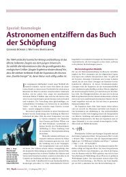
Figure 6.1. Example of the solution of a linear Riemann problem with constant and diagonal
advection matrix. Top: initial condition (solid line is q 1 , dashed line is q 2 ). Bottom: after some
time, the q 1 component has moved to the right (λ 1 > 0) while the q 2 component has moved to
the left (λ 2 < 0).
For hydrodynamic problems such shock tube tests are used to test the performance of numerical
hydrodynamics algorithms. This was first done by (Sod 1978, J. Comp. Phys 27, 1),
hence the name Sod shock tube tests. But such tests were also carried out in the laboratory (see
e.g. the book by Liepmann & Roshko).
6.2.1 Riemann problems for linear advection problems
The simplest Riemann problems are those of linear advection problems with constant advection
velocity, or constant Jacobian matrix. Consider the following equation:
∂ t
(
q1
q 2
)
+
Consider the following Riemann problem for this set of equations:
( ) ( )
λ1 0 q1
∂
0 λ x =0 (6.9)
2 q 2
q 1 (x, 0) =
q 2 (x, 0) =
{
q1,l for x0
{
q2,l for x0
(6.10)
(6.11)
Clearly the solution is:
q 1 (x, t) = q 1 (x − λ 1 t, 0) (6.12)
q 2 (x, t) = q 2 (x − λ 2 t, 0) (6.13)
which is simply that the function q 1 (x) is shifted with velocity λ 1 and the function q 2 (x) is shifted
with velocity λ 2 . An example is shown in Fig. 6.1 A very similar solution is found if the matrix
is not diagonal, but has real eigenvalues: we then simply decompose (q 1 ,q 2 ) into eigenvectors,
obtaining (˜q 1 , ˜q 2 ), shift ˜q 1 and ˜q 2 according to their own advection velocity (eigenvalue of the
matrix), and then reconstruct the q 1 and q 2 from ˜q 1 and ˜q 2 .

99
t
x
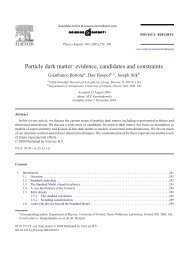
Figure 6.2. The characteristics of the problem solved in Fig. 6.1.
→ Exercise: Solve in this way the general Riemann problem for the equation
( ) ( ) ( )
q1 0 1 q1
∂ t + ∂
q 2 1 0 x =0 (6.14)
q 2
These examples are for hyperbolic equations with two characteristics, but this procedure
can be done for any number of characteristics.
Note that if we look at this problem in an (x, t) diagram, then we see two waves propagating,
one moving with velocity λ 1 and one with velocity λ 2 . We also see that the solution is selfsimilar:
q 1,2 (x, t b )=q 1,2 (xt a /t b ,t a ) (6.15)
6.3 Riemann problems for the equations of hydrodynamics
Riemann problems for the Euler equations are much more complex than those for the simple
linear hyperbolic equations shown above. This is because of the strong non-linearity of the
equations. A Riemann problem for the equations of hydrodynamics is defined as:
ρ, u, P =
{
ρl ,u l ,P l for x0
(6.16)
The general solution is quite complex and even the qualitative shape of the solution depends
strongly on the Riemann problem at hand. In this section we will discuss two special cases.
6.3.1 Special case: The converging flow test
The simplest Riemann problem for the hydrodynamic equation is that in which P l = P r , ρ l = ρ r
and u l = −u r with u l > 0. This is a symmetric case in which the gas on both sides of the
dividing line are moving toward each other: a converging flow. From intuition and/or from
numerical experience it can be said that the resulting solution is a compressed region that is
expanding in the form of two shock waves moving away from each other. Without a-priori proof
(we shall check a-posteriori) let us assume that the compressed region in between the two shock
waves has a constant density and pressure, and by symmetry has a zero velocity. We also assume
that the converging gas that has not yet gone through the shock front is undisturbed.
The problem we now have to solve is to find the shock velocity v s (which is the same but
opposite in each direction) and the density and pressure in the compressed region: ρ c , P c . For a

100
given v s the Mach number M of the shock is:
M = u l + v s
C s,l
=(u l + v s )
√
P l
γρ l
(6.17)
(we take by definition v s > 0). We now need the Rankine-Hugoniot adiabat in the form of
Eq. (1.97),
ρ 1
= (γ − 1)M2 +2
= γ − 1
ρ c (γ + 1)M 2 γ +1 + 2
(6.18)
(γ + 1)M 2
as well as the condition for mass conservation
ρ l (u l + v s )=ρ c v s (6.19)
By writing v s = v s + u l − u l =(M− u l /C s,l )C s,l in the latter equation we can eliminate ρ l /ρ c
in both equations to obtain
which reduces to
The solution is:
M = 1 2
γ − 1
γ +1 M2 + 2
γ +1 = M2 − u l
M (6.20)
C s,l
M 2 − γ +1
2
{ (γ +1
2
u l
C s,l
M− 1 = 0 (6.21)
) √
ul (γ + 1)
±
2
C s,l 4
u 2 l
C 2 s,l
+4
}
(6.22)
For our purpose we need to choose the positive root. One sees that there is always a solution,
and that one can find two limits:
• Limit 1, u l ≪ C s,l : The solution is M =1. This means that in this limit the shock wave
reduces to a sound wave.
• Limit 2, u l ≫ C s,l : The solution is M =(u l /C s,l )(γ + 1)/2. This is the strong shock limit:
the compression reaches its maximum of ρ c → ρ l (γ + 1)/(γ − 1). The strong shock limit
is the limit in which the pre-shock thermal energy is so small compared to the post-shock
value that it can be regarded as being zero.
6.3.2 Special case: Sod’s shock tube tests
A special case of a Riemann problem in Eulerian hydrodynamics is when the initial state has
zero velocity on both sides of the dividing point, but the pressure has a jump. We shall discuss
these solutions here following the book by Bodenheimer et al. (2007). The complete solution of
the Sod shock tube test is rather difficult to derive, so here we shall derive only the most obvious
relations, and write down other relations without derivation.
The most important first step is to find out what the qualitative form of the solution is. Here
we rely on experience: If one solves such problems using numerical hydrodynamics or laboratory
experiments one finds that the self-similar solution that follows from such a problem typically
has 5 regions which we shall call region 1,2,3,4,5 as depicted in Fig. 6.3. Region 1 and 5 have
states which correspond to the left and the right initial state respectively. Regions 3 and 4 have
steady states (independent of x within the region) and region 2 has an x-dependent state. This

101
1 2 3 4
5
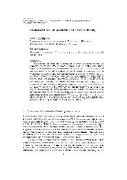
Figure 6.3. The solution to the shock tube problem of Sod for γ =7/5, ρ l = 10 5 , P l =1,
ρ r =1.25 × 10 4 and P r =0.1, shown at time t = 5000. The regions 1 to 5, as mentioned in
the text, are annotated at the top.
region 2 represents an expansion wave, also called rarefaction wave. This is a simple wave of the
left-going characteristic family (the 1-characteristic family in the terminology of Section 6.1). It
is the only non-constant region in the solution. The dividing line between region 3 and 4 is a
contact discontinuity, i.e. a line separating two fluids of different entropy but the same pressure
and the same velocity. This is a “wave” of the middle characteristic family (the 2-characteristic
family in the terminology of Section 6.1). Therefore u 3 = u 4 and P 3 = P 4 . The propagation
speed of the contact discontinuity is therefore also u c = u 4 and the location of this discontinuity
at some time t is x contact = u c t. Regions 4 and 5 are separated by a forward moving shock wave.
This is a jump in the forward moving characteristic family (the 3-characteristic family in the
terminology of Section 6.1). Since u 5 =0one can invoke mass conservation to write the shock
propagation speed u s in terms of the velocity u 4 and the densities in both regions:
u s = u 4
ρ 4
ρ 4 − ρ 5
(6.23)
The location of the shock wave at time t is therefore x shock = u s t. According to the Rankine-
Hugoniot conditions derived in Section 1.9 we can also relate the density ratio and the pressure
ratio over the shock:
ρ 4
= P 4 + m 2 P 5
(6.24)
ρ 5 P 5 + m 2 P 4
where m 2 =(γ−1)/(γ+1). From these relations we can derive the velocity in region 4, because
we know that u 5 =0. We obtain
√
1 − m
u 4 =(P 4 − P 5 )
2
ρ 5 (P 4 + m 2 P 5 )
(6.25)

102
This is about as far as we get on the shock front. Let us now focus on the expansion wave (region
2). The leftmost onset of the expansion wave propagates to the left with the local sound speed.
So we have, at some time t, this point located at x wave = −C s,1 t, where C s,1 = √ γP 1 /ρ 1 is the
sound speed in region 1. Without further derivation (see Hawley et al. 1984) we write that the
gas velocity in region 2 can be expressed as
u 2 =
√
(1 − m 4 )P 1/γ (
1
P
m 4 ρ 1
γ−1
2γ
1 − P
γ−1
2γ
2
)
(6.26)
To find the dividing line between regions 2 and 3 we now solve the equation u 2 = u 4 , i.e. Eq.(6.26)
− Eq.(6.25)= 0, for the only remaining unknown P 3 . We do this using a numerical root-finding
method, for instance the zbrent method of the book Numerical Recipes by Press et al.. This
will yield us a numerical value for P 3 = P 4 . Then Eq.(6.25) directly leads to u c = u 3 = u 4 .
The Hugoniot adiabat of the shock (Eq. 6.24) now gives us ρ 4 . Now with Eq. (6.23) we can
compute the shock velocity u s , and thereby the location of the shock front x shock = u s t. The
density in region 3 can be found by realizing that none of the gas to the left of the contact discontinuity
has ever gone through a shock front. It must therefore still have the same entropy as
the gas in region 1. Using the law for polytropic gases P = Kρ γ we can say that K is the same
everywhere left of the contact discontinuity (i.e. in regions 1,2 and 3). Therefore we can write
that ρ 3 = ρ 1 (P 3 /P 1 ) 1/γ . At this point we know the density, the pressure and the gas velocity
in regions 1,3,4,5. We can therefore easily calculate any of the other quantities in these regions,
such as the sound speed C s or the internal thermal energy e th . The remaining unknown region
is region 2, and we also do not yet know the location of the separation between regions 2 and 3.
Without derivation (see Hawley et al. 1984) we state that in region 2:
u(x, t) = (1 − m 2 )
( x
t + C s,1
)
(6.27)
which indeed has the property that u = 0 at x = −C s,1 t. We can find the location of the
separation between regions 2 and 3 by numerically solving u(x, t) =u 3 for x. The expression for
the sound speed C s (x, t) in region 2 is now derived by noting that region 2 is a classical expansion
fan, in which the left-moving characteristic λ − must, by nature of self-similar solutions, have the
form λ − ≡ u(x, t) − C s (x, t) =x/t. This yields for region 2:
Cs 2 P (x, t)
(x, t) ≡ γ
(u(x,
ρ(x, t) = t) − x ) 2
(6.28)
t
Also here we know that P (x, t) =Kρ(x, t) γ with the same K as in region 1. Therefore we
obtain:
[ ρ
γ
1
ρ(x, t) =
(u(x, t) − x ) ] 2 1/(γ−1)
(6.29)
γP 1 t
from which P (x, t) can be directly derived using P (x, t) =Kρ(x, t) γ , and the sound speed and
internal thermal energy follow then immediately. We now have the total solution complete, and
for a particular example this solution is shown in Fig. 6.3. Later in this chapter we shall use
these solutions as simple test cases to verify the accuracy and performance of hydrodynamic
algorithms.

103
t
x
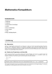
Figure 6.4. Godunov’s method: solving a self-similar Riemann problem at each interface
(grey), and making sure that the time step is small enough that they do not overlap. The two
leftmost self-similar Riemann solutions just manage to touch by the end of the time step, which
means that the time step can not be made larger before they will interfere.
6.4 Godunov’s method
We can now apply what we learned about the solution of Riemann problems to devise a new
numerical method for numerical hydrodynamics. Consider our numerical solution at some time
t n to be given by q n i . These are values of q given at the cell centers located at x = x i. We define
cell interfaces x i+1/2 in the usual way (see Chapter 4) to be located in between the cell centers x i
and x i+1 . As our subgrid model we assume that at the start of the time step the state within each
cell is strictly constant (piecewise constant method, see Chapter 4). At each interface the state
variables now describe a jump. If we zoom in to the region around this interface we see that this
is precisely the definition of a Riemann problem, but this time locally within the two adjacent
cells. We can now calculate what the self-similar solution of the Riemann problem at each cell
interface i +1/2 would be. This is a subgrid analytic evolution of the hydrodynamic system
within each pair of cells. This self-similar solution is calculated at each interface, so in order
to preserve the self-similar character of these solutions we must prevent the solutions from two
adjacent interfaces to overlap. This is depicted in Fig. 6.4. The time step is therefore restricted
to
∆t ≤ min(∆t i ) (6.30)
where
∆t i =
x i+1/2 − x i−1/2
max(λ i−1/2,k+ ) − min(λ i+1/2,k− )
(6.31)
where λ i−1/2,k+ denotes the maximum positive eigenvalue at interface i − 1/2, and will be 0 in
case no positive eigenvalues exist at that interface. Likewise λ i+1/2,k− denotes the smallest (i.e.
most negative) negative eigenvalue at interface i +1/2, or 0 if no negative eigenvalues exist.
How to proceed from here, i.e. how to create a numerical algorithm from this concept, can
be seen in two different way, which we will highlight in the two next subsections.
6.4.1 One way to look at Godunov’s method
At the end of the time step each cell i consists of three regions: a left region which is affected
by the Riemann solution at interface i − 1/2, a middle region which is not yet affected, and a
right region which is affected by the Riemann solution at interface i +1/2. Since we know the
(semi-)analytic solutions of the Riemann problems and we of course know the unaffected state
in the middle region, we can (semi-)analytically average all state variables over the cell. This
averaging then results in the cell-center value of q n+1
i . This averaging procedure is very similar to
what was done in the donor-cell algorithm, but this time the state in the cell at the end of the time
step is far more complex than in the simple donor-cell algorithm. Because of this complexity we
shall not work this out in this chapter.

104
6.4.2 Another way to look at Godunov’s method
Another way to look at Godunov’s method is by looking at the flux at the interface. We know
that the Riemann solutions around the cell interfaces are self-similar in the dimensionless space
variable ξ =(x − x i+1/2 )/(t − t n ). This means that the state at the interface in this solution is
constant in time (at least between t = t n and t = t n+1 ). This then implies that the flux f i+1/2 is
also constant in this time interval. We can therefore then write:
q n+1
i
= q n i − ∆t f n i+1/2 − f n i−1/2
x i+1/2 − x i−1/2
(6.32)
where fi+1/2 n and f i−1/2 n are the fluxes calculated from the Riemann problems at the cell interfaces.
Note that this is true as much for linear sets of hyperbolic equations as well as for
non-linear ones. The complexity still remains in determining the state in the Riemann problem
at the cell interfaces, but that is already much less difficult than determining the entire Riemann
solution and averaging over it. Nevertheless for hydrodynamics the method remains complex
and we will therefore not go into the Godunov method for these equations.
6.5 Godunov for linear hyperbolic problems: a characteristic solver
6.5.1 Example for two coupled equations
Instead of demonstrating how a Godunov solver works for the full non-linear set of equations
of hydrodynamics, we show here how it works for linear hyperbolic sets of equations. The nice
thing is that in this case the Riemann problem at each cell interface can be solved analytically.
Moreover, we will then naturally be led to a new concept: that of a characteristic solver. For
linear problems Riemann solvers and characteristic solvers are identical. Later, when dealing
with the full set of non-linear hydrodynamics equations, we shall be using both concepts.
Let us consider the following equation:
( ) ( )
q1 a b
∂ t +
q 2 c d
∂ x
(
q1
q 2
)
=0 (6.33)
where the matrix is diagonizable and has two real eigenvalues. We wish to solve this numerically.
Since the advection matrix, in this example, is constant, we were able to bring it out of the ∂ x
operator without flux conservation violation. The way we proceed is first to define the state
vector on the left- and right- side of the interface i +1/2:
q i+1/2,L ≡ q i (6.34)
q i+1/2,R ≡ q i+1 (6.35)
Now define the eigenvalues and eigenvectors of the problem:
λ (±) = 1 {
(a + d) ± √ }
(a − d)
2
2 +4bc
(6.36)
and
( )
λ(±) +2d
e (±) =
2c
(6.37)
Note that we use indices (−) and (+) because in this special case the eigenvalues are clearly
identifiable with left- and right-moving characteristics unless the problem is “supersonic” in that

105
both eigenvalues are negative or both are positive. In general we would simply use λ 1 , λ 2 etc.
This is just a notation issue. Now, any state
( )
q1
q =
(6.38)
q 2
can be decomposed into these eigenvectors:
˜q (−) =
˜q (+) =
{ }
1 λ(+) +2d
q 2 − q 1
λ (+) − λ (−) 2c
{ }
1 λ(−) +2d
q 2 − q 1
λ (−) − λ (+) 2c
So we can define the decomposed state on each side of the interface:
(6.39)
(6.40)
˜q (−),i+1/2,L = ˜q (−),i (6.41)
˜q (+),i+1/2,L = ˜q (+),i (6.42)
˜q (−),i+1/2,R = ˜q (−),i+1 (6.43)
˜q (+),i+1/2,R = ˜q (+),i+1 (6.44)
Now we can construct the flux at the interface. Suppose that λ 1 > 0, then clearly the flux for
˜q (+),i+1/2 is determined solely by ˜q (+),i+1/2,L and not by ˜q (+),i+1/2,R (the upwind principle):
˜f (−),i+1/2 =
{
λ(−)˜q (−),i+1/2,L for λ (−) > 0
λ (−)˜q (−),i+1/2,R for λ (−) < 0
and similar for ˜f (+),i+1/2 . The total flux for q is then:
(6.45)
f i+1/2 = ˜f (−),i+1/2 e (−) + ˜f (+),i+1/2 e (+) (6.46)
We see that Godunov’s method for linear advection equations is nothing else than the donor-cell
algorithm applied to each characteristic separately.
We can generalize this method to non-constant advection matrix. Consider the following
problem:
∂ t
(
q1
q 2
)
[( )( )]
a(x) b(x)
+ ∂
q1
x =0 (6.47)
c(x) d(x) q 2
The procedure is now the same, except that we must do the eigenvector decomposition with the
local matrix at the interface i +1/2. Both the eigenvectors and the eigenvalues are now local to
the interface, and so will the decomposition be. In this case ˜q (−),i+1/2,L ≠˜q (−),i−1/2,R , while in
the case of constant matrix we had ˜q (−),i+1/2,L =˜q (−),i−1/2,R . For the rest we construct the fluxes
in the same way as above for the constant matrix.
We see that in the simple case of linear advection problems, the Godunov method (based
on the Riemann problem) is actually nothing else than a characteristic solver: the problem is
decomposed into characteristics, which are advected each in their own directions. Indeed, for
linear problems the principle of using Riemann problems at each interface to perform the numerical
integration of the equations is identical to the principle of decomposing into the eigenvectors
of the Jacobian and advecting each component with its own eigenvalue as characteristic speed.
In other words: For linear problems a Riemann solver is identical to a characteristic solver. This
is not true anymore for non-linear problems: as we shall see later on, a characteristic solver for
hydrodynamics is not a true Riemann solver but an approximate Riemann solver or equivalently
a linearized Riemann solver. However, let us, for now, stick to linear problems a bit longer.

106
6.5.2 General expressions for Godunov solvers for linear problems
We can make a general expression for the flux, for any number of characteristics:
f i+1/2 =
∑ ˜f k,i+1/2 e k (6.48)
k=1···K
where K is the number of characteristics (i.e. number coupled equations, or number of eigenvectors
and eigenvalues), and where
˜f k,i+1/2 = 1 [
]
2 λ k (1 + θ k )˜q i n + (1 − θ k )˜q i+1
n (6.49)
where θ k =1if λ k > 0 and θ k = −1 if λ k < 0. This is identical to the expressions we derived
in Subsection 6.5, but now more general.
6.5.3 Higher order Godunov scheme
As we know from Chapter 4, the donor-cell algorithm is not the most sophisticated advection
algorithm. We therefore expect the solutions based on Eq. (6.49) to be smeared out quite a bit.
In Chapter 4 we found solutions to this problem by dropping the condition that the states are
piecewise constant (as we have done in the Godunov scheme so far) and introduce a piecewise
linear subgrid model, possibly with a flux limiter. In principle, for linear problems the Godunov
scheme is identical to the advection problem for each individual characteristic, and therefore we
can apply such linear subgrid models here too. In this way we generalize the Godunov scheme in
such a way that we have a slightly more complex subgrid model in each cell (i.e. non-constant),
but the principle remains the same. At each interface we define ˜r k,i−1/2 :
⎧
⎪⎨
˜r k,i−1/2 n =
⎪⎩
˜q n k,i−1 −˜qn k,i−2
˜q n k,i −˜qn k,i−1
˜q n k,i+1 −˜qn k,i
˜q n k,i −˜qn k,i−1
for λ k,i−1/2 ≥ 0
for λ k,i−1/2 ≤ 0
(6.50)
where again k denotes the eigenvector/-value, i.e. the characteristic. We can now define the flux
limiter ˜φ(˜r k,i−1/2 ) for each of these characteristics according to the formulae in Section 4.5 (i.e.
Eqs. 4.39, 4.40, 4.41). Then the flux is given by (cf. Eq. 4.38)
˜f n+1/2
k,i−1/2 =1 2 λ k,i−1/2
1
2 |λ k,i−1/2|
[
]
(1 + θ k,i−1/2 )˜q k,i−1/2,L n + (1 − θ k,i−1/2)˜q k,i−1/2,R
n +
(
) 1 −
λ k,i−1/2 ∆t
(6.51)
∣ ∆x ∣ φ(˜r k,i−1/2 n )(˜qn k,i−1/2,R − ˜qn k,i−1/2,L )
It is useful, for later, to derive an alternative form of this same equation, which can be obtain
with a bit of algebraic manipulation starting from Eq. (6.51). We use the identity |λ k,i−1/2 | =
θ k,i−1/2 λ k,i−1/2 and the definition ɛ k,i−1/2 ≡ λ k,i−1/2 ∆t/(x i − x i−1 ) and obtain:
˜f n+1/2
k,i−1/2 = 1 2 λ k,i−1/2(˜q n k,i−1/2,R +˜qn k,i−1/2,L )
− 1 2 λ k,i−1/2(˜q n k,i−1/2,R − ˜qn k,i−1/2,L )[θ k,i−1/2 + ˜φ k,i−1/2 (ɛ k,i−1/2 − θ k,i−1/2 )]
(6.52)
where ˜φ k,i−1/2 ≡ φ(˜r k,i−1/2 ). If we define the decomposed fluxes at the left and right side of the
interface as
˜f k,i−1/2,L = λ i−1/2˜q k,i−1/2,L (6.53)
˜f k,i−1/2,R = λ i−1/2˜q k,i−1/2,R (6.54)

107
then we obtain:
˜f n+1/2
k,i−1/2 = 1 2 ( ˜f n k,i−1/2,R + ˜f n k,i−1/2,L )
− 1 2 ( ˜f n k,i−1/2,R − ˜f n k,i−1/2,L)[θ k,i−1/2 + ˜φ k,i−1/2 (ɛ k,i−1/2 − θ k,i−1/2 )]
(6.55)
Now we can arrive at our final expression by adding up all the partial fluxes (i.e. the fluxes of all
eigen-components):
f n+1/2
i−1/2
= 1(f n 2 i−1/2,R + fi−1/2,L)
n
∑
( ˜f k,i−1/2,R n − ˜f k,i−1/2,L)[θ n k,i−1/2 + ˜φ k,i−1/2 (ɛ k,i−1/2 − θ k,i−1/2 )]
− 1 2
k=1···K
(6.56)
This is our final expression for the (time-step-averaged) interface flux.
There are a number of things we can learn from this expression:
1. The interface flux is the simple average flux plus a diffusive correction term. All the
ingenuity of the characteristic solver lies in the diffusive correction term.
2. The flux limiter can be seen as a switch between donor-cell (˜φ =0) and Lax-Wendroff
( ˜φ =1), where we here see yet again another interpretation of Lax-Wendroff: the method
in which the interface flux is found using a linear upwind interpolation (in contrast to
upwinding, where the new state is found using linear upwind interpolation). Of course, if
˜φ is one of the other expressions from Section 4.5, we get the various other schemes.
In all these derivations we must keep in mind the following caveats:
• Now that the states in the adjacent cells is no longer constant, the Riemann problem is no
longer self-similar: The flux at the interface changes with time.
• In case the advection matrix is non-constant in space, the determination of the slopes becomes
a bit less mathematically clean: Since the eigenvectors now change from one cell
interface to the next, the meaning of ˜q k,i+1/2,R − ˜q k,i+1/2,L is no longer identical to the meaning
of ˜q k,i−1/2,R − ˜q k,i−1/2,L . Although the method works well, the mathematical foundation
for this method is now slightly less strong.
6.6 The MUSCL-Hancock scheme
So far we have constructed a general recipe for Riemann solvers / Godunov schemes. Higher
order Riemann solvers were created using flux limiters in Subsection 6.5.3.
Many codes, however, use a different method for making higher order Riemann solvers.
Their philosophy goes back to the idea of slope limiters instead of flux limiters. In other words:
they use a linear subgrid model. Some codes go even further and use a parabolic subgrid model
(the PPM method). The philosophy of how to make Riemann solvers higher order is very different
from how it is done in Subsection 6.5.3. In this Section we will discuss the MUSCL-Hancock
scheme which uses slope limiters as linear subgrid models.
Let us again consider a set of quantities q k,i with k =1,K, as before. Now let us apply the
usual slope limiter techniques to each quantity q k separately, thereby completely ignoring any
of our knowledge of the characteristic eigenvectors of the system. We simply treat each q k as if

108
it is an independent scalar, and thus we acquire linear subgrid models in each cell i for each q k :
q k (x, t) i . These subgrid models allow us to define left- and right- interface values for q k :
q n k,i−1/2,L = qn k,i−1 + 1 2 ∆xσ k,i−1 (6.57)
q n k,i−1/2,R = q n k,i − 1 2 ∆xσ k,i (6.58)
q n k,i+1/2,L = qn k,i + 1 2 ∆xσ k,i (6.59)
q n k,i+1/2,R = q n k,i+1 − 1 2 ∆xσ k,i+1 (6.60)
These values now define Riemann problems at the interfaces and we can use our knowledge of
the solutions to these Riemann problems to compute the interface flux. There are, however, two
major caveats:
1. We will see below that at this point we will need to advance these values half a timestep
into the future before we use them in the Riemann problem.
2. Strictly speaking the Riemann problems defined here are not like the classical Riemann
problem in which the states on both sides are constant in space. In this case the quantities
in principle have a linear dependence on x away from the boundary. However, in the
MUSCL-Hancock scheme this is ignored: the Riemann problem to be solved is as if the
state is constant on each side, with the values given by the linear extrapolation (advanced
half a time step in the future). The error made here is, to linear order, compensated by the
half-time-step advance.
It is an interesting exercise to see what happens if we do not advance the qk,i±1/2,L/R n half a time
step into the future: the scheme will be unstable. So how do we do this half time step update of
qk,i±1/2,L/R n ? In the MUSCL-Hancock scheme it is done in the following way:
k,i−1/2,L = qn k,i−1/2,L + 1 ∆t
2 ∆x (f k[qi−1/2,L] n − f k [q i−3/2,R ]) (6.61)
k,i−1/2,R = qn k,i−1/2,R + 1 ∆t
2 ∆x (f k[qi+1/2,L] n − f k [q i−1/2,R ]) (6.62)
k,i+1/2,L = qn k,i+1/2,L + 1 ∆t
2 ∆x (f k[qi+1/2,L] n − f k [q i−1/2,R ]) (6.63)
k,i+1/2,R = qn k,i+1/2,R + 1 ∆t
2 ∆x (f k[qi+3/2,L] n − f k [q i+1/2,R ]) (6.64)
q n+1/2
q n+1/2
q n+1/2
q n+1/2
where f k [q] is the k-component of the flux constructed from q =(q 1 , ··· ,q K ).
If we now insert the q n+1/2
n+1/2
k,i±1/2,L/R
into our Riemann problem solver, then the flux fk,i±1/2 that
comes out of this solver is the flux we use to update our q k,i values:
q n+1
k,i
= qk,i n + ∆t n+1/2
(fk,i−1/2 ∆x − f n+1/2
k,i+1/2 ) (6.65)
This method is stable, and it is so general, that it can be easily applied to very non-linear problems.
→ Exercise: Apply this method to a simple scalar advection equation with u =1, and with
unspecified (i.e. arbitrary) slope limiter (i.e. use the σ slope symbol without substituting a
specific slope limiter) and show that the MUSCL-Hancock scheme for this simple system
actually reduces to the standard advection method with piecewise linear subgrid model (Eq.
4.21 of Chapter 4).