Angewandte Regelung und Optimierung in der ... - uni-stuttgart
Angewandte Regelung und Optimierung in der ... - uni-stuttgart
Angewandte Regelung und Optimierung in der ... - uni-stuttgart

Create successful ePaper yourself
Turn your PDF publications into a flip-book with our unique Google optimized e-Paper software.
Alexan<strong>der</strong> Horch<br />
<strong>Angewandte</strong> <strong>Regelung</strong> <strong>und</strong> <strong>Optimierung</strong><br />
<strong>in</strong> <strong>der</strong> Prozess<strong>in</strong>dustrie<br />
9. <strong>Optimierung</strong> von Wassernetzen<br />
© A.Horch<br />
SS 2010 | Slide 1
Inhalt<br />
• Überblick über die Wasserwirtschaft<br />
• Automatisierungsbedarfe<br />
• Beispiele ausgeführter <strong>Regelung</strong> & <strong>Optimierung</strong><br />
• Leckageerkennung / Entscheidungsunterstützung<br />
• Pumpen- <strong>und</strong> Ventile<strong>in</strong>satzplanung<br />
• Zusammenfassung<br />
© ABB Group<br />
SS 2010 | Slide 2
Wasserversorgung - Globale Sicht<br />
Klimawandel<br />
Auswirkungen des Klimawandels werden stärker wahrnehmbar → verän<strong>der</strong>tes<br />
Bewusstse<strong>in</strong><br />
Klimawandel bee<strong>in</strong>flusst Wasserversorgungssituation <strong>in</strong> vielen Regionen<br />
Ineffizienzen <strong>in</strong> <strong>der</strong> Wasserversorgung → negativer Beitrag<br />
Randnotiz: ~20% <strong>der</strong> globalen elektrischen Energie werden zum Betrieb von<br />
Pumpen <strong>und</strong> Pumpsystemen verwendet* → Wasserversorgung ist e<strong>in</strong>es <strong>der</strong><br />
Hauptanwendungsfel<strong>der</strong><br />
Herausfor<strong>der</strong>ung: Erhöhung <strong>der</strong> Energieeffizienz zur Reduktion <strong>der</strong><br />
Treibhausgasemissionen<br />
Source: Factiva, UK<br />
English language press<br />
mentions <strong>in</strong>clud<strong>in</strong>g global<br />
warm<strong>in</strong>g,<br />
climate change,<br />
greenhouse effect or<br />
greenhouse gas<br />
Taken from presentation<br />
“Local Authority Carbon<br />
Management Program”,<br />
Richard Rugg,<br />
Derby City Council, 2007<br />
© ABB Group<br />
June 28, 2010 | Slide 3<br />
•*Source: Protect<strong>in</strong>g the environment and reduc<strong>in</strong>g costs, Sulzer AG, Sulzer Technical Review, 1/2009
Wasserversorgung - Globale Sicht<br />
Wasserknappheit<br />
Wasserknappheit ist e<strong>in</strong> Problem <strong>in</strong> vielen Regionen <strong>der</strong> Welt<br />
Globaler Wasserverbrauch wird Schätzungen nach um 40% bis 2025 steigen<br />
Ineffizienzen <strong>in</strong> Wassertransport <strong>und</strong> –verteilung tragen zusätzlich zur<br />
Verschlechterung <strong>der</strong> Versorgungssituation bei<br />
Leckageverluste bei teilweise über 50% <strong>der</strong> Versorgungsmenge<br />
~90% Untergr<strong>und</strong>verluste, ~10% grosse Rohrbrüche<br />
Herausfor<strong>der</strong>ung: Reduzierung <strong>der</strong> Verluste bei Transport <strong>und</strong> Verteilung → ger<strong>in</strong>gere<br />
energetische Aufwendungen zum Ausgleich <strong>der</strong> Verluste<br />
Wasserknappheit<br />
Zunehmende<br />
Verknappung<br />
Ausreichende<br />
Wasserressourcen<br />
Wasserüberschuss<br />
Source: Waterworks<br />
Sonneberg<br />
© ABB Group<br />
June 28, 2010 | Slide 4
Wasserverwendung weltweit<br />
Schlüsselressource<br />
© ABB Group<br />
June 28, 2010 | Slide 5
Water<br />
Automation Applications<br />
• Pump<strong>in</strong>g Stations<br />
• Efficient pump<strong>in</strong>g station design improves plant availability and output, thereby reduc<strong>in</strong>g the<br />
costs of water supply and treatment.<br />
• M<strong>uni</strong>cipal Wastewater Treatment and Recycl<strong>in</strong>g<br />
• Treatment must guarantee water quality before (re-)use and m<strong>in</strong>imise the impact on the<br />
environment<br />
• Water Distribution<br />
• Network management solutions for real-time monitor<strong>in</strong>g and control of distributed water<br />
systems<br />
• Industrial Water Treatment and Recycl<strong>in</strong>g<br />
• Basic onsite treatment of waste process water avoids unnecessary use of potable water and<br />
costly discharges to public wastewater collection. Industry uses ~20% of available water.<br />
• Desal<strong>in</strong>ation Plants<br />
• Desal<strong>in</strong>ation plays an essential role where demand for potable water outpaces the<br />
availability of natural resources<br />
• Water Transmission<br />
• Infrastructures to transport over long distances to reduce mismatch between supply and<br />
demand<br />
• Irrigation<br />
• 80% of potable water is used for irrigation<br />
© ABB Group<br />
SS 2010 | Slide 6
Randnotiz<br />
Beispiel - Verluste <strong>in</strong> europäischen Tr<strong>in</strong>kwassernetzen<br />
© ABB Group<br />
June 28, 2010 | Slide 7
Wasserversorgung - Globale Sicht<br />
Potentiale<br />
Schwerpunkt liegt auf Wassertransport <strong>und</strong> –verteilnetzen<br />
Reduzierung von Verlusten durch Leckagen<br />
Erhebliche Potentiale für Erhöhung <strong>der</strong> Energieeffizienz<br />
Lösungsansatz → umfassendes Wassermanagement<br />
E<strong>in</strong>satz neuster Technologien → von <strong>der</strong> Feldebene bis h<strong>in</strong> zu<br />
höherwertigen Anwendungen (Simulation, <strong>Optimierung</strong>)<br />
Druckmanagement, Ressourcenmanagement,<br />
Energiemanagement,…<br />
E<strong>in</strong>b<strong>in</strong>dung <strong>in</strong> e<strong>in</strong>e <strong>in</strong>tegrierte Systemumgebung ermöglicht<br />
Generierung e<strong>in</strong>es hohen Nutzwerts (Daten<strong>in</strong>tegration,<br />
Oberflächen<strong>in</strong>tegration)<br />
© ABB Group<br />
June 28, 2010 | Slide 8<br />
‣ Nutzung vorhandener <strong>und</strong> Generierung zusätzlicher Daten <strong>und</strong><br />
Informationen zur <strong>Optimierung</strong> des Wassernetzbetriebs<br />
‣ Schwerpunkt des Vortrags auf <strong>in</strong>tegriertem Ansatz zum<br />
Wassermanagement
Wichtige Marktreiber<br />
Worauf sich Wasserversorger fokussieren…<br />
Erhöhung <strong>der</strong> Energieeffizienz<br />
Begrenzung steigen<strong>der</strong> Energiekosten<br />
Nachhaltigkeitsaspekte<br />
Reduktion von Leckagen („Non-Revenue Water“)<br />
Verbesserte Leckageerkennung <strong>und</strong> – lokation<br />
Verkürzte Reaktionszeit für<br />
Reparaturmaßnahmen<br />
Kostenreduktion<br />
Reduktion von Betrieb- <strong>und</strong><br />
Instandhaltungskosten sowie Investitionskosten<br />
Stärkere Orientierung auf f<strong>in</strong>anziell<br />
herausragende Ergebnisse<br />
Verbesserung <strong>der</strong> Versorgungsqualität <strong>und</strong> -<br />
sicherheit<br />
M<strong>in</strong>imierung <strong>der</strong> Anzahl an Unterbrechungen,<br />
stabil hohe Wasserqualität,…<br />
Grosse<br />
Rohrbrüche<br />
Untergr<strong>und</strong>verluste<br />
© ABB Group<br />
June 28, 2010 | Slide 9
Introduction –<br />
Side Note<br />
Randnotiz<br />
Strategie zur Leckagereduktion<br />
Strategische<br />
Herangehensweise zur<br />
Reduzierung <strong>der</strong><br />
Leckagen/Leckageflüssen<br />
notwendig<br />
Druckmanagement ist<br />
elementar → bee<strong>in</strong>flusst<br />
Energieverbrauch <strong>und</strong><br />
Auftreten neuer Leckagen<br />
sowie Flüsse aus<br />
exisitierenden Leckagen<br />
© ABB Group<br />
June 28, 2010 | Slide 10
Wasser<br />
Aktueller Megatrend mit Folgen<br />
• ZVEI Roadmap Automation 2020+: Wasser <strong>und</strong> Abwasser<br />
• Megatrends (Bevölkerungswachstum, Urbanisierung,<br />
Klimawandel, ...) werden den Druck, Wasser effizienter zu nutzen,<br />
neue Wasserquellen zu erschließen <strong>und</strong> die Abwasserent-sorgung<br />
zu verbessern, verstärken.<br />
• Zunehmen<strong>der</strong> Kostendruck<br />
• Paradigmenwechsel vom „Schadstoffentsorgungssystem“ zur<br />
Nutzung von Abwasser als Wertstoff ab.<br />
• Der Markt für Meerwasserentsalzung <strong>und</strong> Aufarbeitung von<br />
gebrauchtem Wasser wird sich stark vergrößern (2-3 fach).<br />
• Umfangreiche Mess-, Steuer- <strong>und</strong> <strong>Regelung</strong>stechnik werden<br />
<strong>in</strong>sbeson<strong>der</strong>e für <strong>in</strong>tegrierte Wassermanagementansätze benötigt.<br />
• Steigende Nachfrage nach Kle<strong>in</strong>kläranlagen.<br />
• Sicherheit von Wassernetzen (Verschmutzung, Terror).<br />
• Von Messgeräten <strong>und</strong> Sensoren wird erwartet, dass sie robust,<br />
günstig <strong>und</strong> wartungsarm s<strong>in</strong>d.<br />
© ABB Group<br />
SS 2010 | Slide 11
Wasser<br />
Aktueller Megatrend – auch für Automatisierung<br />
Investitionen <strong>in</strong><br />
• Meerwasserentsalzung<br />
• Tr<strong>in</strong>kwassergew<strong>in</strong>nung aus Abwasser<br />
• Erkennung von Arzneimittelrückständen <strong>und</strong><br />
an<strong>der</strong>en Spurenstoffen <strong>in</strong> Abwässern<br />
• Risikomanagement: Schutz kritischer<br />
Wasser<strong>in</strong>frastrukturen<br />
• Kanalnetzbewirtschaftung<br />
• Energetische Klärschlammnutzung<br />
• Rückgew<strong>in</strong>nung von Phosphor aus<br />
Klärschlamm<br />
Schlüsseltechnologien <strong>der</strong><br />
Automatisierung<br />
• Sensorik <strong>und</strong> Messtechnik<br />
• Software <strong>und</strong> Modellierung<br />
• Management- <strong>und</strong> Leitebene<br />
• Robotik<br />
• <strong>Optimierung</strong> <strong>und</strong> Entscheidungsunterstützungssysteme<br />
© ABB Group<br />
SS 2010 | Slide 12
Nachhaltige <strong>und</strong> effiziente<br />
Wasserversorgung<br />
Integriertes Wassermanagement<br />
© ABB Group<br />
June 28, 2010 | Slide 13
Integriertes Wassermanagement<br />
Ausgangslage – die Systemlandschaft<br />
Häufig unabhängige (standalone) Anwendungen mit eigenen<br />
Datenbanken <strong>und</strong> eigenem Datenmanagement<br />
Typische Systeme/Anwendungen:<br />
Leitsystem – Überwachung <strong>und</strong> Steuerung, Alarmmanagement<br />
Geographisches Informationssystem (GIS) –<br />
Planungsaufgaben, Darstellung geographischer Daten<br />
Hydraulische Netzsimulation – onl<strong>in</strong>e <strong>und</strong> offl<strong>in</strong>e Berechung von<br />
Drücken, Flüssen, Geschw<strong>in</strong>digkeiten, Qualitätsbetrachtungen,<br />
Szenariorechnungen<br />
Leckagemanagement – Erkennung, Lokalisierung <strong>und</strong> Bewertung<br />
von Leckagen<br />
System zum Instandhaltungsmanagement – Management von<br />
Instandhaltungsaufgaben<br />
Möglichkeit zur Generierung zusätzlicher Daten <strong>und</strong> Informationen<br />
für die Entscheidungsf<strong>in</strong>dung oft nicht genutzt !<br />
© ABB Group<br />
June 28, 2010 | Slide 14
Integriertes Wassermanagement<br />
Ausgangslage – die betrieblichen Herausfor<strong>der</strong>ungen<br />
• Zunehmende Komplexität des Wassernetzbetriebs<br />
• Analyse <strong>und</strong> Interpretation e<strong>in</strong>er weiter zunehmenden Menge an<br />
Daten <strong>und</strong> Informationen <strong>in</strong> kürzerer Zeit<br />
• Höherwertige Anwendungen für optimalen Betrieb<br />
(anwendungsspezifische Lösungen)<br />
• Zunehmende Relevanz von…<br />
• …Alarmanalyse <strong>und</strong> -management → Generierung von Wissen aus <strong>der</strong><br />
Alarmanalyse<br />
• …Wissensmanagement → wie kann das Wissen des Bedienpersonals<br />
dokumentiert <strong>und</strong> zur Verfügung gestellt werden?<br />
• Nutzung <strong>der</strong> Zeitspanne, <strong>in</strong> <strong>der</strong> <strong>der</strong> K<strong>und</strong>e noch nicht vom<br />
Problem betroffen ist, zur Lösung des Problems<br />
© ABB Group<br />
June 28, 2010 | Slide 15
Herausfor<strong>der</strong>ungen<br />
Notwendige Unterstützung zur Umsetzung…<br />
•…e<strong>in</strong>er schnelleren Reaktion auf Anomalien im Betrieb von<br />
Wasserversorgungsnetzen <strong>und</strong> Leckagen<br />
→<br />
Erweiterte Visualisierung<br />
→ Intelligente Datenanalyse<br />
•…e<strong>in</strong>er optimierten Druck- <strong>und</strong> Reservoirsteuerung sowie von<br />
Energiemanagement<br />
→<br />
•…e<strong>in</strong>er effektiveren <strong>und</strong> effizienteren Leckageerkennung <strong>und</strong> –<br />
lokation sowie Entscheidungsf<strong>in</strong>dung <strong>in</strong> Instandhaltung, Erneuerung<br />
<strong>und</strong> strategischer Planung<br />
→<br />
E<strong>in</strong>satzplanung für Pumpen, Ventile <strong>und</strong><br />
Bezugsquellen<br />
Entscheidungsunterstützung<br />
© ABB Group<br />
June 28, 2010 | Slide 16
Randnotiz<br />
Zeitlicher Verlauf „Fehlerauftritt – Behebung“<br />
© ABB Group<br />
June 28, 2010 | Slide 17
Integriertes Wassermanagement<br />
Konzeptentwicklung – gr<strong>und</strong>sätzliche Überlegungen… (1/2)<br />
E<strong>in</strong>wicklung e<strong>in</strong>es Konzepts das…<br />
Wasserversorger<br />
kennen nicht die<br />
momentanen<br />
Kosten für e<strong>in</strong>en<br />
Liter Wasser!<br />
…die umfassende Integration notwendiger Anwendungen <strong>in</strong><br />
verschiedenen Tiefen <strong>in</strong> e<strong>in</strong>e Systemumgebung ermöglicht →<br />
horizontale Integration,<br />
…die notwendige Flexibilität im Bezug auf<br />
Systemerweiterungen durch modulares Design ermöglicht,<br />
…die Kopplung an die Ebene <strong>der</strong> Unternehmenssteuerung<br />
ermöglicht,<br />
…das Informationsmanagement umfänglich <strong>in</strong> die betriebliche<br />
Bedienung <strong>in</strong>tegriert → Nutzung e<strong>in</strong>er <strong>in</strong>tegrierten,<br />
geme<strong>in</strong>samen <strong>und</strong> konsistenten Datenbasis<br />
…den Zugriff auf alle relevanten Daten <strong>und</strong> Informationen per<br />
Mausklick ermöglicht.<br />
© ABB Group<br />
June 28, 2010 | Slide 18
Integriertes Wassermanagement<br />
Konzeptentwicklung – gr<strong>und</strong>sätzliche Überlegungen (2/2)<br />
• E<strong>in</strong>b<strong>in</strong>dung höherwertiger Anwendungen <strong>und</strong> Systeme wie<br />
• Druckmanagement, Energiemanagement, Leckagemanagement,<br />
• Netzsimulationssystem, Geographische Informationssystem (GIS),<br />
erweitertes Alarmmanagement<br />
• E<strong>in</strong>b<strong>in</strong>dung e<strong>in</strong>es System zur Unterstützung <strong>der</strong> Entscheidungsf<strong>in</strong>dung<br />
• Unterstützung für kurzfristige betriebliche <strong>und</strong> langfristige<br />
strategische Entscheidungsf<strong>in</strong>dung<br />
• Beispiele für funktionalen Umfang:<br />
• Risikobasierte Alarmpriorisierung durch <strong>in</strong>telligente Analyse<br />
<strong>und</strong> Bewertung<br />
• Generierung von Handlungsvorschlägen für das<br />
Bedienpersonal, z.B. Isolation von Netzbereichen<br />
© ABB Group<br />
June 28, 2010 | Slide 19
Integriertes Wassermanagement<br />
Systemarchitektur<br />
Geographisches<br />
Information<br />
System<br />
Leckageerkennung<br />
Netzsimulation<br />
Energiemanagement<br />
System zur<br />
Entscheidungsf<strong>in</strong>dung<br />
…<br />
Funktionale<br />
Erweiterung<br />
Informationsmanagement<br />
Leitsystem<br />
Prozessanb<strong>in</strong>dung<br />
Datenbank<br />
Kernsystem<br />
Alarmmanagement<br />
Schichtbuch<br />
Technische Berechnung<br />
Pumpeneffizienz<br />
Prozess<br />
© ABB Group<br />
June 28, 2010 | Slide 20<br />
• Leitsystem-basierte Integration<br />
• Informationsmanagement-System zur Archivierung aller<br />
zeitreihenbasierten Daten <strong>und</strong> Ereignisse<br />
• Nutzung von Standard-Schnittstellen wie OPC<br />
• Geme<strong>in</strong>same Bibliothek für Objekttypen<br />
• Konsistentes Alarm- <strong>und</strong> Ereignismanagement
© ABB<br />
| 21<br />
Betrieb <strong>und</strong> Instandhaltung von<br />
Wassernetzwerken<br />
Beispiele für gehobene Lösungen
Advanced Solutions <strong>in</strong> Water Networks<br />
Anomaly Analysis<br />
• Onl<strong>in</strong>e analysis of pressure and<br />
flow signals <strong>in</strong> or<strong>der</strong> to detect<br />
<strong>in</strong>cidents such as bursts<br />
• Approach is based on artificial<br />
<strong>in</strong>telligence methods mak<strong>in</strong>g use<br />
of neural networks<br />
• Anomaly analysis can serve as<br />
an <strong>in</strong>put to the decision support<br />
system as it raises alerts<br />
follow<strong>in</strong>g the 12 hours analysis<br />
• Anomaly analysis also gives an<br />
estimate of the leakage size<br />
© ABB<br />
| 22
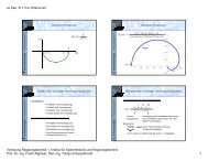
Advanced Solutions <strong>in</strong> Water Networks<br />
Supervisory Pressure Control<br />
• Hydraulic model-based<br />
calculation of optimal set-po<strong>in</strong>t<br />
schedules for pressure<br />
reduction valves (PRVs) for<br />
m<strong>in</strong>imiz<strong>in</strong>g pressure levels <strong>in</strong><br />
District Meter<strong>in</strong>g Areas (DMA)<br />
accord<strong>in</strong>g to predef<strong>in</strong>ed<br />
operational and physical<br />
constra<strong>in</strong>ts<br />
• Used to reduce leakage and<br />
leakage costs as much as<br />
possible <strong>in</strong> DMAs<br />
• Optimal set-po<strong>in</strong>ts can either<br />
be transferred to a local PRVcontroller<br />
or be managed by a<br />
supervisory pressure control<br />
system<br />
•Head [m]<br />
•Time [h]<br />
•Old set-po<strong>in</strong>ts (without optimization)<br />
•New set-po<strong>in</strong>ts (with optimization)<br />
© ABB<br />
| 23
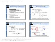
Advanced Solutions <strong>in</strong> Water Networks<br />
Pump and Valve Schedul<strong>in</strong>g<br />
• Hydraulic model-based<br />
generation of optimal set-po<strong>in</strong>t<br />
schedules for pumps, valves<br />
and reservoirs <strong>in</strong> or<strong>der</strong> to<br />
achieve optimal results<br />
follow<strong>in</strong>g the objective function<br />
ma<strong>in</strong>ly to reduce pump<strong>in</strong>g and<br />
water source costs<br />
• Takes <strong>in</strong>to account the<br />
supervisory / global level to<br />
generate optimal schedules<br />
• Uses <strong>in</strong>puts such as demand<br />
forecast<strong>in</strong>g and energy tariffs<br />
<strong>in</strong> or<strong>der</strong> to calculate future<br />
schedules<br />
J = m<strong>in</strong><br />
∑ pump<strong>in</strong>g cost + ∑source<br />
cost +<br />
pumps<br />
sources<br />
∑<br />
demand nodes<br />
leakage cost<br />
© ABB<br />
| 24
Advanced Solutions <strong>in</strong> Water Networks<br />
Model Simplification<br />
• For Supervisory Pressure Control as well as Pump and Valve<br />
Schedul<strong>in</strong>g, a hydraulic optimization model is needed which is <strong>der</strong>ived<br />
from a hydraulic simulation model<br />
• As the simulation model is typically too large and detailed for<br />
optimization purposes <strong>in</strong> terms of number of nodes, pipes, valves and<br />
model accuracy, it is required to reduce the number of objects and to<br />
keep only those needed for the optimization<br />
© ABB<br />
| 25
Advanced Solutions <strong>in</strong> Water Networks<br />
Incident Management – Incident Rank<strong>in</strong>g Table<br />
• In or<strong>der</strong> to enable a more efficient and effective decision mak<strong>in</strong>g, a<br />
model based decision support system provides for an analysis of<br />
possible <strong>in</strong>cidents per identified anomaly<br />
• Based upon assessed impacts and plausibility giv<strong>in</strong>g a risk per<br />
<strong>in</strong>cident, all <strong>in</strong>cidents are ranked accord<strong>in</strong>g to their <strong>in</strong>dividual risk<br />
and thus give guidance to the most important <strong>in</strong>cidents<br />
© ABB<br />
| 26
Advanced Solutions <strong>in</strong> Water Networks<br />
Alarm Management<br />
Berechnung <strong>der</strong> Priorität von<br />
Alarmen<br />
Sortierung <strong>der</strong> Alarme abhängig von<br />
Auswirkung <strong>und</strong><br />
Auftretenswahrsche<strong>in</strong>lichkeit →<br />
Bewertung, welche Alarmmeldung<br />
die höchste Wichtigkeit für den<br />
weiteren Betrieb hat<br />
Negative Auswirkung<br />
für den Betrieb des<br />
Netzes (z.B. Anzahl<br />
<strong>der</strong> kritischen<br />
K<strong>und</strong>en ohne<br />
Wasserversorgung)<br />
Auftretenswahrsche<strong>in</strong>lichkeit<br />
Priorität des Alarms<br />
© ABB Group<br />
June 28, 2010 | Slide 27<br />
© ABB Group<br />
SS 2010 | Slide 27
Advanced Solutions <strong>in</strong> Water Networks<br />
Incident Management – Incident Root Analysis<br />
• The <strong>in</strong>cident root analysis<br />
provides a method for<br />
identify<strong>in</strong>g a pipe <strong>in</strong> cause of<br />
a leakage or burst<br />
• Each potential leakage or<br />
burst location (e.g. pipe<br />
segment) is automatically<br />
assessed with regards to its<br />
likelihood/plausibility of<br />
occurrence and potential<br />
customer impact<br />
© ABB<br />
| 28
Advanced Solutions <strong>in</strong> Water Networks<br />
Incident Management – Incident Impact and Plausibility Viewer<br />
• A decision support system<br />
function graphically <strong>in</strong>dicates<br />
on which pipel<strong>in</strong>e segment the<br />
<strong>in</strong>cident most likely has<br />
occurred<br />
• Representation can be based<br />
upon the assessed impact and<br />
the likelihood of occurrence /<br />
plausibility of a selected<br />
(potential) <strong>in</strong>cident cause that<br />
is taken a closer look at<br />
• The impact reflects the number<br />
of customers that will be<br />
affected by the <strong>in</strong>cident <strong>in</strong> case<br />
of “no action” taken<br />
© ABB<br />
| 29
Advanced Solutions <strong>in</strong> Water Networks<br />
Intervention Management – Network Isolation<br />
• As one of the features,<br />
decision support systems<br />
provide for proposals for<br />
network isolation strategies<br />
• Aims at affect<strong>in</strong>g the least<br />
number of customers when<br />
tak<strong>in</strong>g actions <strong>in</strong> or<strong>der</strong> to<br />
isolate a burst or pipe segment<br />
• Network isolation suggests a<br />
valve or a set of valves to be<br />
closed <strong>in</strong> or<strong>der</strong> to achieve<br />
m<strong>in</strong>imum impact on customer<br />
supplies<br />
© ABB<br />
| 30
Advanced Solutions <strong>in</strong> Water Networks<br />
Intervention Management – Alternative Supplies<br />
• As another feature, decision<br />
support systems provide for<br />
proposals for alternative supply<br />
routes <strong>in</strong> or<strong>der</strong> to ensure<br />
supplies to the maximum<br />
number of customers giv<strong>in</strong>g<br />
valves that need to be<br />
operated <strong>in</strong> or<strong>der</strong> to ensure<br />
supplies<br />
• Alternative supply function<br />
suggests a valve or a set of<br />
valves to be opened <strong>in</strong> or<strong>der</strong> to<br />
achieve best possible supplies<br />
<strong>in</strong> case of required network<br />
isolation<br />
© ABB<br />
| 31
Advanced Solutions <strong>in</strong> Water Networks<br />
Integrated Geographical Information System (GIS)<br />
• GIS Integration <strong>in</strong>to the<br />
automation world<br />
• Make use of mo<strong>der</strong>n objectoriented<br />
approaches<br />
• GIS is used as the ma<strong>in</strong> view to<br />
the process<br />
• A data player (similar to Media<br />
Player) to automatically visualize<br />
future network status (us<strong>in</strong>g<br />
results from network simulation)<br />
© ABB<br />
| 32
Decision Support System for<br />
Burst Localisation
Burst Localisation<br />
Failures <strong>in</strong> Water Distribution Systems<br />
• True cause typically unknown<br />
• Identification of failure by comb<strong>in</strong><strong>in</strong>g evidence<br />
• Measurements<br />
• Alarms & Events<br />
• Customer compla<strong>in</strong>ts<br />
• Pipe bursts<br />
• Most relevant problem<br />
• Provide relevant<br />
<strong>in</strong>formation to the<br />
operator
Burst Localisation<br />
Risk-based approach<br />
• Evaluation of risk associated with failures<br />
• Risk components:<br />
• Likelihood (of a failure)<br />
• Impact (of a failure)<br />
• Risks should be known from the beg<strong>in</strong>n<strong>in</strong>g<br />
• Risk changes with time!<br />
• Used to prioritise failures
Burst Localisation<br />
Likelihood Estimation<br />
Comb<strong>in</strong>ed Evidence<br />
Credibility<br />
adjusted based on<br />
performance…<br />
weights<br />
•<br />
w 1 w 2 w 3 w 4 w N<br />
Burst Prediction<br />
Model<br />
Correlated Customer<br />
Contacts<br />
Identification Us<strong>in</strong>g<br />
Hydraulic Model<br />
Operator’s<br />
Judgement<br />
...<br />
Field Technician’s<br />
Evidence<br />
• Information fusion us<strong>in</strong>g Dempster-Shafer Theory* of Evidence<br />
• Could be hierarchical<br />
It allows one to comb<strong>in</strong>e evidence from different sources and arrive at a degree of belief<br />
(represented by a belief function) that takes <strong>in</strong>to account all the available evidence. The theory<br />
was first developed by Arthur P. Dempster and Glenn Shafer.<br />
(http://en.wikipedia.org/wiki/Dempster-Shafer_theory)
Burst Localisation<br />
Pipe burst prediction model<br />
• Type of soil<br />
• Land use<br />
• Age of pipe<br />
• Material type<br />
• Diameter<br />
• Number of days of air frost<br />
• Monthly mean m<strong>in</strong>imum temperature<br />
f( S, LAM , , , DA , , T )<br />
F<br />
m<strong>in</strong>
Burst Localisation<br />
Customer Contacts Model<br />
• Relates likelihood of pipe failure to<br />
the distance from a group of<br />
customers<br />
• Only post code is known<br />
• Evaluated us<strong>in</strong>g GIS<br />
• If sufficient many compla<strong>in</strong>ts from<br />
a certa<strong>in</strong> area arrive, there is a<br />
good <strong>in</strong>dication for a problem <strong>in</strong><br />
that area.<br />
Customer 1 Customer 2<br />
<br />
Customer 4<br />
Customer 3
Burst Localisation<br />
Information Process<strong>in</strong>g<br />
Criterion Measurement<br />
Model<br />
Static Evidence<br />
Dynamic Evidence<br />
Asset data GIS Device Customer Near real-time<br />
Status Contacts pressure and flow<br />
data
Burst Localisation<br />
Case Study 1<br />
• Rural DMA *<br />
• Tree network<br />
• 181 residential and 57<br />
<strong>in</strong>dustrial customers<br />
• 3 pressure sensors and 1 flow<br />
meter<br />
*DMA – District Meter<strong>in</strong>g Area<br />
•40
•41
•42
•43
•44
Burst Localisation<br />
Case Study 2<br />
• Urban DMA<br />
• Looped network<br />
• 3900 customers<br />
• 3 pressure sensors and 2<br />
flow meters<br />
•45
Pipe burst prediction<br />
•46
Hydraulic model<br />
•47
Customer contact<br />
•48
•49
Water Network Modell<strong>in</strong>g<br />
Network Simplification<br />
© ABB Group<br />
June 28, 2010 | Slide 50
Network Simplification<br />
Why use simplification?<br />
• Produce hydraulically equivalent water networks with<br />
reduced number of pipes and nodes only conta<strong>in</strong><strong>in</strong>g<br />
• critical nodes (nodes with pressure constra<strong>in</strong>ts)<br />
• active elements (e.g. pumps, valves, reservoirs, tanks)<br />
• Use reduced water networks as base for follow<strong>in</strong>g<br />
simulation and optimization<br />
• Reduce calculation time by reduc<strong>in</strong>g number of<br />
equations and constra<strong>in</strong>ts<br />
© ABB Group<br />
June 28, 2010 | Slide 51
Network Simplification<br />
Steps of the simplification algorithm<br />
• The algorithms consists of two parts<br />
• Pre-process<strong>in</strong>g<br />
• Substitute valves that are always open<br />
• Remove valves that are always closed<br />
• Remove dead-end pipes<br />
• Remove short pipes<br />
• Comb<strong>in</strong>e pipes <strong>in</strong> series / <strong>in</strong> parallel connected to nodes<br />
without demand to <strong>uni</strong>que pipe<br />
• Gauss-Jordan Simplification<br />
• Determ<strong>in</strong>e nonl<strong>in</strong>ear model<br />
• L<strong>in</strong>earize nonl<strong>in</strong>ear model<br />
• Reduce l<strong>in</strong>earized model us<strong>in</strong>g Gauss-Jordan<br />
• Convert back to nonl<strong>in</strong>ear model<br />
© ABB Group<br />
June 28, 2010 | Slide 52
Preprocess<strong>in</strong>g<br />
Substitute valves that are always open<br />
• A permanently opened valve can be removed<br />
•reservoir<br />
•reservoir<br />
•Opened<br />
•valve<br />
•closed<br />
•closed<br />
•valve<br />
•tank<br />
•valve<br />
•tank<br />
© ABB Group<br />
June 28, 2010 | Slide 53
Preprocess<strong>in</strong>g<br />
Remove valves that are always closed<br />
• The closed valve is removed<br />
•reservoir<br />
•reservoir<br />
•closed<br />
•valve<br />
•tank<br />
•tank<br />
© ABB Group<br />
June 28, 2010 | Slide 54
Preprocess<strong>in</strong>g<br />
Remove dead-end pipes<br />
• Junctions without demands at the end of pipe l<strong>in</strong>es can be<br />
removed as they cause numerical problems and do not<br />
have any function <strong>in</strong> the model<br />
•reservoir<br />
•reservoir<br />
•tank<br />
•tank<br />
© ABB Group<br />
June 28, 2010 | Slide 55
Preprocess<strong>in</strong>g<br />
Remove short pipes<br />
• Short pipes have high conductance / low resistance,<br />
therefore the headloss nearly vanishes and can be<br />
removed from the model<br />
•reservoir<br />
•reservoir<br />
•tank<br />
•tank<br />
© ABB Group<br />
June 28, 2010 | Slide 56
Preprocess<strong>in</strong>g<br />
Comb<strong>in</strong>e pipes <strong>in</strong> series with demandless nodes /<br />
<strong>in</strong> parallel to <strong>uni</strong>que pipe<br />
• Pipes <strong>in</strong> series with junctions, which have no demand, has the<br />
same hydraulic effect as one pipe with an equivalent<br />
conductance/resistance value and thus can be substituted<br />
(R=R1+R2)<br />
• Parallel pipe can be substituted with a <strong>uni</strong>que pipe, which has the<br />
aggregate conductance of the orig<strong>in</strong>al ones (1/R = 1/R1 + 1/R2)<br />
•reservoir<br />
•reservoir<br />
© ABB Group<br />
June 28, 2010 | Slide 57<br />
•Node with demand<br />
•tank<br />
•tank
Gauss-Jordan Simplification<br />
Full nonl<strong>in</strong>ear<br />
model<br />
Use po<strong>in</strong>t <strong>in</strong> time with max. number<br />
of pipes with flow > 0 to l<strong>in</strong>earize<br />
network<br />
L<strong>in</strong>earize model<br />
Full l<strong>in</strong>ear<br />
model<br />
Use Gauss-Jordan algorithm to<br />
reduce number of nodes and pipes<br />
Simplify model<br />
Simplified<br />
l<strong>in</strong>ear model<br />
Convert back to<br />
nonl<strong>in</strong>ear model<br />
© ABB Group<br />
June 28, 2010 | Slide 58<br />
Calculate new nonl<strong>in</strong>ear pipe<br />
parameters us<strong>in</strong>g <strong>in</strong>cidence matrix<br />
(C=100, D=L)<br />
Simplified<br />
nonl<strong>in</strong>ear model
Gauss-Jordan Simplification<br />
Determ<strong>in</strong>e nonl<strong>in</strong>ear model<br />
reservoir<br />
demand<br />
demand<br />
• Setup <strong>in</strong>cidence matrix to describe model of water network<br />
tank<br />
demand<br />
demand<br />
⎡ 1<br />
⎢<br />
⎢<br />
−1<br />
⎢ 0<br />
Λ = ⎢<br />
⎢ 0<br />
⎢ 0<br />
⎢<br />
⎣ 0<br />
|<br />
0<br />
1<br />
−1<br />
0<br />
0<br />
0<br />
0<br />
0<br />
1<br />
−1<br />
0<br />
0<br />
h |<br />
0.54<br />
0<br />
0<br />
1<br />
0<br />
−1<br />
0<br />
0<br />
0<br />
0<br />
1<br />
−1<br />
0<br />
sign(<br />
∆<br />
0 ⎤<br />
0<br />
⎥<br />
⎥<br />
0 ⎥<br />
⎥<br />
1 ⎥<br />
0 ⎥<br />
⎥<br />
−1<br />
⎦<br />
The Hazen-Williams equation describes<br />
the flow-head relationship <strong>in</strong> a pipe<br />
Q<br />
ij<br />
=<br />
g<br />
ij<br />
∆<br />
ij<br />
ij<br />
h)<br />
Λq = q<br />
nod<br />
Mass balance equation<br />
∆h<br />
T<br />
= Λ<br />
h<br />
Headloss equation<br />
© ABB Group<br />
June 28, 2010 | Slide 59
Gauss-Jordan Simplification<br />
L<strong>in</strong>earization of model<br />
• Start<strong>in</strong>g po<strong>in</strong>t for subsequent l<strong>in</strong>earization is<br />
Λ )<br />
T<br />
Q ( Λ h =<br />
q<br />
nod<br />
• After l<strong>in</strong>earization we get<br />
dQ<br />
Λ Λ<br />
d∆h<br />
T<br />
nod nod<br />
⋅ ( h − h(<br />
t0 )) = ( q − q ( t0<br />
))<br />
•<br />
• Us<strong>in</strong>g<br />
Q<br />
ij<br />
=<br />
g<br />
ij<br />
|<br />
∆<br />
ij<br />
h<br />
|<br />
0.54<br />
sign(<br />
∆<br />
ij<br />
h)<br />
© ABB Group<br />
June 28, 2010 | Slide 60<br />
• we obta<strong>in</strong><br />
dQ<br />
=<br />
d∆h<br />
diag<br />
−0.46<br />
[ 0.54g ] J j<br />
| ∆h j<br />
|<br />
j<br />
= 1
Gauss-Jordan Simplification<br />
Setup of l<strong>in</strong>earized equations system<br />
• Def<strong>in</strong><strong>in</strong>g Matrix A as<br />
dQ<br />
A = Λ Λ<br />
d∆h<br />
• We obta<strong>in</strong> for each element<br />
A<br />
[ n,<br />
m]<br />
∑<br />
T<br />
⎧−<br />
Anm<br />
for n = m<br />
⎪ m≠n<br />
⎪<br />
−<br />
= ⎨<br />
− 0.54gn,<br />
m<br />
| hn<br />
− hm<br />
|<br />
⎪<br />
⎪<br />
⎩ 0 for n ≠ m and<br />
0.46<br />
= : −g~<br />
( n,<br />
m)<br />
nm<br />
for n ≠ m and<br />
( n,<br />
m)<br />
connected by a<br />
not connected by a l<strong>in</strong>k<br />
l<strong>in</strong>k<br />
• and can therefore build the follow<strong>in</strong>g equations system<br />
nod<br />
⎛ g~<br />
− g~<br />
− g~<br />
11<br />
1,2<br />
...<br />
1, N ⎞⎛<br />
δh1<br />
⎞ ⎛δq<br />
⎞<br />
1<br />
⎜<br />
⎟⎜<br />
⎟ ⎜ ⎟<br />
nod<br />
⎜ − g~<br />
g~<br />
− g~<br />
2,1 22<br />
...<br />
2, N ⎟⎜<br />
δh2<br />
⎟ ⎜δq2<br />
⎟<br />
⎜<br />
⎟⎜<br />
⎟ =<br />
... ... ... ... ...<br />
⎜ ⎟<br />
⎜<br />
⎟⎜<br />
⎟ ⎜<br />
...<br />
⎟<br />
nod<br />
⎝−<br />
g~<br />
N<br />
− g~<br />
N<br />
... g~<br />
,1<br />
,2<br />
NN ⎠⎝δhN<br />
⎠ ⎝δq<br />
N ⎠<br />
© ABB Group<br />
June 28, 2010 | Slide 61
© ABB Group<br />
June 28, 2010 | Slide 62<br />
Gauss-Jordan Simplification<br />
Elim<strong>in</strong>ation of nodes<br />
• Elim<strong>in</strong>at<strong>in</strong>g node 1 from the equations system leads to a reduced<br />
equation system<br />
⎟<br />
⎟<br />
⎟<br />
⎟<br />
⎟<br />
⎠<br />
⎞<br />
⎜<br />
⎜<br />
⎜<br />
⎜<br />
⎜<br />
⎝<br />
⎛<br />
=<br />
⎟<br />
⎟<br />
⎟<br />
⎟<br />
⎟<br />
⎠<br />
⎞<br />
⎜<br />
⎜<br />
⎜<br />
⎜<br />
⎜<br />
⎝<br />
⎛<br />
⎟<br />
⎟<br />
⎟<br />
⎟<br />
⎟<br />
⎠<br />
⎞<br />
⎜<br />
⎜<br />
⎜<br />
⎜<br />
⎜<br />
⎝<br />
⎛<br />
−<br />
−<br />
−<br />
−<br />
−<br />
−<br />
nod<br />
N<br />
nod<br />
nod<br />
N<br />
NN<br />
N<br />
N<br />
N<br />
N<br />
q<br />
q<br />
q<br />
h<br />
h<br />
h<br />
g<br />
g<br />
g<br />
g<br />
g<br />
g<br />
g<br />
g<br />
g<br />
δ<br />
δ<br />
δ<br />
δ<br />
δ<br />
δ<br />
...<br />
...<br />
~<br />
...<br />
~<br />
~<br />
...<br />
...<br />
...<br />
...<br />
~<br />
...<br />
~<br />
~<br />
~<br />
...<br />
~<br />
~<br />
2<br />
1<br />
2<br />
1<br />
,2<br />
,1<br />
2,<br />
22<br />
2,1<br />
1,<br />
1,2<br />
11<br />
⎟<br />
⎟<br />
⎟<br />
⎟<br />
⎟<br />
⎟<br />
⎠<br />
⎞<br />
⎜<br />
⎜<br />
⎜<br />
⎜<br />
⎜<br />
⎜<br />
⎝<br />
⎛<br />
+<br />
+<br />
=<br />
⎟<br />
⎟<br />
⎟<br />
⎠<br />
⎞<br />
⎜<br />
⎜<br />
⎜<br />
⎝<br />
⎛<br />
⎟<br />
⎟<br />
⎟<br />
⎟<br />
⎟<br />
⎟<br />
⎠<br />
⎞<br />
⎜<br />
⎜<br />
⎜<br />
⎜<br />
⎜<br />
⎜<br />
⎝<br />
⎛<br />
⎟<br />
⎟<br />
⎠<br />
⎞<br />
⎜<br />
⎜<br />
⎝<br />
⎛<br />
−<br />
⎟<br />
⎟<br />
⎠<br />
⎞<br />
⎜<br />
⎜<br />
⎝<br />
⎛<br />
−<br />
−<br />
⎟<br />
⎟<br />
⎠<br />
⎞<br />
⎜<br />
⎜<br />
⎝<br />
⎛<br />
−<br />
−<br />
⎟<br />
⎟<br />
⎠<br />
⎞<br />
⎜<br />
⎜<br />
⎝<br />
⎛<br />
−<br />
nod<br />
N<br />
nod<br />
N<br />
nod<br />
nod<br />
N<br />
N<br />
N<br />
N<br />
N<br />
N<br />
N<br />
N<br />
q<br />
g<br />
g<br />
q<br />
q<br />
g<br />
g<br />
q<br />
h<br />
h<br />
g<br />
g<br />
g<br />
g<br />
g<br />
g<br />
g<br />
g<br />
g<br />
g<br />
g<br />
g<br />
g<br />
g<br />
g<br />
g<br />
1<br />
1<br />
,1<br />
1<br />
1<br />
2,1<br />
2<br />
2<br />
1,<br />
11<br />
,1<br />
1,2<br />
11<br />
,1<br />
,2<br />
1,<br />
11<br />
2,1<br />
2,<br />
1,2<br />
11<br />
2,1<br />
22<br />
~<br />
~<br />
...<br />
~<br />
~<br />
...<br />
~<br />
~<br />
~<br />
~<br />
...<br />
~<br />
~<br />
~<br />
~<br />
...<br />
...<br />
...<br />
~<br />
~<br />
~<br />
~<br />
...<br />
~<br />
~<br />
~<br />
~<br />
δ<br />
δ<br />
δ<br />
δ<br />
δ<br />
δ
Gauss-Jordan Simplification<br />
Setup of l<strong>in</strong>earized equations system<br />
• Once all nodes selected have been elim<strong>in</strong>ated, the equation system<br />
can be reconverted to a nonl<strong>in</strong>ear one us<strong>in</strong>g follow<strong>in</strong>g assumptions<br />
• R n,m = 100 (Roughness)<br />
• D=L (D)iameter and (L)ength of pipe<br />
⎛ ⎛<br />
⎜<br />
⎜<br />
⎜ g~<br />
⎝<br />
⎜<br />
⎜⎛<br />
⎜<br />
⎜<br />
⎜−<br />
g~<br />
⎝⎝<br />
22<br />
N ,2<br />
g~<br />
2,1<br />
− g~<br />
g~<br />
1,2<br />
11<br />
...<br />
g~<br />
N ,1<br />
− g~<br />
g~<br />
11<br />
⎞<br />
⎟<br />
⎠<br />
1,2<br />
⎞<br />
⎟<br />
⎠<br />
...<br />
...<br />
...<br />
⎛<br />
⎜−<br />
g~<br />
⎝<br />
⎛<br />
⎜ g~<br />
⎝<br />
2, N<br />
0.54g g~<br />
−0.46<br />
n, m<br />
| hn<br />
− hm<br />
| =<br />
N<br />
g~<br />
−<br />
g~<br />
...<br />
g~<br />
−<br />
g~<br />
N ,1<br />
11<br />
2,1<br />
11<br />
g~<br />
nm<br />
g~<br />
1, N<br />
1, N<br />
⎞⎞<br />
⎟<br />
⎟<br />
⎟⎛<br />
δh<br />
⎠ ⎜<br />
⎟<br />
⎜ ...<br />
⎞ ⎟<br />
⎜<br />
⎟<br />
⎟ ⎝δh<br />
⎠ ⎟<br />
⎠<br />
2<br />
N<br />
⎛<br />
⎜ δq<br />
⎞<br />
⎟ ⎜<br />
⎟ = ⎜<br />
⎟ ⎜<br />
⎠<br />
⎜δq<br />
⎝<br />
nod<br />
2<br />
nod<br />
N<br />
+<br />
+<br />
g~<br />
g~<br />
...<br />
g~<br />
g~<br />
2,1<br />
1<br />
N ,1<br />
1<br />
δq<br />
δq<br />
nod<br />
1<br />
nod<br />
1<br />
⎞<br />
⎟<br />
⎟<br />
⎟<br />
⎟<br />
⎟<br />
⎠<br />
D<br />
n,<br />
m<br />
⎛ g<br />
⎜<br />
⎝ 3.58821⋅10<br />
n,<br />
m<br />
= Ln,<br />
m<br />
=<br />
−4<br />
⎞<br />
⎟<br />
⎠<br />
1<br />
2.09<br />
© ABB Group<br />
June 28, 2010 | Slide 63
Gauss-Jordan Simplification<br />
Simplified water network<br />
•pre-processed model<br />
reservoir<br />
•simplified model<br />
reservoir<br />
demand<br />
demand<br />
demand<br />
demand<br />
demand<br />
demand<br />
tank<br />
tank<br />
© ABB Group<br />
June 28, 2010 | Slide 64
Example of Water Distribution Network (E093.<strong>in</strong>p)<br />
•Reservoir<br />
•Nodes to keep<br />
•Nodes with high<br />
elevation or<br />
demand<br />
•„normal“ nodes<br />
© ABB Group<br />
June 28, 2010 | Slide 65
Simplified network<br />
© ABB Group<br />
June 28, 2010 | Slide 66
Simplified network<br />
Comparison<br />
• All active elements like pumps, reservoirs, tanks and<br />
valves (except they do not change their status dur<strong>in</strong>g the<br />
complete simulation time) are kept<br />
Before simplification<br />
After simplification<br />
© ABB Group<br />
June 28, 2010 | Slide 67
Compare orig<strong>in</strong>al and simplified network<br />
Compare pressures<br />
the accuracy is sufficient!<br />
© ABB Group<br />
June 28, 2010 | Slide 68
Example: network with 12527 nodes<br />
© ABB Group<br />
June 28, 2010 | Slide 69
Example: network with 12527 nodes<br />
Simplified by 50%<br />
© ABB Group<br />
June 28, 2010 | Slide 70
Water Network Optimization<br />
Pumpen- <strong>und</strong> Ventile<strong>in</strong>satzplanung<br />
© ABB Group<br />
June 28, 2010 | Slide 71
Pump & Valve schedul<strong>in</strong>g<br />
Challenges <strong>in</strong> Network Operation<br />
• Generate optimized pump, valve and water source trajectories to<br />
m<strong>in</strong>imize energy costs, source costs and leakage <strong>in</strong> WDN*<br />
• look 24 hours ahead to know what the water demand, the<br />
electricity tariffs and the treatment costs will be<br />
• use full range of possible water levels <strong>in</strong> reservoirs to fill<br />
reservoirs when it fits best to optimization strategy<br />
• withdraw water from water sources <strong>in</strong> an cost-optimal way,<br />
tak<strong>in</strong>g <strong>in</strong>to account operational constra<strong>in</strong>ts<br />
• operate pumps tak<strong>in</strong>g <strong>in</strong>to account actual and future electricity<br />
costs, consi<strong>der</strong><strong>in</strong>g pump efficiencies to choose optimal pump<br />
speed<br />
• BUT: always keep with<strong>in</strong> physical and operational constra<strong>in</strong>ts,<br />
such as ma<strong>in</strong>ta<strong>in</strong><strong>in</strong>g sufficient water with<strong>in</strong> the system’s<br />
reservoirs or meet<strong>in</strong>g the required time-vary<strong>in</strong>g consumer<br />
demands<br />
© ABB Group<br />
June 28, 2010 | Slide 72<br />
*Water Distribution Network
Pump & Valve schedul<strong>in</strong>g<br />
Optimization Problem<br />
J<br />
= m<strong>in</strong><br />
∑ pump<strong>in</strong>g cost + ∑source<br />
cost +<br />
pumps<br />
sources<br />
∑<br />
demand nodes<br />
leakage<br />
cost<br />
• Gegeben ist die reduzierte Modellbeschreibung des<br />
Wassernetzes.<br />
• Gegeben s<strong>in</strong>d physikalische <strong>und</strong> betriebliche<br />
Beschränkungen <strong>der</strong> Mess- <strong>und</strong> Stellvariablen<br />
(Durchflüsse, Drücke, Pumpleistungen,<br />
Reservoirgrößen etc.)<br />
• Gegeben ist e<strong>in</strong>e Vorhersage des Verbrauches <strong>und</strong><br />
<strong>der</strong> Stromkosten <strong>der</strong> nächsten 24 St<strong>und</strong>en<br />
F<strong>in</strong>de e<strong>in</strong>e optimale Steuerstrategie, die J<br />
m<strong>in</strong>imiert, die Beschränkungen e<strong>in</strong>hält <strong>und</strong> dem<br />
Modell entspricht.<br />
© ABB Group<br />
June 28, 2010 | Slide 73
Example of a Water Network Schematic<br />
• 3537 Nodes (non<br />
simplified)<br />
• 3 Water Treatment<br />
Works (WTW)<br />
• 10 Reservoirs<br />
• 11 Pump<strong>in</strong>g Stations<br />
(19 pumps)<br />
• 80 DMA<br />
• 420 valves<br />
• 3 <strong>in</strong>dustrial users<br />
• 5.2m kWh (2008)<br />
© ABB Group<br />
June 28, 2010 | Slide 74<br />
conta<strong>in</strong>s several<br />
s<strong>in</strong>gle and<br />
cascad<strong>in</strong>g DMAs<br />
with 500 – 1000<br />
nodes each
Pump & Valve schedul<strong>in</strong>g<br />
Current operation vs. Optimal schedule<br />
© ABB Group<br />
June 28, 2010 | Slide 75
Pump & Valve schedul<strong>in</strong>g<br />
Results from the case study<br />
© ABB Group<br />
June 28, 2010 | Slide 76<br />
• 7 days optimization<br />
• Only Pump and valve schedul<strong>in</strong>g, no WTW *<br />
schedul<strong>in</strong>g<br />
• Reservoir level limits (40%-95%)<br />
• Fixed WTW outflows<br />
• Initial start<strong>in</strong>g values for reservoir levels:<br />
(M<strong>in</strong>+Max)/2<br />
For 7 days<br />
Pump<strong>in</strong>g Energy [kW/h] Pump<strong>in</strong>g Costs [£]<br />
Current<br />
Operation<br />
Optimized<br />
Operation<br />
Current<br />
Operation<br />
Optimized<br />
Operation<br />
Total 51902 35901 3817 2483<br />
Sav<strong>in</strong>gs 16001 1334<br />
Sav<strong>in</strong>gs [%] 30.8 34.9<br />
*Water Treatment Work
Anwendung Wassernetz Basel<br />
Problembeschreibung<br />
• Industrielle Werke Basel (IWB) – bâlAqua<br />
• 12 high pressure pumps<br />
• One <strong>in</strong>ternal gro<strong>und</strong> water dra<strong>in</strong>age and collection area,<br />
<strong>in</strong>clud<strong>in</strong>g 12 wells (with low pressure pumps)<br />
• One external supplier<br />
• Three double chamber reservoirs<br />
• Roughly 26 million m 3 of annual delivery<br />
• F<strong>in</strong>d an energy-optimal pump (and wells) schedule to<br />
provide sufficient amount of water (based on predictions)<br />
with m<strong>in</strong>imal pump<strong>in</strong>g effort.<br />
© ABB Group<br />
SS 2010 | Slide 77
Anwendung Wassernetz Basel<br />
Problem Formulierung<br />
• Optimally solve a hybrid problem consist<strong>in</strong>g of<br />
• ... cont<strong>in</strong>uous variables (eg, flows, levels, energy etc.)<br />
and<br />
• ... discrete variables (as for example switch<strong>in</strong>g the plant<br />
equipment on/off).<br />
• Such a problem can be formulated us<strong>in</strong>g Mixed-Logical<br />
Dynamic Models (MLD) and subsequently be solved used<br />
an MPC controller.<br />
• Possible implementation strategies<br />
• Optimization – Solve problem complete <strong>in</strong> advance<br />
• Control – Update solution onl<strong>in</strong>e <strong>in</strong> each time step<br />
© ABB Group<br />
SS 2010 | Slide 78
Anwendung Wassernetz Basel<br />
Implementierung<br />
Benefits<br />
• Information <strong>in</strong>tegration<br />
• Cost optimization<br />
© ABB Group<br />
SS 2010 | Slide 79
Zusammenfassung<br />
• Wasser – e<strong>in</strong> Megatrend des 21. Jahrh<strong>und</strong>erts<br />
• Wichtigste Automatisierungsgebiete r<strong>und</strong> um Wasser<br />
• Tr<strong>in</strong>kwasserversorgungsnetze (Operation, Plann<strong>in</strong>g, Monitor<strong>in</strong>g)<br />
• Meerwasserentsalzung (Monitor<strong>in</strong>g, Optimization)<br />
• Abwasserentsorgung (Instrumentation, Operation)<br />
• Bewässerung <strong>in</strong> <strong>der</strong> Landwirtschaft (Optimization)<br />
• Wasserwirtschaft <strong>in</strong> <strong>der</strong> Industrie (Instrumenation, Optimization)<br />
• Informations<strong>in</strong>tegration ist die größte Herausfor<strong>der</strong>ung <strong>in</strong><br />
e<strong>in</strong>em gewachsenen, verteilten System das sehr alt ist.<br />
• Darauf aufbauend s<strong>in</strong>d mo<strong>der</strong>ne Verfahren verfügbar, die<br />
signifikante E<strong>in</strong>sparungen <strong>und</strong> Verbesserungen<br />
ermöglichen.<br />
• Wasser<strong>in</strong>dustrie gilt als beson<strong>der</strong>s konservativ.<br />
• Unterschiedliche Modellbeschreibungen s<strong>in</strong>d <strong>der</strong> Schlüssel<br />
für gehobene Lösungen.<br />
© ABB Group<br />
SS 2010 | Slide 80
Referenzen<br />
• http://www.zvei.org/fileadm<strong>in</strong>/user_upload/Fachverbaende/Automation/Publikation/Bestell<br />
formular_Roadmap_Wasser_<strong>und</strong>_Abwasser.pdf<br />
• D.Moll, T.v.Hoff, M.Anto<strong>in</strong>e, Tapp<strong>in</strong>g Technology - Optimiz<strong>in</strong>g the water supply for the<br />
city of Basel. ABB Review 3/2007, pp. 27-30.<br />
• Gallestey, E, et al., Us<strong>in</strong>g Model Predictive Control and Hybrid Systems for Optimal<br />
Schedul<strong>in</strong>g of Industrial Processes, Automatisierungstechnik, Vol. 51, No. 6, 2003.<br />
• Public (EPSRC <strong>in</strong> UK) f<strong>und</strong>ed Research & Development project ‚NEPTUNE‘.<br />
(http://www.neptune.ac.uk)<br />
• Bogumil Ulanicki, Hossam AbdelMeguid, Peter Bo<strong>und</strong>s and Ridwan Patel (2008),<br />
PRESSURE CONTROL IN DISTRICT METERING AREAS WITH BOUNDARY AND<br />
INTERNAL PRESSURE REDUCING VALVES, Proceed<strong>in</strong>gs of the 10th Annual Water<br />
Distribution Systems Analysis Conference WDSA2008, Van Zyl, J.E., Ilemobade, A.A.,<br />
Jacobs, H.E. (eds.), August 17-20, 2008, Kruger National Park, South Africa.<br />
• B.Ulanicki, A.Zehnpf<strong>und</strong> and F.Mart<strong>in</strong>ez (1996), Simplification of Water Distribution<br />
Network Models. In Proceed<strong>in</strong>gs of the Hydro<strong>in</strong>formatics 96 Int. Conf. International<br />
Assoc. for Hydraulic Research, ETH Zürich, Sep 1996.<br />
© ABB Group<br />
SS 2010 | Slide 81
Kontakt<br />
Dr. Alexan<strong>der</strong> Horch<br />
ABB Forschungszentrum<br />
Wallstadter Straße 59<br />
68526, Ladenburg, GERMANY<br />
L<strong>in</strong>ks<br />
www.abb.de/forschung<br />
www.abb.de/karriere<br />
Phone: +49 6203716021<br />
Telefax: +49 6203 716253<br />
Mobile: +49 171 307 6403<br />
Email: alexan<strong>der</strong>.horch@de.abb.com<br />
© ABB Group<br />
SS 2010 | Slide 82